EDBT Summer School

Database Performance

Pat & Betty (Elizabeth) O’Neil

Sept. 6, 2007

2

Database Performance: Outline Here is an outline of our two-lecture course

First, we explain why OLTP performance is no longer thought tobe an important problem by most researchers and developers

But we’ll introduce a new popular Transactional product calledSnapshot Isolation that supports updates & concurrent queries

Then we look at queries, especially Data Warehouse queries,which get the most performance attention currently

We explain early query performance concepts, e.g. index FilterFactor, then look at cubical clustering, the new crucial factor

Data Warehousing is where most new purchases are made atpresent, and we examine the area in detail

3

DB Performance: OLTP Jim Gray said years ago: OLTP is a solved problem

Older established companies that do OLTP Order Entry havesolutions in place, efficient enough not to need change

One reason is that change is very difficult: rewriting a company’sOLTP programs is called the “Dusty Decks” problem

Nobody remembers how all the code works!

Also, the cost of hardware to support update transactionscompared to programming costs, or even terminal costs, is low

We explain this in the slides immediately following

But some new installations use new transactional approachesthat better support queries, such as Snapshot Isolation

We explain Snapshot Isolation a bit later (starting on Slide 7)

4

OLTP DebitCredit Benchmark

Anon [Jim Gray] et al. paper (in Datamation, 1985)introduced the DebitCredit benchmark.

Bank Transaction tables: Acct, Teller, Brnch, History, with 100 byte rows

Read 100 bytes from terminal: aid, tid, bid, delta Begin Transaction;

Update Accnt set Accnt_bal = Accnt_bal +:delta where Accnt_ID = :aid;Insert to History values (:aid,:tid, :bid, :delta, Time_stamp);Update Teller set Teller_bal = Teller_bal + :delta where Teller_ID = :tid;Update Brnch set Brnch_bal = Brnch_bal+:delta where Brnch_ID = :bid;

Commit;Write 200 bytes to terminal including: aid, tid, bid, delta, Accnt_bal

Transactions per second (tps) scaled with size of tables: each tps had100,000 Accnts, 10 Brnches, 100 Tellers; History held 90 days of inserts1History of DebitCredit/TPC-A in Jim Gray’s “The Benchmark Handbook”, Chapter 2.

5

OLTP DebitCredit Benchmark DebitCredit restrictions; performance features tested

Terminal request response time required 95% under 1 second;throughput driver had to be titrated to give needed response

Think time was 100 secs (after response): meant much contexthad to be held in memory for terminals (10,000 for 100 tps)

Terminal simulators were used; Variant TP1 benchmark drovetransactions by software loop generation with trivial think time

Mirrored Tx logs required to provide guaranteed recovery

History Inserts (50 byte rows) costly if pages locked

System had to be priced, measured in $/tps

6

OLTP DebitCredit/TPC-A Benchmark Vendors cheated when running DebitCredit Jim Gray welcomed new Transaction Processing Performance

Council (TPC), consortium of vendors, created TPC-A1 in 1989 Change from DebitCredit: measurement rules were carefully

specified and auditors were required for results to be published Detail changes:

For each 1 tps, only one Branch instead of 10: meant concurrencywould be tougher: important to update Branch LAST

Instead of 100 sec Think Time, used 10 sec. Unrealistic, but reasonwas that TERMINAL PRICES WERE TOO HIGH WITH 100 SEC!Terminal prices were more than all other costs for benchmark Even in 1989, transactions were cheap to run!

1History of DebitCredit/TPC-A in Jim Gray’s “The Benchmark Handbook”, Chapter 2. In ACMSIGMOD Anthology, http://www.sigmod.org/dblp/db/books/collections/gray93.html

7

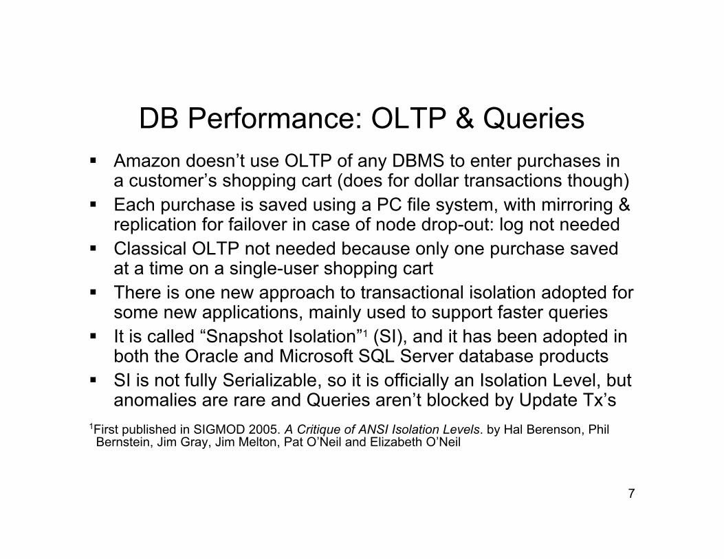
DB Performance: OLTP & Queries Amazon doesn’t use OLTP of any DBMS to enter purchases in

a customer’s shopping cart (does for dollar transactions though) Each purchase is saved using a PC file system, with mirroring &

replication for failover in case of node drop-out: log not needed Classical OLTP not needed because only one purchase saved

at a time on a single-user shopping cart There is one new approach to transactional isolation adopted for

some new applications, mainly used to support faster queries It is called “Snapshot Isolation”1 (SI), and it has been adopted in

both the Oracle and Microsoft SQL Server database products SI is not fully Serializable, so it is officially an Isolation Level, but

anomalies are rare and Queries aren’t blocked by Update Tx’s1First published in SIGMOD 2005. A Critique of ANSI Isolation Levels. by Hal Berenson, Phil Bernstein, Jim Gray, Jim Melton, Pat O’Neil and Elizabeth O’Neil

8

DB Performance: Snapshot Isolation (SI) A transaction Ti executing under Snapshot Isolation (SI) reads

only committed data as of the time Start(Ti ) This doesn’t work by taking a “snapshot” of all data when new

Tx starts, but by taking a timestamp and keeping old versions ofdata when new versions are written: Histories in SI read & write“versions” of data items

Data read, including both row values and indexes, time travelsto Start(Ti), so predicates read by Ti also time travel to Start(Ti)

A transaction Ti in SI also maintains data it has written in a localcache, so if it rereads this data, it will read what it wrote

No Tk concurrent with Ti (overlapping lifetimes) can read what Tihas written (can only read data committed as of Start(Tk))

If concurrent transactions both update same data item A, thensecond one trying to commit will abort (First committer wins rule)

9

DB Performance: Snapshot Isolation (SI) SI Histories read and write Versions of data items: (X0, X1, X2);

X0 is value before updates, X2 would be written by T2, X7 by T7 Standard Tx’l anomalies of non-SR behavior don’t occur in SI Lost Update anomaly in Isolation Level READ COMMITTED

(READ COMMITTED is Default Isolation Level on all DB products) : (I’m underlining T2’s operations just to group them visually)

H1: R1(X,50) R2(X,50) W2(X,70) C2 W1(X,60) C1 (X should be 80)

In SI, First Committer Wins property prevents this anomaly:H1SI: R1(X0,50) R2(X0,50) W2(X2,70) C2 W1(X1,60) A1

Inconsistent View anomaly possible in READ COMMITTED:H2: R1(X,50) R2(X,50) W2(X,70) R2(Y,50) W2(Y,30) C2 R1(Y,30) C1

Here T1 sees X+Y = 80; In SI, Snapshot Read avoids this anomalyH2SI: R1(X0,50) R2(X0,50) W2(X2,70) R2(Y0,50) W2(Y2,30) C2R1(Y0,50) C1 (T1 reads sum of X+Y = 100, valid at Start(T1)

10

DB Performance: Snapshot Isolation

In SI, READ-ONLY T1 never has to wait for Update T2

since T1 reads consistent committed data at Start(T1)

Customers LIKE this property!

SI was adopted by Oracle to avoid implementing DB2Key Value Locking that prevents predicate anomalies

In SI, new row insert by T2 into predicate read by T1

won’t be accessed by T1 (since index entries haveversions as well)

Customers using Oracle asked Microsoft to adopt SIas well, so Readers wouldn’t have to WAIT

11

DB Performance: Snapshot Isolation Oracle calls the SI Isolation Level “SERIALIZABLE”

SI is not truly SERIALIZABLE (SR); anomalies exist

Assume husband and wife have bank account balances A and Bwith starting values 100; Bank allows withdrawals from theseaccounts to bring balances A or B negative as long as A+B > 0

This is a weird constraint; banks probably wouldn’t impose it

In SI can see following history:

H3: R1(A0,100) R1(B0,100) R2(A0,100) R2(B0,100) W2(A2,-30) C2W1(B1,-30) C1

Both T1 and T2 expect total balance will end positive, but it goesnegative because each Tx has value it read changed by other Tx

This is called a “Skew Writes” anomaly: weird constraint fails

R1(A0,100) R1(B0,100) R2(A0,100) R2(B0,100) W2(A2,-30) C2 W1(B1,-30) C1

Snapshot Isolation Skew-Write Anomaly

R1(A0,100) R1(B0,100)

R2(A0,100) R2(B0,100) W2(A2,-30) C2

W1(B1,-30) C1

Time-->

Conflict cycleallowed by SI

T1

T2

13

DB Performance: Snapshot Isolation Here is a Skew Write anomaly with no pre-existing constraint

Assume T1 copies data item X to Y and T2 copies Y to X

R1(X0,10) R2(Y0,20) W1(Y1,10) C1 W2(X2,20) C2

Concurrent T1 & T2 only exchange values of X and Y

But any serial execution of T1 & T2 would end with X and Yidentical, so this history is not SR

Once again we see an example of skew writes: each concurrentTx depends on value that gets changed

The rule (constraint?) broken is quite odd, and unavoidable: it isone that comes into existence only as a post-condition!

14

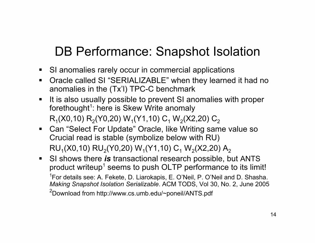
DB Performance: Snapshot Isolation SI anomalies rarely occur in commercial applications Oracle called SI “SERIALIZABLE” when they learned it had no

anomalies in the (Tx’l) TPC-C benchmark It is also usually possible to prevent SI anomalies with proper

forethought1: here is Skew Write anomalyR1(X0,10) R2(Y0,20) W1(Y1,10) C1 W2(X2,20) C2

Can “Select For Update” Oracle, like Writing same value soCrucial read is stable (symbolize below with RU)RU1(X0,10) RU2(Y0,20) W1(Y1,10) C1 W2(X2,20) A2

SI shows there is transactional research possible, but ANTSproduct writeup1 seems to push OLTP performance to its limit!1For details see: A. Fekete, D. Liarokapis, E. O’Neil, P. O’Neil and D. Shasha.Making Snapshot Isolation Serializable. ACM TODS, Vol 30, No. 2, June 20052Download from http://www.cs.umb.edu/~poneil/ANTS.pdf

15

DB Performance: Queries

Companies are spending the most money now ondeveloping query systems, with few, if any, updates

I’ll start with some historical development E. F. Codd’s Relational Paper was published in 1970;

Codd worked at IBM; DB2 was first released in 1982 SEQUEL, early SQL, was published1 in 1974 for

use in IBM’s System R, a DB2 precursor ORACLE (then Relational Software, Inc.) put out a

commercial version of SQL in 19791 Donald Chamberlin and Raymond Boyce, 1974. SEQUEL: A Structured English Query Language. SIGFIDET (later SIGMOD), pp. 249-264.

16

DB Performance: Early DB2 & M204 DB2 Query Indexes were explained in 1979 paper1

Rather primitive: Choose single column restriction that givessmallest “selectivity factor” F

Selectivity factor was later “Filter Factor” in documentation

The ability to AND Filter Factors waited until DB2 V2, 1988

After DB2 was introduced, Pat was working at CCA, which solda DBMS called Model 204 (M204) with efficient bitmap indexing

Pat published a paper called “The Set Query Benchmark”2 thatcompared M204 query performance to that of DB2 on MVS

Lucky that DB2 allowed this: DBMS products today would sue1P.G. Selinger et al., Access Path Selection in a relational database management system.SIGMOD 1979; 2 P. O'Neil. The Set Query Benchmark. Chapter 6 in The Benchmark Handbook forDatabase and Transaction Processing Systems. (1st Edition, 1989, 2nd Ed., 1993)

17

DB Performance: Set Query Benchmark Set Query Benchmark (SQB) has one table: BENCH (we tested

table join performance using self-joins on single BENCH table) BENCH table has 1,000,000 200-byte rows with a clustering

column KSEQ having sequential values 1, 2, . . ., 1,000,000 Also 12 random-valued columns, names indicating cardinality:

K2, K4, K5, K10, K25, K100, K1K, K10K, K100K, K250K, K500K E.g.: K10K has 10,000 values, each appearing randomly on

about 100 rows & K5 has 5 values, each on about 200,000 rows Additionally, 8 char string columns bring row up to 200 bytes Finally, we had 9 Query Suites providing “functional coverage”

of different forms of decision support in application use Each Suite has multiple queries with a range of different Filter

Factors (FFs) to provide “selectivity coverage”; SSB can be used asa “micro-benchmark” to predict performance of applications

Set Query Benchmark KNK columns

…

1

5

2

4

3

5

1

4

…

4523

0123

5790

0003

3457

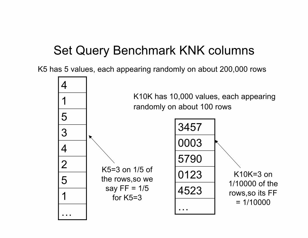
K5 has 5 values, each appearing randomly on about 200,000 rows

K10K has 10,000 values, each appearing randomly on about 100 rows

K5=3 on 1/5 ofthe rows,so wesay FF = 1/5

for K5=3

K10K=3 on1/10000 of therows,so its FF

= 1/10000

19

DB Performance: Set Query Benchmark Here is an example of Query Suite Q3B (underline: fix handout)

SELECT SUM(K1K) FROM BENCHWHERE (KSEQ between 400000 and 410000 OR KSEQ between 420000 and 430000

OR KSEQ between 440000 and 450000 OR KSEQ between 460000 and 470000OR KSEQ between 480000 and 500000) AND KN = 3; -- KN varies from K5 to K100K

---------------------------|==|---|==|---|==|---|==|---|==|==|--------------------------------------------------------- KSEQ-> 400000 500000 (midpoint in KSEQ)

This query sums dollar sales of a product of varying popularitysold in a given locale (thus in a broken range of zip codes)

DB2 and M204 both ran on IBM mainframe system MVS; Notethat the FF for KSEQ range is 0.06 and for KN = 3 is 1/CARD(KN)

DB2 did very well on queries requiring sequential or skip-sequential access to data (called sequential prefetch or list-prefetch by DB2), useful in Q3B

We wish to contrast performance in 1988-9 measurements ofMVS DB2 vs 2007 measurements of DB2 UDB on Windows

20

DB Performance: Set Query Comparison On Windows ran DB2 UDB on a 10,000,000 row BENCH table

using very fast modern system (very cheap compared to 1990) Query Plans for UDB same as MVS for KN = K100K, K10K & K5,

but different for KN = K100, K25 and K10

Composite FF for N = K10K is 0.06*(1/10,000) = 0.000006, so 6rows retrieved from MVS’s 1M, 62 rows from UDB’s 10M

KN UsedIn Q3B

Rows Read(of 1M)

DB2 MVS1M Rows

Index usage

DB2 UDB10M RowsIndex usage

DB2 MVS1M RowsTime secs

DB2 UDB10M RowsTime secs

K100K 1 K100 K100 1.4 0.7K10K 6 K10K K10K 2.4 3.1K100 597 K100, KSEQ KSEQ 14.9 2.1K25 2423 K25, KSEQ KSEQ 20.8 2.4K10 5959 K10, KSEQ KSEQ 31.4 2.3K5 12011 KSEQ KSEQ 49.1 2.1

Set Query Benchmark KNK index example

…

4523

0123

5790

0003

3457

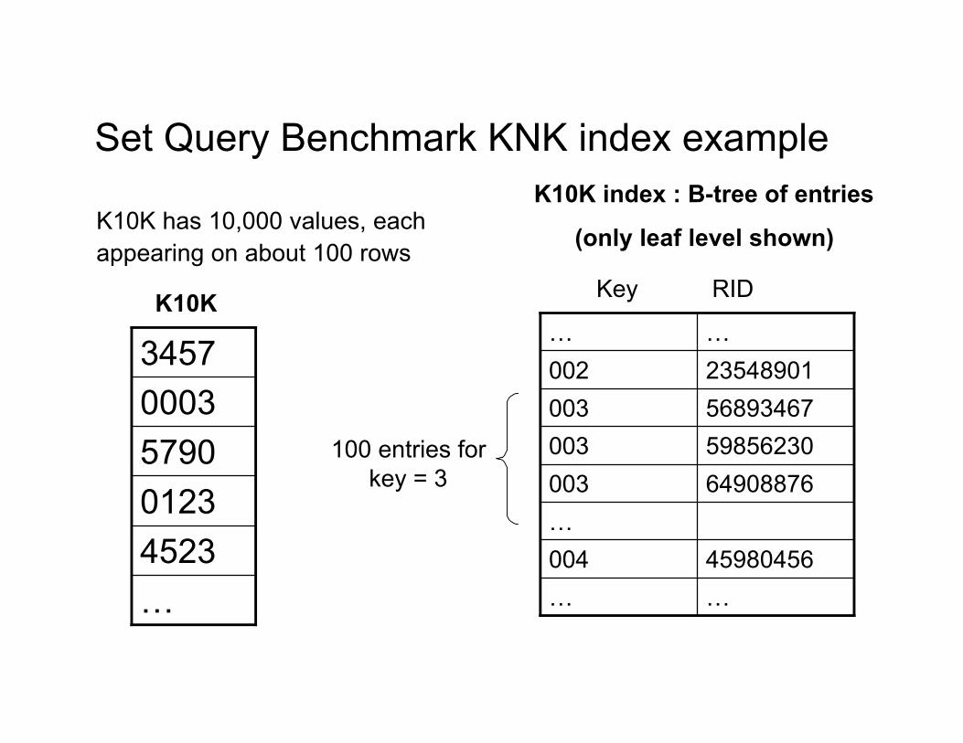
K10K has 10,000 values, each appearing on about 100 rows

45980456004

……

…

64908876003

59856230003

56893467003

23548901002

……

Key RID

100 entries forkey = 3

K10K

K10K index : B-tree of entries

(only leaf level shown)

22

DB Performance: Set Query Comparison For both DB2 MVS & DB2 UDB, Query Plan for KN = K100K &

K10K is: access rows with KN = 3 & test KSEQ in proper ranges DB2 MVS had .0001*(.06)*1,000,000 = 6 rows accessed for

K10K; DB2 UDB with 10,000,000 rows, had 62 rows accessed In these cases of very low selectivity, index driven access to

individual rows is still the best Query Plan

KN UsedIn Q3B

Rows Read(of 1M)

DB2 MVSIndex usage

DB2 UDBIndex usage

DB2 MVSTime secs

DB2 UDBTime secs

K100K 1 K100 K100 1.4 0.7K10K 6 K10K K10K 2.4 3.1

23

DB Performance: Set Query Comparison For KN = K100, K25 and K10, DB2 MVS ANDED KSEQ and

KN = 3 RID-lists, and accessed rows by RID to sum K1K values x x x x x x x x x x xx x x x x x x x x xx x x xx x x x|=====|———|=====|———|=====| ———|=====| ———|==========|

DB2 UDB on the other hand, scans each of five KSEQ rangesspecified & tests KN = 3 before summing K1K; DB2 MVS andDB2 UDB both use that same plan for K5 Scan&Tst Scan&Tst Scan&Tst Scan&Tst Scan and Test|=====|———|=====| ———|=====| ———|=====| ———|==========|

KN UsedIn Q3B

Rows Read(of 1M)

DB2 MVSIndex usage

DB2 UDBIndex usage

DB2 MVSTime secs

DB2 UDBTime secs

K100 597 K100, KSEQ KSEQ 14.9 2.1

K25 2423 K25, KSEQ KSEQ 20.8 2.4

K10 5959 K10, KSEQ KSEQ 31.4 2.3

K5 12011 KSEQ KSEQ 49.1 2.1

24

DB Performance: Set Query Comparison Both indexed retrieval of individual rows and sequential scan

have sped up since DB2 MVS, but sequential scan much more! Sequential scan speed has increased from MVS to UDB by a

factor of 88; random row retrieval speed by a factor of 4 FFs for speeding up random row retrieval are less important, but

clustering is more important: reduces sequential scan range

KN UsedIn Q3B

Rows Read(of 1M)

DB2 MVSIndex usage

DB2 UDBIndex usage

DB2 MVSTime secs

DB2 UDBTime secs

K100K 1 K100 K100 1.4 0.7K10K 6 K10K K10K 2.4 3.1K100 597 K100, KSEQ KSEQ 14.9 2.1K25 2423 K25, KSEQ KSEQ 20.8 2.4K10 5959 K10, KSEQ KSEQ 31.4 2.3K5 12011 KSEQ KSEQ 49.1 2.1

25

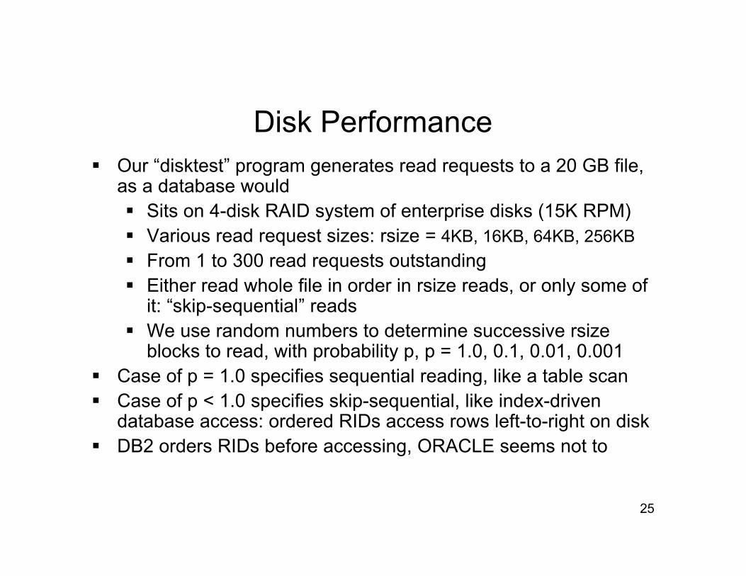
Disk Performance Our “disktest” program generates read requests to a 20 GB file,

as a database would Sits on 4-disk RAID system of enterprise disks (15K RPM) Various read request sizes: rsize = 4KB, 16KB, 64KB, 256KB

From 1 to 300 read requests outstanding Either read whole file in order in rsize reads, or only some of

it: “skip-sequential” reads We use random numbers to determine successive rsize

blocks to read, with probability p, p = 1.0, 0.1, 0.01, 0.001 Case of p = 1.0 specifies sequential reading, like a table scan Case of p < 1.0 specifies skip-sequential, like index-driven

database access: ordered RIDs access rows left-to-right on disk DB2 orders RIDs before accessing, ORACLE seems not to

26

Disk Performance

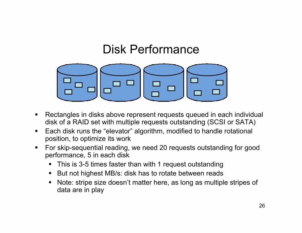
Rectangles in disks above represent requests queued in each individualdisk of a RAID set with multiple requests outstanding (SCSI or SATA)

Each disk runs the “elevator” algorithm, modified to handle rotationalposition, to optimize its work

For skip-sequential reading, we need 20 requests outstanding for goodperformance, 5 in each disk This is 3-5 times faster than with 1 request outstanding But not highest MB/s: disk has to rotate between reads Note: stripe size doesn’t matter here, as long as multiple stripes of

data are in play

27

Sequential Scan Performance Each disk can deliver 100MB/second with sequential scan

But throughput from disk to memory is limited by controller/bus

Disktest, reading sequentially, gets a maximum of 300MB/sec Need reads aligned to stripe boundaries to achieve maximum 300MB/sec

Our 4-disk RAID has 64KB stripe size, the Windows page I/O size

With 256KB reads (4 disk stripe set), only need 2 requests outstanding for300MB/sec

64KB reads (1 disk stripe at a time), 20 requests outstanding for 300MB/sec

Maximum read speed is not attainable with 4KB or 16KB reads

DBs get about 140 MB/second using tablescan (after tuning) Slowed down by needing to interpret data read in, extract rows, etc.

Need to tune DBs to use large reads, multiple outstanding reads

Oracle and Vertica recommend 1MB stripe size for DB RAID

28

Pointers on Setting up disks for DBs When experimenting, should partition RAID into (say) 5 parts Then can save tuned databases on different partitions Can reinitialize file system on old partition and copy data from

another; avoids file system fragmentation of multiple loads Can also build a new database on reinitialized partition Don’t worry about “raw disk”: current OS file I/O is great You will find that the lower-numbered partitions have faster

sequential reads, because of disk “zones” effect is about 30% for enterprise disks, more for cheap disks Just be aware of this effect, so you don’t misinterpret results

You can buy enterprise disks to use on an ordinary tower PC We used a Dell PowerEdge 2900, nice accessible internals Added SAS RAID controller, SAS disks

29

DB Performance:Outline of What Follows

First, we’ll examine Clustering historically, then a newDB2 concept of Multi-Dimensional Clustering (MDC)

We show how a form of MDC can be applied to otherDBMS products as well, e.g., Oracle, Sybase IQ

We want to apply this capability in the case of StarSchema Data Warehousing, but there’s a problem

We explain Star Schemas, and how the problem canbe addressed by Adjoined Dimension Columns

We introduce a “Star Schema Benchmark” and showperformance comparisons of three products

30

DB Performance: Linear Clustering Indexed clustering is an old idea; in 1980s one company had

demographic data on 80 million families from warranty cardsThey crafted mail lists for sales promotions of client companies

Typically, they concentrated on local areas (store localities) forthese companies to announce targeted sales: sports, toys, etc.

To speed searches, they kept families in order by zipcode; alsohad other data, so could restrict by incomeclass, hobbies, etc.

The result was something like like Q3B: a 50 mile radius circle ina state will result in a small union of ranges on zipcode

The Q3B range union was a fraction 0.06 of all possible valuesin clustering column KSEQ in BENCH

Clustered ranges are all the more important with modern disks

31

Multi-Dimensional Clustering Clustering by a single column of a table is fine if almost all

queries restrict by that column, but this is not always true DB2 was the first DBMS to provide a means of clustering by

more than one column at a time using MDC1

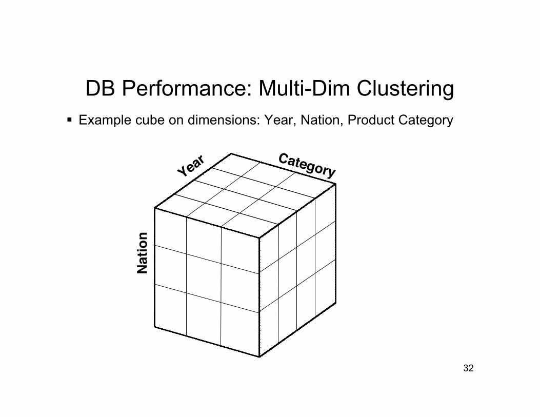
MDC partitions table data into Cells by treating some columnswithin the table as axes of a Cube

Each Cell in a Cube is defined by a combination of values inCube axis columns: Each row’s axis values define its Cell

New rows are placed in its Cell, which sits on a sequence ofBlocks on disk; Blocks must be large enough so sequential scanaccess speed on the cell swamps inter-cell access seek

Queries with multiple range predicates on axis columns willretrieve only data from Cells in range intersection

1S. Lightstone, T. Teory and T. Nadeau. Physical Database Design. Morgan Kaufmann

32

DB Performance: Multi-Dim Clustering Example cube on dimensions: Year, Nation, Product Category

Nation

CategoryYear

33

DB Performance: Multi-Dim Clustering Define DB2 MDC Cells in Create Table statement

create table Sales(units int, dollars decimal(9.2), prodid int, category int, nation char(12), selldate date, year smallint, . . .)

organize by dimensions (category, nation, year);

Cells on category, nation and year are created, sit on blocks

Each value of a dimension gives a Slice of the multi-dimensionalcube; has Block index entry listing BIDs of Blocks with that value

The BIDs in the intersection of all orthogonal Slices is for a Cell

DB2 supports Inserts of new rows of a table in MDC form; newrows are placed in some Block of the valid Cell, with new Blockadded if necessary; after Deletes, empty Blocks are freed

No guarantee Blocks for a Cell are near each other, but inter-block time swamped by speed of sequentially access to a block

MDC organization on disk

Example: MDC with three axes (AKA dimensions), nation,year, category, each with values 1, 2, 3, 4.

Let C123 stand for cell with axis values (1,2,3), I.e., nation =1, year = 2, category = 3

On disk, each block (1 MB say) belongs to a cell.

The sequence of blocks on disk is disordered:

C321 C411 C342 C433 C412 C143 C411 C231 C112 …

One cell, say C411, (nation = 4, year = 1, category = 1) hasseveral blocks,in different places, but since each block is 1MB, it’s worth a seek.

35

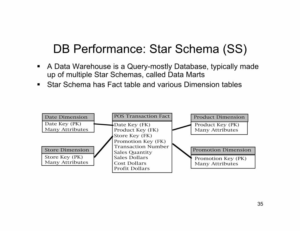
DB Performance: Star Schema (SS) A Data Warehouse is a Query-mostly Database, typically made

up of multiple Star Schemas, called Data Marts Star Schema has Fact table and various Dimension tables

Product Dimension

Product Key (PK) Many Attributes

Date DimensionDate Key (PK) Many Attributes

Promotion Dimension

Promotion Key (PK) Many Attributes

Store DimensionStore Key (PK) Many Attributes

Date Key (FK)Product Key (FK)Store Key (FK)Promotion Key (FK)Transaction NumberSales QuantitySales DollarsCost DollarsProfit Dollars

POS Transaction Fact

36

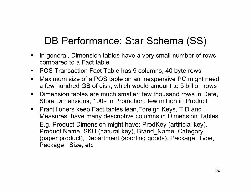
DB Performance: Star Schema (SS) In general, Dimension tables have a very small number of rows

compared to a Fact table POS Transaction Fact Table has 9 columns, 40 byte rows Maximum size of a POS table on an inexpensive PC might need

a few hundred GB of disk, which would amount to 5 billion rows Dimension tables are much smaller: few thousand rows in Date,

Store Dimensions, 100s in Promotion, few million in Product Practitioners keep Fact tables lean,Foreign Keys, TID and

Measures, have many descriptive columns in Dimension TablesE.g. Product Dimension might have: ProdKey (artificial key),Product Name, SKU (natural key), Brand_Name, Category(paper product), Department (sporting goods), Package_Type,Package _Size, etc

37

DB Performance: Data Warehousing Data Warehouse is made up of collection of Star Schemas often

representing supply chain on conforming dimensions1

1R. Kimball & M. Ross, The Data Warehouse Toolkit, 2nd Ed., Wiley

Retail Sales X X X X

Retail Inventory X X X

Retail Deliveries X X X

Warehouse Inventory X X X X

Warehouse Deliveries X X X X

Purchase Orders X X X X X X

Date

Prod

uct

Stor

ePr

omoti

onW

areh

ouse

Vend

orCo

ntrac

t

Etc.

Shipp

er

CONFORMING DIMENSIONS

SUPPLY CHAIN STAR SCHEMAS

38

DB Performance: Star Schema Queries Queries on Star Schemas typically retrieve aggregates of Fact

table measures (Sales Quantity/Dollars/Cost/Profit)

The Query Where Clauses typically restrict Dimension Columns:Product Category, Store Region, Month, etc.

Usually some Group By for Aggregation

Example Query 2.1 from Star Schema Benchmark (SSB):

select sum(lo_revenue), d_year, p_brand1from lineorder, date, part, supplierwhere lo_orderdate = d_datekey and lo_partkey = p_partkey

and lo_suppkey = s_suppkey and p_category = 'MFGR#12'and s_region = 'AMERICA'

group by d_year, p_brand1 order by d_year, p_brand1;

39

DB Performance: Multi-Dim Clustering Recall that DB2’s MDC treats table columns as orthogonal axes

of a Cube; these columns are called “Dimensions” But MDC “Dimensions” are columns in a table turned into a

Cube, not columns in Dimension tables of a Star Schema Of course we can’t embed all Dimension columns of a Star

Schema in the Fact table: would take up too much space forhuge number of rows

How does DB2 MDC handle Star Schemas? Not entirely clear For a foreign key of type Date a user can define a “generated

column” YearAndMonth mapped from Date by DB2; thiscolumn’s values can then be used to define MDC Cells

But not all Dimension columns can have generated columnsdefined on foreign keys: Product foreign key will not give brand

40

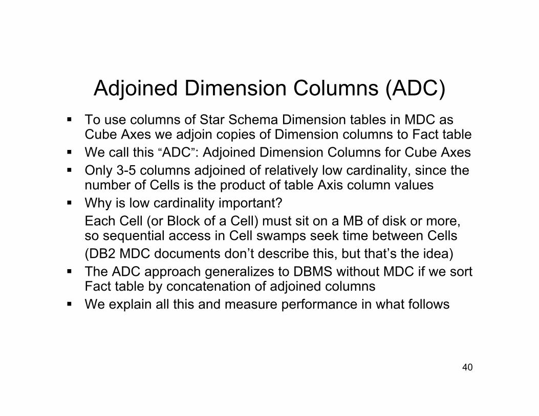
Adjoined Dimension Columns (ADC) To use columns of Star Schema Dimension tables in MDC as

Cube Axes we adjoin copies of Dimension columns to Fact table We call this “ADC”: Adjoined Dimension Columns for Cube Axes Only 3-5 columns adjoined of relatively low cardinality, since the

number of Cells is the product of table Axis column values Why is low cardinality important?

Each Cell (or Block of a Cell) must sit on a MB of disk or more,so sequential access in Cell swamps seek time between Cells(DB2 MDC documents don’t describe this, but that’s the idea)

The ADC approach generalizes to DBMS without MDC if we sortFact table by concatenation of adjoined columns

We explain all this and measure performance in what follows

41

ADC: Outline of What Follows

ADC works well with DB2 MDC or Oracle partitions oreven a DBMS that simply has good indexing

ADC can have problems with inserts to the base tableif Cells are not defined on a Materialized View

We will measure performance using a Star Schemabenchmark (SSB): The SSB schema is defined as atransformation of a TPC-H benchmark schema

We analyze SSB Queries by clustering performed:Cluster Factor (CF) instead of Filter Factor (FF)

Then we provide experimental results, furtheranalysis, and conclusions

42

Adjoining Dimension Columns: Example

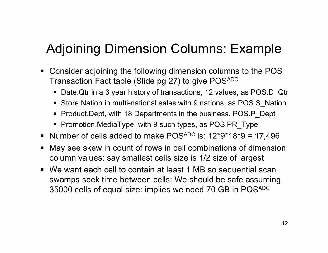
Consider adjoining the following dimension columns to the POSTransaction Fact table (Slide pg 27) to give POSADC

Date.Qtr in a 3 year history of transactions, 12 values, as POS.D_Qtr

Store.Nation in multi-national sales with 9 nations, as POS.S_Nation

Product.Dept, with 18 Departments in the business, POS.P_Dept

Promotion.MediaType, with 9 such types, as POS.PR_Type

Number of cells added to make POSADC is: 12*9*18*9 = 17,496

May see skew in count of rows in cell combinations of dimensioncolumn values: say smallest cells size is 1/2 size of largest

We want each cell to contain at least 1 MB so sequential scanswamps seek time between cells: We should be safe assuming35000 cells of equal size: implies we need 70 GB in POSADC

43

Adjoining Dimension Columns

Note that POSADC is not a materialized view of POS in alldatabase system products; there will be two separate tables

Given a row for insert in POS, we use foreign keys in the row todetermine ADC column values for insert in POSADC

Thus we give up on working with POS to deal with POSADC

unless we always insert new rows in both POS and POSADC

Vertica1 DBMS supports ordered materialized views created fromjoins of tables: we’ll see why ordering can be important shortly

1C-Store, A Column-Oriented DBMS, M. Stonebraker et al. http://db.csail.mit.edu/projects/cstore/vldb.pdf

44

Considerations and Futures of ADC

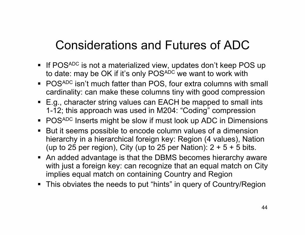
If POSADC is not a materialized view, updates don’t keep POS upto date: may be OK if it’s only POSADC we want to work with

POSADC isn’t much fatter than POS, four extra columns with smallcardinality: can make these columns tiny with good compression

E.g., character string values can EACH be mapped to small ints1-12; this approach was used in M204: “Coding” compression

POSADC Inserts might be slow if must look up ADC in Dimensions But it seems possible to encode column values of a dimension

hierarchy in a hierarchical foreign key: Region (4 values), Nation(up to 25 per region), City (up to 25 per Nation): 2 + 5 + 5 bits.

An added advantage is that the DBMS becomes hierarchy awarewith just a foreign key: can recognize that an equal match on Cityimplies equal match on containing Country and Region

This obviates the needs to put “hints” in query of Country/Region

45

Compressing ADC

Won’t have all tricks of prior slide in any current DBMS But we can usually compress adjoined dimension columns to

small ints: use UDF for mapping so Store.Nation = ‘UnitedStates’ maps to small int 7

create function NATcode (nat char(18)) returns small int…return case nat

when ‘United Kingdom’ then 1…when ‘United States’ then 7…

end

Now a user can write:Select … from POS where S_Nation = Natcode(‘United States’)…

Natcode will translate ‘United States’ to the int 7; thus all ADCcan be two-byte (or less) small ints with proper UDFs defined

46

Using ADC With Oracle

Oracle has a feature “Partitioning” that corresponds to DB2 MDC Given ADCs C1, C2, C3 and C4, create Cells of a Cube using the

Partition clause in Create Table on a concatenation of thesecolumns (assume values for columns are 0, 1 & 2, for illustration)

…partition C0001 values less than (0,0,0,1) tablespace TS1partition C0002 values less than (0,0,0,2) tablespace TS1partition C0010 values less than (0,0,1,0) tablespace TS1 -- (0,0,1,0) next after (0,0,0,2)…partition C1000 values less than (1,0,0,0) tablespace TS2

… -- NOTE: Inserts of new rows also work with partitioning

Map Dimension value to number, Oracle compresses to byte if fitscreate or replace function natcode (nat char(18)) return number isbegin

return case natwhen ‘United Kingdom’ then 1…

47

Create Cells Using Table Order & ADC

For DBMS with good indexing, define Cells by concatenating (4)Adjoined Dimension Columns and sorting table by this order

Each cell represents unique combination of ADC values (2,7,4,3)

A Where clause with ANDed range predicates on four ADCs, each rangeover 3 ADC values, will select 81 cells on the table

Cells Selected will not sit close to each other, except for cells differingonly in the final ADC values, e.g.: (2,7,4,3) and (2,7,4,4)

Obviously this approach doesn’t allow later inserts into given cells

The Vertica DBMS uses this approach, but since new inserts go intoWOS in memory, later merged out to disk ROS, new ad hoc inserts AREpossible

48

Star Schema Benchmark (SSB)

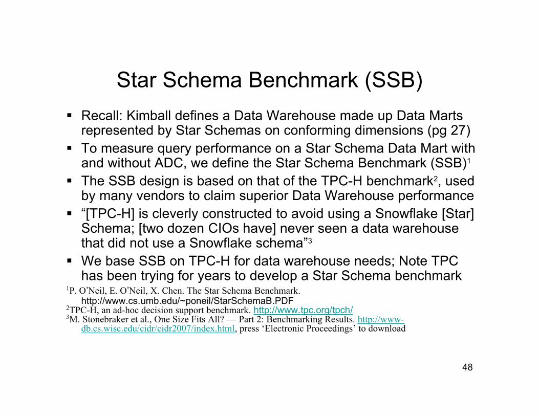
Recall: Kimball defines a Data Warehouse made up Data Martsrepresented by Star Schemas on conforming dimensions (pg 27)

To measure query performance on a Star Schema Data Mart withand without ADC, we define the Star Schema Benchmark (SSB)1

The SSB design is based on that of the TPC-H benchmark2, usedby many vendors to claim superior Data Warehouse performance

“[TPC-H] is cleverly constructed to avoid using a Snowflake [Star]Schema; [two dozen CIOs have] never seen a data warehousethat did not use a Snowflake schema”3

We base SSB on TPC-H for data warehouse needs; Note TPChas been trying for years to develop a Star Schema benchmark

1P. O’Neil, E. O’Neil, X. Chen. The Star Schema Benchmark.http://www.cs.umb.edu/~poneil/StarSchemaB.PDF

2TPC-H, an ad-hoc decision support benchmark. http://www.tpc.org/tpch/3M. Stonebraker et al., One Size Fits All? — Part 2: Benchmarking Results. http://www-

db.cs.wisc.edu/cidr/cidr2007/index.html, press ‘Electronic Proceedings’ to download

49

Star Schema Benchmark (SSB)Created to Measure Star Schema Query Performance

50

SSB is Derived From TPC-H BenchmarkPARTKEY

PART (P_)SF*200,000

NAME

MFGR

BRAND

TYPE

SIZE

CONTAINER

RETAILPRICE

COMMENT

SUPPLIER (S_) SF*10,000SUPPKEY

NAME

ADDRESS

NATIONKEY

PHONE

ACCTBAL

COMMENT

PARTSUPP (PS_) SF*800,000

PARTKEY

SUPPKEY

AVAILQTY

SUPPLYCOST

COMMENT

CUSTOMER (C_) SF*150,000CUSTKEY

NAME

ADDRESS

NATIONKEY

PHONE

ACCTBAL

MKTSEGMENT

COMMENT

CUSTKEY

NAME

NAMECOMMENT

COMMENT

COMMENT

COMMENT

NATIONKEY

NATION (N_) 25

REGIONKEY REGIONKEY

LINEITEM (L_)SF*6,000,000ORDERKEY

LINENUMBER

QUANTITY

EXTENDED-PRICE

DISCOUNT

TAX

RETURNFLAG

LINESTATUS

SHIPDATE

COMMITDATE

RECEIPTDATE

SHIPINSTRUCT

SHIPMODE

PARTKEY

SUPPKEY

REGION (R_) 5

ORDERKEY

ORDERS (O_)SF*1,500,000

ORDERSTATUS

TOTALPRICE

ORDERDATE

ORDER-PRIORITY

CLERK

SHIP-PRIORITY

51

Why Changes to TPC-H Make Sense

TPC-H has PARTSUPP table listing Suppliers of ordered Parts toprovide information on SUPPLYCOST and AVAILQTY

This is silly: there are seven years of orders (broken into ORDERSand LINEITEM table) and SUPPLYCOST not stable for that period

PARTSUPP looks like OLTP, not a Query table: as I fill orders Iwould want to know AVAILQTY, but meaningless over 7 years?

AVAILQTY and SUPPLYCOST are never Refressed in TPC-Heither; We say PARTSUPP has the wrong temporal “granularity”1

One suspects the real reason for PARTSUPP is to break up whatwould be a Star Schema, so Query Plans become harderCombining LINEITEM and ORDER in TPC-H to get LINEORDER inSSB, with one row for each one in LINEITEM, is common practice1

1The Data Warehouse Toolkit, 2nd Ed, Ralph Kimball and Margy Ross. Wiley

52

Why Changes to TPC-H Make Sense

To take the place of PARTSUPP, we have a column SUPPLYCOSTin LINEORDER of SSB to give cost of each item when ordered

Note that a part order might be broken into two or more lineitemsof the order if lowest cost supplier didn’t have enough parts

Another modification of TPC-H for SSB was that TPC-H columnsSHIPDATE, RECEIPTDATE and RETURNFLAG were all droppedThis information isn’t known until long after the order is placed;we kept ORDERDATE and COMMITDATE (the commit date is acommitment made at order time as to when shipment will occur)One would typically need multiple star schemas to contain otherdates from TPC-H, and we didn’t want SSB that complicated

A number of other modifications were made; for a complete list,see: http://www.cs.umb.edu/~poneil/StarSchemaB.PDF

53

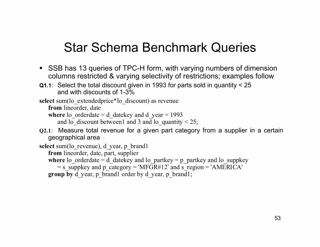
Star Schema Benchmark Queries

SSB has 13 queries of TPC-H form, with varying numbers of dimensioncolumns restricted & varying selectivity of restrictions; examples follow

Q1.1: Select the total discount given in 1993 for parts sold in quantity < 25and with discounts of 1-3%

select sum(lo_extendedprice*lo_discount) as revenuefrom lineorder, datewhere lo_orderdate = d_datekey and d_year = 1993

and lo_discount between1 and 3 and lo_quantity < 25;Q2.1: Measure total revenue for a given part category from a supplier in a certain

geographical areaselect sum(lo_revenue), d_year, p_brand1

from lineorder, date, part, supplierwhere lo_orderdate = d_datekey and lo_partkey = p_partkey and lo_suppkey

= s_suppkey and p_category = 'MFGR#12’ and s_region = 'AMERICA'group by d_year, p_brand1 order by d_year, p_brand1;

54

Star Schema Benchmark Queries

Successive Queries in a flight (Q1.2, Q1.3 in flight Q1) use tighterrestrictions to reduce Where clause selectivity

Q1.1:Select the total discount given in 1993 for parts sold in quantity < 25and with discounts of 1-3%

select sum(lo_extendedprice*lo_discount) as revenuefrom lineorder, datewhere lo_orderdate = d_datekey and d_year = 1993

and lo_discount between1 and 3 and lo_quantity < 25;

Q1.3: Same as Q1.1, except parts sold in smaller range and date limited toone week

select sum(lo_extendedprice*lo_discount) as revenuefrom lineorder, datewhere lo_orderdate = d_datekey and d_weeknuminyear = 6 and d. year = 1994

and lo_discount between 5 and 7 and lo_quantity between 25 and 35

See list of queries starting on page 9 of ADC Index preprint handout

55

Star Schema Benchmark Cluster Factors

Query CF onlineorder

CFs of indexable predicateson dimension columns

Combined CF Effecton lineorder

CF ondiscount& quantity

CF onDate

CF onpartBrand1roll-up

CF onsuppliercity roll-up

CF oncustomercity roll-up

Q1.1 .47*3/11 1/7 .019Q1.2 .2*3/11 1/84 .00065Q1.3 .1*3/11 1/364 .000075Q2.1 1/25 1/5 1/125 = .0080Q2.2 1/125 1/5 1/625 = .0016Q2.3 1/1000 1/5 1/5000 = .00020Q3.1 6/7 1/5 1/5 6/175 = .034Q3.2 6/7 1/25 1/25 6/4375 = .0014Q3.3 6/7 1/125 1/125 6/109375 =.000055Q3.4 1/84 1/125 1/125 1/1312500= .000000762Q4.1 2/5 1/5 1/5 2/125 = .016Q4.2 2/7 2/5 1/5 1/5 4/875 = .0046Q4.3 2/7 1/25 1/25 1/5 2/21875 = .000091

56

SSB Test Specifications

We measured three DB products we call A, B, and C, using SSBtables at Scale Factor 10, where LINEORDER has about 6 GB

Tests were performed on a Dell 2900 running Windows Server2003, with 8 GB of RAM (all queries had cold starts), two 64-bitdual core processors (3.2 GHz each), and data loaded on RAID0with 4 Seagate 15000 RPM SAS disks (136 GB each), with stripesize 64 KB This is a fast system in current terms;

We had to experiment to find good tuning settings for number ofreads outstanding: parallel threads, prefetching

Adjoined dimension columns were d.year, s.region, c.region, andp.category (brand-hierarchy), cardinalities 7, 5, 5, and 25

In LINEORDER table these adjoined columns were named year,sregion, cregion, category, and used in the SSB Queries

57

SSB Load

We performed two loads for DBs A, B and C, one with adjoined columnsand one with no adjoined columns, called BASIC form

First we generated rows of SSB LINEORDER and dimensions usinggenerator that populates TPC-H, with needed modifications

After loading LINEORDER in Basic form, used a query (below) to outputthe data with adjoined columns in order by concatenation; could use thisorder to load DB with indexing, or to help speed up DB2 MDC load andOracle Partition load

select L.*, d_year, s_region, c_region, p_categoryfrom lineorder, customer, supplier, part, datewhere lo_custkey = c_custkey and lo_suppkey = s_suppkey

and lo_partkey = p_partkey and lo_datekey = d_datekeyorder by d_year, s_region, c_region, p_category;

58

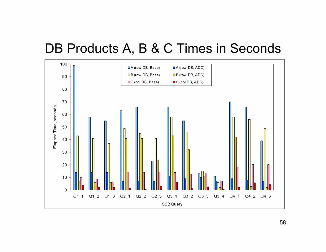
DB Products A, B & C Times in Seconds

59

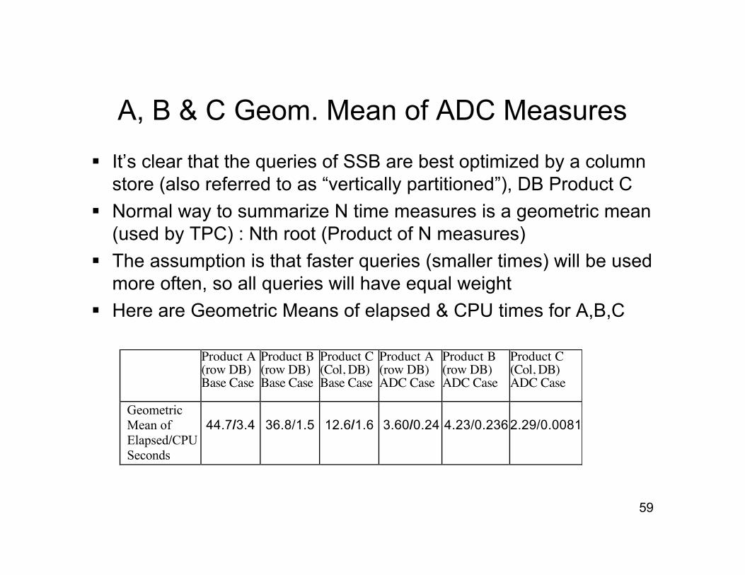
A, B & C Geom. Mean of ADC Measures

It’s clear that the queries of SSB are best optimized by a columnstore (also referred to as “vertically partitioned”), DB Product C

Normal way to summarize N time measures is a geometric mean(used by TPC) : Nth root (Product of N measures)

The assumption is that faster queries (smaller times) will be usedmore often, so all queries will have equal weight

Here are Geometric Means of elapsed & CPU times for A,B,C

Product A(row DB)Base Case

Product B(row DB)Base Case

Product C(Col, DB)Base Case

Product A(row DB)ADC Case

Product B(row DB)ADC Case

Product C(Col, DB)ADC Case

GeometricMean ofElapsed/CPUSeconds

44.7/3.4 36.8/1.5 12.6/1.6 3.60/0.24 4.23/0.2362.29/0.0081

60

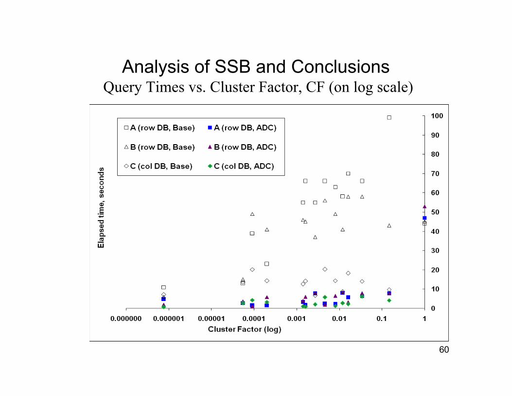
Analysis of SSB and Conclusions Query Times vs. Cluster Factor, CF (on log scale)

61

Analysis of SSB and Conclusions

On plot of slide 56, differentiate three regions of cluster factor: CF

At low end of the CF Axis (CF < 1/10000), secondary indexes areeffective at retrieving few rows qualified: ADC has little advantage

For CF up near 1.0, the whole table is read with sequential scanregardless of ADC, and the times again group together

For CF in the intermediate range where most queries lie, ADC reducesquery times very effectively compared to the BASE case

Time is reduced from approximately that required for a sequential scandown to a few seconds (at most ten seconds)

We believe this demonstrates the validity of our ADC approach

62

Analysis and Conclusions

Readers should bear in mind that the Star Schema Benchmark has quitesmall dimensions, with rather simple rollup hierarchies

With more complex dimensions and query workloads in largecommercial applications, no single ADC choice will speed up all possiblequeries

Of course this has always been the case with clustering solutions: theynever improve performance of all possible queries

Still, there are many commercial data warehouse applications whereclustering of this sort should be an invaluable aid

63

BibliographyH. Berenson, P Bernstein, J. Gray, J. Melton, P. O’Neil, E. O’Neil, A Critique of

ANSI Isolation Levels. SIGMOD 2005.

D. Chamberlin and R. Boyce, SEQUEL: A Structured English Query Language.SIGFIDET 1974 (later SIGMOD), pp. 249-264.

A. Fekete, D. Liarokapis, E. O’Neil, P. O’Neil and D. Shasha. Making SnapshotIsolation Serializable. ACM TODS, Vol 30, No. 2, June 2005

Jim Gray, ed., The Benchmark Handbook, in ACM SIGMOD Anthology,http://www.sigmod.org/dblp/db/books/collections/gray93.html

R. Kimball & M. Ross, The Data Warehouse Toolkit, 2nd Ed., Wiley, 2002

S. Lightstone, T. Teory and T. Nadeau. Physical Database Design, MorganKaufmann, 2007

P. O’Neil, E. O’Neil, X. Chen. The Star Schema Benchmark.http://www.cs.umb.edu/~poneil/StarSchemaB.PDF

64

BibliographyP.G. Selinger et al., Access Path Selection in a relational database

management system. SIGMOD 1979;

M. Stonebraker et al, C-Store, A Column-Oriented DBMS, VLDB 2005.http://db.csail.mit.edu/projects/cstore/vldb.pdf

M. Stonebraker et al., One Size Fits All? — Part 2: Benchmarking Results.CIDR 2007 http://www-cs.wisc.edu/cidr/cidr2007/index.html, press‘Electronic Proceedings’ to download

TPC-H, an ad-hoc decision support benchmark. http://www.tpc.org/tpch/