Sirindhorn International Institute of Technology

Thammasat University

School of Information, Computer and Communication Technology

ECS332 2015/1 Part I Dr.Prapun

1 Introduction to communication systems

1.1. Shannon’s insight [8]:

The fundamental problem of communication is that of reproducingat one point either exactly or approximately a message selected atanother point.

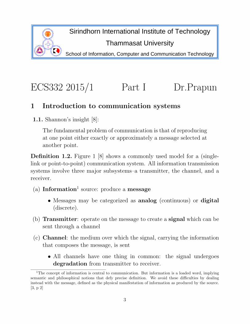
Definition 1.2. Figure 1 [8] shows a commonly used model for a (single-link or point-to-point) communication system. All information transmissionsystems involve three major subsystems–a transmitter, the channel, and areceiver.

(a) Information1 source: produce a message

• Messages may be categorized as analog (continuous) or digital(discrete).

(b) Transmitter: operate on the message to create a signal which can besent through a channel

(c) Channel: the medium over which the signal, carrying the informationthat composes the message, is sent

• All channels have one thing in common: the signal undergoesdegradation from transmitter to receiver.

1The concept of information is central to communication. But information is a loaded word, implyingsemantic and philosophical notions that defy precise definition. We avoid these difficulties by dealinginstead with the message, defined as the physical manifestation of information as produced by the source.[3, p 2]

3

Although this degradation may occur at any point of the com-munication system block diagram, it is customarily associatedwith the channel alone.

This degradation often results from noise2 and other unde-sired signals or interference3 but also may include other dis-tortion4 effects as well, such as fading signal levels, multipletransmission paths, and filtering.

(d) Receiver: transform the signal back into the message intended fordelivery

(e) Destination: a person or a machine, for whom or which the messageis intended

Basic elements of communication

29

Information source: produce a message

Transmitter: operate on the message to create a signal which can be sent through a channel

Noise Source

Receiver Transmitter Information

Source Destination Channel

Received

Signal Transmitted

Signal Message Message

Figure 1: Schematic diagram of a general communication system

2Noise refers to random and unpredictable electrical signals produced by natural processes both internaland external to the system. [3, p 4]

3Interference is contamination by extraneous signals from human sourcesother transmitters, power linesand machinery, switching circuits, and so on. Interference occurs most often in radio systems whosereceiving antennas usually intercept several signals at the same time. [3, p 4]

4Distortion is waveform perturbation caused by imperfect response of the system to the desired signalitself. Unlike noise and interference, distortion disappears when the signal is turned off. If the channel hasa linear but distorting response, then distortion may be corrected, or at least reduced, with the help ofspecial filters called equalizers. [3, p 4]

4

2 Frequency-Domain Analysis

Electrical engineers live in the two worlds, so to speak, of time and frequency.Frequency-domain analysis is an extremely valuable tool to the communi-cations engineer, more so perhaps than to other systems analysts. Since thecommunications engineer is concerned primarily with signal bandwidths andsignal locations in the frequency domain, rather than with transient analysis,the essentially steady-state approach of the (complex exponential) Fourierseries and transforms is used rather than the Laplace transform.

2.1 Math background

2.1. Euler’s formula :

ejx = cosx+ j sinx. (1)

cos (A) = ReejA

=1

2

(ejA + e−jA

)(2)

sin (A) = ImejA

=1

2j

(ejA − e−jA

). (3)

2.2. We can use cosx = 12

(ejx + e−jx

)and sinx = 1

2j

(ejx − e−jx

)to derive

many trigonometric identities. See Example 2.4.

Example 2.3. Use the Euler’s formula to show that ddx sinx = cosx.

Example 2.4. Use the Euler’s formula to show that cos2(x) = 12 (cos(2x) + 1).

5

2.5. Similar technique gives

(a) cos(−x) = cos(x),

(b) cos(x− π

2

)= sin(x),

(c) sin2x = 12 (1− cos (2x))

(d) sin(x) cos(x) = 12 sin(2x), and

(e) the product-to-sum formula

cos(x) cos(y) =1

2(cos(x+ y) + cos(x− y)) . (4)

2.2 Continuous-Time Fourier Transform

Definition 2.6. The (direct) Fourier transform of a signal g(t) is definedby

G(f) =

+∞∫−∞

g(t)e−j2πftdt (5)

This provides the frequency-domain description of g(t). Conversion back tothe time domain is achieved via the inverse (Fourier) transform:

g (t) =

∞∫−∞

G (f) ej2πftdf (6)

• We may combine (5) and (6) into one compact formula:

∞∫−∞

G (f) ej2πftdf = g (t)F−−−−F−1

G (f) =

∞∫−∞

g (t) e−j2πftdt. (7)

• We may simply write G = F g and g = F−1 G.

• Note that G(0) =∫∞−∞ g(t)dt and g(0) =

∫∞−∞G(f)df .

6

2.7. In some references5, the (direct) Fourier transform of a signal g(t) isdefined by

G(ω) =

∫ +∞

−∞g(t)e−jωtdt (8)

In which case, we have

1

2π

∞∫−∞

G (ω) ejωtdω = g (t)F−−−−F−1

G (ω) =

∞∫−∞

g (t) e−jωtdt (9)

• In MATLAB, these calculations are carried out via the commands fourierand ifourier.

• Note that G(0) =∞∫−∞

g(t)dt and g(0) = 12π

∞∫−∞

G(ω)dω.

• The relationship between G(f) in (5) and G(ω) in (8) is given by

G(f) = G(ω)∣∣∣ω=2πf

(10)

G(ω) = G(f)|f= ω2π

(11)

Before we introduce our first but crucial transform pair in Example 2.12which will involve rectangular function, we want to introduce the indicatorfunction which gives compact representation of the rectangular function.We will see later that the transform of the rectangular function gives a sincfunction. Therefore, we will also introduce the sinc function as well.

Definition 2.8. An indicator function gives only two values: 0 or 1. Itis usually written in the form

1[some condition(s) involving t].

Its value at a particular t is one if and only if the condition(s) inside issatisfied for that t. For example,

1[|t| ≤ a] =

1, −a ≤ t ≤ a,

0, otherwise.

5MATLAB uses this definition.

7

Alternatively, we can use a set to specify the values of t at which the indi-cator function gives the value 1:

1A(t) =

1, t ∈ A,0, t /∈ A.

In particular, the set A can be some intervals:

1[−a,a](t) =

1, −a ≤ t ≤ a,0, otherwise,

and

1[−a,b](t) =

1, −a ≤ t ≤ b,0, otherwise.

Example 2.9. Carefully sketch the function g(t) = 1 [|t| ≤ 5]

Definition 2.10. Rectangular pulse [3, Ex 2.21 p 45]:

•∏

(t) = 1 [|t| ≤ 0.5] = 1[−0.5,0.5] (t)

This is a pulse of unit height and unit width, centered at the origin.Hence, it is also known as the unit gate function rect (x) [4, p 78].

In [3], the values of the pulse∏

(t) at 0.5 and−0.5 are not specified.However, in [4], these values are defined to be 0.5.

In MATLAB, the function rectangularPulse(t) can be used to pro-duce6 the unit gate function above. More generally, we can producea rectangular pulse whose rising edge is at a and falling edge is atb via rectangularPulse(a,b,t).

•∏(

tT0

)= 1

[|t| ≤ T0

2

]= 1[−T02 ,

T02 ] (t)

Observe that T0 is the width of the pulse.

6Note that rectangularPulse(-0.5) and rectangularPulse(0.5) give 0.5 in MATLAB.

8

Definition 2.11. The function

sinc(x) ≡ (sinx)/x (12)

is plotted in Figure 2.

sinc function

50

0 2-

1

-0.2172

0.1284

-0.0913

sinc

1/1/

cos sin

Figure 2: Sinc function

• This function plays an important role in signal processing. It is alsoknown as the filtering or interpolating function.

The full name of the function is “sine cardinal”7.

• Using L’Hopital’s rule, we find limx→0

sinc(x) = 1.

• sinc(x) is the product of an oscillating signal sin(x) (of period 2π) anda monotonically decreasing function 1/x . Therefore, sinc(x) exhibitssinusoidal oscillations of period 2π, with amplitude decreasing contin-uously as 1/x.

• Its zero crossings are at all non-zero integer multiples of π.

7which corresponds to the Latin name sinus cardinalis. It was introduced by Woodward in his 1952paper “Information theory and inverse probability in telecommunication” [10], in which he noted that it“occurs so often in Fourier analysis and its applications that it does seem to merit some notation of itsown”

9

• In MATLAB, in [3, p 37], in [12, eq. 2.64], and in [10], sinc(x) is defined as(sin(πx))/πx. In which case, its zero crossings are at non-zero integervalues of its argument.

This is sometimes called the “normalized” sinc function to distin-guish it from (12) which is unnormalized .

Example 2.12. Rectangular function and Sinc function:

1 [|t| ≤ a]F−−−−F−1

sin(2πfa)

πf=

2 sin (aω)

ω= 2a sinc (aω) (13)

( )0sinc 2 f tπ

1

0

12 f

0

1f

1−

F

F t

00

1 1 22

ff

ω π⎡ ≤ ⎤⎣ ⎦

02 fπ

ω 0

12 f

0f

f 0

12 f

1−

F

F

00sinc

2TT ω⎛ ⎞⎜ ⎟⎝ ⎠

0T

0

2Tπ

ω

t ( )0 0sincT T fπ

0T

0

1T

f

1

0

2T 0

2T

−

0T

Figure 3: Fourier transform of sinc and rectangular functions

By setting a = T0/2, we have

1

[|t| ≤ T0

2

]F−−−−F−1

T0 sinc(πT0f). (14)

In particular, when T0 = 1, we have rect (t)F−−−−F−1

sinc(πt). The Fourier

transform of the unit gate function is the normalized sinc function.

10

Definition 2.13. The (Dirac) delta function or (unit) impulse func-tion is denoted by δ(t). It is usually depicted as a vertical arrow at theorigin. Note that δ(t) is not8 a true function; it is undefined at t = 0. Wedefine δ(t) as a generalized function which satisfies the sampling property(or sifting property) ∫ ∞

−∞φ(t)δ(t)dt = φ(0) (15)

for any function φ(t) which is continuous at t = 0.

• In this way, the delta “function” has no mathematical or physical mean-ing unless it appears under the operation of integration.

• Intuitively we may visualize δ(t) as an infinitely tall, infinitely narrowrectangular pulse of unit area: lim

ε→0

1ε1[|t| ≤ ε

2

].

2.14. Properties of δ(t):

• δ(t) = 0 for t 6= 0.δ(t− T ) = 0 for t 6= T .

•∫A δ(t)dt = 1A(0).

(a)∫∞−∞ δ(t)dt = 1.

(b)∫0 δ(t)dt = 1.

(c)∫ x−∞ δ(t)dt = 1[0,∞)(x). Hence, we may think of δ(t) as the “deriva-

tive” of the unit step function U(t) = 1[0,∞)(x) [11, Defn 3.13 p126].

•∫∞−∞ g(t)δ(t− c)dt = g(c) for g continuous at T . In fact, for any ε > 0,∫ T+ε

T−εgt)δ(t− c)dt = g(c).

• Convolution9 property:

(δ ∗ g)(t) = (g ∗ δ)(t) =

∫ ∞−∞

g(τ)δ(t− τ)dτ = φ(t) (16)

where we assume that φ is continuous at t.8The δ-function is a distribution, not a function. In spite of that, it’s always called δ-function.9See Definition 2.34.

11

• δ(at) = 1|a|δ(t). In particular,

δ(ω) =1

2πδ(f) (17)

and

δ(ω − ω0) = δ(2πf − 2πf0) =1

2πδ(f − f0), (18)

where ω = 2πf and ω0 = 2πf0.

Example 2.15.2∫−1

δ (t)dt = and2∫

1

δ (t)dt = .

Example 2.16.2∫

0

δ (t)dt =

Example 2.17. δ(t)F−−−−F−1

1.

Example 2.18. ej2πf0tF−−−−F−1

δ (f − f0).

Example 2.19. ejω0tF−−−−F−1

2πδ (ω − ω0).

Example 2.20. ej4πtF−−−−F−1

12

Example 2.21. cos(200πt)F−−−−F−1

2.22. cos(2πf0t)F−−−−F−1

12 (δ (f − f0) + δ (f + f0)).

Example 2.23. cos(200t)F−−−−F−1

Example 2.24. cos (200πt) + cos (400πt)F−−−−F−1

Example 2.25. cos (t)− 13 cos (3t) + 1

5 cos (5t)F−−−−F−1

Fourier transform: Example

1

cos13 cos 3

15 cos 5

f

12

12

16

16

110

110

t

t

Example 2.26. cos2 (200πt)F−−−−F−1

13

Example 2.27. cos (200πt)× cos (400πt)F−−−−F−1

2.28. Conjugate symmetry10: If g(t) is real-valued, then G(−f) =(G(f))∗

(a) Even amplitude symmetry: |G (−f)| = |G (f)|

(b) Odd phase symmetry: ∠G (−f) = −∠G (f)

Observe that if we know X(f) for all f positive, we also know X(f) forall f negative. Interpretation: Only half of the spectrum contains allof the information. Positive-frequency part of the spectrum contains allthe necessary information. The negative-frequency half of the spectrum canbe determined by simply complex conjugating the positive-frequency half ofthe spectrum.

Furthermore,

(a) If g(t) is real and even, then so is G(f).

(b) If g(t) is real and odd, then G(f) is pure imaginary and odd.

10Hermitian symmetry in [3, p 48] and [7, p 17 ].

14

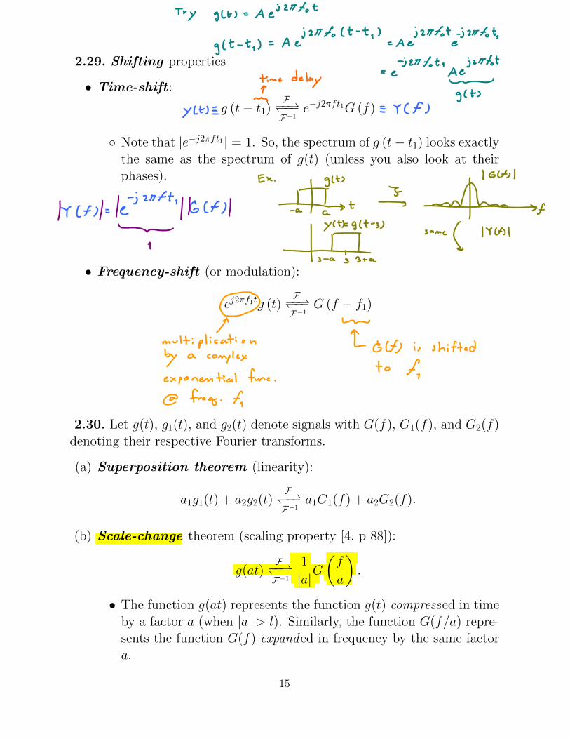
2.29. Shifting properties

• Time-shift :

g (t− t1)F−−−−F−1

e−j2πft1G (f)

Note that |e−j2πft1| = 1. So, the spectrum of g (t− t1) looks exactlythe same as the spectrum of g(t) (unless you also look at theirphases).

• Frequency-shift (or modulation):

ej2πf1tg (t)F−−−−F−1

G (f − f1)

2.30. Let g(t), g1(t), and g2(t) denote signals with G(f), G1(f), and G2(f)denoting their respective Fourier transforms.

(a) Superposition theorem (linearity):

a1g1(t) + a2g2(t)F−−−−F−1

a1G1(f) + a2G2(f).

(b) Scale-change theorem (scaling property [4, p 88]):

g(at)F−−−−F−1

1

|a|G

(f

a

).

• The function g(at) represents the function g(t) compressed in timeby a factor a (when |a| > l). Similarly, the function G(f/a) repre-sents the function G(f) expanded in frequency by the same factora.

15

• The scaling property says that if we “squeeze” a function in t,its Fourier transform “stretches out” in f . It is not possible toarbitrarily concentrate both a function and its Fourier transform.

• Generally speaking, the more concentrated g(t) is, the more spreadout its Fourier transform G(f) must be.

• This trade-off can be formalized in the form of an uncertainty prin-ciple. See also 2.40 and 2.41.

• Intuitively, we understand that compression in time by a factora means that the signal is varying more rapidly by the same fac-tor. To synthesize such a signal, the frequencies of its sinusoidalcomponents must be increased by the factor a, implying that itsfrequency spectrum is expanded by the factor a. Similarly, a signalexpanded in time varies more slowly; hence, the frequencies of itscomponents are lowered, implying that its frequency spectrum iscompressed.

(c) Duality theorem (Symmetry Property [4, p 86]):

G(t)F−−−−F−1

g(−f).

• In words, for any result or relationship between g(t) and G(f),there exists a dual result or relationship, obtained by interchangingthe roles of g(t) and G(f) in the original result (along with someminor modifications arising because of a sign change).

In particular, if the Fourier transform of g(t) is G(f), then theFourier transform of G(f) with f replaced by t is the original time-domain signal with t replaced by −f .

• If we use the ω-definition (8), we get a similar relationship with anextra factor of 2π:

G(t)F−−−−F−1

2πg(−ω).

Example 2.31. g(t) = cos(2πaf0t)F−−−−F−1

12 (δ(f − af0) + δ(f + af0)) .

16

Example 2.32. From Example 2.12, we know that

1 [|t| ≤ a]F−−−−F−1

2a sinc (2πaf) (19)

By the duality theorem, we have

2a sinc(2πat)F−−−−F−1

1[| − f | ≤ a],

which is the same as

sinc(2πf0t)F−−−−F−1

1

2f01[|f | ≤ f0]. (20)

Both transform pairs are illustrated in Figure 3.

Example 2.33. Let’s try to derive the time-shift property from the frequency-shift property. We start with an arbitrary function g(t). Next we will defineanother function x(t) by setting X(f) to be g(f). Note that f here is justa dummy variable; we can also write X(t) = g(t). Applying the duality

theorem to the transform pair x(t)F−−−−F−1

X(f), we get another transform

pair X(t)F−−−−F−1

x(−f). The LHS is g(t); therefore, the RHS must be G(f).

This implies G(f) = x(−f). Next, recall the frequency-shift property:

ej2πctx (t)F−−−−F−1

X (f − c) .

The duality theorem then gives

X (t− c)F−−−−F−1

ej2πc−fx (−f) .

Replacing X(t) by g(t) and x(−f) by G(f), we finally get the time-shiftproperty.

Definition 2.34. The convolution of two signals, g1(t) and g2(t), is a newfunction of time, g(t). We write

g = g1 ∗ g2.

It is defined as the integral of the product of the two functions after one isreversed and shifted:

g(t) = (g1 ∗ g2)(t) (21)

=

∫ +∞

−∞g1(µ)g2(t− µ)dµ =

∫ +∞

−∞g1(t− µ)g2(µ)dµ. (22)

17

• Note that t is a parameter as far as the integration is concerned.

• The integrand is formed from g1 and g2 by three operations:

(a) time reversal to obtain g2(−µ),

(b) time shifting to obtain g2(−(µ− t)) = g2(t− µ), and

(c) multiplication of g1(µ) and g2(t− µ) to form the integrand.

• In some references, (21) is expressed as g(t) = g1(t) ∗ g2(t).

Example 2.35. We can get a triangle from convolution of two rectangularwaves. In particular,

1[|t| ≤ a] ∗ 1[|t| ≤ a] = (2a− |t|)× 1[|t| ≤ 2a].

2.36. Convolution theorem:

(a) Convolution-in-time rule:

g1 ∗ g2

F−−−−F−1

G1 ×G2. (23)

(b) Convolution-in-frequency rule:

g1 × g2

F−−−−F−1

G1 ∗G2. (24)

Example 2.37. We can use the convolution theorem to “prove” the frequency-sift property in 2.29.

18

2.38. From the convolution theorem, we have

• g2F−−−−F−1

G ∗G

• if g is band-limited to B, then g2 is band-limited to 2B

2.39. Parseval’s theorem (Rayleigh’s energy theorem, Plancherel for-mula) for Fourier transform:∫ +∞

−∞|g(t)|2dt =

∫ +∞

−∞|G(f)|2df. (25)

The LHS of (25) is called the (total) energy of g(t). On the RHS, |G(f)|2is called the energy spectral density of g(t). By integrating the energyspectral density over all frequency, we obtain the signal ’s total energy. Theenergy contained in the frequency band B can be found from the integral∫B |G(f)|2df .

More generally, Fourier transform preserves the inner product [2, Theo-rem 2.12]:

〈g1, g2〉 =

∫ ∞−∞

g1(t)g∗2(t)dt =

∫ ∞−∞

G1(f)G∗2(f)df = 〈G1, G2〉.

2.40. (Heisenberg) Uncertainty Principle [2, 9]: Suppose g is a func-tion which satisfies the normalizing condition ‖g‖2

2 =∫|g(t)|2dt = 1 which

automatically implies that ‖G‖22 =

∫|G(f)|2df = 1. Then(∫

t2|g(t)|2dt)(∫

f 2|G(f)|2df)≥ 1

16π2, (26)

and equality holds if and only if g(t) = Ae−Bt2

where B > 0 and |A|2 =√2B/π.

• In fact, we have(∫t2|g(t− t0)|2dt

)(∫f 2|G(f − f0)|2df

)≥ 1

16π2,

for every t0, f0.

• The proof relies on Cauchy-Schwarz inequality.

19

• For any function h, define its dispersion ∆h as∫t2|h(t)|2dt∫|h(t)|2dt . Then, we can

apply (26) to the function g(t) = h(t)/‖h‖2 and get

∆h ×∆H ≥1

16π2.

2.41. A signal cannot be simultaneously time-limited and band-limited.

Proof. Suppose g(t) is simultaneously (1) time-limited to T0 and (2) band-limited to B. Pick any positive number Ts and positive integer K such thatfs = 1

Ts> 2B and K > T0

Ts. The sampled signal gTs(t) is given by

gTs(t) =∑k

g[k]δ (t− kTs) =K∑

k=−K

g[k]δ (t− kTs)

where g[k] = g (kTs). Now, because we sample the signal faster than theNyquist rate, we can reconstruct the signal g by producing gTs ∗ hr wherethe LPF hr is given by

Hr(ω) = Ts1[ω < 2πfc]

with the restriction that B < fc <1Ts−B. In frequency domain, we have

G(ω) =K∑

k=−K

g[k]e−jkωTsHr(ω).

Consider ω inside the interval I = (2πB, 2πfc). Then,

0ω>2πB

= G(ω)ω<2πfc

= Ts

K∑k=−K

g (kTs) e−jkωTs z=ejωTs

= Ts

K∑k=−K

g (kTs) z−k

(27)Because z 6= 0, we can divide (27) by z−K and then the last term becomesa polynomial of the form

a2Kz2K + a2K−1z

2K−1 + · · ·+ a1z + a0.

By fundamental theorem of algebra, this polynomial has only finitely manyroots– that is there are only finitely many values of z = ejωTs which satisfies(27). Because there are uncountably many values of ω in the interval I andhence uncountably many values of z = ejωTs which satisfy (27), we have acontradiction.

20

2.42. The observation in 2.41 raises concerns about the signal and filtermodels used in the study of communication systems. Since a signal cannotbe both bandlimited and timelimited, we should either abandon bandlimitedsignals (and ideal filters) or else accept signal models that exist for all time.On the one hand, we recognize that any real signal is timelimited, havingstarting and ending times. On the other hand, the concepts of bandlimitedspectra and ideal filters are too useful and appealing to be dismissed entirely.

The resolution of our dilemma is really not so difficult, requiring but asmall compromise. Although a strictly timelimited signal is not strictly ban-dlimited, its spectrum may be negligibly small above some upper frequencylimit B. Likewise, a strictly bandlimited signal may be negligibly small out-side a certain time interval t1 ≤ t ≤ t2. Therefore, we will often assume thatsignals are essentially both bandlimited and timelimited for most practicalpurposes.

21

Sirindhorn International Institute of Technology

Thammasat University

School of Information, Computer and Communication Technology

ECS332 2015/1 Part II.1 Dr.Prapun

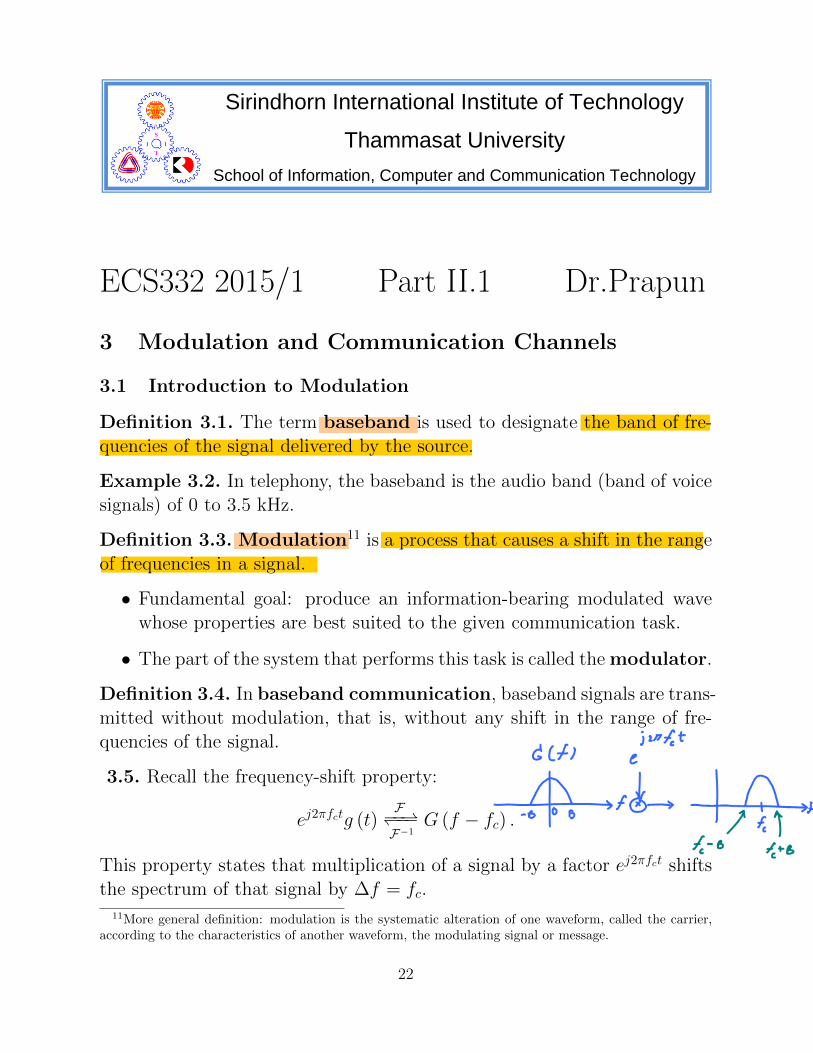
3 Modulation and Communication Channels

3.1 Introduction to Modulation

Definition 3.1. The term baseband is used to designate the band of fre-quencies of the signal delivered by the source.

Example 3.2. In telephony, the baseband is the audio band (band of voicesignals) of 0 to 3.5 kHz.

Definition 3.3. Modulation11 is a process that causes a shift in the rangeof frequencies in a signal.

• Fundamental goal: produce an information-bearing modulated wavewhose properties are best suited to the given communication task.

• The part of the system that performs this task is called the modulator.

Definition 3.4. In baseband communication, baseband signals are trans-mitted without modulation, that is, without any shift in the range of fre-quencies of the signal.

3.5. Recall the frequency-shift property:

ej2πfctg (t)F−−−−F−1

G (f − fc) .

This property states that multiplication of a signal by a factor ej2πfct shiftsthe spectrum of that signal by ∆f = fc.

11More general definition: modulation is the systematic alteration of one waveform, called the carrier,according to the characteristics of another waveform, the modulating signal or message.

22

3.6. Frequency-shifting (frequency translation) is easily achieved by “mul-tiplying” g(t) by a sinusoid:

g(t) cos(2πfct)F−−−−F−1

1

2(G(f − fc) +G(f + fc)) . (28)

0 5 10 15 20 25 30−4

−2

0

2

4

0 5 10 15 20 25 30−4

−2

0

2

4

0 5 10 15 20 25 30−4

−2

0

2

4

3.7. Similarly,

g(t) cos(2πfct+ φ)F−−−−F−1

1

2

(G(f − fc)ejφ +G(f + fc)e

−jφ) . (29)

23

Example 3.8. Plot (by hand) the Fourier transforms of the following sig-nals:

(a) cos(20πt)

(b) (cos(20πt))2

(c) cos(20πt)× cos(40πt)

(d) (cos(20πt))2 × cos(40πt)

Definition 3.9. The sinusoidal signals cos(2πfct) in (28) and cos(2πfct+φ)in (29) are called the (sinusoidal) carrier signals and fc is called the carrierfrequency. In general, it can also has amplitude A and hence the generalexpression of the carrier signal is A cos(2πfct+ φ).

Definition 3.10. Communication that uses modulation to shift the fre-quency spectrum of a signal is known as carrier communication. [4, p151]

Definition 3.11. We will use m(t) to denote the baseband signal. We willassume that m(t) is band-limited to B; that is, |M(f)| = 0 for |f | > B.Note that we usually call it the message or the modulating signal.

24

Example 3.12. A (Theoretically) Simple Modulator: Consider a messagem(t) produced by a source. Let the transmitted signal be

x(t) =√

2 cos (2πfct)×m(t).

Then,

X(f) =

√2

2M (f − fc) +

√2

2M (f + fc) .

The block diagram for this modulator is shown in Figure 4 which also in-cludes an example of the amplitude spectrum |M(f)| for the message m(t).With the given message spectrum and the carrier frequency being fc, theamplitude spectrum |X(f)| for the transmitted signal x(t) is also shown.

1

×

2 cos 2 cf t

Modulator

Message(modulating signal)

Figure 4: A simple modulator along with the amplitude spectrum plots of the signals.

Example 3.13. In Figure 5, an audio signal is used as the message m(t).

1 1.0005 1.001 1.0015 1.002 1.0025 1.003 1.0035 1.004 1.0045 1.005-1

-0.5

0

0.5

1

Seconds

-2.5 -2 -1.5 -1 -0.5 0 0.5 1 1.5 2 2.5

x 104

0

0.05

0.1

0.15

0.2

Frequency [Hz]

Mag

nitu

de

1 1.0005 1.001 1.0015 1.002 1.0025 1.003 1.0035 1.004 1.0045 1.005-1

-0.5

0

0.5

1

Seconds

-2.5 -2 -1.5 -1 -0.5 0 0.5 1 1.5 2 2.5

x 104

0

0.05

0.1

0.15

0.2

Frequency [Hz]

Mag

nitu

de

0 5 10 15 20 25-1

-0.5

0

0.5

1

Seconds

-2.5 -2 -1.5 -1 -0.5 0 0.5 1 1.5 2 2.5

x 104

0

0.05

0.1

0.15

0.2

Frequency [Hz]

Mag

nitu

de

0 5 10 15 20 25-2

-1

0

1

2

Seconds

-2.5 -2 -1.5 -1 -0.5 0 0.5 1 1.5 2 2.5

x 104

0

0.05

0.1

0.15

0.2

Frequency [Hz]

Mag

nitu

de/ 2

Figure 5: Signals in a simple modulator when an audio signal is used as its message.

25

Definition 3.14. The process of recovering the signal from the modulatedsignal (retranslating the spectrum to its original position) is referred to asdemodulation, or detection.

3.15. Modulation (spectrum shifting) benefits and applications:

(a) Reasonable antenna size:

• For effective radiation of power over a radio link, the antenna sizemust be on the order of the wavelength12 of the signal to be radi-ated.

• “Too low frequency” = “too large antenna”

• Audio signal frequencies are so low (wavelengths are so large) thatimpracticably large antennas will be required for radiation.

Shifting the spectrum to a higher frequency (a smaller wave-length) by modulation solves the problem.

(b) Frequency Assignment, Frequency-Division Multiplexing (FDM)and Frequency-Division Multiple Access (FDMA):

• If several signals (for example, all radio stations), each occupyingthe same frequency band, are transmitted simultaneously over thesame transmission medium, they will all interfere.

Difficult to separate or retrieve them at a receiver.

One solution is to use modulation whereby each radio stationis assigned a distinct carrier frequency.

12Efficient line-of-sight ratio propagation requires antennas whose physical dimensions are at least 1/10of the signal’s wavelength. [C&C [3], p. 8]

26

∗ Each station transmits a modulated signal, thus shifting thesignal spectrum to its allocated band, which is not occupiedby any other station.

∗ When you tune a radio or television set to a particular sta-tion, you are selecting one of the many signals being receivedat that time.

∗ Since each station has a different assigned carrier frequency,the desired signal can be separated from the others by fil-tering.

• Multiplexing is the process of combining (at the local level) sev-eral signals for simultaneous transmission on a common communi-cations resource.

• Multiple access (MA) involves remote sharing of the resource.

(c) Channel passband matching.

3.2 Communication Channel: Signal Distortion in Transmission

3.16. Recall that, for a linear, time-invariant (LTI) system, the input-output relationship is given by

y(t) = h(t) ∗ x(t)

where x(t) is the input, y(t) is the output, and h(t) is the impulse responseof the system.

27

In which case,Y (f) = H(f)X(f)

where H(f) is called the transfer function or frequency response ofthe system. |H(f)| and ∠H(f) are called the amplitude response (orgain) and phase response, respectively. Their plots as functions of f showat a glance how the system modifies the amplitudes and phases of varioussinusoidal inputs.

Example 3.17. An “extremely nice” channel that does nothing to its input:

y(t) = x(t).

Definition 3.18. A channel is called distortionless if

y(t) = βx(t− τ),

where β and τ are constants.

• The channel output has the same “shape” as its input.

• This is the “best” channel we can hope for. Any transmitted signalx(t) will need to travel over some distance before it reaches the re-ceiver. It will be delayed by the propagation time and its power willbe attenuated.

28

• A channel is distortionless if and only if it satisfies two properties:

(a) “flat” frequency response: constant amplitude response

(b) linear phase shift

3.19. Major types of distortion

(a) Linear distortion

(i) Amplitude distortion (frequency distortion): H(f) is not constantwith frequency.

(ii) Phase distortion (delay distortion): the phase shift is not linear;the various frequency components suffer different amounts of timedelay

(b) Nonlinear distortion: occur when the system includes nonlinear ele-ments

Example 3.20. Amplitude distortion (frequency distortion)

(a) Figure 6 shows signals in a channel with low-frequency attenuation

1

-10 -5 0 5 10-1.5

-1

-0.5

0

0.5

1

1.5

-10 -5 0 5 10-1.5

-1

-0.5

0

0.5

1

1.5

cos13 cos 3

15 cos 5 cos

13 cos 3

15 cos 5

-10 -5 0 5 10-1.5

-1

-0.5

0

0.5

1

1.5

-10 -5 0 5 10-1.5

-1

-0.5

0

0.5

1

1.5

Figure 6: Channel with low-frequency attenuation

29

1

-10 -5 0 5 10-1.5

-1

-0.5

0

0.5

1

1.5

-10 -5 0 5 10-1.5

-1

-0.5

0

0.5

1

1.5

cos13 cos 3

15 cos 5 cos

13 cos 3

15 cos 5

-10 -5 0 5 10-1.5

-1

-0.5

0

0.5

1

1.5

-10 -5 0 5 10-1.5

-1

-0.5

0

0.5

1

1.5

Figure 7: Channel with high-frequency attenuation

(b) Figure 7 shows signals in a channel with high-frequency attenuation

Example 3.21. A common area of confusion is constant time delayversus constant phase shift. The former is desirable and is required fordistortionless transmission. The latter, in general, causes distortion.

(a) Figure 8 shows signals in a channel with constant phase shift

1

-10 -5 0 5 10-1.5

-1

-0.5

0

0.5

1

1.5

-10 -5 0 5 10-1.5

-1

-0.5

0

0.5

1

1.5

cos13 cos 3

15 cos 5

-10 -5 0 5 10-1.5

-1

-0.5

0

0.5

1

1.5

-10 -5 0 5 10-1.5

-1

-0.5

0

0.5

1

1.5

cos2

13 cos 3

2

15 cos 5

2

Figure 8: Channel with constant phase shift

• Note that the peaks of the phase-shifted signal are substantiallygreater (by about 50 percent13) than those of the input test signal.

This is because the components of the distorted signal all attainmaximum or minimum values at the same time, which was nottrue of the input.

• Frequency response:

13Delay distortion is crucial in pulse transmission.On the other hand, an untrained human ear is insen-sitive to delay distortion. Thus, delay distortion is seldom of concern in voice and music transmission.

30

(b) Figure 9 shows signals in a channel with linear phase shift

1

-10 -5 0 5 10-1.5

-1

-0.5

0

0.5

1

1.5

-10 -5 0 5 10-1.5

-1

-0.5

0

0.5

1

1.5

cos13 cos 3

15 cos 5 cos

2

13 cos 3 3

2

15 cos 5 5

2

-10 -5 0 5 10-1.5

-1

-0.5

0

0.5

1

1.5

-10 -5 0 5 10-1.5

-1

-0.5

0

0.5

1

1.5

Figure 9: Channel with linear phase shift

Note that

y (t) = cos(t+

π

2

)− 1

3cos(

3t+ 3π

2

)+

1

5cos(

5t+ 5π

2

)= cos

(t+

π

2

)− 1

3cos(

3(t+

π

2

))+

1

5cos(

5(t+

π

2

))= x

(t+

π

2

)Therefore, this linear phase shift is the same as the time-shift opera-

tion.

3.22. Multipath Propagation and Time Dispersion [6, p 1]

• In wireless channel, the presence of multiple scatterers (buildings, ve-hicles, hills, and so on) causes the transmitted radio wave to propa-gate along several different paths (rays) that terminate at the receiver.Hence, the receive antenna picks up a superposition of multiple atten-uated and delayed copies of the transmitted signal.

This phenomenon is referred to as multipath propagation. [6, p 1]

• Due to different lengths of the propagation paths, the individual mul-tipath components experience different delays (time shifts) [6, p 1]:

y (t) = x (t) ∗ h (t) =v∑i=0

βix (t− τi)

where

h (t) =v∑i=0

βiδ (t− τi).

31

Figure 10: Multipath Propagation

Here, βi = |βi|ejφi and τi are, respectively, the complex attenuationfactor and delay associated with the ith path.

• The receiver observes a temporally smeared-out version of the transmitsignal. Such channels are termed time-dispersive

• The corresponding frequency response of the channel is

H (f) =v∑i=0

βie−j2πfτi. (30)

• Time-dispersive channels are frequency-selective in the sense thatdifferent frequencies are attenuated differently. This is clear from thef -dependent H(f) in (30).

These differences in attenuation become more severe when the dif-ference of the path delays is large and the difference between thepath attenuations is small. [6, p 3]

∗ This can be seen from the expression in Ex. 3.23.

• Although multipath propagation has traditionally been viewed as atransmission impairment, nowadays there is a tendency to consider it asbeneficial since it provides additional degrees of freedom that are knownas delay diversity or frequency diversity and that can be exploited torealize diversity gains or, in the context of multiantenna systems, evenmultiplexing gains. [6]

32

Example 3.23. Two-path channel: Consider two propagation paths ina static environment. The receive signal is given by

y(t) = β1x(t− τ1) + β2x(t− τ2).

In which case,h(t) = β1δ(t− τ1) + β2δ(t− τ2)

and

H(f) = β1e−j2πfτ1 + β2e

−j2πfτ2 = |β1| ejφ1e−j2πfτ1 + |β2| ejφ2e−j2πfτ2.

Recall that |Z1 + Z2|2 = |Z1|2 + |Z2|2 + 2Re Z1Z∗2. Therefore,

|H (f)|2 = |β1|2 + |β2|2 + 2 Re|β1| ejφ1e−j2πfτ1

(|β2| ejφ2e−j2πfτ2

)∗

= |β1|2 + |β2|2 + 2 |β1| |β2| cos (2π (τ2 − τ1) f + (φ1 − φ2)) .

33

Example 3.24. Consider the two-path channels in which the receive signalis given by

y(t) = β1x(t− τ1) + β2x(t−]τ2).

Four different cases are considered.

(a) Small |τ1 − τ2| and |β1| |β2|

(b) Large |τ1 − τ2| and |β1| |β2|

(c) Small |τ1 − τ2| and |β1| ≈ |β2|

(d) Large |τ1 − τ2| and |β1| ≈ |β2|

-1.5 -1 -0.5 0 0.5 1 1.5-30

-20

-10

0

f

[dB

]

(i)

-1.5 -1 -0.5 0 0.5 1 1.5-30

-20

-10

0

f

[dB

]

(ii)

-1.5 -1 -0.5 0 0.5 1 1.5-30

-20

-10

0

f

[dB

]

(iii)

-1.5 -1 -0.5 0 0.5 1 1.5-30

-20

-10

0

f

[dB

]

(iv)

Figure 11: Frequency selectivity in the receive spectra (blue line) for two-path channels.

Figure 11 shows four plots of normalized14 |X(f)| (dotted black line15)and normalized |Y (f)| (solid blue line) in [dB]. Match the four graphs (i-iv)to the four cases (a-d).

14The function is normalized so that the maximum point is 0 dB.15For those who are curious, x(t) is a raised cosine pulse with roll-off factor α = 0.2 and symbol duration

T = 0.5.

34

4 Amplitude/Linear Modulation

4.1. A sinusoidal carrier signal A cos(2πfct+φ) has three basic parameters:amplitude, frequency, and phase. Varying these parameters in proportionto the baseband signal results in amplitude modulation (AM), frequency16

modulation (FM), and phase modulation (PM), respectively. Collectively,these techniques are called continuous-wave (CW) modulation [13, p111][3, p 162].

Definition 4.2. Amplitude modulation is characterized by the fact thatthe amplitude A of the carrier A cos(2πfct + φ) is varied in proportion tothe baseband (message) signal m(t).

• Because the amplitude is time-varying, we may write the modulatedcarrier as

A(t) cos(2πfct+ φ)

• Because the amplitude is linearly related to the message signal, thistechnique is also called linear modulation.

4.3. Linear modulations:

(a) Double-sideband amplitude modulation

(i) Double-sideband-suppressed-carrier (DSB-SC or DSSC or simplyDSB) modulation

(ii) Standard amplitude modulation (AM)

(b) Suppressed-sideband amplitude modulation

(i) Single-sideband modulation (SSB)

(ii) Vestigial-sideband modulation (VSB)

16Technically, the variation of “frequency” is not as straightforward as the description here seems tosuggest. For a sinusoidal carrier, a general modulated carrier can be represented mathematically as

x(t) = A(t) cos (2πfct+ φ(t)) .

Frequency modulation, as we shall see later, is resulted from letting the time derivative of φ(t) be linearlyrelated to the modulating signal. [14, p 112]

35

4.1 Double-sideband suppressed carrier (DSB-SC) modulation

Definition 4.4. In double-sideband-suppressed-carrier (DSB-SC orDSSC or simply DSB) modulation, the modulated signal is

x(t) = Ac cos (2πfct)×m(t).

We have seen that the multiplication by a sinusoid gives two shifted andscaled replicas of the original signal spectrum:

X(f) =Ac

2M (f − fc) +

Ac

2M (f + fc) .

• When we set Ac =√

2, we get the “simple” modulator discussed inExample 3.12.

• We need fc > B to avoid spectral overlapping. In practice, fc B.

4.5. Synchronous/coherent detection by the product demodulator:The incoming modulated signal is first multiplied with a locally generatedsinusoid with the same phase and frequency (from a local oscillator (LO))and then lowpass-filtered, the filter bandwidth being the same as the mes-sage bandwidth B or somewhat larger.

4.6. A DSB-SC modem with no channel impairment is shown in Figure 12.

× ×Channel

2 cos 2 cf t

y

2 cos 2 cf t

vLPF

Modulator Demodulator

Message(modulating signal)

22

Figure 12: DSB-SC modem with no channel impairment

36

Once again, recall that

X (f) =√

2

(1

2(M (f − fc) +M (f + fc))

)=

1√2

(M (f − fc) +M (f + fc)) .

Similarly,

v (t) = y (t)×√

2 cos (2πfct) =√

2x (t) cos (2πfct)

V (f) =1√2

(X (f − fc) +X (f + fc))

Alternatively, we can work in the time domain and utilize the trig. iden-tity from Example 2.4:

v (t) =√

2x (t) cos (2πfct) =√

2(√

2m (t) cos (2πfct))

cos (2πfct)

= 2m (t) cos2 (2πfct) = m (t) (cos (2 (2πfct)) + 1)

= m (t) +m (t) cos (2π (2fc) t)

Key equation for DSB-SC modem:

LPF

(m (t)×

√2 cos (2πfct)

)︸ ︷︷ ︸

x(t)

×(√

2 cos (2πfct)) = m (t) . (31)

37

4.7. Implementation issues:

(a) Problem 1: Modulator construction

(b) Problem 2: Synchronization between the two (local) carriers/oscillators

(c) Problem 3: Spectral inefficiency

4.8. Spectral inefficiency/redundancy: When m(t) is real-valued, itsspectrum M(f) has conjugate symmetry. With such message, the corre-sponding modulated signal’s spectrum X(f) will also inherit the symmetrybut now centered at fc (instead of at 0). The portion that lies above fc isknown as the upper sideband (USB) and the portion that lies below fcis known as the lower sideband (LSB). Similarly, the spectrum centeredat −fc has upper and lower sidebands. Hence, this is a modulation schemewith double sidebands. Both sidebands contain the same (and complete)information about the message.

4.9. Synchronization: Observe that (31) requires that we can generatecos (ωct) both at the transmitter and receiver. This can be difficult in prac-tice. Suppose that the frequency at the receiver is off, say by ∆f , and thatthe phase is off by θ. The effect of these frequency and phase offsets can bequantified by calculating

LPF(m (t)

√2 cos (2πfct)

)√2 cos (2π (fc + ∆f) t+ θ)

,

which givesm (t) cos (2π (∆f) t+ θ) .

Of course, we want ∆ω = 0 and θ = 0; that is the receiver must generatea carrier in phase and frequency synchronism with the incoming carrier.

38

4.10. Effect of time delay:

Suppose the propagation time is τ , then we have

y (t) = x (t− τ) =√

2m (t− τ) cos (2πfc (t− τ))

=√

2m (t− τ) cos (2πfct− 2πfcτ)

=√

2m (t− τ) cos (2πfct− φτ) .

Consequently,

v (t) = y (t)×√

2 cos (2πfct)

=√

2m (t− τ) cos (2πfct− φτ)×√

2 cos (2πfct)

= m (t− τ) 2 cos (2πfct− φτ) cos (2πfct) .

Applying the product-to-sum formula, we then have

v (t) = m (t− τ) (cos (2π (2fc) t− φτ) + cos (φτ)) .

In conclusion, we have seen that the principle of the DSB-SC modem isbased on a simple key equation (31). However, as mentioned in 4.7, thereare several implementation issues that we need to address. Some solutionsare provided in the subsections to follow. However, the analysis will requiresome knowledge of Fourier series which is reviewed in the next subsection.

39

4.2 Fourier Series

Definition 4.11. Exponential Fourier series: Let the (real or complex)signal r (t) be a periodic signal with period T0. Suppose the following Dirich-let conditions are satisfied

(a) r (t) is absolutely integrable over its period; i.e.,T0∫0

|r (t)|dt <∞.

(b) The number of maxima and minima of r (t) in each period is finite.

(c) The number of discontinuities of r (t) in each period is finite.

Then r (t) can be expanded in terms of the complex exponential signals(ejnω0t

)∞n=−∞ as

r (t) =∞∑

n=−∞cne

jnω0t = c0 +∞∑k=1

(cke

jkω0t + c−ke−jkω0t

)(32)

where

ω0 = 2πf0 =2π

T0,

ck =1

T0

α+T0∫

α

r (t) e−jkω0tdt, (33)

for some arbitrary α. In which case,

r (t) =

r (t) , if r (t) is continuous at tr(t+)+r(t−)

2 , if r (t) is not continuous at t

We give some remarks here.

• The parameter α in the limits of the integration (33) is arbitrary. Itcan be chosen to simplify computation of the integral. Some references

40

simply write ck = 1T0

∫T0

r (t) e−jkω0tdt to emphasize that we only need

to integrate over one period of the signal; the starting point is notimportant.

• The coefficients ck = 1T0

∫T0

r (t) e−jkω0tdt are called the (kth) Fourier

(series) coefficients of (the signal) r (t). These are, in general, com-plex numbers.

• c0 = 1T0

∫T0

r (t) dt = average or DC value of r(t)

• The quantity f0 = 1T0

is called the fundamental frequency of thesignal r (t). The nth multiple of the fundamental frequency (for positiven’s) is called the nth harmonic.

• ckejkω0t + c−ke−jkω0t = the kth harmonic component of r (t).

k = 1 ⇒ fundamental component of r (t).

4.12. Getting the Fourier coefficients from the Fourier transform:Consider a restricted version rT0(t) of r(t) where we only consider r(t) for

one specific period. Suppose rT0(t)F−−−−F−1

RT0(f). Then,

ck =1

T0RT0(kf0).

So, the Fourier coefficients are simply scaled samples of the Fouriertransform.

Example 4.13. Find the Fourier series expansion for the train of impulses

δ(T0)(t) =∞∑

n=−∞δ (t− nT0) drawn in Figure 13.

0T 02T t

Figure 13: Train of impulses

41

4.14. The Fourier series in Example 4.13 gives an interesting Fourier trans-form pair:

A special case when T0 = 1 is quite easy to remember:

We can use the scaling property of the delta function to generalize the specialcase:

Example 4.15. Find the Fourier coefficients of the square pulse periodicsignal [5, p 57]shown in Figure 14. Note that multiplication by this signalis equivalent to a switching (ON-OFF) operation.

1

T0

4T0

4T0 2T0T02T0

1

t

Figure 14: Square pulse periodic signal

4.16. Parseval’s Identity: Pr = 1T0

∫T0

|r (t)|2 dt =∞∑

k=−∞|ck|2

42

4.17. Fourier series expansion for real valued function: Supposer (t) in the previous section is real-valued; that is r∗ = r. Then, we havec−k = c∗k and we provide here three alternative ways to represent the Fourierseries expansion:

r (t) =∞∑

n=−∞cne

jnω0t = c0 +∞∑k=1

(cke

jkω0t + c−ke−jkω0t

)(34)

= c0 +∞∑k=1

(ak cos (kω0t)) +∞∑k=1

(bk sin (kω0t)) (35)

= c0 + 2∞∑k=1

|ck| cos (kω0t+ ∠ck) (36)

where the corresponding coefficients are obtained from

ck =1

T0

α+T0∫

α

r (t) e−jkω0tdt =1

2(ak − jbk) (37)

ak = 2Re ck =2

T0

∫T0

r (t) cos (kω0t) dt (38)

bk = −2Im ck =2

T0

∫T0

r (t) sin (kω0t) dt (39)

2 |ck| =√a2k + b2

k (40)

∠ck = − arctan

(bkak

)(41)

c0 =a0

2(42)

The Parseval’s identity can then be expressed as

Pr =1

T0

∫T0

|r (t)|2 dt =∞∑

k=−∞

|ck|2 = c20 + 2

∞∑k=1

|ck|2

43

4.18. To go from (34) to (35) and (36), note that when we replace c−k byc∗k, we have

ckejkω0t + c−ke

−jkω0t = ckejkω0t + c∗ke

−jkω0t

= ckejkω0t +

(cke

jkω0t)∗

= 2 Recke

jkω0t.

• Expression (36) then follows directly from the phasor concept:

Recke

jkω0t

= |ck| cos (kω0t+ ∠ck) .

• To get (35), substitute ck by Re ck+ j Im ckand ejkω0t by cos (kω0t) + j sin (kω0t).

Example 4.19. For the train of impulses in Example 4.13,

δ(T0)(t) =∞∑

k=−∞

δ (t− kT0) =1

T0

∞∑k=−∞

ejkω0t =1

T0+

2

T0

∞∑k=1

cos kω0t (43)

Example 4.20. For the rectangular pulse train in Example 4.15,

1 [cosω0t ≥ 0] =1

2+

2

π

(cosω0t−

1

3cos 3ω0t+

1

5cos 5ω0t−

1

7cos 7ω0t+ . . .

)(44)

Example 4.21. Bipolar square pulse periodic signal [5, p 59]:

sgn(cosω0t) =4

π

(cosω0t−

1

3cos 3ω0t+

1

5cos 5ω0t−

1

7cos 7ω0t+ . . .

)

1

-1

0T 0T− t

1

0T 0T− t

Figure 15: Bipolar square pulse periodic signal

44

4.3 Classical DSB-SC Modulators

To produce the modulated signal Ac cos(2πfct)m(t), we may use the follow-ing methods which generate the modulated signal along with other signalswhich can be eliminated by a bandpass filter restricting frequency contentsto around fc.

4.22. Multiplier Modulators [5, p 184] or Product Modulator[3, p180]: Here modulation is achieved directly by multiplying m(t) by cos(2πfct)using an analog multiplier whose output is proportional to the product oftwo input signals.

• Such a multiplier may be obtained from

(a) a variable-gain amplifier in which the gain parameter (such as thethe β of a transistor) is controlled by one of the signals, say, m(t).When the signal cos(2πfct) is applied at the input of this amplifier,the output is then proportional to m(t) cos(2πfct).

(b) two logarithmic and an antilogarithmic amplifiers with outputsproportional to the log and antilog of their inputs, respectively.

Key equation:A×B = e(lnA+lnB).

4.23. Square Modulator: When it is easier to build a squarer than amultiplier, use

(m (t) + c cos (ωct))2 = m2 (t) + 2cm (t) cos (ωct) + c2 cos2 (ωct)

= m2 (t) + 2cm (t) cos (ωct) +c2

2+c2

2cos (2ωct) .

45

• Alternative, can use(m(t) + c cos

(ωc2 t))3

.

4.24. Multiply m(t) by “any” periodic and even signal r(t) whose periodis Tc = 2π

ωc. Because r(t) is an even function, we know that

r (t) = c0 +∞∑k=1

ak cos (kωct) for some c0, a1, a2, . . ..

Therefore,

m(t)r (t) = c0m(t) +∞∑k=1

akm(t) cos (kωct).

See also [4, p 157]. In general, for this scheme to work, we need

( )M ω ( )m r ω×F

cω 2 cω cω− 2 cω−

0c A 112

Aa 2

12

Aa A

2 Bπ 2 Bπ 2c Bω π−

× ( )m t

( )r t

BPF ( ) ( )cos cm t tω

BPF

Figure 16: Modulation of m(t) via even and periodic r(t)

• a1 6= 0; that is Tc is the “least” period of r;

• fc > 2B (to prevent overlapping).

Note that if r(t) is not even, then by (36), the outputted modulatedsignal is of the form a1m(t) cos(ωct+ φ1).

46

4.25. Switching modulator : Set r(t) to be the square pulse train givenby (44):

r (t) = 1 [cosω0t ≥ 0]

=1

2+

2

π

(cosω0t−

1

3cos 3ω0t+

1

5cos 5ω0t−

1

7cos 7ω0t+ . . .

).

Multiplying this r(t) to the signal m(t) is equivalent to switching m(t) onand off periodically.

It is equivalent to periodically turning the switch on (letting m(t) passthrough) for half a period Tc = 1

fc.

186 AMPLITUDE MODULATIONS AND DEMODULATIONS

Figure 4.4 Switching modulator for DSB-SC.

m(t )

~

w(l)

nnnnnnnnnnnnn

(a)

(b)

0 I

J~

The square pulse train w(t) in Fig. 4.4b is a periodic signal whose Fourier series was found earlier in Example 2.8 [Eq. (2.86)] as

ll' (l) = ~ + ~ (cos We t - ~ cos 3wct + ~ cos Seve! - · · · ) 2 J[ .) )

(4 .S )

The signalm (t)lr (t) is given by

m (t)w(t) = -m(t) + - m (t) cos eve! - -m(!) cos 3wct + -::111 (1) cos Seve! - · · · l 2 [ I l ] 2 J[ 3 )

(4.6)

The signal m(l) ll '(t) consists not onl y of the component 111(1) bu t a lso of an infinite number of modulated signals with angul ar frequencies r»c, 3wc, Seve, .. .. Therefore, the spectrum of m(1)1-v(t) consists of multiple copies of the message spectrum M (f), shifted to 0, ±fc, ±~fc , ±Sf~- , .. . (with decreas ing re lat ive weights), as shown in Fig. 4.4c.

For modulation , we are interested in extracting the modulated component m.(t) cos We i

on ly. To separate this component from the rest of the crowd, we pass the signal m(t)w(t) through a bandpass filter of band width 28 Hz (or 4Tr8 rad/s) , centered at the frequency ±fc· Provided the carrier angular frequency.fc ::::: 28 (or We ::::: 4Tr8) , thi s will suppress all the spectral components not centered at ±fc to yield the des ired modulated signal (2/ Tr)m(t) cos We t (Fig. 4.4d).

We now see the real payoff of this method. Multipl ication of a signal by a square pulse train is in reality a switching operation. It involves switching the signal m(t) on and off periodically and can be accomplished by simple switching elements controlled by w(t). Figure 4 .Sa shows one such electronic switch, the diode bridge modulator, driven by a sinusoid A cos We t to produce the switching action. Diodes D 1, D2 and D3, D4 are matched pairs. When the signal cos Wet is of a polarity that wi ll make terminal c positive with respect to d, all the diodes

Figure 17: Switching modulator for DSB-SC [4, Figure 4.4].

4.26. Switching Demodulator :

LPFm(t) cos(ωct)× 1[cos(ωct) ≥ 0] =1

πm(t) (45)

[4, p 162]. Note that this technique still requires the switching to be in syncwith the incoming cosine as in the basic DSB-SC.

47

4.4 Energy and Power

Definition 4.27. For a signal g(t), the instantaneous power p(t) dissipatedin the 1-Ω resister is pg(t) = |g(t)|2 regardless of whether g(t) represents avoltage or a current. To emphasize the fact that this power is based uponunity resistance, it is often referred to as the normalized power.

Definition 4.28. The total (normalized) energy of a signal g(t) is givenby

Eg =

∫ +∞

−∞pg(t)dt =

∫ +∞

−∞|g(t)|2 dt = lim

T→∞

∫ T

−T|g(t)|2 dt.

4.29. By the Parseval’s theorem discussed in 2.39, we have

Eg =

∫ ∞−∞|g(t)|2dt =

∫ ∞−∞|G(f)|2df.

Definition 4.30. The average (normalized) power of a signal g(t) is givenby

Pg = limT→∞

1

T

T/2∫−T/2

|g (t)|2dt = limT→∞

1

2T

∫ T

−T|g(t)|2 dt.

Definition 4.31. To simplify the notation, there are two operators thatused angle brackets to define two frequently-used integrals:

(a) The “time-average” operator:

〈g〉 ≡ 〈g (t)〉 ≡ limT→∞

1

T

∫ T/2

−T/2g (t)dt = lim

T→∞

1

2T

∫ T

−Tg (t)dt (46)

(b) The inner-product operator:

〈g1, g2〉 ≡ 〈g1 (t) , g2 (t)〉 =

∫ ∞−∞

g1(t)g∗2(t)dt (47)

4.32. Using the above definition, we may write

• Eg = 〈g, g〉 = 〈G,G〉 where G = F g

• Pg =⟨|g|2⟩

48

• Parseval’s theorem: 〈g1, g2〉 = 〈G1, G2〉where G1 = F g1 and G2 = F g2

4.33. Time-Averaging over Periodic Signal: For periodic signal g(t) withperiod T0, the time-average operation in (46) can be simplified to

〈g〉 =1

T0

∫T0

g (t)dt

where the integration is performed over a period of g.

Example 4.34. 〈cos (2πf0t+ θ)〉 =

Similarly, 〈sin (2πf0t+ θ)〉 =

Example 4.35.⟨cos2 (2πf0t+ θ)

⟩=

Example 4.36.⟨ej(2πf0t+θ)

⟩= 〈cos (2πf0t+ θ) + j sin (2πf0t+ θ)〉

Example 4.37. Suppose g(t) = cej2πf0t for some (possibly complex-valued)constant c and (real-valued) frequency f0. Find Pg.

4.38. When the signal g(t) can be expressed in the form g(t) =∑k

ckej2πfkt

and the fk are distinct, then its (average) power can be calculated from

Pg =∑k

|ck|2

49

Example 4.39. Suppose g(t) = 2ej6πt + 3ej8πt. Find Pg.

Example 4.40. Suppose g(t) = 2ej6πt + 3ej6πt. Find Pg.

Example 4.41. Suppose g(t) = cos (2πf0t+ θ). Find Pg.Here, there are several ways to calculate Pg. We can simply use Ex-

ample 4.35. Alternatively, we can first decompose the cosine into complexexponential functions using the Euler’s formula:

4.42. The (average) power of a sinusoidal signal g(t) = A cos(2πf0t+ θ) is

Pg =

12 |A|

2, f0 6= 0,

|A|2cos2θ, f0 = 0.

This property means any sinusoid with nonzero frequency can be written inthe form

g (t) =√

2Pg cos (2πf0t+ θ) .

4.43. Extension of 4.42: Consider sinusoids Ak cos (2πfkt+ θk) whose fre-quencies are positive and distinct. The (average) power of their sum

g(t) =∑k

Ak cos (2πfkt+ θk)

is

Pg =1

2

∑k

|Ak|2.

50

Example 4.44. Suppose g (t) = 2 cos(2π√

3t)

+ 4 cos(2π√

5t). Find Pg.

4.45. For periodic signal g(t) with period T0, there is also no need to carryout the limiting operation to find its (average) power Pg. We only need tofind an average carried out over a single period:

Pg =1

T0

∫T0

|g (t)|2dt.

(a) When the corresponding Fourier series expansion g(t) =∞∑

n=−∞cne

jnω0t

is known,

Pg =∞∑

k=−∞

|ck|2

(b) When the signal g(t) is real-valued and its (compact) trigonometric

Fourier series expansion g(t) = c0 + 2∞∑k=1

|ck| cos (kω0t+ ∠ck) is known,

Pg = c20 + 2

∞∑k=1

|ck|2

Definition 4.46. Based on Definitions 4.28 and 4.30, we can define threedistinct classes of signals:

(a) If Eg is finite and nonzero, g is referred to as an energy signal.

(b) If Pg is finite and nonzero, g is referred to as a power signal.

(c) Some signals17 are neither energy nor power signals.

• Note that the power signal has infinite energy and an energy signal haszero average power; thus the two categories are mutually exclusive.

Example 4.47. Rectangular pulse

17Consider g(t) = t−1/41[t0,∞)(t), with t0 > 0.

51

Example 4.48. Sinc pulse

Example 4.49. For α > 0, g(t) = Ae−αt1[0,∞)(t) is an energy signal withEg = |A|2/2α.

Example 4.50. The rotating phasor signal g(t) = Aej(2πf0t+θ) is a powersignal with Pg = |A|2.Example 4.51. The sinusoidal signal g(t) = A cos(2πf0t + θ) is a powersignal with Pg = |A|2/2.

4.52. Consider the transmitted signal

x(t) = m(t) cos(2πfct+ θ)

in DSB-SC modulation. Suppose M(f − fc) and M(f + fc) do not overlap(in the frequency domain).

(a) If m(t) is a power signal with power Pm, then the average transmittedpower is

Px =1

2Pm.

(b) If m(t) is an energy signal with energy Em, then the transmitted energyis

Ex =1

2Em.

• Q: Why is the power (or energy) reduced?

• Remark: When x(t) =√

2m(t) cos(2πfct + θ) (with no overlappingbetween M(f − fc) and M(f + fc)), we have Px = Pm.

52