Ecosystem and Environmental Indicators for Deepwater Fisheries
149
Ecosystem and Environmental Indicators for Deepwater Fisheries New Zealand Aquatic Environment and Biodiversity Report No. 127 I.D. Tuck M.H. Pinkerton D.M. Tracey O.A. Anderson S.M. Chiswell ISSN 1179-6480 (online) ISBN 978-0-478-42399-0 (online) April 2014
Transcript of Ecosystem and Environmental Indicators for Deepwater Fisheries

Ecosystem and Environmental Indicators for Deepwater Fisheries
New Zealand Aquatic Environment and Biodiversity Report No. 127 I.D. Tuck
M.H. Pinkerton D.M. Tracey O.A. Anderson S.M. Chiswell
ISSN 1179-6480 (online) ISBN 978-0-478-42399-0 (online)
April 2014
Requests for further copies should be directed to: Publications Logistics Officer Ministry for Primary Industries PO Box 2526 WELLINGTON 6140 Email: [email protected] Telephone: 0800 00 83 33 Facsimile: 04-894 0300 This publication is also available on the Ministry for Primary Industries websites at: http://www.mpi.govt.nz/news-resources/publications.aspx http://fs.fish.govt.nz go to Document library/Research reports © Crown Copyright - Ministry for Primary Industries

TABLE OF CONTENTS
1 INTRODUCTION 3
2 PURPOSE, CHARACTERISTICS AND FRAMEWORKS FOR INDICATORS 6 2.1 Purpose 6
2.1.1 Process studies 6 2.1.2 Regime shift 6 2.1.3 Headline indicators 7 2.1.4 Indicators for ecosystem erosion 7 2.1.5 Climate/oceanographic vs fishery-induced change 8
2.2 Criteria for evaluating indicators 10
2.2.1 Indicator reference points, envelopes and directions 11 2.3 DPSIR framework 11
2.4 Indicators grouped by topic area 13
3 CLIMATE INDICES 14 3.1 Interdecadal Pacific Oscillation (IPO) 15
3.2 Southern Oscillation Index (SOI) 16
3.3 Antarctic Oscillation 17
3.4 Kidson weather types 19
3.5 Ocean winds 19
3.6 Recommended candidate Climate indicators 20
4 OCEANOGRAPHIC INDICES 20 4.1 Ocean temperature 21
4.1.1 Impacts of temperature change on ocean communities 21 4.1.2 Satellite observation of sea surface temperature 21 4.1.3 Bulk water temperature 22 4.1.4 Sea-bed temperature 23
4.2 Ocean circulation 24
4.2.1 Sea Surface Height from Satellite 26 4.2.2 Current measurements: Current meters 26 4.2.3 Current measurements: Shipboard ADCP 27 4.2.4 Current measurements: Global Drifters 27
4.3 Ocean Acidity 28
4.4 Hypoxia / Anoxia 31
4.5 Recommended candidate Oceanographic indicators 31
5 PRIMARY PRODUCTIVITY 32 5.1 Phytoplankton biomass 32
5.1.1 Satellite measurements of ocean colour 32 5.1.2 Ocean colour satellite sensors 32

5.1.3 Satellite ocean colour algorithms 33 5.1.4 Patterns in climatological chlorophyll-a 34 5.1.5 Carbon-chlorophyll ratios for marine phytoplankton 38
5.2 Primary productivity 38
5.2.1 Satellite-based methods of measuring NPP 39 5.2.2 NPP estimates for the New Zealand region 40 5.2.3 Effects of climate change on primary productivity 44
5.3 Variation from baseline 45
5.4 Recommended candidate indicators for Primary productivity 45
6 FOOD-WEB INDICATORS 46 6.1 Trophic ecosystem services supporting fisheries 46
6.2 Prey species for commercially-important fish 47
6.3 Bentho-pelagic coupling 48
6.4 Indicators for middle trophic level organisms 49
6.5 Recommended candidate indicators for Food webs 50
7 FISHERIES AND FISHERIES MANAGEMENT INDICATORS 51 7.1 Fishing pressure indicators 51
7.1.1 Fishing removals 51 7.1.2 Fishing effort 51
7.2 Fisheries Management Response Indicators 53
7.2.1 State of fisheries knowledge 53 7.2.2 Bioregions protected indicator 53 7.2.3 Fisheries management indicators 55
7.3 Recommended candidate indicators for Fisheries and Fisheries management 56
8 DEEPWATER FISH COMMUNITY INDICATORS 56 8.1 Exploited fish (targeted species) 57
8.2 Diversity 59
8.3 Community composition 61
8.4 Size composition 63
8.5 Trophodynamic (food-web) indicators 65
8.6 Recommended candidate indicators for Deepwater fish communities 67
9 BENTHIC COMMUNITIES AND HABITATS (SEA-FLOOR INTEGRITY) 68 9.1 Substrate characteristics 68
9.2 Benthic communities 69
9.2.1 Deepwater hard corals 69 9.3 Recommended candidate indicators for Benthic communities and habitats 70
10 TOP PREDATORS & THREATENED/PROTECTED SPECIES 71 10.1 Top predators 71
10.2 Threatened/protected species 71
10.3 Candidate indicators 72

10.4 Recommended candidate indicators for Top predators and Threatened/Protected species 73
11 ROLE OF OBSERVERS 74 11.1 Overview 74
11.2 The New Zealand Government Fisheries Observer Programme 74
11.3 Review of existing data and procedures 75
11.3.1 Observer key roles 75 11.3.2 Observer vessel placement and coverage 76 11.3.3 At-sea data recording 77 11.3.4 Use of observer data 79
11.4 Identification tools and data accuracy 80
12 CONCLUSIONS 82 12.1 General conclusions 82
12.2 Climate, oceanographic, environmental indicators 82
12.3 Food-web indicators 83
12.4 Fisheries and fisheries management indicators 84
12.5 Indicators of the deepwater fish community 84
12.6 Benthic communities and habitats 85
12.7 Top predators and threatened/protected species 85
13 RECOMMENDATIONS 86 13.1 Additional research recommended for indicators 90
13.2 Additional and /or modifications to existing data collection recommended for indicators 91
14 ACKNOWLEDGMENTS 99
15 REFERENCES 99
16 APPENDICES 132 16.1 Deepwater fisheries and stocks as defined by MPI 132
16.2 Observer coverage in Deepwater fisheries 133
16.3 Spatial distribution of observed fishing events 134
16.4 Observed fishing events by method and fishing year for deepwater fisheries 136
16.5 Observer forms 137
16.6 Databases relevant to observer programme deepwater fisheries data collection 142


Ministry for Primary Industries Ecosystem and environmental indicators for deepwater fisheries • 1
EXECUTIVE SUMMARY Tuck, I.D.; Pinkerton, M.H.; Tracey, D.M.; Anderson, O.A.; Chiswell, S.M. (2014). Ecosystem and environmental indicators for deepwater fisheries. New Zealand Aquatic Environment and Biodiversity Report No. 127. 143 p.
• This report provides a review of fisheries and environmental indicators and methods that could be used to monitor and analyse environmental and ecosystem changes. The recommended list is in no order of priority, and is intended to help the Ministry for Primary Industries in assessing the performance of deepwater fisheries and environments (deeper than 200 m).
• There are a number of different purposes of developing ecosystem indicators related
to fisheries management. These include relating trends in climate, environmental or oceanic conditions to productivity of a species or stock (e.g. year class strength) for use in single-species management; early-warning systems for regime shift; headline indicators for monitoring, communicating and comparing overall change in ecosystems; indicators to monitor for long-term ecosystem erosion or reduced resilience; adding climate/oceanographic context to observed fisheries variability and change. The best set of indicators will be different for different purposes, so that clarity in defining the purpose of indicators is likely to lead to better outcomes.
• Previous reviews have concluded that no single indicator addresses all aspects of an
ecosystem, and that a suite of indicators are required to monitor and summarise change in ecosystems. Such a suite of indicators should be sensitive to change across the range of scales and processes. We have examined and identified indicators across the following eight categories: (1) climate; (2) oceanographic; (3) primary productivity; (4) food-web; (5) fisheries and fisheries management; (6) the fish community; (7) benthic communities and habitats (sea-floor integrity); and (8) top predators, threatened and endangered species.
• A number of indices of variation in the regional climate system exist describing
variation over different time scales (e.g. Southern Oscillation Index, Interdecadal Pacific Oscillation and the Antarctic Oscillation). Spatio-temporal analysis of the over twenty year archive of oceanographic satellite data of the New Zealand region is recommended to identify trends and variability that may be of relevance to fisheries. Ongoing analysis of this type may act as an early warning for climate-driven regime shift in the New Zealand region.
• In the New Zealand region oceanographic state and variability are likely to become
increasingly important drivers of marine ecosystems as global climate change continues. Studies show that climate, oceanographic and environmental drivers can impact ecosystems at least as strongly as fishing, and as well can act synergistically with fishing to cause long-term change in marine ecosystems which can affect sustainable long-term fisheries yield.
• Indicators of key prey species of commercially-important fish should be sought. The key groups to track are mesopelagic fishes (particularly myctophids), crustacean

2 • Ecosystem and environmental indicators for deepwater fisheries Ministry for Primary Industries
macrozooplankton (particularly krill), gelatinous zooplankton (particularly salps and siphonophores) and mesozooplankton. Surveys involving the use of multifrequency acoustics and the Continuous Plankton Recorder (CPR) are recommended to estimate biomass and community composition.
• Suggested indicators of fishing removals, fishing effort (particularly in relation to
benthic disturbance), and management activity/response are given. The data required for these indicators are generally collected routinely at present.
• Standardised trawl survey information should be used to develop indicators of
changes in the deepwater fish community of the Chatham Rise and sub-Antarctic regions. Recommended indicators include trends in target species and total community biomass, biomass ratios (e.g., piscivore–planktivore or pelagic–demersal), measures of community diversity, the proportion of large fish and mean trophic level.
• Benthic communities and habitats provide valuable ecosystem functions, through linking benthic and pelagic systems, and also providing habitat structure, but can be vulnerable to disturbance from mobile fishing gear. Recommended indicators relate to community integrity relative to unfished conditions, benthic community diversity and measures of vulnerability to fishing pressure, and specific deepwater coral related measures (due to their known vulnerability and slow recovery).
• The ecological viability of top predator populations (seabirds, marine mammals, and
large sharks and rays) can be useful as an indicator of ecosystem “health” but interpretation of changes to top predators for fisheries management is difficult as the factors affecting the ecological viability of top predator populations can be unrelated to fishing activities and causal links are difficult to establish.
• Government observers offer a valuable source of ecosystem and environmental data
for New Zealand with which to develop indicators. Observer data are regularly analysed to estimate bycatch and discards, and also provide information on seabird and marine mammal captures. Given existing responsibilities during voyages, it is unrealistic to expect observers to routinely collect more data, but additional targeted data collection for short term specific projects may be appropriate.
• On the basis of the recommended suite of indicators identified, recommendations are
provided for additional research and data collection that would be required to develop these indicators.

Ministry for Primary Industries Ecosystem and environmental indicators for deepwater fisheries • 3
1 INTRODUCTION A wide range of threats and pressures on the New Zealand marine environment have been identified and assessed (Ministry for the Environment 2007, MacDiarmid et al. 2012). The main threats identified for New Zealand are similar to studies conducted overseas (Ramirez-Llodra et al. 2011, State of the Environment Committee 2011), including climate change (and associated effects such as ocean acidification impacts, Caldeira & Wickett 2003), fishing, land based effects (sediment runoff and pollution), engineering, shipping and pollution (at sea), impacts from oil and gas exploration and extraction (Gass & Roberts 2006), laying of cables and telecommunications links, and waste disposal (Kogan et al. 2003). Fishing is considered the greatest threat to slope habitats (defined as 200 – 2000 m), vents, seeps and seamounts (less than 2000 m depth), while ocean acidification is considered the greatest threat to seamounts and other habitats deeper than 2000 m (MacDiarmid et al. 2012). Within this report, following discussion with the Ministry for Primary Industries (MPI), we have focussed on environmental and fishing effects type threats and pressures, rather than other human activity pressures (e.g., shipping, deep sea mining, marine litter, land-use effects), although these other activities would need to be considered for “State of the Environment” type reporting. Many national administrations are working towards fishery management systems that take into account the combined effects of human activities and environmental variability and change. Adopting a management approach that seeks to take into account the environmental effects of fishing requires that managers are supported by reliable scientific advice and effective management decision making tools. Biological and environmental indicators support the decision making process by (1) describing the pressures affecting the ecosystem, the state of the ecosystem and the response of management to these, (2) tracking progress towards meeting management objectives, and (3) communicating trends in complex impacts and management processes (Jennings 2005).
The New Zealand Ministry of Fisheries Strategy for Managing the Environmental Effects of Fishing (SMEEF) (Ministry of Fisheries 2005) and the subsequent Fisheries 2030 (Ministry of Fisheries 2009) document have both endorsed standards and indicators as ways of assessing the performance of fisheries. A detailed assessment of environmental effects for specific fisheries is now available in the May and November MPI Fisheries Assessment Plenary documents. The Ministry’s Aquatic Environment and Biodiversity Annual Review provides a summary of environmental effects across fisheries. Both documents summarise benthic impacts and fishing intensity in deepwater and coastal regions and threats to marine habitats. The Aquatic Environment and Biodiversity Annual Review outlines the New Zealand Government’s on-going research process to address fishing impacts and other anthropogenic effects in relation to protected species, bycatch, ecosystem effects, and marine biodiversity.
Indicators may reflect fisheries management activities or extractions, or some state of the environment (e.g., biodiversity), but these responses may be driven by either fisheries or environmentally-based causes or by multiple stressors. International climate change research is focussing on a multiple-stressors response where data are being collected not just on CO2, but on other variables such as nutrients, turbidity, turbulence, toxins and pollutants, light, oxygen, temperature, and salinity. The development of multiple stressors-response relationships which can demonstrate effects, identify consequences, and determine the

4 • Ecosystem and environmental indicators for deepwater fisheries Ministry for Primary Industries
likelihood of occurrence, are important to understand how climate change will affect not just individual organisms, but also how these changes will scale up to population and marine ecosystem levels. Monitoring of indicators related to fisheries performance, e.g., bycatch or benthic impacts, therefore needs to be considered within the broader environmental context. Monitoring system-wide status and performance will require meaningful indicators that span all objectives if managers and stakeholders are to be forewarned of shifts that may entail changes or reductions in ecosystem services, e.g., a climatic regime shift that may impact larval growth and decrease fisheries production. This will require the development, calculation, and monitoring of quantitative indicators, and comparison with appropriate reference points and standards when available. Internationally, many reviews of such indicators have been conducted (Landres 1992, Rapport 1992, Jackson et al. 2000, Tegler et al. 2001, Rochet & Trenkel 2003, Fulton et al. 2004, Cury & Christensen 2005, ICES 2005, Rice & Rochet 2005), with over 300 different indicators identified, and there is some consensus that developing a suite of indicators is a better approach than relying on a single indicator to summarise an ecosystem (CGER 2000). Development frameworks of indicators (ecological, economic and social) to support ecosystem-based fisheries management (e.g., European Union funded project IMAGE) is underway, although researchers have often been unable to produce a “final list” of indicators. Some types of indicators have been found to be sensitive to data quality and quantity, local expertise, or system type, whereas others perform well in a range of circumstances. Investigations have largely focussed on the effects of fishing, with monitoring through the use of trawl survey data. Pressure indicators based on fishing effort and catches have been employed, with community level state indicators showing most promise. These include size based indices (e.g., size spectra, proportion of large fish) and biomass ratios (e.g., proportion of piscivorous fish). A number of studies have already investigated environmental and ecosystem indicators in a New Zealand marine context. Thrush et al. (2011) have recently reviewed indicators specifically relating to ecological integrity of marine ecosystems, and identify a range of potential indicators specifically addressing the aspects of “Good Environmental Status” identified by the European Union marine Strategy Framework Directive. Fish-based ecosystem indicators derived from research trawl surveys were examined, and those based on species diversity recommended as the most useful (Tuck et al. 2009). Fish stock indices were correlated with environmental or climate indices and significant correlations were identified for a number of stocks (Dunn et al. 2009b). Climate and oceanographic trends relevant to New Zealand fisheries have been identified (Hurst et al. 2012). Remote sensing and fisheries data have also been investigated for their potential to provide useful environmental indicators (Pinkerton 2010), with multivariate analysis (empirical orthagonality function analysis) of oceanographic measurements offering the most potential. A suite of fish stock related indicators have previously been proposed for New Zealand state-of-environment monitoring (Gilbert et al. 2000), and some are being used to report on key aspects of the New Zealand environment, and track changes over time (Ministry for the Environment 2007). Specific fish stock status related indicators have previously been reported by the Ministry for the Environment (2009).

Ministry for Primary Industries Ecosystem and environmental indicators for deepwater fisheries • 5
This report consolidates the previous New Zealand and international studies, with a focus on data relevant to management of deepwater fisheries1 that are already available, or may be provided by observers. Specifically, this report provides:
• a literature review of ecosystem and environmental indicators for climate, oceanography, primary and secondary productivity, and fishing;
• a description of some approaches to linking environmental change and fisheries; • a review of the Government observer programme at-sea data collection on
commercial vessels in relation to deepwater stocks within the New Zealand region; and
• a suite of indicators that are considered likely to be the most useful in meeting the Ministry for Primary Industries’ requirements in assessing the performance of deepwater fisheries within an environmental context. These have been identified on the basis of feasibility, cost and scientific acceptance and validity. These include realistic indices which could be monitored by the observed deepwater fishing fleet.
1 In relation to this investigation, deepwater fisheries are those caught by what the Ministry for Primary Industries defines as the deepwater fleet. These fisheries are generally active in waters off the continental shelf (i.e., demersal greater than about 200 m depth, or pelagic fisheries in these regions), although in some areas, pelagic species are fished in regions shallower than 200 m. A list of the deepwater stocks is provided in Appendix 1.

6 • Ecosystem and environmental indicators for deepwater fisheries Ministry for Primary Industries
2 PURPOSE, CHARACTERISTICS AND FRAMEWORKS FOR INDICATORS
2.1 Purpose Marine indicators are used by a wide variety of stakeholders around the world for a wide variety of purposes. It is clear that there is not one “best” set of indicators because the utility of the indicator depends on the intended purpose. Here, we briefly review the various purposes for which sets of indicators have been assembled.
2.1.1 Process studies A number of studies overseas have investigated how trends in climate and ocean conditions are related to changes in fish species (e.g., Francis & Hare 1994, Ottersen et al. 1994, Francis et al. 1998, Beaugrand et al. 2003, Brander 2004, Perry et al. 2005). In New Zealand, research has tended to focus on correlations between time series of environmental observations and year class strengths (YCS) for various commercially-important species: hoki (Livingston 2000, Bull & Livingston 2001, Francis 2006); snapper (Francis 1994b, 1994a); southern gemfish (Renwick et al. 1998); red cod (Beentjes & Renwick 2001); southern blue whiting (Hanchet & Renwick 1999, Willis et al. 2007); and rock lobster (Booth et al. 2000). More recent work in New Zealand investigated relationships between climate indices and year class strength for 212 YCS and annual biomass indices for 56 species and found many significant correlations, including for school shark, elephantfish, red gurnard, stargazer, hake, and terakihi (Dunn et al. 2009b). The study noted that these relationships were not necessarily causal and could be spurious. The underlying purpose of such studies is generally to aid understanding of factors affecting productivity of commercially important species. Such information may allow productivity changes in relation to environmental variability/change and/or human activities to be anticipated and hence addressed by appropriate fisheries management. However, Francis (2006) cautions that it is easy to draw conclusions that exaggerate the ability to predict recruitment and that our ability to measure the reliability of recruitment predictors is typically poor. This agrees with previous research by Myers (1998), which found that a low proportion of published correlations between environmental conditions and fish recruitment have been verified upon retest. Any correlation studies between environmental, oceanographic or climate properties and YCS will hence require strong evidence of efficacy before they are likely to be accepted in management.
2.1.2 Regime shift It is well known that ecosystems change over time, but usually populations fluctuate around some trend or stable average, at least over multi-decadal scales. Occasionally, this scenario is interrupted by an abrupt “regime shift” to a dramatically different state (Scheffer et al. 2001, Bakun 2005). A regime shift in marine ecology is defined as “a persistent radical shift in typical levels of abundance or productivity of multiple important components of the marine biological community structure, occurring at multiple trophic levels and on a geographical scale that is at least regional in extent; distributional shifts are also often a characteristic of regime shifts” (Bakun 2005). Theory suggests that regime shifts are associated with alternative stable states (Scheffer & Carpenter 2003). Most well-documented regime shifts seem to have been driven by “bottom-up” changes in the oceanography and/or climate which then affect higher trophic levels (e.g., the North Sea and North Atlantic: Reid et al. 1998, Reid et al. 2001, Beaugrand 2004, Weijerman et al. 2005, Drinkwater 2006, Beaugrand et al. 2008) but can also occur due to anthropogenic forcing, such as heavy fishing, or pollution

Ministry for Primary Industries Ecosystem and environmental indicators for deepwater fisheries • 7
(Steele & Schumacher 2000, Daskalov et al. 2007). Observations of climate and/or oceanographic state at appropriate scales can be used to observe large scale changes in environmental conditions that may indicate regime shifts (Brierley & Kingsford 2009) and such early warning may allow management to respond appropriately.
2.1.3 Headline indicators Headline indicators try to reduce the multidimensional complexity of measuring progress towards sustainability to a level where they can be understood by policy makers, the general public, and other stakeholders with a non-technical background (Patterson 2002). As in other nations such as Australia, Canada, USA and Sweden (Griffith 1997, Vandermeulen 1998, Ward 2000), New Zealand reports headline indicators via “State of the Environment” reporting (Ministry for the Environment 2007). In New Zealand, this reporting has occurred every five years to 2012, with the Ministry for the Environment primarily responsible. Headline indicators sacrifice specificity for generality, and Rice & Rivard (2007) note that they are designed for audit (“how are we doing?”) rather than control (“what should we do in the future?”). They aim to provide evidence of the effectiveness of current management practice, and show whether there is a need for a change in policy or its implementation. If action is required, more specific indictors and analysis are needed to infer causality and determine what the appropriate action should be (Rice 2000, Link 2005, Rice & Rivard 2007). Related to headline indicators, are aggregated “health and benefits” indices for oceans (Halpern et al. 2012). For all these kinds of “headline indicators”, the choice of contributing components to such an index are somewhat subjective. The potential benefit of such indicators to New Zealand fisheries managers and fishing industry is to highlight the performance of New Zealand fisheries management compared to the global average. An annual “Status of the Stocks” is already provided for New Zealand (Ministry for Primary Industries 2013).
2.1.4 Indicators for ecosystem erosion Some researchers have concluded that fishing at near Maximum Sustainable Yield (MSY) levels does not necessarily protect overall ecosystem state or function (ICES 2005). Fishing many species simultaneously at MSY has the potential to lead to chronic, cumulative degradation of the marine food-web (Jackson et al. 2001, Jennings et al. 2002, Cury & Christensen 2005, Walters et al. 2005, Branch 2009) also called ecosystem erosion or ecosystem overfishing (Murawski 2000, Coll et al. 2008). Life history traits of fish (including age distribution, sex ratio, age-structured fecundity) are evolved to maximise fitness to all aspects of their living space (Begg et al. 1999, Longhurst 2002, 2006). Truncating the age structure of fish stocks or changing characteristics (for example causing them to mature earlier or grow faster) may reduce the resilience of the species to stress associated with variability (Perry et al. 2010, Planque et al. 2010). For example, loss of older fish has the potential to reduce the capacity of the population to remain reproductively viable for long enough to provide a sufficiently strong year class (Stearns 1992, Longhurst 2002, 2006). This can lead to increased ecosystem variability with consequences for other species in the system, and reduce the speed at which the ecosystem recovers from change (Brock & Carpenter 2006). For example, theory and evidence suggests that as populations are fished, the relationship between YCS and climate/oceanographic conditions becomes stronger (Ottersen et al. 2006, Perry et al. 2010, Planque et al. 2010). Increasing variability, greater asymmetry in perturbations in ecosystem properties, and/or slower recovery from perturbations (“reddening” of the power spectrum) are possible consequences of this lowered resilience

8 • Ecosystem and environmental indicators for deepwater fisheries Ministry for Primary Industries
(Brock & Carpenter 2006). Time series of indicators can be examined by spectral analysis to indicate chronic erosion of ecosystem resilience, and increasing potential for abrupt and persistent ecosystem change, though this method has only been found to be useful in some cases; some ecosystem changes may not be preceded by changes in ecosystem variability (Carpenter & Brock 2006, van Nes & Scheffer 2007, Guttal & Jayaprakash 2008). In New Zealand, the longest time series of deepwater ecosystem properties are probably the abundances of major commercial fish stocks and the recruitment year-class strength (YCS) (Dunn et al. 2009b, Hurst et al. 2012). The lengths of these time series range from 5 to 31 years (1975–2006), but most are relatively short (less than 20 years). While these are presently too short for useful examination of changes in variability over time, it may be useful to establish monitoring and indicators which can help to determine the effects of fishing on ecosystem state and function over the medium to long-term.
2.1.5 Climate/oceanographic vs fishery-induced change Part of the variability and change in marine fish communities is likely to be due to environmental variability and change, including that resulting from global climate change (e.g., Attrill & Power 2002, Hiddink & ter Hofstede 2008, Rijnsdorp et al. 2009). Climate change can act synergistically with fishing to reduce the resilience of the species to stress, and hence may cause failure in a fishery management scheme (Brierley & Kingsford 2009, Planque et al. 2010). There has been significant effort focussed on trying to separate changes in indicators due to fishing (both direct and indirect fishing effects) from changes due to climate/oceanographic change, with the underlying assumption that changes due to fishing can be managed and changes due to climate effects should be accommodated (Perry et al. 2010). For example, Hsieh et al. (2006) argued that “the separation of the effects of environmental variability from the impact of fishing…is essential for sound fisheries management”; Schiermeier (2004), reporting on a Royal Society meeting held in London in 2004 stated: “to develop a sustainable fisheries policy, it will be crucial to determine how much of changing mortality patterns is due to fishing operations, and how much to environmental trends”, reporting that “climate findings let fishermen off the hook” for ecosystem change in the North Sea (Schiermeier 2004). The relative importance of fisheries pressure and climate/oceanographic change on fish resources is known to be highly region-specific, varying with species and community characteristics and specific regional oceanographic conditions (Brander 2010, Jennings & Brander 2010, ter Hofstede et al. 2010). Also, considering that fishing activities often develop concurrently with changes in the environment, it is complicated if not impossible to disentangle their effects from climate change (Perry et al. 2010, Planque et al. 2010). Recent papers question whether it is necessary or useful to try to separate effects of climate variability and change from effects of fishing to provide effective fisheries management (Perry et al. 2010, Planque et al. 2010). Rather, it is argued that indicators can be used within an ecosystem approach to fisheries to understand the concurrent effects of environmental change together with the effects of fishing on fish, fisheries and marine ecosystems. Perry et al. (2010) state: “Modern fisheries research and management must understand and take account of the interactions between climate and fishing, rather than try to disentangle their effects and address each separately.” Whereas fishing or climate/oceanographic changes may dominate in some situations, in many other cases it is the interactions between climate and fishing which drive significant changes in exploited marine systems (Perry et al. 2010, Planque et al. 2010). These studies argue that indicators and other management tools should

Ministry for Primary Industries Ecosystem and environmental indicators for deepwater fisheries • 9
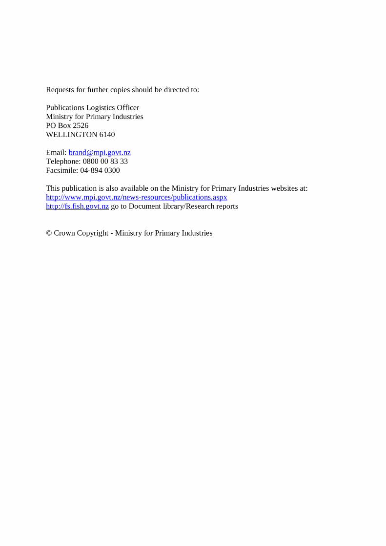
be used by fisheries management to develop approaches which maintain the resilience of individuals, populations, communities of fish, and marine ecosystems to the combined and interacting effects of climate and fishing. Perry et al. (2010) suggests that resilience can be enhanced by (1) maintaining demographic structure in fish population i.e. maintain large (older) individuals in exploited populations; (2) maintaining spatial structure in fish populations: hence, use indicators to track changes in the spatial distribution of exploited species, with a decrease in spatial structure being negative; (3) maintaining life history traits in exploited fishes, i.e. use indicators such as growth rate and age-at-maturity in target species; (4) maintaining buffering capacity of populations to environmental and ecosystem variability by keeping populations larger; (5) maintaining functional biodiversity in middle trophic level groups. There are many processes by which climate and oceanographic change can affect deepwater communities and fisheries (Rijnsdorp et al. 2009, Hollowed et al. 2013). The effects can be grouped as: (1) direct effects of abiotic changes in the environment on adult deepwater fish; (2) changes in the ecosystem carrying capacity via changes at some or all ecosystem levels from primary producers to predators of deepwater fishes; (3) effects on recruitment of deepwater fishes due to biotic and abiotic factors affecting spawning, eggs and juveniles. A schematic of potential effects of climate change on ecosystems is given in Figure 1 (Hollowed et al. 2013, Figure 2). In the New Zealand region, the direct effects of abiotic oceanographic change on deepwater species are likely to be less important than effects on juveniles as changes to the coastal environment due to climate are likely to be greater than changes in deep waters. The effect of climate change on the marine ecosystems of which deepwater fish are part, and particularly on the ecosystem services which provide prey for deepwater fishes, are not known. Hence, in Sections 3 (Climate indices), 4 (Oceanographic indices), 5 (Primary productivity) and 6 (Food-web indicators) we identify potential indicators of change in these abiotic and biotic components. Further research is needed to establish mechanistic links between variation in these indices and particular deepwater species or fisheries. Even without this knowledge, ongoing observation of changes in the oceanographic environment, or patterns of primary production, in the regions where important deepwater fisheries occur would provide context for interpreting changes in deepwater stocks and may give early warning of a climate-mediated regime shift.
10 • Ecosystem and environmental indicators for deepwater fisheries Ministry for Primary Industries
Figure 1: Conceptual pathways of direct and indirect effects of climate change and other anthropogenic factors on marine ecosystems, with their implications for adaptation and management. Solid arrows, consequences of climate change; dotted arrows, feedback routes (adapted from Hollowed et al., 2013, figure 2).
2.2 Criteria for evaluating indicators A number of previous reviews have provided criteria for evaluating the usefulness and robustness of ecosystem and environmental indicators (CGER 2000, Jackson et al. 2000, ICES 2001, Shin et al. 2010) but these are related to the purpose of the indicators. In general, good ecosystem indicators should be easily measured, cost effective to collect and calculate, easily interpreted (to avoid confusion about the state of the system they are reflecting) and directly applicable to management targets. The criteria for individual indicators include that they should be:
• Nationally significant – Does the indicator give information at the scale of the New Zealand EEZ? If more regionally based, is the region of national importance?
• Relevant – Is the indicator measuring something of importance in terms of manageable fisheries activity and progress towards sustainability?
• Credible – Are the underlying data, methodology and assumptions scientifically robust? Does the indicator stand up to scientific scrutiny as unambiguously measuring progress towards sustainability?
• Interpretable – Will non-technical stakeholders be able to interpret what the indicator is showing? Are historical trends available to allow the indicator to be put in a medium-term context?
• Cost-effective – Are the data required available in a timely fashion? Is it likely that data will continue to be collected in the medium to long term? How much additional data/research is required to develop the indicator?
• Internationally comparable – Have similar indicators been used overseas so that New Zealand performance can be benchmarked against international experience?

Ministry for Primary Industries Ecosystem and environmental indicators for deepwater fisheries • 11
In addition to these, with specific relevance to the objectives of this study, we would add:
• Is the indicator of relevance to deepwater fisheries and environments (deeper than 200 m)?
A number of studies have previously identified that a suite of indicators are required to monitor the broad range of ecological aspects of interest for management (CGER 2000, ICES 2001, Fulton et al. 2004, Tuck et al. 2009), and therefore we also add:
• Does the range of indicators adopted for routine use need to provide comprehensive coverage of all aspects of ecosystem dynamics that could be affected by fishing, or could affect fisheries productivity.
2.2.1 Indicator reference points, envelopes and directions A wide range of previous studies have recognised the value of some form of reference level to measure indicators against (Cury & Christensen 2005, Jennings & Dulvy 2005, Greenstreet & Rogers 2006). However, even within the European Union, where Ecological Quality Objectives have been defined, progress towards reference points has been slow and difficult. This partly derives from the difficulty in establishing reference levels, the metric value expected in the absence of human activity, and also deciding a metric level that is consistent with good ecosystem governance, yet still permits the continuance of a viable fishing industry (Greenstreet & Rogers 2006). While the first component of this relates to our understanding of marine ecology, the second is primarily a political issue, with significant social implications (Jennings & Dulvy 2005). Other than for commercial fish stocks, reference levels for ecosystem components are generally lacking. A recent EU project (IMAGE 2010) developed simulation models to calculate common fish community indicators, and similar approaches have also been adopted elsewhere (Fulton et al. 2011). These studies have concluded that identification of reference values is far from a trivial exercise, often requiring development of extensive simulation models (with associated demands on knowledge and data), and that universal reference levels are unlikely to work, as different systems are under different pressures and respond in different ways. Where sufficient knowledge is lacking to establish reference levels for indicators, trends and reference directions may offer an alternative (Jennings & Dulvy 2005). Expected directions of change for particular indicators can be determined in relation to pressures, although recent studies have shown a lack of consistency in trends both within and between exploited ecosystems, potentially reflecting different historical patterns of exploitation, management and environmental regimes (Blanchard et al. 2010). Within this report we have not attempted to identify reference levels for indicators, but have identified expected directions for key recommended indicators, in relation to pressures (see Table 3).
2.3 DPSIR framework Indicators are often classified using the Driver-Pressure-State-Impact-Response (DPSIR) framework (Figure 2) (Garcia & Staples 2000), and in developing a suite of indicators it may be useful to try to draw from across this framework where possible. Within this framework,

12 • Ecosystem and environmental indicators for deepwater fisheries Ministry for Primary Industries
human driving forces Driver (e.g., demand for food and revenue, economic and demographic forces, industrial development) exert Pressure on the environment (e.g., use of resources, impacts on habitat, generation of waste, pollution, climate change). Natural cycles (e.g., Inter-Decadal Pacific Oscillation) may also be considered as drivers, exerting pressures on the environment. These pressures may result in changes in the State of the components of the system and its environment (e.g. decreases in resource biomass, or revenues in coastal regions, ocean acidification, changes in ocean circulation), and may have an Impact on the functioning of the system (e.g. collapse of fishery, reduction in biodiversity, social unrest). Societies, possibly through management authorities, provide a Response to these changes of state and impacts (e.g., legal, institutional or financial measures, changes in development strategies) with a view to modify the pressure or mitigate its effects. Within this study, we have not considered Driver indicators explicitly. It can be difficult to differentiate whether an indicator falls into the State or Impact categories, and these are often combined. Adopting the DPSIR framework (and not considering the social drivers), the indicators fall into Pressure (exerted by human activities), changes in the State of components of the system, Impact (effects) and Response (of society and management) groupings. Most previous reviews have largely focussed on the State and Impact indicators, often dealing with them as a combined group, and have categorised them in different ways, either based on the scales the indicators consider (individual, population, community, ecosystem) or the ecological aspect addressed (environment, species-based, size-based, trophodynamic).
Figure 2: DPSIR framework. Arrows reflect directions of pressure.
While the DPSIR framework provides a useful mechanism by which the links between different types of indicator can be visualised, there can be considerable overlap between areas, with indicators related to a particular topic appearing in different components of the framework. For example, fishing effort and catches are pressures, stock abundance and fish community composition are states, while management actions are responses. To avoid fragmentation, here, indicators are grouped within topic area (see below), although classification within the DPSIR framework is also identified where appropriate.

Ministry for Primary Industries Ecosystem and environmental indicators for deepwater fisheries • 13
Recommended practice in terms of indicator use is to develop a comprehensive suite of indicators covering all aspects of ecosystem dynamics, and to that end, we have attempted to identify the key aspects of the environment that should be considered, and where appropriate, identify indicators for each of these addressing the different components of the DPSIR framework.
2.4 Indicators grouped by topic area Fulton et al. (2004, 2005) evaluated the performance of ecological indicators to detect the effects of fishing, within simulation models based on the Atlantis framework. They concluded that a suite of indicators are required, each focussing on different ecosystem attributes, and spanning different groups and processes. The main biological groups that need to be included are:
• Groups at the base of the food-web responsible for the primary fixation of organic matter (and energy) into the marine food-web, and for the transfer of material to small consumers with fast turnover (e.g., zooplankton, bacteria). These groups may be expected to respond quickly to change in the system and may act as early warning indicators of climate and oceanographic change that may affect fish and fisheries.
• Groups targeted by fisheries – the part of the foodweb most directly impacted by
fishing activity.
• Middle-trophic level groups that link the primary producers and bottom end of the food-web with fish. These include pelagic and hyperbenthic crustaceans (especially copepods, euphausiids, decapods and amphipods), gelatinous or soft-bodied groups (jellyfish, salps, polychaetes), cephalopods (squid and octopus), larval and juvenile fish (ichthyoplankton), and small pelagic adult fishes (especially myctophids).
• Habitat defining groups. These may play a critical role in structuring benthic communities and may provide crucial habitat for larval fishes. The deep-sea benthic community may also be a good proxy for overall biodiversity.
• Charismatic (or sensitive) groups, including top piscine predators (like sharks, rays, tuna) and air-breathing predators (seabirds and marine mammals). These groups, at the top of the food chain, tend to have slow dynamics. These groups can act as integrators of change, and be informative on underlying ecosystem state (Reid et al. 2005, Constable 2006).
Community- and ecosystem- level indicators were usually the most informative (Fulton et al. 2005). In general, population-level indicators appeared to be too sensitive to short-term fluctuations or species specific factors to be effective indicators for integrated community- and ecosystem- level attributes. Indicator responsiveness (which declines from population to community to ecosystem) is important in the management context, suggesting that community indicators provide a compromise between data requirements, signal strength, and sensitivity to natural variability (Fulton et al. 2005). In the absence of any specific New Zealand legislative guidance on the coverage of indicators, we have examined the European Marine Strategy Framework Directive (MSFD;

14 • Ecosystem and environmental indicators for deepwater fisheries Ministry for Primary Industries
2008/56/EC) and other international approaches (Fulton et al. 2004, State of the Environment Committee 2011) to identify a list of categories over which we identify and review indicators. Indicators have been grouped into eight sections as follows:
Section 3: Climate Indices Section 4: Oceanographic Indices Section 5: Primary productivity Section 6: Food-web indicators Section 7: Fisheries and fisheries management indicators Section 8: Fish community Section 9: Benthic community and habitats (sea-floor integrity) Section 10: Top predators and threatened/protected species
These categories of indicators encompass influences on the ecosystem (“pressures”) (Environmental conditions and Fishing activities), and measures of the state of the main components of the ecosystem for which data are available (Fish, Benthic communities and habitats, Plankton, and Top predators, (sharks and rays, seabirds, marine mammals)). These components of the ecosystem encompass the main biological groups identified by Fulton et al. (2005), focussing on different ecosystem attributes, and spanning different groups and processes. Most ecosystem component indicators to date have focussed on the fish communities, since these generally have the most data available.
3 CLIMATE INDICES Open ocean ecosystems, including those of which deepwater fisheries are part, are affected by natural interannual climate variability. This can result in changes in the frequency, magnitude, or timing of water column mixing and stratification, and primary production which may lead to marked changes in the organisation of the whole ecosystem (Fasham et al. 2001). The state of the New Zealand climate has important effects on the regional oceanography and hence marine ecosystems. Pressures relating to climate change have been identified as having a substantial potential effect on New Zealand marine ecosystems (MacDiarmid et al. 2012). Natural variability and cycles in climate forcing, coupled with human-induced effects on global climate, have profound implications for management of sustainable harvesting of ocean living resources. Climate-induced changes to oceans will include rising sea levels, changes to upwelling and ocean circulation regimes, water column stratification changes (of particular relevance to many coral and sponge species), ocean acidification, and warmer ocean temperatures. Globally, a number of climate and oceanographic indices have been found to be correlated with fish population processes, and have been used to identify evidence of environmental regime shifts. Recently, recognising that climate and regional oceanography may be linked to recruitment strength and, potentially, population biomass in some fish species (Dunn et al. 2009b), several indicators of climate and oceanographic state of the New Zealand EEZ have been brought together to provide background environmental data relevant to fisheries management (Dunn et al. 2009b, Hurst et al. 2012).

Ministry for Primary Industries Ecosystem and environmental indicators for deepwater fisheries • 15
3.1 Interdecadal Pacific Oscillation (IPO) The Interdecadal Pacific Oscillation (IPO, also called the Pacific Decadal Oscillation, PDO) is a 15–30-year cycle that affects parts of the Pacific Basin, causing variability in climate, including sea temperature, and has substantial and long-lasting effects on regional ecosystems. For example, under the IPO variation, community structure in the Gulf of Alaska ecosystem changed dramatically and abruptly after the climate regime shift of 1976/77 from a cold regime to a warm one (Anderson & Piatt 1999). Over a 40-year study period, prey species such as pandalid shrimp (three species) and capelin were the dominant species until 1976; after 1977, recruitment of predatory fish increased and, by the 1980s, these prey species had essentially disappeared. Total biomass in the standardised survey catches increased by over 250% (Kennedy et al. 2002). In a broader survey of the biological effects of the 1970s climate shift, Francis et al. (1998) documented major changes in the large marine ecosystems of the northeast Pacific, including abrupt population increases (and decreases) for zooplankton, fish, birds, and marine mammals. Although the exact mechanism by which these changes occurred is unknown and probably differs between species, the driving force behind these widespread ecosystem modifications was climate variability (Kennedy et al. 2002). Figure 3 shows the variations in the IPO derived from global sea surface temperatures. New Zealand experienced significant climate cooling in 1950 and again in 1977, after which the pattern shifted to a warmer phase. Between 1978 and 1998, El Niño events increased and there has been much debate about whether this was a result of global warming or due to natural variations in the climate over decades (10-year periods) (Mullan et al. 2009).
Figure 3: Interdecadal Pacific Oscillation index based on Mullan et al. (2009). This index is also called the Pacific Decadal Oscillation (PDO).

16 • Ecosystem and environmental indicators for deepwater fisheries Ministry for Primary Industries
3.2 Southern Oscillation Index (SOI) The Southern Oscillation Index (SOI) is the normalized mean sea surface pressure difference between Tahiti and Darwin (Australia) (after Trenberth 1984). SOI data may be sourced from the National Climate Center (NCC) of the Australian Bureau of Meteorology, with a climate base period from 1933 to 1992 (Allan et al. 1996). SOI data are often smoothed using a five-month running mean (Ropelewski & Jones 1987, Jiang et al. 2006). The SOI is related to the strength of the trade winds in the Southern Hemisphere tropical Pacific (Mullan 1995) and SOI values for May-September are often used as an indicator of El Niño-La Niña Southern oscillation (ENSO, Trenberth 1997). There are two phases of ENSO — El Niño (warm ENSO phase) and La Niña (cool ENSO phase). El Niño refers to the appearance of anomalously warm waters extending west of the International Dateline. Off the west coast of South America, this results in the disappearance of cool nutrient-rich upwelled water. La Niña represents the appearance of anomalously cool waters in the same region of the Pacific, with upwelling enhanced. A year is often defined as a La Niña year if at least one SOI value for May-September is equal to 1 or more; if there is at least one SOI value less than or equal to -1, the year can be defined as an El Niño year; in all other cases, the year is considered “Normal” (Figure 4). Jiang et al. (2006) found this definition to be consistent with the season-by-season breakdown list of occurrences of ENSO events provided by the USA's National Center for Environmental Prediction (NCEP 1999). In the New Zealand region, the SOI is correlated with rainfall, wind, temperature and oceanography (Figure 5) (Basher & Thompson 1996, Salinger & Mullan 1999).
Figure 4: Southern Oscillation index based on Mullan et al. (2009).

Ministry for Primary Industries Ecosystem and environmental indicators for deepwater fisheries • 17
Figure 5: Pattern of air pressure and wind direction during El Niño and La Niña phases of the Southern Oscillation. During the El Niño phase, pressures are high (H) to the north. Strong south-westerly winds bring drought to the north-east of the country. When La Niña is operating, there are high pressures over the South Island. These bring north-easterlies and rain to the north and east of the North Island.
3.3 Antarctic Oscillation The Antarctic Oscillation (AAO, also known as the High Latitude Mode or Southern Annular Mode) is the alternate weakening (negative phase) and strengthening (positive phase) of the westerlies, roughly every month (Figure 6). The AAO is the dominant pattern of non-seasonal tropospheric circulation variations south of 20°S (Thompson & Wallace 2000). Over the last 30 years there has been a trend towards a stronger positive phase – stronger westerly winds at latitude 50° south which has been attributed to increased greenhouse gases and ozone depletion in the stratosphere (Mullan et al. 2009).

18 • Ecosystem and environmental indicators for deepwater fisheries Ministry for Primary Industries
Figure 6: Antarctic Oscillation index (AAO). Top three panels: AAO for the period 1980–2012, with 3-month running mean. Bottom panel: Daily AAO for 2012 (Source: www.cpc.ncep.noaa.gov/products/precip/CWlink/daily_ao_index/aao/aao_index.html).

Ministry for Primary Industries Ecosystem and environmental indicators for deepwater fisheries • 19
3.4 Kidson weather types A number of methods have been used to identify and classify representative weather types, including subjective classification methods (e.g., Lamb 1950), correlation analysis (Lund 1963), sums-of-squares (Kirchhofer 1973, Blair 1998), cluster analysis (e.g., Key & Crane 1986, Kidson 1994a), and principal component analysis (PCA) (Richman 1981, Huth 1996), with no objective method being indisputably superior (Huth 1995). For the New Zealand region, early subjective methods (Kidson 1994a) were followed by a combination of empirical orthogonal function analysis and clustering techniques (e.g., Kidson 1994b, Kidson & Watterson 1995, Kidson 1997, 2000) leading to “Kidson regimes” (Kidson 2000, Renwick 2011). These Kidson regimes give the occurrence of 12 different characteristic types of weather pattern over New Zealand. More recently, principal component analysis (Preisendorfer 1988) was used to characterise ten synoptic weather types, and analyse the occurrence of these types in relation to different phases of the SOI (Jiang et al. 2006).
3.5 Ocean winds Winds are intimately related to regional oceanography, through effects on currents, fronts, water column structure (including mixed layer depth), upwelling, mesoscale eddy structure, and surface waves (e.g., Small et al. 2008, Chelton & Xie 2010). Three methods can be used to observe and/or estimate ocean winds in the New Zealand region:
• Direct measurement of winds close to the sea surface from anemometers on vessels and coastal weather stations (e.g. Auckland airport; meteorological network). Microwave radar can also be used to measure wind speeds from vessels if high frequency or stratified observation is required.
• Analysis of numerical atmosphere and weather models. Analysis of long term
variations in ocean winds at a global scale based on weather prediction/assimilation models has been conducted by the US National Center for Environmental Protection–National Center for Atmospheric Research (NCEP–NCAR) and is known as the “NCEP–NCAR reanalysis wind fields” and is available online: http://www.esrl.noaa.gov/psd/data/. These reanalyses are continually being updated.
• Satellite measurements of ocean winds. A number of methods are presently used to
estimate winds from Earth-observing satellites, including tracking features (clouds and water vapour) in geostationary and polar imagery sequences and ocean surface winds derived from radar backscatter and conical-scanning microwave radiometers (typically called “scatterometers”). Future approaches to satellite measurement of ocean winds include using data from the Multi-angle Imaging Spectroradiometer (MISR), wind profile information from space-borne lidar and 3-D wind fields derived from tracking features in clear sky moisture fields produced from future geostationary hyperspectral infrared sounders. The most commonly used ocean-surface wind product from satellites obtained is probably from the NASA Quick Scatterometer, QuikSCAT. The 8-year QuikSCAT record (September 1999–August 2007) has been used to develop an atlas of 12 wind variables, including zonal and meridional winds, wind stress and wind stress derivative (curl and divergence) fields: Scatterometer Climatology of Ocean Winds (SCOW), available at: http://cioss.coas.oregonstate.edu/scow/ . Global estimates of seasonal cycles of the

20 • Ecosystem and environmental indicators for deepwater fisheries Ministry for Primary Industries
wind and wind stress fields from the NCEP–NCAR reanalysis have been compared to SCOW seasonal cycles. The SCOW atlas is able to capture small-scale features that are dynamically important to the ocean but are not resolved in other observationally based wind atlases or in NCEP–NCAR reanalysis fields (Risien & Chelton 2008).
3.6 Recommended candidate Climate indicators Climate indices should form a key part of the suite of indicators for deepwater fisheries, to provide some broader scale environmental context to changes seen in other datasets. Indicators that are regularly updated will be the most cost-effective and these include:
• Southern Oscillation Index (SOI) • Interdecadal Pacific Oscillation (IPO) • Antarctic Oscillation (AAO)
More New Zealand region focussed indicators (that are less regularly updated) include:
• Kidson weather types • Ocean winds
4 OCEANOGRAPHIC INDICES Abiotic environmental drivers can impact ecosystems at least as strongly as fishing (Schiermeier 2004, Frank et al. 2007, Mackinson et al. 2009), and can act synergistically with fishing to cause long-term change in marine ecosystems (Winder & Schindler 2004, Kirby et al. 2009). Observation of oceanographic change in regions where life stages of deepwater fishes occur will provide context to understanding change in stocks, including the potential effect of regime shift. Oceanographic state and variability are likely to become increasingly important drivers of marine ecosystem change in New Zealand in the medium to long term, as global climate change continues (Willis et al. 2007, Polunin 2008). Effects may be manifested through inter alia warming of ocean waters affecting species biology and ecology (Perry et al. 2005, O'Connor et al. 2007), regime shifts (large-scale and persistent changes in ocean circulation and vertical water column structure (Mullan et al. 2001)), increased likelihood of invasive species (Willis et al. 2007), increasing ocean acidification (Fabry et al. 2008, Cooley & Doney 2009b), and effects across multiple trophic levels due to timing of productivity (Sydeman & Bograd 2009). Three general types of approach are commonly available for observing, monitoring and understanding changes in regional oceanography (i.e. appropriate to the scale of the New Zealand EEZ): (1) satellite based methods; (2) in situ observations, including measurements from research vessels, measurements from ships of opportunity (e.g. expendable bathythermographs), moorings and drifters; (3) numerical models, including those which assimilate satellite and in situ observations. These are discussed in relation to ocean temperature and circulation below.
Ministry for Primary Industries Ecosystem and environmental indicators for deepwater fisheries • 21
4.1 Ocean temperature
4.1.1 Impacts of temperature change on ocean communities Marine organisms, communities and ecosystems may be impacted in several important ways by ocean warming (e.g., Rijnsdorp et al. 2009, Hollowed et al. 2013). Changes in temperature can alter the number and diversity of adult species in a certain area, by changing larval development time and dispersion (O'Connor et al. 2007), lead to changes in biodiversity through invasive species, and altering ecosystem structure and function through changing production and consumption rates of marine organisms. Several groups rely on zooplankton as their primary food source, and warmer water may reduce the availability of zooplankton through increased grazing rates, and also change the zooplankton species community composition, through different temperature preferences, which may have knock on effects for predators.
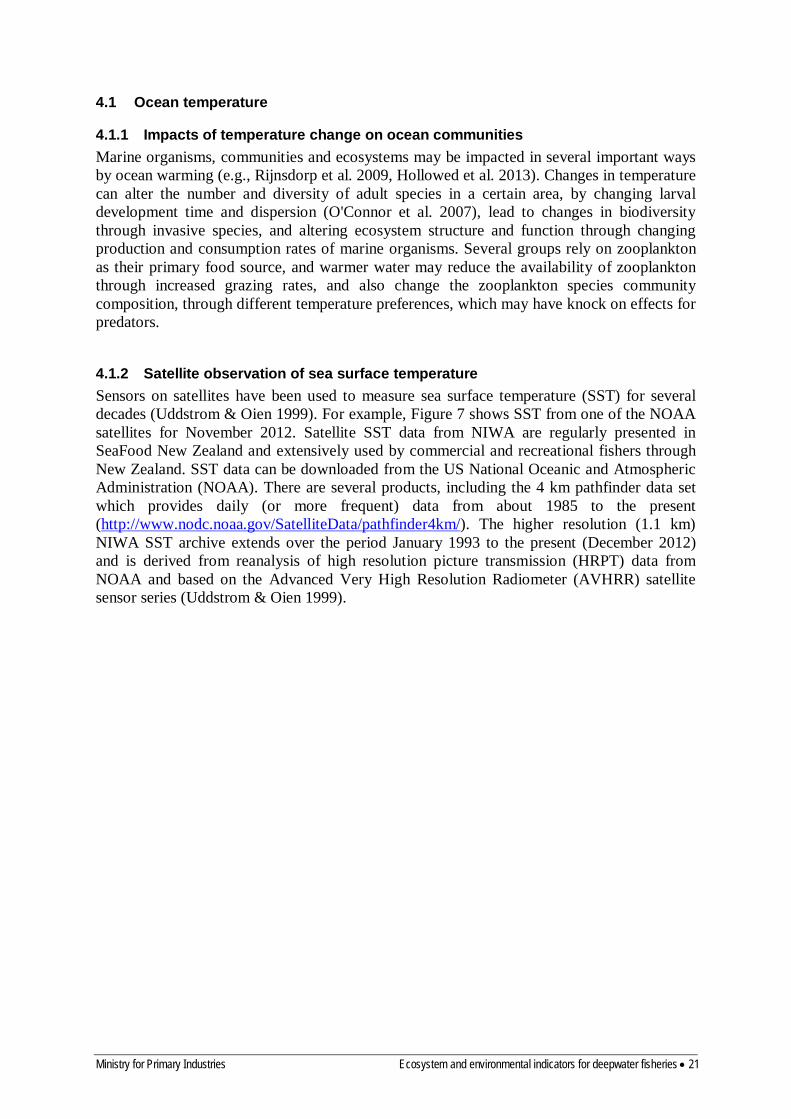
4.1.2 Satellite observation of sea surface temperature Sensors on satellites have been used to measure sea surface temperature (SST) for several decades (Uddstrom & Oien 1999). For example, Figure 7 shows SST from one of the NOAA satellites for November 2012. Satellite SST data from NIWA are regularly presented in SeaFood New Zealand and extensively used by commercial and recreational fishers through New Zealand. SST data can be downloaded from the US National Oceanic and Atmospheric Administration (NOAA). There are several products, including the 4 km pathfinder data set which provides daily (or more frequent) data from about 1985 to the present (http://www.nodc.noaa.gov/SatelliteData/pathfinder4km/). The higher resolution (1.1 km) NIWA SST archive extends over the period January 1993 to the present (December 2012) and is derived from reanalysis of high resolution picture transmission (HRPT) data from NOAA and based on the Advanced Very High Resolution Radiometer (AVHRR) satellite sensor series (Uddstrom & Oien 1999).

22 • Ecosystem and environmental indicators for deepwater fisheries Ministry for Primary Industries
Figure 7: Satellite derived sea surface temperature for the New Zealand region for 25–28 Nov 2012.
4.1.3 Bulk water temperature The most accurate measure of water temperature at depth is made using CTD (Conductivity Temperature Depth) instruments from research vessels. This instrument measures temperature and salinity profiles through the water column with high accuracy. For example, the SeaBird sensor as used on RV Tangaroa, has a specified accuracy of ±0.001°C, with a NIST-traceable calibration applying over the entire oceanographic range. The CTD is arguably the most fundamental oceanographic tool, and is deployed on almost all oceanographic research voyages to make temperature and salinity sections. In deep water, these sections can also be used to infer subsurface currents. Expendable bathythermographs (XBTs) have been deployed across the eastern Tasman Sea between 1991 and 2005 (Sutton et al. 2005). These instruments have lower accuracy but can be deployed from ships of opportunity (e.g. container ships) to measure vertical profiles of water temperature. The data from the Wellington-Australia transect show that the eastern Tasman Sea warmed between 1996 and 2002 (Figure 8), with this warming extending to the

Ministry for Primary Industries Ecosystem and environmental indicators for deepwater fisheries • 23
full depth of the sampled water column (i.e. to about 800 m). The in situ measurements of warming agreed with measurements from satellite sea surface temperature and sea surface height products.
Figure 8: Mean temperature in the Tasman Sea with depth and time. The survey times are indicated by the vertical bars along the top axis (Sutton et al. 2005).
4.1.4 Sea-bed temperature Average bottom temperature for the New Zealand region can be obtained from combining bathymetric data for the New Zealand region (e.g., CANZ 1996) with hydrographic climatologies (Figure 9). A number of such oceanographic climatologies exist including (1) the CSIRO Atlas of Regional Seas, CARS2000 (Dunn & Ridgway 2002); (2) World Ocean Atlas 2001 version 2. The latter dataset is published by the US National Oceanographic Data Center (http://www.nodc.noaa.gov/OC5/WOA01/qd_ts01.html) and was constructed by an objective analysis of in situ sub-surface ocean measurements, as described by Boyer et al. (2005). The World Ocean Atlas (0.25º grid) consists of objectively analysed grids at 0.25º spatial resolution interpolated onto 33 standardised depths from the surface to 5500 m. The accuracy of the World Ocean Atlas temperature field in the New Zealand region has never been quantified rigorously, but our informal comparisons with other data show that it describes the large-scale ocean features correctly (i.e. on spatial scales of about 200 km or more) but does not capture the finer-scale detail.

24 • Ecosystem and environmental indicators for deepwater fisheries Ministry for Primary Industries
Figure 9: Estimated temperature at the sea-bed produced by 3-dimensional interpolation of temperature-depth-location data onto a Mercator projection grid at 1 km resolution (Pinkerton et al. 2005).
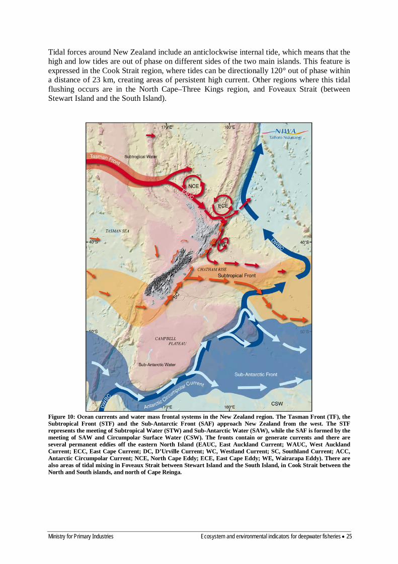
4.2 Ocean circulation Many and varied measurements of physical oceanography in the New Zealand region have been made over the last century, leading to the present understanding of flow in the region (Figure 10). In the south, New Zealand poses a barrier to the easterly flow of the Subtropical Convergence, where subtropical and sub-Antarctic water masses meet. This front intersects the bottom portion of the South Island, is deflected southwards along the shelf edge, turns northwards, following the Otago coast, and extends out along the Chatham Rise. This feature contributes to a change in the biological character of species in these areas. Towards the southern extreme of the New Zealand region, another major oceanic frontal system, the Antarctic Circumpolar Current, flows eastward along the edge of the Campbell Plateau.
Ministry for Primary Industries Ecosystem and environmental indicators for deepwater fisheries • 25
Tidal forces around New Zealand include an anticlockwise internal tide, which means that the high and low tides are out of phase on different sides of the two main islands. This feature is expressed in the Cook Strait region, where tides can be directionally 120° out of phase within a distance of 23 km, creating areas of persistent high current. Other regions where this tidal flushing occurs are in the North Cape–Three Kings region, and Foveaux Strait (between Stewart Island and the South Island).
Figure 10: Ocean currents and water mass frontal systems in the New Zealand region. The Tasman Front (TF), the Subtropical Front (STF) and the Sub-Antarctic Front (SAF) approach New Zealand from the west. The STF represents the meeting of Subtropical Water (STW) and Sub-Antarctic Water (SAW), while the SAF is formed by the meeting of SAW and Circumpolar Surface Water (CSW). The fronts contain or generate currents and there are several permanent eddies off the eastern North Island (EAUC, East Auckland Current; WAUC, West Auckland Current; ECC, East Cape Current; DC, D’Urville Current; WC, Westland Current; SC, Southland Current; ACC, Antarctic Circumpolar Current; NCE, North Cape Eddy; ECE, East Cape Eddy; WE, Wairarapa Eddy). There are also areas of tidal mixing in Foveaux Strait between Stewart Island and the South Island, in Cook Strait between the North and South islands, and north of Cape Reinga.

26 • Ecosystem and environmental indicators for deepwater fisheries Ministry for Primary Industries
Long time series of oceanic observations in the New Zealand are uncommon. Below, the major sets of measurements that are relevant to large-scale understanding and observation of ocean circulation in the New Zealand EEZ are listed.
4.2.1 Sea Surface Height from Satellite In deep water more than about 1000 m, sea surface height (SSH) can be viewed as analogous to pressure in the atmosphere, in that water flows along contours of SSH in what is called the geostrophic relationship. SSH anomalies (i.e., differences from the mean) have been determined from satellite radar altimeter measurements since the launch of the Topex/Poseidon (T/P) instrument in 1992. Since then, a number of other satellite altimetry sensors have become available, including Jason-1, ERS-1 and ERS-2, and EnviSat. The AVISO project collates, analyses and disseminates satellite altimetry data from these sensors, and merged SSH data can be downloaded from the AVISO website: http://www.aviso.oceanobs.com/. NIWA routinely collects the AVISO anomaly gridded products (Figure 11).
Figure 11: Sea surface height anomaly (m) for the New Zealand region from 1 January 2001 from AVISO merged dataset. Vectors show surface current anomalies corresponding to this anomaly.
4.2.2 Current measurements: Current meters Current meters have been deployed sporadically across the New Zealand EEZ for some time (Chiswell & Schiel 2001), although mostly for short durations. Most early deployments in New Zealand waters were of the rotating vane type (RCM), while more recently, these RCM meters have been replaced by acoustic meters, which tend to be more reliable. Current meter data are generally more useful for showing variability in the currents than measuring mean flows.

Ministry for Primary Industries Ecosystem and environmental indicators for deepwater fisheries • 27
4.2.3 Current measurements: Shipboard ADCP Acoustic Doppler Current Profilers (ADCPs) measure ocean current velocities by emitting pulses of sound and using the Doppler frequency shift of the returning echo to estimate the current speeds. Some early work with an ADCP was done on RV Rapuhia (Chiswell 1994). An ADCP has been installed on RV Tangaroa since 1996 and data are collected on selected voyages where there is no interference with other instruments (e.g. other acoustic sounders).
4.2.4 Current measurements: Global Drifters The Global Drifter Program (GDP) is designed to measure the world’s surface velocity using satellite-tracked Lagrangian drifters. These drifters are comprised of a surface float attached to a holey-sock drogue, and are designed to estimate the flow at a nominal depth of 15 m (Roemmich & Gilson 2009). The surface float contains a satellite Global Positioning System (GPS) unit and relays the drifter’s latitude and longitude via satellite to a central data facility. GDP drifters in the New Zealand region, although relatively sparse, can be used to estimate surface velocities. Figure 12 shows the tracks of drifters in the Chatham Rise region since the early 1990s. These drifter tracks can be averaged into latitude-longitude bins to compute the mean surface flow (Figure 13). GDP drifter data are available from the GDP Operations Center at http://www.aoml.noaa.gov/phod/dac/gdp_doc.php.
Figure 12: Example tracks of drifters in the New Zealand region since the early 1990s. All available drifter data are shown covering the period 1990 to 2010. Illustrative selected drifters are shown with blue tracks.

28 • Ecosystem and environmental indicators for deepwater fisheries Ministry for Primary Industries
Figure 13: Mean surface flow computed from the drifters passing through the New Zealand region.
4.3 Ocean Acidity There is little doubt that the ocean is undergoing dramatic changes, with increasing CO2 and changes in pH (Gattuso & Hansson 2011). This includes New Zealand waters, where acidification is measurable and changing (Currie et al. 2011, Feely et al. 2012). Over the next few decades ocean uptake of CO2, and its acidifying reaction with seawater, is expected to substantially decrease oceanic pH and the availability of carbonate ions (needed for calcification). Monitoring of oceanography, including acidity, has been carried out along a transect in sub-Antarctic waters off the Otago shelf for eight years (January 1998 to December 2005) – the “Munida” transect (Currie & Hunter 1999, Currie et al. 2011). Measurements of sea surface temperature, salinity, nutrient concentrations and pCO2 allowed the ocean-atmosphere flux of carbon dioxide along this transect to be calculated. Results indicate increasing ocean acidity in this region (Currie et al. 2011), but other than these limited areas around New Zealand, little sampling and monitoring of the ocean acidity has been carried out. Recently a revised map of our regions aragonite and saturation horizon zones has been produced (Figure 14)(Tracey et al. 2013). This map uses the relationships between hydrographic parameters (temperature, salinity and oxygen) and carbonate parameters (alkalinity and dissolved inorganic carbon) from a limited number of stations where it has been measured. It then uses these algorithms to estimate carbonate parameters from the CARS ocean climatology data for this region (Bostock et al. 2013, Tracey et al. 2013).

Ministry for Primary Industries Ecosystem and environmental indicators for deepwater fisheries • 29
Figure 14: Detailed aragonite saturation horizon (ASH, upper plot) and calcite saturation horizon (CSH, lower plot) maps using the algorithms and the CARS climatology for the New Zealand region. Plots show the depth of the respective horizons in metres. The location of the WOCE and NIWA stations where alkalinity and DIC were sampled are shown by black dots. The white regions in each plot represent topography shallower than the ASH and CSH (Tracey et al. 2013).
30 • Ecosystem and environmental indicators for deepwater fisheries Ministry for Primary Industries
Saturation states are dependent on the solubility of the mineral, which varies with temperature, salinity, pressure and the mineral phase. There are three main calcium carbonate (CaCO3) minerals found in nature; calcite, aragonite and high Mg calcite. Aragonite is 50% more soluble than calcite while high Mg calcite solubility is dependent on the amount of Mg. As Ca2+ is fairly constant in the oceans and directly proportional to salinity, the saturation state (Ω) is controlled by the amount of carbonate (CO3
2-). The carbonate concentration cannot be measured directly in the seawater (at least not yet), but it can be calculated from measurements of total alkalinity and dissolved inorganic carbon (DIC). If Ω is greater than 1, the ocean is supersaturated with respect to the mineral, while if Ω is less than 1, then the water is undersaturated and the mineral will start to dissolve. The depth at which Ω equals 1 is termed the saturation horizon. The aragonite saturation horizon (ASH) is significantly shallower (upper plot Figure 14) than the calcite saturation horizon (CSH) (lower plot Figure 14), due to the increased solubility of aragonite. The aragonite saturation horizon (ASH) is considered to be a primary control on the global spatial and depth distributions of habitat-building scleractinian corals, with 95% found in depths above the ASH. The potential impacts of increasing ocean acidity on marine fauna such as plankton, fish, crustaceans, and corals are not well understood (Gattuso & Hansson 2011), although deepwater corals have specifically been identified as being at particular risk (Turley et al. 2007, Guinotte & Fabry 2008, Tracey et al. 2013). Various habitat-forming species, along with several, but not all marine fauna from the high order predators to fish, echinoderms, molluscs, crustaceans and small plankton species (such as pteropods) are known to be vulnerable to changes in ocean acidity. Potential threats of ocean acidification to seafood and sustainable harvesting of ocean resources can be considered to be of two types: (1) direct impacts on commercially valuable species; (2) indirect effects via perturbations to the marine food web and habitat formers. The most direct effect on seafood is associated with the process of calcification, where many calcareous organisms will have problems forming their shells or exoskeletons in an ocean rich in CO2. Experimental evidence suggests that the reduced level of calcium carbonate saturation will result in certain marine organisms, including shellfish, echinoderms, and corals, having difficulty building and maintaining their external calcium carbonate skeletons (Orr et al. 2005). This, in turn, will make the species more vulnerable to subsequent impacts, such as increased temperature and predation. For example, the blue mussel Mytilus edulis and the Pacific oyster Crassostrea gigas have shown a decrease in calcification of 25% and 10% respectively for conditions projected for the end of the 21st century (Gazeau et al. 2007). However, the projection of laboratory results to the natural environment remains problematic, and the effects of acidification on many species of calcified organisms remains largely unknown (Gattuso & Hansson 2011). If the future predictions of the shallowing of the ASH eventuate, most corals that currently thrive between 800 to 1200 m in the New Zealand Exclusive Economic Zone (EEZ), will be below the carbonate saturation horizon by 2100. In addition to the effects on the ability of calcifying organisms to develop shells and exoskeletons, ocean acidification may also affect metabolism, reproduction, and habitat availability for a range of species, including some commercially important species of finfish (Cooley & Doney 2009b, 2009a). Laboratory and in situ experiments have shown effects on growth of plankton, fish larvae, fish otoliths, and krill. Studies have shown a decrease in

Ministry for Primary Industries Ecosystem and environmental indicators for deepwater fisheries • 31
reproductive potential and sperm motility, and a larval mortality increase under increased acidification. Where acidification impacts are accelerated, in the Arctic, Antarctic, and deep-sea regions, serious impacts are being seen earlier than the predicted scenario of acidity increasing by 100–150 % (pH reduction of 0.3–0.4) by 2100 (Caldeira & Wickett 2003, Feely et al. 2004). In the Southern Ocean the ASH is predicted to outcrop at the surface in winter by 2030 (McNeil & Matear 2008). The future success of marine predators, including commercially-important finfish, is likely to depend on their capacity to alter their food sources, and whether alternative prey, that are less affected by acidification, will be available (Cooley & Doney 2009b).
4.4 Hypoxia / Anoxia The global oceans have pockets called “dead zones” which are areas experiencing sustained anoxic/hypoxic (no/low oxygen) conditions (Diaz & Rosenberg 2008). These pockets are increasing in size and frequency where there is lack of water motion, which may be affected by temperature through the thermohaline forces that create currents. Most oxygen-minimum zones (OMZs) are features of the pelagic region, but some intersect the benthos, thereby impacting a diverse fauna, and where the OMZs are seen as a threat to deep-sea corals and other cnidarians intolerant to anoxic conditions (Fautin & Eash-Loucks 2012). Recent research in the Pacific has indicated that sponges too are very tolerant to hypoxic, but not anoxic, conditions (Whitney et al. 2005). In the New Zealand region, dead zones have been found in the coastal zone, for example, in the Bay of Plenty following mangrove removal (Morton 2011) but to date no dead zones have been reported offshore.
4.5 Recommended candidate Oceanographic indicators As with the climate indicators discussed above, the state of the regional New Zealand oceanography should form a key part of the suite of indicators, providing context to help to interpret and understand any changes observed in biological indicators. Indicators of oceanographic state that can be obtained at regional scales, that are available from remote sensing approaches and do not require field data include:
• Sea surface temperature • Circulation derived from sea surface height
Indicators requiring ongoing field data acquisition include:
• Bulk water temperature • Anoxia • Water column structure • Nutrients • Ocean acidification
Remote sensing based indicators are likely to be more cost-effective, but some parameters cannot be measured remotely, and will require field data acquisition, with the associated additional costs.

32 • Ecosystem and environmental indicators for deepwater fisheries Ministry for Primary Industries
5 PRIMARY PRODUCTIVITY The growth of phytoplankton in the upper layers of the ocean provides the vast majority of the energy that fuels marine ecosystems. Near the coast, and in localised special areas, organic matter is formed by other primary producers, including macroalgae, seagrass, mangroves, epiphytes, autotrophic periphytes, microphytobenthos and chemosynthesisers. However, overall, photosynthesis by phytoplankton is the dominant source of energy in the marine realm, and is hence the focus of this section. Research is required to elucidate the mechanisms by which changes in primary production may affect deepwater fisheries in the New Zealand region, including identifying regions, times and characteristics of primary production which are of particular importance to the ecological viability of deepwater fish communities. Further research is also needed to estimate thresholds of limits of change for management. In the meantime, even in the absence of such a mechanistic understanding or quantititive reference points, monitoring for changes in the magnitude and patterns of primary production in the regions where deepwater fisheries and early-life stages of deepwater species occur is likely to provide valuable context for understanding change in deepwater fish stocks. Any substantial changes (including trends) in patterns of primary production are likely to underline the importance of further research on how change to the base of the foodweb may affect fished species.
5.1 Phytoplankton biomass
5.1.1 Satellite measurements of ocean colour Phytoplankton biomass is often quantified in terms of a vertically-integrated mass of organic carbon in phytoplankton cells (units of gC m-2). This can be measured accurately (within a few percent) from laboratory measurements of water samples collected from various depths on research voyages. As phytoplankton biomass varies substantially over very large ranges of time (minutes to decades) and space (centimetres to thousands of kilometres), in situ measurements are not able to quantify biomass at basin scales or monitor for change at decadal scales. Instead, satellite measurements of ocean colour provide an acceptable estimate of the concentration of chlorophyll-a (the ubiquitous phytoplankton pigment) in the surface ocean, which is an effective proxy for phytoplankton biomass (Hooker et al. 1992). The satellite-based method of observing, characterising and monitoring phytoplankton biomass has become standard for management and research purposes at moderate to large spatial and temporal scales (tens to thousands of kilometres; weeks to decades). The accuracy of the satellite based method (typically a target accuracy of within 35%) is much less than in situ methods, and periodic research and validation voyages in regions like the New Zealand EEZ are required to ensure that this target accuracy is being achieved and that data are fit for purpose.
5.1.2 Ocean colour satellite sensors More than 12 years (1997–present) of satellite measurements of ocean colour are currently available. Two ocean colour satellite sensors are used most often: OrbImage Sea Viewing Wide Field-of-view Sensor (SeaWiFS) covering September 1997 to 2010 and the NASA Moderate Resolution Imaging Spectroradiometer (MODIS-Aqua), providing data from 2002 to the present. Earlier measurements of ocean colour by the Coastal Zone Color Scanner, 1979–1986, had inadequate sensor characterisation, untracked sensor degradation and limited

Ministry for Primary Industries Ecosystem and environmental indicators for deepwater fisheries • 33
atmospheric correction, and are not considered here. SeaWiFS and MODIS-Aqua sensors are preferred over the MODIS-Terra sensor (operational between 2000 and ongoing as of mid-2013) because MODIS-Terra has poor sensor characterisation and system performance. In the New Zealand region, SeaWiFs provided data at a spatial resolution of 4 km (occasional data at 1 km) between 01/08/97 and 14/02/11. MODIS-Aqua (in operation from 4 May 2002) provides data at 1 km resolution, with some nearshore products available at 500 m and 250 m resolution. Satellite ocean colour data availability is limited by cloud cover and often monthly composite images are used, where all valid data measured during a given month are combined. Composite images do not give true mean monthly values because image pixels in different areas are composited from different quantities of data. Short-lived phytoplankton blooms (a few days) may have been missed completely or may disproportionately affect the composite value, especially when there were few cloud-free days (Comiso et al. 1993). In the New Zealand region, typically 10–30% of images are cloud-free, depending on location and season. The long-term mean based on satellite data can be biased if the property observed is correlated with the probability of observation. It is also noted that ocean colour data availability in sub-Antarctic waters during the winter is limited by solar elevation and persistent cloud cover.
5.1.3 Satellite ocean colour algorithms Satellite ocean colour sensors measure upward radiance at the top of the atmosphere in several discrete wavelength bands spanning the visible part of the spectrum (wavelengths 400–700 nm). Further measurements in the near infra-red (wavelengths between 700–1000 nm) are used to correct top-of-atmosphere measurements for light scattering in the atmosphere by gases and aerosols, and hence estimate normalised water-leaving radiance (Gordon et al. 1988) – the intensity of light leaving the surface of the water corrected to a standard viewing and lighting geometry. A single measurement of normalised water-leaving radiance constitutes a single measurement of "ocean colour". Various algorithms have been developed to estimate the near-surface concentration of Chl-a from each ocean colour measurement (e.g., O'Reilly et al. 1998). Open ocean waters are known as “Case 1” meaning that the colour of the water is dependent mainly on phytoplankton and their associated products. The change in the ratio of blue and green light exiting the water surface hence gives a reasonably-accurate measurement of Chl-a in these oceanic waters (O'Reilly et al. 1998). These are called “band-ratio” algorithms. The SeaWiFS and MODIS-Aqua missions aimed to measure Chl-a with less than 35% error, and this seems to be achieved in New Zealand oceanic (offshore) waters using standard band-ratio algorithms (Pinkerton et al. 2005). Simple methods of estimating Chl-a in oceanic waters using band-ratio algorithms will fail in coastal waters because the method does not separate the influence of different coloured material, such as phytoplankton, suspended sediment, and coloured dissolved organic matter (CDOM) (e.g., Aiken et al. 1995). Band-ratio algorithms can also fail if the local bio-optical conditions (e.g., chlorophyll-specific absorption) are unusual compared to measurements used to develop the algorithm (Morel & Maritorena 2001), or if highly-reflecting phytoplankton-detrital material is present (e.g. liths shed from senescent coccolithophore blooms) (Balch et al. 1991). These optically-complex waters, which are typical for New Zealand coastal waters and some offshore waters, are called Case 2. The presence of even moderate concentrations of suspended sediment (more than 1 g m-3) can also invalidate atmospheric correction methods that rely on the waters being dark in the near infra-red part of

34 • Ecosystem and environmental indicators for deepwater fisheries Ministry for Primary Industries
the spectrum (e.g., Lavender et al. 2005). Although a number of “prototype” methods exist for correcting for atmospheric effects when sediment is present (e.g., Lavender et al. 2005, Wang & Shi 2005, Schroeder et al. 2007) Pinkerton,unpublished data), none of these has advanced to become an accepted community standard. Similarly, a large number of prototype Case 2 in-water algorithms exist (e.g., Garver & Siegel 1997, Lee et al. 2002, Pinkerton et al. 2006), and some are available through the latest versions of the NASA ocean colour processing software, SeaDAS. However, because the optical properties of material in natural waters can vary regionally, local validation is required for confidence in the derived Case 2 products, and local tuning may be required for acceptable accuracy. Such work is been underway in New Zealand (e.g., Richardson et al. 2005, Pinkerton et al. 2006) and improved, operational ocean colour products may be available for the New Zealand coastal zone in the near future. At present however, ocean colour products of the New Zealand coastal zone should be interpreted with caution.
5.1.4 Patterns in climatological chlorophyll-a A summary of patterns in Chl-a from SeaWiFS measurements in the New Zealand EEZ between 1997 and 2000 is given in Murphy et al. (2001), with some subsequent validation (Pinkerton et al. 2005). More recently, Chiswell et al. (2013) examined the 13-year time-series of Chl-a derived from SeaWiFS in the New Zealand region. The mean near-surface Chl-a is elevated in the Subtropical Front and around the sub-Antarctic islands that have an associated shelf (Figure 15). Note that elevated Chl-a around the New Zealand coast is probably indicative of suspended sediment as well as potentially elevated phytoplankton biomass in these areas, as explained above. The annual cycle in surface Chl-a shows a ubiquitous unimodal summer bloom in sub-Antarctic water; autumn, winter and spring blooms occur variously in Subtropical waters and across the Subtropical Front (Figure 16). The autumn and winter blooms progress equator-wards with time and develop in response to deepening of the mixed layer; spring blooms show significant spatial structure and are different from year to year (Chiswell et al. 2013). Preliminary rotated empirical orthogonality function analysis (EOF) of satellite ocean colour data over the north-east New Zealand shelf has been completed (Richardson et al. 2002, Kennan & Pinkerton 2008), and the analysis has been extended to the EEZ-scale. EOF analysis can be carried out in a number of ways. Figure 17 shows EOF analysis of the annual cycle of Chl-a in the New Zealand region to investigate patterns in the spatial and monthly variability of Chl-a with all years of data combined (based on monthly composites). In this analysis, the first EOF capturing 50% of the variance, shows a spatial component that is positive north of the Subtropical Front and negative south of the front. The temporal component has a negative peak in later summer (16 February) and a positive peak in the later winter (28 September). The second EOF, capturing 26% of the variance shows a spatial component that is largely positive east of New Zealand and its temporal component peaks in spring (3 November). EOFs, by definition, are constrained to be orthogonal, and cannot be expected to separate out the different processes exactly. Thus, we interpret the first EOF to capture a structure that reflects the winter bloom to the north and a summer bloom to the south. The second EOF captures a mode that peaks in the spring, and we interpret its spatial components to indicate that the amplitude of the spring bloom is strongest to the east of New Zealand and in the western Tasman Sea near the Australian coast. Negative values of the first EOF and positive values of the second EOF along the Chatham Rise (at about 43°S) indicate that the Subtropical Front cycles show a mix of summer and spring blooms. Examination of the annual cycles supports this interpretation.
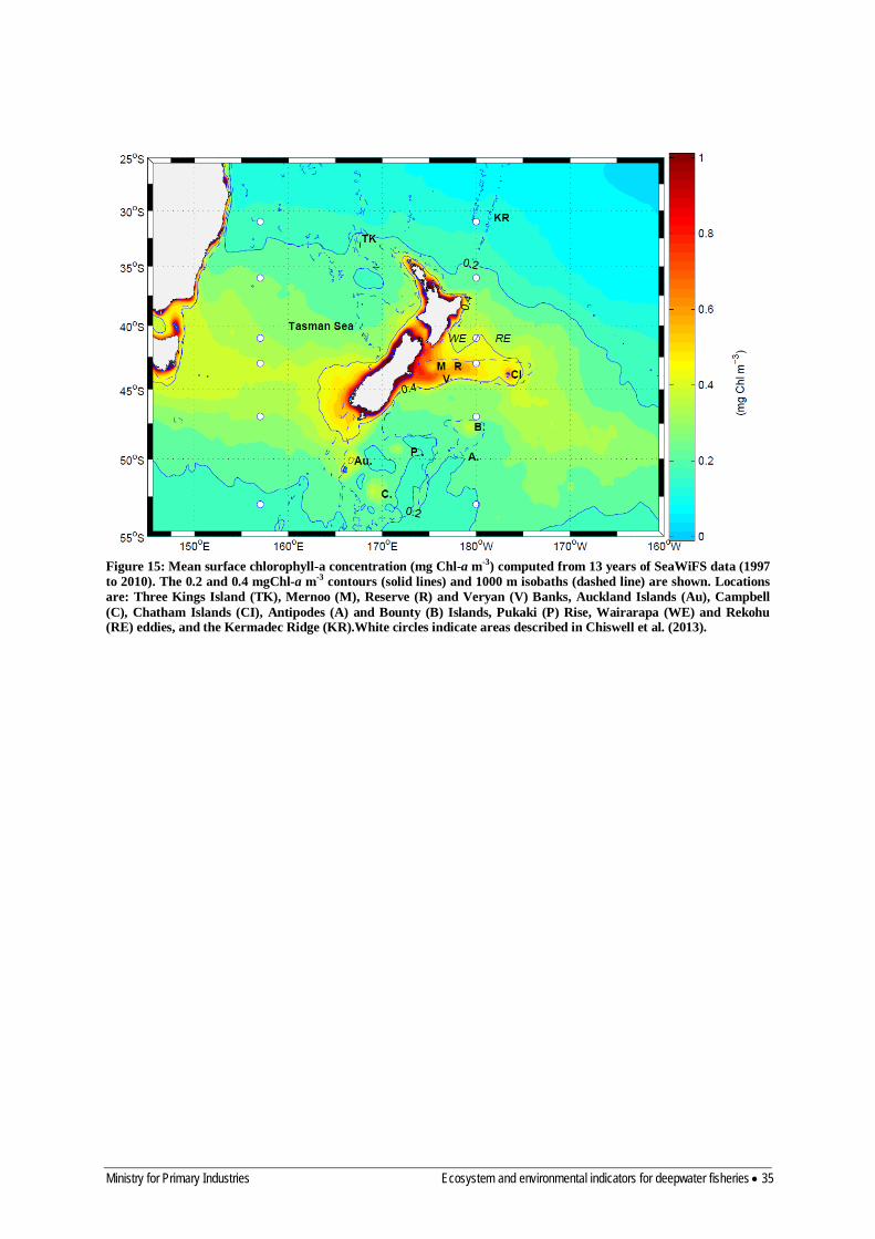
Ministry for Primary Industries Ecosystem and environmental indicators for deepwater fisheries • 35
Figure 15: Mean surface chlorophyll-a concentration (mg Chl-a m-3) computed from 13 years of SeaWiFS data (1997 to 2010). The 0.2 and 0.4 mgChl-a m-3 contours (solid lines) and 1000 m isobaths (dashed line) are shown. Locations are: Three Kings Island (TK), Mernoo (M), Reserve (R) and Veryan (V) Banks, Auckland Islands (Au), Campbell (C), Chatham Islands (CI), Antipodes (A) and Bounty (B) Islands, Pukaki (P) Rise, Wairarapa (WE) and Rekohu (RE) eddies, and the Kermadec Ridge (KR).White circles indicate areas described in Chiswell et al. (2013).
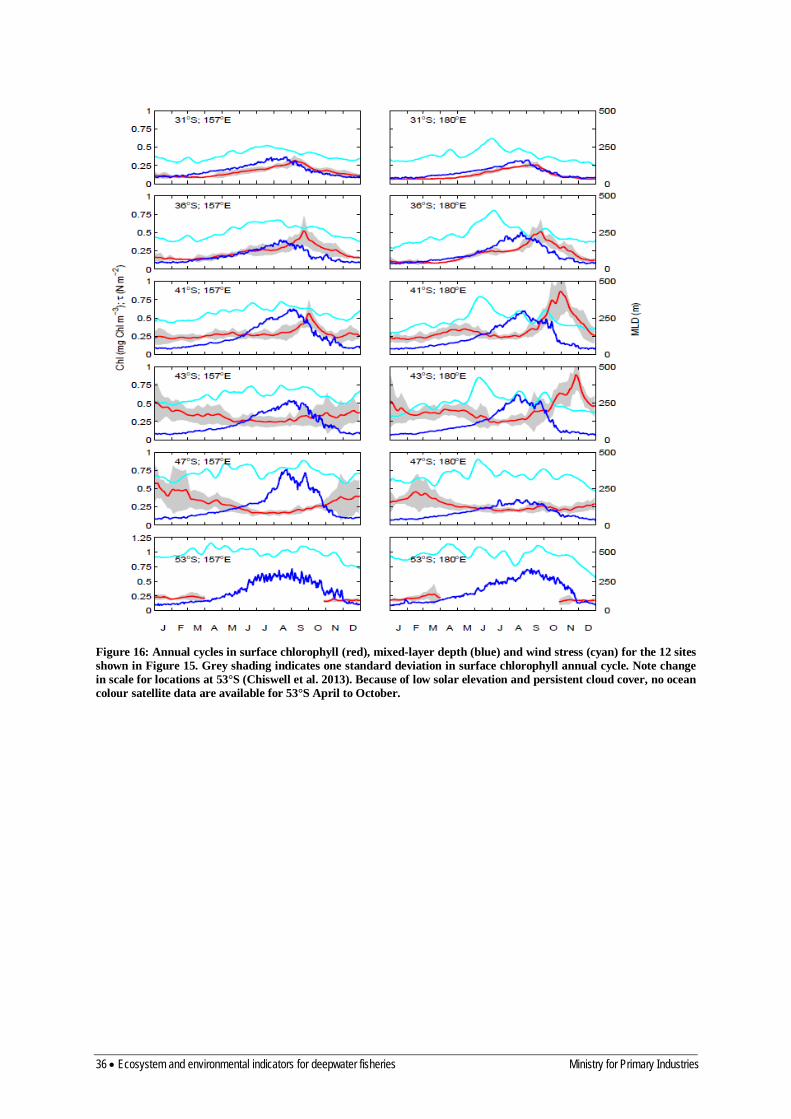
36 • Ecosystem and environmental indicators for deepwater fisheries Ministry for Primary Industries
Figure 16: Annual cycles in surface chlorophyll (red), mixed-layer depth (blue) and wind stress (cyan) for the 12 sites shown in Figure 15. Grey shading indicates one standard deviation in surface chlorophyll annual cycle. Note change in scale for locations at 53°S (Chiswell et al. 2013). Because of low solar elevation and persistent cloud cover, no ocean colour satellite data are available for 53°S April to October.

Ministry for Primary Industries Ecosystem and environmental indicators for deepwater fisheries • 37
Figure 17: The first two EOFs of surface chlorophyll annual cycles in the New Zealand region. (A) Spatial and temporal components of the first EOF; (B) Spatial and temporal components of the second EOF.
EOF analysis was also calculated for Chl-a (Figure 18). This analysis aims to bring out patterns of long-term change in the region. The first EOF explained 49% of the variance. The principal Chl-a EOF is plotted along with the Southern Oscillation Index (SOI) (plotted negative and scaled to have the same variance as the EOF for visual comparison, Figure 18). Note that these time series are far too short to compute formal correlations. The first Chl-a EOF shows a band of high amplitude west of New Zealand spanning the Tasman Sea. Its temporal component is approximately flat from 1998 until 2002 but then rises, with some fluctuations until 2009; there is very little apparent correlation with the SOI. This result implies that variations in primary productivity in the New Zealand ocean have complex drivers, so that monitoring of Chl-a patterns, in addition to climate indices, is likely to be useful for providing environmental context to changes in fisheries.

38 • Ecosystem and environmental indicators for deepwater fisheries Ministry for Primary Industries
Figure 18: The first EOF for surface chlorophyll-a anomalies in the New Zealand region (λ1=0.49). Top: Spatial component. Lower: Temporal component (solid blue line). The dashed line in the lower panel indicates the Southern Oscillation Index (SOI) which is plotted negative and scaled to have the same variance as the EOF for visual comparison.
5.1.5 Carbon-chlorophyll ratios for marine phytoplankton In order to estimate phytoplankton biomass in the upper ocean, it is necessary to convert Chl-a to carbon, and estimate the vertical distribution of phytoplankton through the water column. Carbon-chlorophyll ratios for marine phytoplankton have been found to vary considerably from 20 to over 200 gCg-1Chl-a (Taylor et al. 1997, Lefevre et al. 2003). Data from SOIREE (Boyd 2002) and other experiments in iron-limited waters suggest that a seasonally-invariate value of 80–100 gCg-1Chl-a for sub-Antarctic waters is reasonable. In New Zealand Subtropical waters, work suggests a seasonal variation in C:Chl-a values of approximately 50 gCg-1Chl-a before the spring bloom, 40 gCg-1Chl-a during the spring bloom, and 60 gCg-
1Chl-a after the bloom (Boyd 2002; Boyd unpublished data).
5.2 Primary productivity Photosynthesis is the process by which plants use the energy in sunlight to fix carbon dioxide (CO2) into organic material. Aquatic and terrestrial photosynthetic plants use some of their newly formed carbon products immediately for energy and maintenance. The remaining

Ministry for Primary Industries Ecosystem and environmental indicators for deepwater fisheries • 39
photosynthetic products are available for plant growth or consumption by the heterotrophic community. We refer to this “available” carbon as net primary production (NPP), and it is equal to gross photosynthetic carbon fixation minus the carbon respired to support maintenance requirements of the whole plant. NPP is measured as milligrams of organic carbon produced by photosynthesis per square metre per day (mgC m-2 d-1). Total net primary production on Earth exceeds 100 billion tons of carbon per year, and plays a profound role in the global carbon cycle. NPP by phytoplankton in the ocean provides virtually all the energy to fuel oceanic ecosystems, including fisheries, marine mammals and seabirds. As a general result, the secondary production of fishes (and by extension, the sustainable fisheries yield) in ecosystems tends to be positively related to the amount of primary production in the system, at least at large (basin) spatial and long (multi-annual) temporal scales (Pauly & Christensen 1995, Pikitch et al. 2004, Friedland et al. 2012).
5.2.1 Satellite-based methods of measuring NPP Light, temperature, and nutrient concentrations are major factors controlling phytoplankton growth rates, community structure, and primary production in the surface mixed layer of the ocean (Parson et al. 1977, Arrigo 2005). NPP can be measured accurately from ships (typically using radio-active carbon incubations), but because of the high spatial and temporal variability of NPP, ship-based sampling cannot adequately observe carrying capacity at scales appropriate to the size of the New Zealand EEZ. Instead, remotely-sensed data from Earth-observing satellite sensors are typically used to estimate NPP at basin scales. The original empirical models of NPP (e.g., Platt 1986) have been superseded by simple mechanistic models based on three factors:
• phytoplankton biomass, usually estimated via the proxy of chlorophyll-a concentration (Chl-a) obtained from ocean colour satellite sensors;
• average light intensity for phytoplankton, which is affected by the intensity of incident light at the sea-surface and the depth to which phytoplankton mix in the surface ocean. Light availability for phytoplankton is usually estimated using four interlinked models: (1) model of light at the sea surface (downwelling cosine irradiance at wavelengths between approximately 400 and 700 nm) using measurements of cloud reflectivity from ocean colour satellite sensors and a knowledge of solar and viewing geometry; (2) model of light penetration through wave-roughened sea surface; (3) effect of phytoplankton and other coloured material in the water column on downwelling light attenuation (the rate at which the intensity of light decreases with depth); (4) model of mixed layer depth (e.g. CSIRO Atlas of Regional Seas, CARS2000) (Dunn & Ridgway 2002);
• yield function which incorporates the physiological response of the phytoplankton to light, nutrients, temperature and other environmental variables such as temperature, macro and micronutrient availability, and phytoplankton photo-physiology (e.g. functional groups of phytoplankton present, adaptations to light availability). Phytoplankton physiology accounts for a large proportion (probably the majority) of variability in measured NPP in the ocean, but is poorly measured remotely and is likely to vary at relatively small time and space scales. In the absence of other information at appropriate scales, remotely-sensed sea surface temperature (SST) is often used to parameterise this yield function.
A range of such modelling approaches exist (e.g., Platt & Sathyendranath 1993, Longhurst et al. 1995, Antoine & Morel 1996a, 1996b, Behrenfeld & Falkowski 1997b, Howard & Yoder 1997, Ondrusek et al. 2001, Westberry et al. 2008). The various approaches are distinguished

40 • Ecosystem and environmental indicators for deepwater fisheries Ministry for Primary Industries
by the degree of integration over depth and irradiance, and the manner in which temperature is used to parameterise the photosynthetic yield function (Behrenfeld & Falkowski 1997a). One exception is a recent new approach to NPP modelling which is based on satellite-observed carbon rather than chlorophyll. This method takes advantage of recent developments in inherent optical property retrievals from ocean colour instruments, and the realisation that there might be important information on phytoplankton physiological state in these measurements (Behrenfeld et al. 2005, Westberry et al. 2008). However, this carbon-based method is unvalidated at present, and the more established methods based on Chl-a are generally still preferred for estimating NPP. There are significant quantitative differences (by a factor of more than 2) between all the various methods of estimating NPP (Campbell et al. 2002), and it is not yet known whether any of these satellite estimates of NPP bracket the true value in the New Zealand region (Schwartz et al. 2008). It is likely that most of the differences in NPP models are due to alternative approaches to handling variations in phytoplankton physiology. Results of applying three leading NPP algorithms to global satellite data are available from the Oregon State University “Ocean Productivity” project (web.science.oregonstate.edu/ ocean.productivity) at a spatial resolution of 10’ in latitude and longitude, which equates to resolution of approximately 18.6 km (latitude) and 12–16 km (longitude) for the New Zealand EEZ:
• Standard-Vertically Generalized Production Model algorithm (VGPM) (Behrenfeld & Falkowski 1997a) is a chlorophyll-based model that estimates NPP from chlorophyll using a temperature-dependent description of chlorophyll-specific photosynthetic efficiency. For the VGPM, net primary production is a function of chlorophyll, available light, and the photosynthetic efficiency.
• Eppley-VGPM algorithm: This model differs from the Standard VGPM only in the
use of an exponential temperature-dependent description of photosynthetic efficiencies (Eppley 1972). While Eppley’s analysis has no direct relationship to the description of average photosynthetic efficiencies, its application in ocean productivity models is commonplace. The exact “Eppley-function” used in the VGPM is based on the productivity model of (Morel 1991).
• Carbon-based Production Model (CbPM) (Behrenfeld et al. 2005, Westberry et al.
2008) is based on the observation that estimation of NPP using chlorophyll and temperature-based models rely on yield terms that are empirical descriptions of physiological variability, and often perform poorly when compared to local field measurements.
5.2.2 NPP estimates for the New Zealand region Variations between three leading approaches to estimating NPP from satellite data in the New Zealand EEZ are substantial (Figure 19), and it is not yet known whether these estimates bracket the true value (Schwartz et al. 2008). Although there are large differences between the estimates of NPP by the three main candidate algorithms, they all capture the strong annual seasonality in NPP around New Zealand. NPP peaks in the late-spring/early summer (December-January), and has an annual minimum in the late winter (July-August). The VGPM model suggests that the phase of NPP is about a month earlier than the CbPM and

Ministry for Primary Industries Ecosystem and environmental indicators for deepwater fisheries • 41
Eppley models show. NPP by the CbPM model has the largest dynamic range seasonally, and also the highest maximum values of NPP. The Eppley model has the smallest seasonal range, and also estimates the lowest maximum production values. The VGPM model gives almost the same maximum NPP values as CbPM, but significantly higher annual minimum values.
Figure 19: Average Net Primary Production (NPP) estimates for the New Zealand EEZ from three algorithms: Carbon-based Production Model (CbPM) (Behrenfeld et al. 2005, Westberry et al. 2008); Standard-Vertically Generalized Production Model algorithm (VGPM) (Behrenfeld & Falkowski 1997a); Eppley-VGPM algorithm (using Eppley 1972; see text). All results are based on MODIS-Aqua data ocean colour data.
None of the methods has been adequately validated in New Zealand waters (Schwartz et al. 2008) but work to date suggests that the standard VGPM-model (Behrenfeld & Falkowski 1997a) best fits the measurements made at sea. The standard-VGPM model has been used to investigate variability and trends in NPP over the New Zealand EEZ (Pinkerton 2007), and is shown in Figure 20 and Figure 21. This model uses SST to estimate availability of nitrate in the surface layer of the ocean; cooler waters tend to contain higher concentrations of nitrate in New Zealand waters, as elsewhere (Sherlock et al. 2007). Globally, higher concentrations of nitrate tend to lead to higher NPP, as phytoplankton growth in many oceanic waters is limited by nitrate availability (Dugdale & Goering 1967, Fanning 1989, Levitus et al. 1993). In New Zealand waters, this situation typically applies north of the Subtropical Front (STF). South of the STF, phytoplankton growth can be limited by a complex interaction of light, silicate and iron availability (Boyd et al. 1999, Murphy et al. 2001) – so-called “high-nitrate low chlorophyll” (HNLC) conditions. Global NPP methods are not expected to perform well under these conditions (Campbell et al. 2002, Carr et al. 2006). In the HNLC waters, it is likely that modelled values of production are towards the upper limit of possible values in sub-Antarctic waters (e.g., Moore & Abbott 2000).
0
100
200
300
400
500
600
1997 1999 2001 2003 2005 2007Date
NPP
(mgC
m-2
d-1
)
CbPMVGPMEppley
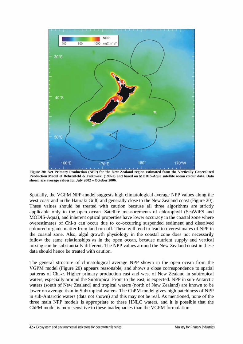
42 • Ecosystem and environmental indicators for deepwater fisheries Ministry for Primary Industries
Figure 20: Net Primary Production (NPP) for the New Zealand region estimated from the Vertically Generalized Production Model of Behrenfeld & Falkowski (1997a) and based on MODIS-Aqua satellite ocean colour data. Data shown are average values for July 2002 – October 2006.
Spatially, the VGPM NPP-model suggests high climatological average NPP values along the west coast and in the Hauraki Gulf, and generally close to the New Zealand coast (Figure 20). These values should be treated with caution because all three algorithms are strictly applicable only to the open ocean. Satellite measurements of chlorophyll (SeaWiFS and MODIS-Aqua), and inherent optical properties have lower accuracy in the coastal zone where overestimates of Chl-a can occur due to co-occurring suspended sediment and dissolved coloured organic matter from land run-off. These will tend to lead to overestimates of NPP in the coastal zone. Also, algal growth physiology in the coastal zone does not necessarily follow the same relationships as in the open ocean, because nutrient supply and vertical mixing can be substantially different. The NPP values around the New Zealand coast in these data should hence be treated with caution. The general structure of climatological average NPP shown in the open ocean from the VGPM model (Figure 20) appears reasonable, and shows a close correspondence to spatial patterns of Chl-a. Higher primary production east and west of New Zealand in subtropical waters, especially around the Subtropical Front to the east, is expected. NPP in sub-Antarctic waters (south of New Zealand) and tropical waters (north of New Zealand) are known to be lower on average than in Subtropical waters. The CbPM model gives high patchiness of NPP in sub-Antarctic waters (data not shown) and this may not be real. As mentioned, none of the three main NPP models is appropriate to these HNLC waters, and it is possible that the CbPM model is more sensitive to these inadequacies than the VGPM formulation.

Ministry for Primary Industries Ecosystem and environmental indicators for deepwater fisheries • 43
Figure 21: a: Average Net Primary Production (NPP) over the New Zealand region estimated from the Vertically Generalized Production Model of Behrenfeld & Falkowski (1997a) and based on two sets of satellite ocean colour data: blue, OrbImage Sea Viewing Wide Field-of-view Sensor (SeaWiFS); red, NASA Moderate Resolution Imaging Spectroradiometer (MODIS-Aqua). The effect of different ocean colour satellite data sources (SeaWiFS and MODIS-Aqua) is small at the New Zealand EEZ level. b: Change from the average monthly condition expressed as percentage of mean (%).
There is a suggestion of a small decrease in NPP in the New Zealand EEZ on average (1% y-1 based on SeaWiFS data, Figure 21). This is within the global envelope suggested by modelling studies (Sarmiento et al. 2004). Globally, satellite data suggest that annual NPP has declined by more than 6% since the early 80s (Gregg et al. 2003), though most of this decline (70%) occurred in high latitudes. The high interannual variability in the New Zealand data, lack of validation to date, and relatively short length of the time series means that these changes should be considered with caution. The changes are extremely unlikely to be affected by local New Zealand human activities, and more likely to be connected to variability in climate-related processes. Validating the satellite estimates of NPP, monitoring medium and long-term changes in NPP, and continuing to investigate the climate-ocean-ecosystem

44 • Ecosystem and environmental indicators for deepwater fisheries Ministry for Primary Industries
processes which may affect NPP, are important to determine whether the observed changes are genuine, to understand why the changes may be occurring, and to understand how the rest of the marine ecosystem may be affected by changes in NPP if genuine and sustained.
5.2.3 Effects of climate change on primary productivity Increased temperature of the upper layers of the ocean results in increased density stratification, which affects ocean productivity in two opposing ways. First, increased stratification suppresses upwelling of nutrients (nitrate primarily, but also phosphate, silicate and trace nutrients like iron) into the upper water column which will tend to lead to decreased production of phytoplankton. Second, at New Zealand latitudes, this decrease could be offset somewhat by a lengthened growing season because the mixed layer shallows earlier and deepens later in the year (Bopp et al. 2001) or because a shallower surface mixed layer results in phytoplankton receiving higher light levels on average. Where phytoplankton production is limited by the length of the growing season and/or light availability, shallowing of the mixed layer which lasts for more of the year could increase overall system productivity, provided that suitable macro- and micro-nutrients are available in surface waters. Overall, coupled physical/biogeochemical models predict a net decrease (about 5%) in global phytoplankton productivity under doubled CO2 conditions that increase oceanic thermal stratification and reduce upwelling of nutrients (Cox et al. 2000). However, because the factors affecting ocean primary productivity are complex and vary regionally, prediction of the effects of climate change on NPP in particular waters is difficult. Monitoring of these contrasting effects in the New Zealand region could be carried out using one or more of the following approaches: (1) estimate NPP using satellite algorithms based on remote measurements of ocean colour, incident light and sea-surface temperature (SST). For this approach to be useful, it will require that the methods used to estimate these variables, and the relationships between these factors and NPP hold under climate change conditions (e.g. the relationship between temperature, nutrient supply and phytoplankton ecology must not change substantially). Testing this constancy is likely to require periodic research voyages in the New Zealand region; (2) monitor change in chlorophyll-a concentration using ocean colour satellite measurements. This may be a more robust long-term monitoring tool for changes in ocean productivity in the New Zealand region as the satellite processing algorithms underlying the estimation of Chl-a in the upper ocean are likely to be more robust to changes in the bio-physical system than those for NPP. There is also some evidence that fisheries yields are more highly correlated with changes in Chl-a than in NPP (Friedland et al. 2012); (3) make long-term measurement of nutrients (especially nitrate) in the upper ocean. Recently, instruments have been developed for automated measurement of oceanic nitrate, for example, the ProPS-UV submersible UV process photometer (TRIOS, www.trios.de). Research is underway in New Zealand to test the efficacy of such sensors (Cliff Law, NIWA, pers. comm.). If measurement from this type of sensor are found to be robust and of the required accuracy, monitoring of upper ocean nutrients could be possible from ships of opportunity or other cost-effective platforms in the future; (4) monitor for changes in upper-ocean water column structure. Surface warming of the ocean combined with changes in ocean wind patterns may lead to changes in the upper ocean structure, and in particular, the shallowest depth at which density-stratification becomes

Ministry for Primary Industries Ecosystem and environmental indicators for deepwater fisheries • 45
persistent (mixed layer depth, MLD). Remote monitoring of MLD is not possible at present, but measurements may be carried out from research vessels (using CTD instruments) or ships-of-opportunity using expendable bathythermographs (Sutton et al. 2005). Modelling changes in MLD based on remotely-sensed forcing data (e.g. ocean winds, heat input) may be useful to understand possible change in NPP; (5) monitor light available to phytoplankton for primary production, as affected by cloud cover and seasonal changes in mixed layer depth. The former may be monitored using satellite ocean colour measurements (Frouin & Pinker 1995, Frouin et al. 2003a, Frouin et al. 2003b, Frouin & Murakami 2007, Su et al. 2007), and ongoing tracking of this could be a useful indicator of climatic forcing on the marine system.
5.3 Variation from baseline Satellite-based observations of NPP can be used to observe large scale changes in environmental conditions that may indicate regime shifts. Coupling this analysis with variations in SST, chlorophyll-a concentration and SSH is likely to increase the power of this approach for detecting large-scale oceanographic changes of relevance to fisheries management. Earth-observing satellite measurements of the New Zealand include sea-surface temperature (Uddstrom & Oien 1999), ocean colour (Murphy et al. 2001, Pinkerton et al. 2005), and sea-surface height (Laing et al. 1998). Relatively long time series of consistent information are now available from many of these remote observations: over 36 years for SST (1973–present), over 12 years for OC (1997–present), and over 17 years for SSH (1992–present). Statistical techniques such as rotated empirical orthogonality function analysis (EOF) and principal components have become standard methods for the extraction of characteristic spatio-temporal patterns from such time-series of meteorological and oceanographic measurements (Preisendorfer 1988, Emery & Thomson 1997). As has been carried out elsewhere (Polovina & Howell 2005), combined and/or separate EOF analyses of these satellite datasets should be used to provide an oceanographic baseline against which to develop an index of oceanographic change in the New Zealand EEZ, and also potentially act as an indicator of climate-driven regime shift (Brierley & Kingsford 2009). In addition, spatial maps of trends in Chl-a, primary production, SST, or other satellite observations of oceanographic state would be useful to identify “hotspots” of environmental change.
5.4 Recommended candidate indicators for Primary productivity Monitoring the base of the oceanic food-web (upper ocean phytoplankton) is likely to be both cost effective and relevant to deepwater fisheries, in that it provides an indication of potential changes to food-availability to the bathy-demersal zone. The available indicators of primary production include:
• Chlorophyll-a concentration • Incident irradiance (PAR) • Net primary production
Satellite observations of chlorophyll-a concentration in the New Zealand region are credible, available now, and include data from the present back to 1997. Such data are likely to be available for the next decade at least.

46 • Ecosystem and environmental indicators for deepwater fisheries Ministry for Primary Industries
Estimates of primary production (the rate of carbon fixation by marine phytoplankton) are available for the New Zealand region at present, but are considered less credible due to variations in the factors affecting phytoplankton growth in different regions. The relationship between incident light (PAR) and primary production is similarly complex, being affected by water column structure, nutrient availability and phytoplankton ecology.
6 FOOD-WEB INDICATORS
6.1 Trophic ecosystem services supporting fisheries Although the amount of organic matter fixed by phytoplankton (net primary production, NPP) places an upper limit on the carrying capacity of marine ecosystems (Pauly & Christensen 1995, Pikitch et al. 2004) there is significant complexity in the relationship between NPP and the abundance of predators like fish, shellfish, marine mammals, and seabirds that can be sustained in the long term (Figure 22). The consumption of fishes in ecosystems is a relatively small proportion (a few percent) of NPP, so that although the total amount of energy entering marine ecosystems certainly affects productivity at higher trophic levels, the pathways and overall efficiency by which energy is passed through ecosystems is crucial to the amount of high trophic level organisms (including fishes) that can be supported, and hence the level of sustainable fisheries yield. All but a tiny fraction of primary production in oceanic ecosystems occurs in the upper mixed layer (generally less than 100 m deep). However, most food consumed by commercially-important fishes (particularly for the deepwater ecosystem considered here) occurs at depth, either in the mesopelagic zone or near the sea-bed (below the surface mixed layer). Organic matter produced by phytoplankton is also too dispersed to be directly consumed by higher predators such as fishes. Instead, a range of organisms link phytoplankton to higher predators through the ocean food-web, and act to “repackage” organic matter into forms that are consumed by higher trophic level species. Friedland et al. (2012) examined the relationships between NPP, fisheries yields, and parameters describing the transfer of organic matter through 52 large marine ecosystems (in this analysis, the New Zealand area is a single “large marine ecosystem”). They found that chlorophyll concentration, the particle-export ratio (the proportion of NPP exported from the surface layer of the ocean, p-ratio) and the ratio of mesozooplankton productivity to NPP (z-ratio) were significantly related to fisheries yields. Stock & Dunne (2010) suggest that a warmer ocean will lead to a lower z-ratio (less mesozooplankton for a given NPP) and Friedland et al. (2012) show that lower z-ratios correspond to lower fisheries yields at basin scales. Indicators for the p-ratio and z-ratio may hence be useful indices of ecosystem change that may affect fisheries productivity.

Ministry for Primary Industries Ecosystem and environmental indicators for deepwater fisheries • 47
Figure 22: Simplified trophic model of the Chatham Rise, New Zealand (based on precursor to Pinkerton 2011). The growth of phytoplankton generates organic matter that is the fuel for the marine ecosystem. Figures show the annual flow of energy through unit area of the food-web normalised to an NPP=100, based on an equilibrium mass-balance model (similar to Ecopath).
6.2 Prey species for commercially-important fish Feeding studies on commercially-important fishes in the New Zealand Quota Management System show that small midwater fishes (especially myctophids, javelinfish), meso- and macro-sized crustacean zooplankton, gelatinous zooplankton (especially salps), cephalopods, and hyperbenthic crustaceans (especially shrimps and prawns) are crucial prey items (Clark 1985, Clark et al. 1989, Dunn et al. 2009a) (Table 1). Some fish feed on truly benthic epifauna or infauna, like nematodes in the soft sediments, but most commercially-important fishes in New Zealand waters feed on middle-trophic level mesopelagic and hyperbenthic species. Mesopelagic prey animals (those living in the midwater), include meso- and macro-zooplankton (especially crustacean zooplankton like krill and copepods), gelatinous zooplankton (salps, jellyfish), cephalopods (squids, octopods), larval and juvenile fish (ichthyoplankton), and “bait-fishes” (including more than 21 species of myctophids: McClatchie et al. 2005, O'Driscoll et al. 2009). The other main group of middle-trophic level biota are hyperbenthic animals - those living close to the sea-bed. These include decapods (especially Munida gracilis [squat lobster] and Metanephrops challenger [scampi], Pasiphaeid and Pandallid shrimps), amphipods and polychaetes. The key role of these middle-trophic level species in ocean ecology is well known (e.g., Marine Zooplankton
48 • Ecosystem and environmental indicators for deepwater fisheries Ministry for Primary Industries
Colloquium 2, 2001; Banse 1995, Smetacek et al. 2004), but they have been under-studied in New Zealand. Middle trophic level “linking” organisms have varied energetics and life histories which affect the number and type of predators that can be supported by a given amount of NPP. These species are likely to be affected both by fishing reducing top-down predation control, and by climate-driven changes in lower trophic food-web components (Frank et al. 2007, Richardson 2008). Developing indicators for these prey species may be useful and important. The studies listed below (Table 1) are based on samples collected during trawl surveys, although observer sampling at sea identification of stomach contents by observers have also provided valuable information for some species (Horn et al. 2013c). Table 1: Selected diet studies of some New Zealand deepwater fishes.
Species References Hoki Connell et al. (2010) Ling, hake Dunn et al. (2010a) Orange roughy Rosecchi et al. (1998); NIWA unpublished data (Coasts & Oceans
Programme 2) Oreo (black, smooth) Clark et al. (1989) Alfonsino Horn et al. (2010) Chimaeroid fishes Dunn et al. (2010b) Warehou (silver, white) Horn et al. (2011) Red cod, sea perch Horn et al. (2012) Southern Ray’s Bream Horn et al. (2013b) Orange perch Horn et al. (2013a) Macrouridae Stevens and Dunn (2011); Stevens (2012) Squaliforme sharks Dunn et al. (2013)
6.3 Bentho-pelagic coupling The fact that the main prey species of deepwater fishes have a benthic or hyperbenthic (on the seabed, or within a few metres above it) association, means that coupling between the surface ocean and depth is important to the efficiency by which energy is transferred from primary producers to fishes. These prey species are typically small-sized bottom-dependent animals that have good swimming ability and perform, with varying amplitude, intensity and regularity, seasonal or daily vertical migrations above the seabed. Three processes are important to the bentho-pelagic coupling, and hence the level of sustainable fisheries yields: (1) the proportion of NPP that is exported from the surface mixed layer (particle-export ratio); (2) the proportion of downward organic flux through the base of the mixed-layer that reaches the sea-bed (which depends sinking rates, the speed of bacterial degradation of sinking material, and the types of organism living in the water columns and near the sea bed which feed on sinking detritus); (3) the diel movement cycles of deepwater fishes and other biota. The proportion of NPP exiting the base of the surface mixed layer is called the particle export ratio (p-ratio), and empirical and semi-empirical models exist to predict this value based on, inter alia, sea surface temperature (SST) and NPP (Dunne et al. 2005, Buesseler & Boyd 2009). The processes affecting the flux of organic matter to the sea-bed may be affected by climatic and environmental forcing. In oceanic systems like those of New Zealand, about 30–50% of NPP is likely to exit the base of the surface high productivity layer. Models suggest that SST is the most important factor affecting the p-ratio, and that ocean warming will lead

Ministry for Primary Industries Ecosystem and environmental indicators for deepwater fisheries • 49
to a lower proportion of NPP being exported to depth, with a corresponding reduction in fisheries yield (Friedland et al. 2012). Organic matter sinking through the water column is consumed by microbial and meso/macro-sized organisms in the water column (Buesseler et al. 2007, Boyd 2008). These mesopelagic organisms “repackage” the detrital material, making it possible for fishes to feed off the sea-bed and also affecting the amount of material reaching the sea-bed. Only a small proportion of material (5–10% of NPP) reaches the sea-bed as passively-sinking particles. Recent research using the metabolic theory of ecology suggests that individual metabolic rates, growth, and turnover rates of benthic biota are directly related to bottom water temperature, but that higher-order community structure and function is affected by chemical energy limits (McClain et al. 2012), i.e. that the amount of material reaching the sea-bed ultimately affects the type of benthic and deepwater communities that occur there. In addition, there will be active bentho-pelagic coupling, whereby organisms migrate from the sea-bed into the water column where they consume food, and then migrate to the seabed taking the consumed material with them, but the magnitude of this transfer is poorly known.
6.4 Indicators for middle trophic level organisms Biodiversity has long been hypothesized to be a major determinant of ecosystem stability (e.g., Odum & Odum 1953, McCann 2000, Hooper et al. 2005). Perry et al. (2010) characterise unexploited marine ecosystems as having relatively large abundances of high trophic level species (like large deepwater fishes) supported by several mid-trophic level species with an uneven mixture of large and small abundances. Perry et al. (2010) suggest that the reduction in the abundance of high trophic level species by fisheries exploitation may simplify the mid-trophic level organisms to a smaller number of species but with larger and more even abundances. This simplification may lead to marine ecosystems which track variability in oceanographic conditions more closely and hence are less resilient to climate-driven change (Perry et al. 2010). Indicators that monitor change in the biodiversity (especially evenness of abundance) of the middle trophic level would hence be useful, as increasing evenness or reducing biodiversity of middle trophic level biota would indicate reducing resilience to climate variability and change. Few data exist for middle trophic level organisms in the New Zealand deepwater marine ecosystem, and we cannot as yet monitor their state. Three promising approaches may be useful in due course. First, New Zealand acquired a Continuous Plankton Recorder (CPR) in 2008 and this has been deployed twice to date as a start of a time series of zooplankton monitoring over the Chatham Rise. In other parts of the world, long time-series of measurements of the zooplankton community by the Continuous Plankton Recorder (CPR) have demonstrated regime shifts (Aebischer et al. 1990, Beaugrand et al. 2002), and been recommended as an effective way of monitoring the state of pelagic ecosystems (Beaugrand 2005). In due course these data could provide an indicator of change in the zooplankton community in the New Zealand upper ocean. The limitations of this approach are that: (1) it is focussed on the near-surface layer and gives no information on organisms deeper in the water column; (2) it is limited to small zooplankton, and does not sample middle-sized prey organisms like myctophids and decapods. Second, research is underway to investigate whether multifrequency acoustic backscatter data taken from research vessels during the annual surveys of fish on the Chatham Rise and Southern Plateau can be used to derive indices of abundance of mesopelagic fish and krill in

50 • Ecosystem and environmental indicators for deepwater fisheries Ministry for Primary Industries
these regions (O’Driscoll pers. comm.). Such data could be collected from appropriate echo sounders at minimal cost. Results from the analysis of the New Zealand survey data are not available at present, although the method has been applied successfully elsewhere (Trenkel & Berger 2013). It is likely that the method will not be able to resolve mesopelagic biota to species or genus (O’Driscoll pers. comm.), but rather, give an indication of biomass at the “mesopelagic fish versus krill” level. Even this level of discrimination would provide a useful indicator of the mesopelagic community size and structure, providing valuable data on this important prey resource, calculated from data already being collected. However, acoustic methods such as these give little information on changes to the abundance of hyperbenthic crustaceans such as decapods. Third, ongoing monitoring of stomach contents of key deepwater fishes may provide information on changes in the mesopelagic or hyperbenthic community. Diet may not necessarily reflect prey availability (Pinnegar et al. 2003), but changes in diet should reflect changes in the prey community. Horn & Dunn (2010) examined the diet of hoki, hake or ling from stomach contents analysis of specimens taken from the Chatham Rise between 1990 and 2009. Although the results of this analysis were inconclusive, the method may provide a cost-effective way of monitoring for change in the middle-trophic level community.
6.5 Recommended candidate indicators for Food webs Understanding change in deepwater fish communities that arises from environmental/ecosystem forcing will require indicators of key components of the food-web to be available. Potential indicators likely to be most useful include:
• Mesopelagic fish biomass • Crustacean zooplankton biomass and distribution • Gelatinous zooplankton biomass and distribution • Mesopelagic fish community • Mesopelagic plankton community from CPR
The development of methods to estimate the biomass of key mesopelagic prey species from multifrequency acoustics run opportunistically on trawl surveys provides the potential to obtain this information cost-effectively. More detailed examination of changes in the mesopelagic fish community may require dedicated midwater trawling, although indications of changes in community composition may also be apparent from stomach sampling of key fish predators. Establishing a regular survey of the upper ocean zooplankton community in a key area (such as the Chatham Rise) would provide potentially important information to monitor for changes in community structure that may be relevant to deepwater fisheries. Deployment of the Continuous Plankton Recorder from a ship of opportunity would be the most feasible way of acquiring this kind of zooplankton community data.
Ministry for Primary Industries Ecosystem and environmental indicators for deepwater fisheries • 51
7 FISHERIES AND FISHERIES MANAGEMENT INDICATORS
7.1 Fishing pressure indicators A range of indicators associated with fishing activities are available in the literature, and can be divided into those related to removals, fishing effort (particularly in relation to benthic disturbance), and management activity.
7.1.1 Fishing removals Total fishing removals gives a very clear indication of the pressure of fishing on the marine environment, and is a key OECD pressure indicator (OECD 2008). Where available, estimates of fishing mortality provide an ideal species level indicator, although these are generally limited to the more commercially important species, with accepted stock assessments. Catch can be broken down into species (or species group), fishery or regional level (Freon et al. 2005), or fate (i.e., discard rate). Total landings can be used in conjunction with biomass estimates (from assessments or surveys) to generate indicators such as inverse fishing pressure (1/(landings / biomass)) (Shin et al. 2010), or species catches can be expressed as a proportion of sustainable yield (Gilbert et al. 2000). Catch data disaggregated by species can also be used to generate other indicators related to commercial catch composition, but as discussed above in relation to TL, it must be remembered these are likely to be sensitive to market driven fishery targeting decisions (Branch et al. 2010, Pinkerton 2010), and may not reliably measure ecosystem level parameters. Indicators like the mean depth of catches or the mean distance from the coast have been used to track the development of fisheries from shallow coastal to deeper offshore areas (Freon et al. 2005), although this may not be particularly relevant when specifically examining deepwater fisheries. Illegal, unreported and unregulated (IUU) fishing is by definition unreported, and is therefore difficult to quantify. However, there may be enforcement agency estimates of IUU catches for some fisheries available, which could be expressed as a proportion of total catches as an indicator, or records of IUU convictions, that may reflect both the pressure put on fisheries by IUU fishing, and the level of management response. In addition to total fishery removals acting as a pressure on the ecosystem, species specific fishery related removals (particularly those considered to be endangered) may be considered a useful indicator, and are routinely monitored for New Zealand fisheries (Thompson & Abraham 2010). These are considered in Section 10, along with other indicators related to these species.
7.1.2 Fishing effort Bottom trawling is pervasive throughout much of New Zealand’s EEZ shallower than about 1200 m, and is probably the predominant disturbance agent deeper than about 100 m (Cryer et al. 2002). With the development of vessel monitoring systems (VMS) in the mid to late 1990s and early 2000s in many regions of the world, largely to address compliance issues, and improved scientific access to the data, fisheries scientists have been able to map patterns of fishing effort at far finer scales of resolution than ever before (Lee et al. 2010, Jennings et al. 2012), although often landings are still recorded on a daily basis, introducing difficulties in allocating catches to individual trawl tracks (Gerritsen & Lordan 2011). Although New Zealand has been running a VMS since 1994, the Trawl Catch Effort Processing Return

52 • Ecosystem and environmental indicators for deepwater fisheries Ministry for Primary Industries
(TCEPR) system, recording trawl positions (start and finish locations) and main catch components on an individual tow basis, has been used by vessels trawling in deepwater areas since the 1989–1990 fishing year. This provides a very valuable source of information on spatial and temporal patterns of trawl fishing effort, and Baird et al. (2011) provide a comprehensive review of data collected from 1989–90 to 2004–05, describing fishing patterns through measures of fishing intensity or coverage (Figure 23). More recent examination of the data has focussed on coverage (footprint) rather than intensity (Black et al. 2013), but both approaches provide valuable insight into fishing patterns and pressure on seabed habitats (e.g., BOMEC class). Some fisheries have only recently (since October 2007) started recording trawl positions (start position only) within the Trawl Catch Effort (TCE) system, but these are generally focussed in inshore areas. Piet et al. (2007) examined a range of potential fishing effort related indicators, and found that indicators at increasing levels of detail (going from number of vessels at the low detail end; to overall effort; to fishing intensity; to fishing mortality at the high detail end) differed considerably in their description of present and historical fishing impact. Many of the patterns identified in the fishing mortality data, representing the actual pressure on the ecosystem and its components, were not identified with the less detailed indicators, and the authors recommended using the highest level indicator that can be obtained with available data. For New Zealand deepwater assessed species, this highest level indicator would be some measure of fishing mortality (at the stock level), while for the remainder of the species, and habitats, fishing intensity (frequency of fishing, at fine spatial scales) would be the highest level indicator. Freon et al. (2005) developed indicators examining ratio of fished area to area of species distribution, and also the exploited proportion of an ecosystem’s spatial area. An index of collocation has been used to compare the distributions of different fish species, and would be equally applicable to compare fish and fishery distributions (Woillez et al. 2009a).
Figure 23: Left plot, distribution of aggregate swept area totals per cell, for trawl effort on or near the seafloor, based on TCEPR records, for the years 1989–90 to 2004–05 (Baird et al. 2011). Right plot, trawl footprint for the years 1989–90 to 2004–05 overlaid on the 15 level BOMEC (Baird et al. 2011).

Ministry for Primary Industries Ecosystem and environmental indicators for deepwater fisheries • 53
While bottom trawling is the fishing method most widely considered in relation to the effects of fishing (and has been the focus of most studies), bottom longline gear also has an impact on the benthic organisms (Munoz et al. 2010), with some taxa considered to be particularly vulnerable (Parker & Bowden 2010). Set net fisheries do not operate off the continental shelf, but gear deployed in shallower waters may potentially be swept into deeper areas. Similar fishing effort indices to those described above would also be relevant to these gears. Ghost fishing has been defined as the ability of fishing gear to continue fishing after all control of that gear has been lost by the fisher (Matsuoka et al. 2005), and is a component of IUU fishing. Ghost fishing by lost fishing gear has been examined for a range of gear types (Kaiser et al. 1996, Matsuoka et al. 2005, Adey et al. 2008), although research has generally focussed on lost trawls, traps and entangling nets. The consequences of gear loss depend on gear type and seabed conditions, but traps and entangling nets have been found to have the greatest potential impact, with some gears having been found to continue catching months after loss. Indicators of lost gear (either reported lost, or recovered) could be developed,
7.2 Fisheries Management Response Indicators Response indicators measure institutional propensity and capability for furthering sustainability of marine ecosystems (OECD 2003), and are an important part of a suite of indicators for measuring national progress towards sustainability. Important aspects of response include the current state of the scientific knowledge base needed to manage human impacts, the resourcing available to develop underpinning and applied knowledge, and an evaluation of what actions and systems are in place (or lacking) to promote sustainability.
7.2.1 State of fisheries knowledge The quality of information and state of knowledge on the status of fish stocks relative to management targets is an important measure of institutional progress towards the sustainable use of marine resources, and has previously been proposed for inclusion in New Zealand state of the environment reporting (Gilbert et al. 2000). The state of fisheries knowledge can be considered a measure of the level of investment in research relevant to fisheries management. Indicators could include the number of stocks for which there are accepted assessments, the proportion of the total landings from stocks with accepted assessments, or the proportion of catches from different fisheries from observed trips.
7.2.2 Bioregions protected indicator Indices showing the amount of fishable (largely dictated by depth) area closed to fishing are relevant to monitoring fishing pressure in the New Zealand region, and the percentage of marine environments/habitats under protection was proposed as an indicator for New Zealand by Gilbert at al. (2000). New Zealand’s approaches to defining habitats relevant to deepwater fisheries are described below. Offshore marine protection has been established in three phases. In 1990, an area of 7280 km2 around the Kermadec Islands was protected, and in 1997 a further 4980 km2 around the Auckland Islands was protected. In November 2007 17 Benthic Protection Areas (BPAs), with a total area of about 1.2 million km2, were closed to bottom fishing methods, namely bottom trawling and dredging, in perpetuity [Fisheries (Benthic Protection Areas) Regulations 2007].
54 • Ecosystem and environmental indicators for deepwater fisheries Ministry for Primary Industries
Spatial maps indicating where communities are predicted to be ecologically distinct are available from a number of New Zealand classification schemes, namely the Marine Environment Classification (MEC)(Snelder et al. 2004, Snelder et al. 2006), the Demersal Fish Classification (DFC)(Leathwick et al. 2006a, Leathwick et al. 2006b), and the Benthic Optimised MEC (BOMEC)(Baird 2009, Leathwick et al. 2012). The MEC covers the whole New Zealand EEZ, whereas the other two classification schemes only cover part of it. Of the area within the BPAs, 75% is deeper than 1950 m and not covered by the DFC, and 52% is deeper than 3000 m and not covered by BOMEC. In regions where MEC overlaps with the BOMEC and DFC (i.e. depths less than 1950 m), the MEC is known to offer much poorer separation of regions that are distinct in terms of their demersal fish than the DFC (Sharp et al. 2007), and poorer separation of regions that are distinct in terms of their demersal fish and benthic invertebrate assemblages than BOMEC (Leathwick et al. 2012). To a large extent, BOMEC encompasses and extends DFC by adding eight classes of benthic invertebrates to the 126 species of demersal fish (Leathwick et al. 2012). Ecologically distinct regions are called “bioregions”, and BOMEC provides the best bioregionalisation available for the New Zealand EEZ, although there are also specific deepwater habitat classifications which cover the New Zealand region (Rowden et al. 2005, Clark et al. 2011). The location of New Zealand’s BPAs are shown in relation to the 15 level BOMEC in Figure 24. The proportion of each New Zealand bioregion at fishable depths which is protected could be summarised as an indicator of management response. Combining the proportion of each bioregion protected into a composite index requires information on the relative ecological importance of the bioregions, and the protection-benefit trade-off curve i.e. how much additional conservation benefit is obtained from increasing amounts of area being protected. Information on this does not yet exist.

Ministry for Primary Industries Ecosystem and environmental indicators for deepwater fisheries • 55
Figure 24: New Zealand Benthic Protection Areas (BPAs) overlaid on the 15 level BOMEC.
7.2.3 Fisheries management indicators The indicators available to measure fisheries management activity and success vary with the levels of complexity of the management and assessment system. At a very basic level, the number of stocks with quota, and total expenditure on fish stock monitoring have been proposed as indicators of fisheries management (OECD 2008). Where stock assessments are conducted, a range of further indicators are available relating TACC to estimated sustainable yield (Gilbert et al. 2000), or actual catches to TACC. Aggregated across species, indicators summarising percentage of stocks with current biomass below target (or some other measure)(Gilbert et al. 2000), or percentage of stocks by exploitation level (under/moderately exploited, fully exploited, overexploited, depleted/recovering)(OECD 2008) have also been proposed, and a simplified version of this type of indicator is already provided annually for New Zealand (Ministry for Primary Industries 2013). In addition to national fisheries management approaches, international schemes (e.g. Marine Stewardship Council accreditation) are also reviewing fishery sustainability (largely for consumer chains), and the proportion of catches certified by such international schemes provides an indicator of how New Zealand’s fisheries are viewed globally. Another international measure would be the number of species in IUCN (or alternative) threatened categories (Gilbert et al. 2000). The proportion of total fisheries catches from the New Zealand EEZ that are from species which are not included in the New Zealand Quota Management System (QMS) would give an indication of the degree to which the New Zealand QMS encompasses the catch by New
56 • Ecosystem and environmental indicators for deepwater fisheries Ministry for Primary Industries
Zealand fisheries. There is likely to be less control of fishing mortality of species not included in the QMS compared to those included in the QMS, where catch is limited by an annual TAC limit, and hence less ability to quantify the risk to these species. This indicator is similar to a previously proposed indicator (ME31; Gilbert et al. 2000, OECD 2008). At present, catches of non-QMS species are not systematically recorded, except by fisheries observers. Consequently, although important, there is not likely to be a way to produce a useful indicator for this issue unless more details of catch composition (of non-QMS species) were routinely recorded by fishers. This would not be an insignificant task, and taxonomic identification issues could limit the utility of the data.
7.3 Recommended candidate indicators for Fisheries and Fisheries management Fishery activities are the main pressure on the marine ecosystem considered within the report, while management activities represent New Zealand society’s response to the effects of this pressure. The indicators considered to be most useful in relation to deepwater fisheries, covering the aspects related to fisheries activity and fisheries management are: Removals – providing a measure of the pressure exerted by fishing on the marine environment:
• Total removals (nationally, and by region or target fishery) • Inverse fishing pressure (1/(landings/biomass)) (by region)
Effort – providing a measure of the disturbance to benthic communities and habitats:
• Fishing footprint (by gear type, fishery and year, in relation to seabed habitat (BOMEC class, or other habitat classification))
• Fishing intensity (by gear type, fishery and year, in relation to seabed habitat (BOMEC class, or other habitat classification)).
Management activity and success – providing a measure of the investment in and success of the fisheries management system:
• Proportion of landings within the management system (QMS) • Observer coverage (proportion of trips and catches observed, by fishery and region) • Proportion of assessed stocks • Proportion of stocks by level of exploitation • Coverage of protected areas • Proportion of catches certified by international schemes
8 DEEPWATER FISH COMMUNITY INDICATORS Research associated with fisheries assessments mean that fish (and the invertebrates caught with them) communities are probably the most widely studied components of the marine ecosystem, with commercial landings and standardised research surveys providing the main data sources. Standardised trawl surveys are generally considered the best method for sampling biological indicators for a stock (assuming catchability is reasonably constant for a

Ministry for Primary Industries Ecosystem and environmental indicators for deepwater fisheries • 57
species over time and space, through careful standardisation of gear and fishing method) (Cotter et al. 2009). Commercial catch data (and how they relate to sustainable levels of fishing, where known) are considered within the fishing section (Section 7), and as they are dependent on fishing practice decisions, do not necessarily reflect the state of fish communities. The indicators discussed here relate to data available from trawl surveys. Trawl surveys provide standardised information on abundance, distribution, size frequency, and mean weight of the available fish community, and although the intention is that catchability remains relatively constant over time for a particular species, it may vary between species. Indicators developed from trawl survey data have been categorised into sections related to targeted species (often the part of the foodweb of most interest to humans), diversity, community composition, size composition, and trophodynamics (Fulton et al. 2005, Rochet & Rice 2005, Shin et al. 2010). A large number of studies have applied various indicators to trawl survey data, largely focussing on the whole sampled fish community rather than individual species, but relatively few have specifically examined deepwater fish communities (Tuck et al. 2009, Campbell et al. 2011). A recent European Union funded project FISBOAT on Fishery Independent Survey Based Operational Assessment Tools (FP6 contract No. 502572; www.ifremer.fr/drecohal/fisboat) has focussed more on single species indicators (Petitgas et al. 2009).
8.1 Exploited fish (targeted species) The focus of fisheries management to date has been on the exploited species, and a range of indicators have been developed describing different aspects of the abundance and distribution, size composition, and condition or reproduction of stocks. While discussed in relation to a population here, many of these indicators are equally applicable (and potentially more robust) across the whole sampled fish community. Trawl surveys routinely estimate abundance indices, usually by length or age class, and also total weight by species. Indicators based on these abundance data, relating to population growth rate and mortality, may be valuable when assessing species without accepted analytical assessments, although intrinsic growth rate (over the whole age structure) is likely to be sensitive to recruitment fluctuations, and so should be examined in conjunction with indicators that would identify these (Cotter et al. 2009). Weight per unit effort is less sensitive to fluctuations in recruitment than abundance or raw length indices (e.g., mean or median size), but changes in condition (weight/length) may be important. Numbers at length or age can reveal recruitment, relative year class strength and growth when monitored over time. They can be useful in interpreting changes in intrinsic growth rate, and have also been found to change rapidly in response to the initial fishing pressure when a fishery first develops (Jennings 2007), with numbers of older, larger individuals being reduced, and subsequently remaining low. Age data are not routinely collected for many species however, and precision can be an issue for some species, and so length based indicators are more commonly used. A range of descriptive statistics for length distributions (mean, median, quantiles, etc.) have been considered, with the median and L95 most commonly applied. The proportion of a stock that are juveniles (defined by size or maturity

58 • Ecosystem and environmental indicators for deepwater fisheries Ministry for Primary Industries
state) has been also used as an indicator (Hilborn & Walters 1992). Cumulative frequency plots of fish length have been examined for individuals and species groups (target, non-commercial, elasmobranchs) in comparing fish populations around Britain (Rogers & Ellis 2000), where marked reductions in the proportion of larger fish were observed. Size composition indicators are also discussed below. Indicators of reproductive capacity can give information on future sustainability of a stock. Spawning stock biomass (SSB) (and number; SSN) can be estimated if maturity at length or age is recorded. SSN is likely to track changes in age (or length) structure in populations, but can be informative when examined in conjunction with SSB and age structure, as large old fish are generally considered to be more successful spawners than young fish. If individual fish length and weight are routinely recorded on surveys, then these data can be used to calculate a fish condition index. Fulton’s condition index provides a measure of individual fish condition, and reflects overall habitat quality for growth and reproduction (Winters & Wheeler 1994). The gonadosomatic index (GSI) relates gonad weight to body weight, and can indicate nutritional state and reproductive fitness, but requires individual fish and gonad weights to be recorded, and can be sensitive to the timing of the spawning cycle. Mean length (or age) at maturity in a population is required to estimate the spawning indices above, and has been found to reduce under the effects of fishing, but may also vary geographically (Trippel 1995). A set of eight abundance, size, weight, sex ratio and reproductive parameters have been combined and analysed using univariate and multivariate techniques, to investigate changes over time for individual species (Ragonese et al. 2005). The multivariate analysis (multi-dimensional scaling of distance matrices) provided a more powerful approach to detect changes over time than examination of individual parameters, but the range of parameters combined for each species were far more extensive than those routinely collected on trawl surveys. Species distribution metrics describe the geographic locations of occurrences of a species. Species may exhibit range contractions as abundance decreases (although climate change may also have similar effects). Species distribution may be sensitive to spatial differences in the size structure of populations, combined with catchability. While spatial aspects of populations have not been widely used as an indicator, the percentage area of the survey within which x% (typically 90%) of the population occurs has probably been used most frequently (Swain & Sinclair 1993, Fisher & Frank 2004, Tuck et al. 2009) (Figure 25). More recently, Woillez et al. (2007, 2009a) have applied and reviewed a range of indicators describing and summarising the location, occupation of space, dispersion and microstructure of populations using fish density data collected during surveys. Other spatial indicators relating to species distribution and fishing patterns are described above (Section 7). Spatial behaviour of fishers has also been used to provide information on the spatial organisation of fish (Bertrand et al. 2005), on the basis that fisheries follow the distribution of fish. Spatial indicators vary with fish age and season (Woillez et al. 2007), but are likely to be useful in identifying changes in distribution over time. Petitgas & Poulard (2009) describe a multivariate approach to investigate spatial patterns in age-structured fish populations.

Ministry for Primary Industries Ecosystem and environmental indicators for deepwater fisheries • 59
Figure 25: Plots of the percentage of the Chatham Rise survey area over which 90% of the abundance (by weight) was distributed for the 25 most frequently caught species. Solid line (where shown) representing a significant linear fit through series (Tuck unpublished obs).
As the spatial distribution of unexploited populations is generally unknown, reference points for spatial indicators can only be determined by examining their evolution over time (Woillez et al. 2009b).
8.2 Diversity Measures of diversity are widely used in community ecology, with a variety of methods available. Diversity measures are a joint construct of how many species are present (richness), and how similar their abundances are (evenness), with some indices giving additional emphasis to the most abundant species in a community (dominance). However, there is concern that some of these measures may have little biological meaning (Fulton et al. 2004), that the relative weighting of richness and evenness used is often poorly justified (Rochet & Trenkel 2003), and that they may be misleading (Rice 2000), potentially missing regime shifts or guild replacements, and giving “false alarms” related to recruitment pulses. Measures of taxonomic diversity have been developed to address issues of relatedness
1995 2005
0.55
0.65
0.75
Year
90%
dis
trib
HOK
1995 2005
0.4
0.6
0.8
Year
90%
dis
trib
LDO
1995 2005
0.55
0.65
0.75
Year
90%
dis
trib
JAV
1995 2005
0.65
0.80
Year
90%
dis
trib
LIN
1995 2005
0.45
0.60
Year
90%
dis
trib
SPE
1995 2005
0.45
0.60
Year
90%
dis
trib CBO
1995 2005
0.45
0.55
Year
90%
dis
trib GSP
1995 2005
0.25
0.40
Year
90%
dis
trib BBE
1995 2005
0.30
0.45
0.60
Year
90%
dis
trib SPD
1995 2005
0.35
0.50
0.65
Year
90%
dis
trib HAK
1995 2005
0.15
0.30
0.45
Year
90%
dis
trib
COL
1995 2005
0.1
0.3
0.5
Year
90%
dis
trib
NOS
1995 2005
0.40
0.50
Year
90%
dis
trib
ETL
1995 2005
0.2
0.4
0.6
Year
90%
dis
trib
STA
1995 2005
0.2
0.4
Year
90%
dis
trib
CAS
1995 2005
0.25
0.40
Year
90%
dis
trib GSH
1995 2005
0.1
0.3
Year
90%
dis
trib SWA
1995 2005
0.3
0.5
Year
90%
dis
trib WWA
1995 2005
0.30
0.40
0.50
Year
90%
dis
trib LCH
1995 2005
0.30
0.40
0.50
Year
90%
dis
trib SBK
1995 2005
0.35
0.50
0.65
Year
90%
dis
trib FHD
1995 2005
0.05
0.20
Year
90%
dis
trib BYS
1995 2005
0.05
0.20
Year
90%
dis
trib SND
1995 2005
0.35
0.50
Year
90%
dis
trib MIQ
1995 2005
0.25
0.40
0.55
Year
90%
dis
trib RIB
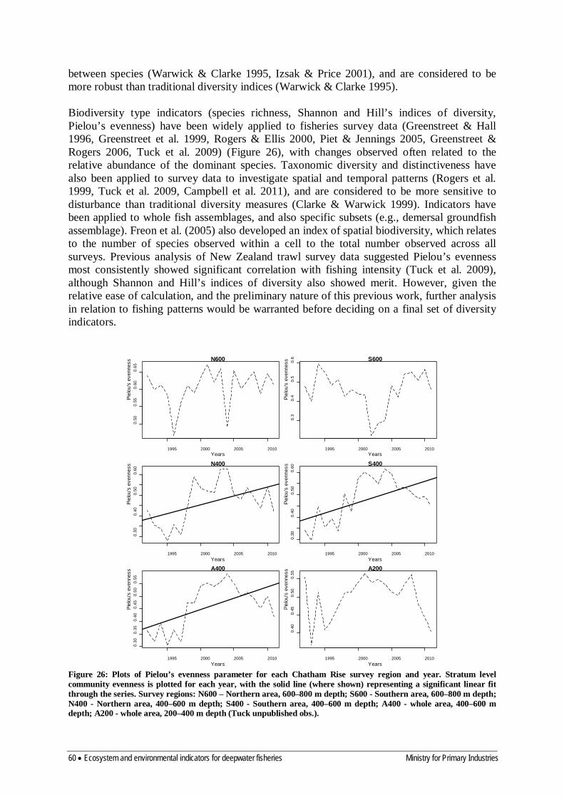
60 • Ecosystem and environmental indicators for deepwater fisheries Ministry for Primary Industries
between species (Warwick & Clarke 1995, Izsak & Price 2001), and are considered to be more robust than traditional diversity indices (Warwick & Clarke 1995). Biodiversity type indicators (species richness, Shannon and Hill’s indices of diversity, Pielou’s evenness) have been widely applied to fisheries survey data (Greenstreet & Hall 1996, Greenstreet et al. 1999, Rogers & Ellis 2000, Piet & Jennings 2005, Greenstreet & Rogers 2006, Tuck et al. 2009) (Figure 26), with changes observed often related to the relative abundance of the dominant species. Taxonomic diversity and distinctiveness have also been applied to survey data to investigate spatial and temporal patterns (Rogers et al. 1999, Tuck et al. 2009, Campbell et al. 2011), and are considered to be more sensitive to disturbance than traditional diversity measures (Clarke & Warwick 1999). Indicators have been applied to whole fish assemblages, and also specific subsets (e.g., demersal groundfish assemblage). Freon et al. (2005) also developed an index of spatial biodiversity, which relates to the number of species observed within a cell to the total number observed across all surveys. Previous analysis of New Zealand trawl survey data suggested Pielou’s evenness most consistently showed significant correlation with fishing intensity (Tuck et al. 2009), although Shannon and Hill’s indices of diversity also showed merit. However, given the relative ease of calculation, and the preliminary nature of this previous work, further analysis in relation to fishing patterns would be warranted before deciding on a final set of diversity indicators.
Figure 26: Plots of Pielou’s evenness parameter for each Chatham Rise survey region and year. Stratum level community evenness is plotted for each year, with the solid line (where shown) representing a significant linear fit through the series. Survey regions: N600 – Northern area, 600–800 m depth; S600 - Southern area, 600–800 m depth; N400 - Northern area, 400–600 m depth; S400 - Southern area, 400–600 m depth; A400 - whole area, 400–600 m depth; A200 - whole area, 200–400 m depth (Tuck unpublished obs.).
1995 2000 2005 2010
0.50
0.55
0.60
0.65
N600
Years
Piel
ou's
eve
nnes
s
1995 2000 2005 2010
0.3
0.4
0.5
0.6 S600
Years
Piel
ou's
eve
nnes
s
1995 2000 2005 2010
0.30
0.40
0.50
0.60
N400
Years
Piel
ou's
eve
nnes
s
1995 2000 2005 2010
0.30
0.40
0.50
0.60
S400
Years
Piel
ou's
eve
nnes
s
1995 2000 2005 2010
0.30
0.35
0.40
0.45
0.50
0.55
A400
Years
Piel
ou's
eve
nnes
s
1995 2000 2005 2010
0.40
0.45
0.50
0.55
A200
Years
Piel
ou's
eve
nnes
s

Ministry for Primary Industries Ecosystem and environmental indicators for deepwater fisheries • 61
8.3 Community composition While diversity measures provide one approach to describing community composition, a range of other indicators are also available, based on total, or proportional abundance or biomass of different habitat groups (e.g. demersal fish) (Cury et al. 2005). Changes in total biomass of fish have been interpreted in relation to levels of fishing pressure (Fogarty & Murawski 1998, Rochet & Trenkel 2003), although total fish biomass may depend on several factors such as food availability, water temperature or fishing (Piet 2001). Biomass, or proportions of species of interest (targeted, vulnerable, key prey), or ratios of trophic or habitat groups (piscavores, demersal fish), have been widely used as indicators, and can be easier to interpret than diversity indicators (Figure 27).
Figure 27: Plots of the Chatham Rise total survey (black dashed line) and target species (grey dashed line) biomass for each survey region, with the solid line (where shown) representing a significant linear fit through series. Survey regions: N600 – Northern area, 600–800 m depth; S600 - Southern area, 600–800 m depth; N400 - Northern area, 400–600 m depth; S400 - Southern area, 400–600 m depth; A400 - whole area, 400–600 m depth; A200 - whole area, 200–400 m depth (Tuck unpublished obs).
Total biomass variability is a measure for comparing the variability of total community biomass with individual species within that community (Duplisea et al. 1997, Blanchard & Boucher 2001). In “healthy” communities, individual species will compensate for each other, and total biomass is less variable than that of the individual species. In “stressed” communities, variation of individual species are more independent (species may no longer be energy limited, and inter-species interactions may have less influence), and variation in total
1995 2000 2005 2010
050
0015
000
2500
0 N600
Years
Tota
l bio
mas
s
1995 2000 2005 2010
020
000
4000
060
000 S600
Years
Tota
l bio
mas
s
1995 2000 2005 2010
010
000
3000
050
000
N400
Years
Tota
l bio
mas
s
1995 2000 2005 2010
020
000
4000
060
000
8000
0 S400
Years
Tota
l bio
mas
s
1995 2000 2005 2010
050
000
1000
0015
0000
A400
Years
Tota
l bio
mas
s
1995 2000 2005 2010
050
000
1000
0015
0000 A200
Years
Tota
l bio
mas
s

62 • Ecosystem and environmental indicators for deepwater fisheries Ministry for Primary Industries
biomass can increase. Interannual variability in the stock size of individual species has also been considered as an indicator of stock “health” (Hsieh et al. 2006, Anderson et al. 2008), as exploited species show greater temporal variability in abundance, with authors suggesting that this is related to fishery induced truncation of age structure, reducing the population’s capacity to buffer environmental events (Hutchings & Reynolds 2004). Some species (e.g., squid) show very high levels of natural variability, and may not be appropriate for inclusion in this sort of analysis. Some species are considered to be particularly sensitive to the effects of fishing or other disturbances (possibly due to a combination of life history characteristics: slow growth, large size and age at maturity, and low fecundity), and their abundance or size structure may provide an indicator of ecosystem health. Skates, rays, and other species considered at risk (e.g., IUCN Red list; DOC NZ Threat Classification System list) have been examined in this way in some areas (Walker & Hislop 1998, Rogers & Ellis 2000, Maxwell & Jennings 2005, Tuck et al. 2009). Other resilience or productivity (Musick 1999), or extinction vulnerability (Cheung et al. 2005) classification approaches in relation to fishing pressure based on species life history characteristics (including maximum length and age, age at maturity, fecundity, natural mortality and geographic range) are also readily available within the Fishbase system (www.fishbase.org). Indicators can be in terms of absolute abundance (or biomass), or expressed as a percentage of total survey biomass, and power to detect change is increased by developing composite indicators (e.g., combined biomass of threatened species, rather than individual species indices) (Maxwell & Jennings 2005). The New Zealand Threat Classification System (Townsend et al. 2008) has recently been applied to marine invertebrates (Freeman et al. 2010), identifying umbrella octopus and Giant squid as being in the “nationally critical” category. Applying the previous DOC classification to marine fish only identified White pointer shark (Great white) and Basking shark as “gradually declining” within the “chronically threatened” class (Hitchmough 2002) (these are covered in Section 10), although other species were also classified as “at risk”. The Giant grouper and Spotted black grouper are protected under the Wildlife Act 1953, although both these species are coastal, and would be unlikely to be caught in deepwater fisheries. Stock assessments tend to focus on the important commercial species, but surveys provide valuable information on numerous taxa. Mueter & Megrey (2005) examined linear trends in survey CPUE and frequency of occurrence over time series for individual species, but examined the distribution of slopes observed across all taxa in relation to simulated slopes under a null hypothesis (no overall trend) to evaluate whether the observed distributions had significantly more species than expected showing a decline. Differences (compared to expected distribution of change) were identified between commercial and non-commercial species, and also between areas with different fishing pressures. While not an indicator as such, community composition from trawl survey data has also been examined using multivariate statistical approaches to investigate spatial and temporal changes (Atkinson et al. 2011). Dominance patterns in fish communities have been examined through Abundance Biomass Comparison (ABC) curves and the W statistic (Jouffre & Inejih 2005, Yemane et al. 2005). In an examination of spatial patterns in trawl survey series, the W statistic was consistently found to be negatively correlated with fishing intensity (Tuck et al. 2009).

Ministry for Primary Industries Ecosystem and environmental indicators for deepwater fisheries • 63
8.4 Size composition Ecologically, the size composition of a community integrates a large quantity of information about the processes underlying community dynamics (productivity, mortality, and life history strategies)(Pope et al. 1987). In addition, fishing may lead to substantial modifications in the size structure of exploited populations because i) high-value, generally larger species are targeted by fisheries, (ii) fishing gears are size selective, often designed to catch larger fish and let smaller ones escape, (iii) the cumulative effects of fishing (over the life of a cohort) lead to fewer older (larger) fish, and (iv) large sized species tend to be more vulnerable as they have lower potential rates of increase. Size based indicators (SBIs) are therefore potentially a powerful approach to monitor the effects of fishing on populations and communities, and a wide range of size based indicators are available. Some, as described above, are applicable to single species, but most have been applied across whole fish communities (Shin et al. 2005). Indicators range from relatively simple indices such as mean or maximum size (or weight) in a population or community, mean length at age, and proportions of large individuals through to more complex indices such as the slope and intercept of size spectra (Shin et al. 2005). Mean length across a whole fish community is relatively insensitive to trends in recruitment (Ault et al. 2005), and has been used to detect differences between sustainable and non-sustainable rates of exploitation, although statistical power to detect trends in mean size from surveys is thought to be low (Nicholson & Jennings 2004). The proportion of fish over 30 cm in the community has been used in the North Sea to discriminate between high, medium and low levels of fishing effort (Greenstreet & Rogers 2006). Mean length at maturity has also been used at the community level within the North Sea to discriminate between levels of fishing effort (Greenstreet & Rogers 2006). Although species richness and relative abundance of species in a series of samples may be highly variable, the biomass and numbers of individuals (pooled across all species) decreases log-linearly with size. The slope and intercept of these size spectra are properties which can be compared between communities or over time, quantifying the relative abundances of small and large fish and the overall productivity of the system (Figure 28). In theory, differences in productivity appear as differences in intercepts, while differences in transfer efficiencies and mortality appear as differences in slope, although in reality, slopes and intercepts are often correlated, and cannot be interpreted independently. Theoretical simulations have shown that fishing might also destabilise biomass flow, amplifying temporal oscillations, and making the size spectra more “wavy” (Rochet & Benoît 2012). The slope of size spectra appears to respond in a consistent way to changes in exploitation levels, and a decreasing trend in the slope has been observed in most areas studied, reflecting changes in size composition towards a relative decline in larger fish (Rice & Gislason 1996). Biomass spectra (log biomass (g.haul-1) and log body weight distributions) provide an alternative set of indicators. The biomass spectra follow a parabolic curve, and the curvature of the parabola, and body size and biomass at the parabola vertex have been used as indicators (Duplisea & Castonguay 2006). While the curvature is considered to be related to predator–prey body size ratio and specific production, and relatively insensitive to fishing, both the body size and biomass at the vertex would be expected to ultimately decrease as exploitation increased, although biomass may initially increase in the early stages of exploitation, owing to competitive release from the largest fish removed by new fisheries. These indicators are considered to be less sensitive to changes in size range end point gear catchability than spectra slope (Duplisea & Castonguay 2006).
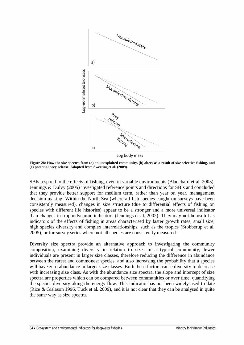
64 • Ecosystem and environmental indicators for deepwater fisheries Ministry for Primary Industries
Figure 28: How the size spectra from (a) an unexploited community, (b) alters as a result of size selective fishing, and (c) potential prey release. Adapted from Sweeting et al. (2009).
SBIs respond to the effects of fishing, even in variable environments (Blanchard et al. 2005). Jennings & Dulvy (2005) investigated reference points and directions for SBIs and concluded that they provide better support for medium term, rather than year on year, management decision making. Within the North Sea (where all fish species caught on surveys have been consistently measured), changes in size structure (due to differential effects of fishing on species with different life histories) appear to be a stronger and a more universal indicator than changes in trophodynamic indicators (Jennings et al. 2002). They may not be useful as indicators of the effects of fishing in areas characterised by faster growth rates, small size, high species diversity and complex interrelationships, such as the tropics (Stobberup et al. 2005), or for survey series where not all species are consistently measured. Diversity size spectra provide an alternative approach to investigating the community composition, examining diversity in relation to size. In a typical community, fewer individuals are present in larger size classes, therefore reducing the difference in abundance between the rarest and commonest species, and also increasing the probability that a species will have zero abundance in larger size classes. Both these factors cause diversity to decrease with increasing size class. As with the abundance size spectra, the slope and intercept of size spectra are properties which can be compared between communities or over time, quantifying the species diversity along the energy flow. This indicator has not been widely used to date (Rice & Gislason 1996, Tuck et al. 2009), and it is not clear that they can be analysed in quite the same way as size spectra.
Ministry for Primary Industries Ecosystem and environmental indicators for deepwater fisheries • 65
8.5 Trophodynamic (food-web) indicators Trophodynamic indicators measure the strength of interactions between different living components, and can be used to examine structural ecosystem changes (Cury et al. 2005). There are many data-intensive approaches to testing for change in emergent properties of marine ecosystems, including trophic spectrum (Gascuel et al. 2005), overhead, ascendency and capacity (Ulanowicz 1986, Ulanowicz & Norden 1990, Ulanowicz 2000), Finn’s cycling index (Fulton et al. 2005, Shannon et al. 2009) and thermodynamic indicators such as exergy and emergy (Jørgensen 2006). However, ecological indicators based on network analysis of food-webs tend to require more data, and be more sensitive to uncertainty in these data, than simpler indices based on biomasses of particular types of species present (Fulton et al. 2005). While some of this more basic information is available, most of the potential more complex trophodynamic indicators are beyond scope. On the basis of the data available, the application of trophodynamic indicators has generally focussed on the fish community alone, rather than other components of the ecosystem. From a review of 46 specifically trophodynamic indicators derived from models and emergent patterns (trophic cascades and regime shifts), Cury et al. (2005) proposed the following six trophodynamic indicators to reveal ecosystem-level patterns.
1. Catch or biomass ratios, the relative change in species (or functional group) composition within the catch can be quantified to characterise ecosystem changes. Such ratios are easily measurable and understood, and are often sensitive to fishing (Cury et al. 2005), and examples include the ratio of pisciverous to zooplanktiverous fish (Caddy & Garibaldi 2000) and the ratio of demersal catch to total catch (Cury et al. 2005).
2. The primary production required (PPR) to support catches in a system is expressed as
a percentage of total primary production available in the system, and can be used to compare the effects of fishing at different trophic levels, quantifying the ecological expense of fishing in an ecosystem (Pauly & Christensen 1995), but is dependent on realistic estimates of primary production.
3. Production or consumption ratios and predation mortality can be used to quantify the
relative importance of prey or predators, and the importance of predation or fishing mortality relative to total mortality in a particular group may be useful in tracking change in trophic structure (Cury et al. 2005). More recently, trophic interaction efficiency has been examined as an indicator addressing similar aspects of ecosystem dynamics (Daskalov et al. 2007).
4. Trophic level (TL) identifies the position of organism within a foodweb. TL tends to
increase with fish age (although lack of detailed information has meant that studies applying mean TL as an indicator have often only applied a single value for each species), and fisheries generally remove the older, larger predatory fish first, therefore reducing the mean TL of the remaining assemblage (Figure 29). A decline in TL may occur within and among species, leading to a decline in mean TL in catches, known as “fishing down marine foodwebs” (Pauly et al. 1998). Applying this indicator to commercial catches may be sensitive to changes associated with market forces (Branch et al. 2010), but applying the approach to survey data should provide a more

66 • Ecosystem and environmental indicators for deepwater fisheries Ministry for Primary Industries
robust measure of the trophic structure of the resident community, dependant on differences in catchability between species.
5. The Fishing-in-Balance (FiB) index examines whether the trend in catch over time is
consistent with the trophic level being fished, relative to a reference year (Pauly et al. 2000), and is thought to be a better indicator of ecosystem change than catch or catch composition, as it integrates across trophic levels (Garcia & Staples 2000), but requires knowledge of transfer efficiency between trophic levels.
6. Mixed trophic impact (at equilibrium) is a measure of the relative impact of a change
in the biomass of one component on the other components of the ecosystem (Ulanowicz & Puccia 1990), and can be used to identify groups that may have large trophic impacts on others, and so might be considered “ecologically important” species for use as indicators.
Figure 29: Plots of the Mean TL (assuming a single TL for each species, rather than any size effects) for each Chatham Rise survey region and year. Weighted stratum averages are plotted for each year, with the solid line (where shown) representing a significant linear fit through series. Survey regions: N600 – Northern area, 600–800 m depth; S600 - Southern area, 600–800 m depth; N400 - Northern area, 400–600 m depth; S400 - Southern area, 400–600 m depth; A400 - whole area, 400–600 m depth; A200 - whole area, 200–400 m depth (Tuck unpublished obs).
Other authors have applied alternative approaches. Using a methodology similar to size spectra, trophic spectra represent the distribution of abundance or biomass in a community by trophic level (Gascuel et al. 2005, Sosa-Lopez et al. 2005). These have been examined for
1995 2000 2005 2010
3.90
4.00
4.10
N600
Years
Mea
n TL
1995 2000 2005 2010
3.5
3.6
3.7
3.8
3.9
4.0 S600
Years
Mea
n TL
1995 2000 2005 2010
4.10
4.20
4.30
N400
Years
Mea
n TL
1995 2000 2005 2010
4.05
4.10
4.15
4.20
4.25
4.30
4.35 S400
Years
Mea
n TL
1995 2000 2005 2010
4.05
4.15
4.25
4.35 A400
Years
Mea
n TL
1995 2000 2005 2010
3.8
3.9
4.0
4.1
4.2
A200
Years
Mea
n TL

Ministry for Primary Industries Ecosystem and environmental indicators for deepwater fisheries • 67
New Zealand deepwater trawl surveys, with the data suggesting that there may have been some changes over the time series available (Tuck et al. 2009) (Figure 30).
Figure 30: MDS plot of pairwise P values (taken as measures of similarity) generated from KS tests of relative biomass trophic spectra over time for the combined southern 600–800 m depth strata on the Chatham Rise survey (Tuck et al. 2009). The plot indicates a gradual shift in the trophic spectra from the early 1990s (right side of plot) to the early 2000s (left side of plot), with the trophic spectra in more recent years similar to that in the late 1990s.
8.6 Recommended candidate indicators for Deepwater fish communities The fish communities are probably the most widely studied components of the deepwater marine ecosystem considered within this report, and trawl surveys are considered to provide the most useful data source for indicators, given that they are designed to provide standardised data on abundance and size composition over space and time. The indicators considered to be most useful in relation to deepwater fisheries, covering the aspects related to fish communities are: Target species – providing measures for that component of the community of most interest to the commercial fishing industry:
• Target species biomass • Species distribution.
Diversity and community composition – providing measures to examine spatial and temporal patterns in the species structure of the community:
• Total biomass
S600
199119921994
1995
1996 199719981999
2000
2001
2002
2003
2004
20052006
2007
2008
2009
2010
2011
2D Stress: 0.05

68 • Ecosystem and environmental indicators for deepwater fisheries Ministry for Primary Industries
• Community biomass ratios • Community diversity
Size composition – providing measures to examine spatial and temporal patterns in the size structure of the community:
• Proportion of large fish • Size (or biomass) spectra
Trophodynamics – providing measures to examine spatial and temporal patterns in the trophic web structure of the community:
• Mean trophic level • Trophic biomass ratios
9 BENTHIC COMMUNITIES AND HABITATS (SEA-FLOOR INTEGRITY) Benthic communities and habitats provide valuable ecosystem functions, through linking benthic and pelagic systems, and also providing habitat structure, but can be vulnerable to disturbance from mobile fishing gear. A number of habitat related indicators have been developed, considering individual species, community composition and the physical seafloor habitat (Fulton et al. 2004). The European Marine Strategy Framework Directive (MSFD) considers these within the “Sea-floor integrity” descriptor, and identifies two components; physical damage to substrate characteristics (particularly biogenic habitats), and the condition of the benthic community (Rice et al. 2012).
9.1 Substrate characteristics Seafloor substrates provide habitat for benthic communities, and to some extent, define habitat distributions. Biogenic substrates (e.g., mussel beds, sponge beds, corals) often have complex physical structure, providing three-dimensional habitats for a large variety of species, and can thus influence the structure and diversity of associated fauna, but are considered to be the most sensitive to physical disturbance. Bioengineers modify the seafloor environment by bioturbation (sediment reworking/burrowing) or by providing structure themselves. They can affect ecosystem functions by creating (through their own structure) or providing shelter from predation or erosion, habitats, displacement and mixing of sediments, transport of interstitial pore water, remineralisation of organic matter, and increased oxidation-reduction reactions in sediments (Meysman et al. 2006). Indicators include the spatial overlap of habitats with fishing activities (as described in Section 7), and also the physical changes to the seabed associated with fishing disturbance (e.g., acoustic roughness) (Tuck et al. 1998, Puig et al. 2012). The spatial overlap type indicators, particularly where fishing intensity data are available, can be combined with simple benthic production models, to then develop indicators relating estimated benthic biomass or production to the undisturbed level (Hiddink et al. 2006, Mormede & Dunn in press). Fishing intensity measures have also been combined with models of natural

Ministry for Primary Industries Ecosystem and environmental indicators for deepwater fisheries • 69
disturbance to estimate the probability that fishing disturbance exceeds natural disturbance, as an indicator of overall sea-floor integrity (Diesing et al. 2013). This specific indicator has been developed for a relatively shallow environment, and other measures may be more useful for deepwater environments (e.g., level of physical disturbance relative to natural disturbance), where natural disturbance would be expected to be lower. Indicators of bioengineers could be measures of abundance or distribution of the relevant key species, or extent of habitats.
9.2 Benthic communities The types of indicators relevant to address changes in benthic communities are generally similar to those described in the relevant sections on fish community indicators (particularly size and diversity based indicators, Section 8), although there are likely to be far less data available for benthic communities, particularly in deepwater, which may limit application of some indicators. Only additional indicators are discussed in detail here. As with fish communities, some benthic community species are more susceptible to damage from mobile fishing gear than others, due to factors such as life history traits, habitat or mobility (Jennings & Kaiser 1998, Eleftheriou 2000, Tuck & Hewitt 2013). This can lead to changes in community composition in disturbed communities, which can be examined using the same types of diversity and other community composition indicators as described for fish community data. Specific benthic community sensitivity indices have been developed in relation to biological traits (de Juan et al. 2009), and these can be used to categorise species or habitats (Hewitt et al. 2010) by vulnerability. The approach uses multivariate methods to combine biological traits that relate to size, age, rarity and vulnerability to disturbance, based on the abundance of the organisms. In addition, some benthic community groups are subject to measurable non-fatal anatomical damage (e.g. shell scars or damage in bivalves, loss of limbs in starfish) which may be useful surrogates for the impact of fishing on benthic communities (Witbaard & Klein 1994, Kaiser 1996, Ramsay et al. 2001), assuming that these species are selected by the sampling gears available. While trawl surveys and observer sampling on commercial fishing vessels provide a good opportunity to collect data on benthic communities, the selectivity of the trawl gear for these species is generally low, and samples collected in this way may not be particularly good representations of actual benthic communities. As with the fish indicators described above, pressures that decrease productivity or increase mortality will lead to communities with fewer individuals surviving to larger sizes. Size based indicators relating to benthic communities are likely to be limited to the proportion greater than some specified size, and even for these, specific benthic community orientated sampling activities may be required. Indicators related to fishing pressure, removals from, or protection of specific habitats, and the identification of those habitats (e.g., using BOMEC) are discussed in Section 7.
9.2.1 Deepwater hard corals The EU project Coralfish http://eu-fp7-coralfish.net/ has recently coordinated a number of studies on deepwater corals, and in particular the interactions between corals, fish and fisheries. Deepwater corals are considered as a special category of deepwater communities.

70 • Ecosystem and environmental indicators for deepwater fisheries Ministry for Primary Industries
Deepwater corals provide physical structure where they occur, and are very sensitive to physical impact from mobile fishing gear (Clark & Rowden 2009, Williams et al. 2010), and in some regions appear to support higher abundances of fish than areas without corals (Miller et al. 2012, Tracey et al. 2012), although direct linkages between the fish and corals are often uncertain. Deepwater corals are also considered to be particularly sensitive to ocean acidification (Turley et al. 2007, Guinotte & Fabry 2008, Tracey et al. in press). D’Onghia et al. (2010) found no significant differences in fish abundance between coral and non-coral habitats when long lining, but identified refuge effects in coral areas, and also suggested that the coral habitat acts as a spawning and nursery area for some species. A later study in the same region also identified fish community differences between coral and non-coral habitats in the absence of fishing (D'Onghia et al. 2012). Ballion et al. (2012) also suggested that deepwater corals provide fish nursery habitat. Deepwater corals are also likely to be some of the first groups to be affected by predicted shallowing of saturation horizons related to ocean acidification. All deepwater hard corals in the orders Antipatharia (black corals), Gorgonacea (octocorals), Scleractinia (stony corals), and Family Stylasteridae in Order Anthoathecata (hydrocorals) are protected in New Zealand. The Order Gorgonacea has recently been revised and all gorgonians are now in Order Alcyonacea (2010 amendment of Schedule 7A of the Wildlife Act 1953). Due to their protected status, deepwater corals have been the focus of a number of effects of fishing related studies. The distribution of the protected corals in relation to fishing effort, and the identification of areas where deep sea corals are at highest risk of interactions with commercial fishing gear are described in Tracey et al. (2011a). Baird et al. (2013) expands on the work by using additional sources of information relevant to the distribution of corals, including mapping of likely coral distributions using predictive models, and provides recommendations on any future research required to further improve the estimation of risk to protected corals from commercial fishing. Indicators could include quantities of coral caught, or spatial overlap of fishing with known areas of coral distribution (e.g. Clark & Tittensor 2010).
9.3 Recommended candidate indicators for Benthic communities and habitats Benthic communities and habitats provide a valuable link between the seabed and pelagic systems, and also provide habitat structure, thought to be important to some fish species. Benthic communities are generally poorly known in deepwater habitats, with research often focussed on specific groups (e.g., deepwater corals). Indicators measuring fishing disturbance in relation to benthic habitats are considered in Section 7.1.2. The indicators considered to be most useful in relation to deepwater fisheries, covering the aspects related to benthic communities are: Community or Seafloor integrity – providing an overall measure of benthic environment or community relative to “natural” conditions:
• Estimated benthic biomass or production relative to unfished levels • Fishing disturbance relative to natural disturbance
Community diversity and structure – providing measures to examine spatial and temporal patterns in the species structure of the community, and its vulnerability to fishing disturbance on the basis of life history traits:

Ministry for Primary Industries Ecosystem and environmental indicators for deepwater fisheries • 71
• Community diversity • Community and habitat vulnerability
Deepwater corals – providing measures of the risk of disturbance and level of fishery interaction for this group of New Zealand protected species:
• Coral distribution in relation to fishing pressure • Coral bycatch
10 TOP PREDATORS & THREATENED/PROTECTED SPECIES Indicators discussed here specifically address top predators and species legally protected in New Zealand waters (excluding deepwater corals, covered in Section 9.2). Other approaches to identifying ecologically vulnerable or threatened species are available (e.g., IUCN Red list, resilience to fishing pressure, extinction vulnerability to fishing), and these are considered within Section 8.3 (i.e., proportion of community biomass considered threatened).
10.1 Top predators The ecological viability of top predator populations (seabirds, marine mammals, and large sharks and rays sharks) is often taken as an indicator of ecosystem condition, as top predators are considered to integrate across variability at other levels in the ecosystem (Reid et al. 2005), and they may also have life history traits making them vulnerable to fishing (slow growth, low fecundity, large size). Top predators are widely used in monitoring the ecosystem effects of fishing krill in the Southern Ocean (Reid et al. 2005, Constable 2006), with information on the breeding of penguins, albatross, petrels, and seals collected, summarised and considered in management annually (Agnew 1997, CCAMLR 2004). Monitoring population size and breeding success of top predators as “bellweathers” of ecosystem health is also increasingly used elsewhere (Ainley 2002, Boyd et al. 2006) as they are recognised as potentially useful downstream integrators of change in the marine ecosystem, exploit marine resources at similar spatial and temporal scales to humans, and receive high public interest. However, given that predators respond in complex ways to many factors simultaneously, ascertaining the appropriate management response to change of a predator-based indicator is difficult (Boyd et al. 2006). In New Zealand, some key populations known to have interactions with fisheries are surveyed on a regular basis (e.g., Baker et al. 2012, Baker et al. 2013). Multispecies indicators, and/or indicators based on multiple metapopulations can be used to create a composite predator index that can improve generality, but research cost is often prohibitive (Boyd et al. 2006), and if individual populations are affected by different drivers, important signals may be lost by composite indices.
10.2 Threatened/protected species A number of top marine predators in New Zealand waters have been classed as threatened (Hitchmough 2002, Miskelly et al. 2008, Baker et al. 2010), and all marine mammals, almost all New Zealand seabirds, and a number of sharks and rays are protected under the Wildlife Act 1953. Other than the cephalopoda discussed in the fish community composition section, the New Zealand invertebrates classified as “nationally critical” by Freeman et al. (2010) are

72 • Ecosystem and environmental indicators for deepwater fisheries Ministry for Primary Industries
not relevant here, in relation to deepwater fisheries. However, a number of other taxa were identified as endangered or vulnerable (including protected deepwater corals) (Freeman et al. 2010), and distribution or incidence in bycatch of these species could be used as a pressure indicator, while abundance of these species could be used as a state indicator. Protected species known to interact with commercial fishing operations are:
• All marine mammals • All seabirds (except the black-backed gull) • All marine reptiles • Spotted Black Grouper (SBG) • Giant or Queensland Grouper (GGP) • White pointer shark (WPS) • Basking Shark (BSK) • Whale Shark (WSH) • Deepwater Nurse Shark (ODO) • Manta Ray (RMB) • Spinetail Devil Ray (MJA) • Deepwater hard corals
10.3 Candidate indicators The main aspects of these populations generally considered as indicators are population size and distribution, diet, and reproductive success (particularly for seabirds and pinnipeds, where juveniles can be surveyed at nesting sites and rookeries), although other indicators have also been developed related to interactions with fishing activities. Population surveys are routinely conducted for some key marine mammal and seabird populations with fishery interaction concerns, but far less data are available for protected fish, particularly the sharks and rays. Recognising the data-poor nature of many shark fisheries, specific indicator approaches have been developed to assess the response of the populations to fishing pressure (Clarke et al. 2011), and are under development for New Zealand populations (Clarke et al. 2013). Indices of population size and distribution provide an indication of the “health” of the population, although these may be difficult to interpret for migrant species which only spend a small portion of their life within New Zealand waters. Indicators could relate to the number of species listed as threatened, individual species abundance indices or population distributions, or an aggregate index combining a number of species. In the same way that composite indices of vulnerable species have greater power to detect changes than individual species trends (Maxwell & Jennings 2005), combined predator indicators appear to be more useful than individual ones, when associated with the same prey. A wide range of indices of predator performance for four Antarctic predator species (Antarctic fur seal, Gentoo penguin, Macaroni penguin and Black-browed albatross) were examined in relation to the abundance of their main prey (Reid et al. 2005), with multivariate indices, combining variables (including population size, breeding success, offspring condition, meal mass and foraging trip duration) from all four species into a single index, providing a better fit to prey abundance than any of the individual indices. Underhill & Crawford (2005) developed individual seabird population indices for a region, and integrated them into single total community index. The appropriateness of regional or species type

Ministry for Primary Industries Ecosystem and environmental indicators for deepwater fisheries • 73
composite indicators in the New Zealand context needs to consider whether the individual species are being affected by the same drivers, as otherwise individual population signals may be lost. In addition to population and distribution trends which would be relevant to all species, trends in median size (relative to maturity), sex ratio, and percentage catch composition are considered to be useful indicators for shark species (Clarke et al. 2011), and are being used to monitor populations elsewhere in the Pacific. Reproductive success as an indicator of the impacts of fishing has probably been best studied for seabirds (Goni 1998), with evidence of effects related to overfishing of prey species, availability of discards for scavenging, and the removal of larger predatory fish which chase prey fish into seabird foraging zones (Flint 1999). Data are also available for New Zealand sea lions (e.g., Baker et al. 2012, Chilvers 2012), with annual surveys providing an index of pup production for some key populations. Richard et al. (2011) examined annual potential fatalities (APF) (from all New Zealand fishing) in relation to potential biological removals (PBR; the amount of human-induced mortality a species can sustain without compromising its persistence), and identified eight species of seabird at risk (annual potential fatalities exceeding potential biological removals), although some of these are only likely to be at risk from inshore fisheries, rather than the deepwater activities considered here. The ratio of annual potential fatalities to potential biological removals (for individual species, aggregated across groups, or the numbers of species where the ratio exceeds 1) could provide an indicator of relative fishing impact on populations. Other indicators have also been developed using a spatially explicit Productivity – Susceptibility analysis, to determine the probability of seabird – fisheries interactions, and the risk of these interactions having adverse effects (Fillipi et al. 2010).
10.4 Recommended candidate indicators for Top predators and Threatened/Protected species
The top predators and protected species encompass a wide range of “high profile” species, with different types of data, and hence indicators available. In the New Zealand context, indicators are likely to be calculated at the individual species level, but where populations are affected by the same drivers in the same region (e.g., bycatch by the same fleet), composite indicators may be appropriate. The indicators considered to be most useful in relation to deepwater fisheries, covering the aspects related to top predators and threatened/protected species are: Population trends:
• Abundance estimates from direct surveys (seabirds, marine mammals) or CPUE indices (sharks, rays, other fish) for individual species
• Distribution • Breeding success (seabirds and pinnipeds) • Population structure (median size and sex ratio) in bycatch (sharks)
Fishery interactions:
• Estimated fishery interactions and mortalities (seabirds and marine mammals)

74 • Ecosystem and environmental indicators for deepwater fisheries Ministry for Primary Industries
• Percentage catch composition (for shark bycatch species) • Risk ratio (e.g. APF/PBR or similar)
11 ROLE OF OBSERVERS This section provides a review of the New Zealand Government Fisheries Observer Programme at-sea data collection on commercial vessels in relation to deepwater stocks within the New Zealand region. A summary is provided of existing data collection procedures for the Observer Programme, Observer vessel placement, at-sea data recording required for various fishing methods, and the data forms used in all fisheries. We describe the identification tools available, recent refinements of at-sea sample collection, confidence in data for fish as well as benthic fauna, including VME taxa and protected corals. The MPI databases relevant to observer programme deepwater fisheries data collection are listed in Section 16.6.
11.1 Overview The use of fishery observers is becoming routine in fisheries worldwide. Fishery observers carry out a wide variety of duties, including collection of information on catch composition and discards, bycatch of endangered or protected species, environmental variables, and monitoring of adherence to regulations. The data they collect offers an additional source of ecosystem and environmental information for use with ecosystem indicators. This review summarises the role of the observer programme at-sea data collection in relation to deepwater stocks and species within the New Zealand regions and Ross Sea. The data collection is described and evaluated in relation to its use to formulate and monitor ecosystem and environmental indicators. Onboard observations can provide a wealth of information both on fishing practices and the state and dynamics of the ecosystem, although it must be remembered that as fishers follow their target species, rather than covering the whole ecosystem in a random manner, the “statistical sampling design” of these observations can be somewhat problematic. The types of indicators that could be produced from data collected currently include, for example, those that are derived from sized-based data, from the taxonomic diversity and distinctiveness of bycatch species, from the bycatch rates of indicator species or species groups, and from environmental measurements. However, the “preferential” nature of observer sampling (denser sampling in areas of high fishing intensity) means that careful analysis is required for deriving indicators for the ecosystem, as classical spatial statistical analysis methods are biased under such designs (Diggle et al. 2010, Gelfand et al. 2012). Given the history of observer coverage and the planned increase in deepwater fishery observer coverage, the Observer Programme may provide a substantial source of data for the calculation of indicators.
11.2 The New Zealand Government Fisheries Observer Programme The New Zealand Exclusive Economic Zone (EEZ) was declared on 1 April 1978. Since then

Ministry for Primary Industries Ecosystem and environmental indicators for deepwater fisheries • 75
The Ministry for Primary Industries (MPI) (previously the Ministry of Fisheries, MFish and the Ministry of Agriculture and Fisheries, MAF), has collected catch and fishing effort information from all fishing vessels operating within the EEZ and New Zealand vessels operating outside the EEZ. In June 1985 the intention to establish an Observer programme to monitor the activities of large trawlers operating in the New Zealand EEZ was announced, and the first observed fishing event took place in April 1986. The Territorial Sea and Exclusive Economic Zone Act empowers the Primary Industries Minister to place Observers on foreign fishing vessels. The Fisheries Act 1996 contains empowering legislation for the placement of Observers on New Zealand registered vessels. This includes both foreign-owned vessels chartered by New Zealand fishing companies and New Zealand-owned and operated vessels. The Observer Programme is managed by the MPI Observer Services Group, and is funded from levies on the fishing industry. In addition to the catch and fishing effort information MPI is required to collect, the Department of Conservation (DOC) through the Marine Species and Threats Programme (previously Conservation Services Programme (CSP)), have a statutory role to monitor and collect data on the interactions between commercial fisheries and protected species within the New Zealand’s Exclusive Economic Zone (EEZ). As such DOC also funds, through industry levies, a number of government observer sea days each year. MPI Observers have a wide range of existing tasks, and it is unlikely additional duties could be considered, other than for perhaps short term specific projects. This review focusses more on making best use of the data collected.
11.3 Review of existing data and procedures
11.3.1 Observer key roles The key roles of the New Zealand government observer programme (of relevance to indicators) and as described in the MPI Observer Manual are to:
• Determine and record all catch effort information for each fishing event (e.g., trawl, longline set).
• Approve and record quota species discards according to regulations. • Obtain biological data and samples on target and other species as required. • Observe the vessel's compliance or lack of compliance with fishing regulations, and
document infringements of regulations when observed. • Record details of incidentally caught marine mammals/birds and the behaviour and
occurrence of marine mammals/birds in the fishing areas. • Collect specimens for DOC, NIWA and other recipients.
In addition, observers are also required to record interactions between protected coral species and commercial fishing operations, and a portion of the overall observer coverage is targeted at protected species bycatch in selected fisheries. This role requires observers to:
• Monitor and record the nature and extent of interactions of protected species with fishing operations.

76 • Ecosystem and environmental indicators for deepwater fisheries Ministry for Primary Industries
• Report on the efforts made to mitigate the adverse effects of commercial fishing on protected species, including both use of specific devices and operational practices such as offal management.
• Report on live captures of protected species, noting whether or not they are treated humanely and released promptly.
• Recover specimens of dead protected species for identification and /or autopsy. • Record on a daily basis the numbers and behaviour of marine mammal and
seabird species seen around the fishing vessel. • Carry out other tasks (e.g., noting the types of fish discard species and offal produced,
and warp-strike observations) as required.
The protected species information can be used to identify where the most significant interactions are occurring and can inform development and application of strategies to minimise adverse impacts. The observed interactions (mortalities and specimens released alive) between protected species (including corals) and commercial fishing vessels have been summarised at a coarse level to inform where fishing effort, observer coverage, and captures occur, so that potential gaps in monitoring can be identified along with high risk areas and time periods in various fisheries (Ramm 2011).
11.3.2 Observer vessel placement and coverage Observers are placed on vessels in the deepwater fleet targeting the fish stocks and species listed in the Appendix (Section 16.1). Specific projects requiring observer services are prioritised, and where appropriate, costs divided between MPI and DOC. The coverage that can be achieved is sometimes limited by logistical constraints such as the availability of trained observers and vessel availability. The Observer Optimisation Programme, led by MPI Science Group, regularly meets to discuss the allocation of observers, rates of coverage in the fleet and statistical sampling requirements per trip. The allocation of observer days per fishery is determined by the MPI science group, and is passed to MPI Observer Services to implement. For the 2011–12 fishing year there were over 5500 observer days allocated to deepwater fisheries within the New Zealand EEZ, and about 800 of these were funded by DOC (see http://www.fish.govt.nz/). In addition to these, almost 1500 observer days (managed by Observer Services) were funded directly by the fishing industry, as required for Vessel Specific Conversion Factor testing, fishing operations outside of the EEZ (including the Antarctic), and monitoring of high-risk Foreign Charter vessels (FCVs). In addition to the usual coverage of the domestic deepwater fleet, as of 1 October, 2012, MPI have been required to place observers on all FCVs. One of the recommendations made by the FCV Review held in 2012 was that 100% observer coverage should occur on FCVs. It is highly likely that an increase in the number of trained observers will be required to meet this recent development. Details of observer coverage (total observed fishing events by target fishery, and recent annual mean) are provided in the Appendix (Section 16.2), with spatial distribution of coverage presented in 16.3. Most observer activity has focussed on the hoki, squid and orange roughy fisheries (average of over 1000 observed events annually since 2006),

Ministry for Primary Industries Ecosystem and environmental indicators for deepwater fisheries • 77
although fisheries for oreos, jack mackerel, ling, scampi, southern blue whiting and hake have each had an annual average of over 300 observed events since 2006. Numbers of events by fishing method and year are presented in Section 16.4. After 1986–87 the level of coverage of deepwater fish species trawling was generally between 5000 and 9000 trawls per year. Coverage of deepwater bottom longline fishing (almost exclusively targeting ling) began in 1992–93 and in most years has been at a level of 200–500 sets per year, but was much higher in 2001–02 and 2002–03. Observer Programme protocols are that, on a solo trip, the observer must observe a minimum of two-thirds (66.66%) of all tows, and depending on the number of tows each day, solo observers normally see 70 to 100% of hauls. If two observers are on board, the protocol states they must observe 100% of the hauls between them (Martin Cryer, MPI, pers. comm.).
11.3.3 At-sea data recording Instructions and data collected at sea by observers are summarised below for each fishing method, not comprehensively, but with regard to information which is potentially useful as sources of deep-sea ecosystem and environmental information. Bottom and mid-water trawling, targeting commercial fish species such as black and smooth oreos, orange roughy, alfonsino, black cardinalfish, and southern blue whiting, occurs throughout the NZ EEZ in depths ranging primarily from 200 m to 1500 m. Bottom long-lining is also a key deep-sea fishing method, especially for ling. Although purse seining, set-netting, surface longlining, and trolling fishing methods target fish in surface waters, they are included here because other biological and environmental data may be collected during these fishing activities which could be used to construct useful ecosystem indicators. Trawling is the main fishing method covered by observers, and a considerable amount of information is collected, using a range of forms, as prescribed in the Observer Work Schedules and Practices in the Observer Manual. Instructions are given to observers on how to fill out the various relevant forms, which include:
• Catch Effort Log Book (CELB) • Tori Line Details Form • Observer SLED Details Form • Trawl Gear Details Form • Benthic Materials Form • Protected Species Abundance Form • Length Frequency Forms (LF and MDBD (Middle Depth Biological Data)) • Non-Fish By-Catch Reporting
The standard catch effort form was used to record details of all catch species from trawl fishing until a benthic bycatch form, the Benthic Materials Form, was introduced in October 2007 to separately record by-catch of invertebrate species and inorganic material. Some forms, such as the trip log, protected species abundance, and length frequency forms, are common to all observed fishing methods, and other forms are specific to one method or a subset of fishing methods. A summary of all forms used by observers to collect data across each of these fishing methods is provided in Table 2, and further details are briefly described
78 • Ecosystem and environmental indicators for deepwater fisheries Ministry for Primary Industries
in Section 16.5. The MPI databases relevant to observer programme deepwater fishery data collection are described in Section 16.6. Photographs and videos are required to be taken in some instances, e.g., for the identification of live released protected species, for recording the nature of protected species interaction, and for documenting mitigation devices and their function. Observers have also collected other data in specific studies. Observers examined fish stomachs from highly migratory species on surface longline trips to provide diet information (97 101 stomachs between 1994 and 2012), although most prey items were identified only into broad categories, and comprehensive descriptions of diet could only be produced for the 12 most frequently sampled species (Horn et al. 2013c).

Ministry for Primary Industries Ecosystem and environmental indicators for deepwater fisheries • 79
Table 2: MPI observer forms completed by fishery.
Form type Traw
ling
Bot
tom
long
linin
g
Purs
e Se
inin
g
Set N
ettin
g
Surf
ace
long
linin
g
Trol
ling
Trip log X X X X X X Deck log X X
Catch Effort Log Book X Tori Line Details X
Warp Strike X SLED Details X
Trawl Gear Details X Skiff, spotter gear details X
Benthic Materials X X Protected Species Abundance X X X X X X
Length Frequency X X X X X X Non-Fish By-Catch Reporting X X X X X X
Bottom Longline Catch Effort Data X Setting Observations X X X Hauling Observation X X
Trolling Hourly Observation X Trolling configuration X
Trolling fishing gear X Vessel activity X
Net Gear Details X X Setnet Catch/Effort X
Stomach sampling/samples form1 X X Pacific (Northern) Bluefin stomach sampling1 X X
Meal plant usage X Snood log X
Bait log X Temperature calibration2 X
1. These forms may contain information pertaining to the migration of juveniles of deepwater species to the surface waters (e.g., data on juvenile smooth oreo, which have been and may continue to be found in the stomach contents of pelagic species). 2. Typically no temperature recording equipment is provided to observers (Kerry Huston, Fisheries Observer Officer, MPI, pers. comm.) and so these forms are rarely used.
11.3.4 Use of observer data Observer data from New Zealand fisheries are regularly used to support a range of research projects, including: estimating bycatch and discards in deepwater fisheries (e.g., Anderson 2012, and the current MPI project DAE201002B); examining the distribution of protected corals in New Zealand waters (Tracey et al. 2011a, Baird et al. 2013); summarising the capture of seabirds, marine mammals, and turtles in New Zealand commercial fisheries (Abraham & Thompson 2011, Ramm 2011); carrying out risk assessments for, and managing impacts of, incidental seabird mortality associated with New Zealand fisheries in the NZ EEZ (Rowe 2010); examination of the age, growth, and size structure of commercial fish species (Anderson & Doonan 2010); examination of the diet of commercial fish species (e.g., Dunn et al. 2010a); and investigating biological questions such as establishing the timing and location of spawning activity (Anderson 2006).

80 • Ecosystem and environmental indicators for deepwater fisheries Ministry for Primary Industries
Some of the information available in these publications, several of which report on regularly updated analyses, may be useful as indicator statistics with little or any modification. For example, in Anderson (2012), bycatch rates in the scampi trawl fishery are provided for main species and species groups by area and year since the 1990–91 fishing year. The scope of these bycatch investigations has subsequently been expanded so that, in the MPI project DAE201002, annual bycatch rates for a large number of species in a range of deepwater fisheries are being produced. Similarly, Abraham & Thompson (2011) provide estimates of the number of captures of a range of seabirds, marine mammals, and turtles in commercial fisheries for the years 1998–99 to 2008–09.
11.4 Identification tools and data accuracy Consistent with the requirements of the NZ Fisheries Act and the NZ Biodiversity Strategy, there has been increased research into examining trends in the abundance of “associated or dependent species”, i.e. non-target fish and invertebrate species associated with, or impacted by commercial fishing. High quality field identification is the foundation of good research, and improved identification guides have been developed to facilitate analyses and help with the development of accurate risk assessments of fisheries’ impacts on benthic habitats. The recording of certain bycatch from observed fishing has been shown to be robust and has vastly improved in recent years with concerted efforts to collect and ground-truth these data (returning samples for laboratory identification) and with the production of identification guides to aid at-sea identification. Commercial fish species identification has been very good, but there have always been difficulties in identifying certain species (e.g., mackerels, arrow squids). Some of the common bycatch groups have also proved difficult or time consuming to identify properly (e.g., rattails, deepwater dogfishes and other sharks) with generic codes such as RAT, DWD, and SHA in frequent use. The quality of the fish identification is likely to have improved since the recent publication of a set of fish identification guides (McMillan et al. 2011a, McMillan et al. 2011b, McMillan et al. 2011c), especially the identification of the less common species. Prior to the production of these guides, “New Zealand fish, a complete guide” (Paulin et al. 1989) and an observer programme in-house guide “Bony fish & crustacean catch sampling” (covering mainly commercial species) were the main resources for observers.
Two main field guides are supplied to observers for identification of seabirds, “The Hand Guide to the Birds of New Zealand” (Robertson & Barrie 2001) and “Albatrosses, Petrels and Shearwaters of the World” (Onley & Scofield 2007). Where taxonomy is in a state of flux, inserts to these books are supplied to ensure standardised reporting. Seabirds killed during observed fishing operations are retained for autopsy where possible, with experts typically confirming 70–80% of observer identifications (e.g., Bell 2013). Two main field guides are supplied to observers for identification of marine mammals, “Whales and Dolphins of New Zealand and Australia” (Baker 1983) and “Marine Mammals of Australia and New Zealand” (IFAW). Accuracy of observer identification of the species most frequency associated with deepwater fishery interactions is considered to be good (L. Torres, pers comm.). Deepsea invertebrate (Tracey et al. 2011b) and coral (Tracey et al. 2008) identification guides are provided to observers, and through use of these and their predecessors since 2005, the

Ministry for Primary Industries Ecosystem and environmental indicators for deepwater fisheries • 81
taxonomic level to which samples are successfully identified at sea has improved considerably. Prior to the publication of these guides observer identification of invertebrates relied on publications such as ‘A guide to some common offshore shrimp and prawn species of New Zealand’ (Webber et al. 1990) and various FAO Guides. Levels of the identification accuracy have been examined for some observer collected benthic fauna. Examination of data from the Ross Sea and New Zealand EEZ showed that for most groups, the observer classifications were reasonably accurate (88% accuracy) (Parker et al. 2009, Tracey et al. 2010), although in particular, problems in distinguishing some sponges and corals remain, particularly for identification to the species level. Accuracy was much improved at grouped taxonomic levels (Tracey et al. 2011b). This finding highlights the caution required when interpreting observer data. A higher grouping of codes provides an understanding of the key groups taken as by-catch but the value of identifying the corals to the lowest taxonomic level is considered paramount to understanding impacts on the region’s biodiversity. Benthic invertebrates and fish samples taken during research trawls and by observers on fishing vessels have regularly been returned for identification by experts. Revised identification data are loaded by the Data Manager (NIWA) into cod and trawl databases.
82 • Ecosystem and environmental indicators for deepwater fisheries Ministry for Primary Industries
12 CONCLUSIONS
12.1 General conclusions There are a number of different purposes of developing ecosystem indicators related to fisheries management. These include:
• Relating trends/information in climate, environmental or oceanic conditions to productivity of a species or stock (e.g. year class strength) for use in single-species management.
• Early-warning systems for regime shift (especially climate, oceanographic and primary-production indicators).
• Headline indicators for monitoring, communicating and comparing overall change in ecosystems.
• Indicators to monitor for long-term ecosystem erosion or reduced resilience. • Adding climate/oceanographic context to observed fisheries variability and change.
There is general consensus that monitoring a suite of indicators measuring a range of ecosystem aspects is more appropriate than focussing on a single indicator or ecosystem component. However, the best suite of indicators will be different for different purposes. Clarity of purpose for the use of indicators within MPI is hence likely to lead to better outcomes.
12.2 Climate, oceanographic, environmental indicators Environmental indicators (i.e., abiotic rather than biological measures) are desirable as context for ecosystem indicators, and to assist in identifying possible causes for patterns in ecosystem indicators. Studies investigating regime shifts in marine ecosystems are likely to be particularly useful in identifying potential environmental indicators. Long term trends, overlaid by decadal and interannual fluctuations, in phytoplankton abundance have been identified worldwide, and such indicators are likely to be very valuable in explaining some of the patterns observed in biological and fisheries indicators. A suite of climate indicators are available for the New Zealand region, including Interdecadal Pacific Oscillation (IPO), Southern Oscillation Index (SOI) and Antarctic Oscillation/ Southern Annular Mode. These describe changes to the principal spatio-temporal modes of variability in the regional climate system and are likely to have effects on New Zealand marine ecosystems. However, how variation in these modes affects marine organisms and communities is not well known. New Zealand oceanography is observed by satellite data: sea surface height/satellite altimetry (SSH), sea surface temperature (SST), incident light (Photosynthetically Active Radiation, PAR), surface chlorophyll-a concentration (as a proxy for phytoplankton biomass) and net primary productivity (NPP). These satellite measurements cover the whole New Zealand region at spatial scales of typically 1 km, repeat cycles of 1–16 days, and for durations in excess of 12 years. While considerable satellite remote sensing data are available, further analysis of them are required to determine the trends and variability of most relevance to fisheries.

Ministry for Primary Industries Ecosystem and environmental indicators for deepwater fisheries • 83
In comparison, long-term in situ measurements of oceanography and plankton are sparse. Currently scientific oceanographic data are collected to add to our understanding of processes relevant to regional oceanography and water chemistry rather than for monitoring purposes. In situ datasets that may be relevant to fisheries indicators are:
• Ocean SITES – stations in subtropical/sub-Antarctic waters (12 year time series – T, S, fluorescence, currents, POC flux).
• Coastal time series (14 yrs - T, S, fluorescence, currents, nitrate). • Otago transects (pCO2, pH, nutrients, Chl-a). • Argo (partnership with Scripps, UoW, CSIRO). • Deploying floats for Deep Argo. • XBT lines in NW Pacific.
Increasing ocean acidification has been measured in New Zealand waters, and a continued decrease in oceanic pH and the availability of carbonate ions is expected. The potential impacts of increasing ocean acidity on marine fauna are not well understood, but deepwater corals are thought to be at particular risk, as are other organisms reliant on the process of calcification. Deeper waters are predicted to be affected first, as the aragonite saturation horizon becomes shallower.
12.3 Food-web indicators The consumption of fishes in ecosystems is a relatively small proportion (few percent) of net primary productivity, so that although the total amount of energy entering marine ecosystems certainly affects productivity at all trophic levels, the pathways and overall efficiency by which energy is passed through ecosystems is crucial to the amount of high trophic level organisms (including fishes) that can be supported, and hence the level of sustainable fisheries yield. Indicators based on ocean colour satellite data can be used to track total energy input into the marine system, and changes in the spatio-temporal distribution of the production. Mesozooplankton are a key link between primary production and prey species for deepwater fisheries. In other parts of the world, changes to the marine ecosystem have been detected using time series of zooplankton data collected opportunistically from cargo vessels regularly travelling on the same route, using a Continuous Plankton Recorder. New Zealand has a CPR but at present this is only used on annual transect to the Ross Sea onboard the San Aotea II. Middle trophic level groups link primary production and zooplankton to commercially important species, and key groups of relevance of deepwater fisheries are mesopelagic fishes, crustacean macrozooplankton and gelatinous zooplankton. These groups tend to be visible in acoustic data such as are collected on annual research trawl surveys. Multifrequency acoustic data are likely to be able to estimate the biomass of these groups separately in the near future. Also, indicators for the p-ratio and z-ratio (Section 6.1) may be useful indices of ecosystem change that may affect fisheries productivity as these measure transfers of material supporting the prey species of commercially-important fish species. While fish diet preferences may mean that stomach contents do not necessarily reflect prey abundance, changes in stomach contents over time do reflect changes in the prey community, and if applied to key fish species, offer a useful approach to examine the potentially difficult to sample, but ecologically important, mesopelagic fish and crustacean groups.

84 • Ecosystem and environmental indicators for deepwater fisheries Ministry for Primary Industries
12.4 Fisheries and fisheries management indicators Indicators associated with fishing activities can be divided into those related to fishing removals, fishing effort (particularly in relation to benthic disturbance), and management activity. Indicators have been identified covering each of these aspects, largely based on effort and catch (or landings) data. Total fishing removals gives a clear and relatively easy to measure indication of the pressure of fishing on the marine environment, has been widely proposed, and is used internationally. Estimates of fishing mortality are only available for assessed species, but other indicators relating catch to available biomass at the species or community level provide a measure of exploitation level. A range of fishing effort related indicators are available (vessel numbers though to fine scale mapping of fishing tracks), and reviews have recommended use of the highest level indicator obtainable with available data. For New Zealand deepwater fisheries, the TCEPR system provides a very valuable source of information on spatial and temporal patterns of trawl fishing effort, and has been used to produce various spatially resolved indicators in relation to region or habitat. The Benthic Optimised Marine Environmental Classification BOMEC provides the best bioregionalisation currently available for the New Zealand EEZ, and indicators measuring fishery footprint and fishing intensity by habitat are routinely generated. Fishery management indicators measure national progress towards sustainability. Indicators cover aspects of the state of knowledge about the stocks, resourcing available, and an evaluation of the actions and systems in place. Indicators used internationally include measures of management coverage, monitoring expenditure and observer coverage, overall levels of exploitation, spatial coverage of protected areas, and proportions of catches certified by international schemes (e.g. Marine Stewardship Council accreditation).
12.5 Indicators of the deepwater fish community Fish communities are probably the most extensively studied components of deepwater ecosystems. Standardised trawl surveys generally provide the most useful data available to develop ecosystem indicators for fish communities, and for New Zealand deepwater habitats, appropriate survey time series are available for the Chatham Rise, and sub-Antarctic regions. Commercial catches are available from far wider areas, but are dependent on fishing practice decisions, and do not necessarily reflect the state of fish communities. Also, full commercial catch composition data are rarely available, even from scientifically observed tows. Although basing indicators on trawl survey series limits their spatial coverage, the areas covered by surveys tend to be those where most fishing activity takes place (e.g., fishing on the Chatham Rise contributes about 60% of New Zealand’s catch), and so are appropriate when considering fishing effects. Indicators associated with fish communities can be divided into those related to target species, community composition, size composition, and trophic structure. Indicators are calculated from standard trawl survey outputs (catch weights and length distributions by species) and some additional life history data (e.g., feeding guild or trophic level). The target species are the group of most commercial interest, and useful indicators have been developed relating to overall or relative abundance and spatial distribution. Some species are
Ministry for Primary Industries Ecosystem and environmental indicators for deepwater fisheries • 85
more sensitive to fishing than others, leading to changes in community composition, and this has been examined through both diversity metrics, and trends in relative biomass of groups of species (e.g., small pelagic fish). Fishing may lead to changes in community size structure (removing larger individuals), and size based indicators are considered to be very sensitive to the effects of fishing, and have been used widely. Within New Zealand, changes in survey protocols (not all species measured in all years) limit the application of size based indicators to a subset of species, but this has still proved useful, and the numbers of species measured has been increased in recent years. Changes to the community and size composition also have effects on the trophic structure of the community, and have been identified using indicators such as catch or biomass ratios (e.g., proportion pisciverous) and mean trophic level, readily calculated from survey and life history data.
12.6 Benthic communities and habitats Benthic communities and habitats provide valuable ecosystem functions, through linking benthic and pelagic systems, and also providing habitat structure, but can be vulnerable to disturbance from mobile fishing gear. They are not well sampled by fishing gear, and the use of some indicators is likely to be limited by the lack of data, and may require dedicated sampling methods. Relevant indicators can be divided into those specifically addressing the disturbance to the seabed, and those examining the nature of the benthic communities. Distribution and intensity of fishing effort are addressed within the Fisheries sections (Sections 7.1.2 and 12.4), but other indicators have been developed estimating the benthic biomass or production with simple models, relative to the undisturbed level, or fishing disturbance relative to natural disturbance levels, and have been considered as measures of overall sea-floor integrity. Abundance or distribution of biogenic habitats or bioengineers have also been proposed as indicators. Various community composition (diversity, size structure) and sensitivity or vulnerability to fishing disturbance indicators are available for benthic communities, and measurable non-fatal anatomical damage (e.g. bivalve shell scars, loss of limbs in starfish) appear to be useful surrogates for fishing impact. However, these indicators are likely to require dedicated sampling to collect appropriate samples in a standardised and quantitative manner, which may limit their utility in some areas. Deepwater corals (abundance, distribution, and fishery interactions) are considered as a separate component of the benthic community in terms of indicators, given the research attention they have received (both in New Zealand and internationally).
12.7 Top predators and threatened/protected species The ecological viability of top predator populations (seabirds, marine mammals, and large sharks and rays sharks) can be useful as an indicator of ecosystem “health”, but interpretation of changes to top predators for fisheries management is difficult. The factors affecting the ecological viability of top predator populations can be unrelated to fishing activities, and causal links are difficult to establish. The types of indicators available are relatively consistent across the species, and are divided into those related to population trends and reproductive success, and those related to fishery interactions, but the diversity of animal types (whales and dolphins, seals and sealions, seabirds, sharks and rays) involved means that different sorts of indicators may be used for different species within these indicator groups.

86 • Ecosystem and environmental indicators for deepwater fisheries Ministry for Primary Industries
Multispecies indicators, and/or indicators based on multiple metapopulations can be used to create a composite index that can improve generality, but again, linking this kind of top predator indicator with the appropriate management response is likely to be scientifically challenging and involve long-term research. Indicators relating to seabird/mammal interactions with fisheries provide a measure of potential direct fishery impact, and are routinely estimated for a number of New Zealand species on the basis of observer data.
13 RECOMMENDATIONS The suite of ecosystem and environmental indicators considered likely by the authors to be most useful in relation to deepwater fisheries are identified in the relevant recommendation sections above, and are summarised in Table 3, and indicators are scored in relation to the criteria identified in Section 2.2. An overall score is provided for each indicator, as the sum of the six component scores, and no attempt has been made to weight particular aspects of the scoring system. Individual scores are invariably somewhat subjective, and final recommendations are not based on scores alone. A range of other considerations are also noted in Table 3, including indicator purpose, the scale over which indicator applies, type of indicator, anticipated direction of change, current availability, new data or research requirements and main data source. Climate indicators The Pacific Basin scale indicators:
• Southern Oscillation Index (SOI) • Interdecadal Pacific Oscillation (IPO) • Antarctic Oscillation (AAO)
are regularly updated, are readily accessible, and provide appropriate measures of the broad scale climate forcing on the New Zealand region, as environmental context for other environmental and biological indicators. The Kidson weather type and ocean wind indicators are less available, would require additional research, and are considered of lower priority (Table 3). Oceanographic indicators The indicators that can be routinely measured from satellite remote sensing data and do not require field data collection:
• Sea surface temperature • Ocean circulation (interpreted from sea surface height)
are the most cost effective to include within the context setting suite. Other recommended indicators are:
• Water column structure (nutrient availability) • Ocean acidity

Ministry for Primary Industries Ecosystem and environmental indicators for deepwater fisheries • 87
Both of these will require in situ measurements, and be more costly to measure. Nutrient availability is important for understanding patterns in primary production, and the global concerns over climate change mean that ocean acidity is likely to be a key indicator of concern in the future. None of the oceanographic indicators are considered to be routinely available now, and all would require additional or data collection (Table 3). Primary Production indicators Satellite observations of:
• Chlorophyll-a for the New Zealand region provide an indication of potential changes to food availability, are available now, and are credible. The other measures considered (primary production, incident radiation) are considered less credible (due to spatial variability in the factors affecting phytoplankton growth) and are harder to interpret (due to complex relationships between light, primary production and water column structure) (Table 3). Food web indicators The most cost effective indicators for the key components of the food web are:
• Mesopelagic fish biomass • Crustacean zooplankton biomass and distribution • Gelatinous zooplankton biomass and distribution
interpreted from multifrequency acoustic data routinely collected during research surveys. Calculation of these indices from the acoustic data will require additional research however. Monitoring of the
• Mesozooplankton community by Continuous Plankton Recorder has been very effective in detecting regime shifts overseas, and establishment of a routine sampling regime for a key region (e.g. Chatham Rise) would be very valuable for New Zealand. Monitoring of the
• Mesopelagic fish community is of lower overall priority, and the cost of dedicated midwater trawling is likely to be prohibitive, but targeted projects investigating fish diet (during research surveys, or by observers), potentially conducted every few years, would identify changes in community composition. Fisheries indicators The fishery indicators discussed are all readily available from existing data, and most score highly across the range of criteria considered.

88 • Ecosystem and environmental indicators for deepwater fisheries Ministry for Primary Industries
As an indicator or removals • Inverse fishing pressure
is considered to be more useful than total removals, as it relates removals to stock size, but does require additional information (stock or community biomass estimates), and is therefore likely to be spatially limited in its application. Both fishing effort indicators:
• Fishing footprint • Fishing intensity
score highly, and are likely to be useful, given that they measure slightly different aspects of fishing pressure. The fishery management indicators:
• Proportion of stocks by exploitation level • Coverage of protected areas
are considered to be the most relevant and credible, although
• Proportion of catches certified by international schemes is also a useful “headline” indicator reflecting global perception of the sustainability and management quality of New Zealand’s fisheries. The other indicators considered within the fisheries section (Table 3) would be of lower priority, but may also be worth considering for inclusion, given their data availability and ease of calculation. Fish community indicators Fish community indicators are most readily derived from trawl survey data, and are therefore constrained to those areas surveyed, although for New Zealand, these represent the main fishery areas. A wide range of indicators are available, and those considered in more detail are widely used internationally. For the target species
• Target species biomass provides a clear abundance index, and similarly for the fish community as a whole
• Total biomass scores highest. Some measure of fish community composition should be included in any suite of ecosystem indicators, but both indicators generally considered to represent this:
• Community biomass ratios • Community diversity

Ministry for Primary Industries Ecosystem and environmental indicators for deepwater fisheries • 89
can be difficult to interpret, in that they are useful for showing community changes, but it is not always clear what those changes mean, or if they represent improvements in ecosystem status. For size based indicators
• Proportion of large fish provides an easy to understand indicator that scores highly across the criteria, with size spectra being slightly less interpretable. For trophodynamic indicators:
• Mean trophic level • Trophic biomass ratios
address slightly different aspects of the community food web structure, and are equally interpretable. All the fish community indicators considered in Table 3 are readily available from available data, although further research into which community diversity indicators are most relevant in relation to the effects of fishing would be beneficial. Benthic community and habitat indicators Indicators for benthic communities are limited to some extent by data availability, although some indicators have also been developed from a more theoretical model based approach. For overall community integrity
• Estimated biomass or production relative to unfished conditions provides a useful measure that is available now, but would benefit from further research to improve credibility and interpretability. As with the fish community indicators, some measure of benthic community composition should be included, and those considered:
• Community diversity • Community and habitat vulnerability
address different aspects, but both require additional research. Deepwater corals are the most extensively studied New Zealand deepwater benthic community group, and the established measures:
• Coral distribution • Coral bycatch
both score highly across the criteria.

90 • Ecosystem and environmental indicators for deepwater fisheries Ministry for Primary Industries
New Zealand research data collection on benthic communities tends to be focussed on specific habitats, and data for benthic communities across fishing grounds is largely reliant on observer records. Changes in the taxonomic resolution of recording limits the length of time series available. Top predator / protected species indicators A range of indicators are already available for New Zealand top predator and protected species, all of which are likely to be useful with a suite of ecosystem indicators. For indicators of population trends:
• Population abundance estimates from direct surveys (seabirds, marine mammals) or CPUE indices (sharks, rays, other fish) for individual species
• Population distribution • Breeding success (seabirds and pinnipeds) • Population structure (median size and sex ratio) in bycatch (sharks)
provide means of tracking population status, although since it is recognised that predators respond to many factors, their relevance and credibility in relation to fisheries activity may be variable. For indicators of fishery interactions:
• Estimated fishery interactions and mortalities (seabirds and marine mammals) • Percentage catch composition (for shark bycatch species) • Risk ratio (APF/PBR)
the relevance to fisheries activity is clearer, although for some species, specific aspects (e.g., cryptic mortality) make interpretation difficult. Useful composite (multispecies) indicators have been developed overseas, but research would be required to determine what to aggregate before this could be usefully applied for New Zealand species.
13.1 Additional research recommended for indicators A number of the recommended indicators require additional research to be undertaken before they can be fully implemented. For the oceanographic indicators, spatio-temporal analysis of multiple sets of oceanographic satellite data for the New Zealand region is recommended to identify trends and variability that may be of relevance to fisheries (e.g., Empirical Orthogonality Function analysis). Ongoing analysis of this type may help to act as an early warning for climate-driven regime shift in the New Zealand region. For food web indicators, multifrequency acoustic data analysis approaches are required to enable discrimination between mesopelagic fishes, crustacean macrozooplankton and gelatinous zooplankton. Progress has already been made in this field both in New Zealand

Ministry for Primary Industries Ecosystem and environmental indicators for deepwater fisheries • 91
and internationally, and completing this research should be a high priority to allow estimation of biomass indices for these important prey items. For both the fish and (potentially to a lesser extent, given data availability) benthic community indices, evaluation of different diversity measures are required in relation to patterns in fishing to determine the most appropriate measures to apply to the community data to reflect the effects of fishing. For benthic community indicators, further development of both the benthic biomass and production modelling in relation to fishing disturbance, and the community and habitat vulnerability approaches would be beneficial in increasing credibility and interpretability. Composite indicators are generally considered more robust than those based on individual species, but it is important to consider which species or measures are appropriate to aggregate, which may depend on the purpose of the indicator. For top predators, it would be useful to identify which of the indicators would be appropriate to combine to form composite measures.
13.2 Additional and /or modifications to existing data collection recommended for indicators
In situ measurements are required for both the oceanographic indicators, water column structure and ocean acidification. Calibrated scientific instruments are required to collect these data, but routine research voyages are likely to be prohibitively expensive. Establishment of a limited programme of opportunistic water chemistry sample collection is recommended. This may be from research vessels conducting other activities, or by observers from commercial vessels provided with appropriate equipment, and the design should consider consistency over time (samples collected in same area at same time of year). Within the food web indicators, the mesopelagic fish community provides the main food source for many important commercial fish species. This fish community would be difficult to sample within existing surveys, but changes in fish diet could be used to identify changes in community composition. Targeted projects investigating fish diet every few years are recommended (samples collected from research surveys, or observers). The southern ocean programme continuous plankton recorder (CPR) is deployed from a New Zealand owned Ross Sea fishing vessel, and this could be expanded to other vessels on regular routes in the New Zealand region. A regular CPR transect between Christchurch and the Chatham Islands is recommended for monitoring change in the zooplankton community overlying the Chatham Rise. This transect could be deployed by fishing vessels or the regular shipping service to the islands. Fish community indicators are based on data from standardised trawl survey time series, and the application of these indicators into the future is dependent on the surveys being conducted. Given the value of trawl surveys in fisheries research, it is assumed that this will be the case. Benthic community indicators are largely dependent on data collected by observers. Continuation of this data collection is required to develop compatible time series, and maintenance of taxonomic resolution is important. It is recommended that the observer

92 • Ecosystem and environmental indicators for deepwater fisheries Ministry for Primary Industries
programme continues to collect benthic community data with trained observers, with no major changes, although expansion of the programme would improve coverage.

Ministry for Primary Industries Ecosystem and environmental indicators for deepwater fisheries • 93
Table 3: Suite of indicators considered to be the most useful in assessing the performance of deepwater fisheries within an environmental context. Scale: PB – Pacific basin; N – National; R – regional, Scoring: 1 – very low; 2 – low; 3 – moderate; 4- high; 5 – very high, Direction of change: I – increase; D – decrease; U – unknown, indicator of change rather than any particular anticipated direction; N/A – not applicable. Data sources: A – stock assessment; C – catch data; E – effort data; M – MPI; O – observer data; P – population survey; T – trawl survey; I – international; S – satellite remote sensing; R – research vessel/in situ research survey; Z – acoustic data from trawl survey
Indicator criteria (scale 1 - 5)
Cat
egor
y
Indicator Indicator of Details
Scal
e (P
acifi
c ba
sin,
Nat
iona
l, R
egio
nal)
Pres
sure
, St
ate/
Impa
ct,
Res
pons
e
Dire
ctio
n of
cha
nge
refle
ctin
g an
im
prov
emen
t in
ec
osys
tem
st
atus
N
atio
nally
sign
ifica
nt
Rel
evan
t
Cre
dibl
e
Inte
rpre
tabl
e
Cos
t-eff
ectiv
e
Inte
rnat
iona
lly c
ompa
rabl
e
Ove
rall
scor
e (/3
0)
Ava
ilabl
e no
w?
New
dat
a / r
esea
rch
need
ed
Mai
n da
ta s
ourc
e
Clim
ate
IPO Decadal cycles, climate variability and change
Climate “pressure” indicators. Provide background information to help in interpreting change observed in biological communities. Routinely updated by New Zealand and international agencies
PB P N/A 3 2 5 2 5 5 22 Y N I SOI PB P N/A 3 2 5 2 5 5 22 Y N I AAO/SAM
PB P N/A 3 2 5 2 5 5 22 Y N I Kidson weather types, ocean wind
N P N/A 3 2 5 3 5 1 19 N Y S
Oce
anog
raph
ic
Ocean circulation, SSH Climate change, regime shift
Satellite altimetry and other measures of ocean circulation N P N/A 5 2 5 4 4 4 24 N Y S
SST Climate change, regime shift
Satellite measures of sea surface temperature N P N/A 5 2 5 4 4 4 24 N Y S
Water column structure Nutrient availability for primary production; affects export of material from surface layer to depth
In situ measurement. Large scale patterns inferred from models; no remote sensing capability R P N/A 5 4 3 4 3 3 22 N Y S,R
Ocean acidity Ocean biogeochemistry In situ measurement. Ocean acidification may affect pelagic and benthic calcifying organisms R P N/A 4 3 4 4 1 4 20 N Y R
Oxygen Anoxia / hypoxia In situ measurements only; no remote sensing capability R P N/A 1 4 3 4 1 2 15 N Y R

94 • Ecosystem and environmental indicators for deepwater fisheries Ministry for Primary Industries
Table 3 (continued)
Indicator criteria (scale 1 - 5)
Cat
egor
y
Indicator Indicator of Details
Scal
e (P
acifi
c ba
sin,
N
atio
nal,
Reg
iona
l) Pr
essu
re, S
tate
/Impa
ct, R
espo
nse
Dire
ctio
n of
cha
nge
refle
ctin
g an
im
prov
emen
t in
ecos
yste
m st
atus
Nat
iona
lly si
gnifi
cant
Rel
evan
t
Cre
dibl
e
Inte
rpre
tabl
e
Cos
t-eff
ectiv
e
Inte
rnat
iona
lly c
ompa
rabl
e
Ove
rall
scor
e (/3
0)
Ava
ilabl
e no
w?
New
dat
a / r
esea
rch
need
ed
Mai
n da
ta s
ourc
e
Prim
. Pr
od.
Chlorophyll-a Carrying capacity of ecosystem
Standing stock of phytoplankton measured by satellite R P N/A 5 4 4 4 5 5 27 Y N S
Incident irradiance (PAR) Light available for photosynthesis
Light incident on sea surface indicates capacity for energy capture R P N/A 3 1 4 1 5 5 19 Y N S
Primary production Carrying capacity of ecosystem
Rate of production of organic matter by phytoplankton growth R P N/A 3 3 2 2 3 3 16 Y Y S/R
Food
web
Mesopelagic fish biomass Key prey group Interpreted mutlifrequency acoustic data R P N/A 4 4 3 3 4 3 21 N Y Z
Crustacean zooplankton biomass and distribution
Key prey group Interpreted mutlifrequency acoustic data R P N/A 4 4 3 3 4 3 21 N Y Z
Gelatinous zooplankton biomass and distribution
Key prey group Interpreted mutlifrequency acoustic data R P N/A 4 4 3 3 4 3 21 N Y Z
Mesopelagic fish community Community structure Research midwater trawls R P N/A 3 2 3 1 1 3 13 N Y R
Changes in stomach contents may reflect changes in prey communities R P N/A 3 2 3 1 3 3 15 N Y O
Mesozooplankton community Community structure Research midwater trawls; Continuous Plankton Recorder R P N/A 3 2 3 1 3 4 16 N Y R
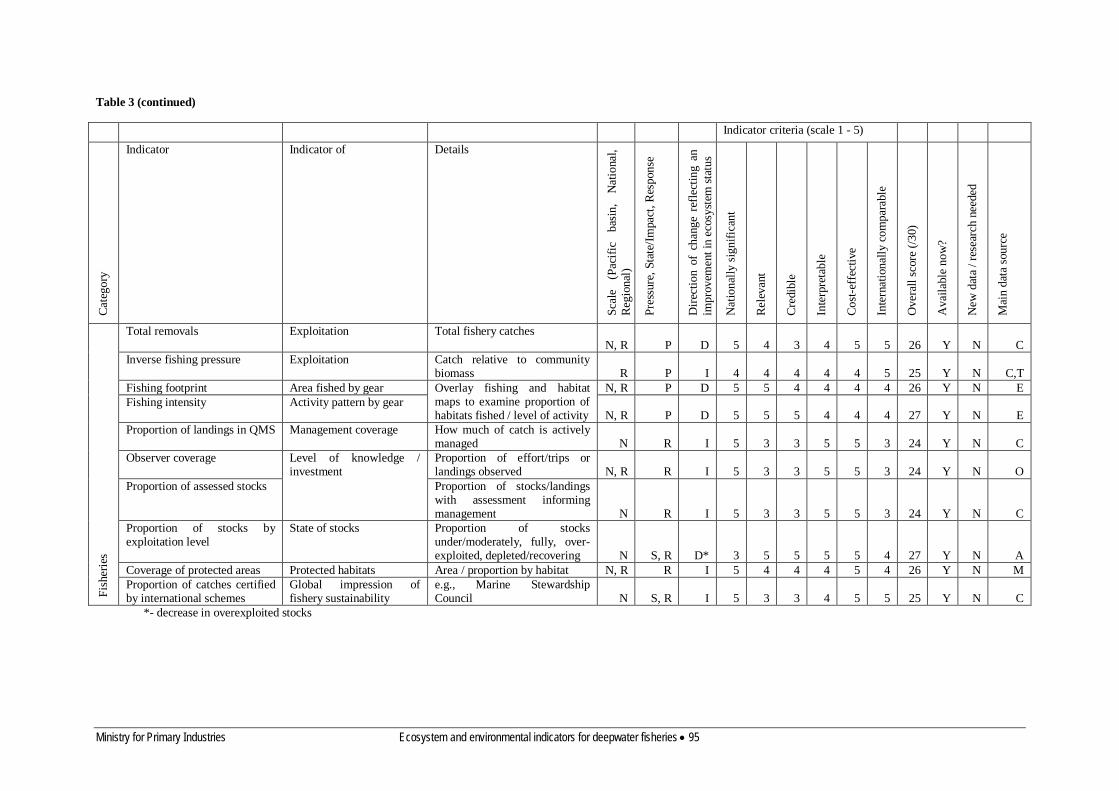
Ministry for Primary Industries Ecosystem and environmental indicators for deepwater fisheries • 95
Table 3 (continued)
*- decrease in overexploited stocks
Indicator criteria (scale 1 - 5)
Cat
egor
y
Indicator Indicator of Details
Scal
e (P
acifi
c ba
sin,
N
atio
nal,
Reg
iona
l)
Pres
sure
, Sta
te/Im
pact
, Res
pons
e
Dire
ctio
n of
cha
nge
refle
ctin
g an
im
prov
emen
t in
ecos
yste
m st
atus
Nat
iona
lly si
gnifi
cant
Rel
evan
t
Cre
dibl
e
Inte
rpre
tabl
e
Cos
t-eff
ectiv
e
Inte
rnat
iona
lly c
ompa
rabl
e
Ove
rall
scor
e (/3
0)
Ava
ilabl
e no
w?
New
dat
a / r
esea
rch
need
ed
Mai
n da
ta s
ourc
e
Fish
erie
s
Total removals Exploitation Total fishery catches N, R P D 5 4 3 4 5 5 26 Y N C
Inverse fishing pressure Exploitation Catch relative to community biomass R P I 4 4 4 4 4 5 25 Y N C,T
Fishing footprint Area fished by gear Overlay fishing and habitat maps to examine proportion of habitats fished / level of activity
N, R P D 5 5 4 4 4 4 26 Y N E Fishing intensity Activity pattern by gear
N, R P D 5 5 5 4 4 4 27 Y N E Proportion of landings in QMS Management coverage How much of catch is actively
managed N R I 5 3 3 5 5 3 24 Y N C Observer coverage Level of knowledge /
investment Proportion of effort/trips or landings observed N, R R I 5 3 3 5 5 3 24 Y N O
Proportion of assessed stocks Proportion of stocks/landings with assessment informing management N R I 5 3 3 5 5 3 24 Y N C
Proportion of stocks by exploitation level
State of stocks Proportion of stocks under/moderately, fully, over-exploited, depleted/recovering N S, R D* 3 5 5 5 5 4 27 Y N A
Coverage of protected areas Protected habitats Area / proportion by habitat N, R R I 5 4 4 4 5 4 26 Y N M Proportion of catches certified by international schemes
Global impression of fishery sustainability
e.g., Marine Stewardship Council N S, R I 5 3 3 4 5 5 25 Y N C

96 • Ecosystem and environmental indicators for deepwater fisheries Ministry for Primary Industries
Table 3 (continued)
Indicator criteria (scale 1 - 5)
Cat
egor
y
Indicator Indicator of Details
Scal
e (P
acifi
c ba
sin,
N
atio
nal,
Reg
iona
l)
Pres
sure
, Sta
te/Im
pact
, Res
pons
e
Dire
ctio
n of
cha
nge
refle
ctin
g an
im
prov
emen
t in
ecos
yste
m st
atus
Nat
iona
lly si
gnifi
cant
Rel
evan
t
Cre
dibl
e
Inte
rpre
tabl
e
Cos
t-eff
ectiv
e
Inte
rnat
iona
lly c
ompa
rabl
e
Ove
rall
scor
e (/3
0)
Ava
ilabl
e no
w?
New
dat
a / r
esea
rch
need
ed
Mai
n da
ta s
ourc
e
Fish
com
mun
ity
Target species biomass Population size Target species biomass (or proportion of total) R S I 4 4 4 5 5 5 27 Y N T
Species distribution Range contraction % of area over which 90% of biomass occurs R S I 3 4 3 4 5 4 23 Y N T
Total biomass Total community biomass
Total survey biomass R S I 3 4 3 5 5 5 25 Y N T
Community biomass ratios Community structure Biomass of specific groups (demersal, key prey, vulnerable species), or proportion of total R S U 3 3 3 3 5 5 22 Y N T
Community diversity Range of measures available – evaluation in relation to patterns in fishing recommended R S U 3 3 3 2 5 5 21 Y Y T
Proportion of large fish Size structure of overall fish community
Proportion of fish above defined size R S I 4 4 4 4 5 5 26 Y N T
Size spectra Slope of size spectra – rate of decline of abundance with size R S D 4 4 4 3 5 5 25 Y N T
Mean trophic level Trophic structure of overall fish community
Mean trophic level of fish community R S I 4 4 3 4 5 5 25 Y N T
Trophic biomass ratios Biomass of specific trophic groups (piscavores, planktivores), or proportion of total R S U 4 4 3 4 5 5 25 Y N T

Ministry for Primary Industries Ecosystem and environmental indicators for deepwater fisheries • 97
Table 3 (continued)
Indicator criteria (scale 1 - 5)
Cat
egor
y
Indicator Indicator of Details
Scal
e (P
acifi
c ba
sin,
N
atio
nal,
Reg
iona
l)
Pres
sure
, Sta
te/Im
pact
, Res
pons
e
Dire
ctio
n of
cha
nge
refle
ctin
g an
im
prov
emen
t in
ecos
yste
m st
atus
Nat
iona
lly si
gnifi
cant
Rel
evan
t
Cre
dibl
e
Inte
rpre
tabl
e
Cos
t-eff
ectiv
e
Inte
rnat
iona
lly c
ompa
rabl
e
Ove
rall
scor
e (/3
0)
Ava
ilabl
e no
w?
New
dat
a / r
esea
rch
need
ed
Mai
n da
ta s
ourc
e
Ben
thic
com
mun
ity
Estimated biomass or production relative to unfished conditions
Physical impact Fishing effect on benthos
R S I 5 3 3 3 4 4 22 Y Y E,O Fishing disturbance relative to natural disturbance
Physical impact Relative magnitude of fishing effect relative to natural disturbance R P D 5 3 2 3 4 3 20 N Y E
Community diversity Community structure Range of measures available – evaluation in relation to patterns in fishing recommended R S U 4 3 3 3 3 3 19 Y Y O
Community and habitat vulnerability
Sensitivity to fishing disturbance
Relative sensitivity of community or habitat. Can be used to track changes over space or time in relation to fishing R S U 4 3 3 3 3 3 19 N Y E,O
Coral distribution Sensitive habitat Distribution of protected deepwater corals N,R S I 4 4 4 4 5 4 25 Y N O
Coral bycatch Fishery interactions Spatial and temporal patterns in coral bycatch N,R P D 4 4 4 4 5 4 25 Y N O
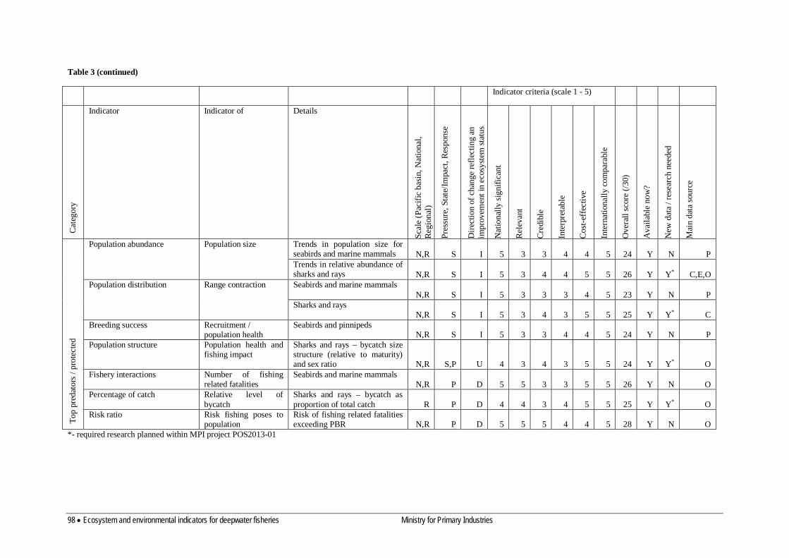
98 • Ecosystem and environmental indicators for deepwater fisheries Ministry for Primary Industries
Table 3 (continued)
Indicator criteria (scale 1 - 5)
Cat
egor
y
Indicator Indicator of Details
Scal
e (P
acifi
c ba
sin,
Nat
iona
l, R
egio
nal)
Pres
sure
, Sta
te/Im
pact
, Res
pons
e
Dire
ctio
n of
cha
nge
refle
ctin
g an
im
prov
emen
t in
ecos
yste
m st
atus
Nat
iona
lly si
gnifi
cant
Rel
evan
t
Cre
dibl
e
Inte
rpre
tabl
e
Cos
t-eff
ectiv
e
Inte
rnat
iona
lly c
ompa
rabl
e
Ove
rall
scor
e (/3
0)
Ava
ilabl
e no
w?
New
dat
a / r
esea
rch
need
ed
Mai
n da
ta s
ourc
e
Top
pred
ator
s / p
rote
cted
Population abundance Population size Trends in population size for seabirds and marine mammals N,R S I 5 3 3 4 4 5 24 Y N P Trends in relative abundance of sharks and rays N,R S I 5 3 4 4 5 5 26 Y Y* C,E,O
Population distribution Range contraction Seabirds and marine mammals N,R S I 5 3 3 3 4 5 23 Y N P
Sharks and rays N,R S I 5 3 4 3 5 5 25 Y Y* C
Breeding success Recruitment / population health
Seabirds and pinnipeds N,R S I 5 3 3 4 4 5 24 Y N P
Population structure Population health and fishing impact
Sharks and rays – bycatch size structure (relative to maturity) and sex ratio N,R S,P U 4 3 4 3 5 5 24 Y Y* O
Fishery interactions Number of fishing related fatalities
Seabirds and marine mammals N,R P D 5 5 3 3 5 5 26 Y N O
Percentage of catch Relative level of bycatch
Sharks and rays – bycatch as proportion of total catch R P D 4 4 3 4 5 5 25 Y Y* O
Risk ratio Risk fishing poses to population
Risk of fishing related fatalities exceeding PBR N,R P D 5 5 5 4 4 5 28 Y N O
*- required research planned within MPI project POS2013-01

Ministry for Primary Industries Ecosystem and environmental indicators for deepwater fisheries • 99
14 ACKNOWLEDGMENTS This work was completed under Ministry for Primary Industries project DEE201005A with co-funding from NIWA under Coasts and Oceans Research Programme 2 (2012/13 SCI). The authors discussed various aspects of the report with staff from the Department of Conservation and the MPI Observer Team, and the final report also benefitted from discussion and feedback from MPI and the Aquatic Environment Working group. The final report was reviewed by Verena Trenkel (IFREMER) and Malcolm Clark.
15 REFERENCES Abraham, E.R.; Thompson, F.N. (2011). Summary of the capture of seabirds, marine mammals, and turtles in New Zealand commercial fisheries, 1998–99 to 2008–09. Final Research Report prepared for Ministry of Fisheries project PRO2007/01. 170 p. (Unpublished report held by the Ministry of Fisheries, Wellington.) Adey, J.M.; Smith, I.P.; Atkinson, R.J.A.; Tuck, I.D.; Taylor, A.C. (2008). 'Ghost fishing' of target and non-target species by Norway lobster Nephrops norvegicus creels. Marine Ecology-Progress Series 366: 119-127. Aebischer, N.J.; Coulson, J.C.; Colebrook, J.M. (1990). Parallel long-term trends across four marine trophic levels and weather. Nature 347: 753-755. Agnew, D. (1997). The CCAMLR Ecosystem Monitoring Programme. Antarctic Science 9: 235-242. Aiken, J.; Moore, G.F.; Trees, C.C.C.C.; Hooker, S.B.; Clarke, D.K.D.K. (1995). The SeaWiFS CZCS-type pigment algorithm. SeaWiFS Technical Report Series NANASA Technical Memorandum 104566 34 p. Ainley, D. (2002). The Ross Sea, Antarctica, where all ecosystem processes still remain for study, but maybe not for long. Marine Ornithology 30: 55-62. Allan, R.J.; Lindesay, J.A.; Parker, D.E. (1996). El Niño Southern Oscillation and Climatic Variability. CSIRO Publications. 405 p. Anderson, C.N.K.; Hsieh, C.; Sandin, S.A.; Hewitt, R.; Hollowed, A.; Beddington, J.; May, R.M.; Sugihara, G. (2008). Why fishing magnifies fluctuations in fish abundance. Nature 452: 835–839. Anderson, O.F. (2006). Review of the historical biological data for orange roughy collected by the MFish observer programme and other sources, and the use of these data in stock assessments. New Zealand Fisheries Assessment Report 2006/14: 41. Anderson, O.F. (2012). Fish and invertebrate bycatch and discards in New Zealand scampi fisheries from 1990–91 until 2009–10. New Zealand Aquatic Environment and Biodiversity Report 100: 65.

100 • Ecosystem and environmental indicators for deepwater fisheries Ministry for Primary Industries
Anderson, O.F.; Doonan, I. (2010). Analysis of CPUE and observer length data in the Pukaki Rise black oreo fishery (OEO 6) from 1980–81 to 2008–09. New Zealand Fisheries Assessment Report 2010/40. Anderson, P.J.; Piatt, J.F. (1999). Community reorganization in the Gulf of Alaska following ocean climate regime shift. Marine Ecology Progress Series 189: 117-123. Antoine, D.; Morel, A. (1996a). Oceanic primary production 1: Adaptation of a spectral light-photosynthesis model in view of application to satellite chlorophyll observations. Global Biogeochemical Cycles 10: 43-55. Antoine, D.; Morel, A. (1996b). Oceanic primary production 2: Estimation of global scale from satellite (Coastal Zone Color Scanner) chlorophyll. Global Biogeochemical Cycles 10: 57-69. Arrigo, K. (2005). Marine microorganisms and global nutrient cycles. Nature 437: 349-355. Atkinson, L.J.; Leslie, R.W.; Field, J.G.; Jarre, A. (2011). Changes in demersal fish assemblages on the west coast of South Africa, 1986-2009. African Journal of Marine Science 33: 157-170. Attrill, M.J.; Power, A.J. (2002). Climatic influence on a marine fish assemblage. Nature 417: 275-278. Ault, J.S.; Smith, S.G.; Bohnsack, J.A. (2005). Evaluation of average length as an estimator of exploitation status for the Florida coral-reef fish community. ICES Journal of Marine Science 62: 417–423. Baird, S.J. (2009). Provision of a Chatham Rise subset of the benthic-optimised marine environemnt classification (BOMEC) created for ther New Zealand 200 n.mile EEZ. NIWA Client Report VSJ10301. p. Baird, S.J.; Tracey, D.; Mormede, S.; Clark, M. (2013). The distribution of protected corals in New Zealand waters (DOC12303 / POP2011-06). NIWA Client Report prepared for Marine Conservation Services (CSP) Department of Conservation WLG2012-43. 93 p. (NIWA Client Report prepared for Marine Conservation Services (CSP) Department of Conservation) Baird, S.J.; Wood, B.; Bagley, N. (2011). Nature and extent of commercial fishing effort on or near the seafloor within the New Zealand 200 n. mile Exclusive Economic Zone. New Zealand Aquatic Environment and Biodiversity Report 73: 50p. Baker, A.N. (1983). Whales and Dolphins of New Zealand and Australia: An Identification Guide. Victoria University Press, Baker, C.S.; Chilvers, B.L.; Constantine, R.; DuFresne, S.; Mattlin, R.H.; van Helden, A.; Hitchmough, R. (2010). Conservation status of New Zealand marine mammals (suborders Cetacea and Pinnipedia), 2009. New Zealand Journal of Marine and Freshwater Research 44(2): 101-115. <http://dx.doi.org/10.1080/00288330.2010.482970>

Ministry for Primary Industries Ecosystem and environmental indicators for deepwater fisheries • 101
Baker, G.B.; Jensz, K.; Chilvers, L. (2012). Aerial survey of New Zealand sea lions - Auckland Islands. Final Research Report for Ministry of Agriculture & Forestry, Deepwater Group & Department of Conservation research project DOCDM-872849. 10 p. Baker, G.B.; Jensz, K.; Cunningham, R. (2013). White-capped albatross population estimate — 2011/12 and 2012/13. Department of Conservation Contract 4431 & Project POP2012-05. p. (Report prepared for Department of Conservation) Bakun, A. (2005). Regime shifts. In: Robinson, A.R.; Brink, K. (eds). The Sea, Vol. 13, The Global Coastal Ocean, Multiscale Interdisciplinary Processes, pp. 971-1026. Harvard University Press, Cambridge, MA, USA. Balch, W.M.; Holligan, P.M.; Ackleson, S.G.; Voss, K.J. (1991). Biological and optical properties of mesoscale coccolithophore blooms in the Gulf of Maine. Limnology and Oceanography 36: 629-643. Ballion, S.; Hamel, J.-F.; Wareham, V.E.; Mercier, A. (2012). "Deep cold-water corals as nurseries for fish larvae." Presented at the International Deep-Sea Coral Symposium, Amsterdam, The Netherlands. Banse, K. (1995). Zooplankton—pivotal role in the control of ocean production. ICES Journal of Marine Science 52: 265-277. Basher, R.E.; Thompson, C.S. (1996). Relationship of air temperatures in New Zealand to regional anomolies in sea-surface temperatureand atmospheric circulation. International Journal of Climatology 16(4): 405-425. <http://dx.doi.org/10.1002/(SICI)1097-0088(199604)16:4<405::AID-JOC14>3.0.CO;2-T> Beaugrand, G. (2004). The North Sea regime shift: Evidence, cause, mechanisms and consequences. Progress in Oceanography 60(2-4): 245-262. Beaugrand, G. (2005). Monitoring pelagic ecosystems using plankton indicators. ICES Journal of Marine Science 62: 333-338. Beaugrand, G.; Brander, K.M.; Lindley, J.A.; Souissi, S.; Reid, P.C. (2003). Plankton have an effect on cod recruitment in North Sea. Nature 426: 661-664. Beaugrand, G.; Edwards, M.; Brander, K.M.; Luczak, C.; Ibanez, F. (2008). Causes and projections of abrupt climate-driven ecosystem shifts in the North Atlantic. Ecology Letters 11: 1157-1168. Beaugrand, G.; Reid, P.C.; Ibanez, F.; Lindley, J.A.; Edwards, M. (2002). Reorganisation of North Atlantic marine copepod biodiversity and climate. Science 296: 1692-1694. Beentjes, M.; Renwick, J. (2001). The Relationship between Red Cod, Pseudophycis Bachus, Recruitment and Environmental Variables in New Zealand. Environmental Biology of Fishes 61(3): 315-328. <http://dx.doi.org/10.1023/A:1010943906264> Begg, G.A.; Hare, J.A.; Sheehan, D.D. (1999). The role of life history parameters as indicators of stock structure. Fisheries Research 43: 141-163.

102 • Ecosystem and environmental indicators for deepwater fisheries Ministry for Primary Industries
Behrenfeld, M.J.; Boss, E.; Siegel, D.A.; Shea, D.M. (2005). Carbon-based ocean productivity and phytoplankton physiology from space. Global Biogeochemical Cycles 19(1): GB1006. <http://dx.doi.org/10.1029/2004GB002299> Behrenfeld, M.J.; Falkowski, P.G. (1997a). A consumer’s guide to phytoplankton primary productivity models. Limnology and Oceanography 42: 1479-1491. Behrenfeld, M.J.; Falkowski, P.G. (1997b). Photosynthetic rates derived from satellite-based chlorophyll concentration. Limnology and Oceanography 42: 1-20. Bell, E. (2013). Identification of seabirds captured in NZ fisheries: 2011/12. DOC Marine Conservation Series. 40p p. (Report prepared for Department of Conservation) Bertrand, S.; Burgos, J.M.; Gerlotto, F.; Atiquipa, J. (2005). Levy trajectories of Peruvian purse-seiners as an indicator of the spatial distribution of anchovy (Engraulis ringens). ICES Journal of Marine Science 62: 477-482. Black, J.; Wood, R.; Berthelsen, T.; Tilney, R. (2013). Monitoring New Zealand’s trawl footprint for deepwater fisheries: 1989–1990 to 2009–2010. . New Zealand Aquatic Environment and Biodiversity Report 110: 57p. Blair, D. (1998). The Kirchhofer technique of synoptic typing revisited. International Journal of Climatology 18(14): 1625-1635. <http://dx.doi.org/10.1002/(SICI)1097-0088(19981130)18:14<1625::AID-JOC330>3.0.CO;2-B> Blanchard, F.; Boucher, J. (2001). Temporal variability of total biomass in harvested communities of demersal fishes. Fisheries Research 49: 283-293. Blanchard, J.L.; Coll, M.; Trenkel, V.M.; Vergnon, R.; Yemane, D.; Jouffre, D.; Link, J.S.; Shin, Y.-J. (2010). Trend analysis of indicators: a comparison of recent changes in the status of marine ecosystems around the world. ICES Journal of Marine Science: Journal du Conseil 67(4): 732-744. <http://dx.doi.org/10.1093/icesjms/fsp282> Blanchard, J.L.; Dulvy, N.K.; Jennings, S.; Ellis, J.R.; Pinnegar, J.K.; Tidd, A.; Kell, L.T. (2005). Do climate and fishing influence size-based indicators of Celtic Sea fish community structure? ICES Journal of Marine Science 62: 405–411. Booth, J.D.; Bradford, E.; Renwick, J.A. (2000). Jasus edwardsii puerulus settlement levels in relation to the ocean environment and to subsequent juvenile and recruit abundance. New Zealand Fisheries Assessment Report 2000/34: 48. Bopp, L.; Monfray, P.; Aumont, O.; Dufresne, J.-L.; Le Treut, H.; Madec, G.; Terray, L.; Orr, J.C. (2001). Potential impact of climate change on marine export production. Global Biogeochemical Cycles 15(1): 81-99. <http://dx.doi.org/10.1029/1999GB001256> Bostock, H.C.; Mikaloff Fletcher, S.E.; Williams, M.J.M. (2013). Estimating carbonate parameters from hydrographic data for the intermediate and deep waters of the Southern Hemisphere Oceans. Biogeosciences Discuss. 10(4): 6225-6257. <http://dx.doi.org/10.5194/bgd-10-6225-2013>

Ministry for Primary Industries Ecosystem and environmental indicators for deepwater fisheries • 103
Boyd, I.L.; Wanless, S.; Camphuysen, C.J. (eds). (2006). Top predators in marine ecosystems: their role in monitoring and management. Conservation Biology. Wiley, Cambridge. 369 p. Boyd, P.; LaRoche, J.; Gall, M.; Frew, R.; McKay, R.M.L. (1999). The role of iron, light and silicate in controlling algal biomass in sub-Antarctic water SE of New Zealand. Journal of Geophysical Research 104(C6): 13395-13408. Boyd, P.W. (2002). The role of iron in the biogeochemistry of the Southern Ocean and equatorial Pacific: a comparison of in situ iron enrichments. Deep Sea Research Part II: Topical Studies in Oceanography 49(9–10): 1803-1821. <http://dx.doi.org/http://dx.doi.org/10.1016/S0967-0645(02)00013-9> Boyd, P.W. (2008). Quantifying the surface-subsurface biogeochemical coupling during the VERTIGO ALOHA and K2 studies. Deep-Sea Research II 55: 1578-1593. Boyer, T.; Levitus, S.; Garcia, H.; Locarnini, R.A.; Stephens, C.; Antonov, J. (2005). Objective analyses of annual, seasonal, and monthly temperature and salinity for the World Ocean on a 0.25° grid. International Journal of Climatology 25(7): 931-945. <http://dx.doi.org/10.1002/joc.1173> Branch, T.A. (2009). How do individual transferable quotas affect marine ecosystems? Fish and Fisheries 10: 39-57. Branch, T.A.; Watson, R.; Fulton, E.A.; Jennings, S.; McGillard, C.R.; Pablico, G.T.; Ricard, D.; Tracey, S.R. (2010). The trophic fingerprint of marine fisheries. Nature 468: 431-435. Brander, K.M. (2004). Cod recruitment is strongly affected by climate when stock biomass is low. ICES Journal of Marine Science 62: 339-343. Brander, K.M. (2010). Impacts of climate change on fisheries. Journal of Marine Systems 79: 389-402. Brierley, A.S.; Kingsford, M.J. (2009). Impacts of climate change on marine organisms and ecosystems. Current Biology 19: R602-R614. Brock, W.A.; Carpenter, S.R. (2006). Variance as a leading indicator of regime shift in ecosystem services. Ecology and Society 11: 9. Buesseler, K.; Boyd, P. (2009). Shedding light on processes that control particle export and flux attenuation in the twilight zone of the open ocean. Limnology and oceanography 54: 1210-1232. Buesseler, K.O.; Lamborg, C.H.; Boyd, P.W.; Lam, P.J.; Trull, T.W.; Bidigare, R.R.; Bishop, J.K.B.; Casciotti, K.L.; Dehairs, F.; Elskens, M.; Honda, M.; Karl, D.M.; Siegel, D.A.; Silver, M.W.; Steinberg, D.K.; Valdes, J.; Van Mooy, B.; Wilson, S. (2007). Revisiting Carbon Flux Through the Ocean's Twilight Zone. Science 316(5824): 567-570. <http://dx.doi.org/10.1126/science.1137959>

104 • Ecosystem and environmental indicators for deepwater fisheries Ministry for Primary Industries
Bull, B.; Livingston, M.E. (2001). Links between climate variation and year class strength of New Zealand hoki (Macruronus novaezelandiae): an update. New Zealand Journal of Marine and Freshwater Research 35: 871-880. Caddy, J.F.; Garibaldi, L. (2000). Apparent changes in the trophic composition of world marine harvests: the perspective from the FAO capture database. Ocean and Coastal Management 43: 615–655. Caldeira, K.; Wickett, M.E. (2003). Anthropogenic carbon and ocean pH. Nature 425: 365. Campbell, J.; Antoine, D.; Armstrong, R.; Arrigo, K.; Balch, W.; Barber, R.; Behrenfeld, M.; Bidigare, R.; Bishop, J.; Carr, M.-E.; Esaias, W.; Falkowski, P.; Hoepffner, N.; Iverson, R.; Kiefer, D.; Lohrenz, S.; Marra, J.; Morel, A.; Ryan, J.; Vedernikov, V.; Waters, K.; Yentsch, C.; Yoder, J. (2002). Comparison of algorithms for estimating ocean primary production from surface chlorophyll, temperature, and irradiance. Global Biogeochemical Cycles 16(3): 9-1-9-15. <http://dx.doi.org/10.1029/2001GB001444> Campbell, N.; Neat, F.; Burns, F.; Kunzlik, P. (2011). Species richness, taxonomic diversity, and taxonomic distinctness of the deep-water demersal fish community on the Northeast Atlantic continental slope (ICES Subdivision VIa). ICES Journal of Marine Science 68: 365-376. CANZ. (1996). Undersea New Zealand (New Zealand Region Physiography) 1:400 000 000 (2nd ed.). New Zealand Oceanographic Institute Chart Miscellaneous Series no. 74. Carpenter, S.R.; Brock, W.A. (2006). Rising variance: A leading indicator of ecological transition. Ecology Letters 9: 311-318. Carr, M.-E.; Friedrichs, M.A.M.; Schmeltz, M.; Noguchi Aita, M.; Antoine, D.; Arrigo, K.R.; Asanuma, I.; Aumont, O.; Barber, R.; Behrenfeld, M.; Bidigare, R.; Buitenhuis, E.T.; Campbell, J.; Ciotti, A.; Dierssen, H.; Dowell, M.; Dunne, J.; Esaias, W.; Gentili, B.; Gregg, W.; Groom, S.; Hoepffner, N.; Ishizaka, J.; Kameda, T.; Le Quéré, C.; Lohrenz, S.; Marra, J.; Mélin, F.; Moore, K.; Morel, A.; Reddy, T.E.; Ryan, J.; Scardi, M.; Smyth, T.; Turpie, K.; Tilstone, G.; Waters, K.; Yamanaka, Y. (2006). A comparison of global estimates of marine primary production from ocean color. Deep Sea Research Part II: Topical Studies in Oceanography 53(5–7): 741-770. <http://dx.doi.org/http://dx.doi.org/10.1016/j.dsr2.2006.01.028> CCAMLR (2004). CCAMLR Ecosystem monitoring programme - Standard methods. 268 p. (Report published by CCAMLR) CGER. (2000). Ecological indicators for the nation. National Acadamy Press, Washington. 180p Chelton, D.B.; Xie, S.P. (2010). Coupled ocean-atmosphere interaction at oceanic mesoscales. Oceanography 23: 52-69. Cheung, W.W.L.; Pitcher, T.J.; Pauly, D. (2005). A fuzzy logic expert system to estimate intrinsic extinction vulnerabilities of marine fishes to fishing. Biological Conservation 124: 97-111.

Ministry for Primary Industries Ecosystem and environmental indicators for deepwater fisheries • 105
Chilvers, L. (2012). Research to assess the demographic parameters of New Zealand sea lions, Auckland Islands. Final Research Report for Conservation Services Programme research project POP2011/01. 10 p. Chiswell, S.M. (1994). Variability in sea surface temperature around New Zealand from AVHRR images. New Zealand Journal of Marine and Freshwater Research 28(2): 179-192. <http://dx.doi.org/10.1080/00288330.1994.9516606> Chiswell, S.M.; Bradford-Grieve, J.; Hadfield, M.G.; Kennan, S.C. (2013). Climatology of surface chlorophyll a, autumn-winter and spring blooms in the southwest Pacific Ocean. Journal of Geophysical Research: Oceans 118(2): 1003-1018. <http://dx.doi.org/10.1002/jgrc.20088> Chiswell, S.M.; Schiel, D.R. (2001). Influence of along‐shore advection and upwelling on coastal temperature at Kaikoura Peninsula, New Zealand. New Zealand Journal of Marine and Freshwater Research 35(2): 307-317. <http://dx.doi.org/10.1080/00288330.2001.9517000> Clark, M. (1985). The food and feeding of seven fish species from the Campbell Plateau, New Zealand. New Zealand Journal of Marine and Freshwater Research 19: 339-363. Clark, M.; King, K.J.; McMillan, P.J. (1989). The food and feeding relationships of black oreo, Allocyttus niger, smooth oreo, Pseudocyttus maculates, and eight other fish species from the continental slope of the south-west Chatham Rise, New Zealand. Journal of Fish Biology 35: 465-484. Clark, M.R.; Rowden, A.A. (2009). Effect of deepwater trawling on the macro-invertebrate assemblages of seamounts on the Chatham Rise, New Zealand. Deep Sea Research Part I: Oceanographic Research Papers 56(9): 1540-1554. <http://dx.doi.org/http://dx.doi.org/10.1016/j.dsr.2009.04.015> Clark, M.R.; Tittensor, D.P. (2010). An index to assess the risk to stony corals from bottom trawling on seamounts. Marine Ecology 31: 200-211. <http://dx.doi.org/10.1111/j.1439-0485.2010.00392.x> Clark, M.R.; Watling, L.; Rowden, A.A.; Guinotte, J.M.; Smith, C.R. (2011). A global seamount classification to aid the scientific design of marine protected area networks. Ocean & Coastal Management 54(1): 19-36. <http://dx.doi.org/http://dx.doi.org/10.1016/j.ocecoaman.2010.10.006> Clarke, K.R.; Warwick, R.M. (1999). The taxonomic distinctness measure of biodiversity: weighting of step lengths between hierarchical levels. Marine Ecology Progress Series 184: 21-29. Clarke, S.; Francis, M.P.; Griggs, L. (2013). Review of shark meat markets, discard mortality and pelagic shark data availability, and a proposal for a shark indicator analysis. New Zealand Fisheries Assessment Report 2013/65: 74p.

106 • Ecosystem and environmental indicators for deepwater fisheries Ministry for Primary Industries
Clarke, S.; Harley, S.; Hoyle, S.; Rice, J. (2011). An indicator-based analysis of key shark species based on data held by SPC-OFP. Western Central Pacific Fisheries Commission Scientific Committee sevents regular session SC7-EB-WP-01: 88p. Coll, M.; Libralato, S.; Tudela, S.; Palomera, I.; Pranovi, F. (2008). Ecosystem Overfishing in the Ocean. PLoS ONE 3(12): e3881. <http://dx.doi.org/10.1371/journal.pone.0003881> Comiso, J.C.; McClain, C.R.; Sulivan, C.W.; Ryan, J.P.; Leonard, C.L. (1993). Coastal Zone Color Scanner pigment concentrations in the Southern Ocean and relationships to geophysical features. Journal of Geophysical Research 98: 2419-2451. Connell, A.; Dunn, M.R.; J., F. (2010). Diet and dietary variation in the hoki Macruronus novaezelandiae. New Zealand Journal of Marine and Freshwater Research 44: 289-308. Constable, A.J. (2006). Setting management goals using information from predators. In: Boyd, I.L.; Wanless, S.; Camphuysen, C.J. (eds). Top predators in marine ecosystems: their role in monitoring and management, pp. 324-346. Conservation Biology 12. Cambridge University Press, Cooley, S.R.; Doney, S.C. (2009a). Anticipating ocean acidification's economic consequences for commercial fisheries. Environmental Research Letters 4: 1-18. Cooley, S.R.; Doney, S.C. (2009b). Ocean acidification’s impact on fisheries and societies--- a U.S. perspective. Current: the Journal of Marine Education 25: 15-19. Cotter, J.; Mesnil, B.; Witthames, P.; Parker-Humphreys, M. (2009). Notes on nine biological indicators estimable from trawl surveys with an illustrative assessment for North Sea cod. Aquatic Living Resources 22(02): 135-153. <http://dx.doi.org/doi:10.1051/alr/2009016> Cox, P.M.; Betts, R.A.; Jones, C.D.; Spall, S.A.; Totterdell, I.J. (2000). Acceleration of global warming due to carbon-cycle feedbacks in a coupled climate model. Nature 408: 184-187. Cryer, M.; Hartill, B.; O'Shea, S. (2002). Modification of marine benthos by trawling: Toward a generalization for the deep ocean? Ecological Applications 12(6): 1824–1839. Currie, K.; Hunter, K. (1999). Seasonal variation of surface water CO2 partial pressure in the Southland Current, east of New Zealand. Marine and Freshwater Research 50: 375-382. Currie, K.; Reid, M.; Hunter, K. (2011). Interannual variability of carbon dioxide drawdown by subantarctic surface water near New Zealand. Biogeochemistry 104: 23-24. Cury, P.; Shannon, L.J.; Roux, J.P.; Daskalov, G.M.; Jarre, A.; Moloney, C.L.; Pauly, D. (2005). Trophodynamic indicators for an ecosystem approach to fisheries. ICES Journal of Marine Science 62: 430–442. Cury, P.M.; Christensen, V. (2005). Quantitative ecosystem indicators for fisheries management. ICES Journal of Marine Science 62(3): 307–310.

Ministry for Primary Industries Ecosystem and environmental indicators for deepwater fisheries • 107
D'Onghia, G.; Maiorano, P.; Carlucci, R.; Capezzuto, F.; Carluccio, A.; Tursi, A.; Sion, L. (2012). Comparing Deep-Sea Fish Fauna between Coral and Non-Coral “Megahabitats” in the Santa Maria di Leuca Cold-Water Coral Province (Mediterranean Sea). PLoS ONE 7(9): e44509. <http://dx.doi.org/10.1371/journal.pone.0044509> D’Onghia, G.; Maiorano, P.; Sion, L.; Giove, A.; Capezzuto, F.; Carlucci, R.; Tursi, A. (2010). Effects of deep-water coral banks on the abundance and size structure of the megafauna in the Mediterranean Sea. Deep Sea Research Part II: Topical Studies in Oceanography 57(5–6): 397-411. <http://dx.doi.org/http://dx.doi.org/10.1016/j.dsr2.2009.08.022> Daskalov, G.M.; Grishin, A.N.; Rodionov, S.; Mihneva, V. (2007). Trophic cascades triggered by overfishing reveal possible mechanisms of ecosystem regime shifts. Proceedings of the National Academy of Sciences 104: 10518. de Juan, S.; Demestre, M.; Thrush, S.F. (2009). Defining ecological indicators of trawling disturbance when everywhere that can be fished is fished: a Mediterranean case study. Marine Policy 33: 472-478. Diaz, R.J.; Rosenberg, R. (2008). Spreading Dead Zones and Consequences for Marine Ecosystems. Science 321(5891): 926-929. <http://dx.doi.org/10.1126/science.1156401> Diesing, M.; Stephens, D.; Aldridge, J. (2013). A proposed method for assessing the extent of the seabed significantly affected by demersal fishing in the Greater North Sea. ICES Journal of Marine Science: Journal du Conseil 70(6): 1085-1096. <http://dx.doi.org/10.1093/icesjms/fst066> Diggle, P.J.; Menezes, R.; Su, T.-l. (2010). Geostatistical inference under preferential sampling. Journal of the Royal Statistical Society: Series C (Applied Statistics) 59(2): 191-232. <http://dx.doi.org/10.1111/j.1467-9876.2009.00701.x> Drinkwater, K.F. (2006). The regime shift of the 1920s and 1930s in the North Atlantic. Progress in Oceanography 68: 134-151. Dugdale, R.; Goering, J. (1967). Uptake of new and regenerated forms of nitrogen in new production. Limnology and Oceanography 12: 196-206. Dunn, J.R.; Ridgway, K.R. (2002). Mapping ocean properties in regions of complex topography. Deep Sea Research Part I: Oceanographic Research Papers 49(3): 591-604. <http://dx.doi.org/http://dx.doi.org/10.1016/S0967-0637(01)00069-3> Dunn, M.R.; Connell, A.M.; Forman, J.; Stevens, D.W.; Horn, P.L. (2010a). Diet of Two Large Sympatric Teleosts, the Ling (Genypterus blacodes) and Hake (Merluccius australis). Plos One 5(10). <http://dx.doi.org/e13647 10.1371/journal.pone.0013647> Dunn, M.R.; Griggs, L.; Forman, J.; Horn, P. (2010b). Feeding habits and niche separation among the deep-sea chimaeroid fishes Harriotta raleighana, Hydrolagus bemisi and Hydrolagus novaezealandiae. Marine Ecology Progress Series 407: 209-225.

108 • Ecosystem and environmental indicators for deepwater fisheries Ministry for Primary Industries
Dunn, M.R.; Horn, P.; Connell, A.; Stevens, D.W.; Forman, J.; Pinkerton, M.H.; Griggs, L.; Notman, P.; Wood, P. (2009a). Ecosystem-scale trophic relationships: diet composition and guild structure of middle-depths fish on the Chatham Rise. Final Research Report for Ministry of Fisheries research project ZBD2004-02. p. (Unpublished report held by MFish, Wellington.) Dunn, M.R.; Hurst, R.; Renwick, J.A.; Francis, R.I.C.C.; Devine, J.; McKenzie, A. (2009b). Fish abundance and climate trends in New Zealand. New Zealand Aquatic Environment and Biodiversity Report 31: 74pp. Dunn, M.R.; Stevens, D.W.; Forman, J.S.; Connell, A. (2013). Trophic Interactions and Distribution of Some Squaliforme Sharks, Including New Diet Descriptions for <italic>Deania calcea</italic> and <italic>Squalus acanthias</italic>. PLoS ONE 8(3): e59938. <http://dx.doi.org/10.1371/journal.pone.0059938> Dunne, J.P.; Armstrong, R.A.; Gnanadesikan, A.; Sarmiento, J.L. (2005). Empirical and mechanistic models for the particle export ratio. Global Biogeochemical Cycles 19(4): GB4026. <http://dx.doi.org/10.1029/2004GB002390> Duplisea, D.E.; Castonguay, M. (2006). Comparison and utility of different size-based metrics of fish communities for detecting fishery impacts. Canadian Journal of Fisheries and Aquatic Sciences 63: 810–820. Duplisea, D.E.; Kerr, S.R.; Dickie, L.M. (1997). Demersal fish biomass size spectra on the Scotian Shelf, Canada: species replacement at a shelfwide scale. Canadian Journal of Fisheries and Aquatic Science 54(1725-1735). Eleftheriou, A. (2000). Marine benthos dynamics: Environmental and fisheries impacts - Introduction and overview. ICES Journal of Marine Science 57(5): 1299–1302. Emery, W.J.; Thomson, R.E. (1997). Data Analysis Methods in Physical Oceanography. Pergamon, Oxford. Eppley, R.W. (1972). Temperature and phytoplankton growth in the sea. Fishery Bulletin 70: 1063-1085. Fabry, V.J.; Seibel, B.A.; Feely, R.A.; Orr, J.C. (2008). Impacts of ocean acidification on marine fauna and ecosystem processes. ICES Journal of Marine Science 65: 414-432. Fanning, K. (1989). Influence of atmospheric pollution on nutrient limitation in the ocean. Nature 339: 460-463. Fasham, M.J.R.; Baliño, B.M.; Bowles, M.C. (eds). (2001). A new vision of ocean biogeochemistry after a decade of the Joint Global Ocean Flux Study (JGOFS). Ambio Special report 10. 4-31 p. Fautin, D.F.; Eash-Loucks, T. (2012). "Oxygen-minimum zones: a threat to deep-sea corals and other cnidarians?" Presented at the 5th International Symposium on Deep-Sea Corals.

Ministry for Primary Industries Ecosystem and environmental indicators for deepwater fisheries • 109
Feely, R.A.; Sabine, C.L.; Byrne, R.H.; Millero, F.J.; Dickson, A.G.; Wanninkhof, R.; Murata, A.; Miller, L.A.; Greeley, D. (2012). Decadal changes in the aragonite and calcite saturation state of the Pacific Ocean. Global Biogeochemical Cycles 26(3): GB3001. <http://dx.doi.org/10.1029/2011GB004157> Feely, R.A.; Sabine, C.L.; Lee, K.; Berelson, W.; Kleypas, J.; Fabry, V.J.; Millero, F.J. (2004). Impact of Anthropogenic CO2 on the CaCO3 System in the Oceans. Science 305(5682): 362-366. <http://dx.doi.org/10.1126/science.1097329> Fillipi, D.; Waugh, S.; Nichol, S. (2010). Revised spatial indicators for seabird interactions with longline fisheries in the western and central pacific. 47 p. Unpublished report (WCPFC-SC6-2010-EB-IP-01) prepared for the Western and Central Pacific Fisheries Commission. Fisher, J.A.D.; Frank, K.T. (2004). Abundance-distribution relationships and conservation of exploited marine fishes. Marine Ecology Progress Series 279: 201–213. Flint, E. (1999). Status of seabird populations and conservation in the tropical island pacific. In: Eldredge, L.G.; Maragos, J.E.; Holthus, P.F.; Takeuchi, H.F. (eds). Marine and coastal biodiversity in the tropical island pacific region. 2 Population, development and conservation priorities, pp. 189-210. East-West Centre, Fogarty, M.J.; Murawski, S.A. (1998). Large-scale disturbance and the structure of marine system: Fishery impacts on Georges Bank. Ecological Applications 8(1): S6-S22. Francis, M.P. (1994a). Duration of larval and spawning periods in Pagrus auratus (Sparidae) determined from otolith daily increments. Environmental Biology of Fishes 39: 137-152. Francis, M.P. (1994b). Growth of juvenile snapper, Pagurus auratus. New Zealand Journal of Marine and Freshwater Research 28: 201 -218. Francis, R.C.; Hare, S.R. (1994). Decadal scale regime shifts in large marine ecosystems of the northeast Pacific: A case for historical science. Fisheries Oceanography 3: 279-291. Francis, R.C.; Hare, S.R.; Hollowed, A.B.; Wooster, W.S. (1998). Effects of interdecadal climate variability on the oceanic ecosystems of the NE Pacific. Fisheries Oceanography 7(1): 1-21. <http://dx.doi.org/10.1046/j.1365-2419.1998.00052.x> Francis, R.I.C.C. (2006). Measuring the strength of environment-recruitment relationships: the importance of including predictor screening within cross-validations. ICES Journal of Marine Science 63: 594-599. Frank, K.T.; Petrie, B.; Shackell, N.L. (2007). The ups and downs of trophic control in continental shelf ecosystems. Trends in Ecology & Evolution 22: 237-242. Freeman, D.J.; Marshall, B.A.; Ahyong, S.T.; Wing, S.R.; Hitchmough, R.A. (2010). Conservation status of New Zealand marine invertebrates, 2009. New Zealand Journal of Marine and Freshwater Research 44(3): 129-148. <http://dx.doi.org/10.1080/00288330.2010.495373>

110 • Ecosystem and environmental indicators for deepwater fisheries Ministry for Primary Industries
Freon, P.; Drapeau, L.; David, J.H.M.; Fernandez Moreno, A.; Leslie, R.W.; Oosthuizen, W.H.; Shannon, L.J.; van der Lingen, C.D. (2005). Spatialized ecosystem indicators in the southern Benguela. ICES Journal of Marine Science 62(3): 459–468. Friedland, K.D.; Stock, C.; Drinkwater, K.F.; Link, J.S.; Leaf, R.T.; Shank, B.V.; Rose, J.M.; Pilskaln, C.H.; Fogarty, M.J. (2012). Pathways between Primary Production and Fisheries Yields of Large Marine Ecosystems. PLoS ONE 7(1): e28945. <http://dx.doi.org/10.1371/journal.pone.0028945> Frouin, R.; Franz, B.; Wang, M. (2003a). Algorithm to estimate PAR from SeaWiFS data, Version 1.2 – Documentation. NASA publication, oceancolor.gsfc.nasa.gov/DOCS/seawifs_par_wfigs.pdf. 15 p. Frouin, R.; Franz, B.; Werdell, P. (2003b). The SeaWiFS PAR product. In: Hooker, S.; Firestone, E. (eds). NASA Technical Memorandum 2003-206892, pp. 1-74. NASA Goddard Space Flight Center, Greenbelt, Maryland. Frouin, R.; Murakami, H. (2007). Estimating photosynthetically available radiation at the ocean surface from ADEOS-II global imager data. Journal of Oceanography 63(3): 493-503. <http://dx.doi.org/10.1007/s10872-007-0044-3> Frouin, R.; Pinker, R.T. (1995). Estimating Photosynthetically Active Radiation (PAR) at the earth's surface from satellite observations. Remote Sensing of Environment 51(1): 98-107. <http://dx.doi.org/http://dx.doi.org/10.1016/0034-4257(94)00068-X> Fulton, E.A.; Link, J.S.; Kaplan, I.C.; Savina-Rolland, M.; Johnson, P.; Ainsworth, C.; Horne, P.; Gorton, R.; Gamble, R.J.; Smith, A.D.M.; Smith, D.C. (2011). Lessons in modelling and management of marine ecosystems: the Atlantis experience. Fish and Fisheries 12(2): 171-188. <http://dx.doi.org/10.1111/j.1467-2979.2011.00412.x> Fulton, E.A.; Smith, A.D.M.; Punt, A.E. (2005). Which ecological indicators can robustly detect effects of fishing? ICES Journal of Marine Science 62: 540–551. Fulton, E.A.; Smith, A.D.M.; Webb, H.; Slater, J. (2004). Ecological indicators for the impacts of fishing on non-target species, communities and ecosystems: Review of potential indicators. AFMA Final Research report R99/1546: 119pp. Garcia, S.M.; Staples, D.J. (2000). Sustainability reference systems and indicators for responsible marine capture fisheries: a review of concepts and elements for a set of guidelines. Marine and Freshwater Research 51: 385–426. Garver, S.A.; Siegel, D.A. (1997). Inherent optical property inversion of ocean color spectra and its biogeochemical interpretation: 1. Time series from the Sargasso Sea. Journal of Geophysical Research: Oceans 102(C8): 18607-18625. <http://dx.doi.org/10.1029/96JC03243> Gascuel, D.; Bozec, Y.-M.; Chassot, E.; Colomb, A.; Laurans, M. (2005). The trophic spectrum: theory and application as an ecosystem indicator. ICES Journal of Marine Science 62: 443–452.

Ministry for Primary Industries Ecosystem and environmental indicators for deepwater fisheries • 111
Gass, S.E.; Roberts, J.M. (2006). The occurrence of the cold-water coral Lophelia pertusa (Scleractinia) on oil and gas platforms in the North Sea: colony growth, recruitment and environmental controls on distribution. Marine Pollution Bulletin 52: 549-559. Gattuso, J.-P.; Hansson, L. (2011). Ocean Acidification. Oxford University Press, Oxford, UK. Gazeau, F.; Quiblier, C.; Jansen, J.M.; Gattuso, J.-P.; Middelburg, J.J.; Heip, C.H.R. (2007). Impact of elevated CO2 on shellfish calcification. Geophysical Research Letters 34(7): L07603. <http://dx.doi.org/10.1029/2006GL028554> Gelfand, A.E.; Sahu, S.K.; Holland, D.M. (2012). On the effect of preferential sampling in spatial prediction. Environmetrics 23(7): 565-578. <http://dx.doi.org/10.1002/env.2169> Gerritsen, H.; Lordan, C. (2011). Integrating vessel monitoring systems (VMS) data with daily catch data from logbooks to explore the spatial distribution of catch and effort at high resolution. ICES Journal of Marine Science 68: 245-252. Gilbert, D.J.; Annala, J.H.; Johnston, K. (2000). Technical background to fish stock indicators for state-of-environment reporting in New Zealand. Marine Freshwater Research 51: 451-464. Goni, R. (1998). Ecosystem effects of marine fisheries: an overview. Ocean and Coastal Managment 40: 37-64. Gordon, H.R.; Brown, O.B.; Evans, R.H.; Brown, J.W.; Smith, R.C.; Baker, K.S.; Clark, D.K. (1988). A semianalytic radiance model of ocean color. Journal of Geophysical Research: Atmospheres 93(D9): 10909-10924. <http://dx.doi.org/10.1029/JD093iD09p10909> Greenstreet, S.P.; Hall, S.J. (1996). Fishing and the ground-fish assemblage structure in the north-western North Sea: an analysis of long term and spatial trends. Journal of Animal Ecology 65: 577-598. Greenstreet, S.P.; Rogers, S.I. (2006). Indicators of the health of the North Sea fish community: identifying reference levels for an ecosystem approach to management. ICES Journal of Marine Science 63: 573–593. Greenstreet, S.P.R.; Spence, F.E.; McMillan, J.A. (1999). Fishing effects in northeast Atlantic shelf seas: patterns in fishing effort, diversity and community structure. V. Changes in structure of the North Sea groundfish species assemblage between 1925 and 1996. Fisheries Research 40: 153–183. Gregg, W.W.; Conkright, M.E.; Ginoux, P.; O'Reilly, J.E.; Casey, N.W. (2003). Ocean primary production and climate: Global decadal changes. Geophysical Research Letters 30(15): 1809. <http://dx.doi.org/10.1029/2003GL016889> Griffith, J.A. (1997). Connecting Ecological Monitoring and Ecological Indicators: A Review of the Literature. Journal of Environmental Systems 26: 325-363.
112 • Ecosystem and environmental indicators for deepwater fisheries Ministry for Primary Industries
Guinotte, J.M.; Fabry, V.J. (2008). Ocean Acidification and Its Potential Effects on Marine Ecosystems. Annals of the New York Academy of Sciences 1134(1): 320-342. <http://dx.doi.org/10.1196/annals.1439.013> Guttal, V.; Jayaprakash, C. (2008). Changing skewness: an early warning signal of regime shifts in ecological systems. Ecology Letters 11: 450-460. Halpern, B.S.; Longo, C.; Hardy, D.; McLeod, K.L.; Samhouri, J.F.; Katona, S.K.; Kleisner, K.; Lester, S.E.; O/'Leary, J.; Ranelletti, M.; Rosenberg, A.A.; Scarborough, C.; Selig, E.R.; Best, B.D.; Brumbaugh, D.R.; Chapin, F.S.; Crowder, L.B.; Daly, K.L.; Doney, S.C.; Elfes, C.; Fogarty, M.J.; Gaines, S.D.; Jacobsen, K.I.; Karrer, L.B.; Leslie, H.M.; Neeley, E.; Pauly, D.; Polasky, S.; Ris, B.; St Martin, K.; Stone, G.S.; Sumaila, U.R.; Zeller, D. (2012). An index to assess the health and benefits of the global ocean. Nature 488(7413): 615-620. 10.1038/nature11397 <http://dx.doi.org/http://www.nature.com/nature/journal/v488/n7413/abs/nature11397.html#supplementary-information> Hanchet, S.M.; Renwick, J.A. (1999). Prediction of year class strength in southern blue whiting (Micromesistius australis) in New Zealand waters. New Zealand Fisheries Assessment Report 99/51: 24. Hewitt, J.E.; Julian, K.; Bone, E.K. (2010). Chatham–Challenger Ocean Survey 20/20 Post-Voyage Analyses: Objective 10 – Biotic habitats and their sensitivity to physical disturbance. New Zealand Aquatic Environment and Biodiversity Report 81. Hiddink, J.G.; Jennings, S.; Kaiser, M.J. (2006). Indicators of the Ecological Impact of Bottom-Trawl Disturbance on Seabed Communities. Ecosystems 9: 1190-1199. Hiddink, J.G.; ter Hofstede, R. (2008). Climate induced increases in species richness of marine fishes. Global Change Biology 14: 453-460. Hilborn, R.; Walters, C. (1992). Quantitative fisheries stock assessment: choice, dynamics and uncertainty. Chapman & Hall, New York. 570 pp Hitchmough, R. (2002). New Zealand Threat Classification System lists. Department of Conservation, Threatened Species Occasional Publication 23. 210 p. Hollowed, A.B.; Barange, M.; Beamish, R.J.; Brander, K.; Cochrane, K.; Drinkwater, K.; Foreman, M.G.G.; Hare, J.A.; Holt, J.; Ito, S.-i.; Kim, S.; King, J.R.; Loeng, H.; MacKenzie, B.R.; Mueter, F.J.; Okey, T.A.; Peck, M.A.; Radchenko, V.I.; Rice, J.C.; Schirripa, M.J.; Yatsu, A.; Yamanaka, Y. (2013). Projected impacts of climate change on marine fish and fisheries. ICES Journal of Marine Science: Journal du Conseil. <http://dx.doi.org/10.1093/icesjms/fst081> Hooker, S.B.; Esaias, W.E.; Feldman, G.C.; Greg, W.W.; McClain, C.R. (1992). An overview of SeaWiFS and ocean colour. In: Hooker, S.B.; Firestone, E.R. (eds). NASA Technical Memorandum 104566 (SeaWiFS Technical Report Series), pp. 24. Hooper, D.U.; Chapin, F.S.; Ewel, J.J.; Hector, A.; Inchausti, P.; Lavorel, S.; Lawton, J.H.; Lodge, D.M.; Loreau, M.; Naeem, S.; Schmid, B.; Setälä, H.; Symstad, A.J.; Vandermeer, J.;

Ministry for Primary Industries Ecosystem and environmental indicators for deepwater fisheries • 113
Wardle, D.A. (2005). EFFECTS OF BIODIVERSITY ON ECOSYSTEM FUNCTIONING: A CONSENSUS OF CURRENT KNOWLEDGE. Ecological Monographs 75(1): 3-35. <http://dx.doi.org/10.1890/04-0922> Horn, P.; Burrell, T.; Connell, A.; Dunn, M.R. (2011). A comparison of the diets of silver (Seriolella punctata) and white (Seriolella caerulea) warehou. Marine Biology Research 7: 576-591. Horn, P.; Dunn, M.R. (2010). Inter-annual variability in the diets of hoki, hake, and ling on the Chatham Rise from 1990 to 2009. New Zealand Aquatic Environment and Biodiversity Report 54: 57pp. Horn, P.; Dunn, M.R.; Forman, J. (2013a). The Diet and Trophic Niche of Orange Perch, Lepidoperca aurantia (Serranidae: Anthiinae) on Chatham Rise, New Zealand. Journal of Ichthyology 53: 310-316. Horn, P.; Forman, J.; Dunn, M. (2010). Feeding habits of alfonsino Beryx splendens. Journal of Fish Biology 76: 2382-2400. Horn, P.; Forman, J.; Dunn, M. (2013b). Moon phase influences the diet of southern Ray's bream Brama australis. Journal of Fish Biology 82: 1376-1389. Horn, P.L.; Ballara, S.L.; Sutton, P.J.H.; Griggs, L.H. (2013c). Evaluation of the diets of highly migratory species in New Zealand waters. New Zealand Aquatic Environment and Biodiversity Report: 140. Horn, P.L.; Forman, J.S.; Dunn, M.R. (2012). Dietary partitioning by two sympatric fish species, red cod (Pseudophycis bachus) and sea perch (Helicolenus percoides), on Chatham Rise, New Zealand. Marine Biology Research 8(7): 624-634. <http://dx.doi.org/10.1080/17451000.2011.653543> Howard, K.L.; Yoder, J.A. (1997). Contribution of the subtropical oceans to global primary production. In: Liu, C.-T. (ed.). Proceedings of COSPAR Colloquium on Space Remote Sensing of Subtropical Oceans, pp. 157-168. Pergamon, Taiwan. Hsieh, C.; Reiss, C.S.; Hunter, J.R.; Beddington, J.; May, R.; Sugihara, G. (2006). Fishing elevates variability in the abundance of exploited species. Nature 443: 859–862. Hurst, R.; Renwick, J.A.; Sutton, P.; Uddstrom, M.J.; Kennan, S.; Law, C.; Rickard, G.; Korpela, A.; Stewart, C.; Evans, J. (2012). Climate and ocean trends of potential relevance to fisheries in the New Zealand region. New Zealand Aquatic Environment and Biodiversity Report 90: 90pp. Hutchings, J.A.; Reynolds, J.D. (2004). Marine fish population collapses: consequences for recovery and extinction risk. Bioscience 54: 297-309. Huth, R. (1995). An intercomparison of computer-assisted circulation classification methods. International Journal of Climatology 16: 893-922.
114 • Ecosystem and environmental indicators for deepwater fisheries Ministry for Primary Industries
Huth, R. (1996). Properties of the circulation classification scheme based on the rotated principal component analysis. Meteorology and Atmospheric Physics 59(3-4): 217-233. <http://dx.doi.org/10.1007/BF01030145> ICES (2001). Report of the Working Group on Ecosystem Effects of Fishing Activities. ICES ACME. 106 p. (Unpublished report held by ICES, Copenhagen.) ICES. (2005). Ecosystem effects of fishing: Impacts, metrics, and management strategies. ICES Cooperative Research Report 272: 177pp. IMAGE (2010). Indicators for fisheries MAnaGement in Europe. p. (Final Activity Report, FP6 - 044227) Izsak, C.; Price, A.R.G. (2001). Measuring beta-diversity using a taxonomic similarity index, and its relation to spatial scale. Marine Ecology Progress Series 215: 69-77. Jackson, J.B.C.; Kirby, M.X.; Berger, W.H.; Bjorndal, K.A.; Botsford, L.W.; Bourque, B.J.; Bradbury, R.H.; Cooke, R.; Erlandson, J.; Estes, J.A.; Hughes, T.P.; Kidwell, S.; Lange, C.B.; Lenihan, H.S.; Pandolfi, J.M.; Peterson, C.H.; Steneck, R.S.; Tegner, M.J.; Warner, R.R. (2001). Historical overfishing and the recent collapse of coastal ecosystems. Science 293: 629-638. Jackson, L.E.; Kurtz, J.C.; Fisher, W.S. (eds). (2000). Evaluation guidelines for ecological indicators. U.S. Environmental Protection Agency, Office of Research and Development. 107 p. Jennings, S. (2005). Indicators to support an ecosystem approach to fisheries. Fish and Fisheries 6: 212–232. Jennings, S. (2007). Reporting and advising on the effects of fishing. Fish and Fisheries 8(3): 269-276. <http://dx.doi.org/10.1111/j.1467-2679.2007.00250.x> Jennings, S.; Brander, K.M. (2010). Predicting the effects of climate variation and change on marine communities and the consequences for fisheries. Journal of Marine Systems 79: 418-426. Jennings, S.; Dulvy, N.K. (2005). Reference points and reference directions for size based indicators of community structure. ICES Journal of Marine Science 62: 397–404. Jennings, S.; Greenstreet, S.P.R.; Hill, L.; Piet, G.J.; Pinnegar, J.K.; Warr, K.J. (2002). Long-term trends in the trophic structure of the North Sea fish community: evidence from stable-isotope analysis, size spectra and community metrics. Marine Biology 141: 1085–1097. Jennings, S.; Kaiser, M.J. (1998). The effects of fishing on marine ecosystems. Advances in Marine Biology 34: 203–314. Jennings, S.; Lee, J.; Hiddink, J.G. (2012). Assessing fishery footprints and the trade-offs between landings value, habitat sensitivity, and fishing impacts to inform marine spatial planning and an ecosystem approach ICES Journal of Marine Science 69: 1053-1063.

Ministry for Primary Industries Ecosystem and environmental indicators for deepwater fisheries • 115
Jiang, N.; Hay, J.E.; Fisher, G.W. (2006). Classification of New Zealand synoptic weather types and relation to the Southern Oscillation. Weather and Climate 25: 43-70. Jørgensen, S.E. (2006). Application of holistic thermodynamic indicators. Ecological Indicators 6: 24-29. Jouffre, D.; Inejih, C.A. (2005). Assessing the impact of fisheries on demersal fish assemblages of the Mauritanian continental shelf, 1987-1999, using dominance curves. ICES Journal of Marine Science 62: 380–383. Kaiser, M.J. (1996). Starfish damage as an indicator of trawling intensity. Marine Ecology Progress Series 134: 303-307. Kaiser, M.J.; Bullimore, B.; Newman, P.; Lock, K.; Gilbert, S. (1996). Catches in "ghost fishing" set nets. Marine Ecology Progress Series 145: 11-16. Kennan, S.C.; Pinkerton, M.H. (2008). "Seasonal Cycle of Ocean Colour around New Zealand." Presented at the Western Pacific Geophysics Meeting, Cairns, Australia, Kennedy, V.S.; Twilley, R.R.; Kleypas, J.A.; Cowan Jr, J.H.; Hare, S.R. (2002). Coastal and marine ecosystems and global climate change: Potential effects on U.S. resources. Pew Center on Global Climate Change. 64 p. Key, J.; Crane, R.G. (1986). A comparison of synoptic classification schemes based on ‘objective’ procedures. Journal of Climatology 6(4): 375-388. <http://dx.doi.org/10.1002/joc.3370060404> Kidson, J.W. (1994a). An automated procedure for the identification of synoptic types applied to the New Zealand region. International Journal of Climatology 14: 711-721. Kidson, J.W. (1994b). The relation of New Zealand daily and monthly weather patterns to synoptic weather types. International Journal of Climatology 14: 723-737. Kidson, J.W. (1997). The utility of surface and upper air data in synoptic climatological specification of surface climatic variables. International Journal of Climatology 17: 1-15. Kidson, J.W. (2000). An analysis of New Zealand synoptic types and their use in defining weather regimes. International Journal of Climatology 20: 299-316. Kidson, J.W.; Watterson, I.G. (1995). A synoptic climatological evaluation of the changes in the CSIRO 9-level model with doubled CO2 in the New Zealand. International Journal of Climatology 15: 1179-1194. Kirby, R.; Beaugrand, G.; Lindley, J.A. (2009). Synergistic effects of climate and fishing in a marine ecosystem. Ecosystems 12: 548-561. Kirchhofer, W. (1973). Classification of European 500 mb patterns. Arbeitsbericht der Schweizerischen Meteorologischen Zentralanstalt. 43 p.

116 • Ecosystem and environmental indicators for deepwater fisheries Ministry for Primary Industries
Kogan, I.; Paull, C.K.; Kuhnz, L.; Bunton, E.J.; Von Thun, S.; Greene, H.G.; Barry, J.P. (2003). Environmental impact of the ATOC/Pioneer seamount submarine cable. Report prepared by the Monterey Bay Aquarium Research Institute (MBARI) in partnership with the National Oceanic and Atmospheric Administration - Oceanic and Atmospheric Research (NOAA-OAR) and National Ocean Service (NOAA-NOS). 84 p. Laing, A.K.; Oien, N.A.; Murphy, R.J.; Uddstrom, M.J. (1998). Coherent signals in the temperature and height of the sea surface off North Cape, New Zealand. New Zealand Journal of Marine and Freshwater Research 32: 187-202. Lamb, H.H. (1950). Types and spells of weather around the year in the British Isles : Annual trends, seasonal structure of the year, singularities. Quarterly Journal of the Royal Meteorological Society 76(330): 393-429. <http://dx.doi.org/10.1002/qj.49707633005> Landres, P.B. (1992). Ecological indicators: panacea or liability? . In: McKenzie, D.H.; Hyatt, D.E.; McDonald, V.J. (eds). Ecological indicators. Proceedings of the International Symposium on Ecological Indicators, pp. 1295-1318. Elsevier Applied Science, London. Lavender, S.J.; Pinkerton, M.H.; Moore, G.F.; Aiken, J.; Blondeau-Patissier, D. (2005). Modification to the atmospheric correction of SeaWiFS ocean colour images over turbid waters. Continental Shelf Research 25: 539-555. Leathwick, J.R.; Dey, K.; Julian, K. (2006a). Development of a marine environmental classification optimised for demersal fish. NIWA Client Report HAM2006-063. 18 p. Leathwick, J.R.; Eldith, J.; Francis, M.P.; Hastie, T.; Taylor, P. (2006b). Variation in demersal fish species richness in the oceans surrounding New Zealand: an analysis using boosted regression trees. Marine Ecology Progress Series 321: 267–281. Leathwick, J.R.; Rowden, A.; Nodder, S.; Gorman, R.; Bardsley, S.; Pinkerton, M.; Baird, S.J.; Hadfield, M.; Currie, K.; Goh, A. (2012). A Benthic-optimised Marine Environment Classification (BOMEC) for New Zealand waters. New Zealand Aquatic Environment and Biodiversity Report 88: 54. Lee, J.; South, A.B.; Jennings, S. (2010). Developing reliable, repeatable, and accessible methods to provide high-resolution estimates of fishing-effort distributions from vessel monitoring system (VMS) ICES Journal of Marine Science 67: 1260-1271. Lee, Z.P.; Carder, K.L.; Arnone, R. (2002). Deriving inherent optical properties from water color: a multi-band quasi-analytical algorithm for optically deep waters. Applied Optics 41: 5755-5772. Lefevre, N.; Taylor, A.H.; Gilbert, F.J.; Geider, R.J. (2003). Modeling carbon to nitrogen and carbon to chlorophyll a ratios in the ocean at low latitudes: Evaluation of the role of physiological plasticity. Limnology and Oceanography 48: 1796-1807. Levitus, S.; Conkright, M.E.; Reid, J.L.; Najjar, R.G.; Mantyla, A. (1993). Distribution of nitrate, phosphate and silicate in the world oceans. Progress in Oceanography 31(3): 245-273. <http://dx.doi.org/http://dx.doi.org/10.1016/0079-6611(93)90003-V>

Ministry for Primary Industries Ecosystem and environmental indicators for deepwater fisheries • 117
Link, J.S. (2005). Translating ecosystem indicators into decision criteria. ICES Journal of Marine Science [ICES J. Mar. Sci.]. 62(3): 569-576. Livingston, M.E. (2000). Links between climate variation and the year class strength of New Zealand hoki (Macruronus novaezelandiae Hector). New Zealand Journal of Marine and Freshwater Research 34: 55-69. Longhurst, A. (2002). Murphy's law revisited: longevity as a factor in recruitment to fish populations. Fisheries Research 56: 125-131. Longhurst, A. (2006). The sustainability myth. Fisheries Research 81: 107-112. Longhurst, A.; Sathyendranath, S.; Platt, T.; Caverhill, C. (1995). An estimate of global primary production in the ocean from satellite radiometer data. Journal of Plankton Research 17: 1245-1271. Lund, I.A. (1963). Map-pattern classification by statistical methods. Journal of Applied Meteorology 2: 56-65. MacDiarmid, A.; McKenzie, A.; Sturman, J.; Beaumont, J.; Mikaloff-Fletcher, S.; Dunne, J. (2012). Assessment of anthropogenic threats to New Zealand marine habitats. New Zealand Aquatic Environment and Biodiversity Report 93: 255. Mackinson, S.; Daskalov, G.; Heymans, J.J.; Neira, S.; Arancibia, H.; Zetina-Rejón, M.; Jiang, H.; Cheng, H.Q.; Coll, M.; Arreguin-Sanchez, F.; Keeble, K.; Shannon, L. (2009). Which forcing factors fit? Using ecosystem models to investigate the relative influence of fishing and changes in primary productivity on the dynamics of marine ecosystems. Ecological Modelling 220(21): 2972-2987. <http://dx.doi.org/http://dx.doi.org/10.1016/j.ecolmodel.2008.10.021> Matsuoka, T.; Nakashima, T.; Nagasawa, N. (2005). A review of ghost fishing: scientific approaches to evaluation and solutions. Fisheries Science 71: 691-702. Maxwell, D.; Jennings, S. (2005). Power of monitoring programmes to detect decline and recovery of rare and vulnerable fish. Journal of Applied Ecology 42: 25–37. McCann, K.S. (2000). The diversity-stability debate. Nature 405: 228-233. McClain, C.R.; Allen, A.P.; Tittensor, D.P.; Rex, M.A. (2012). Energetics of life on the deep seafloor. Proceedings of the National Academy of Sciences 109(38): 15366-15371. <http://dx.doi.org/10.1073/pnas.1208976109> McClatchie, S.; Pinkerton, M.H.; Livingston, M.E. (2005). Relating the distribution of a semi-demersal fish, Macruronus novaezelandiae, to their pelagic food supply. Deep-Sea Research (I) 52: 1489-1501. McMillan, P.J.; Francis, M.P.; G.D., J.; Paul, L.J.; Marriott, P.J.; Mackay, E.; Wood, B.A.; Griggs, L.H.; Sui, H.; Wei, F. (2011a). New Zealand fishes. Volume 1: A field guide to

118 • Ecosystem and environmental indicators for deepwater fisheries Ministry for Primary Industries
common species caught by bottom and midwater fishing. New Zealand Aquatic Environment and Biodiversity Report 68. McMillan, P.J.; Francis, M.P.; Paul, L.J.; Marriott, P.J.; Mackay, E.; Baird, S.J.; Griggs, L.H.; Sui, H.; Wei, F. (2011b). New Zealand fishes. Volume 2: A field guide to less common species caught by bottom and midwater fishing. New Zealand Aquatic Environment and Biodiversity Report 78. McMillan, P.J.; Griggs, L.H.; Francis, M.P.; Marriott, P.J.; Paul, L.J.; Mackay, E.; Wood, B.A.; Sui, H.; Wei, F. (2011c). New Zealand fishes. Volume 3: A field guide to common species caught by surface fishing. New Zealand Aquatic Environment and Biodiversity Report 69. McNeil, B.I.; Matear, R.J. (2008). Southern Ocean acidification: A tipping point at 450-ppm atmospheric CO2. Proceedings of the National Academy of Sciences 105(48): 18860-18864. <http://dx.doi.org/10.1073/pnas.0806318105> Meysman, F.J.R.; Middelburg, J.J.; Heip, C.H.R. (2006). Bioturbation: a fresh look at Darwin's last idea. Trends in Ecology & Evolution 21: 688-695. Miller, R.J.; Hocevar, J.; Stone, R.P.; Fedorov, D.V. (2012). Structure-Forming Corals and Sponges and Their Use as Fish Habitat in Bering Sea Submarine Canyons. PLoS ONE 7(3): e33885. <http://dx.doi.org/10.1371/journal.pone.0033885> Ministry for Primary Industries. (2013). The Status of New Zealand's Fisheries 2013. http://fs.fish.govt.nz/Doc/23424/The%20Status%20of%20New%20Zealand%20fisheries%202013.pdf.ashx. Ministry for the Environment. (2007). Environment New Zealand 2007. Ministry for the Environment, Wellington. 460p Ministry for the Environment. (2009). Report Card – Fishing activity: Fish Stocks. Online report from Ministry for the Environment, Wellington, New Zealand. www.mfe.govt.nz/environmental-reporting/report-cards/fish-stocks/2009/fish-stocks.html. Ministry of Fisheries (2005). Strategy for Managing the Environmental Effects of Fishing. 26p p. Ministry of Fisheries (2009). Fisheries 2030: New Zealanders maximising benefits from the use of fisheries within environmental limits. 15 p. Miskelly, C.M.; Dowding, J.E.; Elliott, G.P.; Hitchmough, R.A.; Powlesland, R.G.; Robertson, H.A.; Sagar, P.M.; Scofield, R.P.; Taylor, G.A. (2008). Conservation status of New Zealand birds, 2008. Notornis 55: 117-135. Moore, J.K.; Abbott, M.R. (2000). Phytoplankton chlorophyll distribution and primary production in the Southern Ocean. Journal of Geophysical Research 105: 28709-28722.

Ministry for Primary Industries Ecosystem and environmental indicators for deepwater fisheries • 119
Morel, A. (1991). Light and marine photosynthesis: a spectral model with geochemical and climatological implications. Progress in Oceanography 26(3): 263-306. <http://dx.doi.org/http://dx.doi.org/10.1016/0079-6611(91)90004-6> Morel, A.; Maritorena, S. (2001). Bio-optical properties of oceanic waters: a reappraisal. Journal of Geophysical Research 106: 7163-7180. Mormede, S.; Dunn, A. (in press). An initial development of spatially explicit population models of benthic impacts to inform Ecological Risk Assessments in New Zealand deepwater fisheries. New Zealand Aquatic Environment and Biodiversity Report. Morton, J. (2011). Dead zone rings alarm bells for society. Bay of Plenty Times, 4th January 2011: Mueter, F.J.; Megrey, B.A. (2005). Distribution of population-based indicators across multiple taxa to assess the status of Gulf of Alaska and Bering Sea groundfish communities. ICES Journal of Marine Science 62: 344–352. Mullan, A.B. (1995). On the linearity and stability of Southern Oscillation-climate relationships for New Zealand. International Journal of Climatology 15(12): 1365-1386. <http://dx.doi.org/10.1002/joc.3370151205> Mullan, A.B.; Wratt, D.S.; Renwick, J.A. (2001). Transient model scenarios of climate changes for New Zealand. Weather and Climate 21: 3-34. Mullan, B.; Tait, A.; Thompson, C. New Zealand and global climate patterns. Te Ara - the Encyclopedia of New Zealand, 2009. from http://www.TeAra.govt.nz/en/climate/3 Munoz, P.D.; Murillo, F.J.; Sayago-Gil, M.; Serrano, A.; Laporta, M.; Otero, I.; Gomez, C. (2010). Effects of deep-sea bottom longlining on the Hatton Bank fish communities and benthic ecosystem, north-east Atlantic. Journal of the Marine Biological Association UK 91: 939-952. Murawski, S.A. (2000). Definition of overfishing from an ecosystem perspective. ICES Journal of Marine Science 57: 649-658. Murphy, R.J.; Pinkerton, M.H.; Richardson, K.M.; Bradford-Grieve, J.M.; Boyd, P.W. (2001). Phytoplankton distributions around New Zealand derived from SeaWiFS remotely-sensed ocean colour data. New Zealand Journal of Marine and Freshwater Research 35: 343-362. Musick, J.A. (1999). Criteria to define extinction risk in marine fishes. Fisheries 24: 6-14. Myers, R.A. (1998). When Do Environment–recruitment Correlations Work? Reviews in Fish Biology and Fisheries 8: 285-305. NCEP. Definitions of El Niño, La Niña, and ENSO. National Center for Environmental Prediction 1999. from http://www.pmel.noaa.gov/toga-tao/ensodefs.html
120 • Ecosystem and environmental indicators for deepwater fisheries Ministry for Primary Industries
Nicholson, M.D.; Jennings, S. (2004). Testing candidate indicators to support ecosystem-based management: the power of monitoring surveys to detect temporal trends in fish community metrics. ICES Journal of Marine Science 61: 35–42. O'Connor, M.I.; Bruno, J.F.; Gaines, S.D.; Halpern, B.S.; Lester, S.E.; Kinlan, B.P.; Weiss, J.M. (2007). Temperature control of larval dispersal and the implications for marine ecology, evolution, and conservation. Proceedings of the National Academy of Sciences 104(4): 1266-1271. <http://dx.doi.org/10.1073/pnas.0603422104> O'Driscoll, R.; Gauthier, S.; Devine, J.A. (2009). Acoustic estimates of mesopelagic fish: as clear as day and night? ICES Journal of Marine Science 66: 1310-1317. O'Reilly, J.E.; Maritorena, S.; Mitchell, B.G.; Siegel, D.A.; Carder, K.L.; Garver, S.A.; Kahru, M.; McClain, C. (1998). Ocean color chlorophyll algorithms for SeaWiFS. Journal of Geophysical Research: Oceans 103(C11): 24937-24953. <http://dx.doi.org/10.1029/98JC02160> Odum, E.P.; Odum, H.T. (1953). Fundamentals of Ecology. W Saunders Company, OECD. (2003). OECD: Environmental Indicators: Development, measurement and use. Organisation for Economic Cooperation and Development (OECD), Paris, France. 37 OECD. (2008). OECD Key Environemntal Indicators. Organisation for Economic Cooperation and Development (OECD), Paris, France. Ondrusek, M.E.; Bidigare, R.R.; Waters, K.; Karl, D.M. (2001). A predictive model for estimating rates of primary production in the subtropical North Pacific Ocean. Deep Sea Research Part II: Topical Studies in Oceanography 48(8–9): 1837-1863. <http://dx.doi.org/http://dx.doi.org/10.1016/S0967-0645(00)00163-6> Onley, D.; Scofield, P. (2007). Albatrosses, Petrels and Shearwaters of the World. Christopher Helm Publishers Ltd, Orr, J.C.; Fabry, V.J.; Aumont, O.; Bopp, L.; Doney, S.C.; Feely, R.A.; Gnanadesikan, A.; Gruber, N.; Ishida, A.; Joos, F.; Key, R.M.; Lindsay, K.; Maier-Reimer, E.; Matear, R.; Monfray, P.; Mouchet, A.; Najjar, R.G.; Plattner, G.-K.; Rodgers, K.B.; Sabine, C.L.; Sarmiento, J.L.; Schlitzer, R.; Slater, R.D.; Totterdell, I.J.; Weirig, M.-F.; Yamanaka, Y.; Yool, A. (2005). Anthropogenic ocean acidification over the twenty-first century and its impact on calcifying organisms. Nature 437(7059): 681-686. 10.1038/nature04095 <http://dx.doi.org/http://www.nature.com/nature/journal/v437/n7059/suppinfo/nature04095_S1.html> Ottersen, G.; Hjermann, D.O.; Stenseth, N.C. (2006). Changes in spawning stock structure strengthen the link between climate and recruitment in a heavily fished cod (Gadus morhua) stock. Fisheries Oceanography 15: 230-243. Ottersen, G.; Loeng, H.; Raknes, A. (1994). Influence of temperature variability on recruitment of cod in the Barents Sea. ICES Marine Science Symposia 198: 471-481.

Ministry for Primary Industries Ecosystem and environmental indicators for deepwater fisheries • 121
Parker, S.J.; Bowden, D.A. (2010). Identifying taxonomic groups vulnerable to bottom longline fishing gear in the Ross Sea region. CCAMLR Science 17: 105-127. Parker, S.J.; Mormede, S.; Tracey, D.; Carter, M. (2009). Evaluation of VME taxa monitoring by scientific observers from New Zealand in the Ross Sea Antarctic toothfish longline fishery during the 2008-09 season. WG-TASO 09/08. 13 p. Parson, T.R.; Takahashi, M.; Hargrave, B. (1977). Biological oceanographic processes. Pergamon Press, Oxford. 332 Patterson, M. (2002). Headline indicators for tracking progress to sustainability in New Zealand. Ministry for the Environment Technical Document 71. 126 p. Paulin, C.D.; Roberts, C.D.; Stewart, A.L.; McMillan, P.J. (1989). New Zealand fish. A complete guide. National Museum of New Zealand miscellaneous series 19: 279. Pauly, D.; Christensen, V. (1995). Primary production required to sustain global fisheries. Nature 374: 255-257. Pauly, D.; Christensen, V.; Dalsgaard, J.; Froese, R.; Torres Jr., F. (1998). Fishing down marine foodwebs. Science 279: 860–863. Pauly, D.; Christensen, V.; Walters, C. (2000). Ecopath, Ecosim, and Ecospace as tools for evaluating ecosystem impact of fisheries. ICES Journal of Marine Science 57: 697-706. Perry, A.L.; Low, P.J.; Ellis, J.R.; Reynolds, J.D. (2005). Climate Change and Distribution Shifts in Marine Fishes. Science 308(5730): 1912-1915. <http://dx.doi.org/10.1126/science.1111322> Perry, R.I.; Cury, P.; Brander, K.M.; Jennings, S.; Mo¨llmann, C.; Planque, B. (2010). Sensitivity of marine systems to climate and fishing: concepts, issues and management responses. Journal of Marine Systems 79: 427-435. Petitgas, P.; Cotter, J.; Trenkel, V.; Mesnil, B. (2009). Fish stock assessments using surveys and indicators. Aquatic Living Resources 22(02): 119-111. <http://dx.doi.org/doi:10.1051/alr/2009014> Petitgas, P.; Poulard, J.-C. (2009). A multivariate indicator to monitor changes in spatial patterns of age-structured fish populations. Aquatic Living Resources 22(02): 165-171. <http://dx.doi.org/doi:10.1051/alr/2009018> Piet, G.J. (2001). Development of ecological quality objectives for the North Sea fish community. WGECO Working Paper. p. Piet, G.J.; Jennings, S. (2005). Response of potential fish community indicators to fishing. ICES Journal of Marine Science 62: 214–225. Piet, G.J.; Quirijns, F.J.; Robinson, L.; Greenstreet, S.P.R. (2007). Potential pressure indicators for fishing, and their data requirements. ICES Journal of Marine Science: Journal du Conseil 64(1): 110-121.

122 • Ecosystem and environmental indicators for deepwater fisheries Ministry for Primary Industries
Pikitch, E.K.; Santora, C.; Babcock, E.A.; Bakun, A.; Bonfil, R.; Conover, D.O.; Dayton, P.K.; Doukakis, P.; Fluharty, D.; Heneman, B.; Houde, E.D.; Link, J.; Livingston, P.A.; Mangel, M.; McAllister, M.K.; Pope, J.; Sainsbury, K.J. (2004). Ecosystem-Based Fishery Management. Science 305: 346-347. Pinkerton, M.H. (2007). Oceanic Primary Productivity in the New Zealand EEZ. State of the New Zealand Environment: Oceans, report ENZ-07. p. Pinkerton, M.H. (2010). Headline indicators for the New Zealand ocean. Research report for Coasts & Oceans IO2 project, NIWA, Wellington www.niwa.co.nz/our-science/oceans/research-projects: 43pp. Pinkerton, M.H. (2011). A balanced trophic model of the Chatham Rise, New Zealand. Research report for Coasts & Oceans OBI. NIWA, Wellington www.niwa.co.nz/our-science/oceans/research-projects: 60pp. Pinkerton, M.H.; Moore, G.F.; Lavender, S.J.; Gall, M.P.; Oubelkheir, K.; Richardson, K.M.; Boyd, P.W.; Aiken, J. (2006). A method for estimating inherent optical properties of New Zealand continental shelf waters from satellite ocean colour measurements. New Zealand Journal of Marine and Freshwater Research 40(2): 227-247. <http://dx.doi.org/10.1080/00288330.2006.9517417> Pinkerton, M.H.; Richardson, K.M.; Boyd, P.W.; Gall, M.P.; Zeldis, J.; Oliver, M.D.; Murphy, R.J. (2005). Intercomparison of ocean colour band-ratio algorithms for chlorophyll concentration in the Subtropical Front east of New Zealand. Remote Sensing of Environment (97): 382-402. Pinnegar, J.K.; Trenkel, V.M.; Tidd, A.N.; Dawson, W.A.; Du buit, M.H. (2003). Does diet in Celtic Sea fishes reflect prey availability? Journal of Fish Biology 63: 197-212. <http://dx.doi.org/10.1111/j.1095-8649.2003.00204.x> Planque, B.; Fromentin, J.-M.; Cury, P.; Drinkwater, K.F.; Jennings, S.; Kifani, S.; Perry, R.I. (2010). How does fishing alter marine populations and ecosystems sensitivity to climate? Journal of Marine Systems 79: 403-417. Platt, T. (1986). Primary production of the ocean water column as a function of surface light intensity: algorithms for remote sensing. Deep-Sea Research (A) 31: 1-11. Platt, T.; Sathyendranath, S. (1993). Estimators of primary production for interpretation of remotely sensed data on ocean color. Journal of Geophysical Research 98: 14561-14567. Polovina, J.J.; Howell, E.A. (2005). Ecosystem indicators derived from satellite remotely sensed oceanographic data for the North Pacific. ICES Journal of Marine Science [ICES J. Mar. Sci.]. 62(3): 319-327. Polunin, N.V.C. (2008). Trends and Global Prospects of the Earth's Aquatic Ecosystems. Cambridge University Press, Cambridge.

Ministry for Primary Industries Ecosystem and environmental indicators for deepwater fisheries • 123
Pope, J.G.; Stokes, T.K.; Murawski, S.A.; Idoine, J.S. (1987). A comparison of fish size compositions in the North Sea and on Georges Bank. In: Wolff, W.; Soeder, C.J.; Drepper, F.R. (eds). Ecodynamics, Contributions to Theoretical Ecology., pp. 146-152. Springer-Verlag, Berlin. Preisendorfer, R.M. (1988). Principal Component Analysis in Meteorology and Oceanography. Developments in Atmospheric Science, vol. 17. Elsevier, New York. Puig, P.; Canals, M.; Company, J.B.; Martin, J.; Amblas, D.; Lastras, G.; Palanques, A.; Calafat, A. (2012). Ploughing the deep sea floor. Nature 489: 286-289. Ragonese, S.; Morizzo, G.; De Santi, A.; Bianchini, M.L. (2005). Rapid-response indicators of changes in resource state based on Mediterranean bottom-trawl surveys. ICES Journal of Marine Science 62: 511–515. Ramirez-Llodra, E.; Tyler, P.A.; Baker, M.C.; Bergstad, O.A.; Clark, M.R.; Escobar, E.; Levin, L.A.; Menot, L.; Rowden, A.A.; Smith, C.R.; Van Dover, C.L. (2011). Man and the Last Great Wilderness: Human Impact on the Deep Sea. PLoS ONE 6(8): e22588. <http://dx.doi.org/10.1371/journal.pone.0022588> Ramm, K. (2011). Conservation Services Programme Observer Report: 1 July 2009 to 30 June 2010. 122 p. Ramsay, K.; Bergmann, M.; Veale, L.O.; Richardson, C.A.; Kaiser, M.J.; Vize, S.J.; Feist, S.W. (2001). Damage, autotomy and arm regeneration in starfish caught by towed demersal fishing gears. Marine Biology 138: 527-536. Rapport, D.J. (1992). Evolution of indicators of ecosystem health. In: McKenzie, D.H.; Hyatt, D.E.; McDonald, V.J. (eds). Ecological indicators. Proceedings of the International Symposium on Ecological Indicators, pp. 121-134. Elsevier Applied Science, London. Reid, K.; Croxall, J.P.; Briggs, D.R.; Murphy, E.J. (2005). Antarctic ecosystem monitoring: quantifying the response of ecosystem indicators to variability in Antarctic krill. ICES Journal of Marine Science 62: 366-373. Reid, P.C.; Borges, M.d.F.; Svendsen, E. (2001). A regime shift in the North Sea circa 1988 linked to changes in the North Sea horse mackerel fishery. Fisheries Research 50: 163-171. Reid, P.C.; Edwards, M.; Hunt, H.G.; Warner, A.J. (1998). Phytoplankton change in the North Atlantic. Nature 391(6667): 546-546. 10.1038/35290 Renwick, J.A. (2011). Kidson's synoptic weather types and surface climate variability over New Zealand. Weather and Climate 31: 3-23. Renwick, J.A.; Hurst, R.J.; Kidson, J.W. (1998). Climatic influences on the recruitment of Southern Gemfish (Rexea solandri, Gempylidae) in New Zealand waters. International Journal of Climatology 18: 1655-1667. Rice, J. (2000). Evaluating fishery impacts using metrics of community structure. ICES Journal of Marine Science 57: 682–688.

124 • Ecosystem and environmental indicators for deepwater fisheries Ministry for Primary Industries
Rice, J.; Arvanitidis, C.; Borja, A.; Frid, C.; Hiddink, J.G.; Krause, J.; Lorance, P.; Ragnarsson, S.Á.; Sköld, M.; Trabucco, B.; Enserink, L.; Norkko, A. (2012). Indicators for Sea-floor Integrity under the European Marine Strategy Framework Directive. Ecological Indicators 12(1): 174-184. <http://dx.doi.org/http://dx.doi.org/10.1016/j.ecolind.2011.03.021> Rice, J.; Gislason, H. (1996). Patterns of change in the size spectra of numbers and diversity of the North Sea fish assemblage, as reflected in surveys and models. ICES Journal of Marine Science 53: 1214–1225. Rice, J.; Rochet, M.-J. (2005). A framework for selecting a suite of indicators for fisheries management. ICES Journal of Marine Science 62: 516–527. Rice, J.C.; Rivard, D. (2007). The dual role of indicators in optimal fisheries management strategies. ICES Journal of Marine Science: Journal du Conseil 64(4): 775-778. <http://dx.doi.org/10.1093/icesjms/fsm033> Richard, Y.; Abraham, E.R.; Filippi, D. (2011). Assessment of the risk to seabird populations from New Zealand commercial fisheries. Final Research Report for Ministry of Fisheries projects IPA2009/19 and IPA2009/20. 66 p. (Unpublished report held by the Ministry of Fisheries,Wellington). Richardson, A.J. (2008). In hot water: zooplankton and climate change. ICES Journal of Marine Science 65: 279-295. Richardson, K.M.; Pinkerton, M.H.; Image, K.; Snelder, T.; Boyd, P.W.; Gall, M.P.; Zeldis, J.; Oliver, M.D.; Murphy, R.J. (2002). "SeaWiFS data from around New Zealand: Validation and an application." Presented at the COSPAR, World Space Congress 2002, Houston, Texas, Richardson, K.M.; Pinkerton, M.H.; Uddstrom, M.J.; Gall, M.P.; Hill, P. (2005). Remote sensing survey of the Bay of Plenty : report on sea surface temperature and ocean colour product generation for Environment Bay of Plenty. NIWA Client Report to Environment Bay of Plenty (EBP04302). 43 p. Richman, M.B. (1981). Obliquely Rotated Principal Components: An Improved Meteorological Map Typing Technique? Journal of Applied Meteorology 20(10): 1145-1159. <http://dx.doi.org/10.1175/1520-0450(1981)020<1145:ORPCAI>2.0.CO;2> Rijnsdorp, A.D.; Peck, M.A.; Engelhard, G.H.; Mo¨llmann, C.; Pinnegar, J.K. (2009). Resolving the effect of climate change on fish populations. ICES Journal of Marine Science 66: 1570-1583. Risien, C.M.; Chelton, D.B. (2008). A Global Climatology of Surface Wind and Wind Stress Fields from Eight Years of QuikSCAT Scatterometer Data. Journal of Physical Oceanography 38: 2379-2413. Robertson, H.; Barrie, H. (2001). Hand Guide to the Birds of New Zealand. Oxford University Press, USA.

Ministry for Primary Industries Ecosystem and environmental indicators for deepwater fisheries • 125
Rochet, M.-J.; Benoît, E. (2012). Fishing destabilizes the biomass flow in the marine size spectrum. Proceedings of the Royal Society B: Biological Sciences 279(1727): 284-292. <http://dx.doi.org/10.1098/rspb.2011.0893> Rochet, M.-J.; Rice, J. (2005). Do explicit criteria help in selecting indicators for ecosystem-based fisheries management? ICES Journal of Marine Science 62: 528–539. Rochet, M.J.; Trenkel, V.M. (2003). Which community indicators can measure the impact of fishing? A review and proposals. Canadian Journal of Fisheries and Aquatic Sciences 60(1): 86-99. Roemmich, D.; Gilson, J. (2009). The 2004–2007 mean and annual cycle of temperature, salinity and steric height in the global ocean from the Argo Program. Progress in Oceanography 82: 81-100. Rogers, S.I.; Clarke, K.R.; Reynolds, J.D. (1999). The taxonomic distincness of coastal bottom-dwelling fish communities of the North-east Atlantic. Journal of Animal Ecology 68: 769–782. Rogers, S.I.; Ellis, J.R. (2000). Changes in the demersal fish assemblages of British coastal waters during the 20th century. ICES Journal of Marine Science 57: 866–881. Ropelewski, C.F.; Jones, P.D. (1987). An Extension of the Tahiti–Darwin Southern Oscillation Index. Monthly Weather Review 115(9): 2161-2165. <http://dx.doi.org/10.1175/1520-0493(1987)115<2161:AEOTTS>2.0.CO;2> Rosecchi, E.; Tracey, D.M.; Webber, W.R. (1998). Diet of orange roughy Hoplostethus atlanticus (Pisces: Trachichthyidae) on the Challenger Plateau, New Zealand. Marine Biology 99: 293-306. Rowden, A.A.; Clark, M.R.; Wright, I.C. (2005). Physical characterisation and a biologically focused classification of “seamounts” in the New Zealand region. New Zealand Journal of Marine and Freshwater Research 39(5): 1039-1059. <http://dx.doi.org/10.1080/00288330.2005.9517374> Rowe, S. (2010). Level 1 risk assessment for incidental seabird mortality associated with New Zealand fisheries in the NZ EEZ. Unpublished report, Department of Conservation. 75 p. Salinger, M.J.; Mullan, A.B. (1999). New Zealand climate: temperature and precipitation variations and their links with atmospheric circulation 1930–1994. International Journal of Climatology 19(10): 1049-1071. <http://dx.doi.org/10.1002/(SICI)1097-0088(199908)19:10<1049::AID-JOC417>3.0.CO;2-Z> Sarmiento, J.L.; Slater, R.; Barber, R.; Bopp, L.; Doney, S.C.; Hirst, A.C.; Kleypas, J.; Matear, R.; Mikolajewicz, U.; Monfray, P.; Soldatov, V.; Spall, S.A.; Stouffer, R. (2004). Response of ocean ecosystems to climate warming. Global Biogeochemical Cycles 18(3): GB3003. <http://dx.doi.org/10.1029/2003GB002134>

126 • Ecosystem and environmental indicators for deepwater fisheries Ministry for Primary Industries
Scheffer, M.; Carpenter, S.; Foley, J.A.; Folke, C.; Walker, B. (2001). Catastrophic shifts in ecosystems. Nature 413: 591-596. Scheffer, M.; Carpenter, S.R. (2003). Catastrophic regime shifts in ecosystems: linking theory to observation. Trends in Ecology & Evolution 18(12): 648-656. Schiermeier, Q. (2004). Climate findings let fishermen off the hook. Nature 428: doi:10.1038/428004a. Schroeder, T.; Behnert, I.; Schaale, M.; Fischer, R.; Doerffer, R. (2007). Atmospheric correction algorithm for MERIS above case-2 waters. International Journal of Remote Sensing 28: 1469-1486. Schwartz, J.N.; Gall, M.P.; Pinkerton, M.H.; Kennan, S.C. (2008). "Primary production in the subtropical convergence zone: Comparison of in-situ measurement methods and remote estimates." Presented at the Ocean Optics XIX, Barga, Italy, 6-10 October 2008. Shannon, L.J.; Coll, M.; Neira, S. (2009). Exploring the dynamics of ecological indicators using food web models fitted to time series of abundance and catch data. Ecological Indicators 9: 1078-1095. Sharp, B.; Pinkerton, M.; Leathwick, J. (2007). Marine classification: lessons from the New Zealand experience. CCAMLR Workshop on bioregionalisation of the Southern Ocean WS-BSO-07/6. 22 p. Sherlock, V.; Pickmere, S.; Currie, K.; Hadfield, M.; Nodder, S.; Boyd, P.W. (2007). Predictive accuracy of temperature-nitrate relationships for the oceanic mixed layer of the New Zealand region. Journal of Geophysical Research: Oceans 112(C6): C06010. <http://dx.doi.org/10.1029/2006JC003562> Shin, Y.-J.; Rochet, M.-J.; Jennings, S.; Field, J.G.; Gislason, H. (2005). Using size-based indicators to evaluate the ecosystem effects of fishing. ICES Journal of Marine Science 62: 384–396. Shin, Y.-J.; Shannin, L.J.; Bundy, A.; Coll, M.; Aydin, K.; Bez, N.; Blanchard, J.; Borges, M.; Diallo, I.; Diaz, E.; Heymans, J.J.; Hill, L.; Johannesen, E.; Jouffre, D.; Kifani, S.; Labrosse, P.; Link, J.S.; Mackinson, S.; Massaki, H.; Mollmann, C.; Neira, S.; Ojaveer, H.; ould Mohanned Abdallahi, K.; Perry, I.; Thiao, D.; Yemane, D.; Cury, P. (2010). Using indicators for evaluating, comparing and communicating the ecological status of exploited marine ecosystems. 2. Setting the scene. ICES Journal of Marine Science 67: 692-716. Small, R.J.; deSzoeke, S.P.; Xie, S.P.; O’Neill, L.; Seo, H.; Song, Q.; Cornillon, P.; Spall, M.; Minobe, S. (2008). Air–sea interaction over ocean fronts and eddies. Dynamics of Atmospheres and Oceans 45(3–4): 274-319. <http://dx.doi.org/http://dx.doi.org/10.1016/j.dynatmoce.2008.01.001> Smetacek, V.; Assmy, P.; Henjes, J. (2004). The role of grazing in structuring Southern Ocean pelagic ecosystems and biogeochemical cycles. Antarctic Science 16: 541-558.

Ministry for Primary Industries Ecosystem and environmental indicators for deepwater fisheries • 127
Snelder, T.; Leathwick, J.; Image, K.; Weatherhead, M.; Wild, M. (2004). The New Zealand Marine Environment Classification. NIWA Client Report CHC2004–071. 86 p. Snelder, T.H.; Leathwick, J.R.; Dey, K.; Rowden, A.A.; Weatherfield, M.A.; Fenwick, G.D.; Francis, M.P.; Gorman, R.M.; Grieve, J.M.; Hadfield, M.G.; Hewitt , J.E.; Richardson, K.M.; Uddstrom, M.J.; Zeldis, J. (2006). Development of an Ecologic Marine Classification in the New Zealand Region. Environmental Management 39(1): 12-29. Sosa-Lopez, A.; Mouillot, D.; Chi, T.D.; Ramos-Miranda, J. (2005). Ecological indicators based on fish biomass distribution along tropic levels: an application to the Terminos coastal lagoon, Mexico. ICES Journal of Marine Science 62: 453–458. State of the Environment Committee (2011). Australian state of the environment 2011. Independent report to the Australian Government Minister for Sustainability, Environment, Water, Population and Communities. Canberra: DSEWPaC. 940 p. Stearns, S.C. (1992). The Evolution of Life Histories. Oxford University Press, Oxford. 262 Steele, J.H.; Schumacher, M. (2000). Ecosystem structure before fishing. Fisheries Research 44: 201-205. Stevens, D.W. (2012). Notes on the diet of seven grenadier fishes (Macrouridae) from the lower continental slope of Chatham Rise, New Zealand. Journal of Ichthyology 52(10): 782-786. <http://dx.doi.org/10.1134/S003294521210013X> Stevens, D.W.; Dunn, M.R. (2011). Different food preferences in four sympatric deep-sea Macrourid fishes. Marine Biology 158: 59-72. Stobberup, K.A.; Inejih, C.A.O.; Traore, S.; Monteiro, C.; Amorim, P.; Erzini, K. (2005). Analysis of size spectra off northwest Africa: a useful indicator in tropical areas? ICES Journal of Marine Science 62: 424-429. Stock, C.; Dunne, J. (2010). Controls on the ratio of mesozooplankton production to primary production in marine ecosystems. Deep Sea Research Part I: Oceanographic Research Papers 57(1): 95-112. <http://dx.doi.org/http://dx.doi.org/10.1016/j.dsr.2009.10.006> Su, W.; Charlock, T.P.; Rose, F.G.; Rutan, D. (2007). Photosynthetically active radiation from Clouds and the Earth's Radiant Energy System (CERES) products. Journal of Geophysical Research: Biogeosciences 112(G2): G02022. <http://dx.doi.org/10.1029/2006JG000290> Sutton, P.J.H.; Bowen, M.; Roemmich, D. (2005). Decadal temperature changes in the Tasman Sea. New Zealand Journal of Marine and Freshwater Research 39: 1321-1329. Swain, D.P.; Sinclair, A.F. (1993). Fish distribution and catachability: What is the appropriate measure of distribution? Canadian Journal of Fisheries and Aquatic Sciences 51: 1046–1054. Sweeting, C.J.; Badalamenti, F.; D'Anna, G.; Pipitone, C.; Polunin, N.V.C. (2009). Steeper biomass spectra of demersal fish communities after trawler exclusion in Sicily. ICES Journal
128 • Ecosystem and environmental indicators for deepwater fisheries Ministry for Primary Industries
of Marine Science: Journal du Conseil 66(1): 195-202. <http://dx.doi.org/10.1093/icesjms/fsn203> Sydeman, W.J.; Bograd, S.J. (2009). Marine ecosystems, climate and phenology: introduction. Marine Ecology Progress Series 393: 185-188. Taylor, A.H.; Geider, R.J.; Gilbert, F.J.H. (1997). Seasonal and latitudinal dependencies of phytoplankton carbon-to-chlrophyll a ratios: results of a modelling study. Marine Ecology Progress Series 152: 51-66. Tegler, B.; Sharp, M.; Johnson, M.A. (2001). Ecological monitoring and assessment network’s proposed core monitoring variables: an early warning of environmental change. Environmental Monitoring and Assessment 67: 29-56. ter Hofstede, R.; Hiddink, J.G.; Rijnsdorp, A.D. (2010). Regional warming changes the species richness of marine fish in the eastern North Atlantic Ocean. Marine Ecology Progress Series 414: 1-9. Thompson, D.W.J.; Wallace, J.M. (2000). Annular Modes in the Extratropical Circulation. Part I: Month-to-Month Variability*. Journal of Climate 13(5): 1000-1016. <http://dx.doi.org/10.1175/1520-0442(2000)013<1000:AMITEC>2.0.CO;2> Thompson, F.N.; Abraham, E.R. (2010). Estimation of fur seal (Arctocephalus forsteri) bycatch in New Zealand trawl fisheries, 2002 to 2008. New Zealand Aquatic Environment and Biodiversity Report 61: 37p. Thrush, S.F.; Hewitt, J.E.; Lundquist, C.; Townsend, M.; Logrer, A.M. (2011). A strategy to assess trends in the ecological integrity of New Zealand’s marine ecosystems. NIWA Client Report HAM2011-140. 58 p. Townsend, A.J.; de Lange, P.J.; Duffy, C.A.J.; Miskelly, C.M.; Molloy, J.; Norton, D.A. (2008). New Zealand Threat Classification System manual. Science and technical Publishing, Department of Conservation, Wellington. Tracey, D.; Baird, S.J.; Sanders, B.M.; Smith, M.H. (2011a). Distribution of protected corals in relation to fishing effort and assessment of accuracy of observer identification. NIWA Client Report WLG2011-33. 74 p. (Report prepared for Department of Conservation) Tracey, D.; Bostock, H.C.; Currie, K.; Mikaloff-Fletcher, S.; Williams, M.; Hadfield, M.; Neil, H.L.; Guy, C.; Cummings, V. (2013). The potential impact of ocean acidification on deep-sea corals and fisheries habitat. New Zealand Aquatic Environment and Biodiversity Report: 102p. Tracey, D.; Bostock, H.C.; Currie, K.; Mikaloff-Fletcher, S.; Williams, M.; Hadfield, M.; Neil, H.L.; Guy, C.; Cummings, V. (in press). The potential impact of ocean acidification on deep-sea corals and fisheries habitat. New Zealand Aquatic Environment and Biodiversity Report.

Ministry for Primary Industries Ecosystem and environmental indicators for deepwater fisheries • 129
Tracey, D.; Carter, M.; Parker, S.J. (2010). Evaluation of VME taxa monitoring by scientific observers. Final Research Report for Ministry of Fisheries research project ANT2009/01. 17p p. (Unpublished report held by MFish, Wellington.) Tracey, D.; Mackay, E.; Gordon, D.; Sanchez, J.; Opresko, D. (2008). A Guide to Deepsea Coral. Report prepared for CSP Unit, Department of Conservation. 15 p. Tracey, D.M.; Anderson, O.F.; Naylor, R.J. (2011b). A guide to common deepsea invertebrates in New Zealand waters. New Zealand Aquatic Environment and Biodiversity Report 86. 317 p. Tracey, D.M.; Clark, M.R.; Anderson, O.F.; Kim, S.W. (2012). Deep-Sea Fish Distribution Varies between Seamounts: Results from a Seamount Complex off New Zealand. PLoS ONE 7(6): e36897. <http://dx.doi.org/10.1371/journal.pone.0036897> Trenberth, K.E. (1984). Signal Versus Noise in the Southern Oscillation. Monthly Weather Review 112(2): 326-332. <http://dx.doi.org/10.1175/1520-0493(1984)112<0326:SVNITS>2.0.CO;2> Trenberth, K.E. (1997). The Definition of El Niño. Bulletin of the American Meteorological Society 78: 2771-2777. Trenkel, V.M.; Berger, L. (2013). A fisheries acoustic multi-frequency indicator to inform on large scale spatial patterns of aquatic pelagic ecosystems. Ecological Indicators 30(0): 72-79. <http://dx.doi.org/http://dx.doi.org/10.1016/j.ecolind.2013.02.006> Trippel, E.A. (1995). Age at maturity as a stress indicator in fisheries. Bioscience 11: 759–771. Tuck, I.; Hewitt, J. (2013). Monitoring change in benthic communities in Spirits Bay. New Zealand Aquatic Environment and Biodiversity Report No. 111: 52p. Tuck, I.D.; Cole, R.; Devine, J. (2009). Ecosystem indicators for New Zealand fisheries. New Zealand Aquatic Environment and Biodiversity Report No. 42: 180p. Tuck, I.D.; Hall, S.J.; Robertson, M.R.; Armstrong, E.; Basford, D.J. (1998). Effects of physical trawling disturbance in a previously unfished sheltered Scottish sea loch. Marine Ecology Progress Series 162: 227-242. Turley, C.M.; Roberts, J.M.; Guinotte, J.M. (2007). Corals in deep-water: will the unseen hand of ocean acidification destroy cold-water ecosystems? Coral Reefs 26: 445-448. Uddstrom, M.J.; Oien, N.A. (1999). On the use of high resolution satellite data to describe the spatial and temporal variability of sea surface temperatures in the New Zealand Region. Journal of Geophysical Research (Oceans) 104: 20729-20751. Ulanowicz, R.E. (1986). Growth and Development: Ecosystems Phenomenology. Springer-Verlag, New York.

130 • Ecosystem and environmental indicators for deepwater fisheries Ministry for Primary Industries
Ulanowicz, R.E. (2000). Toward the measurement of ecological integrity. In: Pimental, D.; Westra, L.; Noss, R.F. (eds). Ecological Integrity: Integrating Environment, Conservation, and Health, pp. 99-113. Ulanowicz, R.E.; Norden, J.S. (1990). Symmetrical overhead in flow and networks. International Journal of Systems Science 22: 429-437. Ulanowicz, R.E.; Puccia, C.J. (1990). Mixed trohic impacts in ecosystems. Coenoses 5: 7-16. Underhill, L.G.; Crawford, R.J.M. (2005). Indexing the health of the environment for breeding seabirds in the Benguela ecosystem. ICES Journal of Marine Science 62: 360-365. van Nes, E.H.; Scheffer, M. (2007). Slow recovery from pertubations as a genetic indicator of a nearby catastrophic shift. American Naturalist 169: 738-747. Vandermeulen, H. (1998). The development of marine indicators for coastal zone management. Ocean & Coastal Management 39(1–2): 63-71. <http://dx.doi.org/http://dx.doi.org/10.1016/S0964-5691(98)00014-3> Walker, P.A.; Hislop, J.R.G. (1998). Sensitive skates or resilient rays? Spatial and temporal shifts in ray species composition in the central and north-western North Sea between 1930 and the present day. ICES Journal of Marine Science 55: 392–402. Walters, C.J.; Christensen, V.; Martell, S.J.; Kitchell, J.F. (2005). Possible ecosystem impacts of applying MSY policies from single-species assessment. ICES Journal of Marine Science 62: 558-568. Wang, M.H.; Shi, W. (2005). Estimation of ocean contribution at the MODIS near-infrared wavelengths along the east coast of the US: two case studies Geophysical Research Letters 32: L13606. Ward, T.J. (2000). Indicators for assessing the sustainability of Australia’s marine ecosystems. Marine and Freshwater Research 51: 435-446. Warwick, R.; Clarke, K.R. (1995). New 'biodiversity' measures reveal a decrease in taxonomic distinctness with increasing stress. Marine Ecology Progress Series 129: 301–305. Webber, W.R.; Fenaughty, C.; Clarke, M.R. (1990). A guide to some common offshore shrimp and prawn species of New Zealand. MAF Fisheries, Wellington. Weijerman, M.; Lindeboom, H.J.; Zuur, A. (2005). Regime shifts in marine ecosystems of the North Sea and Wadden Sea. Marine Ecology Progress Series 298: 21-39. Westberry, T.; Behrenfeld, M.J.; Siegel, D.A.; Boss, E. (2008). Carbon-based primary productivity modeling with vertically resolved photoacclimation. Global Biogeochemical Cycles 22(2): GB2024. <http://dx.doi.org/10.1029/2007GB003078> Whitney, F.; Conway, K.; Thomson, R.; Barrie, V.; Krautter, M.; Mungov, G. (2005). Oceanographic habitat of sponge reefs on the Western Canadian Continental Shelf.

Ministry for Primary Industries Ecosystem and environmental indicators for deepwater fisheries • 131
Continental Shelf Research 25(2): 211-226. <http://dx.doi.org/http://dx.doi.org/10.1016/j.csr.2004.09.003> Williams, A.; Schlacher, T.A.; Rowden, A.A.; Althaus, F.; Clark, M.R.; Bowden, D.A.; Stewart, R.; Bax, N.J.; Consalvey, M.; Kloser, R.J. (2010). Seamount megabenthic assemblages fail to recover from trawling impacts. Marine Ecology 31: 183-199. <http://dx.doi.org/10.1111/j.1439-0485.2010.00385.x> Willis, T.; Handley, S.; Chang, F.H.; Law, C.S.; Morrisey, D.J.; Mullan, A.B.; Pinkerton, M.H.; Rodgers, K.L.; Sutton, P.J.H.; Tait, A. (2007). Climate change and the New Zealand Marine Environment. NIWA Client Report. 76 p. Winder, M.; Schindler, D.E. (2004). Climate change uncouples trophic interactions in an aquatic ecosystem. Ecology 85(8): 2100-2106. <http://dx.doi.org/10.1890/04-0151> Winters, G.H.; Wheeler, J.P. (1994). Length-specific weight as a measure of growth siccess of adult Atlantic herring (Clupea harengus). Canadian Journal of Fisheries and Aquatic Sciences 51: 1169–1179. Witbaard, R.; Klein, R. (1994). Long-term trends on the effects of the southern North Sea beamtrawl fishery on the bivalve mollusc Arctica islandica L. (Mollusca, bivalvia). ICES Journal of Marine Science 51: 99-105. Woillez, M.; Poulard, J.-C.; Rivoirard, J.; Petitgas, P.; Bez, N. (2007). Indices for capturing spatial patterns and their evolution in time, with application to European hake (Merluccius merluccius) in the Bay of Biscay. ICES Journal of Marine Science: Journal du Conseil 64(3): 537-550. Woillez, M.; Rivoirard, J.; Petitgas, P. (2009a). Notes on survey-based spatial indicators for monitoring fish populations. Aquatic Living Resources 22(02): 155-164. Woillez, M.; Rivoirard, J.; Petitgas, P. (2009b). Using min/max autocorrelation factors of survey-based indicators to follow the evolution of fish stocks in time. Aquatic Living Resources 22(02): 193-200. Yemane, D.; Field, J.G.; Leslie, R.W. (2005). Exploring the effects of fishing on fish assemblages using Abundance Biomass Comparison (ABC) curves. ICES Journal of Marine Science 62: 374–379.

132 • Ecosystem and environmental indicators for deepwater fisheries Ministry for Primary Industries
16 APPENDICES
16.1 Deepwater fisheries and stocks under the Quota Management System as defined by MPI
Species common name Species code Stock Barracouta Thyrsites atun BAR BAR 4,5,7 Alfonsino Beryx splendens & B. decadactylus BYX All Cardinalfish Apogonidae CDL All Deepwater crabs (all species)
Chaceon bicolor, Jacquinotia edwardsii, Lithodes murrayi, Neolithodes brodiei
CHC, GSC, KIC All
English mackerel Scomber australasicus EMA EMA 3,7 Frostfish Lepidopus caudatus FRO FRO 3–9 Ghost shark, dark Hydrolagus novaezealandiae GSH GSH 4–6 Ghost shark, pale Hydrolagus bemisi GSP All Hake Merluccius australis HAK All Hoki Macruronus novaezelandiae HOK All Jack mackerel Trachurus declivis, T. murphyi, T. novaezelandiae JMA JMA 3,7 Lookdown dory Cyttus traversi LDO All Ling Genypterus blacodes LIN LIN 3–7
Oreos Pseudocyttus maculatus, Allocyttus niger, A. verucosus, Neocyttus rhomboidalis OEO All
Orange roughy Hoplostethus atlanticus ORH All Prawnkiller Ibacus alticrenatus PRK All Patagonian toothfish Dissostichus eleginoides PTO All Redbait Emmelichthys nitidus RBT All Rubyfish Plagiogeneion rubiginosum RBY All Ribaldo Mora moro RIB RIB 3–8 Southern blue whiting Micromesistius australis SBW All Scampi Metanephrops challengeri SCI All Gemfish Rexea solandri SKI SKI 3, 7 Spiny dogfish Squalus acanthias SPD SPD 4, 5 Sea perch Helicolenus spp. SPE SPE 3–7 Squid Nototodarus sloanii, N. gouldi SQU All Silver warehou Seriolella punctate SWA All White warehou Seriolella caerulea WWA All

Ministry for Primary Industries Ecosystem and environmental indicators for deepwater fisheries • 133
16.2 Observer coverage in Deepwater fisheries Observed fishing events Species common name Species code Stock All Annual mean (since 2006) Barracouta BAR BAR 4,5,7 4 615 186 Alfonsino BYX All 1 962 180 Cardinalfish CDL All 1 203 79 Deepwater crabs (all species) CHC, GSC, KIC All English mackerel EMA EMA 3,7 253 35 Frostfish FRO FRO 3–9 57 1 Ghost shark, dark GSH GSH 4–6 2 <1 Ghost shark, pale GSP All Hake HAK All 3 285 308 Hoki HOK All 67 741 1 848 Jack mackerel JMA JMA 3,7 15 694 785 Lookdown dory LDO All Ling LIN LIN 3–7 11 579 547 Oreos OEO All 11 660 918 Orange roughy ORH All 36 337 1 694 Prawnkiller PRK All Patagonian toothfish PTO All 203 7 Redbait RBT All 42 4 Rubyfish RBY All 112 10 Ribaldo RIB RIB 3–8 21 <1 Southern blue whiting SBW All 8 800 337 Scampi SCI All 9 227 437 Gemfish SKI SKI 3, 7 375 <1 Spiny dogfish SPD SPD 4, 5 447 17 Sea perch SPE SPE 3–7 22 <1 Squid SQU All 36 514 1267 Silver warehou SWA All 1 958 129 White warehou WWA All 669 70

134 • Ecosystem and environmental indicators for deepwater fisheries Ministry for Primary Industries
16.3 Spatial distribution of observed fishing events
Figure 31: Spatial distribution of fisheries (grey dots) and observed fishing events (red dots) in major deepwater target fisheries for the fishing years 2006–07 to 2010–11. (BAR, barracouta; BYX, alfonsino; CDL, cardinalfish; EMA, blue mackerel; HAK, hake; HOK, hoki; JMA, jack mackerel; LIN, ling; OEO, oreos).

Ministry for Primary Industries Ecosystem and environmental indicators for deepwater fisheries • 135
Figure 31—continued. ORH, orange roughy; SBW, southern blue whiting; SCI, scampi; SPD, spiny dogfish; SQU, arrow squid; SWA, silver warehou; WWA, white warehou.

136 • Ecosystem and environmental indicators for deepwater fisheries Ministry for Primary Industries
16.4 Observed fishing events by method and fishing year for deepwater fisheries Fishing method Fishing year Bottom long-line Trawl 1985–86 0 2 888 1986–87 0 14 107 1987–88 0 9 527 1988–89 0 8 251 1989–90 0 5 320 1990–91 0 5 962 1991–92 0 5 736 1992–93 170 8 752 1993–94 114 8 683 1994–95 405 5 845 1995–96 459 4 447 1996–97 263 4 978 1997–98 308 7 246 1998–99 497 7 759 1999–00 508 8 304 2000–01 745 9 312 2001–02 1 093 8 263 2002–03 1 605 7 270 2003–04 787 6 720 2004–05 324 7 751 2005–06 583 7 111 2006–07 414 7 630 2007–08 462 9 107 2008–09 505 8 431 2009–10 197 9 056 2010–11 298 7 730 2011–12 205 6 134
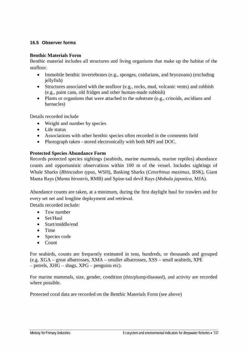
Ministry for Primary Industries Ecosystem and environmental indicators for deepwater fisheries • 137
16.5 Observer forms Benthic Materials Form Benthic material includes all structures and living organisms that make up the habitat of the seafloor.
• Immobile benthic invertebrates (e.g., sponges, cnidarians, and bryozoans) (excluding jellyfish)
• Structures associated with the seafloor (e.g., rocks, mud, volcanic vents) and rubbish (e.g., paint cans, old fridges and other human-made rubbish)
• Plants or organisms that were attached to the substrate (e.g., crinoids, ascidians and barnacles)
Details recorded include
• Weight and number by species • Life status • Associations with other benthic species often recorded in the comments field • Photograph taken - stored electronically with both MPI and DOC.
Protected Species Abundance Form Records protected species sightings (seabirds, marine mammals, marine reptiles) abundance counts and opportunistic observations within 100 m of the vessel. Includes sightings of Whale Sharks (Rhincodon typus, WSH), Basking Sharks (Cetorhinus maximus, BSK), Giant Manta Rays (Manta birostris, RMB) and Spine-tail devil Rays (Mobula japonica, MJA). Abundance counts are taken, at a minimum, during the first daylight haul for trawlers and for every set net and longline deployment and retrieval. Details recorded include:
• Tow number • Set/Haul • Start/middle/end • Time • Species code • Count
For seabirds, counts are frequently estimated in tens, hundreds, or thousands and grouped (e.g. XGA – great albatrosses, XMA – smaller albatrosses, XSS – small seabirds, XPE – petrels, XHG – shags, XPG – penguins etc). For marine mammals, size, gender, condition (thin/plump/diseased), and activity are recorded where possible. Protected coral data are recorded on the Benthic Materials Form (see above)

138 • Ecosystem and environmental indicators for deepwater fisheries Ministry for Primary Industries
Length frequency forms (MDBD and SMLF forms) Length frequencies are taken as required. Observers are briefed before each trip as to which species are to be measured and how often. Two types of form are used, depending on the number of fish available to measure: MDBD form (Middle Depths Biological Data) For 20 fish or less from a single tow/set. SMLF form (Stock monitoring Length Frequency) For 21 fish or more from a single tow/set. Samples are generally 100–150 fish. These forms record details of:
• Length • Sex • Gonad stage (females only) • Otoliths collected • Sample weight • Measurement method
Non-Fish Bycatch Form (seabird, marine mammals, protected fish and marine reptiles). Used whenever an interaction occurs between a seabird, marine mammal, protected fish or marine reptile and the fishing vessel. This form is used for captures and interactions only (not sightings). The working definition of an interaction is any animal which needs assistance to leave the vessels i.e., deck-strikes where the animal is stunned or injured. However if a bird lands on the vessel and then leaves it is not recorded as an interaction. Live animals captured are photographed where possible then released. This form records:
• Species code • Capture method • Life status • Injury status • Length • Sex • Samples taken (e.g., photograph, teeth, stomach, ovary, tissue sample) • Fate (e.g., released alive, discarded, retained as a specimen)
Catch Effort Logbook (CELB) Form Lists details of location, timing, operational details, catch, and discards for each individual trawl event. Shooting:
• Target species • Fishing gear used • Offal being discharged (y/n)
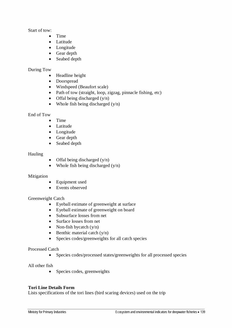
Ministry for Primary Industries Ecosystem and environmental indicators for deepwater fisheries • 139
Start of tow: • Time • Latitude • Longitude • Gear depth • Seabed depth
During Tow
• Headline height • Doorspread • Windspeed (Beaufort scale) • Path of tow (straight, loop, zigzag, pinnacle fishing, etc) • Offal being discharged (y/n) • Whole fish being discharged (y/n)
End of Tow
• Time • Latitude • Longitude • Gear depth • Seabed depth
Hauling
• Offal being discharged (y/n) • Whole fish being discharged (y/n)
Mitigation
• Equipment used • Events observed
Greenweight Catch
• Eyeball estimate of greenweight at surface • Eyeball estimate of greenweight on board • Subsurface losses from net • Surface losses from net • Non-fish bycatch (y/n) • Benthic material catch (y/n) • Species codes/greenweights for all catch species
Processed Catch
• Species codes/processed states/greenweights for all processed species All other fish
• Species codes, greenweights Tori Line Details Form Lists specifications of the tori lines (bird scaring devices) used on the trip
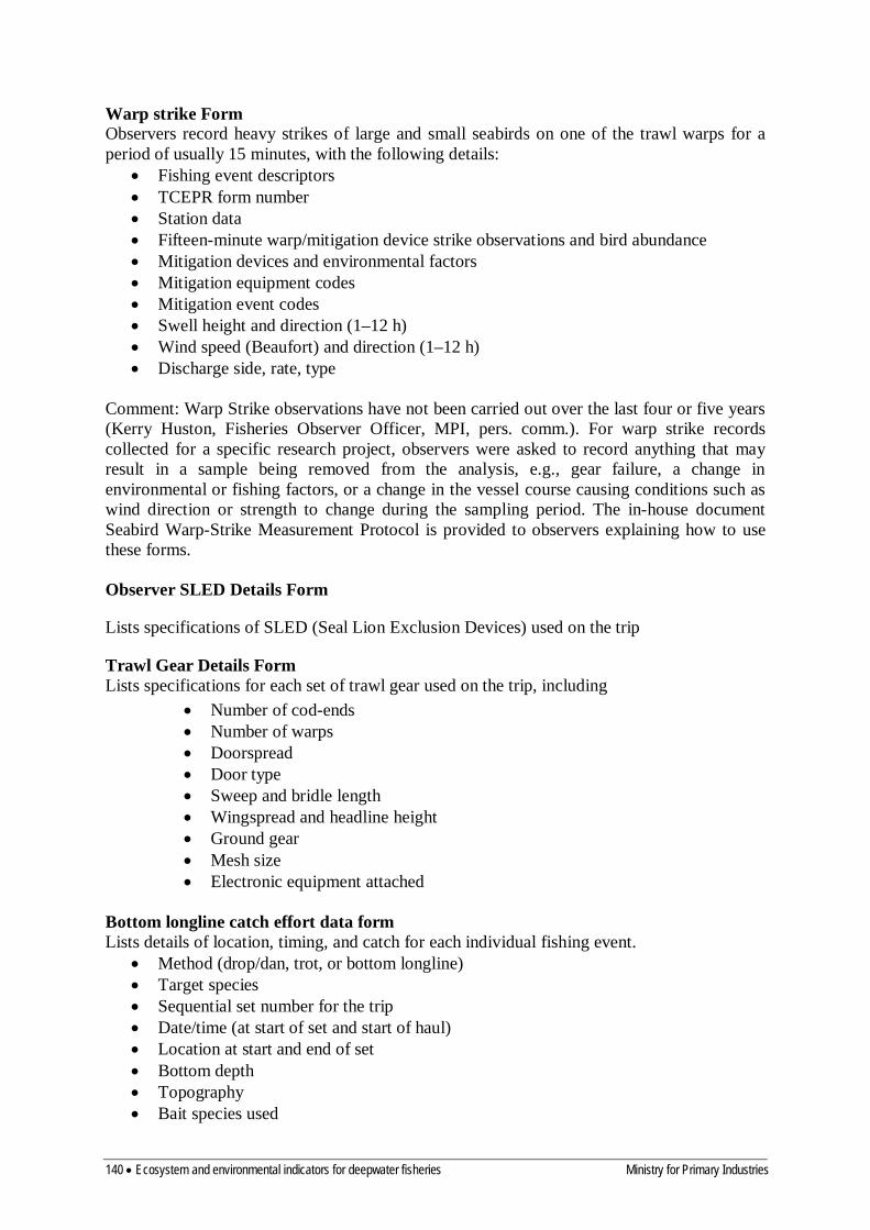
140 • Ecosystem and environmental indicators for deepwater fisheries Ministry for Primary Industries
Warp strike Form Observers record heavy strikes of large and small seabirds on one of the trawl warps for a period of usually 15 minutes, with the following details:
• Fishing event descriptors • TCEPR form number • Station data • Fifteen-minute warp/mitigation device strike observations and bird abundance • Mitigation devices and environmental factors • Mitigation equipment codes • Mitigation event codes • Swell height and direction (1–12 h) • Wind speed (Beaufort) and direction (1–12 h) • Discharge side, rate, type
Comment: Warp Strike observations have not been carried out over the last four or five years (Kerry Huston, Fisheries Observer Officer, MPI, pers. comm.). For warp strike records collected for a specific research project, observers were asked to record anything that may result in a sample being removed from the analysis, e.g., gear failure, a change in environmental or fishing factors, or a change in the vessel course causing conditions such as wind direction or strength to change during the sampling period. The in-house document Seabird Warp-Strike Measurement Protocol is provided to observers explaining how to use these forms. Observer SLED Details Form
Lists specifications of SLED (Seal Lion Exclusion Devices) used on the trip
Trawl Gear Details Form Lists specifications for each set of trawl gear used on the trip, including
• Number of cod-ends • Number of warps • Doorspread • Door type • Sweep and bridle length • Wingspread and headline height • Ground gear • Mesh size • Electronic equipment attached
Bottom longline catch effort data form Lists details of location, timing, and catch for each individual fishing event.
• Method (drop/dan, trot, or bottom longline) • Target species • Sequential set number for the trip • Date/time (at start of set and start of haul) • Location at start and end of set • Bottom depth • Topography • Bait species used

Ministry for Primary Industries Ecosystem and environmental indicators for deepwater fisheries • 141
• Percentage of hooks baited • Catch by species (weight and number of fish)
Setting Observations form (longline) Vessel, gear, and environmental details during setting of the longline
• Vessel speed and heading – for all course changes • Wind direction and force (Beaufort) – for all course changes • Air pressure, temperature, and visibility • Cloud cover • SST • Gear details including number of hooks, length of line and snoods, distance of hooks
off seabed, bait condition (frozen or thawed), and offal discharge (Y/N) • Details of tori pole usage • Seabird and marine mammal abundance counts
Hauling Observations form As for setting observations form but also;
• Evidence of fish damage by marine mammals • Seabirds and marine mammals captured (observed as well as not observed) • Deck Log – tallies of numbers of fish caught, landed, and discarded by species. Note:
the deck log details are not transferred to cod (or any other) database. Purse seine catch effort set details form
• Sequential set number • Method • Target species • Details of the school being targeted (location, association (boil-up, FAD, etc), how
was it spotted) • SST, sea state, sea depth • Total catch, and losses during retrieval • Seabird and marine mammal and turtle observations • Catch by species
Vessel activity log A running log of the vessels activities during a trip, for example:
• Searching for a school • Travelling to a school it has been notified of • Fishing • Sheltering due to bad weather • Steaming to port
Observer Setnet Gear form
• Net ID – individual code for each net used • Details of net configuration (height, mesh size, floats, ground weights etc) for each
net
Observer Setnet Catch/Effort Form

142 • Ecosystem and environmental indicators for deepwater fisheries Ministry for Primary Industries
• Sequential set number • Target species • Date, time, position at start and end of set • Bottom depth • Nets used (Net IDs) – where multiple nets joined using spacers • Net on bottom (Y/N/U) • Offal and whole fish discharge during setting and hauling (Y/N) • Non fish bycatch (Y/N) • Benthic materials (Y/N) • Catch and discards by species (greenweight)
16.6 Databases relevant to deepwater fisheries data collection Specimen Ageing (age) The age database contains a catalogue of ageing material and information on the age of mostly fish derived from this material, which is primarily otoliths, and in some instances scales, vertebrae, teeth, spines, and statoliths. The ageing material has been acquired from a variety of sources within New Zealand and covers over 50 species of fish. Centralised Observer Database (cod) The cod database contains data collected by Ministry for Primary Industries Observers on commercial fishing vessels. cod contains the catch and effort information for observed vessels, length frequency, biological and ageing materials data for commercial species as recorded by the observers, as well as relevant trip and tow information. Cod replaces the earlier observer databases obs, obs_lfs and l_line . Deepwater Catch (dw_cdb) The dw_cdb database contains partially groomed commercial catch and effort data from deepwater fisheries (orange roughy and oreo) used for stock assessments. Fish Catch Effort (fish_ce) The fish_ce database contains catch effort data from a variety of species that has been groomed as part of the stock assessment process. Longline Sampling (l_line) The l_line database contains comprehensive information collected by Scientific Observers placed on surface longline vessels (both foreign and domestic) in the New Zealand tuna fishery (comparable data from bottom longliners is stored in obs_lfs). Data includes information on gear types, catch and effort, and incidental seabird and marine mammal bycatch. This database was replaced by the cod database in 2009. Marlin Metadata (marlin) The marlin database houses the metadata about Ministry for Primary Industries databases and about data produced from fisheries research projects. Metadata provides information about the content, quality, condition, and other characteristics of data. Marlin includes information on datatypes, data volume, and database location. Fisheries Statistics Unit Catch Effort (new_fsu) The new_fsu database contains commercial catch-effort data collected and managed by the Fisheries Statistics Unit (FSU) prior to the establishment of the QMS. The FSU was disbanded in November 1988, therefore the 1988 and 1989 datasets are generally incomplete. Statistics back to 1972 were collected for some fisheries, which are included in this database.

Ministry for Primary Industries Ecosystem and environmental indicators for deepwater fisheries • 143
Fisheries statistics collected prior to 1983 are referred to as ‘pre-FSU’ in the database documentation. Non-fish bycatch (non-fish bycatch ) The non-fish bycatch database contains data on the incidental catch of protected species such as marine mammals and birds, reported by commercial fishers. Scientific Observer (obs) The obs database contains comprehensive catch effort data recorded by Scientific Observers placed on trawl vessels in New Zealand fisheries, including conversion factor data. This database was replaced by the cod database in 2008. Observer Length Frequency (obs_lfs) The obs_lfs database contains comprehensive biological (eg. length frequency, weight, gonad stage) and non-fish bycatch information collected by Scientific Observers from trawl and bottom longline vessels (additional to observer catch effort information). This database also incorporates observer-collected data from the squid fishery, which was housed in the squid database until 2001. This database was replaced by the cod database in 2008. Research Database (rdb) The rdb database contains all Ministry for Primary Industries reference codes that are used in the collection and checking of fisheries related data. Reference codes include, for example, species codes, area codes, method codes and biological codes. Regional Catch Effort (regional_ce) The regional_ce database contains catch and effort information from New Zealand fishing vessels operating outside the EEZ: for example, purse seine vessels in the South Pacific and longline vessels in CCAMLR waters. Arrow Squid Fishery Catch Effort (squ_ce) The squ_ce database contains a discrete time series (1989–1994) copy of commercial catch effort data (all methods) from the New Zealand arrow squid fishery. Vessel (vessel) The vessel database contains a groomed version of registration data for vessels that have fished in New Zealand waters.