Economics of Networks Difusion Part - MIT OpenCourseWare · Look at limits as. n. æŒ, large...

Economics�of�Networks� Difusion�Part�2

Evan�Sadler Massachusetts� Institute� of� Technology

Evan Sadler Difusion 1/34

!

!

!

Agenda

• Recap of last time, contagion and mean-field diffusion• The configuration model• Diffusion in random graphs• Monopoly pricing with word-of-mouth communication

Material not well-covered in one place. Some suggested reading: Jackson Chapter 7.2; “Word-of-Mouth Communication and Percolation in Social Networks,” A. Campbell; “Diffusion Games,” E. Sadler


Binary Coordination with Local Interactions

Recall our simple game:

0 1

0 (q, q) (0, 0)

1 (0, 0) (1 ≠ q, 1 ≠ q)

Two pure-strategy equilibria

Play simultaneously with many neighbors• Choose 1 if at least fraction q of neighbors choose 1• Myopic best response, can the action spread?

Cohesion can block contagion, but neighborhoods can’t grow toofast


! !

Mean-Field Difusion

An alternative framework• Distributional knowledge of the network structure• Adopt behavior iff expected payoff exceeds cost

Bayes-Nash equilibrium of static game equivalent to steady-stateof mean-field dynamics• Draw a new set of neighbors a every time step

Key phenomenon: tipping points

Relate steady state to network degree distribution


!

Random Graphs

Today, a third approach• Distributional knowledge of the network structure• Diffusion through a fixed graph

People get exposed to something new• Behavior, product, information...

Choose whether to adopt or pass it on

Stochastic outcomes, viral cascades


A Few Examples

Spread of new products through referral programs

Spread of rumors about Indian demonetization policy (Banerjeeet al., 2017)

Spread of news stories on social media• Maybe fake ones...

Spread of microfinance participation (Banerjee et al., 2013)


Questions

Basic:• How many people adopt?• How quickly does it spread?• Who ends up adopting?

Some implications:• Targeted seeding• Pricing strategies


First: The Configuration Model

Recall the configuration model from the first half of the course• This is how we will generate our networks

Start with n nodes, degree sequence d(n) = (d1, d2, ..., dn)• Degree is number of neighbors a node has

Take a uniform random draw of graphs with the given degreesequence

Look at limits as n æ Œ, large networks• Assume {d(n)} converges in distribution and expectation to D


The Configuration Model

Can think of D as a histogram• P(D = k) is the fraction of nodes with degree k

Questions about the configuration model:• What do the components look like?• Is there a “giant” component?• How big is it?• How far are typical nodes from each other?

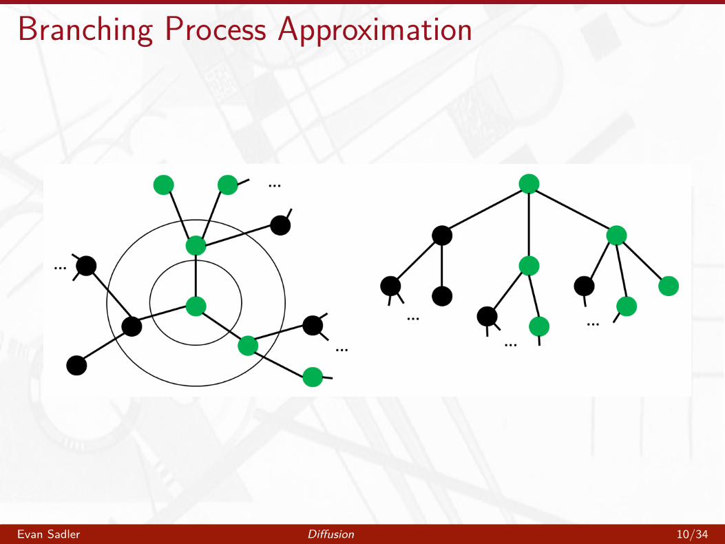
Key idea: branching process approximation


Branching Process Approximation


�

�

Branching Processes

Let Z œ c(N) be a probability distribution

Start from a single root note, realize offspring according to Z

Each node in the first generation realizes offspring independently according to Z

And so on...


!

!

Branching Processes: Extinction

What is the probability that the process goes extinct?

• Total number of offspring is finite

Key tool: the generating functionŒÿ

g(s) = P(Z = k)s kk=0

Well-defined for k œ [0, 1]Solve recursion: probability I go extinct is probability all my offspring go extinct

Œÿk

› = P(Z = k)› = g(›)k=0

Extinction probability is unique minimal solution to › = g(›)• Survival probability „ = 1 ≠ ›


�

�

�

Branching Processes: Growth Rate

Expected number of offsprt

ing E[Z] © µ• Generation t contains µ nodes in expectation

Write Zt for the random number of total offspring in generation t• The process Yt © Z

µtt is a martingale

By the martingale convergence theorem:• As t æ Œ, Yt converges almost surely• Implication: „ > 0 i µ > 1 (one exception: Z = 1 w.p.1)


�

�

Connecting to the Random Graph

Heuristically, breadth first search starting from a random nodelooks like a branching process• The “characteristic branching process” T for the graph

Root realizes offspring according to D

After the root, two corrections• Friendship paradox• Don’t double count the parent

Subsequent nodes realize offspring according to DÕ

= d) = P(D = d + 1) · (d + 1)P(DÕ

E[D]


The Law of Large Networks

Define flk = P(|T | = k), Nk(G) the number of nodes incomponents of size k, Li(G) the ith largest component

TheoremSuppose d(n) æ D in distribution and expectation, and G(n)

is

generated from the configuration model with degree sequence

d(n). For any ‘ > 0, we have

limnæŒ

P A----

Nk(G(n))n

≠ flk

---- > ‘B

= 0, ’ k

limnæŒ

P A----

L1(G(n))n

≠ flŒ

---- > ‘B

= 0

limnæŒ

PA

L2(G(n))n

> ‘

B

= 0.


The Law of Large Networks

For large graphs, network structure completely characterized bythe branching process• Distribution of component sizes• Size of giant component

Note: need DÕ non-singular

Proof is beyond our scope


Survival Probability of T

Fun fact: if g(s) is the generating function for D, then gÕ

µ (s) is

the generating function for DÕ:Œ

k=0Œ

k=1Œ

ÿ

k=0

ÿ

ÿ

d dÕ(s) = g(s) = P(D = k)s kg d ds s

kP(D = k)s k≠1=

(k + 1)P(D = k + 1)s k=

If › solves µ› = gÕ(›), survival probability of T is „ = 1 ≠ g(›)

• Giant component covers fraction „ of the network


Typical Distances

Define ‹ = E[DÕ], H(G) distance between two random nodes inthe largest component of G

TheoremA giant component exists if and only if ‹ > 1. In this case, for

any ‘ > 0 we have

limnæŒ

P A----

H(G) log‹ n

≠ 1---- > ‘

B

= 0

Typical distance between nodes is log n‹

• Relates to growth rate of the branching process T


A Difusion Process

People learn about a product through word-of-mouth• i.i.d private values v distributed uniformly on [0, 1]• Price p

If I learn about the product, buy if v > p

• If I buy, my friends hear about it, make their own choices

Suppose n individuals are linked in a configuration model, andone random person starts out with the product• How many people end up buying?• How long does it take to spread?


�

Outcome Variables

Let Xn(t) denote the (random) number of purchasers after tperiods in the n person network

Define extent of adoption

Xn(t)– n = lim

tæŒ n

For x œ (0, 1), diffusion times I

Xn(t) J

· n(x) = min t : (Œ) Ø xXn

Will characterize – n and · n for large n


Percolation in the Configuration Model

If I buy, each neighbor will buy with independent probability1 ≠ p• Adoption spreads through a subgraph• As if we delete each person with independent probability p

The percolated graph is also a configuration model, degreedistribution Dp

• Realize degree according to D, delete each link withprobability p

• Binomial distribution with D trials and success probability1 ≠ p

Generating function for Dp:

gp(s) = g (p + (1 ≠ p)s)


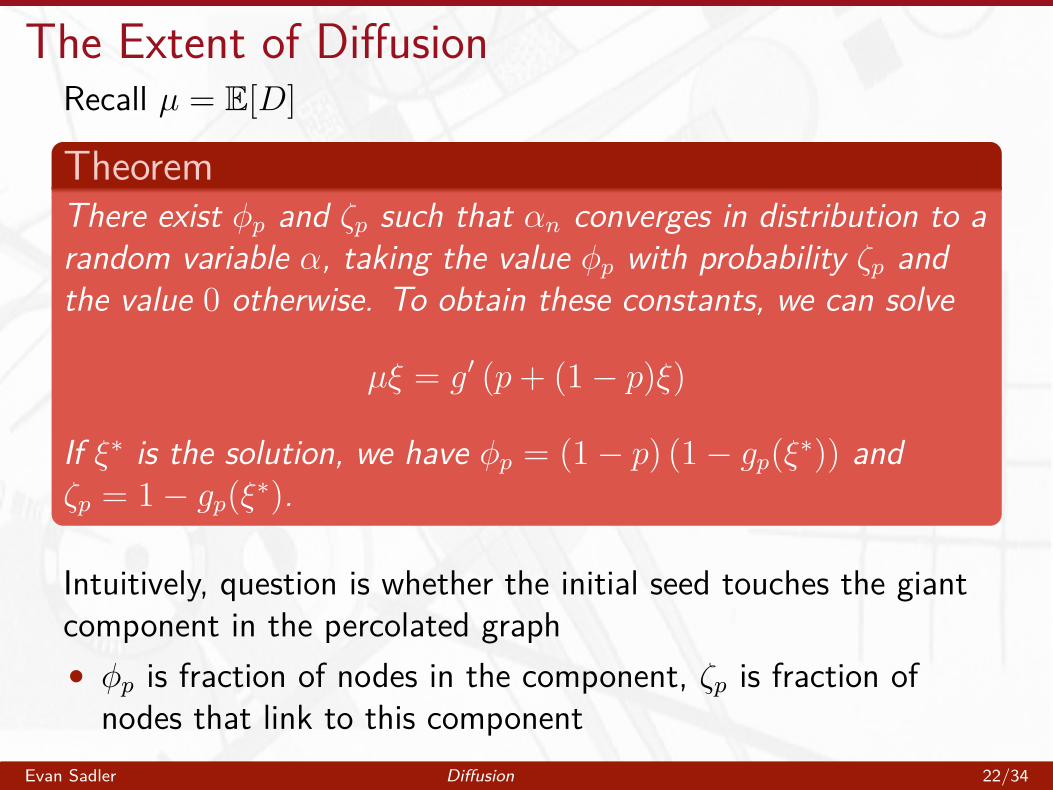
Theorem

The Extent of Difusion

Recall µ = E[D]

• „p is fraction of nodes in the component, ’ p is fraction ofnodes that link to this component


There exist „p and ’ p such that – n converges in distribution to a random variable –, taking the value „p with probability ’ p and the value 0 otherwise. To obtain these constants, we can solve

µ› = g Õ (p + (1 ≠ p)›)

If ›ú is the solut

ion, we have „p = (1 ≠ p) (1 ≠ gp(›ú)) and

’ p = 1 ≠ gp(›ú).

Intuitively, question is whether the initial seed touches the giant component in the percolated graph

The Extent of Difusion

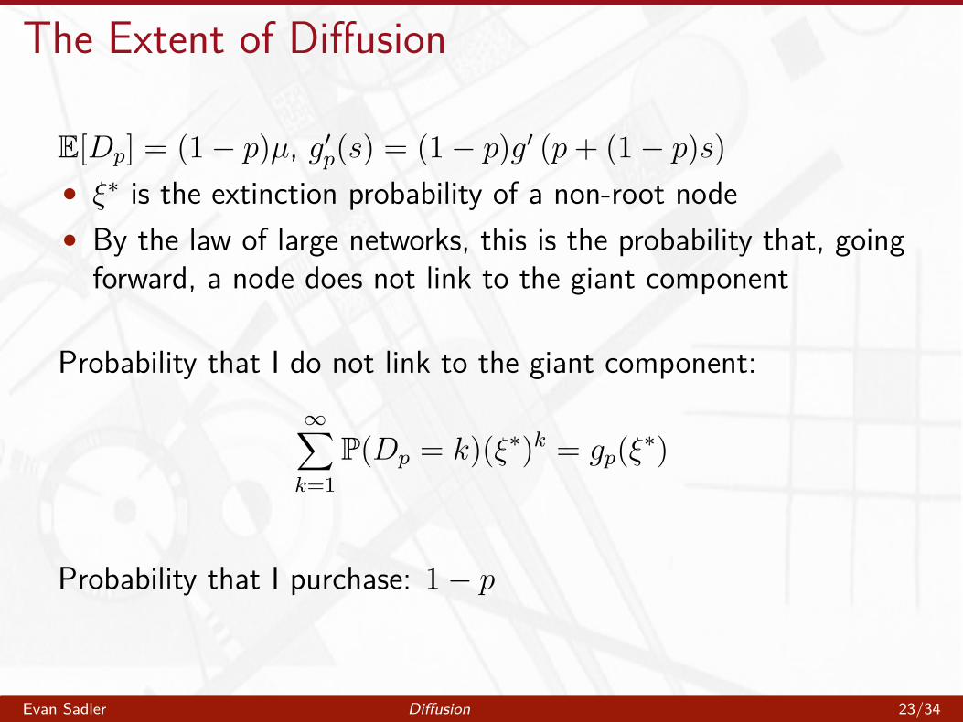
E[Dp] = (1 ≠ p)µ, gpÕ (s) = (1 ≠ p)gÕ (p + (1 ≠ p)s)

• ›ú is the extinction probability of a non-root node

• By the law of large networks, this is the probability that, goingforward, a node does not link to the giant component

Probability that I do not link to the giant component:Œÿ

kP(Dp = k)(› ú) = gp(› ú)k=1

Probability that I purchase: 1 ≠ p


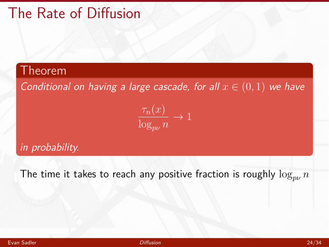
The Rate of Difusion

TheoremConditional on having a large cascade, for all x œ (0, 1) we have

· n(x) logp‹ n

æ 1

in probability.

The time it takes to reach any positive fraction is roughly logp‹ n


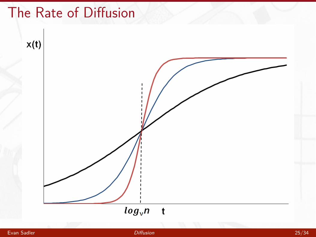
The Rate of Difusion


Comparative Statics

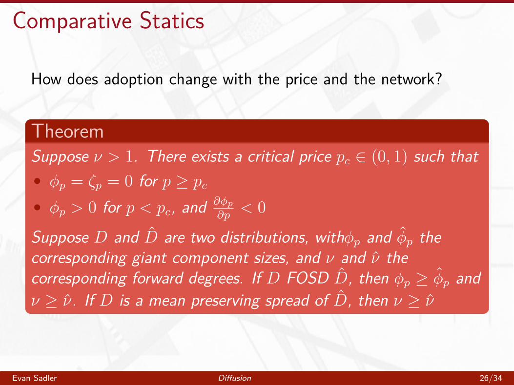
How does adoption change with the price and the network?

TheoremSuppose ‹ > 1. There exists a critical price pc œ (0, 1) such that

• „p = ’ p = 0 for p Ø pc

• „p > 0 for p < pc, and ˆ„p

ˆp < 0Suppose D and D̂ are two distributions, with„p and „̂p the

corresponding giant component sizes, and ‹ and ‹̂ the

corresponding forward degrees. If D FOSD D̂, then „p Ø „̂p and

‹ Ø ‹̂. If D is a mean preserving spread of D̂, then ‹ Ø ‹̂


�

�

�

Comparative Statics

For suffciently high prices, there is no adoption, impossible toget viral cascade

Below the critical price, adoption is decreasing in price• At pc, derivative makes a discontinuous jump

Making the network more dense leads to more adoption and faster diffusion• Mean preserving spread makes diffusion faster, but may not

lead to more adoption


Example

Suppose D takes the value 3 for sure, D̂ takes values 1 or 5 withequal probability

Under D, extinction probability solves

› = (p + (1 ≠ p)›)2 =∆ › = min 1,[

Y]

¥ 1

A B2Z^p

1 ≠ p \

For p close to zero, › is close to zero, „p

Under D̂, extinction probability solves

6› = 1 + 5 (p + (1 ≠ p)›)4

For p close to zero, › close to 0.17, „p ¥ 0.83


A Pricing Problem

Suppose a monopolist is selling this product and wants to choosep to maximize profits• Constant marginal cost c < 1

Assume a fraction ‘ ¥ 0 of the population gets seeded at random• For large networks, guaranteed to hit the giant component

Total demand is fraction Q(p) = „p = (1 ≠ p) (1 ≠ gp(›ú)) of thepopulation

Choose p to maximize Q(p)(p ≠ c)


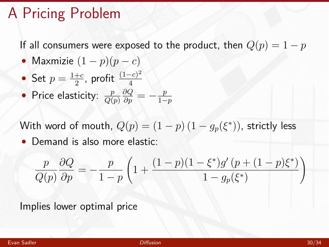
A Pricing Problem

If all consumers were exposed to the product, then Q(p) = 1 ≠ p• Maxmizie (1 ≠ p)(p ≠ c)

1+c• Set p = 2 , profit (1≠4 c)2

p ˆQ p• Price elasticity: = ≠Q(p) ˆp 1≠p

With word of mouth, Q(p) = (1 ≠ p) (1 ≠ gp(›ú)), strictly less• Demand is also more elastic:

p ˆQ p A

(1 ≠ p)(1 ≠ ›ú)gÕ (p + (1 ≠ p)›ú)B

= ≠ 1 + Q(p) ˆp 1 ≠ p 1 ≠ gp(›ú)

Implies lower optimal price


Price Comparative Statics

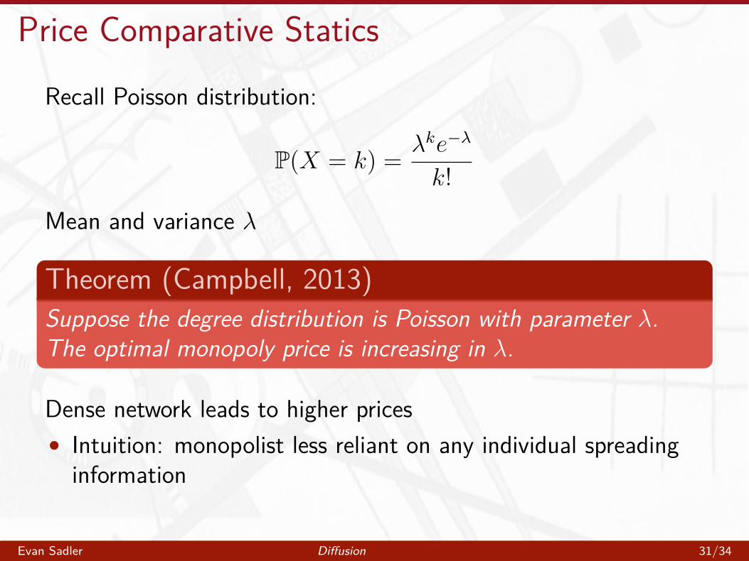
Recall Poisson distribution:

eP(X = k) = ⁄k

k!≠⁄

Mean and variance ⁄

Theorem (Campbell, 2013)Suppose the degree distribution is Poisson with parameter ⁄.

The optimal monopoly price is increasing in ⁄.

Dense network leads to higher prices• Intuition: monopolist less reliant on any individual spreading

information


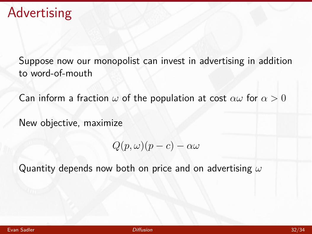
Advertising

Suppose now our monopolist can invest in advertising in additionto word-of-mouth

Can inform a fraction Ê of the population at cost –Ê for – > 0

New objective, maximize

Q(p, Ê)(p ≠ c) ≠ –Ê

Quantity depends now both on price and on advertising Ê


Advertising

Word-of-mouth complements advertising• Customers exposed through advertising will inform additional

people

Hard to jointly solve for optimal p and Ê, but...

TheoremSuppose the degree distribution is Poisson with parameter ⁄.

Price and advertising are strategic complements.

All else equal, higher prices tend to go with more advertising


�

� �

Takeaways

Discrete network diffusion models help us think about viral cascades• Component sizes in percolation network

Faster diffusion ”= more diffusion

Word-of-mouth leads to more elastic demand, tends to lower prices

Next time: models of network formation


MIT OpenCourseWare https://ocw.mit.edu

14.15J/6.207J Networks Spring 2018

For information about citing these materials or our Terms of Use, visit: https://ocw.mit.edu/terms.

Economics of Networks Difusion Part - MIT OpenCourseWare · Look at limits as. n. æŒ, large...

Documents

Transcript of Economics of Networks Difusion Part - MIT OpenCourseWare · Look at limits as. n. æŒ, large...