Economics of Earnings: Human Capital Approach

Sources: Becker, Human Capital Ch. 2 (introductory), Acemoglu's Ch. 1 (p. 5-11)Polachek and Siebert, Ch. 2-4 (basic models)

Lemieux (2006) “The Mincer Equation” (empirical issues)Berndt, Ch. 5 (empirical issues)

Human Capital Approach

- Productivity of a worker is linked to attributes of the worker- acquired skills - innate ability and pre-labour market influences.

- Human capital models are concerned with acquired skills.- could extend to think of parental investment in child’s skills

(some of pre-labour market skills may also reflect investmentby parents)

- Extra human capital boosts productivity (value of output per unit of L) by:- makes it possible to do a given task better;- makes it possible to do higher value tasks; - makes a worker more adaptable / flexible (T. Schulz);- makes workers better suited to a structured environment (Bowles and Gintis).

- Comparability to physical capital- affects productivity - result of an investment decision.

- Measures of human capital (HC):- education: - quantity: years of schooling, degrees and other qualifications.

- quality: of instruction, resources per student, etc.

- on-the-job training: likely linked to work experience.

- General vs. specific HC: general is of value to many employers; specific HC of value to one employer (general HC is our main concern).

- We will concentrate on the earnings equation literature. - aims to explain the shape of earnings profiles;- aims to explain differences between profiles by education.

- Note productivity-wages link from labour demand theory (must be general HC to work):

↑Skills → ↑Productivity → Employer competition → ↑Wages

- Investment theory suggests a supply reason for an acquired-skill wage link.- need to pay a skill premium if people are to have an incentive to acquire skills.

1

Theoretical Models of Investment in Human Capital

Ben Porath Model

- See: Polachek and Siebert Ch. 2 and start of Ch.3.

- A model of investment in human capital and earnings determination.

- Potential Earnings (E) are a function of stock of human capital:

Et = w Kt

w = wage per unit of human capital (treat as fixed)K = stock of human capital

- “potential”: if no time is spent acquiring more human capital.

- Growth in potential earnings:

Et/t = w Kt/t

i.e., changes with changes in human capital.

- New human capital generated: Qt

- with no skill depreciation:

Qt = Kt/t

- assume new human capital is produced as follows:

Qt = (stKt)b

where:

s = share of existing human capital used to produce more HC (0≤s≤1)

0<b<1 = measure of productivity in producing HC (“ability”)

- Cost of human capital (foregone earnings):

Ct = w stKt i.e. assume K used to produce HC generates no income.

= w Qt1/b

2

marginal cost of human capital (MC):

Ct/Qt = w Qt(1-b)/b/b until s=1

= at s =1 (can’t produce any more)

(shape of upward sloping portion? linear if b=.5 , flatter at higher Q if b between .5 and 1, steeper at higher Q (as in picture if 0<b<.5)

- Rise in w shifts MC up ; rise in ‘b’ shifts MC down.

3

- Marginal Benefit of extra HC (MB):

- Each extra unit of HC generates: w in each future period.

- Assume retires at age 65

- Present value of an extra unit of HC created in period t:

w + … + w (1+i) (1+i)65-t

= (w/i) [ 1 - 1/(1+i)65-t ]

- this is the marginal benefit of human capital.

4

- Optimal HC investment choice:

- keep investing as long as marginal benefit > marginal cost

- optimal when: marginal cost = marginal benefit

w Qt(1-b)/b/b = (w/i) [ 1 - 1/(1+i)65-t ]

so:

Qt = { (b/i) [ 1 - 1/(1+i)65-t ] }b/(1-b) (this is Qbest in diagram)

- more HC creation (higher Q):

- higher is b (shifts MC down)- lower is i (shifts MB up)- lower is t (shifts MB up ; Qmax also smaller)

- condition above is only true for an interior solution.

5

- Corner solution?

s=1 : all time used for HC creation (“schooling”)

when most likely? - young (low t, low K)- low i - high b

- Actual earnings (Y) profile:

Yt = Et - w stKt

= w(1-st)Kt

- actual earnings profile over time?

- actual earnings 0 if s=1 when young- K rises with t- s falls with t- actual earnings rise with t.

- rises more quickly than potential earnings.- rises at a diminishing rate (Y approaches E as s falls toward 0 as

the person ages)- this is roughly the shape of typical earnings profiles.

6

- Costs of Producing Human Capital:

- Ben Porath model: costs are all foregone earnings

- Missing are: direct costse.g. tuition, books, etc.

likely less than foregone earnings but they pose issues.

- Family Background, Ability and Human Capital Acquisition:

- Financing human capital acquisition:

- loans against human capital: - private sector reluctant. - high interest rate to compensate for risk or

borrowing constraints.

- family as an alternate source of finance.

- could introduce family wealth via level of i.

- rich families: lower i, more HC.- poor families: higher i, less HC.

7

- Ability to Produce Human Capital (b):

- May be innate (nature)

- May be developed in the home to some degree (nurture)

- Elementary and secondary school quality may affect this.

- Return to a unit of human capital (w):

- family influences? - information, contacts, connections.

Human capital choices of men and women:

- Ben Porath model assumes that people plan work all periods in which s<1 (until retirement).

- Women:- more intermittent patterns of participation, i.e., having and

raising children

- Human capital acquisition and this?- fewer working periods- other things equal K is worth less.- less human capital investment.

- occupational choice and this.- women choose jobs requiring less HC.- women choose jobs in which HC is less likely to depreciate while

out of the labour force.

- see Polachek and Siebert pp. 155-158.

- a good prediction until early 1980s or so? - 2014: women are now more likely to invest in some types of HC

(post-secondary education) - interpreting this via the model?

- Less intermittency due to family?- Earnings premia for HC: higher (especially for women? –

then w higher for women in the model)

8

Mincer’s Human Capital Earnings Functions

- Basic source: J. Mincer (1974) Schooling, Experience and Earnings

- Follow: Polachek and Siebert’s presentation Ch. 4.

- Some observations:- Illustration of earnings-experience profiles by education group. - Positive effect of education on earnings. - Positive but diminishing effect of experience on earnings.

- Notation: r = average annual rate of return on human capital investment. e.g. r=.05 (5%) S = total number of years of full-time schoolingCt = human capital investment in time t.Et = potential earnings at time t.Yt = actual earnings at time t = Et - Ct

st = Ct/Et measures investment in human capital in time t (share of earning capacity that goes to creating new human capital).

Potential earnings (E) in period 1:

E1 = E0 + r C0

= E0 + r s0E0

= E0 (1+ r s0)

Then in period 2: E2 = E0 (1+ r s0) + r C1

= E0 (1+ r s0) + r s1E1

= E0 (1+ r s0) (1+ r s1)

And in period t:

Et = E0 (1+ r s0) (1+ r s1) (1+ r s2)… (1+ r st-1)

In logs:

ln (E t )= ln ( E0 )+∑

i=0

t−1

ln (1+rsi )

Then since ln(1+rsi) rsi :

9

ln (E t )≃ ln( E0 )+r∑

i=0

t−1

si

- Now if during full-time schooling si=1 and this happens for the first “S” years:

ln (E t )≃ln ( E0 )+rS+r ∑

i=S+1

t−1

si

or more generally if returns to schooling (rs) differ from returns to other human capital investment (rp):

ln (E t )≃ ln ( E0 )+r s S+r p ∑

i=S+1

t−1

si

- It is likely that si will decline with age for example:

si = a –bi (s falls linearly with i)

- Then:

ln (E t )≃ ln ( E0 )+r s S+r p ∑

i=S+1

t−1

(a−bi )

- Call ET earnings of someone T years after schooling is completed (with T years of experience):

ln (ET )≃ln ( E0 )+r s S+r p ∑

i=0

T−1

(a−bi )

(note the sum is now defined to run over experience, i.e. i=0 is same as i=S+1 above)

ln (ET )≃ln ( E0)+r s S+r p aT−r p b(T−1)T /2

- This gives:

ln (ET )≃ln ( E0 )+r s S+a1T−a2T 2

where:a1 = rp(a+ b/2) a2 = rpb/2

10

- In terms of actual (Y) rather than potential earnings (E):

YT = ET (1-sT)

ln(YT)= ln(ET) + ln(1-sT) ln(ET) - sT

where: sT=a-bT

- Using this gives the most common human capital earnings function:

ln (Y T )≃ ln( E0)−a+r s S+(a1+b )T−a2T 2

Implied earnings-experience profiles:

- Quadratic profile. - diminishing effect of experience on earnings.

∂ ln(Y T )∂ T

=a1+b−2a2 T

- for high T could be negative (skills depreciation? done more formally in Polachek and Siebert's Ch4 appendix)

- Higher education, higher profile.

11

Earnings Functions: Implementation and Econometric Issues

- Some sources: T. Lemieux (2006) “The Mincer Equation Thirty Years after Schooling,

Experience and Earnings” From: Jacob Mincer, A Pioneer of Modern Labor Economics, Springer Verlag.

Berndt Ch. 5

(1) Possible Problems with the Dependent variable:

- What should the wage measure?

- usual variable is wage rate measure.

- ideal: all compensation (including all benefits)

- Wage Measure is often derived:

Hourly wage = (weekly wage)/(hours per week)

- measurement error may be significant in some jobs.e.g., irregular hours worked

- Limits:- Surveys sometimes place upper bounds on wage variables.

e.g., $50 and over.

- Minimum wage laws may put a floor on observed wage rates.

- Using OLS can result in biased earnings equation estimates if there are significant numbers of observations at the limits.

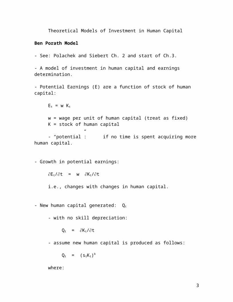
- Solution? - Estimate using “tobit” (see labour supply).

- Should the earnings measure be in logs?

- theoretical model suggests this is plausible but does it fit the data?

- Lemieux (2006):- notes attempts to test log-linearity of the relationship.

- Box-Cox method: nests log-log, log-linear and linear models (test value of 1 key parameter)

12

Heckman and Polachek (1974) used this and could not reject the log-linear model.

- Fortin and Lemieux (1998): - used a rank regression model: a more general approach.

- “assumption of log-linearity is very accurate for most of the range of the distribution”.

- where do problems arise? Near minimum wages – they may have compressed wages at the low end of the wage distribution.

(2) Measuring experience:

- All work experience? Full-time jobs? Current job only?

- Most surveys do not ask an experience question.

- Possible proxies?

- Age: - will obviously overstate experience. - earnings profiles steeper for more educated (higher “r”)

when this is used.

- Potential experience: (Age – Years in School – 5)- Mincer proposed this type of measure.- Eliminated differences in profile slopes (see diagram from

Lemieux). - not too bad for men, but women?

- Predicting experience:- estimate a relationship on a dataset with experience.- use this to predict experience on the dataset without

experience.

(3) Measuring educational attainment:

- Mincer’s function: years of schooling the key variable.

- Is it the best measure of attainment?- vs. qualifications obtained

- Often datasets contain “highest level of educational attainment”

13

e.g., University degree, High school graduate.

- set of educational attainment dummies used in place of “years of schooling”

- interpreting the coefficients?

ln W = a + b HS + c UNI + …

HS = 1 if high-school education, 0 otherwise.UNI=1 if university degree, 0 other wise.Default group: less than high-school.

b = premium (in log-wages) paid to HS=1 vs. less than high-school.

eb = Whs/Wnhs

so:eb –1 = proportion by which HS=1 wage exceeds No high school

wage.

(4) Functional form: Linear in Years of Education?

- Lemieux (2006) notes that different versions of theoretical human capital models can give concave or convex relationships between log-earnings and years of education.

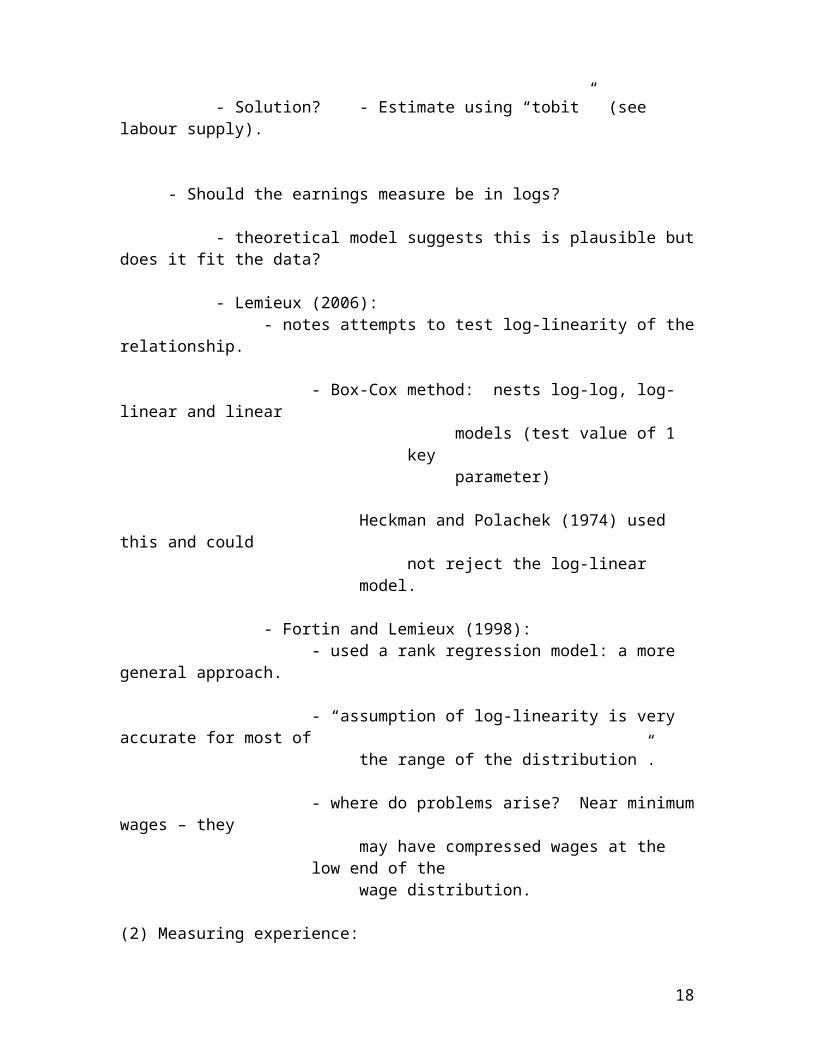
- “Credential” or “Sheepskin” effect arguments suggest that log-earnings jump upward after at the point where a credential is obtain rather than linearly with years of education.

e.g. jumps when you graduate from high school or university.

- Testing this? - convert “years of education” into a series of dummy variables (one for each year

of schooling).

- are the estimated coefficients consistent with linearity in education?

- See: Lemieux’s Figures 11.3-11.5

- US data for men: 1979-1981 sample: nearly linear in education but with a jump at

15-16 years of education.

14

Later years: relationship has become increasingly more convex, i.e. steepest at high years of education.

- notes estimating log-earnings with “years of schooling squared” as a regressor. Coefficient is significant in later years.

- So linearity inappropriate in recent years.

(5) Functional form: Quadratic experience?

- Is the quadratic form too restrictive?

- Lemieux’s Figures 11.6 to 11.8 suggest it is:

- Quadratic: - log-earnings rise too slowly for the first 10-15 years of experience;- log-earnings decline too much after 25 years of experience (should be

closer to stability).

- Higher order polynomial in experience is more accuarate: quartic polynomial.

(6) Functional form: Separability of Education and Experience Effects

- The Mincer equation suggests that extra education just produces a parallel shift in the log-earnings vs. experience relationship.

- Lemieux: - this worked well in earlier data.

- more recent data? University vs. high-school gap tends to decline with experience.

(does this reflect “cohort effects”?)

15

(7) Cohort effects:

- Theoretical model: - predicts log-earnings profile for a given individual: follows them over their

lifetime.

- other individuals starting at the same period might be expected to have similar profiles (assuming proper controls for differences between individuals).

- so age cohorts (same birth years may have similar profiles)

- but cohort-specific effects may give different profiles for different cohorts.

- Empirical implementation:

- Often uses cross-sectional microdata: so one point in time.

- Implicitly assumes that performance of older groups now is a good predictor of future outcomes of current younger groups.

e.g. what current 35 year olds are doing now is a good guess of what current 25 year olds will be doing in 10 years.

- There is evidence of substantial difference by cohort. e.g. Beaudry and Green (2000) Canadian Journal of Economics.

- This may account for some of the more recent problems with the Mincer equation: solution is to allow for cohort effect or to estimate cohort

specific profiles.

(could note cohort effects identification is difficult: age, time and cohort effects are linear combinations of one another)

(8) Omitted Variable Problems: Ability

- Ability is likely to positively affect earnings.

- Few datasets contain measures of ability.

- Error term captures effects of unobservable characteristics, including ability.

- Omitted regressors result in bias if they are correlated with other regressors.

- intuitively:coefficient on the included regressor will capture a mix of

16

it’s own true effect and the effect of the omitted regressor.

- Omitted ability and returns to education.- educational attainment: likely positively correlated with ability.

- estimated coefficients on education will capture:- effect of education on earnings- effect of ability on earnings.

- overestimate of the true effect of education.

- Approaches:

(a) Estimate returns to education by comparing observations with same ability but different educational levels.

- How (given ability not measured)?

- studies of twins: likely same natural ability – so differences in education between twins is more likely a pure skill effect.

- use of longitudinal (panel) data:

Say wages for person i at time t and time t+1 are:

lnWi,t = b0 + b1 IQi,t + b2 Si,t + b3 Xi,t + ei,t

lnWi,t+1 = b0 + b1 IQi,t+1 + b2 Si,t+1 + b3 Xi,t+1 + ei,t+1

IQ = ability, S = years schooling, X = experience.

- If b1 is stable and IQ does not change over time it is an example of a “fixed effect”.

- differencing then eliminates ability from the equation.

- so (given stable b’s):

lnWi,t = b2 Si,t + b3 Xi,t + ei,t

- estimation of this avoids the omitted ability problem.

- estimates effect of schooling by looking at effects of changes in S on lnW for the same person.

17

- a possible solution to the problem of “unobserved heterogeneity” in many other contexts.

(b) Studies with actual ability measures (e.g. test results).- only a few data sets have such data.

- unclear that bias is so severe a problem.

- but how good are these ability measures? (likely imperfect)

(c) Instrumental variables methods.- replace the education variable with an “instrument” for

educational outcomes (or changes to them) that is not correlated with ability.

- instrument must be correlated with education but not correlated with ability.

- Card (2001) “Estimating the Return to Schooling” Econometrica 1127-1160.

- Surveys the literature using instruments for education.

- Example instruments in this literature:

- Birthdate:- compulsory schooling laws: specify earliest age you can leave

school. - those whose birthdates mean they reach the compulsory age first

may have slightly less schooling.

- birthdate correlated with years schooling but not ability, family background or other key unobservables.

- Proximity to nearest college/university- positively correlated with educational attainment.- unlikely to be correlated with unobservables.

- Birth-cohort:- Use exogenous differences in cohort educational outcomes.- Exogenous sources of cohort differences?

- inter-cohort differences in school leaving laws.

18

- war and European educational outcomes- Lemieux and Card (2001): WWII veterans benefits (age

19-22 in 1946 and English speaking Canadian)

- Results of these studies?

- Estimated effect of education on earnings larger when IV methods are used.

- A puzzle? - ability story suggests they will be smaller!

- why? Unresolved (Card offers some possibilities).

(9) Sample selection Bias

- The sample of wage earners is not selected randomly.

e.g., participation decision: wage vs. reservation wage

self-employment vs. paid work: wage in paid employment matters.

- Result?- wage equation error term likely correlated with regressors.

- bias.

- Solution: Heckman’s two step procedure.

- estimate sample selection rule using probit.

- obtain estimate of inverse Mill’s ratio from the probit model.

- include this estimate as a regressor in the wage equation.

(10) Endogeneity problems

- Are explanatory variables endogenous and correlated with the error term.

e.g., experience: - reflects past labour force participation decisions- these reflect past wages- these reflect past wage equation error terms and

unobservable factors they may reflect.

19

- likely correlated with current error term.

- Similar arguments could be made for education e.g. education and ability.

Application: Estimating the Rate of Return to Education

- Earnings equations measure only measure the effects of human capital on earnings.

- Studies above ignore the direct costs of human capital investment.

- Framework for calculating rates of return on human capital.

- Let: ED0 be current level of educationED1 level with additional education.

Wt(EDi) = wage profile with education level EDi.DC = direct costs of educationG = graduation (G years from year 0)R = retirement (R years from year 0).i = discount rate

- In Period 0, Undertake additional education if:

∑t=G

R W t ( ED1)−W t ( ED0 )

(1+i )t > ∑t=0

G W t ( ED 0)

(1+i )t + ∑t=0

G DC t

(1+i )t

Present value of extra > Present value of + Present value ofwages foregone wages direct costs

- Determinants of the decision of Person at period 0:- Projected Wage profiles - discount rate:

- level of interest rate.- family resources.

- G- R-G (length of potential working life after graduation)- Ability:

- via G?

20

- DC: - scholarships- non-monetary costs: effort.

- Tuition and other direct costs.

- For the entire population: are enrolments rising or falling? Determinants:

- Projected Wage profiles- Distribution of personal discount rates

- distribution of family wealth.- Age distribution of population (R).- Distribution of ability.- Current tuition levels.

- Stock of people with ED1 right now:- Reflects past investment decisions.

- reflects past values of variables affecting the choice.- one set for each age cohort.

- Age distribution of population:- shares that faced each set of past conditions.

- Constraints?

- Ignored in this framework.

- Admissions standards, limited number of places can mean some who choose extra education do not get it.

- HC models tend to be models of "demand for HC" or "demand for education": implicitly assume supply is readily available.

- Internal rate of return (r) :

- value of the discount rate at which PV of Benefits equals PV of Costs of extra education.

- measures average annual rate of return on the investment.

- Calculating it:

∑t=G

R W t ( ED1)−W t ( ED0 )

(1+r )t = ∑t=0

G W t ( ED0 )

(1+r )t + ∑t=0

G DCt

(1+r )t

21

- obtain data, predictions of DC, W, G and R then solve for r.

- Private returns. vs. social returns.

- Private: private costs and benefits

e.g., - use after-tax wages- direct costs: tuition, extra living expenses.

- Public: social costs and benefits

- use pre-tax wage.- direct cost:

- include all costs of offering the degree not just tuition costs.

- Examples: go through an example study

- Boothby and Drewes (2006) "Post-secondary education in Canada: returns to university, college and trades education" Canadian Public Policy.

- See also results in Moussaly-Sergieh and Vaillancourt (2009) Extra Earnings Power: Financial Returns to University Education in Canada.

C.D. Howe Institute E-brief.

22