Working Paper Series Investment and Interest Rate Policy in the Open Economy

Stephen McKnight University of Reading, UK

Economics Analysis Research Group

EARG Working Paper No. 2007-011

stephen.mcknight@reading.ac.uk www.reading.ac.uk/earg

Investment and Interest Rate Policy in the Open

Economy

Stephen McKnight∗

University of Reading

October 2007†

Abstract

This paper presents a two-country sticky-price model that allows for capital and

investment spending. It analyzes the conditions for equilibrium determinacy un-

der alternative interest-rate rules that react to either domestic or consumer price

inflation. It is shown that in the presence of investment, real indeterminacy is con-

siderably easier to obtain once trade openness is permitted. Consequently we argue

that sufficiently open economies should adopt a backward-looking rule and suffi-

ciently closed economies should employ a current-looking rule, in order to minimize

policy induced aggregate instability.

JEL Classification Number: E32; E43; E53; E58; F41

Keywords: Real indeterminacy; Open economy macroeconomics; Interest rate rules;

Monetary Policy.

∗Correspondence address: Stephen McKnight, Department of Economics, University of Reading,Whiteknights, PO Box 219, Reading, RG6 6AW, UK. E-mail: Stephen.McKnight@reading.ac.uk.

†I would like to thank Roy Bailey, Ken Burdett, Joao Miguel Ejarque, Aditya Goenka, Mark Guzman,Kerry Patterson and Helmut Rainer. Financial assistance was gratefully provided by the Economic andSocial Research Council (ESRC). As always, the usual disclaimer applies.

1

1 Introduction

There is a large body of research that has considered the real indeterminacy implications

of designing interest-rate rules in sticky-price monetary models.1 The general conclusion

that emerges from the literature is that in order to rule out real indeterminacy the mon-

etary authority should follow the Taylor principle (i.e. an active policy stance), that is,

a policy that aggressively targets either expected inflation (e.g. Bernanke and Wood-

ford (1997), Clarida et al. (2000)) or current inflation (e.g. Kerr and King (1996)) by

raising the nominal interest rate by proportionally more than the increase in inflation.

However a number of recent studies have challenged the appropriateness of the Taylor

principle in preventing multiplicity of equilibrium once the economic environment allows

for capital and investment spending. Dupor (2001) introduces investment spending using

a continuous- time framework and shows that a passive policy stance is required for equi-

librium determinacy. In a discrete-time framework, Carlstrom and Fuerst (2005) show

that with the addition of capital and investment spending equilibrium “determinacy is

essentially impossible” under a forward-looking interest-rate rule.2 For current-looking

interest-rate rules, Carlstom and Fuerst (2005), Sveen and Weinke (2005) and Benhabib

and Eusepi (2005) all find that the Taylor principle is not a sufficient condition for deter-

minacy, although the range of indeterminacy generated is typically small.3

The purpose of this paper is to investigate the importance of investment spending

for equilibrium determinacy for economies that are open to international trade in goods

and assets. Using a discrete-time, money-in-the-utility function framework, this paper

develops a two-country, sticky-price model that allows for capital and investment spend-

ing.4 The conditions for real equilibrium determinacy are analyzed for forward, current

and backward-looking versions of the interest rate rule. In addition, two alternative price

1By real indeterminacy we simply mean that there exists a continuum of equilibrium paths, starting fromthe same initial conditions, which converge to the steady state.

2Interestingly, Kurozumi and Van Zandweghe (2007) show that the range of determinacy can be signif-icantly increased if the monetary authority implements an interest rate policy that responds to bothexpected inflation and current output.

3Sveen and Weinke (2005) show that the range of indeterminacy is higher if firm-specific capital is assumed,relative to the more common assumption of a competitive rental market for capital. Benhabib and Eusepi(2005) show that the range of parameter values that guarantee local determinacy do not necessarilyguarantee global determinacy.

4To facilitate comparison with the existing literature, this paper adopts the traditional convention thatend-of-period money balances enter the utility function. Assuming an alternative timing-assumptionwould have important consequences for equilibrium determinacy, as discussed by Carlstrom and Fuerst(2001), Kurozumi (2006) and McKnight (2007).

2

indexes, which can be chosen as the policy indicator, are considered: domestic price in-

flation and consumer price inflation. By allowing for trade openness, it is shown that

the indeterminacy problem is more severe under a forward-looking interest-rate rule and

gets increasingly worse as the degree of openness increases. This result is robust for both

possible indexes of inflation that can enter the feedback rule. However, unlike closed-

economy models, this indeterminacy problem can no longer be dramatically reduced by

adopting an active current-looking rule. For both indexes of inflation, indeterminacy is

induced provided the degree of trade openness is sufficiently high.

The intuition behind these results rests with how the degree of trade openness ex-

acerbates the cost-channel of monetary policy which arises in sticky-price models with

capital. As discussed by Kurozumi and Van Zandweghe (2007) for a closed-economy,

under an active policy an increase in the real interest rate puts upward pressure on the

expected future rental price of capital, which raises expected marginal cost. Consequently

indeterminacy can arise if the upward pressure on inflation generated through this cost

channel outweighs the downward pressure on inflation generated through the standard

aggregate demand channel of monetary policy. Allowing for trade openness increases the

effect of the aggregate demand channel on the dynamics of inflation. This arises since an

active policy stance results in a improvement in the terms of trade, thereby generating

additional downward pressure on marginal cost. However trade openness also raises ex-

pected marginal cost as a future expected deterioration in the terms of trade is anticipated.

Consequently if the degree of trade openness is sufficiently large then this cost channel

strictly dominates the demand channel and inflation expectations become self-fulfilling.

This paper contributes to the growing body of literature that focuses on the real inde-

terminacy implications of designing interest-rate rules in the presence of trade openness. A

general conclusion arising from the existing literature is that the degree of trade openness

is only important for aggregate stability if monetary policy responds to expected future

consumer price inflation. Reacting to expected future domestic price inflation or imple-

menting a current-looking rule guarantees equilibrium determinacy if the Taylor principle

is adhered to.5 Our analysis suggests that with the addition of capital and investment

5See, for example, Zanna (2002), De Fiore and Liu (2005), Batini et al. (2004), Llosa and Tuesta (2006),Linnemann and Schabert (2002, 2006) and McKnight (2007).

3

spending, the degree of trade openness increases the prominence of aggregate instability

with the violation of the Taylor principle. This is robust not only to the index of inflation

targeted, but also to the timing of the interest-rate rule employed. The failure of the Tay-

lor principle for open-economies therefore suggests that monetary authorities face much

greater challenges in the design of interest-rate rules. Specifically, in a sense to be made

precise below, we argue that in order to minimize aggregate instability sufficiently open

economies should react to backward-looking consumer price inflation, whereas sufficiently

closed-economies should target current-looking consumer price inflation.

The remainder of the paper is organized as follows. Section 2 develops the two-

country model. Section 3 examines the conditions for real equilibrium determinacy when

current-looking interest-rate rules are employed. Section 4 considers the implications of

alternative interest rate rules that react to forward-looking or backward-looking inflation.

Finally Section 5 concludes.

2 The Model

Consider a global economy that consists of two countries denoted home and foreign, where

an asterisk denotes foreign variables. Within each country there exists a representative

infinitely-lived agent, a representative final good producer, a continuum of intermediate

good producing firms, and a monetary authority. The representative agent owns all do-

mestic intermediate good producing firms and supplies labor and capital to the production

process. Intermediate firms operate under monopolistic competition and use domestic la-

bor and capital as inputs to produce tradeable goods which are sold to the home and

foreign final good producers. The labor and rental capital markets are both assumed

to be competitive. Each representative final good producer is a competitive firm that

bundles domestic and imported intermediate goods into non-tradeable final goods, which

are consumed by the domestic agent. Preferences and technologies are symmetric across

the two countries. The following presents the features of the model for the home country

on the understanding that the foreign case can be analogously derived.

4

2.1 Final Good Producers

The home final good (Z) is produced by a competitive firm that uses ZH and ZF as

inputs according to the following CES aggregation technology index:

Zt =[a

1θZ

θ−1θ

H,t + (1 − a)1θZ

θ−1θ

F,t

] θθ−1

, (1)

where the relative share of domestic and imported intermediate inputs used in the pro-

duction process is 0 < a < 1 and the constant elasticity of substitution between aggregate

home and foreign intermediate goods is θ > 0. The inputs ZH and ZF are defined as the

quantity indices of domestic and imported intermediate goods respectively:

ZH,t =

[∫ 1

0

zH,t(i)λ−1

λ di

] λλ−1

, ZF,t =

[∫ 1

0

zF,t(j)λ−1

λ dj

] λλ−1

,

where the elasticity of substitution across domestic (foreign) intermediate goods is λ > 1,

and zH(i) and zf (j) are the respective quantities of the domestic and imported type i

and j intermediate goods. Let pH(i) and pF (j) represent the respective prices of these

goods in home currency. Cost minimization in final good production yields the aggregate

demand conditions for home and foreign goods:

ZH,t = a

(PH,tPt

)−θ

Zt, ZF,t = (1 − a)

(PF,tPt

)−θ

Zt, (2)

where the demand for individual goods is given by

zH,t(i) =

(pH,t(i)

PH,t

)−λ

ZH,t, zF,t(j) =

(pF,t(j)

PF,t

)−λ

ZF,t. (3)

Furthermore, since the final good producer is competitive it sets its price equal to marginal

cost

Pt =[aP 1−θ

H,t + (1 − a)P 1−θF,t

] 11−θ

, (4)

5

where P is the consumer price index and PH and PF are the respective price indices of

home and foreign intermediate goods, all denominated in home currency:

PH,t =

[∫ 1

0

pH,t(i)1−λdi

] 11−λ

, PF,t =

[∫ 1

0

pF,t(j)1−λdj

] 11−λ

.

We assume that there are no costs to trade between the two countries and the law of one

price holds, which implies that

PHt = etP∗

Ht, P ∗

Ft =PFtet

, (5)

where e is the nominal exchange rate. Letting Q = eP∗

Pdenote the real exchange rate,

under the law of one price, the CPI index (4) and its foreign equivalent imply:

(1

Qt

)1−θ

=

(PtetP ∗

t

)1−θ

=aP 1−θ

H,t + (1 − a)(etP

∗

F,t

)1−θ

a(etP ∗

F,t

)1−θ

+ (1 − a)P 1−θH,t

(6)

and hence the purchasing power parity condition is satisfied only in the absence of any

bias between home and foreign intermediate goods (i.e. a = 0.5). The relative price T ,

the terms of trade, is defined as T ≡eP∗

F

PH.

2.2 Intermediate Goods Producers

Intermediate firms hire labor and rent capital to produce output given a (real) wage rate

wt and capital rental cost rrt. A firm of type i has a production technology:

yt(i) = Kt(i)αLt(i)

1−α, (7)

where K and L represent capital and labor usage respectively, and the input share is

0 < α < 1. Given competitive prices of labor and capital, cost-minimization yields:

wt = mct(1 − α)

(PtPH,t

) (Kt(i)

Lt(i)

)α(8)

rrt = mctα

(PtPH,t

) (Lt(i)

Kt(i)

)1−α

, (9)

6

where mct ≡MCt

PH,tis real marginal cost.

Firms set prices according to Calvo (1983), where in each period there is a constant

probability 1−ϕ that a firm will be randomly selected to adjust its price, which is drawn

independently of past history. A domestic firm i, faced with changing its price at time t,

has to choose pH,t(i) to maximize its expected discounted value of profits, taking as given

the indexes P , PH , PF , Z and Z∗:6

maxpH,t(i)

Et

∞∑

s=0

(βϕ)sXt,t+s

{[pH,t(i) −MCt+s(i)]

[zH,t+s(i) + z∗H,t+s(i)

]}, (10)

where

zH,t+s(i) + z∗H,t+s(i) ≡

(pH,t(i)

PH,t+s

)−λ

[ZH,t+s + Z∗

H,t+s]

and the firm’s discount factor is βsXt,t+s = [Uc(Ct+s)/Uc(Ct)][Pt/Pt+s].7 Firms that are

given the opportunity to change their price, at a particular time, all behave in an identical

manner. The first-order condition to the firm’s maximization problem yields

PH,t =λ

λ− 1Et

∞∑

s=0

qt,t+sMCt+s. (11)

The optimal price set by a domestic home firm PH,t is a mark-up λλ−1 over a weighted

average of future nominal marginal costs, where the weight qt,t+s is given by

qt,t+s =(βϕ)sXt,t+sP

λH,t+s

(ZH,t+s + Z∗

H,t+s

)

Et∑

∞

s=0(βϕ)sXt,t+sPλH,t+s

(ZH,t+s + Z∗

H,t+s

) .

Since all prices have the same probability of being changed, with a large number of firms,

the evolution of the price sub-indexes is given by

P 1−λH,t = ϕP 1−λ

H,t−1 + (1 − ϕ)P 1−λH,t (12)

since the law of large numbers implies that 1−ϕ is also the proportion of firms that adjust

their price each period.

6While the demand for a firm’s good is affected by its pricing decision pH,t(i), each producer is small withrespect to the overall market.

7Under the assumption that all firms are owned by the representative agent, this implies that the firm’sdiscount factor is equivalent to the individual’s intertemporal marginal rate of substitution.

7

2.3 Representative Agent

The representative agent chooses consumption C, domestic real money balances M/P ,

and leisure 1 − L, to maximize utility:

maxE0

∞∑

t=0

βtU

[Ct,

Mt

Pt, 1 − Lt

](13)

where the discount factor is 0 < β < 1, subject to the period budget constraint

EtΓt,t+1Bt+1+Mt+Pt (Ct + It) ≤ Bt+Mt−1+PtwtLt+PtrrtKt+

∫ 1

0

Πtd(h)−Υt. (14)

The agent carries Mt−1 units of money, Bt nominal bonds and Kt units of capital into

period t. Before proceeding to the goods market, the agent visits the financial market

where a state contingent nominal bond Bt+1 can be purchased that pays one unit of

domestic currency in period t + 1 when a specific state is realized at a period t price

Γt,t+1. During period t the agent supplies labor and capital to the intermediate good

producing firms, receiving real income from wages wt, a rental return on capital rrt,

nominal profits from the ownership of domestic intermediate firms Πt and a lump-sum

nominal transfer Υt from the monetary authority. The agent then uses these resources to

purchase the final good, dividing purchases between consumption Ct and investment It.

The purchase of an investment good forms next period’s capital according to the law of

motion

Kt+1 = (1 − δ)Kt + It, (15)

where 0 < δ < 1 is the depreciation rate of capital.

For analytical simplicity we assume that the period utility function is separable among

its three arguments and the labor supply elasticity is infinite.8 The first-order conditions

from the home agent’s maximization problem yield:

βRtEt

{Uc(Ct+1)

Uc(Ct)

PtPt+1

}= 1 (16)

8Both Dupor (2001) and Carlstrom and Fuerst (2005) use the same functional form for their respectiveclosed-economy studies.

8

UL(Lt)

Uc(Ct)= wt (17)

Uc(Ct) = βEtUc(Ct+1) [Etrrt+1 + (1 − δ)] (18)

Um(mt)

Uc(Ct)=Rt − 1

Rt(19)

where Rt denotes the gross nominal yield on a one-period discount bond defined as R−1t ≡

Et{Γt,t+1}. Equation (16) is the consumption Euler equation for the holdings of domestic

bonds and the money demand equation is given by (19). Equations (17) and (18) are the

respective labor supply and optimal investment conditions. Optimizing behavior implies

that the budget constraint (14) holds with equality in each period and the appropriate

transversality condition is satisfied. Analogous conditions apply to the foreign agent.

From the first-order conditions for the home and foreign agent, the following risk-

sharing conditions can be derived:

Rt = R∗

tEt

{et+1

et

}(20)

Qt = q0Uc(C

∗

t )

Uc(Ct)(21)

where the constant q0 = Q0

[Uc(C0)Uc(C∗

0 )

]. Equation (20) is the standard uncovered interest

rate parity condition and equation (21) is the risk sharing condition associated with

complete asset markets, which equates the real exchange rate Q with the marginal utilities

of consumption.

2.4 Monetary Authority

The monetary authority can adjust the nominal interest rate in response to changes in

domestic price inflation πht+v or to changes in consumer price inflation πt+v, according to

the rules:

Rt = µ(πht+v

)= R

(πht+vπh

)µ, (22)

Rt = µ (πt+v) = R(πt+v

π

)µ, (23)

9

where R > 1 and the timing-index v represents the inflation-targeting behavior of the

monetary authority. If v = 0, the monetary authority targets current inflation. If v =

−1 the policy rule is backward-looking, whereas v = 1 corresponds to forward-looking

inflation targeting. The parameter µ determines whether monetary policy is active or

passive. An active monetary policy corresponds to µ > 1, where the real interest rate

rises in response to higher inflation, as the monetary authority increases the nominal

interest rate by more than the increase in inflation. A passive monetary policy on the

other hand corresponds to 0 ≤ µ < 1, where the real interest rate falls in response to

higher inflation.

2.5 Market Clearing and Equilibrium

Market clearing for the home goods market requires

ZH,t + Z∗

H,t = Yt. (24)

Total home demand must equal the supply of the final good,

Zt = Ct + It, (25)

and the labor, capital, money and bond markets all clear:

Υt = Mt −Mt−1 Bt +B∗

t = 0. (26)

Definition 1 (Rational Expectations Equilibrium): Given an initial allocation of Bt0 ,

B∗

t0, Kt0 , K

∗

t0, and Mt0−1, M

∗

t0−1, a rational expectations equilibrium is a set of sequences

{Ct, C∗

t , Mt, M∗

t , Lt, L∗

t , Kt, K∗

t , Bt, Bt, Rt, R∗

t , MCt, MC∗

t , wt, w∗

t , rrt, rr∗

t , Yt, Y∗

t ,

et, Qt, Pt, P∗

t , PH,t, PH,t, P ∗

F,t, P∗

H,t, PF,t, P∗

F,t, Zt, Z∗

t , ZH,t, ZF,t, Z∗

H,t, Z∗

F,t} for all

t ≥ t0 characterized by: (i) the optimality conditions of the representative agent, (16) to

(19), and the capital accumulation equation (15); (ii) the intermediate firms’ first-order

conditions (8) and (9), price-setting rules, (11) and (12), and the aggregate version of the

production function (7); (iii) the final good producer’s optimality conditions, (2), and

(4); (iv) all markets clear, (24) to (26); (v) the representative agent’s budget constraint

10

(14) is satisfied and the transversality conditions hold; (vi) the monetary policy rule is

satisfied, (22) or (23); along with the foreign counterparts for (i)-(vi) and conditions (5),

(6), (20) and (21).

2.6 Local Equilibrium Dynamics

In order to analyze the equilibrium dynamics of the model, a first-order Taylor approxi-

mation is taken around a steady state to replace the non-linear equilibrium system with

an approximation which is linear.9 We employ the Aoki (1981) decomposition which

decomposes the two-country model into two decoupled dynamic systems: the aggregate

system that captures the properties of the closed world economy10 and the difference

system that portrays the open-economy dimension. Consequently for the equilibrium to

be determinate it must be the case that there is a unique solution both for cross-country

differences and world aggregates. The complete linearized system of equations is sum-

marized in Table 1. Note that since money balances are separable, the money demand

equation and its foreign equivalent are irrelevant for equilibrium determinacy and are sub-

sequently ignored. In what follows below it will also be convenient to define x ≡ LK

. The

parameters of the model are as follows: σ > 0 measures the intertemporal substitution

elasticity of consumption; φ > 0 measures the inverse of the Frisch labor supply elasticity;

0 < α < 1 measures the production input share of intermediate firms; θ > 0 measures

the elasticity of substitution between aggregate home and foreign goods; λ > 1 is the

degree of monopolistic competition in the intermediate firm sector; Λ1 ≡ (1−ψ)(1−βψ)ψ

> 0

is the real marginal cost elasticity of inflation, where 0 < β < 1 is the discount factor and

0 < ψ < 1 is the degree of price stickiness; and a ∈ {(0, 0.5) ∪ (0.5, 1)} is the degree of

trade openness measured by the relative share of intermediate imports used in final good

production (1 − a).11

9To be precise the model is linearized around a symmetric steady state in which prices in the two countriesare equal and constant (PH = PF = P = P

∗= P

∗H = P

∗F ). Then by definition inflation is zero

(π = π∗ = 1), and the steady state terms of trade and nominal and real exchange rates are T = e = Q = 1.10The choice of which index of inflation each monetary authority targets is irrelevant for the aggregate

system. This follows since world aggregate inflation (πW ) is given by

πW =π + π∗

2=πh + π∗f

2.

11The analysis does not consider the case when a = 0.5 since this would imply that purchasing power parity

(PPP) is satisfied and consequently the linearized inflation equation πRt = (2a−1)πR(h−f∗)t +2(1−a)∆et

11

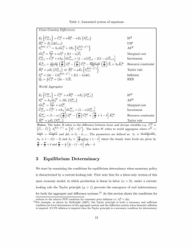
Table 1: Linearized system of equations

Cross-Country Differences

Et

{CRt+1

}= CRt + σRRt − σEt

{πRt+1

}ISR

RRt = Et {∆et+1} UIP

πR(h−f∗)t = Λ1mc

Rt + βEt

{πR(h−f∗)t+1

}ASR

mcRt =

CRt

σ+ αxRt + 2(1 − a)Tt Marginal cost

CRt+1 = CRt + σΛ2

[mc

Rt+1 + (1 − α)xRt+1 − 2(1 − a)Tt+1

]Investment

KRt+1 = (1−α)

(2a−1)

(Z

K

)xRt −

(C

K

)CRt − 4θa(1−a)

(2a−1)

(Z

K

)Tt + Λ3K

Rt Resource constraint

RRt = µEt{πRt+v

}or RRt = µEt

{πR(h−f∗)t+v

}Taylor rule

πRt = (2a− 1)πR(h−f∗)t + 2(1 − a)∆et Inflation

Qt = 1σCRt = (2a− 1)Tt RER

World Aggregates

Et

{CWt+1

}= CWt + σRWt − σEt

{πWt+1

}ISW

πWt = Λ1mcWt + βEt

{πWt+1

}ASW

mcWt =

CWt

σ+ αxWt Marginal cost

CWt+1 = CWt + σΛ2

[mc

Wt+1 + (1 − α)xWt+1

]Investment

KWt+1 = (1 − α)

(Z

K

)xWt −

(C

K

)CWt +

[Z

K+ 1 − δ

]KWt Resource constraint

RWt = µEt{πWt+v

}Taylor rule

Notes: The index R refers to the difference between home and foreign variables e.g. CRt ≡(

Ct − C∗t

), π

R(h−f∗)t ≡

(πht − π

∗ft

). The index W refers to world aggregates where πW =

π+π∗

2= πh+π∗f

2and ∆et ≡ et − et−1. The parameters are defined as: Λ1 ≡

(1−ψ)(1−βψ)ψ

,

Λ2 ≡ 1 − β(1 − δ) and Λ3 =[Z

K

1(2a−1)

+ 1 − δ]

where the steady state levels are given by

Z

K= C

K+ δ and C

K= 1

α

[1β− (1 − δ)

]λλ−1

− δ.

3 Equilibrium Determinacy

We start by examining the conditions for equilibrium determinacy when monetary policy

is characterized by a current-looking rule. First note that for a labor-only version of this

open economy model, in which production is linear in labor (α = 0), under a current-

looking rule the Taylor principle (µ > 1) prevents the emergence of real indeterminacy

for both the aggregate and difference systems.12 As this section shows the conditions for

reduces to the relative PPP condition for consumer price inflation i.e. πRt = ∆et.12For example, as shown by McKnight (2007), the Taylor principle is both a necessary and sufficient

condition for local determinacy of the aggregate system and the difference system when domestic inflationis targeted. If CPI inflation is targeted then the Taylor principle is a necessary condition for determinacy

12

determinacy alter substantially with the inclusion of capital.

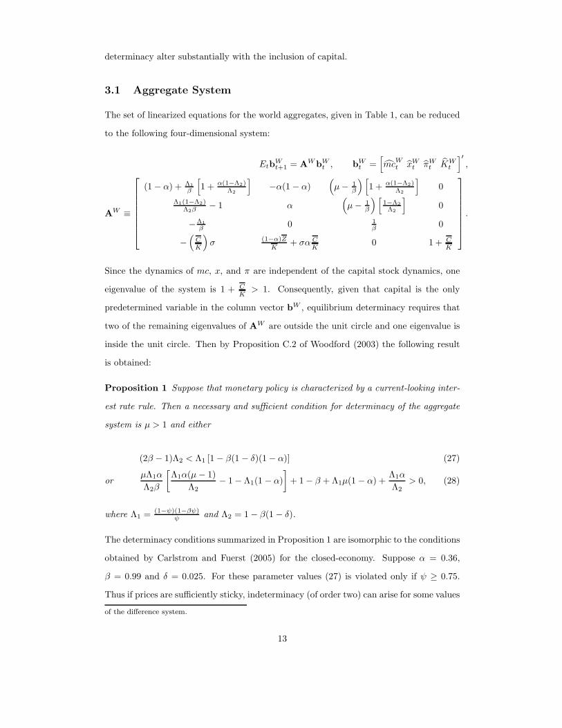
3.1 Aggregate System

The set of linearized equations for the world aggregates, given in Table 1, can be reduced

to the following four-dimensional system:

EtbWt+1 = AWbWt , bWt =

[mc

Wt xWt πWt KW

t

]′

,

AW ≡

(1 − α) + Λ1

β

[1 + α(1−Λ2)

Λ2

]−α(1 − α)

(µ− 1

β

) [1 + α(1−Λ2)

Λ2

]0

Λ1(1−Λ2)Λ2β

− 1 α(µ− 1

β

) [1−Λ2

Λ2

]0

−Λ1

β0 1

β0

−(C

K

)σ (1−α)Z

K+ σα C

K0 1 + C

K

.

Since the dynamics of mc, x, and π are independent of the capital stock dynamics, one

eigenvalue of the system is 1 + C

K> 1. Consequently, given that capital is the only

predetermined variable in the column vector bW , equilibrium determinacy requires that

two of the remaining eigenvalues of AW are outside the unit circle and one eigenvalue is

inside the unit circle. Then by Proposition C.2 of Woodford (2003) the following result

is obtained:

Proposition 1 Suppose that monetary policy is characterized by a current-looking inter-

est rate rule. Then a necessary and sufficient condition for determinacy of the aggregate

system is µ > 1 and either

(2β − 1)Λ2 < Λ1 [1 − β(1 − δ)(1 − α)] (27)

orµΛ1α

Λ2β

[Λ1α(µ− 1)

Λ2− 1 − Λ1(1 − α)

]+ 1 − β + Λ1µ(1 − α) +

Λ1α

Λ2> 0, (28)

where Λ1 = (1−ψ)(1−βψ)ψ

and Λ2 = 1 − β(1 − δ).

The determinacy conditions summarized in Proposition 1 are isomorphic to the conditions

obtained by Carlstrom and Fuerst (2005) for the closed-economy. Suppose α = 0.36,

β = 0.99 and δ = 0.025. For these parameter values (27) is violated only if ψ ≥ 0.75.

Thus if prices are sufficiently sticky, indeterminacy (of order two) can arise for some values

of the difference system.

13

of µ > 1 provided condition (28) is violated. However the region of indeterminacy is small.

For example if ψ = 0.8 then indeterminacy arises provided 1.1 < µ < 1.71, whereas if

ψ = 0.75 condition (28) is satisfied ∀µ > 1 and thus indeterminacy is not possible.

3.2 Difference System

3.2.1 Domestic Price Inflation

If domestic price inflation is the policy indicator, then the set of linearized conditions for

cross-country differences yields a system of the form:

EtbRt+1 = AR

PPIbRt , bRt =

[mcRt xRt π

R(h−f∗)t KR

t

]′

,

ARPPI ≡

1 − α(2a− 1) + Λ1

βJ1 α2(2a− 1) − α

(µ− 1

β

)J1 0

−(2a− 1) + Λ1

βJ2 α(2a− 1)

(µ− 1

β

)J2 0

−Λ1

β0 1

β0

−[σ(2a− 1)C

K+ 4θa(1−a)

(2a−1)Z

K

]J3 0 1 +

C

K+δ2(1−a)

(2a−1)

,

where J1 =[1 + α(1−Λ2)(2a−1)

Λ2

]J2 = (1−Λ2)(2a−1)

Λ2and J3 = (1−α)

(2a−1)Z

K[1 + α4θa(1 − a)] +

σα(2a−1)CK

. As before, the capital stock dynamics can be decoupled from the rest of the

system. However, the eigenvalue associated with the capital stock dynamics now depends

on the degree of trade openness. Consequently this eigenvalue can be either inside or

outside the unit circle depending on the value of a. The Appendix proves the following:13

Proposition 2 Suppose that monetary policy reacts to current-looking domestic price

inflation. Then for an active monetary policy (µ > 1), the necessary and sufficient con-

ditions for determinacy of the difference system are:

(Case I) a > 0.5 and either

(2β − 1)Λ2 < Λ1 [1 − β(1 − δ)(1 − (2a− 1)α)] (29)

orµΛ4

Λ2β

[Λ4(µ− 1)

Λ2+ Λ4 − (1 + Λ1 + Λ2β)

]+ (1 − β) + Λ1µ+

Λ4

Λ2> 0; (30)

13While determinacy of the difference system can also be achieved under a passive monetary policy (µ < 1),such conditions are not reported since the aggregate system is always indeterminate (from Proposition1).

14

(Case II) 0.5 > a >1

2 − δ

[1 − δ −

C

K

1

2

]

and 1 + µ <2(1 + β)Λ2

Λ1 [(1 − 2a)α(2 − Λ2) − Λ2]if

2α(1 − 2a)

1 + α(1 − 2a)> Λ2;

(Case III) a <1

2 − δ

[1 − δ −

C

K

1

2

]< 0.5 and (31)

(i) 1 + µ >2(1 + β)Λ2

Λ1 [(1 − 2a)α(2 − Λ2) − Λ2]and (ii)

2α(1 − 2a)

1 + α(1 − 2a)> Λ2. (32)

where Λ1 = (1−ψ)(1−βψ)ψ

, Λ2 = 1 − β(1 − δ) and Λ4 = Λ1α(2a− 1).

Proof. See Appendix A.1. �

Cases I and II of Proposition 2 show the regions of determinacy when the root associ-

ated with the capital stock dynamics is unstable, whereas Case III shows the regions of

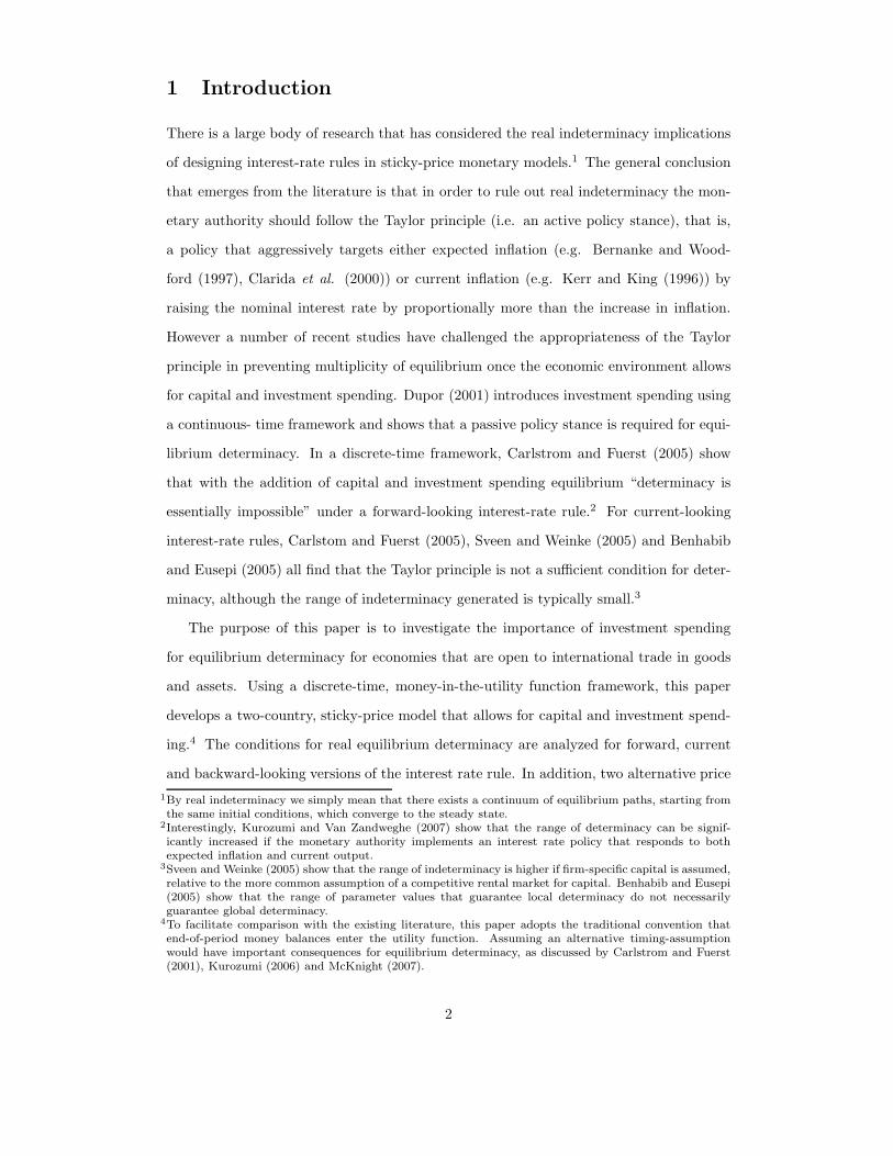
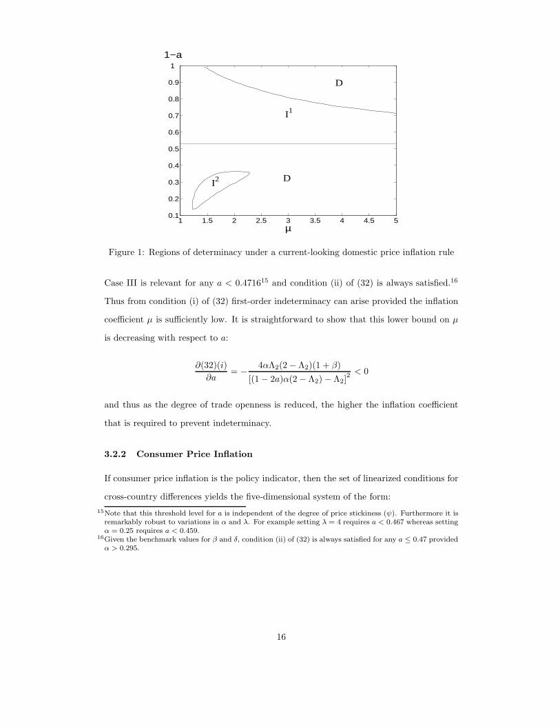
determinacy when this root is stable. We illustrate these determinacy conditions using

the following parameter values. Suppose α = 0.36, β = 0.99, δ = 0.025, λ = 7.66 and

ψ = 0.75. Figure 1 depicts the regions in the parameter space (a, µ) that are associated

with determinacy (D), first-order indeterminacy (I1) and second-order indeterminacy (I2)

around the neighborhood of the steady state.14 If the degree of trade openness is suf-

ficiently low (a > 0.5) then second-order indeterminacy can arise in the open-economy.

This follows from the violation of conditions (29) and (30) of Case I in Proposition 2.

Indeed comparing (29) with condition (27) of Proposition 1 yields

(2β − 1)Λ2 < Λ1 [1 − β(1 − δ)(1 − (2a− 1)α)] < Λ1 [1 − β(1 − δ)(1 − α)] ,

which by inspection implies that a higher degree of price stickiness is required in the

open economy to prevent the emergence of second-order indeterminacy. Furthermore, as

depicted in Figure 1, if the degree of trade openness is sufficiently high then first-order

indeterminacy can also exist. This arises from the violation of condition (32) of Case III

in Proposition 2. First consider condition (31). Under the assigned parameter values,

14Recall that with these parameter values indeterminacy is not possible in the closed-economy (aggregatesystem) ∀µ > 1.

15

1 1.5 2 2.5 3 3.5 4 4.5 50.1

0.2

0.3

0.4

0.5

0.6

0.7

0.8

0.9

1

µ

1−a

D

I1

D

I2

Figure 1: Regions of determinacy under a current-looking domestic price inflation rule

Case III is relevant for any a < 0.471615 and condition (ii) of (32) is always satisfied.16

Thus from condition (i) of (32) first-order indeterminacy can arise provided the inflation

coefficient µ is sufficiently low. It is straightforward to show that this lower bound on µ

is decreasing with respect to a:

∂(32)(i)

∂a= −

4αΛ2(2 − Λ2)(1 + β)

[(1 − 2a)α(2 − Λ2) − Λ2]2 < 0

and thus as the degree of trade openness is reduced, the higher the inflation coefficient

that is required to prevent indeterminacy.

3.2.2 Consumer Price Inflation

If consumer price inflation is the policy indicator, then the set of linearized conditions for

cross-country differences yields the five-dimensional system of the form:

15Note that this threshold level for a is independent of the degree of price stickiness (ψ). Furthermore it isremarkably robust to variations in α and λ. For example setting λ = 4 requires a < 0.467 whereas settingα = 0.25 requires a < 0.459.

16Given the benchmark values for β and δ, condition (ii) of (32) is always satisfied for any a ≤ 0.47 providedα > 0.295.

16

EtbRt+1 = AR

CPIbRt , bRt =

[mc

Rt xRt πRt−1 π

Rt KR

t

]′

, and ARCPI ≡

1 − α(2a− 1) + Λ1(1+αJ1)β

α2(2a− 1) − α J2(1 + αJ1) J3(1 + αJ1) 0

−(2a− 1) + Λ1

βJ1 α(2a− 1) J2J1 J3J1 0

0 0 0 1 0

−Λ1(2a−1)β

0 − 2(1−a)µβ

1+2(1−a)βµβ

0

−[σ(2a−1)C

K+ 4θa(1−a)

(2a−1)Z

K

]J4 0 0 1 +

C

K+δ2(1−a)

(2a−1)

,

where J1 = (1−Λ2)(2a−1)Λ2

, J2 = 2(1−a)µ(2a−1)β , J3 = µ− 1

β(2a−1) and J4 = (1−α)(2a−1)

Z

K[1 + α4θa(1 − a)]+

σα(2a − 1)CK

. Now there are two predetermined variables KRt and πRt−1. Note that the

eigenvalue associated with the capital stock dynamics is the same regardless of the index

of inflation targeted. The Appendix proves the following:

Proposition 3 Suppose that monetary policy reacts to current-looking consumer price

inflation. Then for an active monetary policy (µ > 1), the necessary and sufficient con-

ditions for determinacy of the difference system are:

(Case I) a > 0.5 and at least one of (33) and (34) is satisfied;

µ >(2β − 1)Λ2 − Λ1 [Λ2 + α(1 − Λ2)(2a− 1)]

Λ2β2(1 − a), (33)

µ

β

[2(1 − a) +

Λ4

Λ2

] [2(1 − a)(1 − β)µ+

Λ4[µ− (1 − Λ2)]

Λ2− (1 + Λ1)

]

+ (1 − β) + µ [Λ1 − Λ4] + 2(1 − a)µβ +Λ4

Λ2> 0; (34)

(Case II) 0.5 > a >1

2 − δ

[1 − δ −

C

K

1

2

], and

Λ1 <2Λ2(1 + β)[1 + 2µ(1 − a)]

(1 + µ) [α(1 − 2a)(2 − Λ2) − Λ2]if

2α(1 − 2a)

1 + α(1 − 2a)> Λ2, (35)

and at least one of (33) and (34) is satisfied;

17

(Case III) a <1

2 − δ

[1 − δ −

C

K

1

2

]< 0.5, and

Λ1 >2Λ2(1 + β)[1 + 2µ(1 − a)]

(1 + µ) [α(1 − 2a)(2 − Λ2) − Λ2]and (36)

Λ2 < min

{2α(1 − 2a)

1 + α(1 − 2a),Λ1α(1 − 2a)

2(1 − a)

}; (37)

where Λ1 = (1−ψ)(1−βψ)ψ

, Λ2 = 1 − β(1 − δ) and Λ4 = Λ1α(2a− 1).

Proof. See Appendix A.2. �

Comparison of Propositions 2 and 3 highlight important qualitative differences between

reacting to consumer and domestic price inflation. First, the range of second-order in-

determinacy is relatively lower if consumer price inflation is targeted. This follows from

direct comparison of conditions (29) and (33):

(2β − 1)Λ2 < Γ1 < 2βΛ2(1 − a)µ+ Γ1,

where Γ1 = Λ1 [1 − β(1 − δ)(1 − (2a− 1)α)]. Secondly, the range of first-order indeter-

minacy is relatively greater under consumer price inflation targeting. By comparing the

Case III conditions of Propositions 2 and 3, it is straightforward to show that (36) is a

stronger requirement for determinacy than condition (i) of (32).17 Furthermore by com-

paring condition (ii) of (32) with (37), reacting to consumer price inflation introduces an

additional determinacy condition given by Λ2 <Λ1α(1−2a)

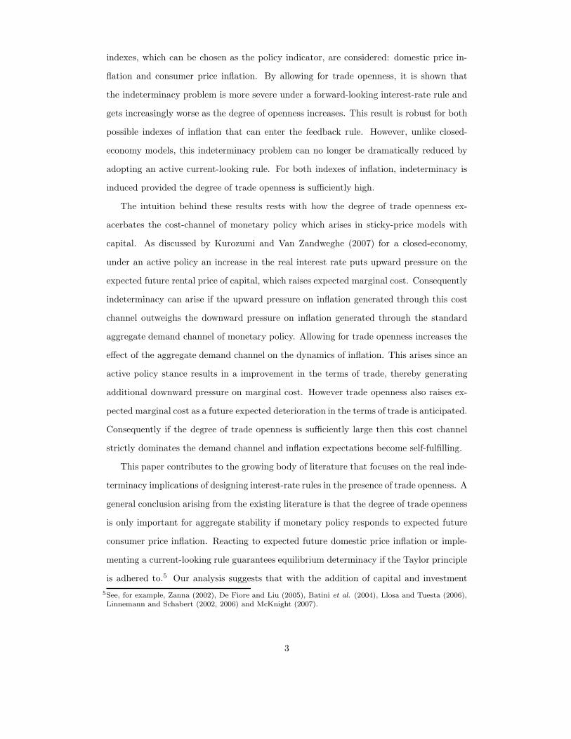
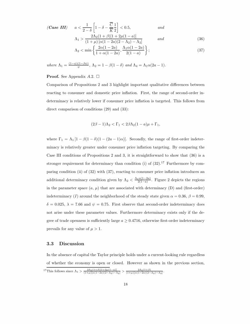
2(1−a) . Figure 2 depicts the regions

in the parameter space (a, µ) that are associated with determinacy (D) and (first-order)

indeterminacy (I) around the neighborhood of the steady state given α = 0.36, β = 0.99,

δ = 0.025, λ = 7.66 and ψ = 0.75. First observe that second-order indeterminacy does

not arise under these parameter values. Furthermore determinacy exists only if the de-

gree of trade openness is sufficiently large a ≥ 0.4716, otherwise first-order indeterminacy

prevails for any value of µ > 1.

3.3 Discussion

In the absence of capital the Taylor principle holds under a current-looking rule regardless

of whether the economy is open or closed. However as shown in the previous section,

17This follows since Λ1 >2Λ2(1+β)[1+2µ(1−a)]

(1+µ)[α(1−2a)(2−Λ2)−Λ2]>

2Λ2(1+β)(1+µ)[α(1−2a)(2−Λ2)−Λ2]

.

18

1 1.5 2 2.5 3 3.5 4 4.5 50

0.1

0.2

0.3

0.4

0.5

0.6

0.7

0.8

0.9

1

µ

1−a

D

I

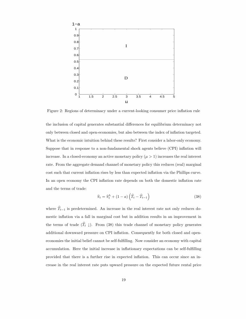
Figure 2: Regions of determinacy under a current-looking consumer price inflation rule

the inclusion of capital generates substantial differences for equilibrium determinacy not

only between closed and open-economies, but also between the index of inflation targeted.

What is the economic intuition behind these results? First consider a labor-only economy.

Suppose that in response to a non-fundamental shock agents believe (CPI) inflation will

increase. In a closed-economy an active monetary policy (µ > 1) increases the real interest

rate. From the aggregate demand channel of monetary policy this reduces (real) marginal

cost such that current inflation rises by less than expected inflation via the Phillips curve.

In an open economy the CPI inflation rate depends on both the domestic inflation rate

and the terms of trade:

πt = πht + (1 − a)(Tt − Tt−1

)(38)

where Tt−1 is predetermined. An increase in the real interest rate not only reduces do-

mestic inflation via a fall in marginal cost but in addition results in an improvement in

the terms of trade (Tt ↓). From (38) this trade channel of monetary policy generates

additional downward pressure on CPI inflation. Consequently for both closed and open-

economies the initial belief cannot be self-fulfilling. Now consider an economy with capital

accumulation. Here the initial increase in inflationary expectations can be self-fulfilling

provided that there is a further rise in expected inflation. This can occur since an in-

crease in the real interest rate puts upward pressure on the expected future rental price

19

of capital (from the investment condition (18)) which leads to an increase in expected

future marginal cost and thus an additional rise in expected future inflation. Therefore

indeterminacy is generated if the effect of this cost channel of monetary policy is suffi-

ciently strong to counteract the downward pressure on inflation arising from the aggregate

demand channel. In the open-economy the increase in expected future marginal cost is

exacerbated as the degree of trade openness increases. This strengthens the effect of the

cost channel making a rise in domestic price inflation more likely. From (38) there are

two opposing effects on CPI inflation, the strength of both are increasing as the degree

of trade openness increases (a ↓). Therefore depending on the size of a this determines

which effect dominates and thus whether the initial inflationary belief is validated.

4 The Timing of Interest-rate Rules

So far the analysis has focused on interest-rate rules that target contemporaneous infla-

tion. In this section we consider interest-rate rules that react to either forward-looking or

backward-looking inflation.

4.1 Forward-looking rules

We start by examining the conditions for equilibrium determinacy under forward-looking

inflation rules. The aggregate and difference systems are both four-dimensional generating

a zero eigenvalue in each case. Since capital is the only predetermined variable, equilibrium

determinacy requires the remaining three eigenvalues to lie outside the unit circle. This

automatically suggests that for determinacy of the difference system, the root associated

with the capital stock dynamics must be unstable, which in turn implies that determinacy

is impossible for sufficiently open economies.

4.1.1 Aggregate System

Under a forward-looking rule, the set of linearized equations for the world aggregates,

given in Table 1, yields a system of the form:

20

EtbWt+1 = BWbWt , bWt =

[mc

Wt xWt πWt KW

t

]′

,

BW ≡

(1 − α) − Λ1(µ−1)[α+Λ2(1−α)]βΛ2

−α(1 − α) (µ−1)[α+Λ2(1−α)]βΛ2

0

−1 − (µ−1)Λ1(1−Λ2)βΛ2

α (µ−1)(1−Λ2)βΛ2

0

−Λ1

β0 1

β0

−(C

K

)σ (1 − α) Z

K+ σα C

K0 1 + C

K

.

One eigenvalue of the system is given by 1 + C

K> 1, while another eigenvalue is zero.

Consequently, equilibrium determinacy requires that the two remaining eigenvalues of BW

are outside the unit circle. Then by Proposition C.1 of Woodford (2003) the following

result is obtained:

Proposition 4 Suppose that monetary policy is characterized by a forward-looking inter-

est rate rule. Then a necessary and sufficient condition for determinacy of the aggregate

system is

1 < µ < 1 + min

{ΓA1 ≡

(1 − β)Λ2

αΛ1,ΓA2 ≡

2(1 + β)Λ2

Λ1 [α(2 − Λ2) + Λ2]

}(39)

where Λ1 = (1−ψ)(1−βψ)ψ

and Λ2 = 1 − β(1 − δ).

As discussed by Carlstrom and Fuerst (2005) the regions of determinacy for a closed-

economy are remarkably narrow under a forward-looking rule with capital.18 Again sup-

pose that α = 0.36, β = 0.99 and δ = 0.025. Then the upper bound for determinacy is

1.01124 = ΓA1 < ΓA2 . Propositions 5 and 6 below show that in an open-economy the range

of determinacy is even smaller.

4.1.2 Difference System

The set of linearized conditions for cross-country differences yields a system of the form:

18Carlstrom and Fuerst (2005) present a necessary condition for determinacy, whereas Proposition 4 providesa necessary and sufficient condition for determinacy.

21

EtbRt+1 = BRbRt , bt =

[mc

Rt xRt π

R(h−f∗)t KR

t

]′

,

BR ≡

1 − α(2a− 1) − Λ1J1 α2(2a− 1) − α J1 0

−(2a− 1) − Λ1J2 α(2a− 1) J2 0

−Λ1

β0 1

β0

−[σ(2a− 1)C

K+ 4θa(1−a)

(2a−1)Z

K

]J3 0 1 + 1

(2a−1)

[C

K+ δ2(1 − a)

]

,

where J1 = (µ−1)β

[1 + α(1−Λ2)(2a−1)

Λ2

]and J2 = (µ−1)(1−Λ2)(2a−1)

βΛ2under domestic inflation

targeting; whereas J1 =(µ−1)(2a−1)[α(1−Λ2)+

Λ2(2a−1) ]

βΛ2[1−2(1−a)µ] and J2 = (µ−1)(1−Λ2)(2a−1)βΛ2[1−2(1−a)µ] under CPI

inflation targeting. Finally J3 = (1−α)(2a−1)

Z

K[1 + α4θa(1 − a)] + σα(2a − 1)C

K. Analogous

to the aggregate system, one eigenvalue of the system is zero. Therefore determinacy

requires the eigenvalue 1 + 1(2a−1)

[C

K+ δ2(1 − a)

]to have a modulus greater than one,

and the two remaining eigenvalues of BR are also outside the unit circle. By Proposition

C.1 of Woodford (2003) the following results are obtained:

Proposition 5 Suppose that monetary policy reacts to forward-looking domestic price

inflation. Then for an active monetary policy (µ > 1), the necessary and sufficient con-

ditions for determinacy of the difference system are

(Case I) a > 0.5 and

1 < µ < 1 + min

{ΓB1 ≡

(1 − β)Λ2

αΛ1(2a− 1)ΓA2 ≡

2(1 + β)Λ2

Λ1α(2 − Λ2)(2a− 1)

}; (40)

(Case II) 0.5 > a >1

2 − δ

[1 − δ −

C

K

1

2

]; (41)

where Λ1 = (1−ψ)(1−βψ)ψ

and Λ2 = 1 − β(1 − δ).

Proposition 6 Suppose that monetary policy reacts to forward-looking consumer price

inflation. Then for an active monetary policy (µ > 1), the necessary and sufficient con-

22

ditions for determinacy of the difference system are

(Case I) a > 0.5 and 1 < µ < min

{ΓC1 ,Γ

C2 ,Γ

C3

}; (42)

(Case II) 0.5 > a >1

2 − δ

[1 − δ −

C

K

1

2

]and (43)

2(1 + β) +(µ− 1)Λ1

Λ2 (2µ(1 − a) − 1)[Λ2 − 2α(1 − 2a) (2 − Λ2)] < 0;

where ΓC1 ≡ 12(1−a) , ΓC2 ≡ (1−β)Λ2+Λ1α(2a−1)

Λ1α(2a−1)+(1−β)Λ22(1−a) , ΓC3 ≡ 2(1+β)Λ2+Λ1[Λ2+(2a−1)α(2−Λ2)]4(1+β)(1−a)Λ2+Λ1[Λ2+(2a−1)α(2−Λ2)] .

Suppose α = 0.36, β = 0.99, δ = 0.025 and λ = 7.66. Given the assigned parameter

values conditions (41) and (43) of Propositions 5 and 6 are violated if a < 0.4716 and thus

(first-order) indeterminacy arises ∀µ > 1. If a > 0.5 then under domestic price inflation

targeting the open-economy introduces no additional requirements for determinacy. This

follows by direct comparison of the upper bounds on µ given by conditions (39) and (40):

ΓA1 < ΓB1 and ΓA2 < ΓB2 . However if a > 0.5 and consumer price inflation is targeted then

comparing (39) with (42) yields ΓC2 < ΓA1 and ΓC3 < ΓA2 . Since ∂ΓCi /∂a > 0 for i = 1, 2, 3,

the inflation coefficient µ is constrained by these upper bounds, all of which are increasing

with respect to a. Thus the range of indeterminacy is potentially greater the higher the

degree of trade openness (i.e. the lower is a).

As discussed by Kurozumi and Van Zandweghe (2007) in a closed economy an active

forward-looking policy makes inflation expectations self-fulfilling entirely because of the

cost channel of monetary policy. However in the open-economy indeterminacy is more

severe because of the additional impact the trade channel has on inflation. Under an active

forward-looking policy, the increase in the real interest rate results in a future expected

deterioration in the terms of trade (Tt+1 increases relative to Tt). Thus the trade effect

puts upward

Etπt+1 = Etπht+1 + (1 − a)

(EtTt+1 − Tt

)

pressure on inflation, the effect of which is stronger the higher the degree of trade openness

(a ↓).

23

4.2 Backward-looking rules

We now turn our attention to backward-looking interest-rate rules. The determinacy

analysis proceeds as before except now the aggregate system is five-dimensional and de-

terminacy requires two eigenvalues to lie inside the unit circle and the remaining three

eigenvalues be outside the unit circle. The difference system is six-dimensional under con-

sumer price inflation targeting and determinacy therefore requires that there are exactly

three eigenvalues inside the unit circle and three eigenvalues outside the unit circle. As

before the capital dynamics eigenvalue can lie inside or outside the unit circle depending

on the size of a. Since responding to backward inflation makes the analytical conditions

for determinacy more complex to derive, we will simply report some numerical results.

Suppose α = 0.36, β = 0.99 and δ = 0.025. Then determinacy of the aggregate system

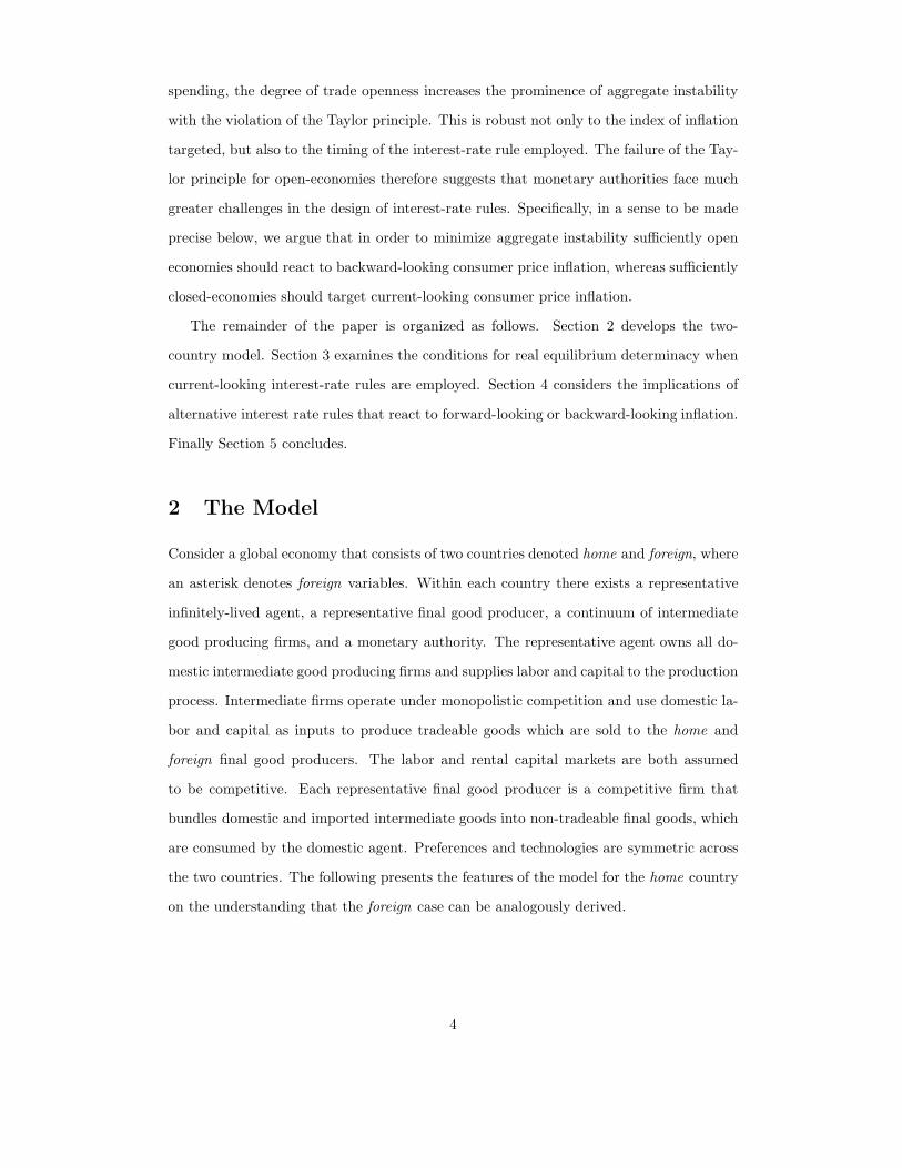
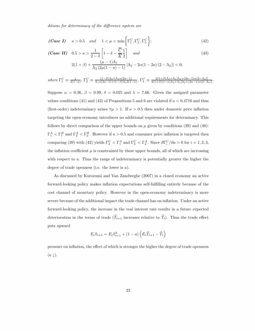
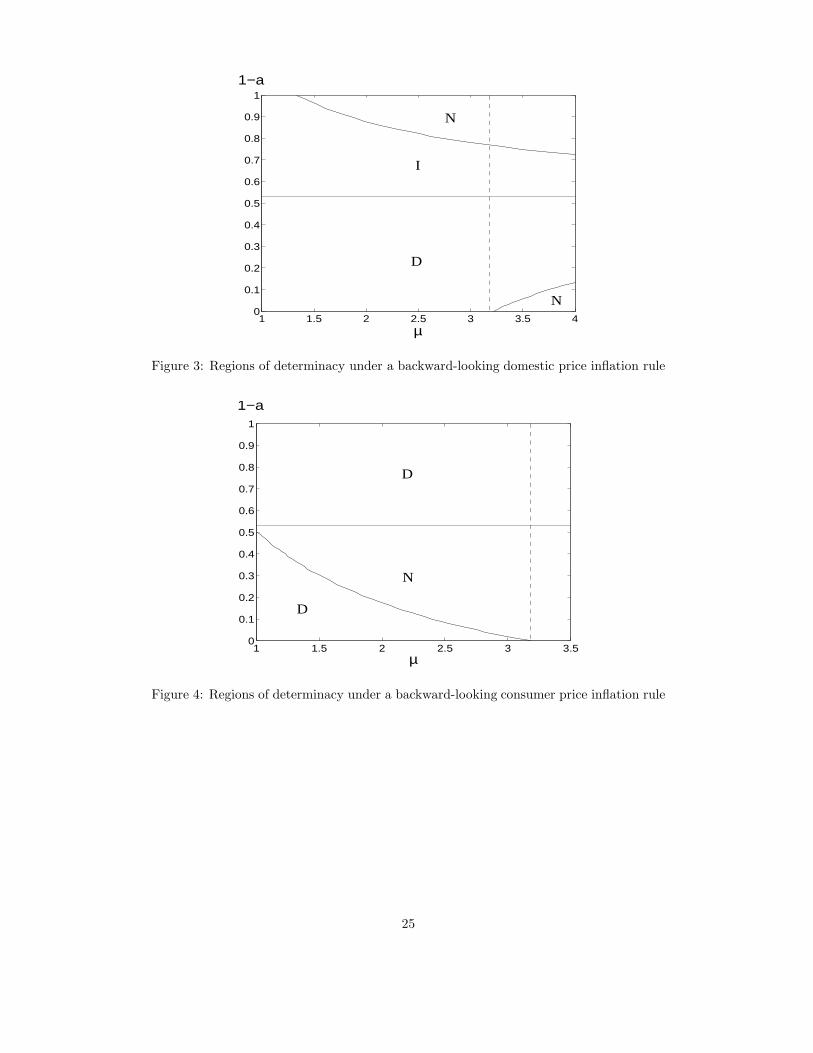
requires that 1 < µ < 3.171 otherwise no equilibrium exists. Figures 3 and 4 depict the

regions in the parameter space (a, µ) that are associated with determinacy (D), (first-

order) indeterminacy (I) and an explosive solution (N) around the neighborhood of the

steady state, for both possible indexes of inflation. First consider the case when the

capital dynamics root is unstable (a ≥ 0.4716). Inspection of figure 3 suggests that if

domestic price inflation is targeted the open-economy places no additional restrictions for

equilibrium determinacy. However if consumer price inflation is targeted, figure 4 sug-

gests that the upper bound on the inflation coefficient is more severe in the open-economy.

Furthermore the range of determinacy decreases as the degree of trade openness increases

therefore implying that this upper bound is increasing with respect to a. Next consider

the case where the eigenvalue associated with the capital dynamics lies inside the unit cir-

cle (a < 0.4716). If domestic price inflation is targeted then determinacy is not possible,

whereas if consumer price inflation is targeted determinacy prevails.

24

1 1.5 2 2.5 3 3.5 40

0.1

0.2

0.3

0.4

0.5

0.6

0.7

0.8

0.9

1

µ

1−a

D

I

N

N

Figure 3: Regions of determinacy under a backward-looking domestic price inflation rule

1 1.5 2 2.5 3 3.50

0.1

0.2

0.3

0.4

0.5

0.6

0.7

0.8

0.9

1

µ

1−a

D

N

D

Figure 4: Regions of determinacy under a backward-looking consumer price inflation rule

25

The above analysis suggests that in the presence of capital there are important im-

plications for equilibrium determinacy depending on whether the economy is open or

closed. In a closed-economy, indeterminacy can easily be prevented by avoiding forward-

looking interest-rate rules. However in open-economies implementing current-looking or

backward-looking policies is contingent upon the degree of trade openness of the econ-

omy in question. For sufficiently closed economies, the monetary authority should adopt

a current-looking CPI interest-rate rule to minimize policy-induced aggregate instabil-

ity. However for economies that are sufficiently open to trade a backward-looking CPI

interest-rate rule is a more appropriate policy.

5 Conclusion

This paper has considered the importance of trade openness for equilibrium determinacy

in the presence of capital and investment spending. It has been shown that policy in-

duced indeterminacy is considerably easier to obtain using a sticky-price open-economy

model compared to its closed-economy variant. This conclusion is robust to the index of

inflation chosen as the policy indicator and the timing of the interest-rate rule employed.

The analysis suggests that considerable care needs to be taken when designing interest-

rate rules for economies that actively engage in cross-country trade. Adopting policies

advocated for closed-economies, may not be sufficient to prevent the emergence of real

indeterminacy.

26

References

[1] Aoki, M. 1981. Dynamic Analysis of Open Economies. New York: Academic Press.

[2] Batini, N., P. Levine and J. Pearlman, 2004. Indeterminacy with Inflation-Forecast-

Based Rules in a Two-Bloc Model. International Finance Discussion Paper No. 797,

Board of Governors of the Federal Reserve System.

[3] Benhabib, J. and S. Eusepi, 2005. The Design of Monetary and Fiscal Policy: A Global

Perspective. Journal of Economic Theory 123, pp40-73.

[4] Bernanke, B. and M. Woodford, 1997. Inflation Forecast and Monetary Policy, Part

2. Journal of Money, Credit and Banking 29, pp653-684.

[5] Calvo, G., 1983. Staggered Prices in a Utility Maximising Framework. Journal of

Monetary Economics 12, pp983-998.

[6] Carlstrom, C.T. and T.S. Fuerst, 2001. Timing and Real Indeterminacy in Monetary

Models. Journal of Monetary Economics 47, pp285-298.

[7] Carlstrom, C.T. and T.S. Fuerst, 2005. Investment and Interest Rate Policy: A Dis-

crete Time Analysis. Journal of Economic Theory 123, pp4-20.

[8] Clarida, R., J. Gali, and M. Gertler, 2000. Monetary Policy Rules and Macroeconomic

Stability: Evidence and Some Theory. Quarterly Journal of Economics 115, pp147-

180.

[9] De Fiore, F. and Z. Liu, 2005. Does Trade Openness Matter for Aggregate Instability?

Journal of Economic Dynamics and Control 29, pp1165-1192.

[10] Dupor, B. 2001. Investment and Interest Rate Policy. Journal of Economic Theory

98, pp85-113.

[11] Kerr, W. and R. King, 1996. Limits in Interest-rate Rules in the IS-LM Model.

Federal Reserve Bank of Richmond Economic Quarterly.

[12] Kurozumi, T., 2006. Determinacy and Expectational Stability of Equilibrium in a

Monetary Sticky-Price Model with Taylor Rules, Journal of Monetary Economics 53,

pp827-846.

27

[13] Kurozumi, T. and W. Van Zandweghe 2007. Investment, Interest Rate Policy and

Equilibrium Stability. mimeo.

[14] Linnemann, L. and L. Schabert 2002. Monetary Policy, Exchange Rates and Real

Indeterminacy. mimeo, University of Cologne.

[15] Linnemann, L. and L. Schabert 2006. On the Validity of the Taylor Principle in Open

Economies. mimeo, University of Cologne.

[16] Llosa, G. and V. Tuesta 2006. Determinacy and Learnability of Monetary Policy

Rules in Small Open Economies. mimeo.

[17] McKnight, S., 2007. Real Indeterminacy and the Timing of Money in Open

Economies. mimeo, Department of Economics, University of Reading.

[18] Sveen, T. and L. Weinke, 2005. New Perspectives on Capital, Sticky Prices, and the

Taylor Principle. Journal of Economic Theory 123, pp21-39.

[19] oodford, M., 2003. Interest Rates and Prices: Foundations of a Theory of Monetary

Policy. Princeton: Princeton University Press.

[20] Zanna, L., 2002. Interest Rate Rules and Multiple Equilibria in the Small Open

Economy. mimeo, University of Pennsylvania.

28

A Appendix

A.1 Proof of Proposition 2

As shown in the main text, if monetary policy targets current-looking domestic price

inflation this results in a four dimensional system[mc

Rt xRt π

R(h−f∗)t KR

t

]′

, where KR

is the only predetermined endogenous variable. Determinacy of the difference system

thus requires one eigenvalue to lie inside the unit circle and the other three eigenvalues

to lie outside the unit circle. One eigenvalue of the coefficient matrix ARPPI is given by

eK ≡ 1 + 1(2a−1)

[C

K+ 2δ(1 − a)

], which modulus can be greater or less than one. The

remaining three eigenvalues are determined by the upper left 3 × 3 submatrix of ARPPI ,

denoted by AR

PPI . Then the characteristic equation of AR

PPI is

r3 + a2r2 + a1r + a0 = 0

where

a2 = −1 −1

β−

Λ1

β

[1 +

α(1 − Λ2)(2a− 1)

Λ2

]

a1 =1

β+

Λ1µ

β

[1 +

α(1 − Λ2)(2a− 1)

Λ2

]+αΛ1(2a− 1)

Λ2β

a0 = −Λ1µα(2a− 1)

Λ2β.

First suppose the eigenvalue eK is unstable, |eK | > 1, which requires either a > 0.5 or

0.5 > a > 12−δ

[1 − δ − 1

2C

K

]. Then using Proposition C.2 of Woodford (2003), two of the

remaining three eigenvalues are outside the unit circle and one eigenvalue is inside the

unit circle if and only if: (Case I)

1 + a2 + a1 + a0 > 0 ⇔(µ− 1)Λ1

β[1 − (2a− 1)α] < 0, (A1)

−1 + a2 − a1 + a0 > 0 ⇔ −2(1 + β) − (µ+ 1)Λ1

[1 +

(2a− 1)α(2 − Λ2)

Λ2

]> 0, (A2)

or (Case II)

1 + a2 + a1 + a0 > 0 ⇔(µ− 1)Λ1

β[1 − (2a− 1)α] > 0, (A3)

29

−1 + a2 − a1 + a0 > 0 ⇔ −2(1 + β) − (µ+ 1)Λ1

[1 +

(2a− 1)α(2 − Λ2)

Λ2

]< 0, (A4)

and either

a20 − a0a2 + a1 − 1 > 0, (A5a)

or

|a2| < −3. (A5b)

Assume µ > 1, since otherwise the aggregate system would be indeterminate. Then Case

I is not relevant since condition (A1) is violated by assumption. For Case II, condition

(A3) is satisfied ∀ µ > 1 since 1 − α(2a− 1) > 0. If a > 0.5 then by inspection condition

(A4) is automatically satisfied and either (A5a) or (A5b) is required for determinacy. If

a < 0.5 then condition (A5a) can be derived as:

Λ1α(1 − 2a)µ

Λ2β

[Λ1(1 − 2a)(µ− 1)

Λ2+ Λ1 + Λ2β + (1 − 2a)αΛ1

]

+(1 − β) + Λ1µ+Λ1α(1 − 2a)µ(1 − β)

Λ2β> 0,

which is always satisfied by inspection and thus condition (A5b) does not apply. Fi-

nally condition (A4) is automatically satisfied provided (1−2a)α(2−Λ2)Λ2

< 1. Otherwise the

following upper bound on µ is required: µ < 2(1+β)Λ2

Λ1[(1−2a)α(2−Λ2)−Λ2] − 1.

Now suppose that the eigenvalue eK is stable, |eK | < 1 which requires a < 12−δ

[1 − δ − 1

2C

K

]<

0.5. Determinacy then requires that the remaining three eigenvalues be outside the unit

circle. From the characteristic equation of AR

PPI this implies that r(0) = Λ1µα(1−2a)Λ2β

> 0.

If µ > 1 then r(1) = (µ−1)Λ1

β[1 + α(1 − 2a)] > 0. Therefore if r(−1) > 0 then

the three roots, either real or complex, are outside the unit circle. Since r(−1) =

−2(1+β)−Λ1(µ+1)[1 − α(1−2a)(2−Λ2)

Λ2

], then r(−1) > 0 provided α(1−2a)(2−Λ2) > Λ2

and 1 + µ > 2(1+β)Λ2

Λ1[α(1−2a)(2−Λ2)−Λ2] . This completes the proof. �

A.2 Proof of Proposition 3

If monetary policy targets current-looking consumer price inflation then one eigenvalue of

the coefficient matrix ARCPI is given by eK ≡ 1 + 1

(2a−1)

[C

K+ 2δ(1 − a)

]. The remaining

30

four eigenvalues are determined by the upper left 4 × 4 submatrix of ARCPI , denoted by

AR

CPI . Then the characteristic equation of AR

CPI is

r(r3 + a3r

2 + a2r + a1

)= 0

where

a3 = −1 −1

β−

Λ1

β

[1 +

α(1 − Λ2)(2a− 1)

Λ2

]− 2(1 − a)µ

a2 =1

β+

Λ1µ

β

[1 +

α(1 − Λ2)(2a− 1)

Λ2

]+αΛ1(2a− 1)

Λ2β+

2(1 − a)µ(1 + β)

β

a1 = −µ

β

[2(1 − a) +

Λ1α(2a− 1)

Λ2

].

Hence one eigenvalue is zero and the three remaining eigenvalues are the solutions to the

cubic equation r3 +a3r2 +a2r+a1 = 0. Determinacy requires two eigenvalues to lie inside

the unit circle and the other three eigenvalues to lie outside the unit circle. First suppose

the eigenvalue eK is outside the unit circle |eK | > 1, which requires either a > 0.5 or

0.5 > a > 12−δ

[1 − δ − 1

2C

K

]. Then using Proposition C.2 of Woodford (2003), two of the

remaining three eigenvalues are outside the unit circle and one eigenvalue is inside the

unit circle if and only if: (Case I)

1 + a3 + a2 + a1 > 0 ⇔(µ− 1)Λ1

β[1 − (2a− 1)α] < 0, (B1)

−1+a3−a2+a1 > 0 ⇔ −2(1+β)−4µ(1−a)(1+β)−(µ+1)Λ1

[1 +

(2a− 1)α(2 − Λ2)

Λ2

]> 0,

(B2)

or (Case II)

1 + a3 + a2 + a1 > 0 ⇔(µ− 1)Λ1

β[1 − (2a− 1)α] > 0, (B3)

−1+a3−a2+a1 > 0 ⇔ −2(1+β)−4µ(1−a)(1+β)−(µ+1)Λ1

[1 +

(2a− 1)α(2 − Λ2)

Λ2

]< 0,

(B4)

and either

a21 − a1a3 + a2 − 1 > 0, (B5a)

31

or

|a3| < −3. (B5b)

Assume µ > 1, or otherwise the aggregate system would be indeterminate, then Case

I is not relevant since condition (B1) is violated by assumption. For Case II, condition

(B3) is satisfied ∀µ > 1. If a > 0.5 then by inspection condition (B4) is automatically

satisfied and either (B5a) or (B5b) is required for determinacy. If a < 0.5 condition (B4)

is automatically satisfied provided (1−2a)α(2−Λ2)Λ2

< 1. Otherwise the following condition

is required: Λ1(1 + µ) [α(1 − 2a)(2 − Λ2) − Λ2] < 2Λ2(1 + β)[1 + 2µ(1 − a)]. In addition

either (B5a) or (B5b) is required for determinacy.

Now suppose that the eigenvalue eK is inside the unit circle |eK | < 1, which re-

quires a < 12−δ

[1 − δ − 1

2C

K

]< 0.5. Determinacy then requires that the remaining three

eigenvalues be outside the unit circle. From the characteristic equation of AR

CPI this

implies that r(1) = (µ−1)Λ1

β[1 + α(1 − 2a)] > 0 given the assumption that µ > 1 and

r(0) = −µβ

[2(1 − a) − Λ1α(1−2a)

Λ2

]. This has to be positive r(0) > 0 otherwise there would

be (at least) one stable root, which requires Λ1α(1 − 2a) > 2(1 − a)Λ2. Therefore if

r(−1) > 0 then the three roots, either real or complex, are outside the unit circle. Since

r(−1) = −2(1+β)4µ(1−a)(1+β)−Λ1(µ+1)[1 − α(1−2a)(2−Λ2)

Λ2

], then r(−1) > 0 provided

α(1−2a)(2−Λ2) > Λ2 and Λ1(1+µ) [α(1 − 2a)(2 − Λ2) − Λ2] > 2Λ2(1+β)[1+2µ(1−a)].

This completes the proof. �

32