Economics 173 Business Statistics Lecture 8 Fall, 2001 Professor J. Petry

Economics 173Business Statistics

Lecture 8

Fall, 2001

Professor J. Petry

http://www.cba.uiuc.edu/jpetry/Econ_173_fa01/

2

Inference about the Comparison of

Two Populations

Inference about the Comparison of

Two Populations

Chapter 12

3

12.1 Introduction

• Variety of techniques are presented whose objective is to compare two populations.

• We are interested in:– The difference between two means.– The ratio of two variances.– The difference between two proportions.

4

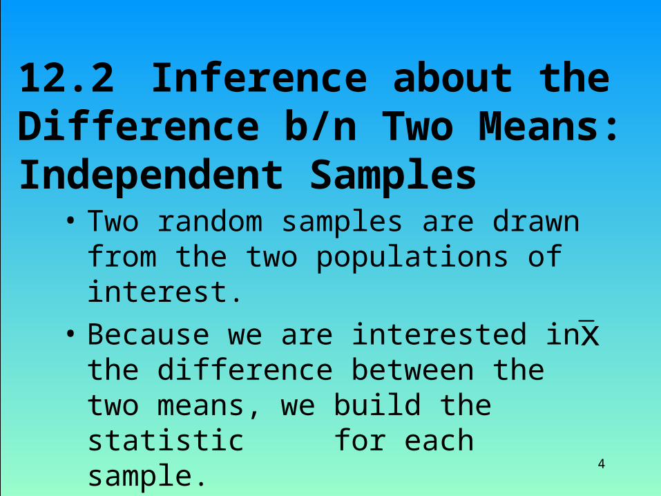
• Two random samples are drawn from the two populations of interest.

• Because we are interested in the difference between the two means, we build the statistic for each sample.

12.2 Inference about the Difference b/n Two Means: Independent Samples

x

5

is normally distributed if the (original) population distributions are normal .

is approximately normally distributed if the (original) population is not normal, but the sample size is large.

Expected value of is 1 - 2

The variance of is 12/n1 + 2

2/n2

21 xx

21 xx

The Sampling Distribution of 21xx

21xx

21xx

6

• If the sampling distribution of is normal or approximately normal we can write:

• Z can be used to build a test statistic or a confidence interval for 1 - 2

21

21

nn

)()xx(Z

21

21

nn

)()xx(Z

21xx

7

• Practically, the “Z” statistic is hardly used, because the population variances are not known.

21

21

nn

)()xx(Z

21

21

nn

)()xx(Z

? ?

• Instead, we construct a “t” statistic using the sample “variances” (S1

2 and S22).

S22S1

2t

8

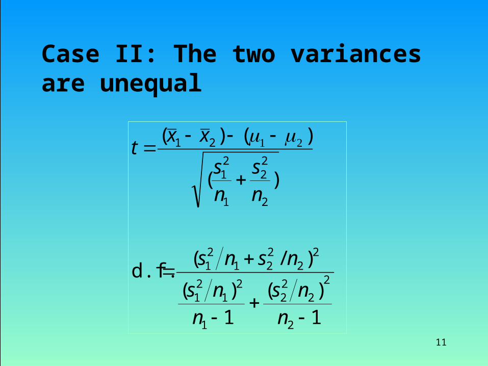
• Two cases are considered when producing the t-statistic.

– The two unknown population variances are equal.

– The two unknown population variances are not equal.

9

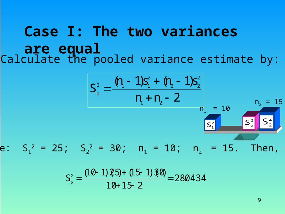
Case I: The two variances are equal

2nns)1n(s)1n(

S21

2

22

2

112

p

Example: S12 = 25; S2

2 = 30; n1 = 10; n2 = 15. Then,

04347.2821510

)30)(115()25)(110(S2

p

• Calculate the pooled variance estimate by:

2pS

n2 = 15n1 = 10

21S

22S

10

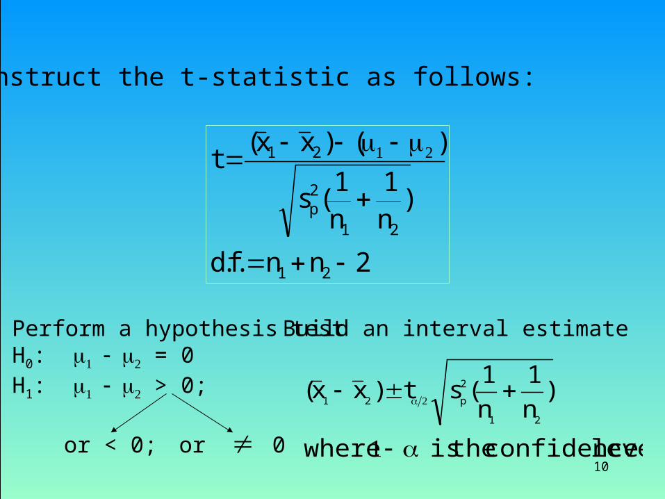
• Construct the t-statistic as follows:

2nn.f.d

)n1

n1

(s

)()xx(t

21

21

2p

21

• Perform a hypothesis test H0: = 0 H1: > 0;

or < 0; or 0

Build an interval estimate

level. confidence the is where

)n1

n1

(st)xx(21

2

p21

11

1)(

1)(

)/(d.f.

)(

)()(

2

2

222

1

21

21

22

221

21

2

22

1

21

21

nns

nns

nsns

ns

ns

xxt

Case II: The two variances are unequal

12

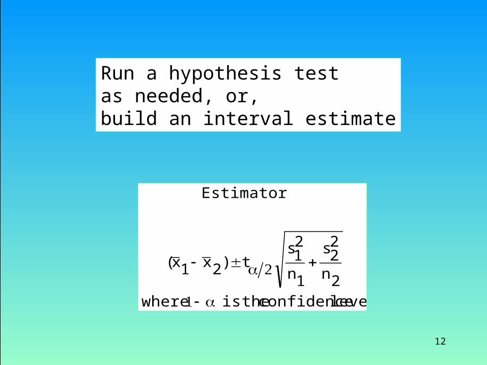
Run a hypothesis test as needed, or, build an interval estimate

level. confidence theis where

n

s

n

st)xx(

Estimator

2

22

1

21

21

13

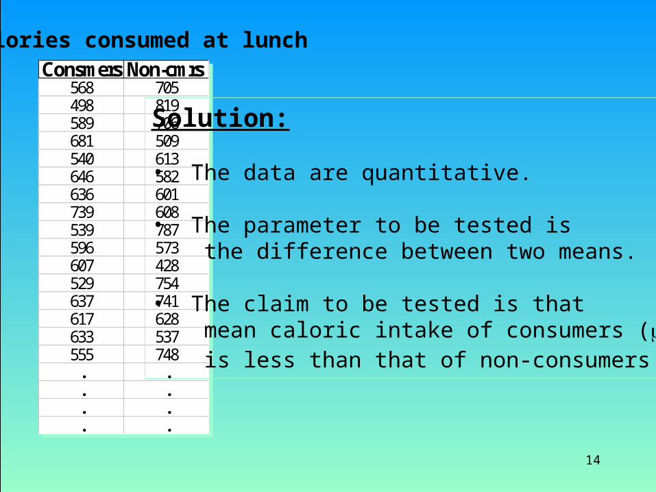
• Example 12.1– Do people who eat high-fiber cereal for

breakfast consume, on average, fewer calories for lunch than people who do not eat high-fiber cereal for breakfast?

– A sample of 150 people was randomly drawn. Each person was identified as a consumer or a non-consumer of high-fiber cereal.

– For each person the number of calories consumed at lunch was recorded.

14

Consmers Non-cmrs568 705498 819589 706681 509540 613646 582636 601739 608539 787596 573607 428529 754637 741617 628633 537555 748

. .

. .

. .

. .


. .

. .

. .

. .

Calories consumed at lunch

Solution: • The data are quantitative. • The parameter to be tested is the difference between two means. • The claim to be tested is that mean caloric intake of consumers (1) is less than that of non-consumers (2).

15

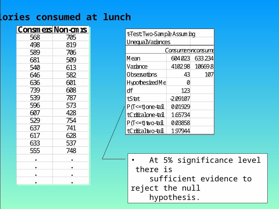
• Identifying the technique

–The hypotheses are:

H0: (1 - 2) = 0H1: (1 - 2) < 0

– To check the relationships between the variances, we use a computer output to find the samples’ standard deviations. We have S1 = 64.05, and S2

= 103.29. It appears that the variances are unequal.

– We run the t - test for unequal variances.

1 < 2)

16

Calories consumed at lunch

• At 5% significance level there is sufficient evidence to reject the null hypothesis.


. .

. .

. .

. .


. .

. .

. .

. .

t-Test: Two-Sample Assuming Unequal Variances

ConsumersNonconsumersMean 604.023 633.234Variance 4102.98 10669.8Observations 43 107Hypothesized Mean Difference0df 123t Stat -2.09107P(T<=t) one-tail 0.01929t Critical one-tail 1.65734P(T<=t) two-tail 0.03858t Critical two-tail 1.97944

17

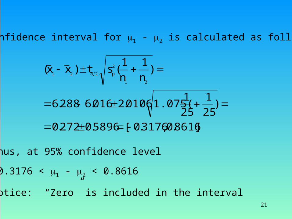
• Solving by hand– The interval estimator for the difference between two

means is

65.2721.29107

29.1034305.64

9796.1)239.63302.604(

)2n

22s

1n

21s

(2t)2x1x(

22

18

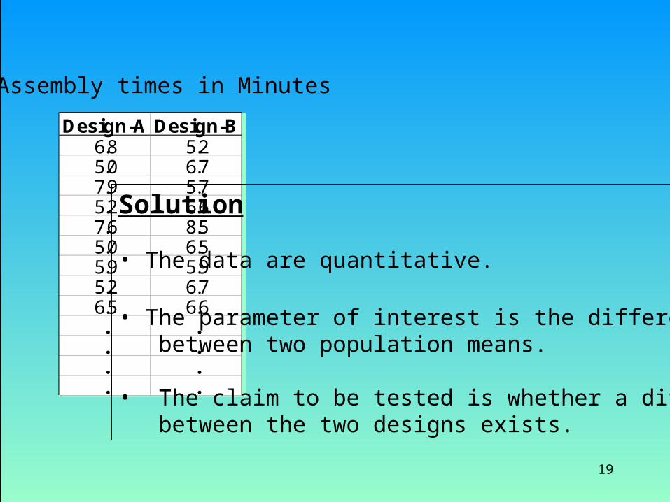
• Example 12.2

– Do job design (referring to worker movements) affect worker’s productivity?

– Two job designs are being considered for the production of a new computer desk.

– Two samples are randomly and independently selected• A sample of 25 workers assembled a desk using design A. • A sample of 25 workers assembled the desk using design B.• The assembly times were recorded

– Do the assembly times of the two designs differs?

19

Design-A Design-B6.8 5.25.0 6.77.9 5.75.2 6.67.6 8.55.0 6.55.9 5.95.2 6.76.5 6.6. .. .. .. .

Design-A Design-B6.8 5.25.0 6.77.9 5.75.2 6.67.6 8.55.0 6.55.9 5.95.2 6.76.5 6.6. .. .. .. .

Assembly times in Minutes

Solution

• The data are quantitative.

• The parameter of interest is the difference between two population means.

• The claim to be tested is whether a difference between the two designs exists.

20

Design-A Design-B6.8 5.25.0 6.77.9 5.75.2 6.67.6 8.55.0 6.55.9 5.95.2 6.76.5 6.6. .. .. .. .

Design-A Design-B6.8 5.25.0 6.77.9 5.75.2 6.67.6 8.55.0 6.55.9 5.95.2 6.76.5 6.6. .. .. .. .

t-Test: Two-Sample Assuming Equal Variances

Design-A Design-BMean 6.288 6.016Variance 0.847766667 1.3030667Observations 25 25Pooled Variance 1.075416667Hypothesized Mean Difference0df 48t Stat 0.927332603P(T<=t) one-tail 0.179196744t Critical one-tail 1.677224191P(T<=t) two-tail 0.358393488t Critical two-tail 2.01063358


Design-A Design-BMean 6.288 6.016Variance 0.847766667 1.3030667Observations 25 25Pooled Variance 1.075416667Hypothesized Mean Difference0df 48t Stat 0.927332603P(T<=t) one-tail 0.179196744t Critical one-tail 1.677224191P(T<=t) two-tail 0.358393488t Critical two-tail 2.01063358

The Excel printout

P-value of the one tail test

P-value of the two tail test

Degrees of freedomt - statistic

2

1S 2

2S2

pS

21

A 95% confidence interval for 1 - 2 is calculated as follows:

]8616.0,3176.0[5896.0272.0

)251

251

1.075(0106.2016.6288.6

)n1

n1

(st)xx(21

2

p21

Thus, at 95% confidence level

-0.3176 < 1 - 2 < 0.8616

Notice: “Zero” is included in the interval

22

Checking the required Conditions for the equal variances case (example 12.2)

The distributions are notbell shaped, but theyseem to be approximately normal. Since the techniqueis robust, we can be confidentabout the results.

0

2

4

6

8

10

12

5 5.8 6.6 7.4 8.2 More

Design A

01234567

4.2 5 5.8 6.6 7.4 More

Design B

23

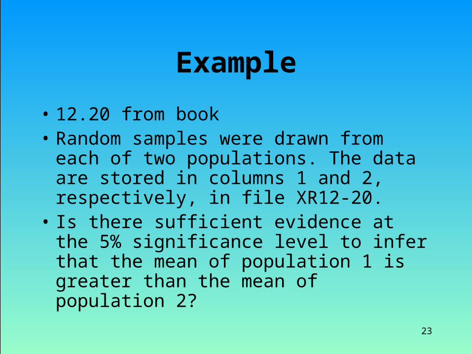
Example

• 12.20 from book• Random samples were drawn from each of two

populations. The data are stored in columns 1 and 2, respectively, in file XR12-20.

• Is there sufficient evidence at the 5% significance level to infer that the mean of population 1 is greater than the mean of population 2?

24

X1 X2

Mean 246.80 Mean 239.66Standard Error 2.88 Standard Error 0.94Median 247.00 Median 240.00Mode 280.00 Mode 240.00Standard Deviation 28.81 Standard Deviation 11.57Sample Variance 829.90 Sample Variance 133.81Kurtosis 0.34 Kurtosis 0.02Skewness -0.02 Skewness 0.02Range 162.00 Range 61.00Minimum 158.00 Minimum 213.00Maximum 320.00 Maximum 274.00Sum 24680.00 Sum 35949.00Count 100.00 Count 150.00Confidence Level(95.0%) 5.72 Confidence Level(95.0%) 1.87


X1 X2Mean 246.8 239.66Variance 829.89899 133.8097987Observations 100 150Hypothesized Mean Difference 0df 121t Stat 2.3551335P(T<=t) one-tail 0.0100626t Critical one-tail 1.657545P(T<=t) two-tail 0.0201252t Critical two-tail 1.9797653

25

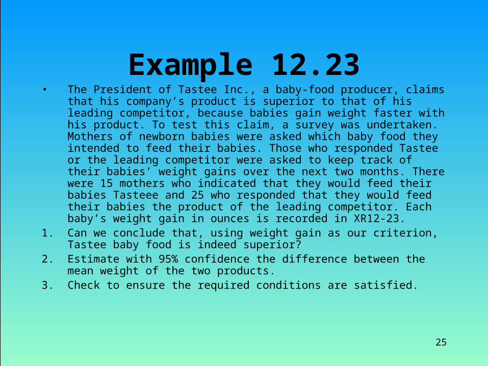
Example 12.23• The President of Tastee Inc., a baby-food producer, claims that his

company’s product is superior to that of his leading competitor, because babies gain weight faster with his product. To test this claim, a survey was undertaken. Mothers of newborn babies were asked which baby food they intended to feed their babies. Those who responded Tastee or the leading competitor were asked to keep track of their babies’ weight gains over the next two months. There were 15 mothers who indicated that they would feed their babies Tasteee and 25 who responded that they would feed their babies the product of the leading competitor. Each baby’s weight gain in ounces is recorded in XR12-23.

1. Can we conclude that, using weight gain as our criterion, Tastee baby food is indeed superior?

2. Estimate with 95% confidence the difference between the mean weight of the two products.

3. Check to ensure the required conditions are satisfied.

26

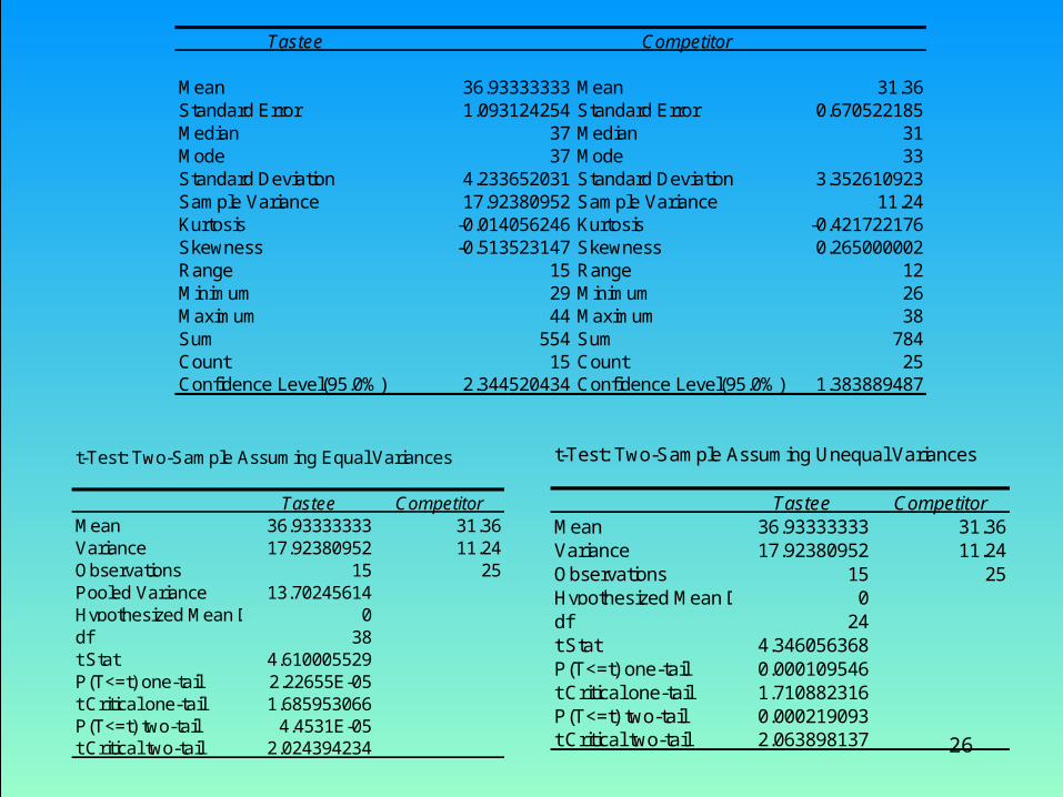
Tastee Competitor

Mean 36.93333333 Mean 31.36Standard Error 1.093124254 Standard Error 0.670522185Median 37 Median 31Mode 37 Mode 33Standard Deviation 4.233652031 Standard Deviation 3.352610923Sample Variance 17.92380952 Sample Variance 11.24Kurtosis -0.014056246 Kurtosis -0.421722176Skewness -0.513523147 Skewness 0.265000002Range 15 Range 12Minimum 29 Minimum 26Maximum 44 Maximum 38Sum 554 Sum 784Count 15 Count 25Confidence Level(95.0%) 2.344520434 Confidence Level(95.0%) 1.383889487


Tastee CompetitorMean 36.93333333 31.36Variance 17.92380952 11.24Observations 15 25Hypothesized Mean Difference 0df 24t Stat 4.346056368P(T<=t) one-tail 0.000109546t Critical one-tail 1.710882316P(T<=t) two-tail 0.000219093t Critical two-tail 2.063898137


Tastee CompetitorMean 36.93333333 31.36Variance 17.92380952 11.24Observations 15 25Pooled Variance 13.70245614Hypothesized Mean Difference 0df 38t Stat 4.610005529P(T<=t) one-tail 2.22655E-05t Critical one-tail 1.685953066P(T<=t) two-tail 4.4531E-05t Critical two-tail 2.024394234

27

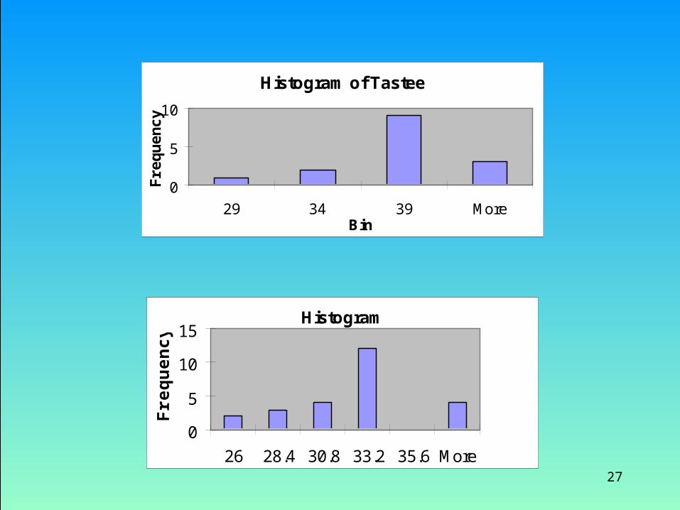
Histogram of Tastee

0

5

10

29 34 39 MoreBin

Fre

qu

en

cy

Histogram

0

5

10

15

26 28.4 30.8 33.2 35.6 More

Fre

qu

en

cy

Economics 173 Business Statistics Lecture 8 Fall, 2001 Professor J. Petry

Documents

Transcript of Economics 173 Business Statistics Lecture 8 Fall, 2001 Professor J. Petry