Economic Reforms and Regional Disparities in Economic and...

ECONOMIC REFORMS AND REGIONAL DISPARITIES IN ECONOMIC AND SOCIAL

DEVELOPMENT IN INDIA

(Report of a Research Project funded by the SER Division of the Planning Commission of the Government of India)

Dr. K.R.G.Nair Honorary Research Professor

Centre for Policy Research, Dharma Marg, Chanakya Puri, New Delhi –110021

August 2004

Table of Contents

Pages

Preface

1

Chapter 1 Introduction 2-7

Chapter 2 Pattern of Change over Time

8-20

Chapter 3 Explorations at Explanation 21-30

Chapter 4 Inter-state Disparities in industrial Development in India

31-58

Chapter 5 Main Findings / Conclusions 59-61

References 62-64

.

.

1

Preface

The project has been funded by the SER division of the Planning Commission of the Government of India. It has been carried out at the Centre for Policy Research, New Delhi. Work on the project formally began on the 15th of July 2003 and was to have been completed in a year’s time. The preliminary results of the project were widely circulated and also discussed at three seminars, two at the Centre for Policy Research on the 9th of February 2004 and on 28th of May 2004 and another at the University of Montenegro on the 11th of June 2004. A number of useful suggestions were received at these seminars and to the extent possible and necessary, these have been incorporated in the report. In order to do so, a month’s extension of time was sought for and was granted. As the Director of the project, I received considerable help from a large number of individuals and organisations in my work and I thank all of them for their whole-hearted co-operation in this regard. I would like to formally place on record my particular gratitude to the following: -

(1) Ms. Sreerupa, who was formally involved as a Research Associate in the project and helped me in a number of ways including the collection and analysis of data.

(2) The President and Faculty colleagues at the CPR (3) The library, computer centre and administrative staff of the CPR (4) The SER division of the Planning Commission of the Government of

India, and (5) The participants at the three seminars at which the preliminary results

of the project were discussed The usual disclaimers apply and the Project Director holds himself fully responsible for any errors or inconsistencies that have crept in to the Report. Centre for Policy Research New Delhi K.R.G.Nair 13th August 2004 Project Director

2

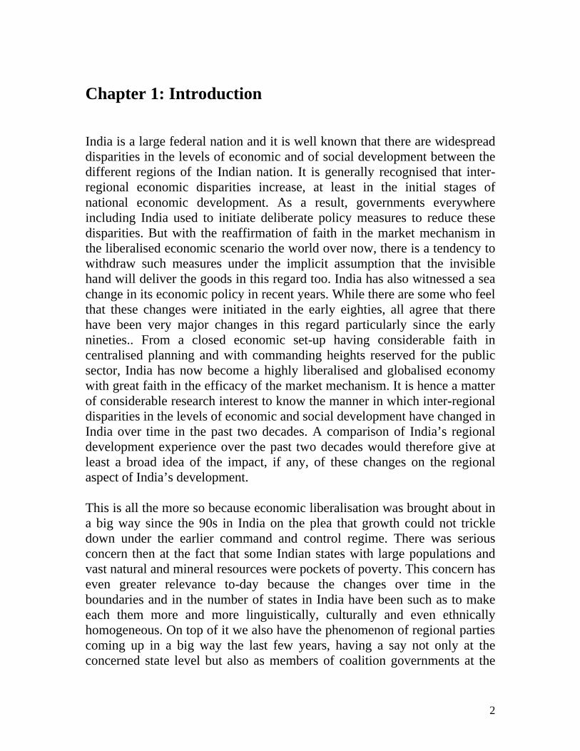
Chapter 1: Introduction

India is a large federal nation and it is well known that there are widespread disparities in the levels of economic and of social development between the different regions of the Indian nation. It is generally recognised that inter-regional economic disparities increase, at least in the initial stages of national economic development. As a result, governments everywhere including India used to initiate deliberate policy measures to reduce these disparities. But with the reaffirmation of faith in the market mechanism in the liberalised economic scenario the world over now, there is a tendency to withdraw such measures under the implicit assumption that the invisible hand will deliver the goods in this regard too. India has also witnessed a sea change in its economic policy in recent years. While there are some who feel that these changes were initiated in the early eighties, all agree that there have been very major changes in this regard particularly since the early nineties.. From a closed economic set-up having considerable faith in centralised planning and with commanding heights reserved for the public sector, India has now become a highly liberalised and globalised economy with great faith in the efficacy of the market mechanism. It is hence a matter of considerable research interest to know the manner in which inter-regional disparities in the levels of economic and social development have changed in India over time in the past two decades. A comparison of India’s regional development experience over the past two decades would therefore give at least a broad idea of the impact, if any, of these changes on the regional aspect of India’s development. This is all the more so because economic liberalisation was brought about in a big way since the 90s in India on the plea that growth could not trickle down under the earlier command and control regime. There was serious concern then at the fact that some Indian states with large populations and vast natural and mineral resources were pockets of poverty. This concern has even greater relevance to-day because the changes over time in the boundaries and in the number of states in India have been such as to make each them more and more linguistically, culturally and even ethnically homogeneous. On top of it we also have the phenomenon of regional parties coming up in a big way the last few years, having a say not only at the concerned state level but also as members of coalition governments at the

3

centre. In such a scenario, widespread inter-state disparities in levels of economic and social development can have serious economic, social and even political consequences, this being particularly so if these have persisted over long periods of time. A detaailed study examining the nature, extent, possible causes and manner of change of inter-state economic and social disparities in India and drawing broad inferences regarding regional policy in India would hence be of considerable relevance to policy-makers and planners in India, particularly since the period covered by the study includes a decade before the economic reforms and another afterwards. This is all the more so because at the time the study was undertaken, there was a real paucity of studies of this kind. A critical survey of studies related to Regional Economic Development in India by Nair (1993a) has clearly shown the paucity, till 1990, of studies of the type being attempted here. Earlier work mainly consisted of examining issues related to the choice of regions for anlaysis, estimation of indicators of regional well-being, regional impact studies and studies testing the validity of growth theories at the regional level. Barring few exceptions like the study by Nair (1982) dealing with the pre-80 period, these did not link regional development experience to government policies in this regard for regional development. The situation has remained more or less the same since the 90’s. There have of course been a number of meaningful studies about indicators of regional well being like the ones by Cassen(2002), Malhotra(1998) and the Planning Commission (2002). There have also been some attempts to find out the relationship between economic growth and poverty at the regional level like the one by Datt and Ravilion(2002). There were also some efforts at linking regional development experience to regional policy. One of these by Nair(1993 b) was a mere exploratory note and that too concerned with just one state – Orissa. The other was a much more detailed one by Kurian(2000) and dealt with the major Indian states, but it focused mostly on the period since the 80’s. There is no detailed study of inter-state regional experience in economic and social development in India examining the nature, extent and possible causes of disparities, the patterns of regional change and the inter-relationship between economic and social development at the regional level, linking all this up with changes in regional policy and covering both the pre and the post-reform periods

In view of all this, the states in India are hence taken as regions for the purpose of the study here. A question may arise as to whether it is appropriate to consider the states as regions for the purpose of this study

4

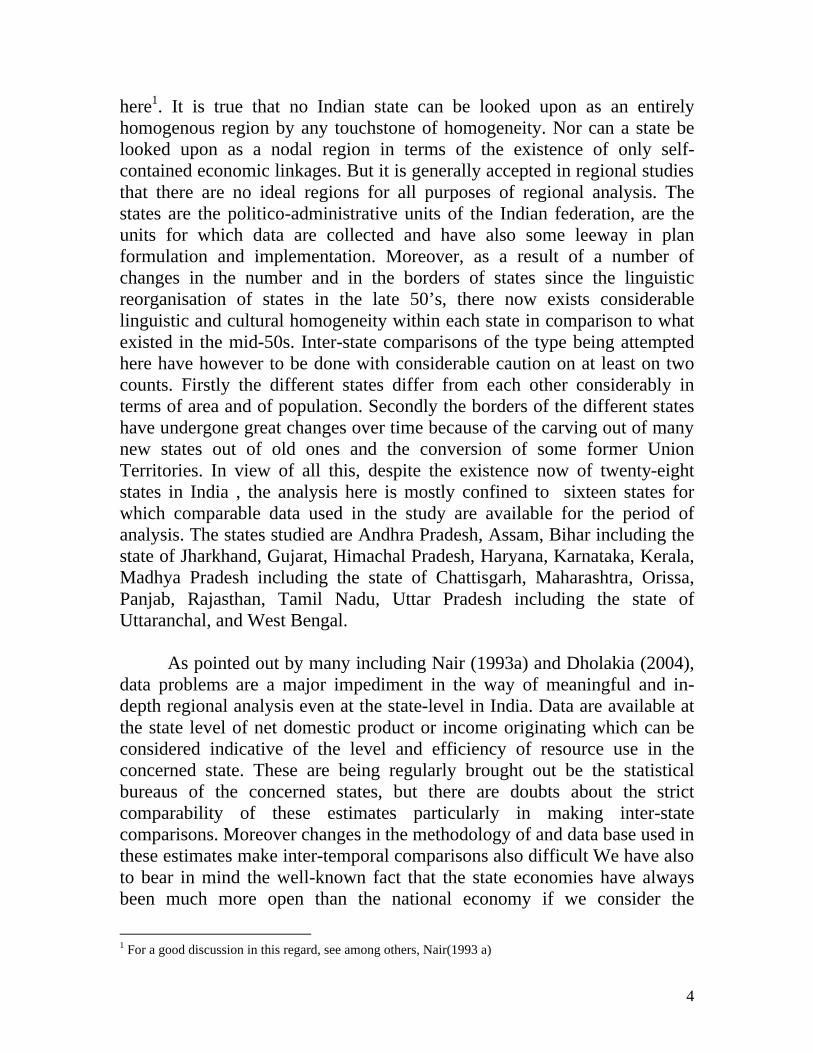
here1. It is true that no Indian state can be looked upon as an entirely homogenous region by any touchstone of homogeneity. Nor can a state be looked upon as a nodal region in terms of the existence of only self-contained economic linkages. But it is generally accepted in regional studies that there are no ideal regions for all purposes of regional analysis. The states are the politico-administrative units of the Indian federation, are the units for which data are collected and have also some leeway in plan formulation and implementation. Moreover, as a result of a number of changes in the number and in the borders of states since the linguistic reorganisation of states in the late 50’s, there now exists considerable linguistic and cultural homogeneity within each state in comparison to what existed in the mid-50s. Inter-state comparisons of the type being attempted here have however to be done with considerable caution on at least on two counts. Firstly the different states differ from each other considerably in terms of area and of population. Secondly the borders of the different states have undergone great changes over time because of the carving out of many new states out of old ones and the conversion of some former Union Territories. In view of all this, despite the existence now of twenty-eight states in India , the analysis here is mostly confined to sixteen states for which comparable data used in the study are available for the period of analysis. The states studied are Andhra Pradesh, Assam, Bihar including the state of Jharkhand, Gujarat, Himachal Pradesh, Haryana, Karnataka, Kerala, Madhya Pradesh including the state of Chattisgarh, Maharashtra, Orissa, Panjab, Rajasthan, Tamil Nadu, Uttar Pradesh including the state of Uttaranchal, and West Bengal.

As pointed out by many including Nair (1993a) and Dholakia (2004),

data problems are a major impediment in the way of meaningful and in-depth regional analysis even at the state-level in India. Data are available at the state level of net domestic product or income originating which can be considered indicative of the level and efficiency of resource use in the concerned state. These are being regularly brought out be the statistical bureaus of the concerned states, but there are doubts about the strict comparability of these estimates particularly in making inter-state comparisons. Moreover changes in the methodology of and data base used in these estimates make inter-temporal comparisons also difficult We have also to bear in mind the well-known fact that the state economies have always been much more open than the national economy if we consider the

1 For a good discussion in this regard, see among others, Nair(1993 a)

5

existence of considerable inter-state economic flows. In view of this, no serious analyst would consider the income originating in a state as indicative of the level of living of the people of the state concerned. In order to have a clearer understanding in this regard, it is necessary to examine other indicators like income originating or disposable personal income at the state level. But data regarding income accruing or personal income, available at the regional level in most countries of the world are conspicuous by their absence in India. However, in recent years, some serious efforts have been made to fill this important data gap. Planning Commission (2002) has brought out human development indicators at the state level for three points of time. Similarly the Economic and Political Weekly Research Foundation (EPWRF)(2002) has put together on a comparable basis data on state domestic product brought out by the different state statistical bureaus. The data from these two sources are mainly used for the purposes of analysis here.

Data limitations, shortness of the period studied and other constraints regarding the project have limited the nature of the work done here. No detailed and in-depth analysis of the relationship between regional policy and the nature and possible causes of inter-state disparities could be carried out. Further these also ruled out the application of advanced statistical and econometric techniques to analyse the data As pointed out by many including Hanna (1959), a usually accepted and simple way of carrying out regional analysis of this kind at the sub-national level is to compare the region concerned with the nation as a whole. This is done by working out region relatives, which give the position of the region concerned under the assumption that the value for the variable under study at the national level is 100. Subject to data limitations, comparisons between two single points of time are avoided and three-year averages are taken. The regions are then grouped into two, group one consisting of regions with values of relatives less than 100 and group two of regions with values of relative equal to or more than 100. However in the case of % people below the poverty line, states with state relative equal to or more than 100 are put in group one with the other states forming group two. The relative development experience of the different states is studied by looking at the manner in which these state relatives undergo change over time. In the case of all variables considered except the % people below the poverty line, when regional disparities lessen to lead to regional convergence, states of group one experience positive changes in the value of their relatives, while in the case of states of group two, state relatives experience negative changes over time with the exact

6

opposite happening when regional disparities increase to lead to regional divergence. In the case of the % people below the poverty line where the grouping has been done in a different manner, in the case of regional divergence, states of group one experience positive changes with the reverse happening to states of group two. Besides looking at the inter-temporal movement of states between the two groups in terms of the values of their respective state relatives, coefficients of correlation are worked out between the value of the state relative in the initial period and changes in this value over time. In order to decipher possible factors to explain inter-state disparities in HDI, in per capita net domestic product and in per capita value added in the different sectors analysed here, multiple linear regression equations are fitted to the data with state relative in HDI, per capita NSDP/ sectoral value added as the dependent variable. In the light of economic logic and earlier empirical indications, possible explanatory variables are chosen. The significance of the coefficients is tested at 5% level on the basis of the two-tailed t-statistic.

The study here is thus a preliminary exercise to enquire into the nature

and causes of change in inter-state disparities in the levels of economic and social development in India. This is done in the light of the prevalent views in this regard the world over. Attention is particularly focused on a comparison between India’s regional experience in the pre and in the post reform periods. The study analyses the manner in which inter-state disparities in economic development, as indicated by per capita net state domestic product (NSDP), have changed over time in India. It also carries out a similar exercise of other indicators of levels of living like consumer expenditure. % people below poverty line and human development index. An attempt is then made to get an idea as to which of the different hypotheses regarding the pattern of inter-regional change in the process of national economic development is valid in the case of India in the last two decades. The study also tries to explain not only inter-state disparities in HDI and in per capita NSDP but also such disparities in per capita value added in manufacturing, disaggregating the sector even further into registered and unregistered manufacturing. The study contains four more chapters besides this introductory one. Chapter two analyses the different prevalent hypotheses regarding the pattern of regional change in the process of national economic development and examines India’s regional experience in the light of these. Chapters three is an exploratory exercise in explaining inter-state disparities in per capita NSDP and HDI. Chapter four examines inter-state disparities in terms of per capita value added in manufacturing

7

industry attempting also to decipher the possible explanatory factors leading to these inter-state disparities. The last chapter brings together the main findings of the study attempting also to draw some policy inferences and suggesting some further lines of work.

8

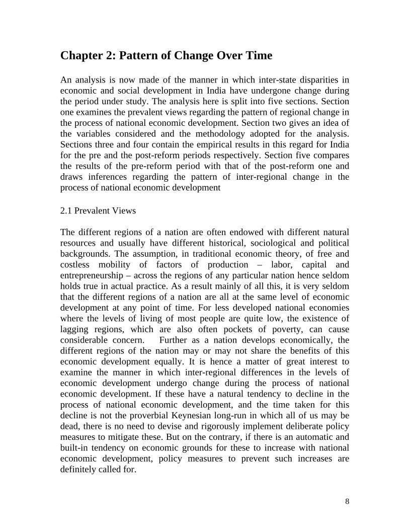
Chapter 2: Pattern of Change Over Time An analysis is now made of the manner in which inter-state disparities in economic and social development in India have undergone change during the period under study. The analysis here is split into five sections. Section one examines the prevalent views regarding the pattern of regional change in the process of national economic development. Section two gives an idea of the variables considered and the methodology adopted for the analysis. Sections three and four contain the empirical results in this regard for India for the pre and the post-reform periods respectively. Section five compares the results of the pre-reform period with that of the post-reform one and draws inferences regarding the pattern of inter-regional change in the process of national economic development 2.1 Prevalent Views The different regions of a nation are often endowed with different natural resources and usually have different historical, sociological and political backgrounds. The assumption, in traditional economic theory, of free and costless mobility of factors of production – labor, capital and entrepreneurship – across the regions of any particular nation hence seldom holds true in actual practice. As a result mainly of all this, it is very seldom that the different regions of a nation are all at the same level of economic development at any point of time. For less developed national economies where the levels of living of most people are quite low, the existence of lagging regions, which are also often pockets of poverty, can cause considerable concern. Further as a nation develops economically, the different regions of the nation may or may not share the benefits of this economic development equally. It is hence a matter of great interest to examine the manner in which inter-regional differences in the levels of economic development undergo change during the process of national economic development. If these have a natural tendency to decline in the process of national economic development, and the time taken for this decline is not the proverbial Keynesian long-run in which all of us may be dead, there is no need to devise and rigorously implement deliberate policy measures to mitigate these. But on the contrary, if there is an automatic and built-in tendency on economic grounds for these to increase with national economic development, policy measures to prevent such increases are definitely called for.

9

Considerable economic, and, since 1990s, econometric research has gone on to unravel the pattern of regional economic change in the process of national economic development. Myrdal (1956) and Hirschman (1961) have identified in detail the forces that operate to bring about these relative regional changes. While Myrdal (1956) refers to the forces of convergence and of divergence as spread and backwash effects, Hirschman(1961) describes these broadly as trickling-down and polarisation effects respectively. Scanning regional economic literature, one comes across at least three different hypotheses in this regard and these differ on the emphasis given to the relative importance over time of the forces of convergence and of divergence. One of these is the self-perpetuation hypothesis propounded by Hughes(1961) and found empirically valid by Booth(1964) for the USA. According to this view, the forces of divergence dominate over those of convergence and as a result, inter-regional differences in the levels of economic development keep on widening over time. A diametrically opposite view is the convergence hypothesis propounded and found empirically valid by Hanna(1959) and substantiated these days also with the Solovian logic that the rate of economic growth is inversely related to the level of per capita income and hence given identical technologies, preferences and rates of population growth, cotemporaneous differences in per capita incomes between any two regions will be transitory. Considerable evidence to support the hypothesis empirically has been provided by Hanna (1959), Perloff et al(1960) and more recently by Sala-i-Martin (1996) .The third hypothesis, which in a sense is a happy combination of these two diametrically opposite views is the concentration-cycle hypothesis propounded by Williamson(1965). The proponents of this view, point out that inter-regional economic differentials diverge initially to converge later on and thus trace out the famous Kuznetsian inverted U-shaped curve over time in the process of national economic development. Considerable empirical evidence in support of such a view emerged as a result of a detailed international study of regional development experiences by Williamson (1965). A new and valid point being stressed in this regard by many including Nair (1982) is that the pattern of regional change depends upon the indicator of development being considered, with different indicators showing different patterns of regional change.

10

2.2. Variables and Methodology Per capita NSDP at constant 1993-94 prices have been obtained from the data brought out by the EPWRF(2002). Average values of state relatives in per capita NSDP have been calculated for the years 1980-81 to 1982-83, 1987-88 to 1989-90, 1991-92 to 1993-94 and 1997-98 to 1999-2000. Three variables indicative of level of living have been considered. These are the human development index and the % people below the poverty line as brought out by Planning Commission (2002) and per capita private consumer expenditure for the years 1983, 1987-88, 1993-94 and 1998-99 calculated from the data contained in the reports of the 38th, 43rd, 50th and 55th rounds of the National sample Survey. State relatives have been calculated on the basis of each of these three variables. The pattern of change is examined by looking at the signs of change in these as well as by examining the coefficients of correlation between the values of the state relatives in the initial year/period and the % change in these values between the initial year/period and the terminal year/period have also been worked out. Such studies are carried out for the pre and the post-reform periods separately. The analysis is carried out to decipher the pattern of regional change with particular attention paid to see whether there are any differences in this regard between the pre and the post-reform periods in India 2.3 Pre-reform period

2.3.1 Per capita NSDP

11

Table 2.1 gives the state relatives of per capita NSDP at constant 1993-94 prices for the pre-reform period.

Table 2.1 State Relatives of Per Capita NSDP at constant (1993-94) prices for the Pre-reform period*.

State Relatives in

S.No State 1980-81 to 1982-83

1987-88 to 1989-90

% change

(1) (2) (3) (4) (5) 1 Bihar 62.33 59.71 -4.21 2 Orissa 71.40 70.83 -0.79 3 Uttar Pradesh 77.72 74.08 -4.69 4 Rajasthan 80.55 82.08 1.91 5 West Bengal 88.50 85.00 -3.95 6 Assam 89.81 78.02 -13.13 7 Andhra Pradesh 90.97 90.64 -0.37 8 Karnataka 93.26 94.39 1.21 9 Madhya Pradesh 93.92 83.27 -11.34 10 Tamil Nadu 100.16 102.41 2.25 11 Kerala 101.87 88.24 -13.38 12 Himachal Pradesh 105.87 101.52 -4.11 13 Gujarat 122.33 119.94 -1.96 14 Maharashtra 131.08 131.78 0.53 15 Haryana 140.33 143.96 2.59 16 Punjab 162.00 164.91 1.80

Note : *States are arranged in ascending order of the value of the state relative in the initial period, which refers to 1980-81 to 1982-83 . The terminal period refers to 1987-88 to 1989-90.

Source : Calculated from Economic and Political Weekly Research Foundation

(EPWRF) (2002): Domestic Product of States of India 1960-61 to 2000-01 The signs of the changes in the relatives given in column five of the table indicate that there are no definite tendencies toward regional convergence or divergence in the period. Of course one of the states- Kerala – which is in group two at the margin in the initial part of the pre-reform period goes down considerably to have a value lower than 100 in the terminal part of the pre-reform era. The largest as well as the smallest % change in the relative is in states of group with a value of relative equal to or greater than 100 in the initial period of the pre-reform era. Further though three of the seven states of group two undergo negative changes, six of the nine states of group one also undergo negative changes in the value of their

12

relatives. This gets further strengthened by the fact that the coefficient of correlation between the value of the state relative in the initial period of the pre-reform era and its % change during the period is only 0.31 which is not statistically significant.

2.3.2 Regional levels of Living

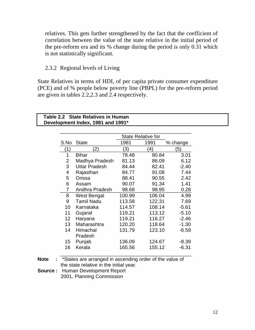
State Relatives in terms of HDI, of per capita private consumer expenditure (PCE) and of % people below poverty line (PBPL) for the pre-reform period are given in tables 2.2,2.3 and 2.4 respectively.

Table 2.2 State Relatives in Human Development Index, 1981 and 1991*

State Relative for S.No State 1981 1991 % change (1) (2) (3) (4) (5) 1 Bihar 78.48 80.84 3.01 2 Madhya Pradesh 81.13 86.09 6.12 3 Uttar Pradesh 84.44 82.41 -2.40 4 Rajasthan 84.77 91.08 7.44 5 Orissa 88.41 90.55 2.42 6 Assam 90.07 91.34 1.41 7 Andhra Pradesh 98.68 98.95 0.28 8 West Bengal 100.99 106.04 4.99 9 Tamil Nadu 113.58 122.31 7.69 10 Karnataka 114.57 108.14 -5.61 11 Gujarat 119.21 113.12 -5.10 12 Haryana 119.21 116.27 -2.46 13 Maharashtra 120.20 118.64 -1.30 14 Himachal

Pradesh 131.79 123.10 -6.59

15 Punjab 136.09 124.67 -8.39 16 Kerala 165.56 155.12 -6.31

Note : *States are arranged in ascending order of the value of the state relative in the initial year.

Source : Human Development Report 2001, Planning Commission

13

Table 2.3 State Relatives of Per Capita Private Consumer Expenditure in the Pre-reform period *

State Relative for S.No State 1983 1987-88 % change (1) (2) (3) (4) (5) 1 Bihar 79.54 78.76 -0.98 2 Orissa 83.16 77.36 -6.98 3 Uttar Pradesh 88.27 89.24 1.10 4 Madhya

Pradesh 89.20 90.12 1.03

5 Assam 94.20 91.63 -2.73 6 West Bengal 97.52 97.53 0.00 7 Andhra Pradesh 100.91 98.49 -2.40 8 Tamil Nadu 103.44 102.66 -0.75 9 Karnataka 106.14 94.59 -10.88 10 Gujarat 106.76 103.78 -2.79 11 Rajasthan 107.49 105.42 -1.93 12 Maharashtra 110.74 113.75 2.72 13 Kerala 121.58 124.32 2.25 14 Haryana 125.49 123.15 -1.87 15 Himachal

Pradesh 126.68 121.85 -3.81

16 Punjab 139.26 138.56 -0.51

Note : *States are arranged in ascending order of the value of the state relative in the initial year, which refers to 1983 on the basis of the 38rd Round of the NSS. The terminal year refers to 1987-88 corresponding to the 43rd Round of the NSS.

Source : Human Development Report 2001, Planning Commission.

43rd Round of the NSS

14

Table 2.4 State Relatives of Percentage of Population below Poverty line in the Pre-reform period *

State Relative for S.No State 1983 1987-88 %

change

(1) (2) (3) (4) (5) 1 Orissa 146.79 143.03 -2.56 2 Bihar 139.88 134.15 -4.10 3 West Bengal 123.31 115.08 -6.68 4 Tamil Nadu 116.14 111.66 -3.86 5 Madhya

Pradesh 111.92 110.83 -0.97

6 Uttar Pradesh 105.82 106.69 0.82 7 Maharashtra 97.66 103.99 6.48 8 Assam 90.98 93.18 2.41 9 Kerala 90.87 81.81 -9.98 10 Karnataka 85.97 96.58 12.34 11 Rajasthan 77.47 90.45 16.75 12 Gujarat 73.72 81.16 10.10 13 Andhra Pradesh 65.00 66.55 2.39 14 Haryana 48.04 42.82 -10.87 15 Himachal

Pradesh 36.87 39.76 7.83

16 Punjab 36.38 33.97 -6.62

Note : *States are arranged in descending order of the value of the state relative in the initial year, which refers to 1983 on the basis of the 38rd Round of the NSS. The terminal year refers to 1987-88 corresponding to the 43rd Round of the NSS.


15

The tables indicate that there has on the whole been a tendency of convergence if we look at the signs of the % change in the value of the relatives between the initial and the terminal years of the pre-reform period. In the case of HDI while seven of the nine states of group two undergo negative changes, six of the seven states of group one undergo positive changes in the value of their relatives. The coefficient of correlation between the value of the relative in the initial year and the % change in it is negative. Actually the value is as high as - 0.70 and is significant. As regards state relatives in per capita private consumer expenditure, the signs of change in these do indicate a tendency towards convergence. In fact two of the seven states of group two – Andhra Pradesh and Karnataka shift from group two to group one during the period. It is also true that seven of the ten states of group two experience a decline in the value of their relatives. But only three of the six states of group one undergo positive changes in this regard. As a result, no definite inference can be drawn in this regard particularly since the coefficient of correlation between the value of the state relative in the initial year and the % change in it during the period 0.09 and is not significant. The changes in the state relatives in % people below the poverty line also give some indications of regional convergence in poverty reduction2. The relative positions of five of the six states of group one undergo declines while six of the ten states of group two experience increase in their relative positions on this count with the state of Maharashtra changing during the period from group two to group one as a result. These changes are however not reflected in the coefficient of correlation between state relatives in the initial year and the % change in it during the period. The value of this coefficient is of course negative but is only –0.18 and is not significant

2.4 The post-reform period

2.4.1 Per Capita NSDP

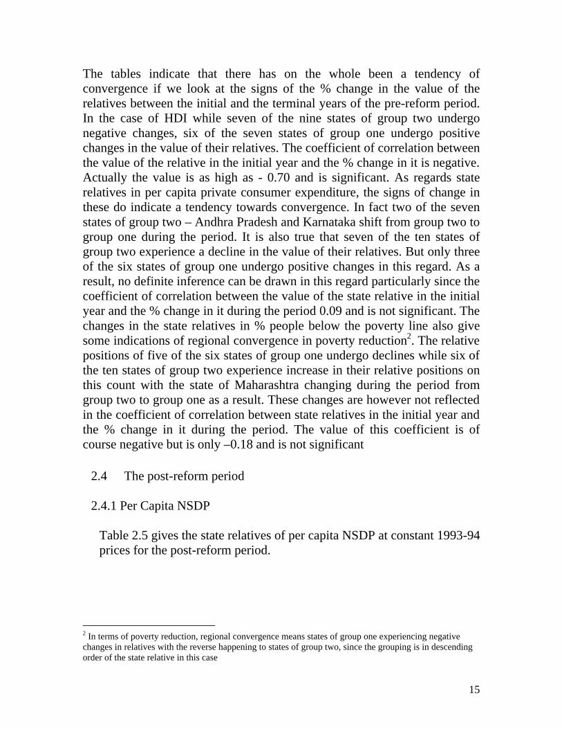
Table 2.5 gives the state relatives of per capita NSDP at constant 1993-94 prices for the post-reform period.

2 In terms of poverty reduction, regional convergence means states of group one experiencing negative changes in relatives with the reverse happening to states of group two, since the grouping is in descending order of the state relative in this case

16

Table 2.5 State Relatives of Per Capita NSDP at constant (1993-94)

prices for the Post-reform period*.

State

Relatives in

S.No State 1991-92 to 1993-94

1997-98 to 1999-2000

% change

(1) (2) (3) (4) (5) 1 Bihar 51.20 41.93 -18.11 2 Orissa 62.23 53.65 -13.78 3 Uttar Pradesh 69.30 56.78 -18.07 4 Assam 74.84 59.55 -20.42 5 Madhya Pradesh 81.33 75.85 -6.74 6 Rajasthan 85.01 89.03 4.73 7 West Bengal 86.34 90.58 4.92 8 Andhra Pradesh 94.01 91.50 -2.67 9 Kerala 97.19 98.50 1.34 10 Karnataka 100.14 105.88 5.73 11 Himachal Pradesh 101.52 103.29 1.74 12 Tamil Nadu 111.64 120.87 8.27 13 Gujarat 123.63 134.78 9.02 14 Haryana 146.21 133.95 -8.38 15 Maharashtra 147.12 146.20 -0.63 16 Punjab 164.06 146.78 -10.54

Note: *States are arranged in ascending order of the value of the state relative in the initial period, which refers to 1991-92 to 1993-94 . The terminal period refers to 1997-98 to 1999-2000.

Source: Calculated from Economic and Political Weekly Research Foundation

(EPWRF) (2002): Domestic Product of States of India 1960-61 to 2000-01

The signs of the changes in the relatives given in column five of the table indicate that there are definite tendencies towards regional divergence in the post-reform period. Six of the nine states, of group one, experience negative changes. The largest negative change is in Assam What seems even more striking is the fact that the second and third largest negative changes have taken place in the least developed states of India – Bihar and Uttar Pradesh. Four of the six states of group two undergo positive changes in their relatives and the largest positive change has in fact taken

17

place in one of the most developed states of India - Gujarat. All this is reflected in the fact that the correlation coefficient between the state relative in the initial year and its % change during the post-reform period is positive and has a value of 0.35 which is higher than the one in the pre-reform period. Nothing very definite can however be said in this regard on the basis of this value because it is not significant.

2.4.2 Regional levels of Living

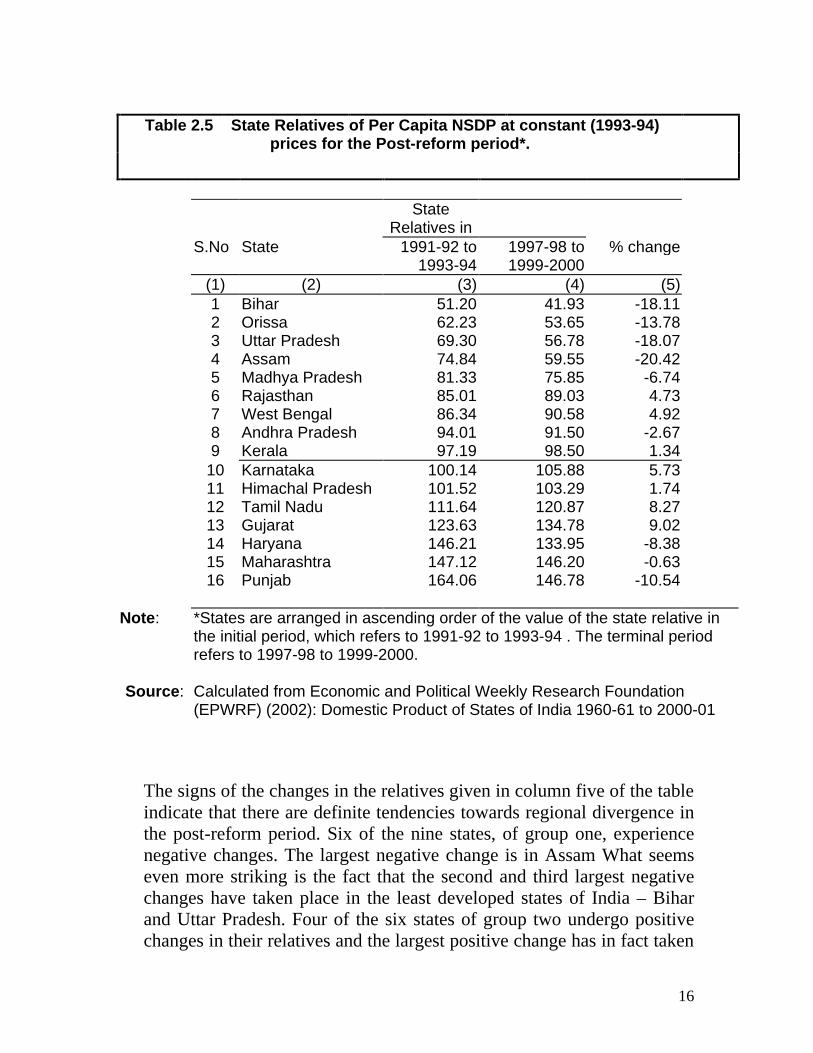
State Relatives in terms of HDI, of per capita private consumer expenditure and of % people below poverty line for the pre-reform period are given in tables 2.6,2.7 and 2.8 respectively. Table 2.6 State Relatives in Human Development Index,

1991 and 2001*

State

Relative for

S.no State 1991 2001 % change (1) (2) (3) (4) (5) 1 Bihar 80.84 77.75 -3.82 2 Uttar Pradesh 82.41 82.20 -0.26 3 Madhya Pradesh 86.09 83.47 -3.04 4 Orissa 90.55 85.59 -5.48 5 Rajasthan 91.08 89.83 -1.37 6 Assam 91.34 81.78 -10.47 7 Andhra Pradesh 98.95 88.14 -10.93 8 West Bengal 106.04 100.00 -5.69 9 Karnataka 108.14 101.27 -6.35 10 Gujarat 113.12 101.48 -10.29 11 Haryana 116.27 107.84 -7.25 12 Maharashtra 118.64 110.81 -6.60 13 Tamil Nadu 122.31 112.50 -8.02 14 Punjab 124.67 113.77 -8.74 15 Kerala 155.12 135.17 -12.86

Note : *States are arranged in ascending order of the value of the state relative in the initial year.

Source : Human Development Report 2001, Planning Commission

18

Table 2.7 State Relatives of Per Capita Private Consumer

Expenditure in the Post-reform period *

State

Relative for

S.no State 1993-94 1999-2000 % change (1) (2) (3) (4) (5) 1 Bihar 72.15 70.59 -2.16 2 Orissa 74.94 70.00 -6.59 3 Assam 85.45 80.11 -6.25 4 Madhya Pradesh 88.31 81.04 -8.24 5 Uttar Pradesh 90.69 87.48 -3.54 6 Karnataka 97.04 108.09 11.39 7 Andhra Pradesh 98.20 93.16 -5.14 8 West Bengal 101.58 96.73 -4.77 9 Tamil Nadu 104.91 115.29 9.89 10 Rajasthan 105.61 103.42 -2.08 11 Gujarat 108.74 114.77 5.54 12 Maharashtra 113.21 118.01 4.24 13 Himachal Pradesh 117.69 124.85 6.08 14 Haryana 124.22 129.94 4.60 15 Kerala 127.70 138.20 8.23 16 Punjab 139.13 134.03 -3.67

Note: *States are arranged in ascending order of the value of the state relative in the initial year, which refers to 1993-94 on the basis of the 50th Round of the NSS. The terminal year refers to 1999-2000 corresponding to the 55th Round of the NSS.


19

Table 2.8 State Relatives of Percentage of Population below Poverty line in the Post-reform period *

State Relative

for

S.no

State 1993-94 1999-2000 % change

(1) (2) (3) (4) (5) 1 Bihar 152.79 163.22 6.82 2 Orissa 135.00 180.65 33.81 3 Madhya Pradesh 118.21 143.41 21.32 4 Assam 113.59 138.28 21.73 5 Uttar Pradesh 113.57 119.35 5.09 6 Maharashtra 102.47 95.86 -6.45 7 West Bengal 99.14 103.52 4.42 8 Tamil Nadu 97.39 80.92 -16.91 9 Karnataka 92.19 76.78 -16.71 10 Himachal Pradesh 79.07 29.23 -63.03 11 Rajasthan 76.20 58.54 -23.17 12 Kerala 70.70 48.74 -31.06 13 Haryana 69.64 33.49 -51.92 14 Gujarat 67.31 53.91 -19.91 15 Andhra Pradesh 61.69 60.42 -2.06 16 Punjab 32.72 23.60 -27.87

Note : *States are arranged in descending order of the value of the state relative in the initial year, which refers to 1993-94 on the basis of the 50th Round of the NSS. The terminal year refers to 1999-2000 corresponding to the 55th Round of the NSS.


The tables indicate that while the converging tendency of HDI continues in

the post-reform period also, there are definite tendencies of inter-regional divergence if we consider per capita private consumer expenditure and the % people below the poverty line Nothing can be said in this regard on the basis of the signs of change of relatives of HDI because they are all negativei3.

3 This could be because a number of states heave been left out

20

The coefficient of correlation between the value of the relative in the initial year and the % change in it during the period is negative and significant having a value of -0.69, which is almost the same as in the pre-reform period. There are however indications of regional divergence if we consider per capita private consumer expenditure. Six of the seven states of group one undergo negative changes in the value of their relatives and six of the nine states of group two undergo positive changes in their relative positions in the post-reform period. Actually the correlation coefficient between the value of the relative in the initial period and the % change in it over time is positive and high at 0.46, though not statistically significant. As regards the % people below the poverty line, there has on the whole been a tendency of divergence if we look at the signs of the % change in the value of the relatives between the initial and the terminal years of the post-reform period. Five of the six states of group one undergo positive changes with Orissa – one of the least developed states of India - experiencing the largest positive increase. Only one of the ten states of group two undergoes a positive change in this regard. The coefficient of correlation between the initial value of the relative and its % change is positive in the post-reform period in contrast with the pre-reform one. The value however is only 0.21 and is not statistically significant4.

2.5 Main Findings The analysis here has revealed that the pattern of regional change in the pre and post-reform periods have been somewhat different. As regards per capita NSDP, while there are no definite indications of either divergence or convergence at the regional level in the pre-reform era considered here, the evidence here points towards divergence in the post-reform period. The more worrisome aspect is that if we consider indicators of levels of living, there are signs of inter-state convergence in the pre-reform period, while there are definite indications of inter-state divergence in the post-reform one. Another finding also stands out quite clearly. Irrespective of whether we are concerned with the pre or post-reform era, the indications here are that the pattern of regional change depends upon the variable considered as suggested in the multi-pattern hypothesis of regional change in the process of national economic development

4 There have been criticisms of the new reference period adopted for the 55th round of the NSS and if we use data adjusted for this difference by Kijima and Lanjouw(2004), the coefficient is 0.68 and is significant.

21

Chapter 3: Explorations at Explanation 3.1 introduction This chapter contains an exploratory effort to examine the possible reasons for inter-state disparities in India. Since infrastructure is usually considered the key to economic and social development, it is necessary to examine the relative position of a state in terms of infrastructural development as one of the factors influencing its relative position in terms of both per capita NSDP and in terms of overall human development. The Centre for Monitoring the Indian Economy has brought out indices of infrastructural development for the years 1981 and 1991. These are used to get state relatives (RIID) in this regard for the initial and terminal years of the pre-reform period. The indices of infrastructural development as brought out by the reports of the tenth and the eleventh Finance Commisions in India have been used to get RIID for the initial and the terminal years of the post-reform period. Another crucial factor, which is somehow not usually considered in this regard is the extent of poverty as indicated by the % people below the poverty line. What is generally taken for granted is that economic growth is accompanied by reductions in the extent of poverty. There is less recognition of the simple fact that the less the extent of poverty, the greater will be the extent of the market, the more will be the productivity of labour and hence the greater the level of economic development and also the overall level of human development. The study here hence considers the relative position of the state in terms of the % people below the poverty line (RPBPL) as one of the other important factors affecting the relative position of the state in terms of both per capita NSDP as well as in terms of HDI. A number of earlier critical studies of regional policy in India including the one by Nair (1982) had pointed out that the neglect of agriculture has been responsible for increasing regional disparities in India. This resulted in special efforts being made to extend the green revolution to the rice-growing and less developed eastern regions of India since the eighties. In view of this, the analysis here also goes on to examine the manner in which the relative positions of the different states of India have changed over time in terms of per capita value added in agriculture and allied sectors (RVAA). There is also considerable controversy these days about the development in India in the pre-reform period being mere creation of jobs without much economic growth and post-reform development being one of jobless growth. The chapter cxamines the validity of this argument at the state level in India on the basis of data on

22

employment brought out in the 38th, 50th and 55th rounds of the NSSO on Employment and Unemployment situation in India and the data on NSDP brought out by the EPWRF(2002). The analysis is carried out in six parts in addition to this introductory one. Part two contains an exercise to explain the state relatives in terms of HDI by means of state relatives in terms of infrastructural development and of per cent people below the poverty line. Part three contains such an exercise for state relatives of per capita NSDP. Part four examines the way in which relatives in terms of the index of infrastructural development have changed in the pre and post-reform periods. Part five carries out such a study about relatives in terms of per capita value added in agriculture and allied activities. Part six examines the rate of growth of NSDP and of employment in the pre and post-reform periods in India. Part seven brings together the main findings of this chapter. 3.2 State Relatives in HDI Table 3,1 gives the regression equations with the state relative in per capita HDI as the dependent variable and RIID and RPBPL as possible explanatory variables for different points of time

Table 3.1 Regression Equations with State Relative in HDI as the dependent variable *

Sl.No. Period Equation R squared

R bar squared

1 Pre-reform beginning RHDI = 60.04 + 0.46 RIID - 0.06 RPBPL (24.33) (0.12) (0.15) 0.66 0.6 [2.47] [3.90] [-0.42] 2 Pre-reform end RHDI = 47.29 + 0.04 RPBPL + 0.49 RIID (26.23) (0.15) (0.13) 0.65 0.59 [1.80] [0.26] [3.75] 3 Post reform end RHDI = 61.20 + 0.36 RIID - 0.04 RPBPL (14.72 ) (0.09) (0.06) 0.78 0.75 [4.16] [4.14] [-0.57] 4 Post reform end with RHDI = 59.38 + 0.37 RIID - 0.03 RPBPL Yoko Kijima and (16.58) (0.09) (-0.08) 0.78 0.74 Peter Lanjouw estimates [3.58] [4.25] [-0.37] of PBPL

Note :

1. The values of variables are from other tables elsewhere in the report.In this and subsequent tables, variables in bold font have

23

coefficients which are significant, and figures in round and square brackets give standard errors and t-values respectively.

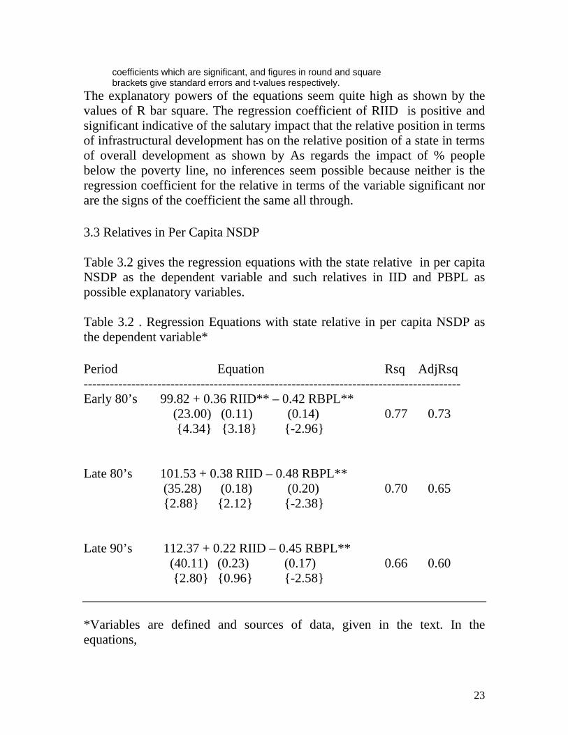
The explanatory powers of the equations seem quite high as shown by the values of R bar square. The regression coefficient of RIID is positive and significant indicative of the salutary impact that the relative position in terms of infrastructural development has on the relative position of a state in terms of overall development as shown by As regards the impact of % people below the poverty line, no inferences seem possible because neither is the regression coefficient for the relative in terms of the variable significant nor are the signs of the coefficient the same all through. 3.3 Relatives in Per Capita NSDP Table 3.2 gives the regression equations with the state relative in per capita NSDP as the dependent variable and such relatives in IID and PBPL as possible explanatory variables. Table 3.2 . Regression Equations with state relative in per capita NSDP as the dependent variable* Period Equation Rsq AdjRsq --------------------------------------------------------------------------------------- Early 80’s 99.82 + 0.36 RIID** – 0.42 RBPL** (23.00) (0.11) (0.14) 0.77 0.73 {4.34} {3.18} {-2.96} Late 80’s 101.53 + 0.38 RIID – 0.48 RBPL** (35.28) (0.18) (0.20) 0.70 0.65 {2.88} {2.12} {-2.38} Late 90’s 112.37 + 0.22 RIID – 0.45 RBPL** (40.11) (0.23) (0.17) 0.66 0.60 {2.80} {0.96} {-2.58} *Variables are defined and sources of data, given in the text. In the equations,

24

The high value for R bar square indicates that the explanatory power of the equation is high, though this seems to go down over time. But the interesting thing is that the coefficient for RPBPL is significant in all the three periods considered. The sign of the coefficient is negative indicating that the less the relative poverty, the higher the relative position in per capita NSDP. As regards RIID, while the signs of the coefficients are along expected lines it is significant only in one of the three periods considered. 3.4 State Relatives in IID Tables 3.3 and 3.4 give the values of RIID for the pre-reform and the post-reform periods respectively. The tables also contain the changes in these in each period.

Table 3.3 State Relatives in the Index of Infrastructural Development,1980-81 & 1990-91*

State Relatives in S. No State 1980-81 1990-91 % change (1) (2) (3) (4) (5) 1 Madhya Pradesh 62.1 69.7 12.2 2 Rajasthan 74.4 79.2 6.5 3 Assam 77.7 84 8.1 4 Orissa 81.5 93.5 14.7 5 Bihar 83.5 79.7 -4.6 6 Himachal Pradesh 83.5 95.9 14.9 7 Karnataka 94.8 96.4 1.7 8 Uttar Pradesh 97.7 103.6 6.0 9 Andhra Pradesh 98.1 97 -1.1 10 West Bengal 110.6 93.8 -15.2 11 Maharashtra 120.1 111.5 -7.2 12 Gujarat 123 122 -0.8 13 Haryana 145.5 139.7 -4.0 14 Kerala 158.1 157.4 -0.4 15 Tamil Nadu 158.6 145.5 -8.3 16 Punjab 207.3 192.6 -7.1

Note : *States are arranged in ascending order of the value of the state relative in the initial year, which refers to 1980-81.

Source : CMIE

25

Table 3.4 State Relatives in the Index of Infrastructural Development, in early and late 90's.*

State Relatives for S.No State Early

90's Late 90's % change

(1) (2) (3) (4) (5) 1 Madhya Pradesh 65.9 75.8 15.0 2 Rajasthan 70.5 75.9 7.7 3 Orissa 74.5 81.0 8.8 4 Himachal Pradesh 80.9 95.0 17.4 5 Assam 81.9 77.7 -5.2 6 Bihar 92.0 81.3 -11.6 7 Andhra Pradesh 99.2 103.3 4.1 8 Karnataka 101.2 104.9 3.6 9 Uttar Pradesh 111.8 101.2 -9.5 10 Maharashtra 121.7 112.8 -7.3 11 Gujarat 123.0 124.3 1.1 12 West Bengal 131.7 111.3 -15.5 13 Tamil Nadu 149.9 149.1 -0.5 14 Haryana 158.9 137.5 -13.4 15 Kerala 205.4 178.7 -13.0 16 Punjab 219.2 187.6 -14.4

Note : *States are arranged in ascending order of the value of the state relative in the initial period, which refers to early 90's.Infact the initial and terminal periods are 1990-95 & the year 1999 respectively.

Source : Tenth & Eleventh Finance Commission Reports It is clear from table 3.3 that inter-state disparities in IID seem to be in the convergent phase. In fact seven of the nine states of group one undergo positive changes in RIID while all the seven states of group two experience negative changes in this regard in the pre-reform era. Actually the second largest increase in this regard occurred in Orissa one of the least developed states of India The largest decline in this regard occurred in West Bengal making the state move from group one to group two during the period. Panjab and Maharashtra, which are developed states, experience the third and fourth largest declines on this count. All this is substantiated by the fact that there is a negative and significant correlation of - 0.62 between RIID in the initial year and its % change during the pre-reform era.

26

A similar picture emerges for the post-reform era from table 3.4. Substantial increases take place in this regard in less developed states like Madhya Pradesh - ranking number two in this regard - Orissa and Rajasthan. Five of the seven states of group one undergo positive changes and seven of the nine states of group two experience negative ones in the post-reform era. Andhra Pradesh actually shifts from group one to group two as a result of positive changes of this kind. The evidence in this regard gets further corroborated by the fact that the coefficient of correlation between RIID and the % change in it during the post-reform era is both negative and significant. Its value is - 0.70, a shade higher than the corresponding value in the pre-reform period. 3.5 State Relatives in VAA Tables 3,5 and 3.6 give the values of RVAA in the pre and the post-reform periods respectively. The tables also give the values of the % change in RVAA in each of the periods Table 3.5 State Relatives of Per Capita Value Added in Agriculture at 1980-81 Prices

for the Pre-reform period*. State Relatives for S.No State 1980-81 to

1982-83 1989-90 to

1991-92 % change

(1) (2) (3) (4) (5) 1 Tamil Nadu 61.78 72.47 17.31 2 Bihar 66.17 62.55 -5.47 3 West Bengal 78.33 96.19 22.80 4 Kerala 86.64 86.57 -0.07 5 Assam 95.21 87.83 -7.76 6 Rajasthan 98.31 112.75 14.69 7 Uttar Pradesh 101.80 96.05 -5.65 8 Maharashtra 102.25 102.38 0.13 9 Orissa 102.28 89.77 -12.23 10 Andhra Pradesh 106.49 97.70 -8.26 11 Karnataka 109.24 105.60 -3.33 12 Madhya Pradesh 109.37 96.38 -11.87 13 Gujarat 123.09 94.58 -23.16 14 Himachal Pradesh 128.21 122.31 -4.60 15 Haryana 192.40 212.52 10.46 16 Punjab 215.66 255.82 18.62

Note : *States are arranged in ascending order of the value of the state relative in the initial period, which refers to 1980-81 to 1982-83 . The terminal period refers to 1987-88 to 1989-90. Agriculture covers Agriculture, Forestry and Logging and Fishing.

Source : Calculated from Economic and Political Weekly Research Foundation (EPWRF) (2002): Domestic Product of States of India 1960-61 to 2000-01

27

Table 3.6 State Relatives of Per Capita Value Added in Agriculture at 1993-94

Prices for the Post-reform period*.

State Relatives for S.No State 1993-94 to

1995-96 1998-99 to 2000-2001

% change

(1) (2) (3) (4) (5) 1 Bihar 60.53 54.58 -9.83 2 Uttar Pradesh 79.85 75.97 -4.87 3 Orissa 81.60 70.87 -13.14 4 Tamil Nadu 89.66 87.76 -2.12 5 Assam 91.64 85.57 -6.62 6 West Bengal 93.93 96.05 2.26 7 Rajasthan 94.87 92.81 -2.18 8 Maharashtra 95.14 84.85 -10.81 9 Madhya Pradesh 100.36 92.74 -7.59 10 Andhra Pradesh 102.20 104.52 2.26 11 Kerala 102.29 96.17 -5.98 12 Himachal Pradesh 106.11 95.41 -10.08 13 Gujarat 109.40 92.70 -15.27 14 Karnataka 111.07 126.52 13.91 15 Haryana 183.11 171.28 -6.46 16 Punjab 233.94 224.74 -3.93

Note: *States are arranged in ascending order of the value of the state relative in the initial period, which refers to 1993-94 to 1995-96 . The terminal period refers to 1998-1999 to 2000-2001. Agriculture covers Agriculture, Forestry and Logging and Fishing

Source : Calculated from Economic and Political Weekly Research Foundation (EPWRF) (2002): Domestic Product of States of India 1960-61 to 2000-01

There are some indications of inter-state convergence in the pre-reform period. This is brought out if we examine the signs of change in table 3.5. The largest positive change is in West Bengal, which belongs to group one and the largest negative change is in Gujarat, which is in group two. Further three of the six states of group one undergo positive changes while seven of ten states of group two experience negative ones during the period. Five states of group two in the beginning undergo negative changes to form part

28

of group one towards the end of the period with the reverse happening to Rajasthan as a result of a positive change. No definite inferences can however be drawn in this regard because though the coefficient of correlation between RVAA and its % change during the period is positive, its value is only 0.16 which is not significant. As regards the post-reform period, signs of change in table 3.6 give no indication of inter-state convergence or divergence. The highest positive change as well as the highest negative change takes place in states of group two. Madhya Pradesh experiences a positive change to go from group two at the beginning to group one at the end of the period. All this is further substantiated by the fact that the coefficient of correlation between RVAA and its % change during the period is only 0.09, which is not significant. 3.6. Growth and Employment Tables 3.7 and 3.8 give the annual rates of growth of NSDP and of employment in the sixteen states of India considered here for the pre and the post-reform periods respectively.

Table 3.7 Percent Compound Annual Growth in NSDP and employment during the period 1983-84 to 1993-94

Growth in Sl.No. States NSDP Employment (1) (2) (3) (4) 1 Andhra Pradesh 6.3 2.4 2 Assam 3.1 1.6 3 Bihar 2.2 0.9 4 Gujarat 4.7 2.1 5 Haryana 6.1 3.1 6 Himachal Pradesh 5.6 2.9 7 Karnataka 5.6 2.3 8 Kerala 5.2 0.9 9 Madhya Pradesh 4.8 2.2 10 Maharashtra 7.3 2.2 11 Orissa 3.0 2.1 12 Punjab 5.1 1 13 Rajasthan 5.9 2.5 14 Tamil Nadu 5.7 1.8 15 Uttar Pradesh 4.4 2 16 West Bengal 4.6 2.4 All India 5.1 2.1

Note : 1. Growth in NSDP has been estimated as the Exponential

29

growth rate at 1980-81 prices 2. Growth in employment has been estimated as Compound annual growth in the persons employed in the age group 15 years and above on the usual principal and subsidiary status.

Source : 1. Calculated from Economic and Political Weekly Research Foundation (EPWRF) (2002): Domestic Product of States of India 1960-61 to 2000-01

2. The 38th & 50th Rounds of the NSSO on Employment and Unemployment Situation in India.

Table 3.8 Percent Compound Annual Growth in NSDP and employment during the

period 1993-94 to 1999-2000 Growth in Sl.No. States NSDP Employment (1) (2) (3) (4) 1 Andhra Pradesh 5.1 1.1 2 Assam 2.1 2.5 3 Bihar 3.9 2.5 4 Gujarat 6.2 2.1 5 Haryana 5.4 0.6 6 Himachal Pradesh 6.4 1.4 7 Karnataka 7.7 1.6 8 Kerala 4.8 1.6 9 Madhya Pradesh 4.7 1.8 10 Maharashtra 5.4 1 11 Orissa 2.8 1.3 12 Punjab 4.6 2.6 13 Rajasthan 8.2 1.5 14 Tamil Nadu 6.1 0.8 15 Uttar Pradesh 4.0 1.7 16 West Bengal 7.0 1.1 All India 6.3 1.6

Note : 1. Growth in NSDP has been estimated as the Exponential growth rate at 1993-94 prices 2. Growth in employment has been estimated as Compound annual growth in the persons employed in the age group 15 years and above on the usual principal and subsidiary status.

Source : 1. Calculated from Economic and Political Weekly Research Foundation (EPWRF) (2002): Domestic Product of States of India 1960-61 to 2000-01

2. The 50th and the 55th Rounds of the NSSO on Employment and Unemployment Situation in India.

30

It is apparent from the table that at the all India level while growth of NDP was much more in the post-reform era in comparison to the pre-reform one, the growth of employment was much less giving credence to the usual arguments in this regard. The tables clearly indicate that there are considerable inter-state variations in this regard. In order to have a better picture of this, the coefficient of correlation between the rates of growth of NSDP and of employment was worked out for the pre and the post-reform periods respectively. The value for this for the pre-reform period is positive and is significant – the value being 0.49. But for the post-reform era the value becomes negative and is – 0.39, which is however not significant. 3.7 Main Findings The exploratory exercises here at explaining inter-state disparities in the levels of economic and social development seem to throw up some interesting hypotheses, which need much more detailed and in-depth examination. Evidence here suggests that growth in NSDP has been accompanied at the regional level by much higher growth in employment in the pre-reform era than in the post-reform one. To the extent that growth in employment is related to the development of agriculture, this seems a natural outcome because while there are some indications of inter-state convergence in the pre-reform era, there is no evidence of this in the post-reform one. The evidence here also suggests that at the regional level in India, reduction of poverty has a beneficial impact on per capita NSDP though the same is not true if we consider human development as a whole. Infrastructural development seems to have beneficial effects on human development in particular and there are some indications that the impact was similar at the regional level on per capita NSDP too, specially in the pre-reform period. In view of this, a very welcome finding of the study is the tendency of inter-state convergence in terms of the index of infrastructural development in both the pre and the post-reform periods.

31

Chapter 4: Inter-State Disparities in Industrial Development in India 4.1 Introduction Critical surveys of regional policy including the one by Nair(1982) had highlighted the fact that like all parts of the world, India too had focused on the regional balancing of industrial development in order to lessen regional disparities in levels of living. In view of this, the chapter here examines the issue regarding inter-state disparities in industrial development in India. Attention is focused on per capita value added in manufacturing on the basis of the comparable data at constant prices brought out by the EPWRF. The analysis is confined to fifteen major states of India excluding Himachal Pradesh and is carried out in three parts. The first part deals with unregistered manufacturing which is somewhat synonymous with small manufacturing in terms of employment. It includes all manufacturing other than of factories employing 10 or less workers using power or 20 or less workers not using power. The second analyses registered manufacturing, which can be taken as large scale manufacturing in terms of employment. It is taken to mean manufacturing from factories employing 10 or more workers using power or 20 or more workers not using power. The third part looks at manufacturing as a whole including both registered and unregistered manufacturing. The study is carried out with three major objectives in mind. The first aim is to see whether the manner of change has been such as to lead to convergence or divergence in this regard. The relative development experience of the different regions is studied by looking at the manner in which these region relatives undergo change over time.. Secondly an attempt is also made to decipher possible factors to explain inter-state differences in per capita value added in manufacturing. It is usually argued that agricultural development is a basic pre-requisite for the development of industry and there is universal agreement that the development of infrastructure helps industrial development. These developments are generally taken to affect the development of industry with a lag. Analysis of data here revealed that the coefficient of correlation between per capita value added in manufacturing in a particular year – irrespective of whether we consider unregistered, registered or total manufacturing - and the possible explanatory variables for the previous year to be positive in all the years studied. These correlation

32

coefficients were also significant in the case of variables indicative of infrastructural development. As regards per capita value added in agriculture, this was so only when unregistered manufacturing was considered and that too for the later years of the pre-reform period. In the light of economic logic and empirical indications, multiple linear regression equations are fitted with per capita value added in manufacturing in a particular year as the dependent variable and three possible explanatory variables - per capita value added in the previous year, in agriculture proper, in transport, storage and communication (considered here as a proxy for economic infrastructure) and in banking and insurance( considered here as a proxy for financial infrastructure). Actually in both the pre-reform and the post-reform periods, there seems to be a significant positive correlation between two of the possible explanatory variables considered- per capita value added in transport, storage and communication and in banking and insurance. In view of this, regression equations are tried only with per capita value added in agriculture and one of the two variables indicative of infrastructural development as independent variables. Thirdly, the purpose of the study is also to compare both the pattern of change and the possible explanatory factors for inter-state differences in per capita value added in manufacturing in the pre and the post-reform periods. The study then goes on to find out whether there are differences in these regards between the two periods. 4.2 Unregistered Manufacturing 4.2.1 Relative Importance There appear to be considerable regional variations in this regard irrespective of whether we look at this from the point of % share in net domestic product or in terms of % share in value added in total manufacturing. At the all-India level, the value added from unregistered manufacturing in NDP increased very slightly from 7.96% in the beginning of the period to 8.04% at the end. There were however considerable inter-state variations in this regard. At the beginning of the period, it varied from 2.25% in Assam to as high as 11.93% in the case of Tamil Nadu. Towards the end of the period, while Assam continued to have the smallest value as low as 1.59%, West Bengal had the highest figure in this regard of 7.99%. As regards the post-reform period, the all-India value in this regard was lower compared to the

33

pre-reform period. It however increases very slightly from 5.55% at the beginning of the post-reform period to 5.76% in the end of the period. The regional variations in this regard continued to exist in this period too. Assam persists with the lowest value in this regard both at the beginning and at the end of the period - the values being 2.03% and 2.11% respectively. The top position in this regard for the beginning of the period goes to Tamil Nadu with a figure of 9.66%. By the end of the post-reform period considered, the top position in this regard goes to Gujarat with a figure of 9.94%. The share of value added in unregistered manufacturing in value added in total manufacturing declined from 45.55% in the beginning of the pre-reform period to 39.51% at the end of it at the all-India level. Among the states, while Gujarat had the lowest value of 27.25% at the beginning of the period , Orissa had the highest figure of 59.74% in this regard. At the end of the pre-reform period, the highest value in this regard is 44.77% for West Bengal, while the lowest is of 24.46% for Karnataka. In contrast, the post-reform period witnesses a slight increase in this regard at the all India level. The all India figure increases from 35.36% at the beginning to 38.89% towards the end of the period. It is interesting to note that the lowest position in this connection continues to be occupied by Bihar at both the beginning and at the end of the post-reform era. The relative importance of unregistered manufacturing actually undergoes a slight decline during the period. The figure in this regard for Bihar decreases from 19.71% at the beginning of the period to 16.07% at the end of it. The highest figures in this regard at the beginning and at the end of the period are of West Bengal and of Orissa with figures 52.95% and 58.93% respectively. 4.2.2 Manner of change Table 4. 1 gives the values of the state relatives in per capita value added in unregistered manufacturing in the pre-reform period.

34

Table 4.1

Table 4.1 State Relatives of Per Capita Value Added in Unregisterd Manufacturing at 1980-81 Prices for the Pre-reform period*.

State Relatives for S.No State 1980-81

to 1982-83

1989-90 to 1991-

92

% change

(1) (2) (3) (4) (5) 1 Assam 23.26 13.77 -40.80 2 Orissa 51.54 39.71 -22.95 3 Uttar Pradesh 52.96 51.30 -3.14 4 Bihar 54.14 45.60 -15.77 5 Madhya Pradesh 57.31 51.94 -9.37 6 Andhra Pradesh 57..32 62.17 8.46 7 Karnataka 58.47 50.99 -12.79 8 Rajasthan 59.50 47.97 -19.38 9 Kerala 78.15 67.22 -13.98 10 Haryana 78.53 151.78 93.27 11 Gujarat 86.19 93.80 8.84 12 Panjab 114.01 144.34 26.61 13 West Bengal 115.23 96.69 -16.09 14 Tamil Nadu 139.63 88.13 -36.88 15 Maharashtra 146.30 139.12 -4.91

Note : *States are arranged in ascending order of the value of the state relative in the initial period, which refers to 1980-81 to 1982-83 . The terminal period refers to 1987-88 to 1989-90. Source of data is EPWRF

It is interesting to note that only four of the fifteen states considered here belong to group two at the beginning of the pre-reform period. This excludes states like Haryana and Gujarat that are considered to be among the richer states of India and includes West Bengal. The states of Haryana and West Bengal, however, switch groups between the beginning and the end of the pre-reform era with the former going to group two and the latter receding to group one by the end of the period. The maximum increase in the relative position during the period is that of Haryana and the maximum decline, that of Assam. The second largest decline is that of Tamil Nadu which actually

35

declines sufficiently to go from the second position in group two at the beginning to group one at the end of the period. It is also true that three of the four states of group two at the beginning of the period undergo negative changes during the period in the values of their relatives. But as against this only three of the eleven states, of group one, undergo positive changes during the period. There seems however to have been no clear tendency towards convergence or divergence on this count during the period. This is substantiated by the fact that the coefficient of correlation between the value of the state relative in this regard at the beginning of the period and the change in it over the period, is too small. The value turns out to be just 0.11 and cannot hence be considered significant of any tendency towards regional change in this period. The post- reform period, the results for which are given in table 4.2, provides a striking contrast to this5. Table 4.2 State Relatives of Per Capita Value Added in Unregistered Manufacturing

at 1993-94 Prices for the Post-reform period*. State Relatives for Sno. State 1993-94 to

1995-96 1998-99 to 2000-2001

% change

(1) (2) (3) (4) (5) 1 Bihar 18.17 14.17 -19.78 2 Orissa 23.94 17.99 -24.86 3 Assam 25.50 21.50 -15.68 4 Uttar Pradesh 62.97 54.58 -13.33 5 Andhra Pradesh 84.07 83.99 -0.09 6 Rajasthan 85.25 76.77 -9.96 7 Madhya Pradesh 87.74 79.39 -9.51 8 Kerala 115.73 86.73 -25.06 9 Karnataka 121.33 120.08 -1.03 10 West Bengal 130.05 132.89 2.19 11 Panjab 134.12 129.93 -3.13 12 Haryana 160.25 151.72 -5.33 13 Gujarat 203.39 224.84 10.55 14 Tamil Nadu 204.84 174.79 -14.67 15 Maharashtra 214.57 209.06 -2.56

Note : *States are arranged in ascending order of the value of the state relative in the initial period, which refers to 1993-94 to 1995-96 . The terminal period refers to 1998-1999 to 2000-2001

5 Also due to changes in the methodology of estimation, it has to be noted that the number of states in group two in the beginning of the post-reform period has more than doubled from three in grouptwo to eight in the beginning of the post-reform one. The data given by the EPWRF has not made sadjustments for this at the disaggregared level

36

Source : Calculated from Economic and Political Weekly Research Foundation (EPWRF) (2002):Domestic Product of States of India 1960-61 to 2000-01.

The maximum increase in the relative position in this regard during this period is that of Gujarat and the maximum decline, that of Kerala. In fact the relative decline in Kerala has been so marked that the state changes from group two at the beginning of the period to group one by the end of it. A look at the signs of change does give an indication of the direction of regional change in this regard during the period. Actually all states of group one in the beginning undergo negative changes and two of the eight states of group two undergo positive changes during the period. There are thus clear indications of regional divergence. This is substantiated by the fact that the coefficient of correlation between the value of the state relative in the beginning of the period and the per cent change in it during the period is as high as 0.58, which is both positive and significant. 4.2.3. Possible Explanation The results of the regression equations tried in this regard for the pre-reform era are given in tables 4.3 and 4.4. Table 4.3 Regression Equations to explain inter-state differences in PCVAURM in the Pre-reform period*

Sl.No

. Dependent Variable

Equation Details Constant Independent Variables R-squared Adjusted R-squared

PCVAA(t-1) PCVAFI(t-1) 1 PCVAURM

1981 Coefficient 34.31 0.02 1.18 0.60 0.53

Std. Error 26.98 0.03 0.28 t-Statistic 1.27 0.46 4.19 2 PCVAURM

1982 Coefficient 34.40 0.02 1.07 0.66 0.60


1983 Coefficient 45.15 0.01 0.99 0.63 0.57


1984 Coefficient 31.14 0.03 0.88 0.55 0.48

Std. Error 31.04 0.04 0.24

37

t-Statistic 1.00 0.83 3.75

5 PCVAURM 1985

Coefficient -5.62 0.09 0.89 0.68 0.63

Std. Error 28.26 0.03 0.22 t-Statistic -0.20 2.64 4.03 6 PCVAURM

1986 Coefficient -13.76 0.09 0.90 0.73 0.68


1987 Coefficient -5.19 0.08 0.82 0.70 0.65


1988 Coefficient -11.80 0.07 1.06 0.67 0.62


1989 Coefficient -34.72 0.11 0.79 0.78 0.74


1990 Coefficient -20.34 0.11 0.64 0.73 0.69


1991 Coefficient -35.49 0.12 0.65 0.83 0.81


1992 Coefficient -29.49 0.11 0.67 0.86 0.84


1993 Coefficient -35.65 0.14 0.56 0.90 0.88

Std. Error 21.67 0.02 0.08 t-Statistic -1.65 6.09 7.51

Note : Coefficients in bold font are the significant ones

38

Table 4.4 Regression Equations to explain inter-state differences in PCVAURM in the Pre-reform period*

Sl.No. Dependent

Variable Equation Details Constant Independent Variables R-

squared Adjusted R-squared

PCVAA(t-1) PCVAEI(t-1)

1 PCVAURM

1981 Coefficient 15.05 0.00 1.67 0.71 0.66


1982 Coefficient 21.78 0.01 1.39 0.66 0.61


1983 Coefficient 34.47 0.01 1.23 0.61 0.55


1984 Coefficient 21.21 0.02 1.18 0.60 0.53


1985 Coefficient -20.29 0.08 1.21 0.76 0.71


1986 Coefficient -34.32 0.09 1.22 0.84 0.81


1987 Coefficient -34.36 0.10 1.20 0.82 0.79


1988 Coefficient -37.19 0.12 1.22 0.76 0.72


39

9 PCVAURM 1989

Coefficient -34.21 0.11 1.05 0.79 0.75


1990 Coefficient -29.42 0.11 1.04 0.83 0.80


1991 Coefficient -44.33 0.11 1.17 0.91 0.90


1992 Coefficient -35.81 0.09 1.34 0.77 0.73


1993 Coefficient -63.24 0.13 1.24 0.81 0.78


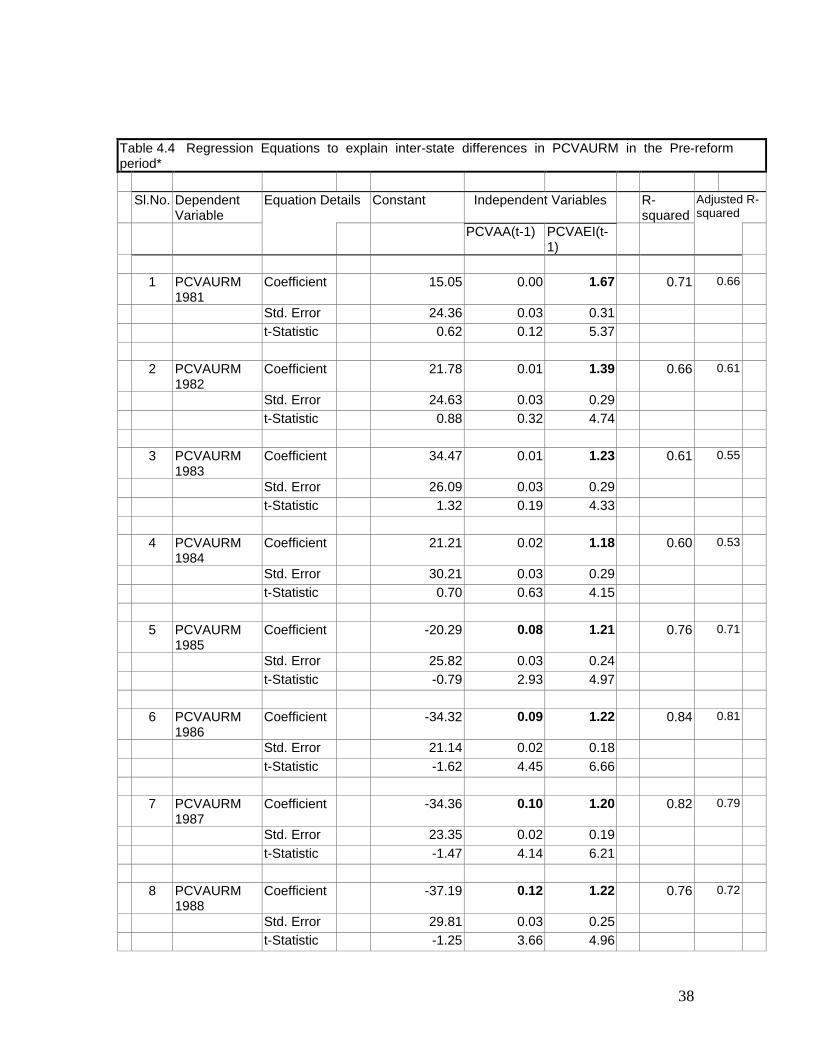
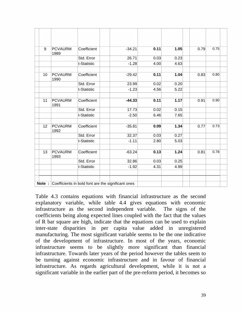
Note : Coefficients in bold font are the significant ones Table 4.3 contains equations with financial infrastructure as the second explanatory variable, while table 4.4 gives equations with economic infrastructure as the second independent variable. The signs of the coefficients being along expected lines coupled with the fact that the values of R bar square are high, indicate that the equations can be used to explain inter-state disparities in per capita value added in unregistered manufacturing. The most significant variable seems to be the one indicative of the development of infrastructure. In most of the years, economic infrastructure seems to be slightly more significant than financial infrastructure. Towards later years of the period however the tables seem to be turning against economic infrastructure and in favour of financial infrastructure. As regards agricultural development, while it is not a significant variable in the earlier part of the pre-reform period, it becomes so

40

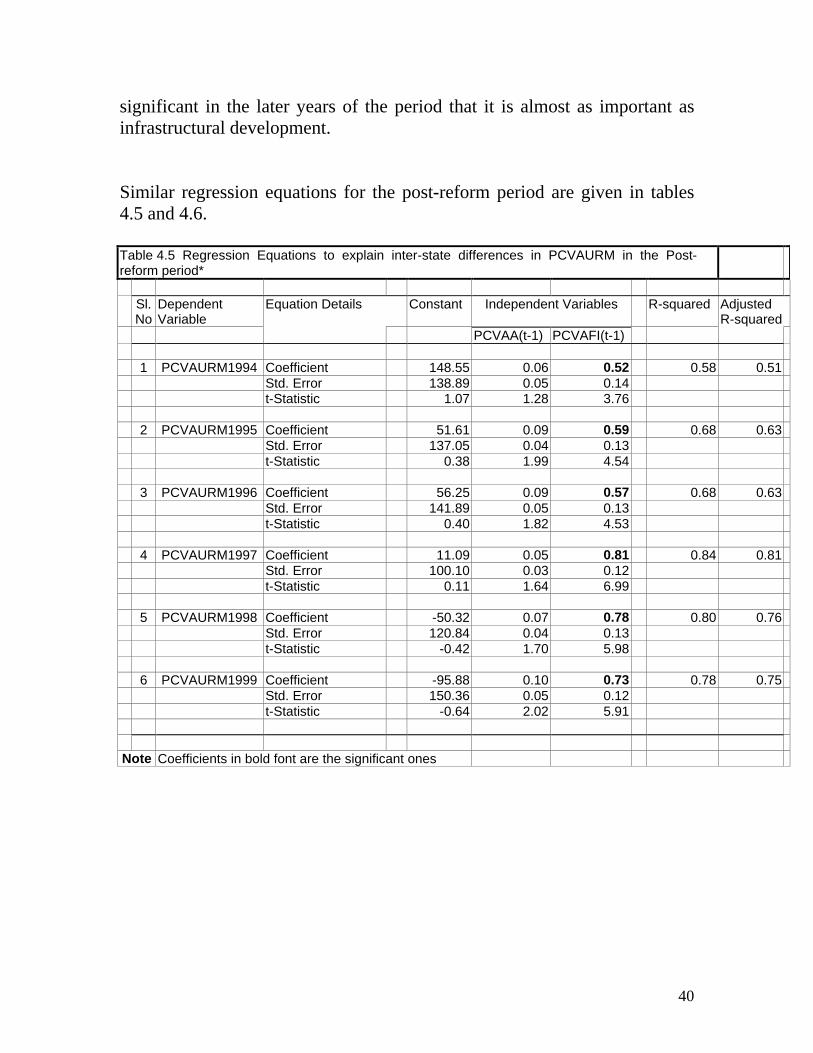
significant in the later years of the period that it is almost as important as infrastructural development. Similar regression equations for the post-reform period are given in tables 4.5 and 4.6. Table 4.5 Regression Equations to explain inter-state differences in PCVAURM in the Post-reform period*

Sl.No

Dependent Variable


PCVAA(t-1) PCVAFI(t-1) 1 PCVAURM1994 Coefficient 148.55 0.06 0.52 0.58 0.51 Std. Error 138.89 0.05 0.14 t-Statistic 1.07 1.28 3.76 2 PCVAURM1995 Coefficient 51.61 0.09 0.59 0.68 0.63 Std. Error 137.05 0.04 0.13 t-Statistic 0.38 1.99 4.54 3 PCVAURM1996 Coefficient 56.25 0.09 0.57 0.68 0.63 Std. Error 141.89 0.05 0.13 t-Statistic 0.40 1.82 4.53 4 PCVAURM1997 Coefficient 11.09 0.05 0.81 0.84 0.81 Std. Error 100.10 0.03 0.12 t-Statistic 0.11 1.64 6.99 5 PCVAURM1998 Coefficient -50.32 0.07 0.78 0.80 0.76 Std. Error 120.84 0.04 0.13 t-Statistic -0.42 1.70 5.98 6 PCVAURM1999 Coefficient -95.88 0.10 0.73 0.78 0.75 Std. Error 150.36 0.05 0.12 t-Statistic -0.64 2.02 5.91

Note Coefficients in bold font are the significant ones

41

Table 4.6 Regression Equations to explain inter-state differences in PCVAURM in the Post-reform period*

Sl.No

Dependent Variable


PCVAA(t-1) PCVAEI(t-1) 1 PCVAURM1994 Coefficient -34.19 0.02 1.28 0.74 0.69 Std. Error 122.18 0.04 0.23 t-Statistic -0.28 0.64 5.50 2 PCVAURM1995 Coefficient -95.37 0.05 1.25 0.78 0.74 Std. Error 124.00 0.04 0.21 t-Statistic -0.77 1.35 5.89 3 PCVAURM1996 Coefficient -99.39 0.05 1.16 0.78 0.74 Std. Error 128.76 0.04 0.20 t-Statistic -0.77 1.35 5.87 4 PCVAURM1997 Coefficient -51.33 0.04 1.08 0.83 0.80 Std. Error 107.29 0.03 0.16 t-Statistic -0.48 1.29 6.71 5 PCVAURM1998 Coefficient -92.38 0.08 0.91 0.80 0.77 Std. Error 122.55 0.04 0.15 t-Statistic -0.75 1.91 6.06 6 PCVAURM1999 Coefficient -68.70 0.03 1.08 0.80 0.76 Std. Error 144.20 0.05 0.18 t-Statistic -0.48 0.71 6.14


Table 4.5 contains equations with financial infrastructure as the second explanatory variable, while table 4.6 gives equations with economic infrastructure as the second independent variable. The signs of the coefficients are along expected lines and this coupled with the high values of R bar square indicates that the equations can be used to explain inter-state disparities in per capita value added in unregistered manufacturing. The only significant variable seems to be the one indicative of the development of infrastructure. In all years except one, economic infrastructure seems to be slightly more significant than financial infrastructure. But in striking contrast

42

with the pre-reform period, agricultural development does not seem to be a significant variable in any of the years considered. 4.3. Registered manufacturing

4.3.1Manner of change

Table 4.7 gives the values of the state relatives in per capita value added in registered manufacturing in the pre-reform period.

Table 4.7 State Relatives of Per Capita Value Added in Registered Manufacturing at 1980-81 Prices for the Pre-reform period*.

State Relatives for S.No State 1980-81

to 1982-83

1989-90 to 1991-

92

% change

(1) (2) (3) (4) (5) 1 Orissa 29.59 39.69 34.14 2 Bihar 36.79 40.80 10.89 3 Rajasthan 39.07 43.19 10.54 4 Uttar Pradesh 39.32 54.41 38.37 5 Assam 39.37 2723 -30.84 6 Madhya Pradesh 58.22 50.92 -12.54 7 Andhra Pradesh 61.43 79.39 29.24 8 Kerala 75.36 58.10 -22.90 9 Karnataka 84.01 102.50 22.00 10 Panjab 117.42 126.65 7.86 11 West Bengal 132.56 77.58 -41.48 12 Tamil Nadu 148.60 127.23 -14.38 13 Haryana 154.07 143.59 -6.80 14 Gujarat 192.65 184.34 -4.32 15 Maharshtra 280.11 255.79 -8.68

Note : *States are arranged in ascending order of the value of the state relative in the initial period, which refers to 1980-81 to 1982-83 . The terminal period refers to 1987-88 to 1989-90. Source of data is EPWRF..

The four better off states - Punjab, Haryana, Gujarat and Maharashtra belong to group one in this regard at both the beginning and the end of the period considered. Tamil Nadu is also in this category in the pre-reform era. West

43

Bengal and Karnataka change their respective groups during the period. West Bengal moves from group two to group one while Karnataka changes in the reverse direction. If we consider the signs of change, there are some indications of convergence during the period. Six out of nine states of group one at the beginning of the period experience positive changes. The two largest positive changes are both in less developed states - Uttar Pradesh and Orissa in that order. Five out of the six states of group two experience negative changes, the largest such change being in the state of West Bengal, with Kerala quite close on West Bengal's heels in this regard. One cannot however draw definite inferences on this count because while the coefficient of correlation between the value of the state relative at the beginning of the period and its % change during the period is negative, the value is only - 0.37, which is too small to be considered significant. The position is slightly different if we consider the post-reform period, results for which are given in Table 4.8.

Table 4.8 State Relatives of Per Capita Value Added in Registered Manufacturing at 1993-94 Prices for the Post-reform period*.

State Relatives for Sno State 1993-94 to

1995-96 1998-99 to 2000-2001

% change

(1) (2) (3) (4) (5) 1 Orissa 36.99 6.21 -83.22 2 Bihar 40.71 46.38 13.92 3 Assam 44.97 48.83 8.58 4 Uttar Pradesh 51.78 44.32 -14.41 5 Rajasthan 58.62 65.46 11.66 6 Kerala 61.24 70.57 15.23 7 West Bengal 63.14 71.42 13.12 8 Madhya Pradesh 66.00 79.62 20.64 9 Andhra pradesh 77.85 89.19 14.57 10 Karnataka 106.42 123.02 15.59 11 Punjab 152.76 157.40 3.03 12 Haryana 175.63 201.89 14.95 13 Tamil Nadu 192.20 177.85 -7.47 14 Gujarat 246.19 250.90 1.91 15 Maharashtra 246.94 248.88 0.79

Note : *States are arranged in ascending order of the value of the state relative in the initial period, which refers to 1993-94 to 1995-96 . The terminal period refers to 1998-1999 to 2000-2001.

Source : Calculated from Economic and Political Weekly Research

44

Foundation (EPWRF) (2002):Domestic Product of States of India 1960-61 to 2000-01.

There is no inter-group change between the states considered during the period. There are however some slight indications of divergence. A very large negative change - the largest for the period - occurs in the case of Orissa, which is in group one. Further five of the six states of group two also experience positive changes in their relatives during the period. But as against this, seven out of nine states of group one undergo positive changes during the period in the value of their relatives. It is also true that the largest positive change in this regard occurs in the case of Madhya Pradesh of group one. Nothing very definite can be said in this regard because while the coefficient of correlation between the value of the state relative at the beginning of the period and the % change in it during the period is positive, its value is only +0.11, which is not significant. The regression results for registered manufacturing for the pre-reform era are in tables 4.9 and 4.10. Table 4.9 Regression Equations to explain inter-state differences in PCVARM in the Pre-reform Period*

Sl.No

Dependent Variable Equation Details

Constant Independent Variables R-squared Adjusted R-squared

PCVAA(t-1) PCVAFI(t-1) 1 PCVARM 1981 Coefficient -47.57 0.08 2.91 0.77 0.73 Std. Error 46.41 0.06 0.48 t-Statistic -1.02 1.43 6.03 2 PCVARM 1982 Coefficient -43.36 0.08 2.79 0.74 0.70 Std. Error 51.00 0.06 0.50 t-Statistic -0.85 1.38 5.62 3 PCVARM 1983 Coefficient -33.33 0.07 2.78 0.71 0.66 Std. Error 58.41 0.07 0.53 t-Statistic -0.57 1.03 5.23 4 PCVARM 1984 Coefficient -31.09 0.09 2.42 0.71 0.66 Std. Error 61.55 0.07 0.47 t-Statistic -0.51 1.22 5.19 5 PCVARM 1985 Coefficient -57.87 0.11 2.59 0.71 0.66 Std. Error 65.06 0.08 0.51

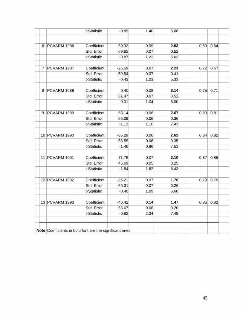
45

t-Statistic -0.89 1.40 5.08

6 PCVARM 1986 Coefficient -60.32 0.09 2.63 0.69 0.64 Std. Error 69.62 0.07 0.52 t-Statistic -0.87 1.22 5.03 7 PCVARM 1987 Coefficient -25.59 0.07 2.21 0.72 0.67 Std. Error 59.54 0.07 0.41 t-Statistic -0.43 1.03 5.33 8 PCVARM 1988 Coefficient 0.40 -0.08 3.14 0.75 0.71 Std. Error 61.47 0.07 0.52 t-Statistic 0.01 -1.04 6.00 9 PCVARM 1989 Coefficient -63.14 0.06 2.67 0.83 0.81 Std. Error 56.09 0.06 0.36 t-Statistic -1.13 1.10 7.43 10 PCVARM 1990 Coefficient -85.29 0.06 2.62 0.84 0.82 Std. Error 58.55 0.06 0.35 t-Statistic -1.46 0.96 7.53 11 PCVARM 1991 Coefficient -71.75 0.07 2.10 0.87 0.85 Std. Error 46.69 0.05 0.25 t-Statistic -1.54 1.62 8.43 12 PCVARM 1992 Coefficient -26.21 0.07 1.76 0.79 0.76 Std. Error 66.31 0.07 0.26 t-Statistic -0.40 1.09 6.68 13 PCVARM 1993 Coefficient -46.42 0.14 1.47 0.85 0.82 Std. Error 56.67 0.06 0.20 t-Statistic -0.82 2.34 7.48


46

Table 4.10 Regression Equations to explain inter-state differences in PCVARM in the Pre-reform period*

Sl.No

Dependent Variable Equation Details Constant Independent Variables R-squared Adjusted R-squared

PCVAA(t-1)

PCVAEI(t-1)

1 PCVARM 1981 Coefficient -85.61 0.05 3.91 0.81 0.78 Std. Error 43.84 0.05 0.56 t-Statistic -1.95 1.08 7.01 2 PCVARM 1982 Coefficient -90.00 0.05 3.92 0.86 0.84 Std. Error 39.59 0.04 0.47 t-Statistic -2.27 1.14 8.32 3 PCVARM 1983 Coefficient -67.48 0.06 3.56 0.72 0.67 Std. Error 60.95 0.07 0.67 t-Statistic -1.11 0.91 5.34 4 PCVARM 1984 Coefficient -73.24 0.06 3.53 0.89 0.88 Std. Error 38.21 0.04 0.36 t-Statistic -1.92 1.41 9.76 5 PCVARM 1985 Coefficient -110.17 0.10 3.68 0.89 0.87 Std. Error 41.47 0.05 0.39 t-Statistic -2.66 2.09 9.43 6 PCVARM 1986 Coefficient -111.54 0.10 3.46 0.79 0.76 Std. Error 60.53 0.06 0.53 t-Statistic -1.84 1.61 6.58 7 PCVARM 1987 Coefficient -91.32 0.11 3.05 0.81 0.77 Std. Error 54.21 0.06 0.45 t-Statistic -1.68 2.02 6.82 8 PCVARM 1988 Coefficient -65.85 0.07 3.49 0.85 0.83 Std. Error 51.52 0.05 0.42 t-Statistic -1.28 1.24 8.23 9 PCVARM 1989 Coefficient -69.32 0.06 3.67 0.90 0.88 Std. Error 43.55 0.04 0.37 t-Statistic -1.59 1.29 9.92

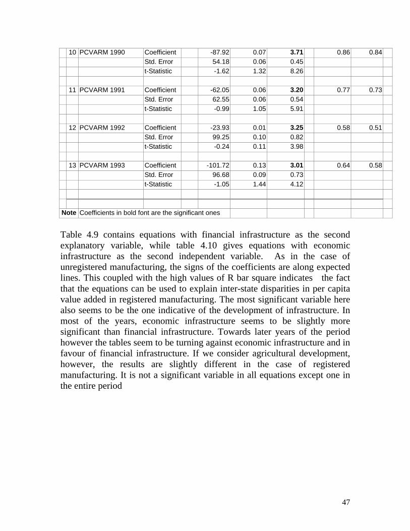
47

10 PCVARM 1990 Coefficient -87.92 0.07 3.71 0.86 0.84 Std. Error 54.18 0.06 0.45 t-Statistic -1.62 1.32 8.26 11 PCVARM 1991 Coefficient -62.05 0.06 3.20 0.77 0.73 Std. Error 62.55 0.06 0.54 t-Statistic -0.99 1.05 5.91 12 PCVARM 1992 Coefficient -23.93 0.01 3.25 0.58 0.51 Std. Error 99.25 0.10 0.82 t-Statistic -0.24 0.11 3.98 13 PCVARM 1993 Coefficient -101.72 0.13 3.01 0.64 0.58 Std. Error 96.68 0.09 0.73 t-Statistic -1.05 1.44 4.12

Note Coefficients in bold font are the significant ones Table 4.9 contains equations with financial infrastructure as the second explanatory variable, while table 4.10 gives equations with economic infrastructure as the second independent variable. As in the case of unregistered manufacturing, the signs of the coefficients are along expected lines. This coupled with the high values of R bar square indicates the fact that the equations can be used to explain inter-state disparities in per capita value added in registered manufacturing. The most significant variable here also seems to be the one indicative of the development of infrastructure. In most of the years, economic infrastructure seems to be slightly more significant than financial infrastructure. Towards later years of the period however the tables seem to be turning against economic infrastructure and in favour of financial infrastructure. If we consider agricultural development, however, the results are slightly different in the case of registered manufacturing. It is not a significant variable in all equations except one in the entire period

48

Regression results for the post-reform era are given in tables 4.11 and 4.12. Table 4.11 Regression Equations to explain inter-state differences in PCVARM in the Post-reform period* Sl

No Dependent Variable Equation

Details Constant Independent Variables R-squared Adjusted R-

squared PCVAA(t-1) PCVAFI(t-1) 1 PCVARM1994 Coefficient 44.14 0.16 1.12 0.65 0.59 Std. Error 264.28 0.09 0.26 t-Statistic 0.17 1.84 4.27 2 PCVARM1995 Coefficient -110.57 0.19 1.31 0.73 0.68 Std. Error 271.82 0.09 0.26 t-Statistic -0.41 2.24 5.05 3 PCVARM1996 Coefficient -57.54 0.18 1.22 0.62 0.56 Std. Error 339.90 0.11 0.30 t-Statistic -0.17 1.59 4.03 4 PCVARM1997 Coefficient -142.07 0.15 1.45 0.72 0.67 Std. Error 271.95 0.09 0.32 t-Statistic -0.52 1.70 4.58 5 PCVARM1998 Coefficient -253.67 0.16 1.47 0.73 0.69 Std. Error 278.28 0.09 0.30 t-Statistic -0.91 1.68 4.87 6 PCVARM1999 Coefficient -313.31 0.24 1.13 0.72 0.67 Std. Error 301.53 0.10 0.25 t-Statistic -1.04 2.44 4.56 Note Coefficients in bold font are the significant

ones

49

Table 4.12. Regression Equations to explain inter-state differences in PCVARM in the Post-reform period* Sl.No. Dependent

Variable Equation Details Constant Independent Variables R-squared Adjusted

R-squared PCVAA(t-1) PCVAEI(t-1) 1 PCVARM1994 Coefficient -241.77 0.10 2.38 0.64 0.59 Std. Error 298.51 0.09 0.57 t-Statistic -0.81 1.08 4.20 2 PCVARM1995 Coefficient -378.37 0.12 2.57 0.74 0.69 Std. Error 288.86 0.09 0.50 t-Statistic -1.31 1.40 5.19 3 PCVARM1996 Coefficient -365.66 0.12 2.41 0.68 0.63 Std. Error 340.57 0.11 0.52 t-Statistic -1.07 1.09 4.59 4 PCVARM1997 Coefficient -287.65 0.12 2.03 0.77 0.73 Std. Error 254.08 0.08 0.38 t-Statistic -1.13 1.56 5.35 5 PCVARM1998 Coefficient -352.68 0.17 1.76 0.77 0.73 Std. Error 263.70 0.09 0.32 t-Statistic -1.34 1.95 5.45 6 PCVARM1999 Coefficient -305.95 0.13 1.78 0.80 0.77 Std. Error 250.19 0.09 0.30 t-Statistic -1.22 1.48 5.87 Note : Coefficients in bold font are the significant ones

Table 4.11 contains equations with financial infrastructure as the second explanatory variable, while table 4.12 gives the results with economic infrastructure as the second independent variable. The signs of the coefficients are along expected lines and this coupled with the high values of R bar square indicates that the equations can be used to explain inter-state disparities in per capita value added in registered manufacturing in the post-reform era. The more significant variable seems to be the one indicative of the development of infrastructure. In all years except one, economic infrastructure seems to be slightly more significant than financial infrastructure. But in striking contrast with the pre-reform period, agricultural development does not seem to be a significant variable in ten of the twelve equations presented.

50

4.4 Total Manufacturing 4.4.1 Manner of Change State relatives in per capita value added in total manufacturing in the pre-reform period are given in Table 4.13 table 4.13

Table 4.13 State Relatives of Per Capita Value Added in Total Manufacturing at 1980-81 Prices for the Pre-reform period*.

State Relatives for Rank States 1980-81 to

1982-83 1989-90 to 1991-92 % change

(1) (2) (3) (4) (5) 1 Assam 32.03 21.92 -31.56 2 Orissa 39.59 39.70 0.29 3 Bihar 44.69 42.69 -4.48 4 Uttar Pradesh 45.53 53.18 16.80 5 Rajasthan 48.38 45.07 -6.83 6 Madhya

Pradesh 57.81 51.32 -11.22

7 Andhra Pradesh 59.56 72.60 21.90 8 Karnataka 72.38 82.19 13.56 9 Kerala 76.63 61.70 -19.49 10 Punjab 115.86 133.62 15.33 11 Haryana 119.66 146.82 22.69 12 West Bengal 124.66 85.11 -31.73 13 Gujarat 144.16 148.64 3.11 14 Tamil Nadu 144.52 111.81 -22.63 15 Maharashtra 219.16 209.79 -4.28

Note: *States are arranged in ascending order of the value of the state relative in the initial period, which refers to 1980-81 to 1982-83 . The terminal period refers to 1989-90 to 1991-92. Total Manufacturing covers Registered and Unregistered Manufacturing.

Source: Calculated from Economic and Political Weekly Research Foundation (EPWRF) (2002): Domestic Product of States of India 1960-61 to 2000-01

The most noticeable feature here seems to be the relative decline in this regard of the state of West Bengal, which shifts from group two in the

51

beginning to group one towards the end of the period. In fact West Bengal experiences the largest decline of this kind, with Assam, which has the lowest value for the state relative in the entire period, a very close second. Four out of nine states of group one experience increases in their relatives while three out of six states of group two in the beginning of the period undergo negative changes.The largest increase however occurs in the case of Haryana which is in group one in both the periods. Nothing very definite can be inferred about convergence or divergence because the coefficient of correlation between the relative at the beginning of the period and its % change is just - 0.03 and is not significant. The picture in this regard for the post-reform period can be obtained from the data given in table 4.14 and is slightly different from the pre-reform one.

Table 4.14 State Relatives of Per Capita Value Added in Total Manufacturing at 1993-94 Prices for the Post-reform period*.

State Relatives for

S.no State 1993-94 to 1995-96

1998-99 to 2000-2001

% change

(1) (2) (3) (4) (5)

1 Orissa 32.40 10.79 -66.70

2 Bihar 32.76 34.01 3.82

3 Assam 38.11 38.20 0.24

4 Uttar Pradesh 55.78 48.31 -13.40

5 Rajasthan 68.09 69.85 2.58

6 Madhya Pradesh

73.75 79.53 7.84

7 Andhra Pradesh 80.11 87.17 8.81

8 Kerala 80.58 76.85 -4.63

9 West Bengal 86.87 95.32 9.72

10 Karnataka 111.78 121.87 9.03

11 Punjab 146.28 146.72 0.30

12 Haryana 170.32 182.38 7.08

13 Tamil Nadu 196.82 176.66 -10.25

14 Gujarat 231.23 240.76 4.12

15 Maharashtra 235.67 233.40 -0.96

Note : *States are arranged in ascending order of the value of the state relative in the initial period, which refers to 1993-94 to 1995-96 . The terminal period refers to 1998-1999 to 2000-2001.Total Manufacturing covers Registered and Unregistered Manufacturing.

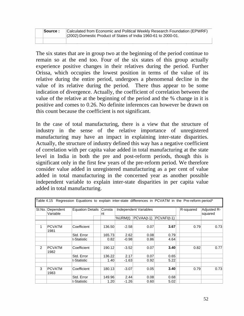
52

Source : Calculated from Economic and Political Weekly Research Foundation (EPWRF) (2002):Domestic Product of States of India 1960-61 to 2000-01.

The six states that are in group two at the beginning of the period continue to remain so at the end too. Four of the six states of this group actually experience positive changes in their relatives during the period. Further Orissa, which occupies the lowest position in terms of the value of its relative during the entire period, undergoes a phenomenal decline in the value of its relative during the period. There thus appear to be some indication of divergence. Actually, the coefficient of correlation between the value of the relative at the beginning of the period and the % change in it is positive and comes to 0.26. No definite inferences can however be drawn on this count because the coefficient is not significant. In the case of total manufacturing, there is a view that the structure of industry in the sense of the relative importance of unregistered manufacturing may have an impact in explaining inter-state disparities. Actually, the structure of industry defined this way has a negative coefficient of correlation with per capita value added in total manufacturing at the state level in India in both the pre and post-reform periods, though this is significant only in the first few years of the pre-reform period. We therefore consider value added in unregistered manufacturing as a per cent of value added in total manufacturing in the concerned year as another possible independent variable to explain inter-state disparities in per capita value added in total manufacturing. Table 4.15 Regression Equations to explain inter-state differences in PCVATM in the Pre-reform period* Sl.No. Dependent

Variable Equation Details Consta

nt Independent Variables R-squared Adjusted R-

squared %URM(t) PCVAA(t-1) PCVAFI(t-1)

1 PCVATM 1981

Coefficient 136.50 -2.58 0.07 3.67 0.79 0.73

Std. Error 165.73 2.62 0.08 0.79 t-Statistic 0.82 -0.98 0.86 4.64

2 PCVATM 1982

Coefficient 190.12 -3.52 0.07 3.40 0.82 0.77


3 PCVATM 1983

Coefficient 180.13 -3.07 0.05 3.40 0.79 0.73


53

4 PCVATM

1984 Coefficient 197.80 -4.13 0.10 2.96 0.76 0.70


5 PCVATM

1985 Coefficient 150.73 -4.60 0.19 3.05 0.78 0.72


6 PCVATM

1986 Coefficient 131.32 -4.50 0.19 3.13 0.77 0.70


7 PCVATM 1987

Coefficient 90.61 -2.97 0.16 2.86 0.76 0.70


8 PCVATM 1988

Coefficient 50.16 -1.80 0.01 4.11 0.76 0.69


9 PCVATM 1989

Coefficient -36.83 -1.79 0.18 3.36 0.85 0.81

Std. Error 170.29 4.47 0.08 0.54 t-Statistic -0.22 -0.40 2.21 6.23

10 PCVATM

1990 Coefficient -11.57 -2.34 0.18 3.11 0.85 0.81


11 PCVATM

1991 Coefficient -44.85 -1.68 0.21 2.68 0.89 0.86


12 PCVATM 1992

Coefficient 75.84 -3.56 0.20 2.34 0.85 0.81


13 PCVATM 1993

Coefficient 58.94 -3.62 0.29 1.93 0.91 0.88



54

Table 4.16 Regression Equations to explain inter-state differences in PCVATM in the Pre-reform period*

Sl.No.

Dependent Variable

Equation Details Constant Independent Variables R-squared

Adjusted R-squared

%URM(t) PCVAA(t-1) PCVAEI(t-1)

1 PCVATM 1981 Coefficient -40.08 -0.50 0.05 5.46 0.84 0.80 Std. Error 158.73 2.40 0.07 0.94 t-Statistic -0.25 -0.21 0.78 5.80 2 PCVATM 1982 Coefficient -197.82 2.07 0.07 5.87 0.88 0.84 Std. Error 150.56 2.25 0.06 0.87 t-Statistic -1.31 0.92 1.21 6.71 3 PCVATM 1983 Coefficient 14.53 -0.81 0.06 4.63 0.76 0.70

Std. Error 185.15 2.86 0.09 1.01 t-Statistic 0.08 -0.28 0.68 4.58 4 PCVATM 1984 Coefficient -148.01 1.88 0.09 5.00 0.89 0.86 Std. Error 144.73 2.62 0.06 0.66

t-Statistic -1.02 0.72 1.43 7.60 5 PCVATM 1985 Coefficient -219.31 1.78 0.18 5.18 0.91 0.88 Std. Error 142.67 2.63 0.06 0.67 t-Statistic -1.54 0.68 2.95 7.72

6 PCVATM 1986 Coefficient -48.60 -2.01 0.20 4.42 0.85 0.81 Std. Error 159.43 2.96 0.07 0.72 t-Statistic -0.30 -0.68 2.71 6.10 7 PCVATM 1987 Coefficient -103.71 -0.51 0.21 4.21 0.86 0.82 Std. Error 158.15 3.32 0.07 0.63 t-Statistic -0.66 -0.15 3.05 6.72 8 PCVATM 1988 Coefficient -189.89 2.31 0.17 4.88 0.86 0.82

Std. Error 153.83 3.66 0.08 0.65 t-Statistic -1.23 0.63 2.11 7.49 9 PCVATM 1989 Coefficient -247.80 4.08 0.13 5.09 0.90 0.88 Std. Error 150.15 3.89 0.07 0.62

t-Statistic -1.65 1.05 1.91 8.21

10 PCVATM 1990 Coefficient -80.14 -0.92 0.19 4.66 0.90 0.88 Std. Error 147.22 3.29 0.07 0.61 t-Statistic -0.54 -0.28 2.82 7.58

11 PCVATM 1991 Coefficient 69.13 -4.91 0.21 4.10 0.88 0.84 Std. Error 137.20 3.35 0.07 0.61 t-Statistic 0.50 -1.46 3.03 6.74

55

12 PCVATM 1992 Coefficient 204.19 -7.22 0.14 4.28 0.69 0.61 Std. Error 250.58 5.95 0.12 1.04 t-Statistic 0.81 -1.21 1.13 4.10

13 PCVATM 1993 Coefficient 107.17 -6.90 0.29 3.89 0.75 0.69 Std. Error 251.89 5.71 0.11 0.93

t-Statistic 0.43 -1.21 2.55 4.17 Note: Coefficients in bold font are the significant ones

Tables 4.15 and 4.16 give the results for the pre-reform era with three possible explanatory variables indicative of the structure of industry, and the development of agriculture and infrastructure respectively, with table 4.15 considering the financial aspect and table 4.16 considering the economic aspect as defined here. The results indicate that infrastructural development has a salutary impact on industrial development. In fact it is the most significant explanatory variable with economic infrastructure being by and large more so than financial infrastructure. As regards agricultural development as considered here, it also has a favourable impact on industry. Actually this variable seems to become also significant in the later years of the pre-reform period. If we consider the structure of industry as indicated by the relative importance of unregistered manufacturing in total manufacturing, it is not a significant explanatory variable in any of the equations nor are the signs of the coefficient of this variable the same at different points of time in the pre-reform period Tables 4.17 and 4.18 give similar for the post-reform period, with table 4.17 considering the financial aspect and table 4.18 considering the economic aspect as defined here. Table 4.17 Regression Equations to explain inter-state differences in PCVATM in the Post-reform period*

Sl.No.

Dependent Variable

Equation Details Constant Independent Variables R-squared

Adjusted R-squared

%URM(t) PCVAA(t-1) PCVAFI(t-1)

1 PCVATM1994 Coefficient 99.85 2.49 0.22 1.64 0.66 0.56 Std. Error 782.22 18.02 0.13 0.39 t-Statistic 0.13 0.14 1.68 4.17 2 PCVATM1995 Coefficient -31.06 -0.81 0.28 1.90 0.75 0.68 Std. Error 642.59 14.84 0.13 0.38 t-Statistic -0.05 -0.05 2.24 5.06

56

3 PCVATM1996 Coefficient 517.65 -14.56 0.27 1.81 0.68 0.59 Std. Error 915.94 22.08 0.16 0.42 t-Statistic 0.57 -0.66 1.72 4.32 4 PCVATM1997 Coefficient 727.27 -22.79 0.18 2.33 0.81 0.76 Std. Error 685.64 15.86 0.11 0.39 t-Statistic 1.06 -1.44 1.66 5.91 5 PCVATM1998 Coefficient 197.04 -11.58 0.22 2.20 0.80 0.74 Std. Error 559.99 9.69 0.12 0.40 t-Statistic 0.35 -1.19 1.74 5.46 6 PCVATM1999 Coefficient 85.88 -13.16 0.32 1.91 0.78 0.72 Std. Error 706.19 14.89 0.14 0.36 t-Statistic 0.12 -0.88 2.33 5.34

Note: Coefficients in bold font are the significant ones

Table 4.18 Regression Equations to explain inter-state differences in PCVATM in the Post-reform

period*

Sl.No.

Dependent Variable


%URM(t) PCVAA(t-1)

PCVAEI(t-1)

1 PCVATM1994 Coefficient 280.89 -16.20 0.11 3.83 0.73 0.65 Std. Error 689.73 16.47 0.12 0.77 t-Statistic 0.41 -0.98 0.88 4.98 2 PCVATM1995 Coefficient -136.03 -10.45 0.17 3.91 0.80 0.74 Std. Error 579.41 13.47 0.12 0.67 t-Statistic -0.23 -0.78 1.50 5.87 3 PCVATM1996 Coefficient 425.03 -25.96 0.17 3.69 0.78 0.71 Std. Error 766.86 18.62 0.13 0.66 t-Statistic 0.55 -1.39 1.28 5.61 4 PCVATM1997 Coefficient 594.79 -25.10 0.14 3.24 0.86 0.82 Std. Error 603.90 13.98 0.10 0.47 t-Statistic 0.98 -1.80 1.47 6.96 5 PCVATM1998 Coefficient 257.77 -16.84 0.23 2.67 0.86 0.82 Std. Error 466.78 8.13 0.10 0.39 t-Statistic 0.55 -2.07 2.16 6.81 6 PCVATM1999 Coefficient 219.97 -15.83 0.14 2.97 0.85 0.81 Std. Error 586.21 12.45 0.12 0.44 t-Statistic 0.38 -1.27 1.16 6.79

57

Note: Coefficients in bold font are the significant ones

The results indicate that in the post-reform period too, infrastructural development has a salutary impact on industrial development. It continues to remain the most significant explanatory variable with economic infrastructure being clearly more so than financial infrastructure. If we look at the signs of the coefficients, agricultural development seems to have a favourable impact on industry The coefficient of this variable is however not significant in most of the years of the post-reform period nor is there any tendency for it to increase in significance over time. The structure of industry as defined here continues to be a variable that is not significant, but the signs of the coefficients are in all cases except one negative indicating that the states with a larger share in value added in small scale manufacturing seem to be the ones which are less developed in terms of total manufacturing in the post-reform period. 4.5 Inferences As regards unregistered manufacturing, the study here indicates that while there are no clear signs of convergence or divergence of inter-state disparities of per capita value added in the pre-reform era, there are some indications of divergence in the post-reform period. Particularly interesting are the relative declines in West Bengal and in Kerala in the pre and post reform periods respectively making the states switch groups during these periods. The phenomenal improvement in Haryana in the pre-reform period also deserves special notice. If we consider the possible explanatory factors for inter-state differences in per capita value added in unregistered manufacturing, infrastructural development emerges as the most important one. Within infrastructure, economic infrastructure in terms of transport, communication and storage seems to play a more important role in most of the years considered As regards the development of agriculture as reflected by per capita value added in agriculture proper, it does seem to have a salutary effect on per capita value added in unregistered manufacturing, particularly in the later years of the pre-reform era. But this explanatory variable pales into insignificance in comparison with variables indicative of infrastructural development in the post-reform period. In the case of registered manufacturing, there are some indications of convergence in inter-state disparities in per capita value added in the pre-

58

reform period. West Bengal undergoes relative decline in this regard so much so that it switches from group two at the beginning to group one at the end with the reverse happening in the case of Karnataka. But the state of Kerala belonging to group one actually experiences the largest decline. The net result is that the signs of convergence are not very definite ones. In contrast, in the post-reform period, there are hardly any indications of convergence or divergence, other than the noticeable relative improvement in the case of the state of Madhya Pradesh. There is no shift in states between groups during the period. Infrastructural development again comes out to be the more significant of the explanatory variables considered in both the pre and post-reform periods. Within infrastructural development economic infrastructure seems slightly more effective in this regard than financial infrastructure except in the later years of the pre-reform era. Agricultural development does not seem to be an important variable in explaining inter-state disparities in registered manufacturing in both the periods. If we consider total manufacturing, taking into account both unregistered and registered manufacturing together, there is no noticeable tendency towards convergence or divergence in per capita value added in total manufacturing. This is true irrespective of whether we consider the pre-reform or the post-reform period. The noticeable features seem to be the big decline in the relative position of West Bengal in the pre-reform period and that of Orissa in the post-reform one. As regards the factors explaining inter-state differences in per capita value added in manufacturing, such differences in infrastructural development as indicated by value added in the sector, seems the most important one. Within infrastructure, transport and communication seem more important in this regard than banking and insurance. While there are indications of agricultural development having a favourable and significant impact on industrial development at the state level particularly in the later part of the pre-reform era, there is no such indication in this regard in the post-reform years. As regards the structure of industry in terms of value added in unregistered manufacturing as per cent of value added in total manufacturing, there are no indications of any definite impact of this on industrial development in the pre-reform era, there are some signs in the post-reform years that the more developed total manufacturing is in a state, the less the relative importance of unregistered manufacturing

59

Chapter 5: Main Findings / Conclusions The preliminary analysis here on the basis of the latest available data gives some broad indications regarding India’s regional development experience in the two decades since the eighties. It seems to substantiate the view that the pattern of regional economic change depends upon the indicator of economic development considered as has been argued in the multi-pattern hypothesis in this regard. As regards per capita NSDP, while there are no definite indications of either divergence or convergence at the regional level in the pre-reform era whereas if we consider indicators of levels of living, there are signs of inter-state convergence in the pre-reform period. If we consider the post-reform period, the evidence here points towards some indications of inter-state divergence in terms of per capita NSDP along with very definite evidence in this regard in terms of the indicators of levels of living. It has of course to be borne in mind that we have looked at convergence and divergence in a non-econometric sense and not examined sigma or beta convergence which involve inter-temporal analysis of sinle summary measures of inter-regional dispersion and relationship between rates of growth and base year values of the indicator under study for the different regions respectively. Besides lending credence to findings on the basis of much earlier data by many including Nair (1982) from the fifties to the eighties, the evidence here seems to be in line also with the results of some detailed studies using data for recent years like the ones by Dholakia(2003), Shetty (2003) and Bhattacharya and Sakthivel (2004). Recent econometric studies using data for much longer periods also seem to lead to similar inferences. Das (2002) compares interstate movements in real wage rates in agriculture between the years 1956-57 to 1992-93 to infer that there are no indications of continued divergence with some indications also of convergence. Shaban (2002) on the other hand finds clear indications of divergence on the basis of his analysis of data on per capita NSDP between the years 1960-61 to 1996-97. . A broad comparison between the pre and post-reform periods in our study also reveals some interesting facets of regional change. If we consider per capita NSDP, there is evidence about these diverging in a much more

60

noticeable manner between the states considered here in the post-reform period in striking contrast with that in the pre-reform era. According to some, including Cassen (2002), this need not cause much concern since regional divergence in per capita NSDP has been a tendency prevalent in India since the 50’s. One is however constrained to dispute such a contention. This is so because on the basis of very detailed regional analysis, many in India, including Dholakia (1985) and Nair (1982) hold the view that India had almost reached the turning point of the concentration-cycle hypothesis in this regard by the late 70’s. Further, there is some evidence in this study to prove that there has not been much regional divergence in this regard between the 80’s and the 90’s.In view of all this, the noticed regional divergence in per capita NSDP the post-reform period since the 90’s should be a matter of some concern. The disaggregated sectoral analysis of regional change here seems to hold some insights in this regard. Manufacturing industry has, almost since times immemorial, been looked upon as the panacea for the development of the backward regions in all parts of the world including India. Attention in this regard often gets focused on large scale industry or registered manufacturing value added in which forms around 60% of the value added in total manufacturing at the all India level. In the case of registered or large scale manufacturing, while there were some indications of inter-state convergence in the pre-reform period, there is no definite evidence either way for the post-reform one. If we consider small scale or unregistered manufacturing, while there are no signs of convergence or divergence in the pre-reform period, there are more definite signs of divergence in the post-reform one. As regards, regional disparities in agriculture and allied sectors, while there seems to have been some inter-state convergence in the pre-reform era, there are no indications of either kind in the post-reform era A matter of even greater concern is the evidence here that the tendency towards regional convergence in levels of living in the pre-reform period has been arrested and in some cases even reversed in the post-reform period. This is all the more so because one of the strongest theoretical arguments put forth in favor of liberalizing the Indian economy was that though economic growth did take place in the Indian economy, it did not trickle down adequately in both inter-regional and inter-personal terms. It is true that there is some evidence of reduction in inequalities and of poverty at the personal level and also at the sub-state level as pointed out by Singh etc. al (2003) and Sunderam and Tendulkar(2003). Some consolation may emerge

61

from the fact that if we consider the HDI, the tendency seems to be of convergence in both the pre and post-reform periods. A closer look at the evidence in this regard, however, offers poor solace since there are large declines in relatives in HDI in those states of India, that are at the bottom from the point of view of almost all indicators of economic development. There seems to be a link between the overall pattern of regional change and the sectoral results in this regard. The comparison of the results regarding the relationship between the growth of NSDP and employment at the regional level, between the pre and the post-reform periods gives a broad indication about such a logical connection. While growth of employment and of NSDP had a positive and significant correlation in the pre-reform era, there is some evidence almost pointing to the contrary for the post-reform era. This need not lead to any raised eyebrows because agriculture and unregistered manufacturing are the two sectors having a tremendous impact on the growth of employment of people in the region and hence on income accruing to people in most state economies in India. In the agricultural sector, there is no evidence of any inter-state convergence in the post-reform era. As regards unregistered manufacturing, there seems on the contrary a definite tendency towards inter-state divergence in the post-reform period. Of course much more detailed and in-depth work needs to be done possibly along the lines of Datt and Ravillion (2002) before more definite inferences can be drawn in this connection.. There is evidence in the study to suggest that infrastructural development is of great help in promoting regional development. This is particularly true if we consider an indicator of level of living like HDI and seems true to some extent also in the case of per capita NSDP. A detailed analysis of the development of industry at the state level in India also indicates that infrastructural development is particularly helpful for the development of both registered and unregistered manufacturing There are also two other indications with interesting policy implications. One is the already accepted finding that agricultural development is beneficial for the development of unregistered manufacturing at the regional level. The other is the interesting hint here that measures to reduce poverty in a region do not always go against the objective of improving the relative position of a region in terms of its per capita net domestic product. Much more work possibly with the help of causality tests and along the lines also of Datt and Ravilion(2002) needs to be done before more definite policy inferences can be drawn in this regard.

62

References

Bhattacharya, B.B and S. Sakthivel (2004), Regional Growth and Disparity in India, Economic and Political Weekly, (EPW), March 6, pp1071-1077

Booth, E.J.R (1964), “ Inter-regional Income Differences”, Southern Economic Journal (SEJ), Vol 31, No 1, July, pp 44-51 Cassen, R.H (2002), “Well-Being in the 90’s : Towards a Balance Sheet”, EPW, Vol 37, No 27, pp 2789-2794 Das, T.K(2002), “Convergence Across Indian States: Cross-Sectional and Panel Estimations”, South Asia Economic Journal, Volume 3, No 2, pp227-239 Datt,G and M.Ravallion(2002), “Is India’s Economic Growth Leaving the Poor Behind?”. Mimeographed paper at World Bank Workshop on Poverty Estimates, New Delhi, January Dholakia, R.H (1985), Regional Disparity in Economic growth in India, Himalaya, New Delhi. -------------------------,(2003), Regional Disparity in Economic and Human Development in India, RBI Chair Lecture, IIM, Ahmedabad Hanna, F.A (1959), State Income Differentials 1919-1954, Duke University Press, Durham Hirschman, Albert. O (1961), The Strategy of Economic Development, Yale University Press, New Haven. Hughes, R.B (1961), “ Inter-regional Income Differences: Self-Perpetuation”, Southern Economic Journal,Vol 28, No 1, July, pp 41-45. Kurian, N.J (2000), “ Widening Regional Disparities in India: Some Indicators” , EPW, Vol. 35, No 7, pp 538-55.

63

Malhotra, Rajeev (1998), An Interpretation of the Capability Approach for constructing developmental and Deprivational Indices- A Comparison of Alternative Estimates at Regional level for India (Mimeographed) Myrdal, G (1958), Economic Theory and Underdeveloped Regions, Vora, Bombay Nair, K.R.G (1982), Regional Experience in a Developing Economy, Wiley-Eastern, New Delhi -------------(1993a) Regional Economics: A Survey Report, Indian Council of Social Science Research, New Delhi -------------(1993 b), “ The New Economic Policy and the Development of Backward Regions: A Note On Orissa”,EPW, Vol 28, No 19, pp 939-941 Perloff, H.S, E.S. Dunn Jr, E.E.Lampard and R.F. Muth, (1960), Regions, Resources and Economic Growth, Resources for the Future, Johns Hopkins Press, Baltimore. Planning Commission (2002), National Human Development Report 2001, Government of India, New Delhi Sala-i-Martin (1996), “ Regional Cohesion: Evidence and Theories of Regional growth and Convergence”, European Economic Review, Vol 40, pp1325-1352 Shetty, S.L (2003), “ Growth of SDP and Structural Changes in State Economies:Inter-State Comparisons “, EPW,Vol 38, No 49, December 6, pp5189-5200 Shaban, Abdul (2002), “Growth and Disparities of Incomes Across States”, Man and Development, September , pp31-47 Singh, Nirvikar, L. Bhanadari, A. Chen and a. Khare, (2003), “Regional Inequality in India: A Fresh Look”, EPW,Vol 38, No 11, March 15, pp 1069-1073 Sundaram, K and S.D. Tendulkar(2003), “Poverty in India in the 1990s” , EPW, Vol 38, No 14, april 5, pp 1385-1394

64

Williamson, J.G (1963), “ Regional Inequality and the Process of National Development”, Economic Development and Cultural Change, Vol 13, No 4, Part II, July

Economic Reforms and Regional Disparities in Economic and...

Documents

Transcript of Economic Reforms and Regional Disparities in Economic and...