--

48 Transportation Research Record 870

Economic Impacts of Petroleum Shortages and Implications

for the Freight Transportation Industry

LARRY R. JOHNSON, RITA E. KNORR, CHRISTOPHER L. SARICKS, AND VEENA B. MENDIRATTA

The major economic impacts that result from petroleum supply interruptions and the subsequent effects on the demand for freight transportation are de­scribed. The analysis involved a simulation of the effects of three different levels of fuel supply shortfall on intercity freight transportation. The research included the use of three economic and transportation models to simulate the economic impacts of oil shortfalls and the resulting change in freight transpor­tation demand as expressed in tons shipped, ton miles of travel, and fuel use. Economic effects are discussed for a base case and then for 7, 14, and 23 per­cent petroleum shortfalls. The demand for freight transportation is determined by the output of various commodity sectors that generate traffic for the truck, rail, water, air, and pipeline modes. The effects of various diesel fuel price levels are also examined. The analysis suggests that at low, or controlled, fuel prices the more significant impacts for freight movements will be the reduction in output in the bulk commodity sectors, which are dominated by the waterway and rail modes. At high fuel prices (i.e., equilibrium levels), shipping is signifi­cantly decreased in all commodity sectors, but modal shifts are likely to occur from truck to rail and even from rail to water in some corridors.

The United States has experienced significant eco­nomic problems associated with two of the three major interruptions in the world supply of petro­leum--the Arab oil embargo in 1973-1974 and the Iranian revolution in 1979. Less difficulty was encountered with the loss of crude oil due to the Iran-Iraq war. High inventories coupled with re­duced demand have made the loss of those supplies barely noticeable. Saudi Arabia increased its oil production to partially compensate for a reduction in the oil spot-market pr ice in order to eventually produce a unified Organization of Petroleum Export­ing Countries (OPEC) pr ice. Competing economic and political goals in the Middle East cause this region to remain volatile, which suggests that future dis­ruptions in petroleum supply are highly probable, if not inevitable.

Petroleum supply shortages produce economic shocks that have a direct effect on the demand for freight transportation. However, the changes in economic activity are not uniform. Some sectors show a dramatic decline in production and sales that goes far beyond the level of the oil shortage, whereas others show no adverse impact or even some moderate gain. To quantify these economic changes, an econometi: ic model and two freight transportation models were used to simulate the effects of three different shortage situations. This section pro­vides a brief discussion of the modeling process. A description of the control forecast and three hypo­thetical oil shortfall cases simulated by the models is included in the following section.

The Data Resources, Inc. (DRI), Quarterly Model of the U.S. Economy has been used in this study to analyze the impacts of petroleum shortfalls at the national level. The ORI model is a simultaneous­equations model that includes a circular flow of income and expenditure in the economy.

The DRI model provided macroeconomic indicators for the Argonne National Laboratory Freight Respon­sive Accounting for Transportation Energy (FRATE) model to estimate the change in commodities shipped by mode before any contingency actions are initi­ated. The FRATE model calculates annual ton miles of travel (TMT) for commodities, accounts for modal activity, and computes the transportation energy consumed based on economic-sector output levels.

The base-year ton-mile estimates for the economic

sectors in FRATE are derived from the U.S. Bureau of the Census Commodity Transportation Survey (!.l· The FRATE economic activity sectors are paired with similar sectors in the DRI econometric model in order to apply the projected output growth rates to the base-year ton-mile estimates (1_). The model assumes, for lack of a better indicator, that ton­mile growth is directly related to output growth rates. Traffic estimates for truck, railroad, marine, air, and pipeline modes are calculated based on historic modal-split distributions (1,3-5).

Energy intensity values associated ;-ith -each eco­nomic sector are based on the freight mode and the type of service provided by that mode (}_,_!,il. The FRATE economic-sector ton-mile estimates are applied to the energy intensity values for projected energy consumption values. FRATE then aggregates the energy demand of all sectors by type of mode.

The third model used in this analysis was the National Freight Demand Model (NAFDEM), developed for Argonne National Laboratory by the Massachusetts Institute of Technology. NAFDEM provides a means to determine shipper response to rate and level-of­service alterations imposed by carriers during fuel shortfall situations. This response could involve a change in the freight mode selected for shipment, a change in the size of shipment, or both. The logic governing the degree and direction of change arises from a utility logit model of freight mode and ship­ment size developed and calibrated to observed shipper behavior by Chiang and others (2). NAFDEM does not include the pipeline mode since it is not applicable for most commodity sectors.

A basic premise of NAFDEM is that shippers in any commodity group seek to move more freight by the mode or modes that maximize their total utility. This utility is computed from the mode-specific rate and level-of-service relations to commodity charac­ter is tics developed by Chiang. NAFDEM constructs a utility function for a simulated firm that is de­fined by, or synthesized from, the characteristics of and demand for the commodity it ships. In order to construct the initial utility function, baseline annual commodity use rates by receiving firms; ship­ping distances; shipment sizes; commodity densities, perishability, and value per unit weight; and travel times, rates, and reliabilities by mode must all be defined for the shipper and commodity (these var i­ables largely define the firm). In the modeling process, values for most of these variables are ran­domly selected by using a Monte Carlo procedure from a set of commodity-group-specific ranges (proba­bility density functions), each bounded within a sampling confidence interval centered on the mean value. The baseline modal probabilities estimated by this procedure are assumed to result in the "ob­served" distribution input to the model from a run of FRATE for the appropriate fuel shortfall condi­tions.

NAFDEM calculates the perturbations in modal choice and shipment sizes brought about by each syn­thesized shipper's attempt to continue to maximize its total utility after a change in carrier rates and level of service is defined. Computed values of the rate and level-of-service equations developed by Chiang and others (2) are modified by changes in

Transportation Research Record 870

fuel cost and/ or service parameters (see below). These new values will in turn change the computed "perception" of each firm within a commodity group as to which mode best suits the firm's overall needs, Therefore, the distribution of choice prob­abilities is recalculated from the utility function for each shipper considered, according to the re­vised rates and service levels, and the total change in each predicted probability over the respective baseline value determines the redistribution of mode and shipment size.

ECON:lMIC IMPAcrs

Numerous policy variable assumptions are required in the ORI model before a solution is realized. This section summarizes the major forecast assumptions and results for the base case from the DRI simula­tion (8) prior to the shortfalls and the results of the petroleum shortfall simulations.

Base-Case Forecast

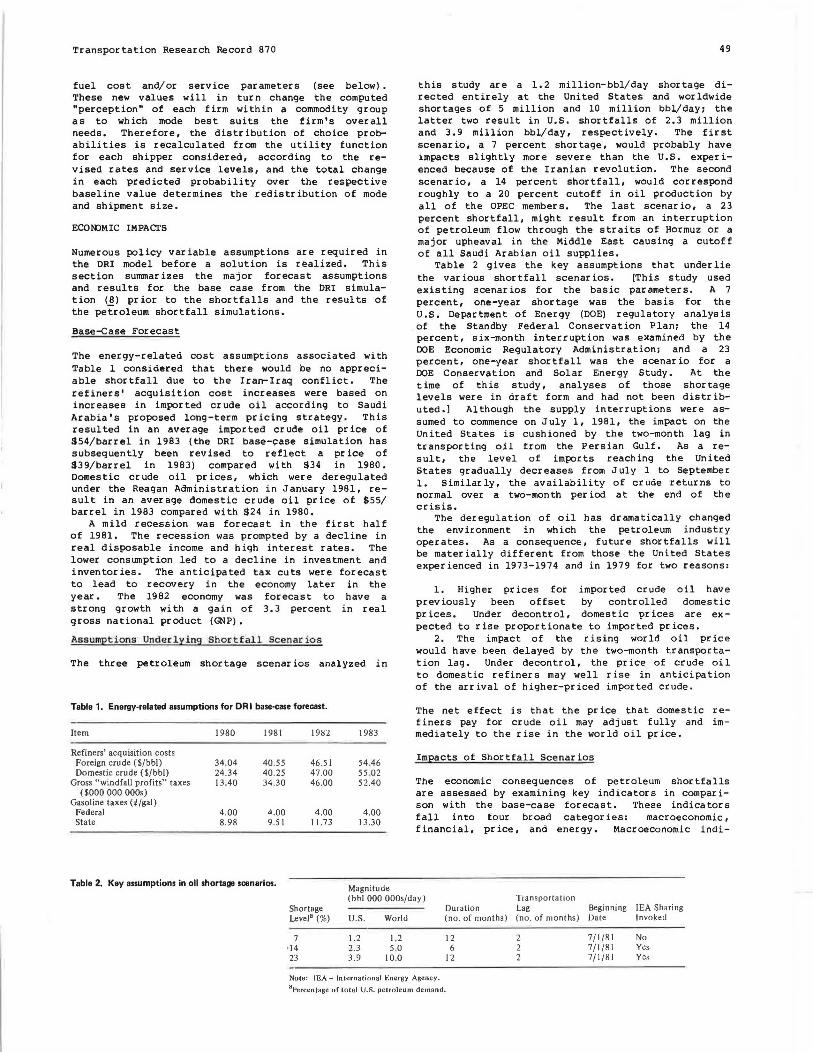
The energy-related cost assumptions associated with Table l considered that there would be no appreci­able shortfall due to the Iran-Iraq conflict. The refiners' acquisition cost increases were based on increases in imported crude oil according to Saudi Arabia's proposed long-term pricing strategy. This resulted in an aver age imported er ude oil pr ice of S54/barrel in 1983 (the DRI base-case simulation has subsequently been revised to reflect a price of S39/barrel in 1983) compared with S34 in 1980, Domestic crude oil prices, which were deregulated under the Reagan Administration in January 1981, re­sult in an average domestic crude oil price of $55/ barrel in 1983 compared with S24 in 1980.

A mild recession was forecast in the first half of 1981. The recession was prompted by a decline in real disposable income and high interest rates. The lower consumption led to a decline in investment and inventories. The anticipated tax cu ts were forecast to lead to recovery in the economy later in the year. The 1982 economy was forecast to have a strong growth with a gain of 3. 3 percent in real gross national product (GNP).

As sumpt i ons Underlying Short f all Scenacios

The three petroleum shortage scenarios analyzed in

Table 1. Energy-related assumptions for ORI base-case forecast.

Item 1980 1981 1982 1983

Refiners' acquisition costs Foreign crude ($/bbl) 34.04 40.55 46.51 54.46 Domestic crude ($/bbl) 24.34 40.25 47.00 55 .02

Gross "windfall profits" taxes 13.40 34.30 46.00 52.40 ( $000 000 OOOs)

Gasoline taxes (¢/gal) Federal 4.00 4.00 4.00 4.00 State 8.98 9.51 11.73 13.30

Table 2. Key assumptions in oil shortage scenarios. Magnitude

49

this study are a 1.2 million-bbl/day shortage di­rected entirely at the United States and worldwide shortages of 5 million and 10 million bbl/dayi the latter two result in U.S. shortfalls of 2.3 million and 3,9 million bbl/day, respectively. The first scenario, a 7 percent shortage, would probably have impacts slightly more severe than the u.s. experi­enced because of the Iranian revolution. The second scenario, a 14 percent shortfall, would correspond roughly to a 20 percent cutoff in oil production by all of the OPEC members. The last scenario, a 23 percent shortfall, might result from an interruption of petroleum flow through the straits of Hormuz or a major upheaval in the Middle East causing a cutoff of all Saudi Arabian oil supplies.

Table 2 gives the key assumptions that under lie the various shortfall scenarios. [This study used existing scenarios for the basic parameters. A 7 percent, one-year shortage was the basis for the U.S. Department of Energy (DOE) regulatory analysis of the Standby Federal Conservation Plan: the 14 percent, six-month interruption was examined by the DOE Economic Regulatory Administration: and a 23 percent, one-year shortfall was the scenario for a DOE Conservation and Solar Energy Study. At the time of this study, analyses of those shortage levels were in draft form and had not been distrib­uted.] Although the supply interruptions were as­sumed to commence on July l, 1981, the impact on the United States is cushioned by the two-month lag in transporting oil from the Persian Gulf. As a re­sult, the level of imports reaching the United States gradually decreases from July l to September l. Similarly, the availability of crude returns to normal over a two-month period at the end of the crisis.

The deregulation of oil has dramatically changed the environment in which the petroleum industry operates. As a consequence, future shortfalls will be materially different from those the United States experienced in 1973-1974 and in 1979 for two reasons :

l. Higher prices for imported crude oil have previously been offset by controlled domestic prices. Under decontrol, domestic prices are ex­pected to rise proportionate to imported prices.

2. The impact of the rising world oil price would have been delayed by the two-month transporta­tion lag. Under decontrol, the price of crude oil to domestic refiners may well rise in anticipation of the arrival of higher-priced imported crude.

The net effect is that the price that domestic re­finers pay for crude oil may adjust fully and im­mediately to the rise i n the world oil price.

Impacts of Shortfall Scenarios

The economic consequences of petroleum shortfalls are assessed by examin i ng key indicators in compari­son with the base-case forecast. These indicators fall into four broad categories: macroeconomic, financial, pr ice, and energy. Macroeconomic indi-

(bbl 000 OOOs/day) Transportation Shortage Level"(%)

7 •14 23

U.S.

1.2 2.3 3.9

World

1.2 5.0

10.0

Duration (no . of months)

12 6

12

Note: IEA = International Energy Agency. 8 Percentage of total U.S. petroleum demand.

Lag Beginning IEA Sharing (no. of months) Date Invoked

2 7/ I /81 No 2 7/ I /81 Yes 2 7/1/81 Yes

:::l '

50

ca tors include real GNP, housing star ts, automobile sales, and unemployment. Financial indicators in­clude the federal deficit, the federal funds rate, and the prime rate. Price indicators include the producer pr ice index, the consumer pr ice index, and core inflation. Energy indicators include the pr ices of gasoline and home heating oil and total gasoline consumption. These indicators were ex­amined as to their immediate and long-run behavior due to future petroleum shortfalls compared with the base case and 1979 shortfall. Real GNP, gasoline prices, and total gasoline consumption effects dur­ing the petroleum shortfalls are discussed here in further detail.

Real GNP

The base case for GNP forecast shows a mild reces­sion in the first half of 1981 followed by a moder­ate recovery through the balance of the forecast period. The impact of a 7 percent oil shortage on GNP is expected to be relatively minor. GNP is off about 1 percent; by the end of 1983, the economy is about one-quarter behind the base-case forecast. Despite its short 6-month duration, the 14 percent shortfall scenario could be expected to deprive the economy of 12 months of growth. Real GNP recovers from the third quarter of 1982, although it would continue to lag about a year behind the base case, so that GNP would be down nearly 3 percent by the end of 1983. The greater magnitude and duration of the 23 percent shortfall leads to four quarters of declining real GNP followed by a very weak to moder­ate recovery in 1983. It should be noted that by the last quarter of 1983 the economy would have lost almost two years of growth and be more than 5 per­cent behind the base case.

The impacts of a severe petroleum shortfall are twofold:

1. The economy loses one to two years of real growth.

2. Output that is lost during several years of weaker economic growth will not be recovered. Fu­ture economic growth starts from a lower base and continues to lag behind the control forecast.

Price of Gasoline

The pr ice of gasoline over the past decade has in­creased gradually with the exception of two rapid upward movements (1973-1974 and 1979), both caused by imported petroleum supply interruptions. Depend­ing on storage supplies and the state of the econ­omy, future interruptions could cause a similar price spurt. In fact, the absence of price regula­tions could cause the price adjustment to be quicker and more severe than in previous crises. In con­trast, though, current high inventories of petroleum and refined products, as well as the fuel switching capability (from oil to gas) in some industries, provide a cushion against the upward price pressures caused by an oil shortage.

The control forecast is predicated on the absence of further oil price shocks during the forecast pe­riod and gasoline prices drifting upward at 1-2 .C/month, breaking the S2 level in the last half ot 1983 (th is reflects pr ice increases of 15-20 per­cent/year over the forecast period).

The shortfall prices, referenced here and based on the DRI model, are not equilibrium prices but rather retail prices that reflect the higher crude oil acquisition costs and production and distribu­tion costs. More will be said later in this paper about equilibrium prices, but the general trend of the curves is likely to be the same. In the 7 per-

Transportation Research Record 870

cent case, the major adjustment occurs by mid-1982, when the pr ice of gasoline exceeds $2/gal. In the following quarters, the price of gasoline resumes a steady upward climb. In the 14 percent scenario, pr ices would adjust over a four-quarter period to reflect the new, higher crude prices: After reach­ing S2.63 in the second quarter of 1982, prices drift downward through the end of the year before rising again in 1983. In the 23 percent scenario, prices would adjust over a six-quarter period, breaking the 84 level in the last half of 1982. However, this price level is not sustainable, and a downward correction of more than 15 percent is fore­cast for 1983.

A doubling of gasoline prices over the course of a single year would be significant. However, more significant is the fact that a crisis-induced gas­oline price level, after a relatively minor adjust­ment, sets the floor for future gasoline prices. Following the 1979 crisis, the price of gasoline nearly doubled; in the ensuing glut of gasoline in­ventories, however, the pr ice has displayed remark­able resiliency. The shortfall scenarios suggest that, once again, the market would adjust to a per­manently higher gasoline price level.

Beyond the aggregate economic impacts discussed above, a major, permanent increase in petroleum product prices has implications for key sectors and a number of regions. The automobile and housing industries are severely affected. Production in the steel industry, which supplies both, would be off 10 percent during 1982 and 1983 in the 23 percent shortage case compared with the base case. Chemi­cals, nonferrous metals, stone, clay, and glass all suffer 10-15 percent losses in output.

On a regional level, a shortage would most di­rectly affect the industrial Midwest and Northeast, where a large fr action of heavy industry is lo­cated. In the short run, tourist reg ions and indus­tries would be benefited by gasoline availability; in the long run, they would be hurt by its continued higher price. This long-run effect reflects a shift in consumer buying patterns from energy-intensive goods and activities.

Total Gasoline Consumption

Total gasoline consumption is a broad indicator of the price sensitivity of gasoline demand. The con­trol forecast predicts a slow downward drift in con­sumption over the 1981-1983 period. This trend is accelerated by a petroleum shortfall. The decline in gasoline consumption is disproportionately large in comparison with the crude oil shortfall during the shortage. This reflects attempts to meet dis­tillate demands at the expense of discretionary uses of gasoline such as pleasure driving.

Summary

The base-case forecast period presumes an economic recovery in this analysis. For that reason, the shortage impacts are tempered by the existing ex­pansionary forces in the economy. The 7 percent, and even the 14 percent, shortages still allow for over all economic growth in spite of severe effects in some sectors. The 23 percent shortage produces a recession. The major short-run impacts of any of the oil shortage scenarios include a reduction in GNP, increases in prices and interest rates, and a reduction in petroleum product supply, which drives pr ices up. Automobile sales and housing construc­t ion are the two sectors most severely affected.

The longer-term consequences of petroleum supply interruptions include GNP growth from a lower base, inflation at a higher rate, and higher petroleum

Transportation Research Record 870

product prices long after the shortage has ended.

SHORTFALL-INDUCED CHANGES IN FREIGHT TRANSPORTATION

The effects of interruptions in the petroleum supply on freight transportation demand are manifested in two distinct ways:

1. The resulting decline in economic activity will mean less demand for freight to be transported and therefore less fuel consumed. These changes in economic activity are not uniform across all sec­tors; thus, the various transportation modes are affected differently.

2. Apart from the shortfall-induced economic decline, a rapid increase in the price of fuel can be expected in the absence of pr ice controls; this would result in a further decline in the demand for freight transportation and produce shifts in the modal choice of shippers. (An area for further analysis is the cyclic effect of increasing trans­portation prices on economic activity in the various commodity sectors, which is beyond the scope of this study.) Furthermore, the extent of the decline in total economic activity is not the same as the mag­nitude of a petroleum shortfall, since each industry varies as to its dependence on petroleum. As a con­sequence, transportation firms face the prospect of a relatively high demand for their services forcing them to seek new sources of fuel supply, increase their conservation efforts, or most likely a combi­nation of both.

Transportation Activity in Base Case

Forecast changes in the economic activity of some individual sectors have significant influence on several of the freight modes. Mining and construc­tion industries are good examples of changing TMT activity as calculated by FRATE. In the base case, the coal-mining sector was forecast to have declin­ing output in 1981 due to an anticipated miners' strike. In 1982 and 1983, the industry was forecast to recover and grow at a rate double the GNP rate. This is of special significance to the railroads, some of which depend on coal as their chief revenue source. The construction industry is expected to gear up for new housing starts by 1981. It is at this point that the industry would be experiencing the most rapid growth rate since 1977. Since the trucking industry dominates transportation in the construction sector, it is expected to benefit con­siderably from this growth.

The TMT projection for oil and gas shows growth at 1.6 percent annually, only half the rate of GNP. Movements of petroleum products are expected to gradually decline due to the continued conserva­tion. This decreased demand will particularly af­fect pipeline and waterway operators.

Increases in industrial products are prompted by a strong recovery in business investments in 1982 and 1983. This suggests that the ton miles for high-valued, time-sensitive manufactured goods that travel by truck and air will increase.

Overall, the base-case growth areas are those that are dominated by truck travel. By 1983, nearly all of the manufacturing sectors are growing faster than GNP. Primary products that are carried by rail show a steady but slower growth rate.

Transportation Activity in Shortfall Scenarios

The freight transportation industry is affected in several distinct ways during an interruption in the petroleum supply. First, shippers make transporta-

51

tion decisions due to changes in output as a result of the shortfall and fuel price increases. In addi­tion, carriers may initiate operational changes to save fuel. Only the influence of shipper decisions is examined here; evaluations of operational changes that carriers can use to reduce their demand for fuel were not available at the time this paper was written.

Effects of Changes in Economic Activity on Freight Transportation

The relation between economic indicators and freight transportation during an energy shortfall may be different from the historical association of GNP and intercity TMT, since freight movement tends to be a lagging indicator of economic activity. When less petroleum is supplied to a national economy than is anticipated, a decline in economic activity will occur regardless of whether the prices of crude oil and refined petroleum products are controlled or not. The change in economic activity, which will vary widely by industry sector, will then directly affect freight transportation in that fewer goods will be transported. To the extent that the demand for freight transportation declines, the demand for transportation fuel will also decline, assuming no shift to energy-intensive modes for the remaining traffic.

To illustrate the effects of a petroleum short­fall in some detail, the analysis focuses on a par­ticular quarter during the supply interruption rather than presenting an overview of the quarter­to-quarter changes. The first quarter of 1982 has been selected, since it embodies the cumulative results of nearly two quarters of the effects of the various petroleum shortfall scenarios (assumed to begin July 1, 1981, although the effect on the United States is cushioned by the two-month lag in transporting oil from the Persian Gulf). By using the DRI changes in sectoral growth rates with the corresponding FRATE sectors, the change in freight transportation demand due to the change in goods output can be isolated. This would be the effect if fuel prices were frozen at the outset of the short­fall. The cor,strained fuel supply, though, indi­cates that this demand situation is far from equi-libr ium.

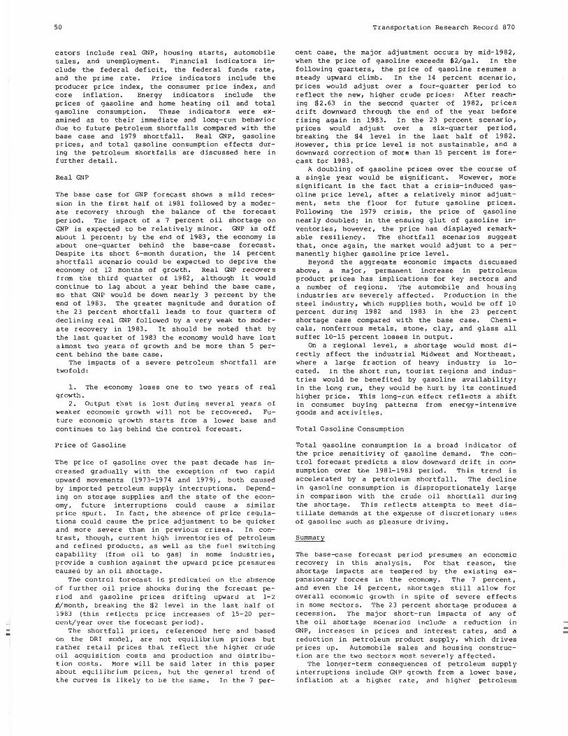
One of the most significant results shown is that the demand for freight transportation has been re­duced by only a small fraction of the extent of the shortfalls. Even in the 23 percent shortfall case, the demand for freight transportation declines only 3.2 percent. The resulting decrease in the demand for fuel is even less--1.6 percent--as given in Table 3.

The combination of several factors produces these changes. The primary goods sectors, which account for about 40 percent of all TMT, experience mixed effects. The mining sectors, due to their highly energy-intensive operations, decline during a petro­leum shortfall. This adversely affects the modes handling these bulk commodities--principally the railroads and marine transportation. Movements of domestic crude oil and natural gas are increased slightly as the result of increased oil and gas pro­duction in response to refiners' higher crude oil acquisition cost during a shortfall. Pipelines benefit from this, although the total TMT for this mode would be down due to decreased volume of re­fined petroleum products. Energy use for pipelines would be increased slightly due to the high energy intensity for natural gas pipelines.

In the manufacturing industries, which require primary goods as input, production is not shown to change as substantially as in the primary sectors,

--

52

Table 3. Change in freight transportation intercity TMT and energy demand due to decline in economic activity: first quarter of 1982.

Change by Shortfall Level ( % )

TMT Energy Use

7 14 23 7 14 23 Mode Percent Percent Percent Percent Percent Percent

Truck -1.2 -1.6 -2.0 -1.2 -1.6 -2.0 Rail -1.6 -2.0 -2.4 -1.8 -2.3 -2.6 Water -1.9 -3.0 -4.7 -1.6 -2.5 -4.0 Air -0.6 -0.8 -1.0 -2.0 -2.4 -2.8 Pipeline -1.2 -1.9 -3.4 +O.l +0.4 +0.7

Avg -1.5 -2 .2 -3.2 -1.0 -1.2 -1.6

especially in the initial periods of an energy shortfall, Stockpiling of production inputs is com­mon among manufacturers, Inventories above normal operational requirements ensure that production goals can be met, even in the face of extended transportation difficulties, such as prolonged transportation worker strikes or adverse weather conditions. A major exception to this generaliza­tion about manufacturing industries is the motor­vehicle sector, which is the sector most seriously affected during an interruption in petroleum sup­ply. Generally, the relatively mild effects for much ot the manufacturing sectors would keep the demand for the truck mode relatively high.

This change in the demand for freight transpor­tation as influenced by declining economic activity could only be expected to occur if the pr ice of transportation fuels were frozen at the preshortfall levels. Although this would not be expected to happen, the isolation of this component of freight transportation demand provides a useful basis for examining, in perspective, the fuel pr ice effects on the freight transportation industry.

Fuel Price Effects on Freight Transportation

As shown in the previous section, the decline in economic activity is not nearly as large as the de­cline in the availability of transportation fuels during a petroleum shortfall, The purpose of that section was to illustrate the economic activity com­ponent of the change in freight transportation de­mand. Since shipping decisions are significantly influenced by freight rates, fuel pr ices could be expected to have a considerable impact on the amount and modal distribution of goods movement.

By again using the first quarter of 1982 as the analysis period, the NAFDEM model was used to iter­ate to an equilibrium fuel price--one that produces changes in shipnent size, mode shifts, or reductions in the volumes shipped to the extent that fuel de­mand approximates that available during the short­fall.

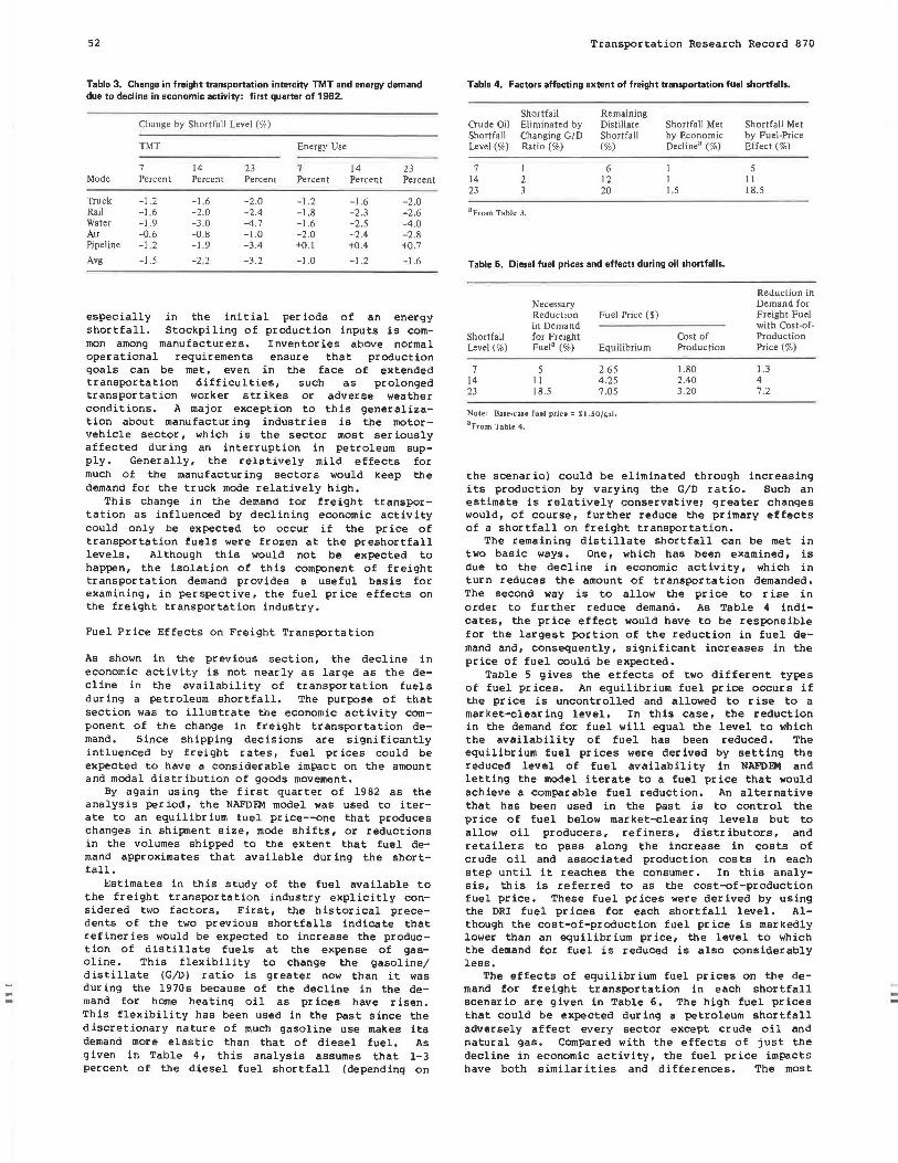
Estimates in this study of the fuel available to the freight transportation industry explicitly con­sidered two factors. First, the historical prece­dents of the two previous shortfalls indicate that refineries would be expected to increase the produc­tion of distillate fuels at the expense of gas­oline. This flexibility to change the gasoline/ distillate (G/D) ratio is greater now than it was during the 1970s because of the decline in the de­mand for home heating oil as prices have risen. This flexibility has been used in the past since the discretionary nature of much gasoline use makes its demand more elastic than that of diesel fuel. As given in Table 4, this analysis assumes that 1-3 percent of the diesel fuel shortfall (depending on

Transportation Research Record 670

Table 4. Factors affecting extent of freight transportation fuel shortfalls.

Shortfall Remaining Crude Oil Eliminated by Distillate Shortfall Met Shortfall Changing G/D Shortfall by Economic Level(%) Ratio(%) (%) Decline• (%)

7 I 6 l 14 2 12 I 23 3 20 l.5

aFrom Table 3.

Table 5. Diesel fuel prices and effects during oil shortfalls.

Necessary Reduction Fuel Price($) in Demand

Shortfall for Freight Level(%) Fuel" (%) Equilibrium

7 5 2.65 14 II 4.25 23 18.5 7.05

Nole: Base-case fuel pric111 :: $ I.SO/g:a.1. 8 From Table 4.

Cost of Production

1.80 2.40 3.20

Shortfall Met by Fuel-Price Effect(%)

5 11 18.5

Reduction in Demand for Freight Fuel with Cost-of­Production Price(%)

1.3 4 7.2

the scenario) could be eliminated through increasing its production by varying the G/D ratio. Such an estimate is relatively conservativei greater changes would, of course, further reduce the primary effects of a shortfall on freight transportation.

The remaining distillate shortfall can be met in two basic ways. One, which has been examined, is due to the decline in economic activity, which in turn reduces the amount of transportation demanded. The second way is to allow the pr ice to rise in order to further reduce demand. As Table 4 indi­cates, the price effect would have to be responsible for the largest portion of the reduction in fuel de­mand and, consequently, significant increases in the price of fuel could be expected.

Table 5 gives the effects of two different types of fuel prices. An equilibrium fuel price occurs if the price is uncontrolled and allowed to rise to a market-clearing level. In this case, the reduction in the demand for fuel will equal the level to which the availability of fuel has been reduced. The equilibrium fuel prices were derived by setting the reduced level of fuel availability in NAFDEM and letting the model iterate to a fuel price that would achieve a comparable fuel reduction. An alternative that has been used in the past is to control the pr ice of fuel below market-clearing levels but to allow oil producers, refiners, distributors, and retailers to pass along the increase in costs of crude oil and associated production costs in each step until it reaches the consumer. In this analy­sis, this is referred to as the cost-of-production fuel price. These fuel prices were derived by using the ORI fuel pr ices for each shortfall level. Al­though the cost-of-production fuel price is markedly lower than an equilibrium price, the level to which the demand for fuel is reduced is also considerably less.

The effects of equilibrium fuel prices on the de­mand for freight transportation in each shortfall scenario are given in Table 6. The high fuel prices that could be expected during a petroleum shortfall adversely affect every sector except crude oil and natural gas. Compared with the effects of just the decline in economic activity, the fuel price impacts have both similarities and differences. The most

Transportation Research Record 870

Table 6. Change in freight transportation TMT and energy demand due to equilibrium fuel prices: first quarlllr of 1982.

Change by Shortfall Level (%)

TMT Energy Use

7 14 23 7 14 23 Mode Percent Percent Percent Percent Percent Percent

Truck -6.0 -12.8 -21.8 -6.9 -13.6 -22.6 Rail -4.5 -10.7 -18.5 -5.4 -11.5 -19.4 Water -0.6 -1.0 -1.5 -0.8 -1.5 -2.2 Air -2.7 -8.2 -15.6 -3.8 -9.2 -16.7

Avg• -3.5 -7.8 -13.3 -5.4 -11.2 -18.9

8 Excludes pipeline.

Table 7. Modal shares of tons and'ton miles of freight transportation during oil shortfalls: first quarter of 1982.

Modal Share by Shortfall Level(%)

Tons Ton Miles

0 7 14 23 0 7 14 23 Per- Per- Per· Per- Per- Per- Per- Per-

Mode cent8 cent cent cent cent cent cent cent

Truck 35.l 34.5 33.7 32.7 26.2 25.7 25.0 24.0 Rail 49.4 49.8 50.3 51.0 37.3 36.8 36.l 35.2 Water 12.8 13.0 13.2 13.5 36.3 37.3 38.7 40.6 Air 2.7 2.7 2.8 2.8 0.2 0.2 0.2 0.2 Totalb 100.0 100.0 100.0 100.0 100.0 100.0 100.0 100.0

8 Base case. bExcludes pipelines.

obvious difference is the degree of influence on the demand for freight transportation. It is within the commodity sectors, though, that some important ob­servations can be made. The primary goods indus­tries that dominate bulk goods shipments continue to show significant reductions in freight transporta­tion demand. The manufacturing sectors, which pre­viously had indicated a relatively small decline in economic activity, are now shown to be sensitive to shipping costs. As a result, the truck mode begins to reflect a greater share in the loss of freight shipping demand because of the loss of traffic in those sectors in which it is the predominant car­rier. In contrast to the economic activity compo­nent of freight transportation demand, increases in fuel prices produce modal shifts in favor of the rail and water modes.

Changes in freight transportation demand in re­sponse to a partially controlled fuel price, such as the cost-of-production pr ice, are in the same di­rection as shown for the equilibrium pr ice, but the magnitude, as expected, is less.

Changes in Modal Preference

The total tons to be shipped declines, as expected, during an oil shortfall. In the case of equilibrium fuel prices, total tons shipped are forecast to de­cline 5 .6, 12, and 20. 5 percent for the 7, 14, and 23 percent shortfalls, respectively. Since fuel prices are an important component of operating costs for the carriers, freight rates would change as fuel prices increase. This, in turn, would cause ship­pers to modify their total shipments or choice of mode in order to minimize transportation costs. Table 7 gives the changes in the mode share of tons shipped and ton miles as a result of the change in fuel pr ice (equilibrium level) along with the de­cline in economic activity. Although it is not shown in the table, tons shipped and ton miles of

53

travel decline not only in the aggregate but also for each mode. Therefore, even though dramatic mode shifts do not appear, freight traffic within mode will decrease.

Pipelines were excluded from this analysis since they carry only crude oil, natural gas, and refined petroleum products. As mentioned ear lier, the do­mestic movements in the first two sectors increase slightly during an interruption in the oil supply. Pipelines, generally recognized as the most effi­cient freight mode, would be the beneficiary. As the principal mover of refined petroleum products, pipelines would show a decline in traffic in this sector. Overall, the specialized nature of pipe­lines would mean that this mode is excluded from the decisions of shippers in most commodity sectors. Thus, the analysis was directed to the remaining four modes.

Air

The air freight mode is the most energy intensive of the competitive modes. It provides a service for those shippers whose commodities are time sensi­tive. Even without petroleum supply problems, ship­pers pay a premium price to use this mode. Conse­quently, it is not unexpected that the demand for this mode is relatively inelastic. The tons shipped by air decline, though to a lesser extent than for the other modes; as a result, its market share of freight transportation demand remains relatively constant, whether expressed in tons shipped or ton miles of travel. Some shift to the truck mode, which generally has the next-highest service char­acter is tics, would be expected. Even with a con­stant or slightly increasing market share, air freight would still account for a very small per­centa9e of total freight transportation energy demand.

Tntck

The truck mode, under equilibrium fuel-price condi­tions, was forecast to have the largest decline in freight traffic. In terms of tons shipped, the truck share declines from 35 .1 percent in the base case to 32. 7 percent in the 23 percent shortfall case. Given the !17/gal fuel price that was fore­cast, a greater shift away from this mode might be anticipated, Several factors, thouqh, limit the potential shift from truck to other modes. First, the truck (highway) network is considerably more extensive than the networks for the competing modes, which restricts the opportunity for modal choice for many origin-destination routes. Many of the shorter intercity trips would continue to use trucks. Less­than-truckload (LTL) shipments would probably be consolidated into truckload shipments before a modal shift would occur. In addition, the fraction of operating expenses for the truck mode that fuel rep­resents is not vastly different than it is for the truck mode's chief competitor, the rail mode. As a result, the changes in freight rates are not likely to be substantial. In fact, for LTL operations, the percentage of operating costs attributed to fuel is about half of what it is for truckload operations. But some shift of truck traffic to the rail mode would be expected.

Rail

Although rail freight traffic does decline just as with the other modes, the market share increases. This situation, which occurs with an equilibrium fuel price, is in contrast to the change due only to the decline in economic activity without any in-

--

54

crease in fuel prices. In that situation, the de­crease in the demand for freight transportation is greater for rail than for truck. With an equilib­r ium fuel price, rail improves its market share. The shift to increased shipment size favors the rail­road, and it is likely that rail will increase its share of intermodal traffic for longer-haul trips in those corridors where rail can provide dedicated service. Equipment availability may become a limit­ing factor. Even though railroads may gain traffic at the expense of the truck mode, rail may lose some traffic to water transportation where that mode is available.

Water

The total demand for marine transportation is also down during a petroleum shortfall, although its rel­ative energy efficiency makes it extremely competi­tive for bulk shipments during a time of rising fuel prices. This is true even though fuel is a very high percentage of operating costs for this mode. The model showed that the water modal share of both tons shipped and TMT would increase during any of the shortfalls tested. In corridors where this mode is competitive, it could be anticipated that some rail traffic will shift to marine transportation.

CONCLUSIONS

A pattern has begun to emerge from the effects of various fuel price levels. If prices are frozen at preshortfall levels, the changes in economic activ­ity will affect the primary goods sectors the most. Rail and water transportation would see the greatest decline in the demand for their services. The de­mand for fuel, however, will continue to exceed by far the available supply. If fuel pr ices are al­lowed to rise to an equilibrium level, then the de­mand for fuel will be balanced with the reduced sup­plies. Total traffic will be decreased, and shifts in modal preference will generally be in the direc­tion of air to truck, truck to rail, and rail to water.

From a policy perspective, there is often discus­sion of allocating fuel to those modes considered more energy efficient than others. This analysis shows that shifts in modal preference would tend to occur in the direction that an allocation program would probably try to achieve. In addition, allow­ing fuel prices to rise to an equilibrium level pro­vides incentives for carriers and shippers to con­serve energy by minimizing costs.

As noted in the analysis, a fuel pr ice that is controlled below an equilibrium level will result in a gap between the demand for and the supply of fuel. In the past, this has introduced considerable uncertainty into the marketplace. In contrast to fuel supplies actually being available (al though at high pr ices in an equilibrium case), fuel was per-

Transportation Research Record 870

ceived to be available when it was not. This was most evident at the retail level of the truckstops, which tended to be the weakest link in the distil­late fuel distribution chain. For the truck mode, in particular, this perception by carriers could re­sult in a significant decrease in the reliability of delivery schedules. Spot shortages also were re­ported for the other modes, especially marine trans­portation. However, the problems were generally less severe for the bulk fuel purchasers. Although fuel distribution problems could be expected in the initial stage of an oil shortfall even under equi­librium pr1c1ng conditions, the adjustment period would probably be much shorter than it would with controlled prices.

ACKNOWLEDGMENT

This paper was developed from a project sponsored by DOE. Numerous people have been extremely helpful in the progress of the study. Georgia Johnson, the DOE project manager, provided invaluable assistance and guidance throughout the project. Arvind Teotia and Yehuda Klein from Argonne National Laboratory con­tributed much to the economic analysis phase of the project. Ian Harrington and Fred Manner ing from the Massachusetts Institute of Technology were responsi­ble for the development of one of the models used in the analysis. Many others provided useful insights and review throughout the study.

REFERENCES

1. Commodity Transportation Survey. U.S. Bureau of the Census, TC72C2-8, 1972.

2. U.S. Long-Term Review. Data Resources, Inc., Washington, DC, Jan. 1981,

3. M.S. Bronzini. Freight Transportation Energy Use. Research and Special Programs Bureau, U.S. Department of Transportation, Rept. DOT-TSC-OST-79-1, July 1979.

4. J,R, Wagner. Brookhaven Energy Transportation Submodel (BETS) Documentation and Results. Di­v1s1on of Transportation Energy Conservation, u.s. Department of Energy, Upton, NY, Oct. 1977.

5 . G. Kulp and others. Transportation Energy Con­servation Data Book, 3rd and 4th eds. Oak Ridge National Laboratory, Oak Ridge, TN, 1979, 1980.

6. A. Rose. Energy Intensity and Related Parame­ters of Selected Transportation Modes: Freight Movements. Oak Ridge National Laboratory, Oak Ridge, TN, ORNL/TM-6700, 1979.

7. Y.S. Chiang and others. A Short-Run Freight De­mand Model: The Joint Choice of Mode and Ship­ment Size. Massachusetts Institute of Tech­nology, Cambridge, July 1980,

8. The Data Resources Review of the U.S. Economy. Data Resources, Inc., Washington, DC, Feb. 1981.

--