Monitoring Corruption: Evidence from a Field Experiment in ...
Upload
truongdieuCategory
view
218download
0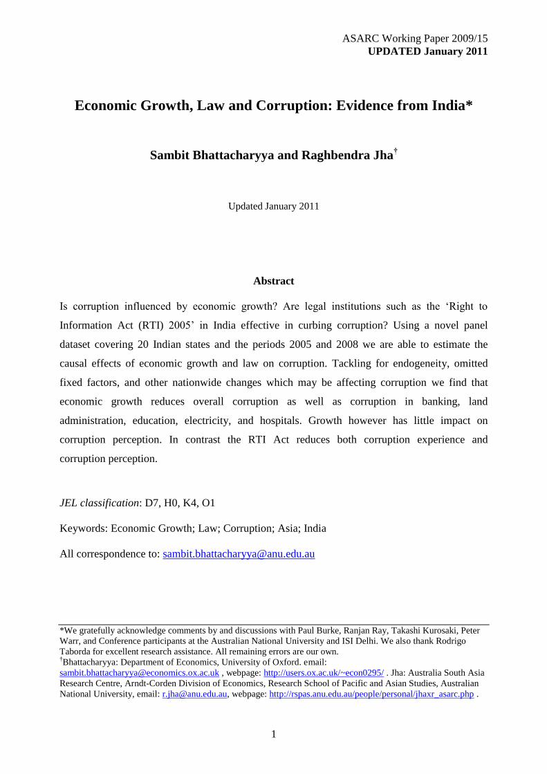
ASARC Working Paper 2009/15
UPDATED January 2011
1
Economic Growth, Law and Corruption: Evidence from India*
Sambit Bhattacharyya and Raghbendra Jha†
Updated January 2011
Abstract
Is corruption influenced by economic growth? Are legal institutions such as the „Right to
Information Act (RTI) 2005‟ in India effective in curbing corruption? Using a novel panel
dataset covering 20 Indian states and the periods 2005 and 2008 we are able to estimate the
causal effects of economic growth and law on corruption. Tackling for endogeneity, omitted
fixed factors, and other nationwide changes which may be affecting corruption we find that
economic growth reduces overall corruption as well as corruption in banking, land
administration, education, electricity, and hospitals. Growth however has little impact on
corruption perception. In contrast the RTI Act reduces both corruption experience and
corruption perception.
JEL classification: D7, H0, K4, O1
Keywords: Economic Growth; Law; Corruption; Asia; India
All correspondence to: [email protected]
*We gratefully acknowledge comments by and discussions with Paul Burke, Ranjan Ray, Takashi Kurosaki, Peter
Warr, and Conference participants at the Australian National University and ISI Delhi. We also thank Rodrigo
Taborda for excellent research assistance. All remaining errors are our own. †Bhattacharyya: Department of Economics, University of Oxford. email:
[email protected] , webpage: http://users.ox.ac.uk/~econ0295/ . Jha: Australia South Asia
Research Centre, Arndt-Corden Division of Economics, Research School of Pacific and Asian Studies, Australian
National University, email: [email protected], webpage: http://rspas.anu.edu.au/people/personal/jhaxr_asarc.php .
Sambit Bhattacharyya and Raghbendra Jha
ASARC WP 2009/15 UPDATED JAN 2011 2
1. Introduction
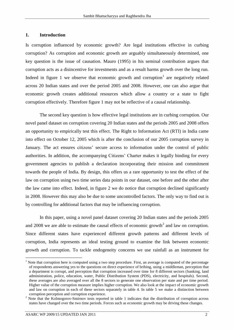
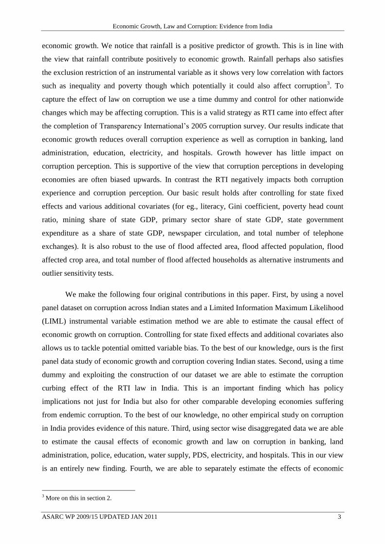
Is corruption influenced by economic growth? Are legal institutions effective in curbing
corruption? As corruption and economic growth are arguably simultaneously determined, one
key question is the issue of causation. Mauro (1995) in his seminal contribution argues that
corruption acts as a disincentive for investments and as a result harms growth over the long run.
Indeed in figure 1 we observe that economic growth and corruption1 are negatively related
across 20 Indian states and over the period 2005 and 2008. However, one can also argue that
economic growth creates additional resources which allow a country or a state to fight
corruption effectively. Therefore figure 1 may not be reflective of a causal relationship.
The second key question is how effective legal institutions are in curbing corruption. Our
novel panel dataset on corruption covering 20 Indian states and the periods 2005 and 2008 offers
an opportunity to empirically test this effect. The Right to Information Act (RTI) in India came
into effect on October 12, 2005 which is after the conclusion of our 2005 corruption survey in
January. The act ensures citizens‟ secure access to information under the control of public
authorities. In addition, the accompanying Citizens‟ Charter makes it legally binding for every
government agencies to publish a declaration incorporating their mission and commitment
towards the people of India. By design, this offers us a rare opportunity to test the effect of the
law on corruption using two time series data points in our dataset, one before and the other after
the law came into effect. Indeed, in figure 2 we do notice that corruption declined significantly
in 2008. However this may also be due to some uncontrolled factors. The only way to find out is
by controlling for additional factors that may be influencing corruption.
In this paper, using a novel panel dataset covering 20 Indian states and the periods 2005
and 2008 we are able to estimate the causal effects of economic growth2 and law on corruption.
Since different states have experienced different growth patterns and different levels of
corruption, India represents an ideal testing ground to examine the link between economic
growth and corruption. To tackle endogeneity concerns we use rainfall as an instrument for
1 Note that corruption here is computed using a two step procedure. First, an average is computed of the percentage
of respondents answering yes to the questions on direct experience of bribing, using a middleman, perception that
a department is corrupt, and perception that corruption increased over time for 8 different sectors (banking, land
administration, police, education, water, Public Distribution System (PDS), electricity, and hospitals). Second,
these averages are also averaged over all the 8 sectors to generate one observation per state and per time period.
Higher value of the corruption measure implies higher corruption. We also look at the impact of economic growth
and law on corruption in each of these sectors separately in table 4. In table 5 we make a distinction between
corruption perception and corruption experience. 2 Note that the Kolmogorov-Smirnov tests reported in table 1 indicates that the distribution of corruption across
states have changed over the two time periods. Forces such as economic growth may be driving these changes.
Economic Growth, Law and Corruption: Evidence from India
ASARC WP 2009/15 UPDATED JAN 2011 3
economic growth. We notice that rainfall is a positive predictor of growth. This is in line with
the view that rainfall contribute positively to economic growth. Rainfall perhaps also satisfies
the exclusion restriction of an instrumental variable as it shows very low correlation with factors
such as inequality and poverty though which potentially it could also affect corruption3. To
capture the effect of law on corruption we use a time dummy and control for other nationwide
changes which may be affecting corruption. This is a valid strategy as RTI came into effect after
the completion of Transparency International‟s 2005 corruption survey. Our results indicate that
economic growth reduces overall corruption experience as well as corruption in banking, land
administration, education, electricity, and hospitals. Growth however has little impact on
corruption perception. This is supportive of the view that corruption perceptions in developing
economies are often biased upwards. In contrast the RTI negatively impacts both corruption
experience and corruption perception. Our basic result holds after controlling for state fixed
effects and various additional covariates (for eg., literacy, Gini coefficient, poverty head count
ratio, mining share of state GDP, primary sector share of state GDP, state government
expenditure as a share of state GDP, newspaper circulation, and total number of telephone
exchanges). It is also robust to the use of flood affected area, flood affected population, flood
affected crop area, and total number of flood affected households as alternative instruments and
outlier sensitivity tests.
We make the following four original contributions in this paper. First, by using a novel
panel dataset on corruption across Indian states and a Limited Information Maximum Likelihood
(LIML) instrumental variable estimation method we are able to estimate the causal effect of
economic growth on corruption. Controlling for state fixed effects and additional covariates also
allows us to tackle potential omitted variable bias. To the best of our knowledge, ours is the first
panel data study of economic growth and corruption covering Indian states. Second, using a time
dummy and exploiting the construction of our dataset we are able to estimate the corruption
curbing effect of the RTI law in India. This is an important finding which has policy
implications not just for India but also for other comparable developing economies suffering
from endemic corruption. To the best of our knowledge, no other empirical study on corruption
in India provides evidence of this nature. Third, using sector wise disaggregated data we are able
to estimate the causal effects of economic growth and law on corruption in banking, land
administration, police, education, water supply, PDS, electricity, and hospitals. This in our view
is an entirely new finding. Fourth, we are able to separately estimate the effects of economic
3 More on this in section 2.
Sambit Bhattacharyya and Raghbendra Jha
ASARC WP 2009/15 UPDATED JAN 2011 4
growth and law on corruption experience and corruption perception and we do find that they are
different. We notice that economic growth has very little influence on corruption perception.
Our finding adds to a small but growing body of evidence on the difference between corruption
perception and corruption experience (see Olken, 2009).
Our economic growth and corruption result is related to a large literature on corruption
and development which follows from the seminal contribution by Mauro (1995).4 However, note
that our focus here is to estimate the causal effect of economic growth on corruption and not the
other way around. Our law and corruption result is also related to a growing literature on
democratization and corruption as it emphasizes the role of accountability. For example,
Treisman (2000) show that a long exposure to democracy reduces corruption. Bhattacharyya and
Hodler (2010) using a game theoretical model and cross-national panel data estimation of a
reduced form econometric model show that resource rent is bad for corruption however the
effect is moderated by strong democratic institutions. In contrast, Fan et al. (2009) show that
decentralized government may not increase accountability and reduce corruption if the
government structures are complex. In a similar vein, Olken (2007) also show that top down
government audit works better than grassroots monitoring in Indonesia‟s village roads project.
Therefore, our results contribute to a policy debate which is not only important for India but also
for other comparable developing economies. The estimates however are not directly comparable
as there are significant differences in scale (microeconomic or macroeconomic), scope (national
or international), and nature (theoretical, empirical or experimental) of these studies.
Finally, our results are also related to a large literature on institutions and economic
development (see Knack and Keefer, 1995; Hall and Jones, 1999; Acemolgu et al., 2001; Rodrik
et al., 2004; Bhattacharyya, 2009). The major finding of this literature is that economic
institutions (for eg, property rights, contracts, regulation, and corruption) are one of the major
drivers of long run economic development. Besley and Burgess (2000, 2004) provide evidence
that land property rights and labor market institutions have significant effects on economic
performance across states in India. In this paper we estimate the magnitude of the relationship
when causality runs in the opposite direction from economic growth to institutions.
The remainder of the paper is structured as follows: Section 2 discusses empirical
strategy and the data. Section 3 presents the empirical evidence and various robustness tests.
Section 4 concludes.
4Ades and Di Tella (1999), Rose-Ackerman (1999), Dabla-Norris (2000), Leite and Weidmann (2002) are other
important contributions in this literature. Bardhan (1997) provides an excellent survey of the early contributions.

Economic Growth, Law and Corruption: Evidence from India
ASARC WP 2009/15 UPDATED JAN 2011 5
2. Empirical Strategy and Data
We use a panel dataset covering 20 Indian states and the periods 2005 and 2008. Our basic
specification uses corruption data for the periods 2005 and 2008. Economic growth for the
periods 2005 and 2008 are growth in GDP5 over the periods 2004-2005 and 2007-2008
respectively. To estimate the causal effects of economic growth and law on corruption we use
the following model:
1ˆ
it i t it itc y itX (1)
where itc is a measure of corruption in state i at year t , i is a state dummy variable covering
20 Indian states to control for state fixed effects, t is a dummy variable which takes the value 1
for the year 2008 to estimate the impact of the introduction of the RTI Act in October 12 2005,
ˆity is economic growth in state i over the period 1t to t , and itX is a vector of other control
variables. A high value of itc implies a high level of corruption. The motivation behind
including state fixed effects is to control for time invariant state specific fixed factors such as
language, culture, and ethnic fractionalization.
The main variables of interest are ˆity and the time dummy variable t . Therefore 1 and
are our focus parameters. In theory, we would expect 1 to be significantly negative as faster
growing states are able to use additional resources to curb corruption. The coefficient estimate
is expected to be capturing the effect of the RTI Act. This is equivalent to a before and after
estimation strategy in panel data econometrics. Ideally one would like to compare the effect of
RTI on corruption before and afterwards in the areas affected by the law, and then compare this
to the effects before and afterwards in the areas not affected by the law. Unfortunately this is
not feasible here as the RTI law came into effect nationally. In other words, there is no
comparison group here since the law happened at the same time in all locations. Nevertheless,
the strategy implemented here is credible at the macro level.
To illustrate the before and after strategy, let 1itc be the corruption outcome in state i at
time t when the RTI Act is in effect. Similarly, let 2 1itc be the corruption outcome in state i at
time 1t when the RTI Act is not in effect. Note that these are potential outcomes and in
practice we only get to observe one or the other. One can express the above as:
1ˆ[ | , 1, , ]it it iE c i t y y
itX X and 2 1
ˆ[ | , 1 0, , ]it it iE c i t y y it
X X (2)
5 Note that we also use GDP per capita growth rate in table 3 and our results are robust.

Sambit Bhattacharyya and Raghbendra Jha
ASARC WP 2009/15 UPDATED JAN 2011 6
Given that ( | , ) 0itE i t . The population before and after estimates yields the causal
effect of the RTI Act as follows:
1 2 1ˆ ˆ[ | , 1, , ] [ | , 1 0, , ]it it it itE c i t y y E c i t y y
it it
X X X X (3)
This can be estimated by using the sample analog of the population means. If the RTI
law is effective in curbing corruption then we would expect to be negative.
Data on corruption is from the Transparency International‟s India Corruption Study 2005
and 2008. The study was jointly conducted by Transparency International India and the Centre
for Media Studies both located in New Delhi. The survey for the 2005 report was conducted
between December 2004 and January 2005 and the survey for the 2008 report was conducted
between November 2007 and January 2008. The survey asks respondents whether they have
direct experience of bribing, whether they have used a middleman, whether they perceive a
department to be corrupt, and whether they perceive corruption have increased over time.6 These
questions are asked to on average 750 respondents from each of the 20 state. Respondents are
selected using a random sampling technique covering both rural and urban areas. In aggregate
the 2005 survey interviews 14,405 respondents spread over 151 cities, 306 villages of the 20
states. In contrast the 2008 survey covers 22,728 randomly selected Below Poverty Line (BPL)
respondents across the country. One could argue that this brings in issues of measurement error
which will bias our estimates. The bias however is expected to work in the opposite direction as
it will push coefficient estimates downwards. In particular, BPL households are likely to face
more corruption which will lead to over reporting and a positive measurement error. In that case
our coefficient estimates will be biased downwards. This is formally known as attenuation bias.
So what we estimate in the presence of measurement error is in fact less in magnitude than the
true effect. Furthermore, if the measurement error follows all classical assumptions (in other
words, random) then our estimates will remain unaffected. Nevertheless, we use the instrumental
variable (IV) strategy to mitigate measurement error concerns.
Our aggregate measure of corruption itc is computed using the following two steps.
First, an average is computed of the percentage of respondents answering yes to the questions
that they have direct experience of bribing, using a middleman, perception that a department is
corrupt, and perception that corruption increased over time for 8 different sectors (banking, land
administration, police, education, water, Public Distribution System (PDS), electricity, and
6 Note that the survey asks some additional questions. However they are not common over the two time periods in
our study. Therefore we are not including them here.

Economic Growth, Law and Corruption: Evidence from India
ASARC WP 2009/15 UPDATED JAN 2011 7
hospitals).7 Second, these averages are also averaged over all the 8 sectors to generate one
observation per state and per time period. Ideally, one should weight the sectors with their
respective usages. But in the absence of reliable usage statistics at the state level, we compute
averages with equal weights. This may not be a cause for concern as services from all of these
sectors are widely used by citizens. Note that sector level disaggregated data is utilized in table 4
and table 5 treats corruption perception and corruption experience separately. Corruption
experience measure is the average of the questions on „direct experience of bribing‟ and „using a
middleman‟. Corruption perception measure is the average of the questions on „perception that a
department is corrupt‟ and „perception that corruption increased over time‟.
The state of Bihar turns out to be the most corrupt in our sample with 59 percent of
respondents reporting corruption in 2005. In contrast Himachal Pradesh is the least corrupt with
only 17 percent of the respondents reporting corruption in 2008. It appears that Police, land
administration, and Public Distribution System (PDS) are amongst the most corrupt sectors in
our dataset. Kerala and Himachal Pradesh come out to be the least corrupt states in most of the
cases. In contrast Bihar, Jammu and Kashmir, Madhya Pradesh, and Rajasthan register high
levels of corruption.
Economic growth ˆity is defined as the growth in real GDP of the states over the periods
2004-2005 and 2007-2008 respectively. We use real GDP instead of real GDP per capita to
compute growth rates because aggregate growth of the economy is more likely to have an
impact on corruption at the macro level than per capita growth. Nevertheless, we also use per
capita GDP growth to estimate the model and our results are robust. Real GDP data and real per
capita GDP data is from the Planning Commission. Our growth variable varies between -4.2
percent in Bihar in 2005 and almost 17 percent in Chhattisgarh in 2005.
As economic growth here is arguably endogenous, one key question is the issue of
reverse causation. Corruption as argued by many including Mauro (1995) may dampen growth
through the investments channel. In that case a simple OLS estimate of our model would be
biased. In order to estimate the causal effect of economic growth on corruption we need to
implement the instrumental variable estimation strategy. In particular, we need to identify an
exogenous variable that is correlated with economic growth but uncorrelated with the error term
it in the model. In other words, this exogenous variable would affect corruption exclusively
7 Note that the India Corruption Study only reports these macro percentages and the underlying micro data is not
reported.

Sambit Bhattacharyya and Raghbendra Jha
ASARC WP 2009/15 UPDATED JAN 2011 8
through the economic growth channel. This is commonly known as the exclusion restriction.
Indeed, finding such a variable is a challenge in itself. But we are fortunate to have log rainfall
( 1ln itRAIN ) from the Compendium of Environmental Statistics published by the Central
Statistical Organization. We notice that 1ln itRAIN is positively related to economic growth and
the relationship is statistically significant (see table 3, panel B). This is in line with the view that
rainfall positively contributes to economic growth. Furthermore, 1ln itRAIN is geography based
and therefore is exogenous. However, rainfall may affect corruption through channels other than
economic growth. Poverty and inequality are such examples. Rainfall may lead to reduction in
poverty, which may in turn lead to a reduction in corruption. Better rainfall and better
agriculture growth may also increase inequality leading to an increase in corruption. In such a
situation the rainfall instrument may not satisfy the exclusion restriction. To eliminate such
possibility, we check the correlation between the rainfall instrument and poverty and inequality.
It turns out to be 0.17 and 0.38 respectively which suggests it is unlikely that rainfall would
affect corruption through poverty and inequality channel. Therefore, it is safe to conclude that
1ln itRAIN can serve as a valid instrument. However, if the relationship between 1ln itRAIN and
ˆity is not strong enough then it may lead to the weak instruments problem. Staiger and Stock
(1997) and Stock and Yogo (2005) show that if the instruments in a regression are only weakly
correlated with the suspected endogenous variables then the estimates are likely to be biased.
Instruments are considered to be weak if the first stage F-statistic is less than Stock-Yogo critical
value. The Limited Information Maximum Likelihood (LIML) Fuller version of the instrumental
variable method is robust to weak instruments. We implement the LIML method to estimate our
model. Moreover, we operate with a relatively small sample of 40 observations and the LIML
estimates are robust to small samples. Therefore the risk of a significantly large bias due to weak
instruments is minor. We also use flood affected area, flood affected population, flood affected
crop area, and total number of flood affected households as additional instruments and our result
survives. However, these are not our preferred estimates because of sample attrition (see table
8).
Finally, another potential concern is about the power of the diagnostic tests with limited
degrees of freedom. LIML estimates adopted here are best suited for this purpose as they have
robust and powerful small sample properties. Nevertheless, we also perform the following two
tests to be certain about the validity of our conclusions. First, we adopt Hendry et al.‟s (2004)
least square dummy variables approach and our results are robust. This method can be
implemented using the following two steps. First step is to estimate the model using LIML and
Economic Growth, Law and Corruption: Evidence from India
ASARC WP 2009/15 UPDATED JAN 2011 9
identify all the statistically insignificant state dummy variables. Then the second step is to re-
estimate the model using LIML but without the statistically insignificant state dummies. The
advantage is that it significantly improves the power of the tests. Second, we estimate the model
without any state dummies and our results are robust. These results are reported in columns 9
and 10 of table 6.
The time dummy is used to capture the effect of the RTI Act. The Act put into effect on
October 12, 2005 reads:
An Act to provide for setting out the practical regime of right to information for citizens
to secure access to information under the control of public authorities, in order to
promote transparency and accountability in the working of every public authority, the
constitution of a Central Information Commission and State Information Commissions
and for matters connected therewith or incidental thereto. (The Right to Information Act
2005, Ministry of Law and Justice)
The Act along with the Citizens‟ Charter goes a long way in the handling of information
with the public authorities. One can certainly dispute whether our time dummy is solely picking
up the effect of RTI and Citizens‟ Charter. It is possible that other nationwide changes
introduced around this time are also affecting corruption. In that case the estimate on the time
dummy is also picking up the effects of factors other than the RTI. Even though plausible, it is
hard to identify significant national policy changes during this time other than the RTI which
may affect corruption. Nevertheless, to tackle this issue we also control for literacy, Gini
coefficient, poverty head count ratio, mining share of GDP, primary sector share of GDP, state
government expenditure, newspaper circulation, and total number of telephone exchanges as
additional control variables. Therefore it is perhaps safe to say that is indeed capturing the
effects of RTI.
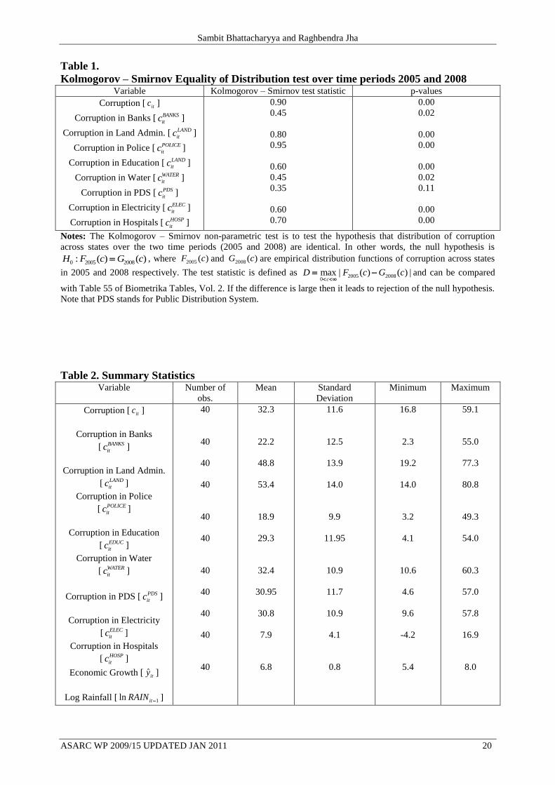
Detailed definitions and sources of all variables are available in Appendix A.1. Table 2
reports descriptive statistics of the major variables used in the study.
3. Empirical Evidence
Table 1 reports Kolmogorov-Smirnov test results for the equality of distributions of corruption
over the time periods 2005 and 2008. The test shows that the distribution of corruption across
states have changed over the two time periods. This may be driven by the variation in economic
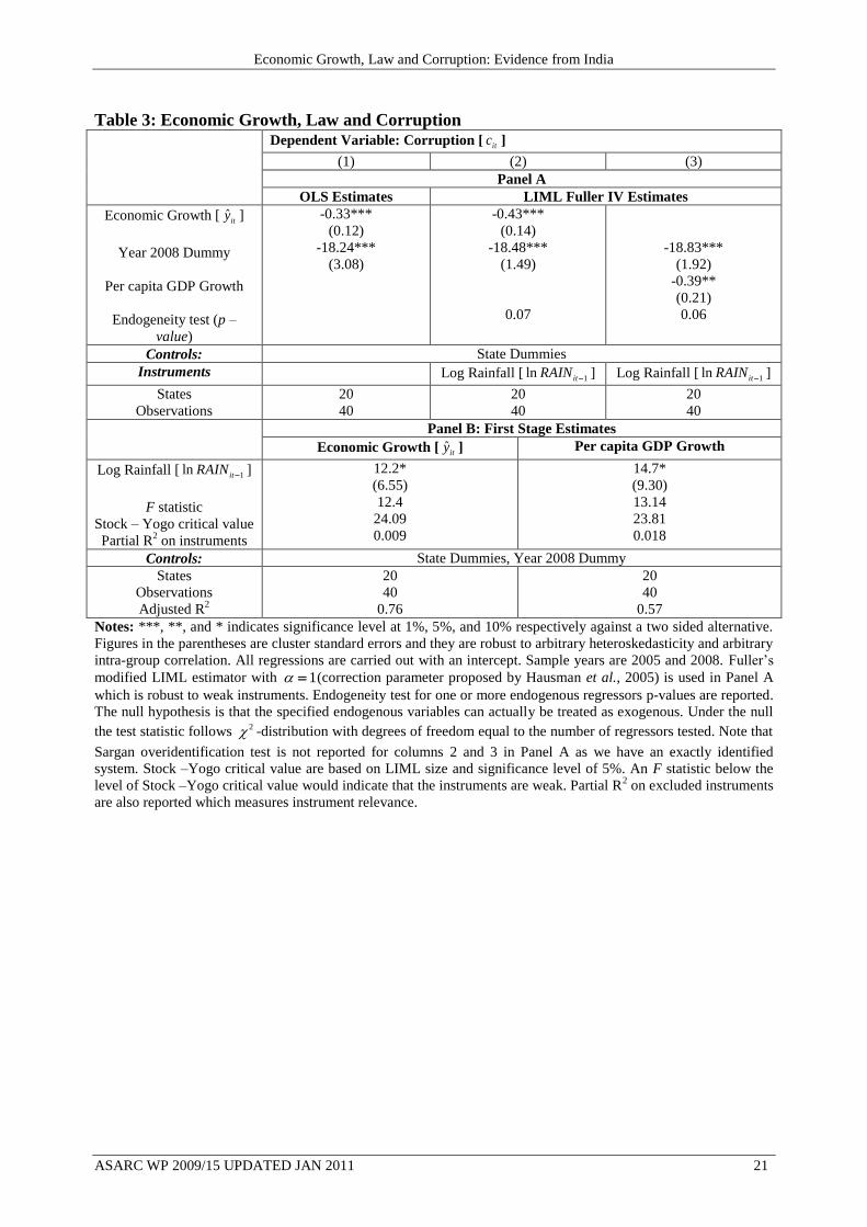
growth across states. In table 3 we try to find out by estimating equation (1) using OLS and
LIML Fuller instrumental variable method. Column 1 reports the OLS estimates and column 2
Sambit Bhattacharyya and Raghbendra Jha
ASARC WP 2009/15 UPDATED JAN 2011 10
presents estimates of the model using 1ln itRAIN as an instrument for economic growth. Our
suspicion that economic growth can be endogenous is supported by the endogeneity test reported
at the bottom of column 2. We notice that economic growth has a negative impact on corruption.
Ceteris paribus, one sample standard deviation (4.1 percentage points) increase in economic
growth in an average state would reduce corruption by 1.8 percentage points. In other words, our
model predicts that an increase in the growth rate of Bihar from -4.2 percent in 2005 to 16
percent in 2008 would reduce corruption from 59 percent in 2005 to 50.3 percent in 2008.
According to our dataset, Bihar‟s actual corruption in 2008 is 29 percent. Therefore, the
estimated coefficient on economic growth explains 29 percent of the actual decline in corruption
in Bihar over the period 2005 to 2008.
The coefficient on the year 2008 dummy captures the effect of RTI. Our estimates
suggest that RTI has a negative impact on corruption and the effect is statistically significant. In
particular, ceteris paribus the RTI Act reduces corruption in an average state by 18.5 percentage
points. To put this into perspective, the RTI Act explains approximately 62 percent of the actual
decline in corruption in Bihar over the period 2005 to 2008.8 This is indeed a large effect.
Note that IV coefficient estimates are typically larger than the OLS estimates. This is not
surprising given that IV estimates are correcting for the measurement error induced attenuation
bias in OLS.
In column 3 we use per capita GDP growth instead of aggregate GDP growth and our
result remains unaffected. Note that we also estimate the model using five year average growth
rates instead of economic growth over the periods 2004-2005 and 2007-2008. Our results are
robust to this test. Results are not reported here but are available upon request.
How good is our 1ln itRAIN instrument? Panel B in table 3 show that it is positively
correlated with economic growth. Therefore it can serve as an instrument provided it satisfies
the exclusion restriction. In other words, rainfall affects corruption exclusively through the
economic growth channel. However, rainfall may affect corruption through channels other than
economic growth. Poverty and inequality are such candidates. Rainfall may lead to reduction in
poverty, which may in turn lead to a reduction in corruption. Better rainfall and better
agriculture growth may also increase inequality leading to an increase in corruption. In such
situation, the exclusion restriction would be violated.
8 Model predicts that corruption in Bihar should have reduced by 18.5 percentage points due to the RTI Act. The
actual decline however is 30 percentage points. Therefore, the predicted decline is 62 percent of the actual.
Economic Growth, Law and Corruption: Evidence from India
ASARC WP 2009/15 UPDATED JAN 2011 11
Unfortunately there are no direct statistical tests for the exclusion restriction. However,
to eliminate the possibility of exclusion restriction violation we check the correlation between
the rainfall instrument and poverty and inequality. It turns out to be 0.17 and 0.38 respectively
which suggests it is unlikely that rainfall would affect corruption through poverty and inequality
channel. Therefore, we conclude that 1ln itRAIN can serve as a valid instrument.
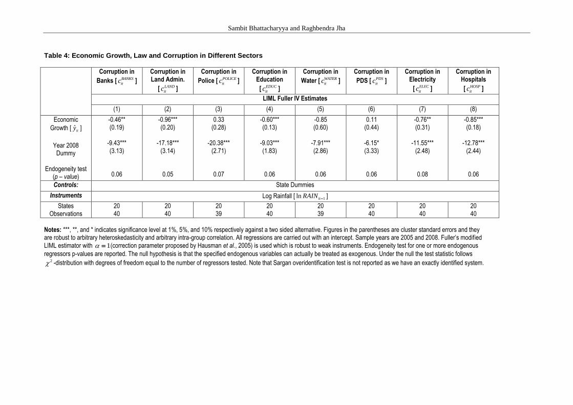
In table 4 we ask the question whether the effect of economic growth and law on
corruption is uniform across all sectors of the economy. In particular we look at corruption in
banking, land administration, police, education, water supply, public distribution system,
electricity, and hospitals. Indeed there are more sectors in an economy which may have chronic
corruption problem and we do admit that our list is far from being comprehensive. However it
should be noted that our study is the first attempt to look at corruption at a disaggregated level in
India using panel data and we are constrained by data availability. The results indicate that the
RTI Act had an impact on all sectors examined in this study. The magnitude of the predicted
decline however varies from a 20.4 percentage points in policing to 6.2 percentage points in the
public distribution system. In contrast the effect of economic growth is far from being uniform.
Banking, land administration, education, electricity, and hospitals register a statistically
significant negative effect of economic growth on corruption. The effect however is insignificant
in case of policing, water supply, and public distribution system.
In table 5 we check whether there is a difference between actual corruption experience
and corruption perception. Indeed we find that the effect of economic growth on corruption is
not uniform across actual experience and perception. Panel A reports estimates with actual
corruption experience. Note that corruption experience here is the average of answers to the
questions on „direct experience of bribing‟ and „using influence of a middleman‟. In addition to
affecting overall corruption experience, economic growth appears to reduce corruption
experiences in banking, land administration, education, electricity, and hospitals. The effects on
police, water supply, and public distribution system however is statistically insignificant. The
observed pattern is very similar to table 4. This suggests that our corruption results reported in
tables 3 and 4 are driven by actual corruption experiences. Panel B reports estimates with
corruption perception. Note that corruption perception here is the average of answers to the
questions on „perception that a department is corrupt‟ and „perception that corruption has
increased‟. We notice that economic growth has little effect on corruption perception9 and in
case of policing it appears to have increased corruption perception. This is in line with the view
9According to our estimates, economic growth reduced corruption perception only in education.
Sambit Bhattacharyya and Raghbendra Jha
ASARC WP 2009/15 UPDATED JAN 2011 12
that perpetual pessimism with regards to government services tends to shape corruption
perception in developing economies and any impact that economic growth may have on actual
corruption is often overlooked. Our result is broadly in line with the findings of Olken (2009)
who also report differences in corruption perception and corruption experience in Indonesia,
another developing economy.
The effect of RTI on corruption experience and corruption perception is somewhat
uniform. The magnitude of the effect however varies across sectors. We notice that the effect of
RTI on corruption experience is greater than its effect on corruption perception in case of overall
corruption, land administration, and public distribution system. In contrast, the reverse is
observed in case of banking, police, education, water supply, electricity, and hospitals.
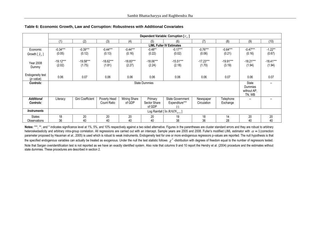
In table 6 we add additional covariates into our specification to address the issue of
omitted variables. In column 1 we add literacy as an additional control variable. The rationale is
that literate citizens are relatively more empowered to fight corruption. Our result survives.
Poverty and inequality may also increase corruption. To check whether this has any effect we
add Gini coefficient and poverty head count ratio as additional controls in columns 2 and 3. Our
result remains unaffected. Natural resources in general and resource rent in particular may also
increase corruption (see Ades and Di Tella, 1999; Treisman, 2000; Isham et al., 2005;
Bhattacharyya and Hodler, 2009). To check we add mining share of GDP and primary sector
share of GDP in columns 4 and 5 and our results are robust. High levels of government
expenditure may increase corruption as corrupt officials now have access to more resources to
usurp. It can also work in the opposite direction with the government now able to engage more
resources into auditing. Indeed we do notice evidence in support of the latter in column 6 with
state government expenditure having a significant negative impact on corruption. This is in line
with Olken (2007) who show that government audit reduces corruption in Indonesia.
Nevertheless, more importantly our economic growth and law results remain unaffected. In
column 7 we test whether controlling for the effect of media would alter our result. Media and
an active civil society may reduce corruption. We try to capture this effect using newspaper
circulation. Our main result survives. Column 8 tackles the view that telecommunication
revolution in India may have triggered this decline in corruption by eliminating the middleman
and reducing discretionary power of corrupt officials. To capture this effect we use number of
telephone exchanges as a control variable and our results survive.
In table 7 we put our results under further scrutiny. We test whether our results are
driven by influential observations. We identify influential observations using Cook‟s distance,

Economic Growth, Law and Corruption: Evidence from India
ASARC WP 2009/15 UPDATED JAN 2011 13
DFITS, and Welsch distance formula. The influential observations according to these formulas
are from Bihar, Kerala, and Madhya Pradesh. We estimate our model by omitting these
influential observations and our result remains unaffected.
Finally, in table 8 we test the robustness of our results with alternative instruments. Our
basic results survive when we use flood affected area, flood affected population, flood affected
crop area, and total number of flood affected households as alternative instruments. These
instruments are geography based and likely to be exogenous. They are also likely to satisfy the
exclusion restriction as it is hard to imagine them having an effect on corruption through any
channels other than economic growth.10
Nevertheless, they are not our preferred estimates as
they lead to a reduction in our sample size.
Overall these empirical findings support our prediction that both economic growth and
RTI have negative impacts on corruption. The effect of the RTI Act however is more uniform
than the effect of economic growth.
4. Concluding Remarks
We study the causal impact of economic growth and law on corruption. Using a novel panel
dataset covering 20 Indian states and the periods 2005 and 2008 we are able to estimate the
causal effects of economic growth and law on corruption. To tackle endogeneity concerns we
use rainfall as an instrument for economic growth. Rainfall is a positive predictor of growth
which is in line with the view that rainfall contributes positively to economic growth. It also
affects corruption through the economic growth channel reasonably exclusively. To capture the
effect of law on corruption we use a time dummy and control for other nationwide changes
which may be affecting corruption. Our results indicate that economic growth reduces overall
corruption as well as corruption in banking, land administration, education, electricity, and
hospitals. Growth however has little impact on corruption perception. In contrast the RTI
negatively impacts both corruption experience and corruption perception. Our basic result holds
after controlling for state fixed effects and various additional covariates (for example, literacy,
Gini coefficient, poverty head count ratio, mining share of state GDP, primary sector share of
state GDP, state government expenditure as a share of state GDP, newspaper circulation, and
number of telephone exchanges). It is also robust to the use of alternative instruments and outlier
sensitivity tests.
10
They can however affect corruption through poverty and inequality. We have checked the correlation between
these instruments and poverty and inequality and they are very low.
Sambit Bhattacharyya and Raghbendra Jha
ASARC WP 2009/15 UPDATED JAN 2011 14
The paper makes the following four original contributions. First, the paper presents the
first panel data study of economic growth and corruption covering Indian state. Second, using a
time dummy and exploiting the construction of the dataset the paper estimates the effect of the
RTI law on corruption in India. Third, using sector wise disaggregated data the paper estimates
the causal effect of economic growth and law on corruption in banking, land administration,
police, education, water supply, PDS, electricity, and hospitals. Fourth, the paper also separately
estimates the effects of growth and law on corruption experience and corruption perception and
finds that they are different.
Our results have important policy implications not just for India but also for other
comparable developing economies. Our findings imply that economic forces have an important
role in reducing corruption. Therefore macro policies to promote economic growth not only
improves overall living standard, it also enhances the quality of public goods by reducing
corruption. It perhaps works through the following channels. First, it provides the government
with additional resources to fight corruption. This is supported by the negative coefficient on the
state government expenditure variable reported in column 6, table 6.11
Second, it also reduces
the incentives for corruption at the micro level by raising the opportunity cost. More micro level
research is certainly called for to find out whether the data supports these conjectures.
Legislations such as the RTI Act in India are also important in curbing corruption. On
the one hand it empowers citizens‟ and breaks the information monopoly of the public officials.
Therefore, it prevents corrupt public officials from misusing this information to advance their
own interest. On the other hand it provides the government with more power and public support
for conducting top down audit of corrupt departments. There is evidence that the latter works
effectively in a developing economy environment (Olken, 2007).
Finally, more caution is required with the measurement of corruption. Our results
indicate that there is a fair bit of difference between actual corruption experience and corruption
perception in developing economies. Therefore over reliance on one or the other may be
counterproductive. We do not stand alone on this as other studies also indicate that perception
and actual corruption tends to vary significantly (Olken, 2009). Measuring corruption
appropriately in our view is crucial in furthering our understanding of corruption.
11
See Fisman and Gatti (2002) for an alternative view. They show that fiscal decentralization and larger
government revenue leads to higher corruption using international data.
Economic Growth, Law and Corruption: Evidence from India
ASARC WP 2009/15 UPDATED JAN 2011 15
Appendix A
A.1 Data description
Corruption [ itc ]: Corruption is computed using a two step procedure. First, an average is
computed of the percentage of respondents answering yes to the questions that they have direct
experience of bribing, using a middleman, perception that a department is corrupt, and
perception that corruption increased over time for 8 different sectors (banking, land
administration, police, education, water, Public Distribution System (PDS), electricity, and
hospitals). Second, these averages are also averaged over all the 8 sectors to generate one
observation per state and per time period. Higher value of the corruption measure implies higher
corruption. Source: India Corruption Study 2005 and 2008, Transparency International.
Corruption in Banks [BANKS
itc ]: Corruption computed in the same fashion as itc but only for the
banking sector. Source: India Corruption Study 2005 and 2008, Transparency International.
Corruption in Land Administration [LAND
itc ]: Corruption computed in the same fashion as itc but
only for the land administration sector. Source: India Corruption Study 2005 and 2008,
Transparency International.
Corruption in Police [POLICE
itc ]: Corruption computed in the same fashion as itc but only for
police. Source: India Corruption Study 2005 and 2008, Transparency International.
Corruption in Education [EDUC
itc ]: Corruption computed in the same fashion as itc but only for
education sector. Source: India Corruption Study 2005 and 2008, Transparency International.
Corruption in Water [WATER
itc ]: Corruption computed in the same fashion as itc but only for the
water supply sector. Source: India Corruption Study 2005 and 2008, Transparency International.
Corruption in PDS [PDS
itc ]: Corruption computed in the same fashion as itc but only for the public
distribution system. Source: India Corruption Study 2005 and 2008, Transparency International.
Corruption in Electricity [ELEC
itc ]: Corruption computed in the same fashion as itc but only for the
electricity sector. Source: India Corruption Study 2005 and 2008, Transparency International.
Corruption in Hospitals [HOSP
itc ]: Corruption computed in the same fashion as itc but only for
hospitals. Source: India Corruption Study 2005 and 2008, Transparency International.
Corruption Experience Measures: Corruption experience measures are the average of answers to
the questions on „direct experience of bribing‟ and „using influence of a middleman‟. Source:
India Corruption Study 2005 and 2008, Transparency International.
Sambit Bhattacharyya and Raghbendra Jha
ASARC WP 2009/15 UPDATED JAN 2011 16
Corruption Perception Measures: Corruption perception measures are the average of answers to
the questions on „perception that a department is corrupt‟ and „perception that corruption has
increased‟. Source: India Corruption Study 2005 and 2008, Transparency International.
Economic Growth [ ˆity ]: Real growth rate in state GDP measured in 2009 constant prices.
Source: Planning Commission, Government of India.
Log Rainfall [ 1ln itRAIN ]: Log of rainfall across states measured in millimeters. Source:
Compendium of Environmental Statistics, Central Statistical Organisation, Ministry of Statistics
and Programme Implementation.
Flood Area: Total area affected by flood in 1994 and 1996 measured in millions of hectares.
Source: Central Water Commission, Government of India.
Flood Population: Total population affected by flood in 1994 and 1996 measured in millions.
Source: Central Water Commission, Government of India.
Flood Crop Area: Total crop area affected by flood in 1994 and 1996 measured in millions of
hectares. Source: Central Water Commission, Government of India.
Flood Household: Total number of households affected by flood in 1994 and 1996 measured in
millions of hectares. Source: Central Water Commission, Government of India.
Literacy: Literacy rate for 2002 and 2005. Source: Selected Socioeconomic Statistics India
2006, Central Statistical Organization, Table 3.3.
Gini Coefficient: Gini coefficient urban for the periods 1999-2000 and 2004-05. Source:
Planning Commission.
Poverty Head Count Ratio: Percentage of population below poverty line (rural and urban
combined). Source: Planning Commission.
Mining Share of GDP: Mining sector share of state GDP. Source: Handbook of Statistics on the
Indian Economy, Reserve Bank of India.
Primary Sector Share of GDP: Primary sector share of state GDP. Source: Handbook of
Statistics on the Indian Economy, Reserve Bank of India.4
State Government Expenditure: State government expenditure as a proportion of state GDP.
Source: Indian Public Finance Statistics, Ministry of Finance.
Newspaper Circulation: Number of registered newspapers in circulation. Source: Registrar of
Newspapers, Government of India.
Telephone Exchange: Number of telephone exchanges. Source: Ministry of Information and
Broadcasting, Government of India.

Economic Growth, Law and Corruption: Evidence from India
ASARC WP 2009/15 UPDATED JAN 2011 17
A.2 Sample and State Codes
Andhra Pradesh (AP), Assam (AS), Bihar (BH), Chhattisgarh (CG), Delhi (DL), Gujarat (GJ),
Haryana (HR), Himachal Pradesh (HP), Jammu and Kashmir (JK), Jharkhand (JH), Karnataka
(KT), Kerala (KL), Madhya Pradesh (MP), Maharashtra (MH), Orissa (OS), Punjab (PJ),
Rajasthan (RJ), Tamil Nadu (TN), Uttar Pradesh (UP), West Bengal (WB).

Sambit Bhattacharyya and Raghbendra Jha
ASARC WP 2009/15 UPDATED JAN 2011 18
References
Acemoglu, D., S. Johnson, and J. Robinson. (2001). “The colonial origins of comparative development: an
empirical investigation,” American Economic Review, 91(5), 1369-1401.
Ades, A., and R. Di Tella. (1999). “Rents, Competition, and Corruption,” American Economic Review, 89(4), 982-
993.
Bardhan, P. (1997). “Corruption and Development: A Review of Issues,” Journal of Economic Literature, 35(3),
1320 – 1346.
Belsley, D., E. Kuh, and R. Welsch. (1980). “Regressions Diagnostics: Identifying Influential Data and Sources of
Collinearity,” New York: John Wiley & Sons.
Besley, T., and R. Burgess. (2000). “Land Reform, Poverty Reduction and Growth: Evidence From India,”
Quarterly Journal of Economics, 115(2), 389-430.
Besley, T., and R. Burgess. (2004). “Can Labor Regulation Hinder Economic Performance? Evidence From India,”
Quarterly Journal of Economics, 119(1), 91-134.
Bhattacharyya, S. (2009). “Unbundled Institutions, Human Capital and Growth,” Journal of Comparative
Economics, 37, 106 – 120.
Bhattacharyya, S., and R. Hodler (2010). “Natural Resources, Democracy and Corruption,” European Economic
Review, 54, 608 – 621.
Dabla-Norris, E. (2000). “A Game – Theoretic Analysis of Corruption in Bureaucracies,” IMF Working Paper No.
WP/00/106.
Fan, S., C. Lin, and D. Treisman. (2009). “Political Decentralization and Corruption: Evidence from Around the
World,” Journal of Public Economics, 93, 14-34.
Fisman, R., and R. Gatti. (2002). “Decentralization and Corruption: Evidence Across Countries,” Journal of Public
Economics, 83(3), 325-345.
Hall, R., and C. Jones. (1999). “Why do some countries produce so much more output per worker than others?”
Quarterly Journal of Economics, 114(1), pp. 83-116.
Hausman, J., J. Stock, and M. Yogo. (2005). “Asymptotic Properties of the Hahn-Hausman Test for Weak
Instruments,” Economics Letters, 89(3), 333-342.
Hendry, D., S. Johansen, and C. Santos. (2004). “Selecting a Regression Saturated by Indicators,” University of
Oxford, Unpublished Manuscript.
Isham, J., L. Pritchett, M. Woolcock, and G. Busby. (2005). “The Varieties of Resource Experience: Natural
Resource Export Structures and the Political Economy of Economic Growth,” World Bank Economic
Review, 19, 141-174.
Knack, S., and P. Keefer. (1995). “Institutions and Economic Performance: Cross-Country Tests using Alternative
Institutional Measures,” Economics and Politics, 7, 207-227.
Leite, C., and J. Weidmann. (1999). “Does Mother Nature Corrupt? Natural Resources, Corruption and Economic
Growth,” IMF Working Paper No. WP/99/85.
Mauro, P. (1995). “Corruption and Growth,” Quarterly Journal of Economics, 110, 681-712.
Olken, B. (2007). “Monitoring Corruption: Evidence from a Field Experiment in Indonesia,” Journal of Political
Economy, 115(2), 200-249.
Olken, B. (2009). “Corruption Perceptions vs. Corruption Reality,” Journal of Public Economics, 93, 950-964.
Rodrik, D., A. Subramanian, and F. Trebbi. (2004). “Institutions Rule: the Primacy of Institutions over Geography
and Integration in Economic Development,” Journal of Economic Growth, 9, 131-165.
Rose-Ackerman, S. (1999). “Corruption and Government: Causes, Consequences and Reform,” Cambridge
University Press: Cambridge.
Staiger, D. and J. Stock. (1997). “Instrumental Variables Regression with Weak Instruments,” Econometrica, 65,
557-586.
Stock, J. and M. Yogo. (2005). “Testing for Weak Instruments in Linear IV Regression,” in D. Andrews and J.
Stock, eds., Identification and Inference for Econometric Models: Essays in Honor of Thomas Rothenberg,
Cambridge: Cambridge University Press, 2005, pp. 80–108.
Treisman, D. (2000). “The Causes of Corruption: A Cross-National Study,” Journal of Public Economics, 76, 399 –
457.
Economic Growth, Law and Corruption: Evidence from India
ASARC WP 2009/15 UPDATED JAN 2011 19
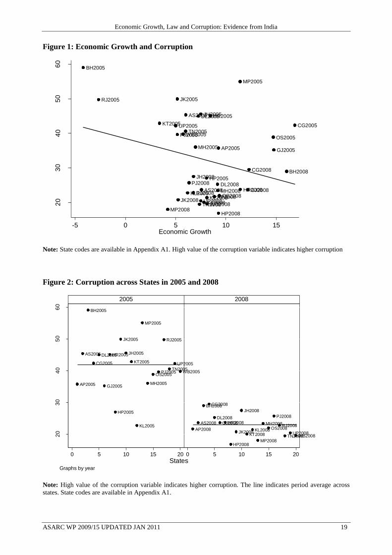
Figure 1: Economic Growth and Corruption
AP2005
AP2008
AS2005
AS2008
BH2005
BH2008
CG2005
CG2008
DL2005
DL2008
GJ2005
GJ2008
HR2005
HR2008
HP2005
HP2008
JK2005
JK2008
JH2005
JH2008
KT2005
KT2008
KL2005KL2008
MP2005
MP2008
MH2005
MH2008
OS2005
OS2008
PJ2005
PJ2008
RJ2005
RJ2008
TN2005
TN2008
UP2005
UP2008
WB2005
WB200820
30
40
50
60
Corr
uptio
n
-5 0 5 10 15Economic Growth
Note: State codes are available in Appendix A1. High value of the corruption variable indicates higher corruption
Figure 2: Corruption across States in 2005 and 2008
AP2005
AS2005
BH2005
CG2005
DL2005
GJ2005
HR2005
HP2005
JK2005
JH2005
KT2005
KL2005
MP2005
MH2005
OS2005PJ2005
RJ2005
TN2005
UP2005
WB2005
AP2008
AS2008
BH2008CG2008
DL2008
GJ2008HR2008
HP2008
JK2008
JH2008
KT2008KL2008
MP2008
MH2008OS2008
PJ2008
RJ2008
TN2008UP2008
WB200820
30
40
50
60
0 5 10 15 20 0 5 10 15 20
2005 2008
Corr
uptio
n
StatesGraphs by year
Note: High value of the corruption variable indicates higher corruption. The line indicates period average across
states. State codes are available in Appendix A1.
Sambit Bhattacharyya and Raghbendra Jha
ASARC WP 2009/15 UPDATED JAN 2011 20
Table 1.
Kolmogorov – Smirnov Equality of Distribution test over time periods 2005 and 2008 Variable Kolmogorov – Smirnov test statistic p-values
Corruption [ itc ]
Corruption in Banks [ BANKS
itc ]
Corruption in Land Admin. [ LAND
itc ]
Corruption in Police [ POLICE
itc ]
Corruption in Education [ LAND
itc ]
Corruption in Water [ WATER
itc ]
Corruption in PDS [ PDS
itc ]
Corruption in Electricity [ ELEC
itc ]
Corruption in Hospitals [ HOSP
itc ]
0.90
0.45
0.80
0.95
0.60
0.45
0.35
0.60
0.70
0.00
0.02
0.00
0.00
0.00
0.02
0.11
0.00
0.00
Notes: The Kolmogorov – Smirnov non-parametric test is to test the hypothesis that distribution of corruption
across states over the two time periods (2005 and 2008) are identical. In other words, the null hypothesis is
0 2005 2008: ( ) ( )H F c G c , where 2005 ( )F c and 2008 ( )G c are empirical distribution functions of corruption across states
in 2005 and 2008 respectively. The test statistic is defined as 2005 20080max | ( ) ( ) |
cD F c G c
and can be compared
with Table 55 of Biometrika Tables, Vol. 2. If the difference is large then it leads to rejection of the null hypothesis.
Note that PDS stands for Public Distribution System.
Table 2. Summary Statistics
Variable Number of
obs.
Mean Standard
Deviation
Minimum Maximum
Corruption [ itc ]
Corruption in Banks
[ BANKS
itc ]
Corruption in Land Admin.
[ LAND
itc ]
Corruption in Police
[ POLICE
itc ]
Corruption in Education
[ EDUC
itc ]
Corruption in Water
[ WATER
itc ]
Corruption in PDS [ PDS
itc ]
Corruption in Electricity
[ ELEC
itc ]
Corruption in Hospitals
[ HOSP
itc ]
Economic Growth [ ˆity ]
Log Rainfall [ 1ln itRAIN ]
40
40
40
40
40
40
40
40
40
40
40
32.3
22.2
48.8
53.4
18.9
29.3
32.4
30.95
30.8
7.9
6.8
11.6
12.5
13.9
14.0
9.9
11.95
10.9
11.7
10.9
4.1
0.8
16.8
2.3
19.2
14.0
3.2
4.1
10.6
4.6
9.6
-4.2
5.4
59.1
55.0
77.3
80.8
49.3
54.0
60.3
57.0
57.8
16.9
8.0
Economic Growth, Law and Corruption: Evidence from India
ASARC WP 2009/15 UPDATED JAN 2011 21
Table 3: Economic Growth, Law and Corruption
Dependent Variable: Corruption [ itc ]
(1) (2) (3)
Panel A
OLS Estimates LIML Fuller IV Estimates
Economic Growth [ ˆity ]
Year 2008 Dummy
Per capita GDP Growth
Endogeneity test (p –
value)
-0.33***
(0.12)
-18.24***
(3.08)
-0.43***
(0.14)
-18.48***
(1.49)
0.07
-18.83***
(1.92)
-0.39**
(0.21)
0.06
Controls: State Dummies
Instruments Log Rainfall [ 1ln itRAIN ] Log Rainfall [ 1ln itRAIN ]
States
Observations
20
40
20
40
20
40
Panel B: First Stage Estimates
Economic Growth [ ˆity ] Per capita GDP Growth
Log Rainfall [ 1ln itRAIN ]
F statistic
Stock – Yogo critical value
Partial R2 on instruments
12.2*
(6.55)
12.4
24.09
0.009
14.7*
(9.30)
13.14
23.81
0.018
Controls: State Dummies, Year 2008 Dummy
States
Observations
Adjusted R2
20
40
0.76
20
40
0.57
Notes: ***, **, and * indicates significance level at 1%, 5%, and 10% respectively against a two sided alternative.
Figures in the parentheses are cluster standard errors and they are robust to arbitrary heteroskedasticity and arbitrary
intra-group correlation. All regressions are carried out with an intercept. Sample years are 2005 and 2008. Fuller‟s
modified LIML estimator with 1 (correction parameter proposed by Hausman et al., 2005) is used in Panel A
which is robust to weak instruments. Endogeneity test for one or more endogenous regressors p-values are reported.
The null hypothesis is that the specified endogenous variables can actually be treated as exogenous. Under the null
the test statistic follows 2 -distribution with degrees of freedom equal to the number of regressors tested. Note that
Sargan overidentification test is not reported for columns 2 and 3 in Panel A as we have an exactly identified
system. Stock –Yogo critical value are based on LIML size and significance level of 5%. An F statistic below the
level of Stock –Yogo critical value would indicate that the instruments are weak. Partial R2 on excluded instruments
are also reported which measures instrument relevance.
Sambit Bhattacharyya and Raghbendra Jha
Table 4: Economic Growth, Law and Corruption in Different Sectors
Corruption in
Banks [ BANKS
itc ]
Corruption in Land Admin.
[ LAND
itc ]
Corruption in
Police [ POLICE
itc ]
Corruption in Education
[ EDUC
itc ]
Corruption in
Water [ WATER
itc ]
Corruption in
PDS [ PDS
itc ]
Corruption in Electricity
[ ELEC
itc ]
Corruption in Hospitals
[ HOSP
itc ]
LIML Fuller IV Estimates
(1) (2) (3) (4) (5) (6) (7) (8)
Economic
Growth [ ˆity ]
Year 2008
Dummy
Endogeneity test (p – value)
-0.46** (0.19)
-9.43*** (3.13)
0.06
-0.96*** (0.20)
-17.18***
(3.14)
0.05
0.33 (0.28)
-20.38***
(2.71)
0.07
-0.60*** (0.13)
-9.03*** (1.83)
0.06
-0.85 (0.60)
-7.91*** (2.86)
0.06
0.11 (0.44)
-6.15* (3.33)
0.06
-0.76** (0.31)
-11.55***
(2.48)
0.08
-0.85*** (0.18)
-12.78***
(2.44)
0.06
Controls: State Dummies
Instruments Log Rainfall [ 1ln itRAIN ]
States Observations
20 40
20 40
20 39
20 40
20 39
20 40
20 40
20 40
Notes: ***, **, and * indicates significance level at 1%, 5%, and 10% respectively against a two sided alternative. Figures in the parentheses are cluster standard errors and they are robust to arbitrary heteroskedasticity and arbitrary intra-group correlation. All regressions are carried out with an intercept. Sample years are 2005 and 2008. Fuller’s modified
LIML estimator with 1 (correction parameter proposed by Hausman et al., 2005) is used which is robust to weak instruments. Endogeneity test for one or more endogenous
regressors p-values are reported. The null hypothesis is that the specified endogenous variables can actually be treated as exogenous. Under the null the test statistic follows 2 -distribution with degrees of freedom equal to the number of regressors tested. Note that Sargan overidentification test is not reported as we have an exactly identified system.

Table 5: Effect of Economic Growth and Law on Corruption Experience and Corruption Perception
Corruption Experience
overall
Corruption Experience in
Banks
Corruption Experience in Land Admin.
Corruption Experience in
Police
Corruption Experience in
Education
Corruption Experience in
Water
Corruption Experience in
PDS
Corruption Experience in
Electricity
Corruption Experience in
Hospitals
Panel A: LIML Fuller IV Estimates with Corruption Experience
(1) (2) (3) (4) (5) (6) (7) (8) (9)
Economic Growth
[ ˆity ]
Year 2008
Dummy
Endogeneity test (p–value)
-0.92*** (0.21)
-17.09***
(2.05)
0.06
-0.77*** (0.25)
-11.55***
(2.19)
0.06
-1.66*** (0.59)
-29.25***
(4.99)
0.08
-0.19 (0.58)
-12.09***
(4.49)
0.05
-0.87*** (0.09)
-7.55*** (1.47)
0.04
-0.80 (0.87)
-7.65** (3.81)
0.05
-0.13 (0.37)
-10.39***
(3.31)
0.06
-0.97*** (0.29)
-11.04***
(1.93)
0.06
-1.79*** (0.34)
-7.22*** (2.74)
0.06
Controls: State Dummies
Instruments Log Rainfall [ 1ln itRAIN ]
States Observations
20 40
20 40
20 40
20 39
20 40
20 39
20 40
20 40
20 40
Corruption Perception
overall
Corruption Perception in
Banks
Corruption Perception in Land Admin.
Corruption Perception in
Police
Corruption Perception in
Education
Corruption Perception in
Water
Corruption Perception in
PDS
Corruption Perception in
Electricity
Corruption Perception in
Hospitals
Panel B: LIML Fuller IV Estimates with Corruption Perception
Economic Growth
[ ˆity ]
Year 2008
Dummy
Endogeneity test (p–value)
-0.21 (0.36)
-15.35***
(2.86)
0.06
-0.11 (0.45)
-14.42** (5.95)
0.06
-0.83 (0.62)
-12.17***
(4.11)
0.07
0.72* (0.37)
-14.27***
(3.69)
0.05
-0.64* (0.34)
-14.54***
(2.77)
0.03
-0.84 (0.96)
-12.47***
(4.73)
0.06
0.05 (0.65)
-6.67 (4.44)
0.05
-0.62 (0.54)
-19.14***
(3.83)
0.06
0.22 (0.41)
-18.12***
(2.59)
0.06
Controls: State Dummies
Instruments Log Rainfall [ 1ln itRAIN ]
States Observations
20 40
20 40
20 40
20 39
20 40
20 39
20 40
20 40
20 40
Notes: ***, **, and * indicates significance level at 1%, 5%, and 10% respectively against a two sided alternative. Figures in the parentheses are cluster standard errors and they are robust to arbitrary heteroskedasticity and arbitrary intra-group correlation. All regressions are carried out with an intercept. Sample years are 2005 and 2008. Fuller’s modified LIML estimator with
1 (correction parameter proposed by Hausman et al., 2005) is used which is robust to weak instruments. Endogeneity test for one or more endogenous regressors p-values are reported. The
null hypothesis is that the specified endogenous variables can actually be treated as exogenous. Under the null the test statistic follows 2 -distribution with degrees of freedom equal to the number
of regressors tested. Note that Sargan overidentification test is not reported as we have an exactly identified system.
Sambit Bhattacharyya and Raghbendra Jha
Table 6: Economic Growth, Law and Corruption: Robustness with Additional Covariates
Dependent Variable: Corruption [ itc ]
(1) (2) (3) (4) (5) (6) (7) (8) (9) (10)
LIML Fuller IV Estimates
Economic
Growth [ ˆity ]
Year 2008
Dummy
Endogeneity test (p–value)
-0.34*** (0.05)
-19.12***
(2.02)
0.06
-0.39*** (0.12)
-19.58***
(1.75)
0.07
-0.44*** (0.13)
-18.62***
(1.81)
0.06
-0.44*** (0.16)
-18.83***
(2.27)
0.06
-0.48** (0.22)
-18.06***
(2.24)
0.06
-0.17*** (0.02)
-15.51***
(2.18)
0.06
-0.76*** (0.06)
-17.23***
(1.70)
0.06
-0.64*** (0.21)
-19.91***
(3.19)
0.07
-0.47*** (0.16)
-18.21***
(1.94)
0.06
-1.22** (0.67)
-18.41***
(1.94)
0.07
Controls: State Dummies State Dummies
without AP, TN, WB
--
Additional Controls:
Literacy Gini Coefficient Poverty Head Count Ratio
Mining Share of GDP
Primary Sector Share
of GDP
State Government Expenditure***
(-)
Newspaper Circulation
Telephone Exchange
-- --
Instruments Log Rainfall [ 1ln itRAIN ]
States Observations
18 36
20 40
20 40
20 40
20 40
19 38
18 36
14 28
20 40
20 40
Notes: ***, **, and * indicates significance level at 1%, 5%, and 10% respectively against a two sided alternative. Figures in the parentheses are cluster standard errors and they are robust to arbitrary
heteroskedasticity and arbitrary intra-group correlation. All regressions are carried out with an intercept. Sample years are 2005 and 2008. Fuller’s modified LIML estimator with 1 (correction
parameter proposed by Hausman et al., 2005) is used which is robust to weak instruments. Endogeneity test for one or more endogenous regressors p-values are reported. The null hypothesis is that
the specified endogenous variables can actually be treated as exogenous. Under the null the test statistic follows 2 -distribution with degrees of freedom equal to the number of regressors tested.
Note that Sargan overidentification test is not reported as we have an exactly identified system. Also note that columns 9 and 10 report the Hendry et al. (2004) procedure and the estimates without state dummies. These procedures are described in section 2.

Table 7: Economic Growth, Law and Corruption: Robustness with Alternative Samples
Dependent Variable: Corruption [ itc ]
(1) (2) (3)
LIML Fuller IV Estimates
Economic Growth [ ˆity ]
Year 2008 Dummy
Endogeneity test (p–value)
-1.37*** (0.50)
-17.13*** (1.61) 0.06
-1.37*** (0.50)
-17.13*** (1.61) 0.06
-1.37*** (0.50)
-17.13*** (1.61) 0.06
Controls: State Dummies
Instruments Log Rainfall [ 1ln itRAIN ]
Omitted Observations Obs. Omitted using Cook’s Distance
Obs. Omitted using DFITS Obs. Omitted using Welsch Distance
States Observations
17 34
17 34
17 34
Notes: ***, **, and * indicates significance level at 1%, 5%, and 10% respectively against a two sided alternative. Figures in the parentheses are cluster standard errors and they are robust to arbitrary heteroskedasticity and arbitrary intra-group correlation. All regressions are carried
out with an intercept. Sample years are 2005 and 2008. Fuller’s modified LIML estimator with 1 (correction parameter proposed by
Hausman et al., 2005) is used which is robust to weak instruments. Endogeneity test for one or more endogenous regressors p-values are reported. The null hypothesis is that the specified endogenous variables can actually be treated as exogenous. Under the null the test statistic
follows 2 -distribution with degrees of freedom equal to the number of regressors tested. Note that Sargan overidentification test is not
reported as we have an exactly identified system. In column 1, omit if 4 /iCooksd n ; in column 2, omit if 2 /iDFITS k n ; and in
column 3, omit if 3iWelschd k formulas are used (see Belsley et al., 1980). Here n is the number of observation and k is the number
of independent variables including the intercept. Note that the Cook’s Distance, DFITS, and Welch Distance are calculated using the OLS version of the model (ie., table2, column 3). The influential observations according to the Cook’s Distance, DFITS, and Welsch Distance formula are BH2005, BH2008, KL2005, KL2008, MP2005, MP2008.
Table 8: Economic Growth, Law and Corruption: Robustness with Alternative Instruments
Dependent Variable: Corruption [ itc ]
(1) (2) (3) (4)
LIML Fuller IV Estimates
Economic Growth [ ˆity ]
Year 2008 Dummy
Endogeneity test (p–
value)
-0.94** (0.46)
-18.14***
(2.55)
0.04
-0.87* (0.44)
-18.29***
(2.29)
0.06
-0.56* (0.34)
-18.73***
(1.84)
0.06
-0.76*** (0.27)
-18.16***
(1.69)
0.07
Controls: State Dummies
Instruments Flood Area Flood Population Flood Crop Area Flood Households
States Observations
16 32
16 32
16 32
16 32
Notes: ***, **, and * indicates significance level at 1%, 5%, and 10% respectively against a two sided alternative. Figures in the parentheses are cluster standard errors and they are robust to arbitrary heteroskedasticity and arbitrary intra-group correlation. All regressions are carried
out with an intercept. Sample years are 2005 and 2008. Fuller’s modified LIML estimator with 1 (correction parameter proposed by
Hausman et al., 2005) is used which is robust to weak instruments. Endogeneity test for one or more endogenous regressors p-values are reported. The null hypothesis is that the specified endogenous variables can actually be treated as exogenous. Under the null the test statistic
follows 2 -distribution with degrees of freedom equal to the number of regressors tested. Note that Sargan overidentification test is not
reported as we have an exactly identified system.