Economic Feasibility of a Woody Biomass- Based Ethanol ... · Economic Feasibility of a Woody...

Journal of Agricultural and Resource Economics 35(3):522–544 Copyright 2010 Western Agricultural Economics Association

Economic Feasibility of a Woody Biomass- Based Ethanol Plant in Central Appalachia

Jinzhuo Wu, Mark Sperow, and Jingxin Wang

A mixed-integer programming model is developed to assess the economic feasibility of siting a woody biomass-based ethanol facility in the central Appalachian hardwood region. The model maximizes the net present value (NPV) of a facility over its economic life. Model inputs include biomass availability, biomass handling system type, plant investment and capacity, transportation logistics, feedstock and product pricing, project financing, and taxes. Four alternative woody biomass handling systems, which include all processes from stand to plant, are considered. Eleven possible plant locations were identified based on site selection requirements. Results showed that the optimal plant location was in Buckhannon, West Virginia. The NPV of the plant with a demand of 2,000 dry tons of woody biomass per day varied from $68.11 million to $84.51 million among the systems over a 20-year plant life. Internal rate of return (IRR) of the facility averaged 18.67% for the base case scenario. Average ethanol production costs were approximately $2.02 to $2.08 per gallon. Production costs were most impacted by biomass availability, mill residue purchase price, plant investment and capacity, ethanol yield, and financing. Findings suggest that a woody biomass-based ethanol facility in central Appalachia could be economically feasible under certain operational scenarios. Key Words: biofuels, economic analysis, ethanol, optimization, woody biomass

Introduction Interest in using biomass as feedstock for biofuel production in the United States has been increasing recently due to concerns about volatile oil prices, climate change, and the impact of diverting crops from food to fuel. Wood-based biomass—including residues produced during timber harvesting, fuelwood extracted from forestlands, and residues generated at primary and secondary wood processing facilities (Wang, Grushecky, and McNeel, 2006)—is a potentially important feedstock for biofuels (Perlack et al., 2005). A variety of liquid fuels can be produced from woody biomass, and ethanol is one of the most promising (Tyner and Taheripour, 2007). Most ethanol currently produced in the United States derives from corn fermentation; diverting corn from food to fuel has been linked to increased food prices (Taheripour and Tyner, 2008). Cellulose ethanol, a type of biofuel produced from lignocellulose, has many of the advan-tages of corn-based ethanol, including sustainability and cleanliness, but can be made from a variety of nonfood raw materials such as corn stover, switchgrass, and woody biomass. Laboratory testing has demonstrated that converting woody biomass into ethanol is techni-cally feasible (Zerbe, 1991). However, the economic viability of a commercial-scale woody

Jinzhuo Wu is graduate research assistant, Division of Forestry and Natural Resources; Mark Sperow is associate professor, Division of Resource Management; and Jingxin Wang (the paper’s corresponding author) is associate professor, Division of Forestry and Natural Resources, all at West Virginia University. This research was conducted under West Virginia EPSCOR Agreement No. EPS2006-35, and is published with the approval of the Director of the West Virginia Agricultural and Forestry Experiment Station as Scientific Article No. 3071. The authors are grateful to the anonymous Journal reviewers and the editor for providing helpful comments. Review coordinated by Myles J. Watts.

Wu, Sperow, and Wang Feasibility of a Woody Biomass-Based Ethanol Plant 523

biomass-based ethanol plant has not been fully addressed. Our economic feasibility study of biomass-based facilities considers investment, operating costs, time value of money, and quality of available data. We also include a sensitivity analysis to assess the robustness of the results. Several studies estimating the economic feasibility of cellulosic biomass utilization for bio-energy or biofuels have been conducted in the United States. Nienow et al. (1999) and Nienow, McNamara, and Gillespie (2000) estimated the cost of woody biomass (Salix tree) co-firing with coal for electricity production. They used a linear programming model to optimize the co-firing blend of coal and biomass while minimizing material procurement and ash disposal costs. Kaylen et al. (2000) constructed a mathematical model to analyze the economic feasibility of producing ethanol from lignocellulosic feedstocks (crop residues and woody biomass) by considering four cost modules, including capital cost, operating cost, feedstock cost, and transportation cost. Optimal ethanol plant size was determined by the tradeoff between increasing transportation costs for feedstock versus decreasing average plant costs as plant size increases. Kaylen et al. found that the optimally sized plant used 4,360 dry tons of feedstock, primarily crop residues with some woody biomass, per day. However, none of these studies considered the timing issues of feedstock handling activities. Tembo, Epplin, and Huhnke (2003) developed a multi-region, multi-period, mixed-integer mathematical programming model encompassing alternative feedstocks, feedstock production, delivery, and processing methods. Their model determined the most economically efficient source of lignocellulosic biomass (LCB), timing of harvest and storage, inventory manage-ment, and biorefinery size and location for a gasification-fermentation process. Five large (100 million gallons per year) and one medium (50 million gallons per year) biorefineries were optimally located with an expected net present value (NPV) of $1,143 million over a 15-year plant life. Mapemba et al. (2007, 2008) made some modifications to Tembo, Epplin, and Huhnke’s model. Incorporating harvesting systems and suitable monthly harvest days into the model, Mapemba et al. (2007) applied them to biomass harvested on Conservation Reserve Program land. They examined the cost to produce, harvest, store, and transport a flow of LCB, and how policies that restrict harvest frequency and the number of harvest days influence cost. In a related study, Mapemba et al. (2008) evaluated how the method of modeling harvest cost affects the number of harvest machines and the estimated cost to deliver LCB to a biorefinery. These studies did not consider typical activities involved in handling woody bio-mass. Other studies have performed economic analyses of an LCB-to-ethanol plant using Geographic Information System (GIS) data. Graham, English, and Noon (2000) used GIS to estimate the cost and environmental implications of supplying specific amounts of energy crop feedstock to a biorefinery. Noon, Zhan, and Graham (2002) identified candidate switchgrass-to-ethanol conversion plant locations using GIS-based analysis of marginal price (delivered cost) variation in Alabama. Although the GIS models can provide a visual repre-sentation, the results tend to be static, and other site selection criteria, such as availability of utilities and access to preexisting infrastructure, have not been considered. A 2006 study performed by Wang, Grushecky, and McNeel through West Virginia University’s Biomaterials Center provides an overview of West Virginia’s biomass resources, uses, and opportunities. They note that West Virginia ranks third nationally in percentage of forested land. The harvesting process yields approximately 2.41 million dry tons of wood residues annually. A small portion of logging residue is used for firewood or other purposes, but there are no statistical data to indicate the current total amount of logging residue used

524 December 2010 Journal of Agricultural and Resource Economics annually in West Virginia. Current practice leaves most of the residues scattered on the harvest sites. The authors report that the demand/supply ratio of mill residue in West Virginia averaged 68% in 2005, and there is a growing interest in more efficient wood residue utiliza-tion and conversion to biofuels. No commercial-scale woody biomass-based biofuel facility currently operates in the state. Wang, Grushecky, and McNeel conclude that industries with the likelihood of using woody biomass as a feedstock—such as biorefining, biochemicals, and biopolymers—have limited start-up potential due to a lack of solid economic and business information. During World War I, two commercial-sized plants using dilute sulfuric acid hydrolysis to make ethanol from wood were constructed in the United States, but the plants closed after the war because of decreased supply and increased cost of wood residues (Zerbe, 1991; U.S. Environmental Protection Agency, 2010). Only a few small demonstration plants are currently producing ethanol from cellulosic feedstock, including Iogen Corporation (Canada) and Verenium (United States) (Fehrenbacher, 2008; Deutscher, 2009). Cellulosic ethanol plants are capital-intensive compared to corn ethanol plants. Based on a report published by the National Renewable Energy Laboratory (Wooley et al., 1999), a cellulosic ethanol plant pro-ducing 50 million gallons of ethanol per year would require a total investment of approxi-mately $265 million ($5.26 per gallon of annual ethanol production capacity). The objectives of this study are twofold: (a) to develop an economic model that incor-porates woody biomass handling systems, biomass availability/accessibility, plant investment and capacity, transportation logistics, feedstock and product pricing, project financing, and taxes; and (b) to conduct sensitivity analyses to assess the impacts of the above factors on the economic feasibility of a potential woody biomass-based ethanol facility in the central Appalachian region.

Methods and Materials

Model Development

Objective Function

Several types of investment appraisals, such as payback period, accounting rate of return (ARR), internal rate of return (IRR), profitability index, and net present value (NPV), can be used to assess an investment project (McMenamin, 1999). The NPV is the most common project evaluation approach used by firms (Volker, Schaaf, and Tachkov, 2009). A mixed-integer programming (MIP) model is more appropriate than a linear program-ming model for optimizing site location because a binary variable associated with the site location could be an integer (0 or 1). We therefore develop a mixed-integer programming model to maximize NPV of a woody biomass-based ethanol facility. The model is solved using General Algebraic Modeling System (GAMS)/CPLEX, a high-level modeling system for mathematical programming and optimization. Variable and symbol notations used in the model are included in the appendix. NPV is a function of annual revenue (Rt), annual feedstock cost (Ft), operating and main-tenance cost (OMt), income taxes (TXt), principal and interest payment (INTt), and initial equity. For this analysis, it is assumed that Rt , Ft , and OMt are constant over time (Rt = R, Ft = F, OMt = OM, for t = 1, 2, ..., T ). At year 0, R0 = D, F0 = 0, OM0 = 0, INT0 = 0, and TX0 = 0. Depreciation (Ct) and income taxes change over time. Therefore, the objective of the model is expressed as:


(1) 0 1

Max .T J

t t t t t t jt j

NPV R F OM INT TX PVI E

Annual revenue, R, is the sum of the sale of each product g (ethanol or electricity) at plant location j throughout the year [equation (2)]:

(2) 12

1 1 1

.J G

g jgmj g m

R P q

Since there are still technical and economic challenges associated with large-scale ethanol production from cellulosic biomass, the most efficient technology has not yet been determined. In most cases, ethanol is the main product and electricity is a by-product of the process. The excess steam produced is converted to electricity for use in the plant and for sale to the grid (Wooley et al., 1999). Therefore, the model is general enough to perform analysis regardless of the technology used. Logging and mill residues are assumed to be the primary feedstock for ethanol production in central Appalachia. Based on the two commonly used extraction machines (cable and grapple skidders) and biomass forms (loose residue and chips) delivered in the region, four woody biomass handling systems were considered in the model: cable skidder-loose residue (S1), cable skidder-chips (S2), grapple skidder-loose residue (S3), and grapple skidder-chips (S4). Annual feedstock costs (F) include cost components associated with woody biomass purchase cost, extraction, storage, loading and hauling, chipping/grinding, and transportation, which are computed using equation (3) (Wu, Wang, and McNeel, 2008):

(3)

12

1 1 1

12

1 1 1 1

12

1 1 1

11 1 1

( )

( )

( ) ,

, where , 0 ,

I H

h ihm ihmi h m

I J H

ijh h h h ijhmi j h m

I J

i j i jmi j m

H S

h s ijhs i j i i jhs s sj h s

F HC SP xh SC xps

TC LC CS CP xt

MC MT DIS xm LCT

LCT FC xtl DIS RS xtl a a

1

12

1 1

, , , .

I J

i

S

ijhs i jhms m

xtl xt i j h

The woody biomass supply locations are represented by counties in the study region, and a town located near the geographic center of each county represents the location for that county. LCT is the underestimated transportation cost. The reason for calculating LCT is that

i jh i jhmTC xt

in equation (3) may underestimate the actual transportation cost if the supply and plant locations are in the same county or adjacent counties (DISij ≤ RSi). We use a nonlinear transportation cost model developed by Dornburg and Faaij (2001) to determine the underestimated cost. To make the MIP model solvable, separable programming is used to convert the nonlinear model into a piecewise linear function (Taha, 2006).

526 December 2010 Journal of Agricultural and Resource Economics The ethanol plant will be financed partly by equity, and partly by debt [equation (4)]. Other associated costs—such as warehouse, site development, and field expense—are also included in total investment cost (TPCj). Construction cost of the plant can easily differ due to site characteristics and other factors. Here it is assumed to be the same for all possible plant locations (TPCj = TPC j). The order-of-magnitude estimation method is used to estimate the investment cost of a woody biomass-to-ethanol plant in equation (5). This method uses the seven-tenth power law exponent to scale investment cost from known investment cost data (Ulrich, 1984). The Marshall & Swift (M&S) all industry equipment cost index is used to adjust the cost from a historical year to the initial project year. The binary variable β j is related to the investment decision, βj = {0, 1}. If βj = 1, a facility will be built at location j, 0 otherwise. It is also assumed that there is one ethanol plant to be built in the study region in equation (6).

(4) ,jTPC E D

(5) 0.70 0 0( / ) ( / ),jTPC TPC CAPACITY CAPACITY MS MS

(6) 1

1.J

jj

Operating and maintenance costs (OM) are estimated in terms of variable and fixed oper-ating costs. Variable operating costs include waste handling charges, water consumption, and chemical inputs, and are a linear function of the plant capacity (Kaylen et al., 2000). Fixed operating costs include labor, overhead, maintenance, insurance, and property taxes. The fixed operating costs exhibit economies of scale, which are estimated using the order-of-magnitude method. Income taxes TXt in the tth year are calculated by equation (7), where τ is federal tax rate applied to the ethanol facility. Since taxable income (Rt – Ft – OMt – INTt − Ct) is usually negative at the initial stages of the project, zero tax is applied instead of negative tax. Ct is the capital depreciation at the tth project year. The principal and interest payment INTt are computed using equation (8):

(7) ( ) , ,t t t t t tTX R F OM INT C t

(8)

0, 0,

, 0 ,

(1 ), .t d

d

t

INT D r t T

D r t T

The IRS Modified Accelerated Cost Recovery System (MARCS) required by the U.S. income tax code is used to determine the capital depreciation cost (Short, Packey, and Holt, 1995). The General Depreciation System (GDS) within the MARCS allows both 200% and 150% declining balance (DB) of depreciation. Short, Packey, and Holt also reported that steam production plants should use a 20-year recovery period with 150% DB depreciation, and other property unspecified should use a seven-year recovery period with 200% DB depreciation. In this study, the plant is segmented into a general plant and a steam plant using the methods identified by Wooley et al. (1999). The depreciation cost of the plant is computed using equations (9)–(14):


(9) 11

;K

kk

CR TPC

(10)

2, , where 1,

1.5, , where 2,

0, , ;

ktk

k

ktkt k

k

k

CRt NR k

NR

CRCFD t NR k

NR

k t NR

(11) , , ,

1

0, , ;

ktk

kkt

k

CRk t NR

NR tCFS

k t NR

(12) max ( , ), , ;kt kt ktCF CFD CFS k t

(13) 1 , , 1, 2, , 1;kt kt ktCR CR CF k t T

(14) 1

, 1, 2, , .K

t ktk

C CF t T

The sum of the unrecovered capital cost of the general and steam plant in the first year is equal to the plant investment cost in equation (9). The recovery period for each type of facility is NRgeneral_plant = 7, and NRsteam_plant = 20. Equations (10)–(13) are used to compute the depre-ciation costs of the general (or steam) plant each year. The total depreciation at the tth year is the sum of the depreciation cost of the general and the steam plants [equation (14)]. The present value index PVIt at the tth year depends on the selection of the discount rate, which can greatly affect the economics and decision making, particularly in capital-intensive projects like ethanol facilities. The discount rate can be thought of as an opportunity cost. Investors will require a rate of return at least as great as the percentage return they can earn in the most nearly comparable investment opportunity. Since there remain uncertainties in deter-mining opportunity costs, the most widely accepted approach—the weighted average cost of capital (WACC)—is used as the discount rate for the project, which is expressed in equation (15); the PVIt is given by equation (16): (15) (1 ) (1 ),e e e dWACC w r w r

(16) 1

, .(1 )

t tPVI t

WACC

Constraints Several constraints are considered in relation to the logistic process of woody biomass handling from the forest to the plant gate. It is assumed there is one woody biomass handling system used at each supply location and the model is run four times to develop the cost data for each handling system [equation (17)]. The index of handling system h ranges from 1 to 4. For example, as stated in equation (17), the model will evaluate the cable skidder-loose residue

528 December 2010 Journal of Agricultural and Resource Economics system (S1), and the parameter ALFAih for other handling systems (S2–S4) will be equal to zero:

(17) 1

1, , 1, 2, , 4,

1, , where 1.

H

ihh

ih

ALFA i h

ALFA i h

The quantity of logging residue annually extracted using system h at supply location imust be less than the available logging residue at that location [equation (18)]. In terms of biomass accessibility, a terrain constraint is considered to further limit logging residue availability. All of the extraction machines are assumed to be able to operate on forest lands with a slope of 35% or less. The amount of logging residue extracted is also subject to the availability of logging residue for a specific time period [equation (19)] and extraction capacity of local loggers [equation (20)]. Wet or other extreme weather can limit loggers’ ability to operate harvesting equipment due to site accessibility, safety, and environmental concerns (Cusack, 2008). There are certain times of the year when harvesting is limited due to wet or extreme weather. An average rate of logging residue availability was evenly assigned for each month within a year. For instance, the logging residue extracted cannot be more than 1/12 of the total available amount if extracted in January. This rate was then adjusted based on historical production data and monthly precipitation in the study region. Local loggers’ capability of extracting logging residue is defined by λPDhNLiNMh , where λ is monthly productive time per machine, PDh is productivity of the extraction machine associated with system h, NLi is the number of loggers at supply location i, and NMh is the number of extraction machines that a logging crew uses. The availability of mill residue is described in equation (21) (Wu, Wang, and McNeel, 2008).

(18)

12

1

12

1

0, , ,

0, , ;

ihm ih i im

ihm ih i im

xh ALFA BP BIV i h

xh ALFA BP BVS i h

(19) 1

0, , ;H

ihm m i ih

xh EXT BP BVS i m

(20) 0, , , ;ihm h i hxh PD NL NM i h m

(21) 12

1 1

0, .J

i j m i ij m

xm MP MIV i

Total logging residue shipped to plant locations plus the amount stored at landings cannot exceed total logging residue extracted at the current month and the usable portion of logging residue stored [equation (22)] (Tembo, Epplin, and Huhnke, 2003). Equation (23) expresses the storage balance of logging residue for one year; equation (24) describes the interrelation-ship among logging residue extracted, logging residue entered into storage and removed from storage, and logging residue transported to demand locations:

(22) 11

0, , , ;J

ihm i ihm i jkm ihmj

xh xs xt xs i h m


(23) 12 12 12

1 1 1 1 1 1 1

(1 ) 0, ;H H J H

ihm i ihm i jhmm h m h j h m

xh xs xt i

(24) 1 1 1 1 1

0, , .H H H H J

ihm ihm ihm i jhmh h h h j

xh xps xsn xt i m

The total woody biomass delivered to ethanol plant j plus the usable biomass stored in the previous months at the plant (xssjm−1) must be equal to the amount of woody biomass stored (xssjm) and being processed during the current month (xppjm) [equation (25)]:

(25) 11 1 1

(1 ) 0, , .I H I

i jhm i jm jm jm jmi h i

xt xm xss xss xpp j m

The amount of woody biomass processed (xppjm) in month m at plant location j is equal to the feedstock demand (ε CAPACITY) at that location [equation (26)], where σ is the moisture content of woody biomass. The plant is assumed to have 30 scheduled working days per month:

(26) (1 ) 0, , .jm jxpp CAPACITY j m

The amount of product g produced at plant location j in month m (qjgm) is less than the amount of dry woody biomass processed multiplied by the corresponding yield (ηg) from one dry ton of woody biomass:

(27) (1 ) 0, , , .jgm g jmq xpp j g m

The inventory of woody biomass at a plant (xssjm) must be greater than the minimum inven-tory defined to ensure continuous production:

(28) 0, , .jm jxss MNBIN j m

Finally, the following decision variables must be nonnegative:

(29) , , , , , , , , , 0.xh xt xtl xm xs xps xsn xss xpp q

Given base values for all the parameters, the model is solved using GAMS/CPLEX solver, and the optimal plant location, NPV, and quantity of woody biomass delivered by handling system are determined. Note that if income taxes in the first few years are negative, the NPV is adjusted accordingly. The internal rate of return (IRR) of the optimal plant is then derived from the model solution.

Model Assumptions

Supply and Plant Locations

The model was applied in the central Appalachian hardwood region of the United States. Fifty-five counties in West Virginia and 44 counties in Virginia, Kentucky, Ohio, and Penn-sylvania were potential woody biomass supply sources (figure 1). A town near the geographic center of each county was used to represent the average location for the county. Many factors should be considered when choosing a woody biomass-based ethanol plant location, includ-ing feedstock availability, utilities (such as electricity, gas, and water) availability and cost,

530 December 2010 Journal of Agricultural and Resource Economics

Figure 1. Preselected woody biomass-based potential ethanol plant locations and biomass supply counties, including Beaver (Raleigh), Belington (Barbour), Bluefield (Mercer), Buckhannon (Upshur), Holden (Logan), Kenna (Jackson), Millwood (Jackson), Morgantown (Monongalia), Oak Hill (Fayette), Point Pleasant (Mason), and Williamson (Mingo) [italics denote counties in which cities are located] transportation (such as highways or railroads), site size, product market, and community support [Illinois Environmental Protection Agency and Illinois Department of Commerce and Economic Opportunity, 2006; Clean Fuels Development Coalition and Nebraska Ethanol Board (CFDC/NEB), 2006]. Proximity and availability of woody biomass as well as compe-tition from other uses are the primary concerns regarding plant location, because a guaranteed supply of woody biomass at a competitive price within a reasonable radius of an ethanol plant is critical for the profitability and viability of the plant. An intermediate size (50 million gallons per year) ethanol plant may require 10–15 acres of land depending on plant technology and configuration (CFDC/NEB, 2006). In this study, feasible sites for woody biomass-based ethanol plants were selected from available industrial parks due to availability of utilities and easy access to preexisting infra-structure. A total of 15 out of 110 industrial parks in West Virginia were chosen based on city limits, attainability, nonattainment area (which is designated by the U.S. Environmental Protection Agency), utility (electricity and gas) availability, access to water and sewer, continuous land area (> 10 acres), and distance from an interstate or state highway (< 10 miles). The selected industrial parks were represented by towns where they are located. If two industrial parks were located in the same town, they were treated as one feasible plant location. As a result, 11 unique locations were identified as feasible plant locations (figure 1). Distances over-the-road between supply and plant locations were computed based on an online distance calculator (MyRatePlan.com, 2008).


Woody Biomass Availability and Characteristics Logging residue volume by county was computed based on annual harvested area obtained from West Virginia forestry statistics (West Virginia Division of Forestry, 2006) and logging residue spatial density from a previous survey (Grushecky, McGill, and Anderson, 2006). Data from an annual report of wood by-products by West Virginia University’s Appalachian Hardwood Center (Bragonje et al., 2006) were used to estimate the annual production of mill residue in West Virginia. Woody biomass in West Virginia’s neighboring states was based on the USDA Forestry Inventory and Analysis (FIA)–Timber Product Output (TPO) data (USDA/ Forest Service, 2008). The recovery rate of logging residue in West Virginia was assumed to be 65% on harvested sites with a slope of 35% or less in consideration of operational accessibility and economic feasibility in the region. The percentage of forest lands in West Virginia meeting this require-ment ranged from 24% to 92% by county. The availability of logging residue by month in percentage was assumed to be EXTm = {8.3, 8.3, 8.3, 8.3, 7.5, 7.5, 7.5, 7.5, 9.2, 9.2, 9.2, 9.2} based on the harvesting time and monthly precipitation in West Virginia (U.S. Department of State, 2009). Only 40% of mill residue was assumed to be available for ethanol production (Wang, Grushecky, and McNeel, 2006). The average moisture content of woody biomass was assumed to be 43% (wet basis) (Wang, Grushecky, and McNeel, 2006). Assumptions related to feedstock logistics, including hourly machine cost, machine productivity, and cost per ton of production during the woody biomass handling process, are presented in table 1. Hourly machine cost was computed using the machine rate method (Miyata, 1980). The productivity of handling machines (skidders, loader, and chippers) was based on existing models developed for the central Appalachian hardwood region and other published data (Wang, Long, and McNeel, 2004; Kärhä and Vartiamäki, 2006; Li et al., 2006). Transportation cost was assumed to be $0.26 per ton mile for loose residue and $0.18 per ton mile for wood chips on a green basis (Kerstetter and Lyons, 2001). Plant Assumptions

The co-current dilute acid prehydrolysis and enzymatic hydrolysis was considered as the conversion method from woody biomass to ethanol as described by Wooley et al. (1999). Since yellow-poplar and oaks are the most common hardwood species in central Appalachia (USDA/Forest Service, 2008), it is appropriate to assume the yield of woody biomass-derived ethanol to be 69.65 gallons per dry ton (Wooley et al.). The cost of equity of the ethanol plant was calculated using the capital asset pricing model (CAPM) (Van Horne, 1984). The risk-free rate of interest was determined based on the 20-year average yield of U.S. Treasury security (U.S. Department of the Treasury, 2010). The S&P 500 20-year average annual return was used as the expected return of the market (iStockAnalyst, 2010). The sensitivity of the expected excess asset returns to the expected market returns was adjusted based on an existing “start-up” ethanol plant’s financial report (Faqs.org, 2010). The proportion of debt was also derived from the start-up firm’s report. The weighted average cost of capital was computed as 10.79% using equation (14). All terms used are in real dollars. The maximum feedstock inventory stored at a plant per month was assumed to be seven days (14,000 dry tons per month). Table 2 summarizes the economic assumptions related to the base ethanol plant. The base case plant size was assumed

532 December 2010 Journal of Agricultural and Resource Economics Table 1. Cost Assumptions for the Different Handling Machines

Handling Machine

Hourly Cost ($/hour) a

Productivity (green tons/hour)

Unit Cost ($/green ton)

Cable skidder 81.34 6.99 11.64

Grapple skidder 102.72 12.63 8.13

Loader 85.96 17.68 4.86

Chipper 185.62 33.08 5.61

Grinder 212.27 100.33 2.12

a The values include labor cost of $10/hour.

Table 2. Assumptions for a 50 Million Gallon/Year Woody Biomass-Based Ethanol Plant

Parameter

Base Case Assumption

Primary product Fuel ethanol

Feedstock requirement (dry tons/day) 2,000

Plant life (years) 20

Debt proportion a (%) 19

Equity proportion a (%) 81

Real cost of equity b (%) 12.57

Real cost of debt (%) 5.21

Inflation rate b (%) 2.79

Federal tax (%) 39

General plant depreciation c (years) 7

Steam plant depreciation c (years) 20

Ethanol selling price ($/gallon) 2.08

Electricity value ($/kWh) 0.05

Ethanol yield d (gallons/dry ton) 69.65

Excess electricity generated d (kWh/gallon ethanol) 1.76

Capital cost d ($ mil.) 265

Operation and maintenance cost d ($ mil./year) 27.7

Mill residue purchase price ($/green ton) 20

Logging residue stumpage price ($/green ton) 0.91

Storage cost at landings ($/green ton) 0.00

Biomass inventory at plants (dry tons/month) 14,000

Usable proportion of logging residue at landings (%) 95

Usable proportion of woody biomass at plants (%) 95

Dry matter loss due to transportation (%) 2

Operating time (days/year) 360

a Adapted from Faqs.org (2010). b The cost of equity is calculated using the capital asset pricing model (CAPM) (Van Horne, 1984); the 20-year average inflation rate is used (InflationData.com, 2010). c Derived from Short, Packey, and Holt (1995). d Derived from Wooley et al. (1999).


Table 3. Optimization of the Woody Biomass-Based Ethanol Facility by Biomass Handling Systems (base case)

Woody Biomass Handling System

NPV ($ mil.)

Optimal Plant Location

IRR After Tax (%)

Quantity of Logging Residue

Delivered (1,000s green

tons/year)

Quantity of Mill Residue

Delivered (1,000s green

tons/year)

S1 68.40 Buckhannon, WV 17.91 714 607

S2 68.11 Buckhannon, WV 17.88 719 602

S3 83.50 Buckhannon, WV 19.40 807 516

S4 84.51 Buckhannon, WV 19.50 823 500

to be 2,000 dry tons of woody biomass per day, which is about the half size of the optimal plant (Kaylen et al., 2000). The difference was attributed to the difference of the application area and other assumptions (e.g., resource availability). The order-of-magnitude method was used to scale Wooley et al.’s investment cost to this production level. Mill residue purchase price was obtained by consulting with several sawmill owners in the region. Since there is limited value for logging residue at this time in the region, the stumpage cost of logging residue was assumed to be $0.91 per green ton in the base case. All ethanol and electricity produced were assumed to be sold in West Virginia and the bordering states.

Results and Discussion

Base Case

The base model includes about 467,000 activities in 57,228 equations. Table 3 summarizes the optimization results of the model in terms of NPV, optimal plant location, internal rate of return (IRR), and quantity of woody biomass delivered by handling system. The investment cost and operating and maintenance (OM) cost of the plant were $265 million and $27.7 million/year, respectively. The after-tax discount rate applied for the analysis was 10.79% based on equation (14) and the financial assumptions reported in table 2.1 Because the income taxes were negative in the first two years for the cable skidder handling systems (S1 and S2) and in the first year for the grapple skidder handling systems (S3 and S4), zero taxes were charged instead of the negative values. Thus, the NPVs were adjusted based on the adjusted taxes accordingly. The adjusted NPV ranged from $68.11 million for the cable skidder-chips system (S2) to $84.51 million for the grapple skidder-chips system (S4) over the plant life of 20 years. IRR is the average annual return earned through the life of an investment. The after-tax IRR of the ethanol facility was computed based on a series of cash flows and averaged 18.67% among the four woody biomass handling systems. The net cash flow of the project became positive by the end of the fifth year for all systems. The town of Buckhannon, West Virginia, was the optimal location for all systems due to the maximum NPV. Since the investment and operating and maintenance costs were the same for all of the feasible sites,

1 We note that the choice of discount rate is relatively subjective. Specifically, the after-tax discount rate might be higher given

the Miller-Modigliani theorem. The net result of using a lower weighted average cost of capital would be to increase the net present values.

534 December 2010 Journal of Agricultural and Resource Economics Buckhannon was the optimal site because the delivered cost of feedstock was lowest. Annual ethanol production at the plant was 50 million gallons. Approximately 714 to 823 thousand tons of logging residue (wet basis) and 500 to 607 thousand tons of mill residue (wet basis) would be needed at this location, with an average delivered cost of $51.63 to $55.57 per dry ton.

Ethanol Production Cost

Ethanol production cost includes costs associated with capital recovery, operation and main-tenance, raw materials (excluding woody biomass), and woody biomass delivered cost. The average production cost of woody biomass-derived ethanol varied from $2.11 to $2.17 per gallon without consideration of electricity credit. Feedstock and capital recovery were the two major cost components, accounting for about 38% and 34% of the total production cost, respectively. The capital cost of the woody biomass-ethanol plant ($0.72 per gallon) was higher than corn-ethanol plants ($0.20–$0.30 per gallon) due to the complexity of the conver-sion process (Greer, 2007). This conversion technology requires more costly equipment and more processing steps to produce ethanol (Bullis, 2006). In this study, the fixed operating costs (including labor/supervision, general and direct overhead, maintenance, and insurance/ property taxes/principal and interest payment) and variable operating costs (including all raw materials except woody biomass, water consumption, and waste disposal) accounted for 18.3% and 10.1% of the total cost, respectively. Wooley et al. (1999) estimated that 1.76 kWh of electricity can be generated along with the production of one gallon of ethanol. Therefore, ethanol production costs would range from $2.02 to $2.08 per gallon after deducting the electricity credit of $0.0878 per gallon given the electricity price of $0.05 per kWh.

Sensitivity Analyses

NPV and IRR versus Ethanol Price

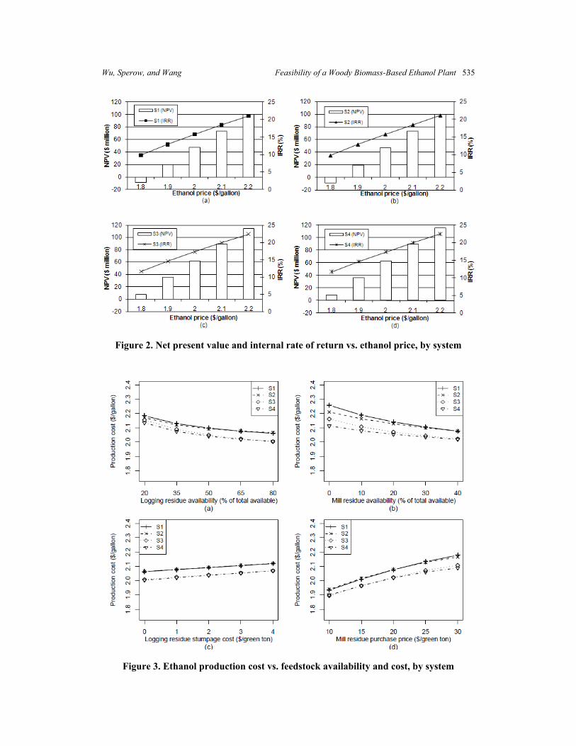
Ethanol price is critical to the evaluation of a cellulosic ethanol facility, and can have signifi-cant impacts on the NPV and IRR. The ethanol price is relatively volatile and subject to changes in the wholesale price of unleaded regular gasoline and additional volatility due to local, regional, and national supply and demand for ethanol (BBI International, 2002). The NPV and IRR were estimated in terms of various ethanol prices by different woody biomass handling systems (figure 2). The grapple skidder handling systems (S3 and S4) generated higher NPV and IRR than the cable skidder handling systems (S1 and S2). The magnitude of the NPV or IRR change was approximately proportional to the change of ethanol price for all systems. If ethanol price decreased $0.10 per gallon, the NPV of the base case plant (50 million gallons per year) over the plant life would decrease $27 million and the IRR would decrease 2.75%.

Ethanol Production Cost versus Feedstock Supply

Total feedstock was estimated at 3.61 million dry tons per year in West Virginia and some bordering counties (USDA/Forest Service, 2008). With the assumptions that 65% of logging residue on harvested sites with a slope of 35% or less and 40% of mill residue are available, the usable feedstock could be up to 1.87 million dry tons. Given the plant capacity of 2,000


Figure 2. Net present value and internal rate of return vs. ethanol price, by system

Figure 3. Ethanol production cost vs. feedstock availability and cost, by system

536 December 2010 Journal of Agricultural and Resource Economics dry tons per day in the base case, the feedstock needed annually is approximately 0.72 million dry tons, or 38.5% of the total available. Average ethanol production costs decreased as avail-able residue increased (figure 3a, b). There were significant differences among woody biomass handling systems in terms of ethanol production cost. The grapple skidder systems (S3 and S4) tended to have lower production cost compared to the cable skidder systems. Logging residue had greater impacts on ethanol production cost in contrast to mill residue because more logging residue could be delivered to the utilization facility. Ethanol production costs increased as stumpage costs of logging residue increased (figure 3c). For every $1 per ton increase in stumpage costs, production costs would increase $0.0140/gallon for the cable skidder-loose residue system (S1), $0.0143/gallon for the cable skidder chips system (S2), $0.0153/gallon for the grapple skidder-loose residue system (S3), and $0.0165/gallon for the grapple skidder-chips system (S4). If the purchase price of mill residue increased from $20/ton (base case) to $30/ton, the production cost would increase 3.4%–4.9% from the base case depending on the biomass handling system used (figure 3d).

Ethanol Production Cost versus Capital Cost

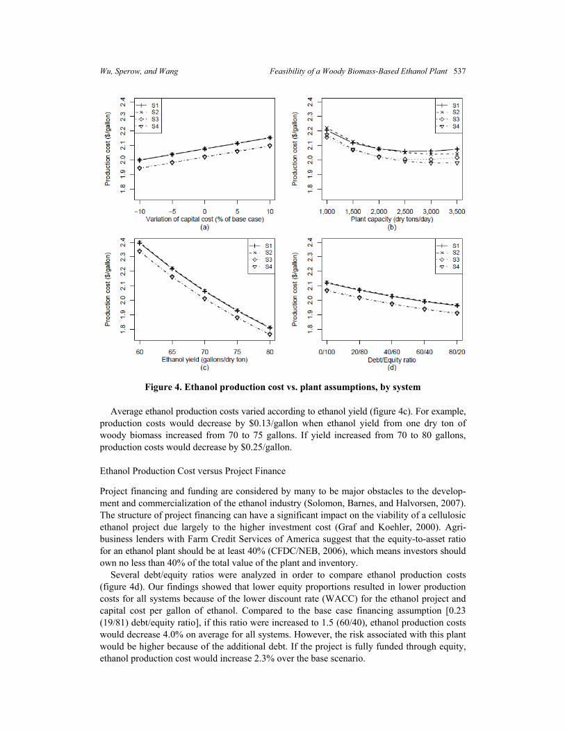
Ethanol production costs increased proportionally as total capital costs increased (figure 4a). If total capital costs increased 5% compared to the base case, the ethanol production costs would increase 1.8%–1.9%, depending on the biomass handling system used. Similarly, if the total capital cost increased 10%, the ethanol production cost would increase 3.7%–3.9% among the four handling systems.

Ethanol Production Cost versus Plant Capacity

Average ethanol production costs decreased as plant use of woody biomass increased (figure 4b). As plant scale increased, the average cost related to plant investment decreased due to economies of scale. However, the average cost associated with transportation increased because the plant had to source feedstock from a greater distance. Ethanol production costs reached the minimum when woody biomass use increased to 2,700 dry tons per day for S1 and S3, and 3,100 dry tons per day for S2 and S4. Therefore, the optimal plant size for the ethanol facility is 2,700 dry tons per day for S1 and S3, and 3,100 dry tons per day for S2 and S4. At the demand level of 2,700 dry tons per day, production costs in S1 and S3 decreased 0.98% compared to the base case. Production costs in S2 and S4 decreased 1.98% compared to the base case when plant capacity approached 3,100 dry tons per day. Production costs were always higher for cable skidder handling systems (S1 and S2) than grapple skidder handling systems (S3 and S4).

Ethanol Production Cost versus Ethanol Yield

Technologies that convert wood to cellulosic ethanol are in varying stages of development and commercialization (Benjamin, Lilieholm, and Damery, 2009). Ethanol yield from one dry ton of woody biomass could vary from 60 to 120 gallons depending on conversion technology and other operational conditions (Frontier Associates, LLC, 2008). The co-current dilute acid prehydrolysis and enzymatic hydrolysis developed by the National Renewable Energy Laboratory was considered as one of the available conversion methods, and the ethanol yield could be 68 gallons from one dry ton of woody biomass (Wooley et al., 1999).


Figure 4. Ethanol production cost vs. plant assumptions, by system Average ethanol production costs varied according to ethanol yield (figure 4c). For example, production costs would decrease by $0.13/gallon when ethanol yield from one dry ton of woody biomass increased from 70 to 75 gallons. If yield increased from 70 to 80 gallons, production costs would decrease by $0.25/gallon. Ethanol Production Cost versus Project Finance

Project financing and funding are considered by many to be major obstacles to the develop-ment and commercialization of the ethanol industry (Solomon, Barnes, and Halvorsen, 2007). The structure of project financing can have a significant impact on the viability of a cellulosic ethanol project due largely to the higher investment cost (Graf and Koehler, 2000). Agri-business lenders with Farm Credit Services of America suggest that the equity-to-asset ratio for an ethanol plant should be at least 40% (CFDC/NEB, 2006), which means investors should own no less than 40% of the total value of the plant and inventory. Several debt/equity ratios were analyzed in order to compare ethanol production costs (figure 4d). Our findings showed that lower equity proportions resulted in lower production costs for all systems because of the lower discount rate (WACC) for the ethanol project and capital cost per gallon of ethanol. Compared to the base case financing assumption [0.23 (19/81) debt/equity ratio], if this ratio were increased to 1.5 (60/40), ethanol production costs would decrease 4.0% on average for all systems. However, the risk associated with this plant would be higher because of the additional debt. If the project is fully funded through equity, ethanol production cost would increase 2.3% over the base scenario.

538 December 2010 Journal of Agricultural and Resource Economics Other Implications

Security of Feedstock Supply

Feedstock supply stabilization is critical to the success of a woody biomass-based facility. Increased regulation of forest practices, such as best management practices and certifications, often increases woody biomass harvesting costs and limits resource availability in the short term (Benjamin, Lilieholm, and Damery, 2009). Logging residue has been considered an under- utilized resource with limited value; however, more biomass would be needed and higher stumpage costs of logging residue would be inevitable as the biomass market develops for ethanol or other bioproducts. In considering the future availability of mill residue, several issues should be addressed. Since mill residue is a by-product of lumber production, its availability depends on other markets, as demonstrated recently by the corresponding decline in production of mill residue due to the housing slowdown (U.S. Census Bureau, 2009). The supply of mill residue in the central Appalachian region remains more uncertain because of mill closures and long-term production constraints (Dye, 2009). The utilization of woody biomass for biofuels will also challenge competition from other uses such as pellet fuel and boiler fuel, which could raise woody biomass prices. To secure the woody biomass supply chain, it is essential to find niche supply markets for wood residues through long-term contracts or collaborative relationships with landowners and major forest products companies. Government Policies

Government subsidies initially will be essential to the market success of woody biomass-based facilities. Without government subsidies, ethanol producers would have to sell their products at current market price. For example, in our case, the difference between the market price and the price used for this analysis could be $0.20 per gallon. Government and other support mechanisms have been a consistent and essential part of the U.S. ethanol industry (Solomon, Barnes, and Halvorsen, 2007). Various federal incentive programs have been designed to encourage the production and utilization of ethanol and other biofuels such as Excise Tax Incentives, Income Tax Credit for Alcohol Fuels, Ethanol Production Incentive, Income Tax Credit, Income Tax Credit for Small Ethanol Producers, and others. The most significant subsidy is the federal Volumetric Ethanol Excise Tax Credit (VEETC), which was established in 2004 as a $0.51 per gallon payment to gasoline blenders. As of January 1, 2009, the original tax credit on pure ethanol was reduced to $0.45 per gallon. The 2008 Farm Bill set the credit for cellulosic ethanol at $1.01 per gallon through 2012. At the current spot price of $1.88 per gallon (DTN Ethanol Center, 2009), the cellulosic ethanol plant in central Appalachia would not be economically viable without government subsidy. Ethanol Market

West Virginia is a moderate ethanol consumer with annual consumption of 542,620 barrels (22.79 million gallons). By comparison, Ohio, Virginia, and Pennsylvania consumed a total of approximately 11 million barrels of ethanol in 2005 (U.S. Department of Energy, 2009). Most ethanol consumed in this region is from the Midwest cornbelt. Due to the transport infrastructure bottleneck, ethanol availability is limited in the eastern states (Tyner, 2008). A


potential cellulose ethanol production of 50 million gallons in West Virginia could help meet the state’s own needs as well as supply markets in neighboring states. The business could also stimulate economic development and create job opportunities in urban and rural communities in the region.

Conclusions The economic model developed here can be used to assess the optimal location of a potential woody biomass-based ethanol facility in the central Appalachian region and to evaluate the economic viability under certain resource, capacity, and other constraints. This study differs from prior studies in several respects. First, the delivered cost of woody biomass was computed based on a series of logistic constraints including supply and demand. This cost would change as factors such as biomass availability, purchase price, and demand level at the ethanol plant changed. Second, the NPV was calculated in consideration of income taxes, while most previous studies only considered revenue and fixed and variable operating costs. By estimating the NPV using the mixed-integer programming model, an insight is gained into the economic viability of a cellulose ethanol facility. Third, the model can address optimizing logistical decision making when linked to feedstock requirements, collec-tion, delivery, and production issues. Because this is a generalized model, it also can be applied to other regions. The application results of the base case revealed that the optimal location for the woody biomass-based ethanol plant is in Buckhannon, West Virginia, which is surrounded by abundant woody biomass resources. The NPV varied from $68.11 million for the cable skidder-chips system (S2) to $84.51 million for the grapple skidder-chips system (S4) with an after-tax discount rate of 10.79% over the plant’s life. The real internal rate of return averaged 18.67% among the four woody biomass handling systems. The net cash flow of the plant became positive by the end of the fifth year. The primary revenue source of the facility came from the sale of ethanol and electricity, without considering the small ethanol producer tax credit. Ethanol production costs varied from $2.02 per gallon for the grapple skidder-chips system (S4) to $2.08 per gallon for the cable skidder-chips system (S2). Sivers and Zacchi (1996) reviewed the economy of ethanol production from lignocellulosic material and found high variation in ethanol production costs, from $0.68 to $5.71 per gallon. Wide variation in ethanol production cost can be explained by different assumptions made in the technical and economic calculations, such as raw materials used, the type of process utilized, and the design of the process. Sensitivity analyses indicated that ethanol production costs in the ethanol facility in the central Appalachian hardwood region depended heavily upon biomass availability, plant investment and capacity, ethanol yield, and financial structure. This study provides a solid base for further research in assessing the social and environ-mental issues of the woody biomass-based ethanol facility. Further efforts are necessary to assess the detailed plant configuration including equipment, utilities, and labor availability. Necessary permits related to air emissions and water pollution controls required for the ethanol facility in the designated location should be considered as well.

[Received October 2009; final revision received October 2010.]

540 December 2010 Journal of Agricultural and Resource Economics

References BBI International. “Feasibility Study for Bioethanol Co-Location with a Coal Fired Power Plant.” Res. Rep.

No. NREL/SR-510-32999, National Renewable Energy Laboratory, Golden, CO, 2002. Benjamin, J., R. J. Lilieholm, and D. Damery. “Challenges and Opportunities for the Northeastern Forest

Bioindustry.” J. Forestry 107,3(2009):125–131. Bragonje, R., S. Grushecky, B. Spong, J. Slahor, and L. Osborn. “West Virginia Wood By-products Avail-

able and Needed.” Appalachian Hardwood Center, West Virginia University, Morgantown, 2006. Bullis, K. Making Ethanol from Wood Chips. Technology published by MIT Review, 2006. Online.

Available at http://www.technologyreview.com/energy/17799/. Clean Fuels Development Coalition and Nebraska Ethanol Board. A Guide for Evaluating the Requirements

of Ethanol Plants, 2006. Online. Available at http://www.ne-ethanol.org/industry/evalreq.pdf. Cusack, C. “Harnessing the Power of Local Wood Energy,” 2008. Online. Available at http://www.forest

guild.org/publications/research/2008/Local_Wood_Energy.pdf. Deutscher, H. “Cellulosic Ethanol: Ready, Set, Go.” Ethanol Producer Magazine (July 2009):A9. Dornburg, V., and A. P. C. Faaij. “Efficiency and Economy of Wood-Fired Biomass Energy Systems in

Relation to Scale Regarding Heat and Power Generation Using Combustion and Gasification Tech-nologies.” Biomass and Bioenergy 21,2(2001):91–108.

DTN Ethanol Center. “Weekly Ethanol Rack Prices.” Online. Available at http://www.dtnethanolcenter.com/ index.cfm?show=10&mid=32. [Accessed July 28, 2009.]

Dye, R. “Challenging Times.” Paper presented at the 23rd Annual A. B. Brooks Forestry Symposium, Charleston, WV, 6–7 February 2009.

Faqs.org. Verenium Corp.–Form 10-K–March 15, 2010. Online. Available at http://www.faqs.org/sec-filings/ 100316/VERENIUM-CORP_10-K/. [Accessed July 2010.]

Fehrenbacher, K. “Verenium Opens Cellulosic Ethanol Demo Plant.” 28 May 2008. Online. Available at http://earth2tech.com/2008/05/28/verenium-opens-cellulosic-ethanol-demo-plant/.

Frontier Associates, LLC. “Texas Renewable Energy Resource Assessment.” Texas State Energy Office, Austin, TX, 2008.

Graf, A., and T. Koehler. “Oregon Cellulose-Ethanol Study—An Evaluation of the Potential for Ethanol Production in Oregon Using Cellulose-Based Feedstocks.” Oregon Office of Energy, 2000. Online. Available at http://www.ethanol-gec.org/information/briefing/20a.pdf.

Graham, R. L., B. C. English, and C. E. Noon. “A Geographical Information System-Based Modeling System for Evaluating the Cost of Delivered Energy Crop Feedstock.” Biomass and Bioenergy 18,4(2000):309–329.

Greer, D. “Realities, Opportunities for Cellulose Ethanol.” Biocycle 48,1(2007):46. Grushecky, S., D. McGill, and R. B. Anderson. “Inventory of Wood Residues in Southern West Virginia.”

No. J. Appl. Forestry 23,1(2006):47–52. Illinois Environmental Protection Agency and Illinois Department of Commerce and Economic Opportunity.

Building an Ethanol Plant in Illinois—A Guide to Permit Requirements, Funding Opportunities, and Other Considerations. The State of Illinois, 2006. Online. Available at http://www.epa.state.il.us/agriculture/ building-an-ethanol-plant.pdf.

InflationData.com. Historical Inflation Rate. Online. Available at http://www.inflationdata.com/inflation/ inflation/inflation.asp. [Accessed July 2010.]

iStockAnalyst. Historical Annual Returns for the S&P 500 Index. Online. Available at http://www.istock analyst.com/article/viewarticle/articleid/2803347. [Accessed July 2010.]

Kärhä, K., and T. Vartiamäki. “Productivity and Costs of Slash Bundling in Nordic Conditions.” Biomass and Bioenergy 30,12(2006):1043–1052.

Kaylen, M., D. L. Vandyne, Y. S. Choi, and M. Blase. “Economic Feasibility of Producing Ethanol from Lignocellulosic Feedstocks.” Bioresource Technology 72,1(2000):19–32.

Kerstetter, J. D., and J. K. Lyons. “Logging and Agricultural Residue Supply Curves for the Pacific Northwest.” Agreement No. DE-FC01-99EE50616, U.S. Department of Energy, Washington, DC, January 2001.

Li, Y., J. Wang, G. Miller, and J. McNeel. “Production Economics of Harvesting Small-Diameter Hardwood Stands in Central Appalachia.” Forest Products J. 56,3(2006):81–86.


Mapemba, D., F. M. Epplin, R. L. Huhnke, and C. M. Taliaferro. “Herbaceous Plant Biomass Harvest and

Delivery Cost with Harvest Segmented by Month and Number of Harvest Machines Endogenously Determined.” Biomass and Bioenergy 32(2008):1016–1027.

Mapemba, L. D., F. M. Epplin, C. M. Taliaferro, and R. L. Huhnke. “Biorefinery Feedstock Production on Conservation Reserve Program Land.” Rev. Agr. Econ. 29,2(2007):227–246.

McMenamin, J. Financial Management. London: Routledge, 1999. Miyata, E. S. “Determining Fixed and Operating Costs of Logging Equipment.” General Tech. Rep. No. NC-

55, USDA/Forest Service, 1980. MyRatePlan.com. Distance Calculator—How Far Is It Between Two Cities? Online. Available at http://www.

myrateplan.com/how_far/. [Accessed May 2008.] Nienow, S., K. T. McNamara, and A. R. Gillespie. “Assessing Plantation Biomass for Co-firing with Coal in

Northern Indiana: A Linear Programming Approach.” Biomass and Bioenergy 18(2000):125–135. Nienow, S., K. T. McNamara, A. R. Gillespie, and P. V. Preckel. “A Model for the Economic Evaluation of

Plantation Biomass Production for Co-firing with Coal in Electricity Production.” Agr. and Resour. Econ. Rev. 28(1999):106–118.

Noon, C. E., F. B. Zhan, and R. L. Graham. “GIS-Based Analysis of Marginal Price Variation with an Appli-cation in the Identification of Candidate Ethanol Conversion Plant Locations.” Networks and Spatial Econ. 2,1(2002):79–93.

Perlack, R. D., L. L. Wright, A. F. Turhollow, R. L. Graham, B. J. Stokes, and D. C. Erbach. “Biomass as Feedstock for a Bioenergy and Bioproducts Industry: The Technical Feasibility of a Billion-Ton Annual Supply.” U.S. Department of Energy and U.S. Department of Agriculture, Washington, DC, 2005.

Short, W., D. J. Packey, and T. Holt. “A Manual for the Economic Evaluation and Energy Efficiency and Renewable Energy Technologies.” Res. Rep. No. TP-462-5173, National Renewable Energy Laboratory, Golden, CO, 1995.

Sivers, M. V., and G. Zacchi. “Ethanol from Lignocellulosics: A Review of the Economy.” Bioresource Technology 56,2(1996):131–140.

Solomon, B. D., J. R. Barnes, and K. E. Halvorsen. “Grain and Cellulosic Ethanol: History, Economics, and Energy Policy.” Biomass and Bioenergy 31(2007):416–425.

Taha, H. A. Operations Research: An Introduction, 8th ed. Englewood Cliffs, NJ: Pearson Prentice-Hall, 2006.

Taheripour, F., and W. E. Tyner. “Ethanol Policy Analysis—What Have We Learned So Far?” Choices (3rd Quarter 2008):6–11.

Tembo, G., F. Epplin, and R. R. Huhnke. “Integrative Investment Appraisal of a Lignocellulosic Biomass-to-Ethanol Industry.” J. Agr. and Resour. Econ. 28,3(December 2003):611–633.

Tyner, W. E. “The U.S. Ethanol and Biofuels Boom: Its Origins, Current Status, and Future Prospects.” Bioscience 58,7(2008):646–653.

Tyner, W. E., and F. Taheripour. “Future Biofuels Policy Alternatives.” In Proceedings of Biofuels, Food & Feed Tradeoffs [held 12–13 April 2007], eds., J. L. Outlaw, J. A. Duffield, and D. P. Ernstes, pp. 10–18. Farm Foundation, Oak Brook, IL, 2007.

Ulrich, G. D. A Guide to Chemical Engineering Process Design and Economics. New York: Wiley, 1984. U.S. Census Bureau. Lumber Production and Mill Stocks—2008 Annual. Pub. No. MA321T(08)-1, Wash-

ington, DC. Online. Available at http://www.census.gov/cir/www/321/ma321t.html. [Accessed January 2009.]

U.S. Department of Agriculture, Forest Service. Timber Products Output Mapmaker, Version 1.0. Online. Available at http://ncrs2.fs.fed.us/4801/fiadb/rpa_tpo/wc_rpa_tpo.ASP. [Accessed May 2008.]

U.S. Department of Energy. State Energy Summary. Online. Available at http://apps1.eere.energy.gov/ states/state_information.cfm. [Accessed March 2009.]

U.S. Department of State. “West Virginia Weather.” Online. Available at http://countrystudies.us/united-states/weather/west-virginia/. [Accessed June 2009.]

U.S. Department of the Treasury. “Daily Treasury Yield Curve Rates.” Online. Available at http://www. ustreas.gov/offices/domestic-finance/debt-management/interest-rate/yield.shtml. [Accessed July 2010.]

U.S. Environmental Protection Agency. “Renewable Fuel Standard Program (RFS2) Regulatory Impact Analysis.” Online. Available at http://nepis.epa.gov/Adobe/PDF/P1006DXP.PDF. [Accessed May 2010.]

542 December 2010 Journal of Agricultural and Resource Economics Van Horne, J. C. Financial Management and Policy, 6th ed. Englewood Cliffs, NJ: Prentice-Hall, 1984. Volker, R., H. Schaaf, and P. Tachkov. “Evaluation of Research and Technology Projects: A Status Quo

Analysis of Technology-Intensive Companies.” Internat. J. Technology Intelligence and Planning 5,2(2009):165–190.

Wang, J., S. Grushecky, and J. McNeel. “Biomass Resources, Uses, and Opportunities in West Virginia.” Biomaterials Center, West Virginia University, Morgantown, 2006.

Wang, J., C. Long, and J. McNeel. “Production and Cost Analysis of a Feller-Buncher and Grapple Skidder in Central Appalachian Hardwood Forests.” Forest Products J. 54,12(2004):159–167.

West Virginia Division of Forestry. “West Virginia Logging Sediment Control Act—2006 Statistics.” West Virginia Division of Forestry, Charleston, 2006.

Wooley, R., M. Ruth, J. Sheehan, K. Ibsen, H. Majdeski, and A. Galvez. “Lignocellulosic Biomass-to-Ethanol Process Design and Economics Utilizing Co-current Dilute Acid Prehydrolysis and Enzymatic Hydrolysis Current and Futuristic Scenarios.” Res. Rep. No. NREL/TP-580-26157, National Renewable Energy Laboratory, Golden, CO, 1999.

Wu, J., J. Wang, and J. McNeel. “Economic Modeling of Woody Biomass Utilization for Biofuels: A Case Study in West Virginia.” In Proceedings of the 31st Annual Meeting of the Council on Forest Engi-neering (held 22–25 June 2008), pp. 206–218. Charleston, WV: Council on Forest Engineering, 2008.

Zerbe, J. I. “Liquid Fuels from Wood-Ethanol, Methanol, Diesel.” World Resour. Rev. 3,4(1991):406–414.

Appendix: Sets, Parameters, and Variables Used in the Model

Table A1. Sets and Descriptions

Set Description

G Products; g = {ethanol, electricity }

H Woody biomass handling systems; h = {1, 2, 3, 4}, where 1 = cable skidder loose residue, 2 = cable skidder chips, 3 = grapple skidder loose residue, and 4 = grapple skidder chips

I Woody biomass supply locations; i = {all counties in West Virginia and some counties in the bordering states}

J Possible plant locations; j = {Beaver, Belington, Bluefield, Buckhannon, Holden, Kenna, Millwood, Morgantown, Oak Hill, Point Pleasant, and Williamson}

K Facility type; k = {general_plant, steam_plant}

M Months; m = {1 , 2, ..., 12}

T Set of project year indices; t = {1 , 2, ..., T}

S Set of breakpoints; s = {0, 1, ..., 9}

Table A2. Parameters and Descriptions

Parameter Description

as Breakpoints over the quantity of annually delivered logging residue from supply county i to plant j

ALFAih A parameter associated with system h at supply location i, ALFAih = {0, 1}

BPi Proportion of logging residue available for extraction at supply location i (%)

BIVi Volume of logging residue at supply location i (green tons)

BVSi Volume of logging residue on forest lands with a slope of 35% or less at supply location i (green tons)

Ct Capital depreciations at the tth year ($)

CFkt Depreciation cost of facility type k at the tth year ($)

CFDkt Declining balance depreciation cost of facility type k at the tth year ($)

( continued . . . )


Table A2. Continued


CFSkt Straight line depreciation cost of facility type k at the tth year ($)

CRkt Unrecovered capital cost of facility type k at the tth year ($)

CSh In-woods chipping cost associated with handling system h ($/green ton)

CPh Chipping cost at a plant associated with system h ($/green ton)

CAPACITY Plant capacity in terms of woody biomass required (dry tons/day)

CAPACITY0 Production capacity of a known woody biomass-based plant (dry tons/day)

D Market value of the firm’s debt ($)

DISij One-way over-the-road distance between supply location i to plant j (miles)

E Market value of the firm’s equity ($)

EXTm Limitation of logging residue extracted in month m as a percentage of the whole year (%)

FCs Slope of the sth line segment in the range (as−1 , as)

HCh Logging residue extraction cost for handling system h ($/green ton)

INTt Principal and interest payment at the tth year ($)

LCh Loading cost of woody biomass associated with system h ($/green ton)

MC Purchase price of mill residue ($/green ton)

MT Mill residue transportation cost rate ($/ton/mile)

MIVi Volume of mill residue at supply location i (green tons)

MPi Mill residue availability at supply location i (%)

MS Marshall & Swift index in the initial project year

MS0 Marshall & Swift index in the historical year

MNBIN Minimum biomass inventory at a plant (green tons)

NRk Recovery period of facility type k (years)

NLi Number of loggers in supply location i

NMh Average number of extraction machines that a logging crew owns

OMt Operation and maintenance costs at the tth year ($)

Pg Wholesale price per unit of product g ($/gallon for ethanol and $/kWh for electricity)

PDh Productivity of extraction machine associated with system h (green tons/hour)

PVIt Present value of $1 at the tth year ($)

re Real cost of equity (%)

rd Real cost of debt (%)

RSi One-half of the farthest straight-line distance (e.g., distance from the east to north) of supply county i (miles)

SC Logging residue storage cost at landings ($/green ton)

SP Stumpage price of logging residue ($/green ton)

τ Federal tax rate applied to the ethanol facility (%)

TCijh Round-trip transportation cost from location i to plant j for system h ($/green ton)

ς h Off-highway transportation cost rate for system h ($/ton/mile)

TPCj Plant investment cost at location j ($); TPCj = TPC j

TPC0 Investment cost of a known woody biomass-based ethanol plant ($)

we Equity proportion of the project (%)

WACC Weighted average cost of capital (%)

σ Moisture content of woody biomass (%)

( continued . . . )

544 December 2010 Journal of Agricultural and Resource Economics Table A2. Continued


ηg Conversion factor for product g from one dry metric ton of woody biomass

λ Monthly productive time per machine (hours)

δ Dry matter loss due to woody biomass transportation (%)

θ i Usable proportion of woody biomass in the fields at location i (%)

Usable proportion of woody biomass at a plant (%)

ε Scheduled working days per month

Table A3. Variables and Descriptions

Variable Description

β j A binary variable associated with plant j; β j = {0, 1}

qjgm Quantity of product g produced in month m at plant location j

Ft Annual feedstock cost ($)

LCT Underestimated transportation cost ($)

Rt Annual revenue from the sale of products ($)

TXt Income taxes at the tth year ($)

NPV Net present value of the plant ($)

xhihm Quantity of logging residue extracted in month m at supply location i using system h (green tons)

xmijm Quantity of mill residue delivered from supply location i to plant j in month m (green tons)

xppjm Quantity of woody biomass processed at plant j in month m (green tons)

xpsihm Quantity of logging residue entered into storage at supply location i in month m associated with system h (green tons)

xsihm Quantity of logging residue stored at location i in month m associated with system h (green tons)

xsnihm Quantity of logging residue removed from storage at location i in month m associated with system h (green tons)

xssjm Quantity of woody biomass stored at plant j in month m (green tons)

xtijhm Quantity of logging residue delivered from supply location i to plant j in month m associated with system h (green tons)

xtlijhs The increment of logging residue annually shipped out of supply location i in the range (as−1, as) (green tons)

Economic Feasibility of a Woody Biomass- Based Ethanol ... · Economic Feasibility of a Woody...

Documents

Transcript of Economic Feasibility of a Woody Biomass- Based Ethanol ... · Economic Feasibility of a Woody...