Economic Evaluation of Investment Projects Under...

1

Ref. No: SCI-1801-1599

Economic Evaluation of Investment Projects Under

Uncertainty: A Probability Theory Perspective

Hadi Mokhtari *, Saba Kiani, Seyed Saman Tahmasebpoor

Department of Industrial Engineering, Faculty of Engineering, University of Kashan, Kashan, Iran Hadi Mokhtari

Postal code: 8731753153, Tel.: +98 031 55912476, email: [email protected]

Saba Kiani

Postal code: 8731753153, Tel.: +98 031 55912476, email: [email protected]

Seyed Saman Tahmasebpoor Postal code: 8731753153, Tel.: +98 031 55912476, email: [email protected]

Abstract. In the current competitive economy, the investors are facing

increased uncertainty while evaluating new investment projects. This

uncertainty caused from existence of insufficient information, oscillating

markets, unstable economic conditions, obsolescence of technology and so on,

and hence uncertainty is inevitable in reality. In such conditions, the

deterministic models, while easy to use, do not perfectly represent the real

situations and might lead to misleading decisions. When the cash flows for an

uncertain investment project, over a number of future periods, are discounted

using the traditional deterministic approaches, it may not provide investors

with an accurate estimation of the project value. Therefore, this paper utilizes

2

the probability theory tools to derive closed-form probability distribution

function (PDF) and related expressions of the net present worth (NPW), as a

useful and frequently used criterion, for cost-benefit evaluation of projects.

The random cash flows follow normal, uniform or exponential distributions in

our analysis. The probability distribution function of the NPW is an important

tool that helps investors to accurately estimate the probability of being

economic for projects, and hence, it is important tool for investment decision-

making under uncertainty.

Keywords: Investment Projects; Economic Evaluation; Net Present Worth;

Probability Distributions; Probability Theory

1.‌ Introduction

Appropriate evaluation and selection of investment projects is the most important

financial factor for success of investors and is vital to be economic in current

competitive environment [1]. The investors aim to not only prevent projects'

failures, but also select the best alternatives among available investment projects

so as to gain more benefits and reach better results. In the economic evaluation of

investment projects, the important parameters such as prices and quantities have

been treated so far based on the deterministic and pre-known values. The values of

these parameters used in the analysis and the resulting outcomes are single values

with perfect certainty. An investor expects to achieve positive results from an

investment projects. Under deterministic settings, these results can be determined

unambiguously. However, under uncertainty in the real-world conditions, there

are usually lack of reliable information [2], and most investment parameters are

uncertain [3]. The future outcomes have uncertainties especially for long-term

planning horizons and variability in the value of future items is inevitable. In real-

world, uncertainty is always present and, in some especial cases, due to lack of

scientific information and existence of technological innovation, it is more difficult

to make reliable decisions. For example, the new products supplied to market

might not gain sales at the expected levels; the profits expected from international

investments might not be gained satisfactorily; or an investment might have

unexpectedly delay to a long time to achieve efficiency. The source of this

3

uncertainty might be the behaviors of customers, suppliers or employees, or

technical problems in processes. Due to complex and fast-changing factors in

decision making, many investment decisions contain remarkable uncertainty and,

hence, suffer high risks in outcomes. Therefore, these uncertainties should be take

into account in economic evaluation of investment projects, in order to ensure

reliable decisions and long-term achievements.

The cash flow analysis has been utilized to assess the differences among

investment projects and to provide a basis for project evaluation. In order to

financially evaluate investment projects, it is needed to assess beneficiary due to

their cash flows. In evaluation of investment projects, the cash flow analysis is

carried out by the classic methods like net present worth (NPW), net future worth

(NFW), net equivalent uniform annual (NEUA), internal rate of return

(ROR/IRR), payback period (PB) and etc. Among them, the NPW is one of the

most useful one for finding the economic desirability of the projects. The

appropriate criterion for monitoring and evaluating such projects is NPW [4-5]. It

is considered to be a major tool for analyzing the cash flow of projects during a

long period [6]. It is the most common methods used by banks and large-sized

organizations to compare projects select most economic among them. To perform

such analysis, the NPW of an investment project is defined as sum of present

income cash flow minus present cost cash flow during the project's time horizon.

Hence, NPW criterion can be calculated via:

1 1

nt t

t

t

R CNPW

i

(1)

where tr and tc indicate the value of income and cost during the period t

respectively, i indicates the discount rate (minimum attractive rate of return), and

n indicates the project's planning horizon. If the value of NPW is equal or bigger

than zero, the project will be economic and acceptable, and if it is smaller than

zero, the project will be uneconomic and hence unacceptable. To incorporate NPW

in uncertain environment, different approaches have been used in literature. The

most used methods are based on soft computing approaches like Fuzzy sets and

simulation [2]. The fuzzy mathematical optimization [7], the fuzzy data

envelopment analysis [8], and the fuzzy AHP and ANP [9] have attracted most

attentions. Moreover, different hybrid approaches [9-10] tries to combine these

methods to reach better results. As another frequently used approach, the

4

simulation has been utilized in different ways. Some researchers have used

simulation tool incorporated with the transformation of fuzzy numbers to

probability distributions [4], others utilized Monte-Carlo simulation to achieve

sample sizes [11] and others have used fuzzy simulation directly [12]. Naimi

Sadigh et al., [13] proposed a hybrid approach based on particle swarm

optimization and Hopfield neural network to a cardinality constrained portfolio

optimization problem. Salmasnia et al., [14] proposed a robust approach to

project evaluation with time, cost, and quality considerations. Liu and Wu [15]

presented a portfolio evaluation and optimization in electricity markets. Afshar-

Nadjafi et al., [16] proposed a generalized resource investment problem with

discounted cash flows and progress payment. Rębiasz and Macioł [17] employed a

multi-criteria decision making methods and a fuzzy rule-based approach for

investment projects evaluation. Dai et al., [18] discussed a model for renewable

energy investment project evaluation based on improved real option approach.

Kilic and Kaya [19] investigated a decision making methodology for an investment

project evaluation by based on type-II fuzzy sets. Kirkwood et al. [20] evaluated

uncertainty in an integrated maintenance of the UK rail industry by net present

value calculations. Tabrizi et al., [21] a novel project portfolio selection by using a

fuzzy DEMATEL and goal programming. Fathallahi and Naja [22] designed a

hybrid genetic algorithm to maximize net present value of fuzzy project cash flows

in resource-constrained project scheduling problem. In addition, Dutta and

Ashtekar [23] considered a system dynamics simulation tool for project evaluation

issue. Etemadi, et al., [24] A goal programming capital budgeting model under

uncertainty in construction industry. Mohagheghi et al., [25] suggested a new

interval type-II fuzzy optimization approach for R&D project evaluation and

portfolio selection. Awasthi and Omrani [26] developed a scenario simulation

approach for sustainable project evaluation based on fuzzy concepts.

All above soft methods can be applied if essential assumptions such as existence of

large sample and data accuracy are assured. However, another useful approach to

handle uncertainty in economic evaluation is estimating some prediction functions

like probability distribution function (PDF). It is an analytical approach, in

contrast to soft approaches, to evaluate investment projects based on the

probability and statistical theory principles. In this way, the probability

distribution functions (PDFs) for estimation and prediction of economic

5

desirability MPW can be derived [27]. In this paper, we propose to derive the

probability distribution function of economic desirability NPW for two classes of

investment projects: (i) one-period cash flows (three cases), and (ii) two-period

cash flows (six cases). In deterministic environment, under certainty, a project is

evaluated as "economic" or "uneconomic". However, in stochastic environment,

under uncertainty, we can just talk about the "probability of being economic" or "

probability of being uneconomic" which can be calculated using the analytical PDF

of performance criterion NPW. In deterministic economic evaluation problems,

the investor has his/her own minimum attractive rate of return (MARR) which is

used in his/her evaluations. In our stochastic problems, we calculate the

probability of being economic for an uncertain cash flow. When this parameter is

calculated, the investor compares this parameter with his/her minimum

probability of being economic. If the minimum probability of being economic is

satisfied, the project is selected as economic, and otherwise, it is rejected. Hence,

this paper helps the investor to achieve the analytical function for estimating the

economic performance of investment projects. The probability theory tools like

moment generating function (MGF) and transformation method will be used, to

derive the analytical and closed-form function for probability distribution function

(PDF) of the net present worth (NPW) in investment projects. This analysis will be

performed for three classes of investment projects: (i) one-period cash flows, (ii)

two-period cash flows and (iii) multiple period cash flows, all with normal,

exponential and uniform distributions of cash flows. The probability distribution

functions of NPW will be derived for each cases separately, which can helps

investors to accurately estimate the economic desirability of investment projects

under uncertain cash flows. Since the cash flows follow continuous numbers, we

should consider continuous random distribution functions. For this purpose, we

consider normal, exponential and uniform distributions as well-known and most

frequently used continuous distributions for addressing random cash flows.

The rest of this paper is organized as follows. Section 2 provides one-period cash

flow analysis, while Section 3 discussed two-period cash flow analysis and Section

4 investigated a multiple-period project cash flow under uncertainty. In Sections

2-4, the probability distribution functions are derived for NPW in three

distributions, i.e., Normal, Exponential and Uniform, separately. Moreover, some

lemmas are proved to address the special cases of PDFs. Section 5 presents the

6

analysis and simulation results to evaluate the performance of PDFs derived and

calculate the probability of being economic for case examples in different

situations. Finally, Section 6 concludes the paper and suggests some directions for

future studies.

2. One-Period Cash Flow Analysis

This section introduces and investigates an investment problem consisting of a

one-period project with an initial cost 0A and an income at the end of the period 1 A

. The value of income 1A is usually bigger than that of cost 0A , but at continue, our

analysis let 1A to be smaller than 0A . The economic desirability of this project

NPW is a function of both cash flows 1A and 0A , which can be calculated as

follows:

1

01

ANPW A

i

(2)

If the income 1A is random, the economic desirability NPW will be random too,

and the mean and the variance of economic desirability NPW can be calculated as

follows:

1 1

2

0 2,

1 1

A AE NPW A Var NPW

i i

(3)

where1

A and 1

2

A indicate, respectively, the mean and the variance of the random

income 1A .

2.1. Fixed Cost 0A and Variable Income 1 A with Normal Distribution

In this case, by taking into account the assumptions 2

0 1 1 10, ~ , A A Normal , it

can be concluded that the economic desirability of project NPW is also a random

variable, with mean and variance as follows:

2

1 10 2

, 1 1

E NPW A Var NPWi i

(4)

7

So according to the normal distribution, probability distribution function ( PDF )

of income 1 A can be calculated as follows:

1

2

1 1

1 1 2

11

1:

22A

aPDF A f a EXP

(5)

And also its moment generating function ( MGF ) can be calculated as follows:

1

22

1 1 12

A

tMGF t E EXP tA EXP t

(6)

By considering the fact that the economic desirability of this project NPW is a

function of variable 1 A , the moment generating function of NPW can be therefore

calculated as follows:

1

01

NPW AA

i

MGF t MGF t

(7)

According to the knowledge of probability theory, it has been proved for one

random variable like Y and two fixed numbers like a and b that:

.aY b Y

tMGF t EXP bt MGF

a

(8)

Therefore, by using the above equation, moment generating function of economic

desirability of this project NPWMGF t is obtained as follows:

10 .

1NPW A

tMGF t EXP A t MGF

i

(9)

By substituting the moment generating function of income 1A in the above

equation, the NPWMGF t can be re-written as follows:

22

1 10

1 2 1NPW

tMGF t EXP t A

i i

(10)

By comparing the above NPWMGF t to the moment generating function of the

normal distribution, and by using the fact that moment generating function is

unique for every random variable, it can be concluded that:

2

1 10~ ,

1 1NPW Normal A

i i

(11)

8

Therefore, the probability distribution function of the economic desirability of this

project NPW is estimated as follows:

2

1 0

2

11

1 11:

22NPW

v i A iiPDF NPW f v EXP

(12)

The importance of this function is that it can help the investors to estimate the

economic desirability of such projects by calculating the probability of being

economic. When the minimum attractive rate of return (MARR) of investor is i ,

this probability can be calculated as follows:

0 1

1

1( 0 | ) 1

A iP NPW i

(13)

where . indicates the cumulative distribution function (CDF ) of the standard

normal distribution. Obviously, the projects with higher value of ( 0 | )P NPW i

are more economic and preferable.

2.2. Fixed Cost 0 A and Variable Income 1 A with Exponential

Distribution

In this case, by taking into account the assumptions 0 1 10, ~ A A EXP , the mean

and the variance of income 1A are 1 1E A and 2

1 1Var A , and consequently

the mean and the variance of the economic desirability of project NPW can be


2

1 10 2

, 1 1

E NPW A Var NPWi i

(14)

In addition, the probability distribution function of the income 1A , according to the

probability distribution function of the exponential random variable, is obtained

as follows:

1

11 1

1 1

1: A

aPDF A f a EXP

(15)

And the moment generating function of the income 1A is achieved as follows:

9

1 1

1

1

1AMGF t E EXP tA

t

(16)

By considering the fact that the economic desirability of the project NPW is a

function of random variable 1A , so by using the equation (9), moment generating

function of the economic desirability NPW can be derived as follows:

0

1

1

1NPW

iMGF t EXP A t

i t

(17)

Since this function does not adopt to any of the known random variables, so it can

be understood that the economic desirability of such project does not have a

standard pattern. But for the purpose of economic evaluation, we are looking for

this unknown pattern. So we use another probability theory analysis, i.e.,

transformation method in sequel [28]. To adopt this method, the reverse function

of economic desirability 1NPW is calculated as follows:

1

1 0: 1NPW A NPW A i (18)

And also derivative of the reverse function is calculated as '

1 1NPW i . So

according to the transformation method, the probability distribution function of

the economic desirability of project can be extracted as follows:

1

'1 1: .NPW APDF NPW f v f NPW NPW (19)

After the mathematical simplification, the above probability distribution function

NPWf v can be re-written in its final form as follows:

0

1 1

11: NPW

v A iiPDF NPW f v EXP

(20)

According to this, it can be concluded that if the income 1A has its least amount

which is zero, economic desirability of project NPW will be in its least amount

which is – 0A . It means that the range of NPW variations is as follows:

0A NPW (21)

Therefore, the condition of being economic for such a project, when investor have

a particular minimum attractive rate of return i , can be calculated as follows:

10

0

( 0 | ) NPWP NPW i f v dv

(22)

This probability is calculated and re-written as follows:

0

1

1( 0 | )

A iP NPW i EXP

(23)

By using the above equation, investors can easily predict the economic desirability

of such projects and take the appropriate economic decision.

2.3. Fixed Cost 0A and Variable Income 1A with Uniform Distribution

In this case, it has been assumed that 0 1 1 1 0, ~ , A A Uniform and, then the mean

and the variance of income 1A can be calculated as follow:

2

1 11 11 1,

2 12E A Var A

(24)

Therefore, the mean and the variance of the economic desirability of project NPW

is achieved as follows:

2

1 1 1 10

1 1,

2 1 12 1E NPW A Var NPW

i i

(25)

Moreover, the probability distribution function of the income 1A can be attained as

follows:

11 1 1 1 1

1 1

1: , APDF A f a a

(26)

And the moment generating function of the income 1A can be computed by:

1

1 1

1

1 1

A

EXP t EXP tMGF t E EXP tA

t

(27)

So, by using the equation (9), the moment generating function of the economic

desirability of the project NPW is gained as:

1 10 0

1 1

1 1

1 1

NPW

EXP t A EXP t Ai i

MGF t

ti i

(28)

11

By comparing the above NPWMGF t to the moment generating function of the

uniform distribution, and by considering the fact that the moment generating

function is unique for every random variable, it is revealed that:

1 10 0 ~ ,

1 1NPW Uniform A A

i i

(29)

and the probability distribution function of the economic desirability of this

project is estimated as follows:

1 10 0

1 1

1: ,

1 1NPW

iPDF NPW f v A v A

i i

(30)

Consequently, the probability of being economic for such projects, when investor

have a particular maximum attractive rate of return i , is calculated as follows:

0


(31)

This probability can be calculated and re-written as follows:

1 0

1 1

1( 0 | )

A iP NPW i

(32)

Further analysis of above equation reveals that it is not valid for two special cases

and it requires more investigation. For this purpose, two lemmas are presented

and discussed in sequel.

Lemma 1: In a one-period project with a fixed cost 0A and a variable income 1A

which follows uniform distribution 1 1 1 ~ , A Uniform , if 1 0 1A i , then we can

conclude that this project is certainly uneconomic.

Proof: If the assumption of this lemma is true, it can be concluded that

10 0

1A

i

and by using the fact 1 1 , it yields that 1

0 01

Ai

. So, both the

upper bound and the lower bound of NPW are negative and there is no chance for

the economic viability of this project. We can represent the result of this lemma in

mathematical form as given below:

1 0( 0 | ) 0 if 1P NPW i A i (33)

12

Lemma 2: In a one-period project with a fixed cost 0A and a variable income 1A

which follows uniform distribution 1 1 1 ~ , ,A Uniform if 1 0 1 ,A i then we can

conclude that the project is certainly economic.

Proof: If the assumption of this lemma is true, it can be concluded that

10 0

1A

i

and by using the fact 1 1 , it yields that 1

0 01

Ai

. So both the

upper bound and the lower bound of the NPW are positive and the economic this

project is economic certainly. It means:

1 0( 0 | ) 1 if 1P NPW i A i (34)

So according to both Lemmas 1 and 2, the probability of being economic for such

projects is re-written in general form as follows:

( 0 | )P NPW i (35)

1 0

1 0

1 0 1 0

1 1

1 0

0 1

1 1 & 1

1 1

if A i

A iif A i A i

if A i

By using the above equation, the economic desirability of such project can be

simply estimated.

The aim of this section was to determine the probability of being economic for

investment projects with one-period cash flow through deriving the analytical

equation of the NPW distribution function. For this purpose, three cases were

analyzed. These cases are applicable in reality where the cost parameter 0A was a

fixed positive number and income 1A was a random variable with three distinct

cases: (i) normal, (ii) exponential, and (iii) uniform distributions. For all of cases,

analytical PDF of NPW were derived mathematically, which are useful tools for

investors in evaluation of uncertain projects over one period cash flow.

3. Two-Period Cash Flow Analysis

13

This section investigates an investment problem consisting of a two-period project

with an initial cost 0A , an income at the end of first period 1A , and another income

at the end of second period 2A . In this project, the economic desirability NPW is a

function of 0 A , 1A and 2A cash flows, which can be calculated as follows:

1 2

0 21 1

A ANPW A

i i

(36)

By taking into account the assumptions that incomes 1A and 2A are random and

independent variables, the economic desirability NPW will be therefore random

with the mean and the variance as follows:

1 2 1 1

2 2

0 2 2 4,

1 1 1 1

A A A AE NPW A Var NPW

i i i i

(37)

where 1A and

1

2

A indicate the mean and variance of first random income 1A

respectively, and 2A and

1

2

A indicate the mean and variance of second random

income 2A . The aim is to determine the economic desirability of such project

through the determination of analytical equation for the probability distribution

function of NPW. To this end, six cases are analyzed in sequel. In all of these cases,

initial cost 0A is a fixed positive number and incomes 1A or 2 A are random

variables with (i) normal, (ii) exponential, and (iii) uniform distributions.

3.1. Fixed Cost 0A , Fixed Income 1 A , and Variable Income 2 A with

Normal Distribution

In this case, by considering the assumptions 0 10, 0, A A and 2

2 2 2~ , A Normal ,

it can be concluded that economic desirability of such project NPW is also

variable, and then the mean and variance of NPW can be calculated as follows:

2

1 2 20 2 4

, 1 1 1

AE NPW A Var NPW

i i i

(38)

Moreover, the moment generating function of income 2A can be calculated as:

2

22

2 2 22

A

tMGF t E EXP tA EXP t

(39)

14

and the moment generating function of NPW is a function of variable income 2A as

given below:

1 2

0 21 1

NPWA A

Ai i

MGF t MGF t

(40)

Therefore, by utilizing the probability theory principles, NPWMGF t can be


2

10 2

.1 1

NPW A

A t tMGF t EXP A t MGF

i i

(41)

which can be re-written by mathematical simplification as:

22

1 2 20 2 2

1 21 1NPW

A tMGF t EXP t A

i i i

(42)

So by comparing this function to the moment generating function of the normal

distribution, it can be understood that:

2

1 2 20 2 2

~ , 1 1 1

ANPW Normal A

i i i

(43)

Consequently, the probability of being economic for such projects with minimum

attractive rate of return i is calculated as follows:

2

0 1 2

2

1 1( 0 | ) 1

A i A iP NPW i

(44)

3.2. Fixed Cost 0A , Variable Income 1 A with Normal Distribution, and

Fixed Income 2 A

In this case, we have the assumptions 2

0 1 1 1 20, ~ , , 0A A Normal A and, as the

similar way we had at the previous part, it can be resulted that:

2

1 2 10 2

~ , 1 11

ANPW Normal A

i ii

(45)

15

Moreover, the probability of being economic for this project with minimum

attractive rate of return i can be estimated as follows:

20 1

1

11( 0 | ) 1

AA i

iP NPW i

(46)


Exponential Distribution

In this case, it is assumed that 0 1 2 20, 0, ~ A A A EXP , so according to this we

have:

2

1 2 20 2 4

, 1 1 1

AE NPW A Var NPW

i i i

(47)

In addition, according to the exponential distribution, moment generating

function of the income 2A can be calculated as follows:

2 2

2

1

1AMGF t E EXP tA

t

(48)

By taking into account the equation (9), the moment generating function of the

economic desirability of the project NPW can be computed as follows:

2

10 2

.1 1

NPW A

A tMGF t EXP A t MGF

i i

(49)

By using mathematical simplification, this function can be expressed as follows:

2

10 2

2

1.

1 1NPW

iA tMGF t EXP A t

i i t

(50)

Since the above function is not similar to any known moment generating

functions, it can be resulted that, in this case, the economic desirability of projects

NPW do not follow a standard known distribution. So, to reach the analytical

probability distribution function of NPW at this case, we use the transformation

method in sequel. For this purpose, the reverse function of NPW and its derivative

is derived as follows:

16

1 20 2

1 1

A ANPW A

i i

(51)

21 1

2 0: 11

ANPW A NPW A i

i

' 21 1NPW i

So according to the transformation method, the final form of probability

distribution function for the economic desirability NPW can be obtained as:

22

0 1

2 2

1 11: NPW

v A i A iiPDF NPW f v EXP

(52)

Since the value of the random income 2 A varies on interval 20 A , so the

economic desirability of such project NPW is also variable on following interval:

1

01

AA NPW

i

(53)

and the probability of being economic with minimum attractive rate of return i

can be calculated for such projects as follows:

0


(54)

By performing mathematical computations, this probability can be simplified as

follows:

2

1 0

2

1 1( 0 | )

A i A iP NPW i EXP

(55)

Additional investigation shows that the above equation is not valid in one special

case, which is expressed in Lemma 3.

Lemma 3: In a two-period project with fixed cost 0A , fixed income 1A and

variable income 2A which follows exponential distribution 2 2~ A EXP , if

1

0

1A

iA

, then we can conclude that the project is certainly economic.

17

Proof: If the assumption of this lemma is true, it can be understood that the lower

bound of the economic desirability of the project NPW is always nonnegative

1

0 01

AA

i

. So always 0NPW and then this project is certainly economic.

As further analysis of this lemma, it can be mentioned that if we have 1

0

1A

iA

it

means income 1A would be itself enough for the economic viability of the project

and the economic viability of the project is independent from the amount of

income 2A . By increasing the value of income 2A , economic desirability will

increase, but with decreasing that, the project do not quit from economic range at

all.

By using the result from lemma 3, the probability of being economic for such

project would be re-written as follows:

( 0 | )P NPW i (56)

2

1 0 1

2 0

1

0

1 1 1

1 1

A i A i AEXP if i

A

Aif i

A

By using above equation, investors can predict the economic desirability of such

two-period projects.

3.4. Fixed Cost 0A , Variable Income 1 A with Exponential Distribution,

and Fixed Income 2 A

In this case, it is assumed that 0 1 1 20, ~ , 0A A EXP A and so we have:

2

1 2 10 2 2

, 1 1 1

AE NPW A Var NPW

i i i

(57)

In this case, similar to the previous case, for using the transformation method, the

reverse function 1 NPW and its derivative can be derived as follows:

18

1 20 2

1 1

A ANPW A

i i

(58)

1 21 0 2

: 11

ANPW A NPW A i

i

'

1 1NPW i

So by adopting the transformation method, the probability distribution function of

the economic desirability NPW will be simplified in its final form as follows:

0 2

1 1

1 / 11: NPW

v A i A iiPDF NPW f v EXP

(59)

Since the income 1A varies on interval 10 A , the economic desirability NPW

varies on the following range:

2

0 21

AA NPW

i

(60)

Moreover, the probability of being economic with minimum attractive rate of

return i , can be calculated and simplified as follows:

0


(61)

2 0

1

/ 1 1A i A iEXP

However, additional analysis show that the above equation is not valid in one

special case which is expressed in Lemma 4.

Lemma 4: In a two-period project with fixed cost 0A , variable income 1A with

exponential distribution 1 1~ A EXP , and fixed income 2A , if 22

0

1A

iA

, we can

conclude that this project is certainly economic.

Proof: If the assumption of this lemma is true, it can be concluded that the lower

bound of the economic desirability NPW is always nonnegative

20 2

01

AA

i

.

So always 0NPW and the probability of being economic will be one. As more

19

analysis of the result of this lemma, it can also be mentioned that if we have

22

0

1A

iA

it means that the income 2A would be itself enough for the economic

viability of the project, and the economic viability of the project is independent

from the value of income 1A . In other words, with any increase at the value of 1A

the desirability will increase, but with its decrease, the project will not quit from

economic range at all.

By using the result from lemma 4, the probability of being economic of such

project is re-written as follows:

( 0 | )P NPW i (62)

22 0 2

1 0

22

0

/ 1 1 1

1 1

A i A i AEXP if i

A

Aif i

A

The above equation predicts the economic desirability of project and help the

investor for appropriate decision making.


Uniform Distribution

In this case, it is assumed that 0 1 2 2 20, 0, ~ , A A A Uniform , so the mean and

variance of economic desirability project NPW can be calculated as follows:

2

2 2 2 210 2 4

1, .

1 122 1 1

AE NPW A Var NPW

i i i

(63)

Furthermore, the moment generating function of the income 2A can be achieved as

follows:

2

2 2

2

2 2

A


t

(64)

According to the equation (9), the moment generating function of the economic

desirability can be calculated and summarized as follows:

20

2

10 2

.1 1

NPW A


i i

(65)

2 1 2 10 02 2

1 12 2

1 11 1

1 1

A AEXP t A EXP t A

i ii i

ti i

By comparing NPWMGF t to the moment generating function of the uniform

distribution, and by utilizing the fact that the moment generating function is

unique for every random variable, it can be realized that:

2 1 2 10 02 2

~ , 1 11 1

A ANPW Uniform A A

i ii i

(66)

and the probability distribution function of NPW can be estimated as follows:

2

2 2

1: , NPW

iPDF NPW f v

(67)

2 1 2 10 02 2

1 11 1

A AA v A

i ii i

So the probability of being economic for such projects, with a particular minimum

attractive rate of return i , is calculated as follows:

0


(68)

This probability can be computed and summarized as follows:

2

2 1 0

2 2

1 1( 0 | )

A i A iP NPW i

(69)

However, further analysis of above formula reveals that it is not valid in two

special cases. The following lemmas 5 and 6 discuss these cases analytically.


variable income 2A which follows uniform distribution 2 2 2~ , A Uniform , if

2

2 0 1 1 1A i A i , we can conclude that the project is certainly uneconomic.

21

Proof: If the assumption of this lemma is true, it can be understood that

2 1

020

11

AA

ii

, and by adopting the fact that 2 2 , it resulted that

2 1

02 0

11

AA

ii

. So both the upper bound and the lower bound of NPW are

negative and therefore there is no possibility for the economic viability of such

project. It means that:

2

2 0 1( 0 | ) 0 if 1 1P NPW i A i A i (70)


variable income 2A with uniform distribution 2 2 2 ~ , A Uniform , if

2

2 0 11 1A i A i , we can conclude the project is certainly economic.


2 1

020

11

AA

ii

, and by adopting the fact that 2 2 , it resulted that

2 1

02 0

11

AA

ii


positive and the project is certainly economic. It means:

2

2 0 1( 0 | ) 1 if 1 1P NPW i A i A i (71)

So according to the results of both lemmas 5 and 6, the probability of being

economic for such project is re-written as follows:

( 0 | )P NPW i (72)

2

2 0 1

2

2 22 1 0

2 0 1 2 0 1

2 2

2

2 0 1

0 if 1 1

1 1 if 1 1 & 1 1

1 if 1 1

A i A i

A i A iA i A i A i A i

A i A i

22

3.6. Fixed Cost 0A , Variable Income 1 A with Uniform Distribution, and

Fixed Income 2 A

In this case, it is assumed that 0 1 1 1 2 0, ~ , , 0 A A Uniform A , and so we have:

2

1 1 1 120 2 2

1, .

2 1 121 1

AE NPW A Var NPW

i i i

(73)

Similar to the previous case, the moment generating function of the economic

desirability can be calculated and summarized as follows:

1

20 2

.11

NPW A


ii

(74)

2 1 2 10 02 2

1 1

1 11 1

1 1

A AEXP t A EXP t A

i ii i

ti i


distribution and by utilizing the fact that moment generating function is unique

for every random variable, it can be resulted that:

2 1 2 10 02 2

~ , 1 11 1

A ANPW Uniform A A

i ii i

(75)

So the probability distribution function of NPW can be estimated as follows:

1 1

1: , NPW

iPDF NPW f v

(76)

2 1 2 10 02 2

1 11 1

A AA v A

i ii i

Consequently, when we have an investor with a particular minimum attractive rate

of return i , the probability of being economic for such project can be calculated

and simplified as follows:

2 1 0

1 1

/ 1 1( 0 | )

A i A iP NPW i

(77)

However, further analysis of above formula shows that it is not valid for two

special cases which are presented in following lemmas 7 and 8.

23

Lemma 7: In a two-period project with fixed cost 0A , variable income 1 A with

uniform distribution 1 1 1~ , A Uniform , and fixed income 2A , if

1 0 2 1 / 1A i A i , we can conclude that this project is certainly uneconomic.


2 1

02 0

11

AA

ii

. By utilizing this result and the fact that 1 1 , we result that

2 1

020

11

AA

ii

.so both the upper bound and the lower bound of NPW are

negative and, therefore, there is no chance that this project would be economic.

This lemma can be represented in mathematical form as follows.

1 0 2( 0 | ) 0 if 1 / 1P NPW i A i A i (78)

Lemma 8: In a two-period project with fixed cost 0A , variable income 1A with

uniform distribution 1 1 1~ , A Uniform and fixed income 2 A , if

1 0 21 / 1A i A i , then we can conclude that this project is certainly

economic.


2 1

020

11

AA

ii

. Utilizing this result and the fact that 1 1 reveals that

2 1

020

11

AA

ii


positive and the project is certainly economic. It means:

1 0 2( 0 | ) 1 if 1 / 1P NPW i A i A i (79)

So according to results obtained from lemmas 7 and 8, the probability of being

economic for such project can be re-written as following form:

( 0 | )P NPW i (80)

24

1 0 2

2 1 0

1 0 2 1 0 2

1 1

1 0 2

0 if 1 / 1

/ 1 1 if 1 / 1 & 1 / 1

1 if 1 / 1

A i A i

A i A iA i A i A i A i

A i A i

The above equation can help the investor to simply estimate the economic

desirability of projects in this case.


investment projects with two-period cash flow through deriving the analytical

equation of the NPW distribution function. For this purpose, six cases were

analyzed. These cases are applicable in reality where initial cost 0A is a fixed

positive number and incomes 1A or 2 A are random variables with (i) normal, (ii)

exponential, and (iii) uniform distributions. For all of cases, analytical PDF of

NPW were derived mathematically, which are useful tools for investors in

evaluation of uncertain projects over two periods cash flow.

4. Multiple-Period Cash Flow Analysis

This section extends the one and two periods problems discussed in previous

sections to a general case, and studies an investment problem consisting of a

multiple-period project with an initial cost 0A and incomes at the end of k th

period kA 1, 2, , k n . The cash flow of such project is shown in Figure 1.

>> Please insert Figure 1 here <<

In this project, the economic desirability NPW is a function of 0 A , 1A , 2A , ...,

nA cash flows, which can be calculated as follows:

0

1 1

n

k

k

k

ANPW A

i

(81)

By taking into account the assumptions that incomes 1A , 2A , ..., nA are

random and independent variables, the economic desirability NPW is

therefore random with the mean and the variance as follows:

25

2

0 2

1 1

, 1 1

k k

n nA A

k k

k k

E NPW A Var NPWi i

(82)

where kA and 2

kA denote the mean and variance of k th random income kA

respectively. The aim is to determine the economic desirability of such

project through the deriving of analytical equation for the probability

distribution function of NPW. To this end, three cases are analyzed in

sequel. In these cases, initial cost 0A is a fixed positive number and incomes

kA are random variables with (i) normal, (ii) exponential, and (iii) uniform

distributions.

4.1. Variable Income with Normal Distribution

In this case, by considering the assumptions 0 0, 0, kA A and for a special

period l , 2~ , l l lA Normal , it can be concluded that economic desirability of

such project NPW is also variable. By utilizing an approach similar to

previous sections, we conclude that:

2

0 0 2

1 1

~ , 1 1 1 1

l l

n nA Ak k

k l k l

k k k l

A ANPW A Normal A

i i i i

(83)

Consequently, the probability of being economic for such projects with

minimum attractive rate of return i is calculated as follows:

0 1 | 1

1( 0 | ) 1

l

l

nl kAk lk k l

A

AA i

iP NPW i

(84)

4.2. Variable Income with Exponential Distribution

26


period l , ~ l lA EXP , it can be concluded that economic desirability of such

project NPW is also variable. So we have:

0

1 |

, 1 1

n

l k

l k

k k l

AE NPW A

i i

2

2

1

l

lVar NPW

i

(85)

In this case, similar to the previous exponential cases, for using the

transformation method, the reverse function 1 NPW and its derivative can be

derived as follows:

0

1

1

n

k

k

k

ANPW A

i

(86)

1

0

1 |

: 11

nlk

l k

k k l

ANPW A NPW A i

i

'

1 1l

NPW i

So by adopting the transformation method, the probability distribution

function of the economic desirability NPW will be simplified in its final form

as follows:

0 1 | 1

11:

nl kk ll k k l

NPW

l l

Av A i

iiPDF NPW f v EXP

(87)

Since the income lA varies on interval 0 lA , the economic desirability

NPW varies on the following range:

0

1 | 1

n

k

k

k k l

AA NPW

i

(88)

27

Moreover, the probability of being economic with minimum attractive rate of

return i , can be calculated and simplified as follows:

0


(89)

01 |

11

n lkk lk k l

l

AA i

iEXP

However, additional analysis show that the above equation is not valid in

one special case which is expressed in Lemma 9.

Lemma 9: In a multiple-period project with fixed cost 0A , and incomes

1 2, , , nA A A which 1, 2, , lA l n is variable with exponential distribution

~ l lA EXP , and fixed income ( 1, 2, , | )kA k n k l , if

0

1 | 1

n

k

k

k k l

AA

i

, we

can conclude that this project is certainly economic.

Proof: If the assumption of this lemma is true, it can be concluded that the

lower bound of the economic desirability NPW is always nonnegative

0

1 |

01

n

k

k

k k l

AA

i

. So always 0NPW and the probability of being

economic will be one. As more analysis of the result of this lemma, it can also

be mentioned that if we have

0

1 | 1

n

k

k

k k l

AA

i

it means that the incomes

1 2 1 1, , , , , , l l nA A A A A would be enough for the economic viability of the

project, and the economic viability of the project is independent from the

value of income lA . In other words, with any increase at the value of lA the

28

desirability will increase, but with its decrease, the project will not quit from

economic range at all.

By using the result from lemma 9, the probability of being economic of such

project is re-written as follows:

( 0 | )P NPW i (90)

01 |

0

1 |

0

1 |

11

if 1

1 if 1

n lkk lk k l n

k

k

k k ll

n

k

k

k k l

AA i

i AEXP A

i

AA

i

The above equation predicts the economic desirability of project and help

the investor for appropriate decision making.

4.3. Variable Income with Uniform Distribution


period l , ~ ,l l lA Uniform , it can be concluded that economic desirability of

such project NPW is also variable. Therefore we have:

0

1 |

, 2 1 1

nl l k

l k

k k l

AE NPW A

i i

2

2

1 .

12 1

l l

lVar NPW

i

(91)

Furthermore, the moment generating function of the income 2A can be

achieved as follows:

l

l l

A l

l l


t

(92)

29

Therefore the moment generating function of the economic desirability can

be calculated and summarized as follows:

0

1 |

.1 1

l

n

kNPW Ak l

k k l


i i

(93)

0 01 | 1 |

1 1 1 1

1 1

n nk l k l

k l k lk k l k k l

l ll l

A AEXP t A EXP t A

i i i i

ti i


distribution and by utilizing the fact that moment generating function is

unique for every random variable, it can be resulted that:

0 0

1 | 1 |

~ , 1 1 1 1

n n

k l k l

k l k l

k k l k k l

A ANPW Uniform A A

i i i i

(94)

So the probability distribution function of NPW can be estimated as follows:

1

: ,

l

NPW

l l

iPDF NPW f v

(95)

0 0

1 | 1 |

1 1 1 1

n n

k l k l

k l k l

k k l k k l

A AA v A

i i i i

Consequently, when we have an investor with a particular minimum

attractive rate of return i , the probability of being economic for such project

can be calculated and simplified as follows:

01 | 1

1( 0 | )

n lklk lk k l

l l

AA i

iP NPW i

(96)

30

However, further analysis of above formula shows that it is not valid for two

special cases which are presented in following lemmas 10 and 11.


1 2, , , nA A A in which 1, 2, , lA l n is variable with uniform distribution

~ , l l lA Uniform , if

0

1 |

1 1

nl k

l k l

k k l

AA i

i

, we can conclude that this

project is certainly uneconomic.


0

1 |

01 1

n

k l

k l

k k l

AA

i i

. By utilizing this result and the fact that l l ,

we result that

0

1 |

01 1

n

k l

k l

k k l

AA

i i

. So both upper and lower bounds

of NPW are negative and, therefore, there is no chance that this project

would be economic. This lemma can be represented in mathematical form as

follows.

0

1 |

( 0 | ) 0 if 1 1

nl k

l k l

k k l

AP NPW i A i

i

(97)


1 2, , , nA A A in which 1, 2, , lA l n is variable with uniform distribution

~ , l l lA Uniform , if

0

1 |

1 1

nl k

l k l

k k l

AA i

i

, we can conclude that this

project is certainly economic.


0

1 |

01 1

n

k l

k l

k k l

AA

i i

. Utilizing this result and the fact that l l

31

reveals that

0

1 |

01 1

n

k l

k l

k k l

AA

i i

. So both upper and lower bounds of

NPW are positive and the project is certainly economic. It means:

0

1 |

( 0 | ) 1 if 1 1

nl k

l k l

k k l

AP NPW i A i

i

(98)

So according to results obtained from lemmas 10 and 11, the probability of

being economic for such project can be re-written as following form:

( 0 | )P NPW i (99)

1 0

1 |

0

1 |

0 0

1 | 1 |

0

1 |

0 if 1 1

11

if 1 , 11 1

1 if 11

nl k

k lk k l

nlk

lk ln n

k k l l lk kl lk l k l

k k l k k ll l

nl k

l k lk k l

AA i

i

AA i

i A AA i A i

i i

AA i

i

The above equation can help the investor to simply estimate the economic

desirability of projects in this case.


investment projects with two-period cash flow through deriving the analytical

equation of the NPW distribution function. For this purpose, three cases were

analyzed. These cases are applicable in reality where initial cost 0A is a fixed

positive number and income at lth period lA is random variables with (i) normal,

(ii) exponential, and (iii) uniform distributions. For all of cases, analytical PDF of

32

NPW were derived mathematically, which are useful tools for investors in

evaluation of uncertain projects over multiple periods cash flow.

5. Analyses and Simulation Results

This section investigates the validity of proposed analytical equations derived in

previous sections through comparing them to the results of simulation approach.

For this purpose, numerical examples at each following sections are discussed

separately.

One-period cash flows:

Fixed cost 0 A and variable income 1A with normal distribution

Fixed cost 0 A and variable income 1A with exponential distribution

Fixed cost 0 A and variable income 1A with uniform distribution

Two-period cash flows:

Fixed cost 0 A , fixed income 1 A and variable income 2 A with normal

distribution

Fixed cost 0 A , variable income 1 A with normal distribution and fixed income

2 A

Fixed cost 0 A , fixed income 1 A and variable income 2 A with exponential

distribution

Fixed cost 0 A , variable income 1A with exponential distribution and fixed

income 2 A


distribution

Fixed cost 0 A , variable income 1 A with uniform distribution and fixed

income 2 A

5.1. Numerical Examples for One-Period Cash Flows

Fixed cost 0 A and variable income 1 A with normal distribution: Assume that in a

project with one-period cash flow, the initial cost is 0 125A , the variable income is

2

1 1 1 ~ 150, 2A Normal , and an investor with a minimum attractive rate of

return 0.1i is evaluating such project. In this case, the economic desirability of

33

such project will be a function of variable income as 1125 0.9091NPW A .

According to this, the mean and the variance of economic desirability of project

are calculated as 11.3636E NPW and 1.6529Var NPW . Using the analytical

equations derived in Section (3.1), NPW of this project is a random variable with

distribution ~ 11.3636,1 .6529NPW Normal and probability distribution function

PDF NPW as follows:

21.1 12.5

: 0.3103*4

NPW

vPDF NPW f v EXP

Figure 2 indicates the behavior of this analytical equation graphically, and Figure 3

depicts the simulation results. To achieve the simulation results, 200000 number of

random sample has simulated for income 1 A from distribution

2

1 1150, 2Normal and the values of economic desirability NPW are calculated

according to the observed values for 1 A , through 0 1 / 1NPW A A i . Finally

the frequency of simulated NPW values, called SimulatedNPW, are drawn in format

of histogram diagram. The pseudo code of simulation procedure is given below.

A1=zeros(200000,1); SimulatedNPW=zeros(200000,1); for j=1:200000 A1(j,1)=normrnd(mu1, sigma1); SimulatedNPW(j,1)=-A0+A1(j,1)/(1+i); end hist(SimulatedNPW,20)

As it is obvious, the pattern of simulation results in Figure 2 is completely

coincides to the analytical equation depicted in Figure 3. It confirms the

appropriateness of analytical equation derived in Section (3.1) from both aspects:

(i) the type of probability distribution and (ii) the mean and variance values.



Furthermore, the probability of being economic for such project by considering the

assumption of having a minimum attractive rate of return 0.1i can be achieved

as follows:

( 0 | 0.1 ) 1 8.8388 1P NPW i

34

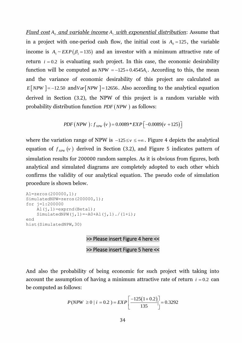
Fixed cost 0 A and variable income 1 A with exponential distribution: Assume that

in a project with one-period cash flow, the initial cost is 0 125A , the variable

income is 1 1~ 135A EXP and an investor with a minimum attractive rate of

return 0.2i is evaluating such project. In this case, the economic desirability

function will be computed as 1 125 0.4545NPW A . According to this, the mean

and the variance of economic desirability of this project are calculated as

12.50E NPW and 12656Var NPW . Also according to the analytical equation

derived in Section (3.2), the NPW of this project is a random variable with

probability distribution function PDF NPW as follows:

: 0.0089* 0.0089 125NPWPDF NPW f v EXP v

where the variation range of NPW is 125 v . Figure 4 depicts the analytical

equation of NPWf v derived in Section (3.2), and Figure 5 indicates pattern of

simulation results for 200000 random samples. As it is obvious from figures, both

analytical and simulated diagrams are completely adopted to each other which

confirms the validity of our analytical equation. The pseudo code of simulation

procedure is shown below.

A1=zeros(200000,1); SimulatedNPW=zeros(200000,1); for j=1:200000 A1(j,1)=exprnd(Beta1); SimulatedNPW(j,1)=-A0+A1(j,1)./(1+i); end hist(SimulatedNPW,30)



And also the probability of being economic for such project with taking into

account the assumption of having a minimum attractive rate of return 0.2i can

be computed as follows:

125 1 0.2

( 0 | 0.2 ) 0.3292135

P NPW i EXP

35

As it is obvious from Figures 4 and 5, the economic desirability of this project

NPW is less than zero in some cases 125, 0 , and for this reason, the probability

of being economic for this project is computed as 32.92%.

Fixed cost 0 A and variable income 1 A with uniform distribution: In this case, we

take into account a project with an initial cost 0 100A , a variable income

1 1 1~ 125, 155A Uniform and an investor with minimum attractive rate of

return 0.35i . In this case, the function of economic desirability will be as

1 100 0.7407NPW A . Therefore, the mean and the variance of economic

desirability of this project are calculated as 3.7037E NPW and

41.1523Var NPW . Also according to the analytical equation derived in Section

(3.3), the NPW of this project has a uniform distribution with probability

distribution function PDF NPW as follows:

1 10 0 ~ 7.4074, 14.8148

1 1NPW Uniform A A

i i

: 0.0450, 7.4074 14.8148NPWPDF NPW f v v

To validate this analytical equation, the simulation approach is utilized. Figures 6

and 7 confirm the adoption of analytical equation of NPWf v and the simulated

results for 200000 samples. The pseudo code for simulation procedure is shown as

follows.

A1=zeros(200000,1); SimulatedNPW=zeros(200000,1); for j=1:200000 A1(j,1)=random('unif',Alfa1,Beta1); SimulatedNPW(j,1)=-A0+A1(j,1)./(1+i); end hist(SimulatedNPW,10)



Moreover the probability of being economic for such project is gained as:

36

1 0

1 1

1( 0 | ) 0.6667

A iP NPW i

In this project, if 0.6i , since 1 0 1A i , therefore according to lemma 1, it is

certainly uneconomic and the probability of being economic equals to 0. Also if

0.2i , since 1 0 1A i , therefore according to lemma 2, this project is certainly

uneconomic and the probability of being economic equals to 1.

5.2. Numerical Examples for Two-Period Cash Flows

Fixed cost 0A , fixed income 1 A and variable income 2 A with normal distribution:

Assume that in a two-period project, the cash flow is as

2

0 1 2 2 2160, 130, ~ 100, 20A A A Normal and the minimum attractive rate of

return equals to 0.25i . In this project, the function of economic desirability NPW

derived as follows:

1 20 22

56 0.64 1 1

A ANPW A A

i i

8, 8.1920E NPW Var NPW

and, according to the results derived in Section (4.1), it can be concluded that:

~ 8, 8.1920NPW Normal

Similar to one-period cases, the comparison between derived analytical equation

and simulation results was carried out, and the results confirm the existence of

this equation completely. For simplicity and with the aim of preventing the

repetitive materials, we discard the simulation procedure hereafter. Also the

probability of being economic for this project with having minimum attractive rate

of return 0.25i is obtained as follows:

( 0 | 0.25 )P NPW i

2

0.5

160 1 0.25 130 1 0.25 1001 0.9974

20

37

Fixed cost 0 A , variable income 1 A with normal distribution and fixed income 2 A :

Assume, in the previous example, the cash flow would be as

2

0 1 1 1 2 160, 130, 20 , ~100A A Normal A and the minimum attractive rate of

return would be 0.25i . In this case, the function of economic desirability NPW

can be achieved as follows:

1 20 12

96 0.8 1 1

A ANPW A A

i i

8, 12.80E NPW Var NPW

So, according to the analytical results derived in Section (4.2), it can be concluded

that:

~ 8,1 2.80NPW Normal

Similar to the previous cases, the simulation results confirm the existence of this

equation completely. Also the probability of being economic for this project with

having minimum attractive rate of return 0.25i , is attained as follows:

( 0 | 0.25 )P NPW i

0.5

160 1 0.25 130 100 / 1 0.25 1 0.9873

20


distribution: Consider a two-period project with cash flow as

0 1 2 2160, 130, ~ 100A A A EXP and a minimum attractive rate of return as

0.25i . In this case, the function of economic desirability would be as

2NPW 56 0.64 A with 8E NPW and Var NPW 4096 . So according to the

analysis performed in Section (4.3), it can be concluded that:

1.5625 160 162.5

: 0.0156* ,100

NPW

vPDF NPW f v EXP

where the variation range of NPW is 56 v . Similar to the one-period cases,

the simulation results confirm the existence of this equation. Furthermore, the


of return 0.25i can be gained as:

38

2130 1 0.25 160 1

( 0 | 0.25 ) 0.4169100

iP NPW i EXP

But if the initial cost would be 0 A 100 instead of 0 A 160 , according to lemma 3,

since we have 1

0

1A

iA

, so this project is certainly economic in this case and the

probability of being economic will be 1.

Fixed cost 0 A , variable income 1 A with exponential distribution and fixed income

2 A : Assume that the cash flow of a two-period project is

0 1 1 2160, ~ 130 , 100A A EXP A and the minimum attractive rate of return is

0.25i . In this case, the function of economic desirability would be as

196 0.8 NPW A with 8E NPW and 10816Var NPW . So according to the

analysis performed in Section (4.4), it can be concluded that:

1.25 160 80

: 0.0096* ,100

NPW

vPDF NPW f v EXP

where variation range of the NPW would be 96 v . Similar to the previous

cases, simulation analysis was carried out and the results confirm the existence of

this equation. Additionally, the probability of being economic with having

minimum attractive rate of return 0.25i can be calculated for this project as

follows:

100 / 1 0.25 160 1 0.25

( 0 | 0.25 ) 0.3973130

P NPW i EXP

However, according to what has been proved in lemma 4, if the initial cost would

be 0 60A instead of 0 160A , we have 22

0

1A

iA

, so the project is certainly

economic and the probability of being economic is 1.

Fixed cost 0 A , fixed income 1 A and variable income 2 A with uniform distribution:

Consider a two-period project with cash flow as 0 1 160, 130, A A

2 2 2~ 80, 120A Uniform and the minimum attractive rate of return as 0.25i .

39

In this case, the economic desirability function would be as 2 56 0.64 NPW A

with 8E NPW and 54.6133Var NPW . According to the analyses performed in

Section (4.5), it can be concluded that:

2 1 2 10 02 2

~ 4.80, 20.801 11 1

A ANPW Uniform A A

i ii i

: 0.0391, 4.8 10.80NPWPDF NPW f v v

Similar to the one-period cases, the simulation analysis was carried out and the

results confirm the existence of such function completely. In addition, the


of return 0.25i is calculated as:

2120 130 1 0.25 160 1 0.25

( 0 | ) 0.8125120 80

P NPW i

But according to what has been presented in lemma 5, if the upper bound of the

income 2 A would be 2 87 , then we have 2

2 0 11 1A i A i , and the project

is certainly uneconomic with probability of being economic as 0 . In the other

hand, if the lower bound of income 2 A would be 2 90 , in this case we have

2

2 0 1 1 1A i A i and then according to lemma 6, project is certainly

economic with the probability of being economic as 1.

Fixed cost 0 A , variable income 1 A with uniform distribution and fixed income 2 A :

Consider the cash flow of a two-period project would be as

0 1 1 1 2160, ~ 110, 150 , 100A A Uniform A and the minimum attractive rate of

return is 0.25i . In this case, the function of economic desirability would be

196 0.8 NPW A with 8E NPW and 85.3333Var NPW . In this case, according

to the results derived in Section (4.6), it can be concluded that:

2 1 2 10 02 2

~ 8, 241 11 1

A ANPW Uniform A A

i ii i

: 0.0313, 8 24NPWPDF NPW f v v

40

Similar to one-period cases, the simulation results confirm the existence of this

function completely. In addition, the probability of being economic for this project

with minimum attractive rate of return 0.25i is obtained as:

100 / 1 0.25 150 160 1 0.25

( 0 | ) 0.75150 110

P NPW i

However, according to what has been proved in lemma 7, if the upper bound of

income 2 A would be 1 115 , then we have 1 0 2 1 / 1A i A i , and the project

is certainly uneconomic. In the other hand, if the lower bound of income 2 A would

be 3 130 , we have 1 0 21 / 1A i A i and, according to lemma 8, the

project is certainly economic and the probability of being economic would be 1.

5.3. Numerical Examples for Multiple-Period Cash Flows

Variable income with normal distribution: Consider an investment project

with five periods, where the cash flow is as

2

0 1 2 3 3 3400, 150, 200, ~ 100, 10A A A A Normal , 4 50A and 5 150A . In

addition, assume that the minimum attractive rate of return equals to 0.25i

. In this project, the function of economic desirability NPW derived as

follows:

5

0 3

1

82.4 0.51 1

k

k

k

ANPW A A

i

31.16, 2.62E NPW Var NPW

and, according to the results derived in Section (5.1), it can be concluded

that:

~ 31.16, 2.62NPW Normal

Similar to one and two period cases, the comparison between derived NPW

equation and simulation results was done, and the results confirm this NPW

equation completely. Also the probability of being economic for this project

41

for an investor with minimum attractive rate of return 0.25i is obtained as

follows:

( 0 | 0.25 )P NPW i

3

1 3 2 3 4 3 5 3

150 200 50 150400 1 0.25 100

1 0.25 1 0.25 1 0.25 1 0.251 0.00

10

That means this project has no chance to be economic.

Variable income with exponential distribution: Assume, in the previous

example, the cash flow at third period is 3 3 ~ 350A EXP and all other

parameters are unchanged. In this case, the mean and variance of economic

desirability NPW are achieved as follows:

96.83, 32112.64E NPW Var NPW

So, according to the analytical results derived in Section (5.2), it can be

concluded that:

3

1 3 2 3 4 3 5 33

150 200 50 150400 1 0.25

1 0.25 1 0.25 1 0.25 1 0.251 0.25:

350 350NPW

v

PDF NPW f v EXP

Similar to the previous cases, the simulation results confirm the existence of

this equation completely. Also the probability of being economic for this

project is attained as follows:

( 0 | 0.25 )P NPW i

42

3

1 3 2 3 4 3 5 3

150 200 50 150400 1 0.25

1 0.25 1 0.25 1 0.25 1 0.250.6315

350EXP

Since the condition

0

1 | 1

n

k

k

k k l

AA

i

(317.63 400) is true for this example, we

can conclude that the probability of being economic for this project is 0.6315 .

Variable income with uniform distribution: Consider previous example, in

which the cash flow at third period is 3 3 3 ~ 500, 600A Uniform and all

other parameters are unchanged. In this case, the mean and variance of

economic desirability NPW are achieved as follows:

199.23, 218.45E NPW Var NPW

So, according to the analytical results derived in Section (5.3), the PDF of

NPW can be concluded that:

31 0.25

: 0.0195, 1 73.63 224.83600 500

NPWPDF NPW f v v

As can be seen, both upper and lower bounds of NPW are greater than zero

and then ( 0 | 0.25 )P NPW i is 1. That means this project is certainly

economic.

6.‌ Conclusions

This paper utilized the probability theory tools like moment generating function

(MGF) and transformation method, to derive the analytical and closed-form

function for probability distribution function (PDF) of the net present worth

(NPW) in investment projects. The random cash flows follow normal, uniform and

exponential distributions in our analysis. This analysis was performed for three

classes of investment projects: (i) one-period cash flows including three different

cases (fixed cost 0 A and variable income 1A with normal, exponential and uniform

distributions), (ii) two-period cash flows including six different cases (fixed cost 0 A

43

, fixed income 1 A and variable income 2 A with normal, exponential and uniform

distributions, and fixed cost 0 A , variable income 1 A with normal, exponential and

uniform distributions and fixed income 2 A ) and (iii) multiple period cash flows

with normal, exponential and uniform distributions of incomes. The probability

distribution functions of NPW are derived for each cases separately. To validate

the analytical PDFs derived, numerical examples are presented and a set of

comprehensive simulation analysis was conducted. The comparisons performed

between simulation results and analytical functions. The simulated results

demonstrated that both analytical and simulated results of derived PDFs are

completely adopted to each other, which confirms the validity of our analytical

equations. The importance of such PDF functions is that the investor can simply

calculate the probability of being economic for investment projects and get more

reliable decisions. In deterministic economic evaluation problems, the investor has

his/her own minimum attractive rate of return (MARR) which is used in project

evaluations. In our stochastic problems, we calculate the probability of being

economic for an uncertain cash flow. When this parameter is calculated, the

investor can compare this parameter with his/her minimum probability of being

economic. If the minimum probability of being economic is satisfied, the project is

selected as economic, and otherwise, it is rejected. In other words, this paper

presented a decision-making tool for evaluation of investment projects with

uncertain cash flows.

An interesting direction for future study is to consider other performance criteria

like NFW, NEUA, or even payback period, with other probability distributions like

Weibull or Gamma.

References

1. Cleland, D., and Ireland, L. "Project management: Strategic design and implementation". New york: McGraw Hill (2002).

2. Carlsson, C., Fuller, R., Heikkila, M., and Majlender, P. "A fuzzy approach to R&D project portfolio selection". International Journal of Approximate Reasoning, 44(2), pp. 93–105 (2007).

3. Chen, T., Zhang, J., and Lai, K. "An integrated real options evaluating model for information technology projects under multiple risks". International Journal of Project Management, 27(8), pp. 776-786 (2009).

44

4. Armaneri, Ö., Özdagoglu, G., and Yalçinkaya, Ö. "An integrated decision support approach for project investors in risky and uncertain environments". Journal of Computational and Applied Mathematics, 234(8), pp. 2530-2542 (2010).

5. Zhang, W. G., Me, Q., Lu, Q., and Xiao, W. L. "Evaluating methods of investment project and optimizing models of portfolio selection in fuzzy uncertainty". Computers and Industrial Engineering, 61(3), pp. 721-728 (2011).

6. Hanafizadeh, P., and Latif, V. "Robust net present value", Mathematical and Computer Modelling, 54(1-2), pp. 233-242 (2011).

7. Wang, J., and Hwang, W. L. "A fuzzy set approach for R&D portfolio selection using a real options valuation model". Omega, 35(3), pp. 247-257 (2007).

8. Zuojun, P., Yuhong, C., and Lei, S. "Applied research on improved fuzzy chance-constrained model in engineering project comparison and selection". Procedia Engineering, 12(1), pp. 184-190 (2011).

9. Ebrahimnejad, S., Mousavi, S., Tavakkoli-Moghaddam, R., Hashemi, H., and Vahdani, B. "A novel two-phase group decision making approach for construction project selection in a fuzzy environment". Applied Mathematical Modelling, 36(9), pp. 4197-4217 (2011).

10. Chiang, T. A., and Che, Z. "A fuzzy robust evaluation model for selecting and ranking NPD projects using Bayesian belief network and weight-restricted DEA". Expert Systems with Applications, 37(11), pp. 7408-7418 (2010).

11. Shakhsi-Niaei, M., Torabi, S., and Iranmanesh, S. "A comprehensive framework for project selection problem under uncertainty and real-world constraints". Computers & Industrial Engineering, 61(1), pp. 226-237 (2011).

12. Huang, X. "Optimal project selection with random fuzzy parameters". International Journal Production Economics, 106(2), pp. 513-522 (2007).

13. Naimi Sadigh, A. Mokhtari, H., Iranpoor, M., and Ghomi, S. M. T. "Cardinality constrained portfolio optimization using a hybrid approach based on particle swarm optimization and Hopfield neural network". Advanced Science Letters, 17(1), pp. 11-20 (2012).

14. Salmasnia, A., Mokhtari, H., and Abadi, I. N. K. "A robust scheduling of projects with time, cost, and quality considerations". The International Journal of Advanced Manufacturing Technology, 60(5-8), pp. 631-642 (2012).

15. Liu, M., and Wu, F. F. "Portfolio optimization in electricity markets". Electric Power systems research, 77(8), pp. 1000-1009 (2007).

16. Afshar-Nadjafi, B., Parsanejad, A., Hajipour, V., and Nobari, A. "Solution procedure for generalized resource investment problem with discounted cash flows and progress payment". Scientia Iranica, 21(6), pp. 2436-2447 (2014).

45

17. Rębiasz, B., and Macioł, A. "Comparison of Classical Multi-Criteria Decision Making Methods with Fuzzy Rule-Based Methods on the Example of Investment Projects Evaluation". In Intelligent Decision Technologies , pp. 549-561). Springer, Cham (2015).

18. Dai, C. Y., Wang, Y. X., Li, D., and Zhou, Y. L. "Renewable Energy Investment Project Evaluation Model Based on Improved Real Option. In Low-carbon City and New-type Urbanization" (pp. 43-53). Springer, Berlin, Heidelberg (2015).

19. Kilic, M., and Kaya, İ. "Investment project evaluation by a decision making methodology based on type-2 fuzzy sets". Applied Soft Computing, 27(1), pp. 399-410 (2015).

20. Kirkwood, L., Shehab, E., Baguley, P., and Starr, A. "Uncertainty of Net Present Value calculations and the impact on applying integrated maintenance approaches to the UK rail industry". Procedia CIRP, 38(1), pp. 245-249 (2015).

21. Tabrizi, B. H., Torabi, S. A., and Ghaderi, S. F. "A novel project portfolio selection framework: An application of fuzzy DEMATEL and multi-choice goal programming". Scientia Iranica, 23(6), pp. 2945-2958 (2016).

22. Fathallahi, F., and Naja, A. A. "A hybrid genetic algorithm to maximize net present value of project cash flows in resource-constrained project scheduling problem with fuzzy parameters". Scientia Iranica, 23(4), pp. 1893-1903 (2016).

23. Dutta, G., and Ashtekar, M. "A system dynamics simulation model of a blast furnace for project evaluation". International Journal of Business and Systems Research, 11(3), pp. 325-343 (2017).

24. Etemadi, S., Koosha, H., and Salari, M. "A goal programming capital budgeting model under uncertainty in Construction industry". Scientia Iranica, 25(2), pp. 841-851 (2018).

25. Mohagheghi, V., Mousavi, S. M., Vahdani, B., and Shahriari, M. R. "R&D project evaluation and project portfolio selection by a new interval type-2 fuzzy optimization approach". Neural Computing and Applications, 28(12), pp. 3869-3888 (2017).

26. Awasthi, A., and Omrani, H. "A scenario simulation approach for sustainable mobility project evaluation based on fuzzy cognitive maps". International Journal of Modelling and Simulation, pp. 1-11 (2018).

27. Montgomery, D. C., and Runger, G. C. "Applied statistics and probability for engineers". New York: John Wiley And Sons (2010).

28. Ross, S. "A First Course in Probability", 7th edition. Upper Saddle River, NJ: Pearson (2005).

46

Hadi Mokhtari is currently an Assistant Professor of Industrial Engineering in

University of Kashan, Iran. His current research interests include the

applications of operations research and artificial intelligence techniques to the

areas of project scheduling, production scheduling, manufacturing supply

chains, and engineering economic problems. He also published several papers

in international journals such as Computers and Operations Research,

International Journal of Production Research, Applied Soft Computing,

Neurocomputing, International Journal of Advanced Manufacturing Technology,

IEEE Transactions on Engineering Management, and Expert Systems with

Applications.

Saba Kiani is currently a B.Sc. student of Industrial Engineering in University

of Kashan, Iran. Her current research interests include the applications of

operations research and applied statistics to the areas of engineering

economics problems.

Seyed Saman Tahmasebpoor is currently a B.Sc. student of Industrial

Engineering in University of Kashan, Iran. His current research interests

include the applications of operations research and applied statistics to the

engineering economics problems.

Captions:

Figure 1: A multiple-period cash flow diagram

Figure 2: The NPW distribution function according to the analytical equation derived for project with fixed cost 0 A and variable income 1 A with normal distribution

Figure 3: The NPW distribution histogram according to the simulation results for project with fixed cost 0A and variable income 1 A with normal distribution

Figure 4: The NPW distribution function according to the analytical equation derived for project with fixed cost 0 A and variable income 1 A with exponential distribution

Figure 5: The NPW distribution histogram according to the simulation results for project with fixed cost 0 A and variable income 1 A with exponential distribution

Figure 6: The NPW distribution function according to the analytical equation derived for project with fixed cost 0 A and variable income 1 A with exponential distribution

Figure 7: The NPW distribution histogram according to the simulation results for project

with fixed cost 0 A and variable income 1 A with exponential distribution

47

Tables: −

Figure 1: A multiple-period cash flow diagram

Figure (3): The NPW distribution histogram according to the simulation results for project with

fixed cost 0A and variable income 1 A with normal

distribution

Figure (2): The NPW distribution function according to the analytical equation derived

for project with fixed cost 0 A and variable

income 1 A with normal distribution

4 6 8 10 12 14 16 180

1

2

3

4x 10

4

Sim

ula

ted P

DF

4 6 8 10 12 14 16 180

0.05

0.1

0.15

0.2

0.25

0.3

Ana

lytical P

DF

-175 -75 25 125 225 325 425 525 625 725 8000

1

2

3

4

5

6x 10

4

Sim

ula

ted P

DF

-175 -75 25 125 225 325 425 525 625 725 8000

0.002

0.004

0.006

0.008

0.01

Analy

tical P

DF

𝐴0

𝐴1

0

1

𝐴2

2

𝐴𝑛

𝑛

48

Figure (5): The NPW distribution histogram according to the simulation results for project

with fixed cost 0 A and variable income 1 A with

exponential distribution

Figure (4): The NPW distribution function according to the analytical equation derived for

project with fixed cost 0 A and variable income 1 A

with exponential distribution

Figure (7): The NPW distribution histogram according to the simulation results for project

with fixed cost 0 A and variable income 1 A with

exponential distribution

Figure (6): The NPW distribution function according to the analytical equation derived for

project with fixed cost 0 A and variable income

1 A with exponential distribution

Tables: −

-10 -8 -6 -4 -2 0 2 4 6 8 10 12 14 16170

0.5

1

1.5

2

2.5x 10

4

Sim

ula

ted P

DF

-10 -8 -6 -4 -2 0 2 4 6 8 10 12 14 16170

0.01

0.02

0.03

0.04

0.05

0.06

Analy

tical P

DF

Economic Evaluation of Investment Projects Under...

Documents

Transcript of Economic Evaluation of Investment Projects Under...