ECONOMIC EFFICIENCY OF AIR NAVIGATION SERVICE PROVIDERS: AN

ASSESSMENT IN EUROPE

by

Rui Neiva

A Dissertation

Submitted to the

Graduate Faculty

of

George Mason University

in Partial Fulfillment of

The Requirements for the Degree

of

Doctor of Philosophy

Public Policy

Committee:

Kenneth Button, Chair

John Earle

Lance Sherry

John Strong, External Reader

James P. Pfiffner, Program Director

Mark J. Rozell, Dean

Date: Spring Semester 2014

George Mason University

Fairfax, VA

Economic Efficiency of Air Navigation Service Providers: An Assessment in Europe

A Dissertation submitted in partial fulfillment of the requirements for the degree of

Doctor of Philosophy at George Mason University

by

Rui Neiva

Bachelor in Engineering Sciences

University of Porto, 2007

Master in Civil Engineering

University of Porto, 2009

Director: Kenneth Button, University Professor

School of Public Policy

Spring Semester 2014

George Mason University

Fairfax, VA

ii

This work is licensed under a creative commons

attribution-noderivs 3.0 unported license.

iii

DEDICATION

To my Parents.

iv

ACKNOWLEDGEMENTS

I would like to thank my dissertation committee chair, Professor Ken Button, for all the

support and guidance throughout the entire doctoral program. I would also like to thank

the other two members of the committee, Professors John Earle and Lance Sherry, for

their help during the field and dissertation stages of the program, and to Professor John

Strong for accepting to be my external reader.

I am also thankful to all my friends on both sides of the Atlantic for their continuous

friendship throughout the entire program. In the United States, Rebecca Mao, Robin

Skulrak, and Tameka Porter; special thanks to Carla Cerqueira for making the last weeks

of writing much more enjoyable. Back in Portugal, André Domingues, Maria João

Saleiro, Manuela Carvalho, Marina Carneiro, and Tiago Tarrataca.

Finally, and most of all, I am grateful to my family, especially my Parents and my sister

Filipa for their support.

This dissertation and my doctoral studies had the financial support of the Fundação para a

Ciência e Tecnologia, with the scholarship SFRH/BD/64730/2009, funded under the

POPH and QREN Portugal programs.

v

TABLE OF CONTENTS

Page

List of Tables ................................................................................................................... viii

List of Figures ..................................................................................................................... x

List of Equations ................................................................................................................ xi

List of Abbreviations and Symbols................................................................................... xii

Abstract ............................................................................................................................ xiv

Chapter 1 – Introduction ..................................................................................................... 1

1.1. Motivation ............................................................................................................ 1

1.1.1. Relevance of Research for Public Policy ...................................................... 1

1.1.2. Relevance for the Literature.......................................................................... 2

1.1.3. Research Questions ....................................................................................... 3

1.2. Overview of the Dissertation ............................................................................... 4

Chapter 2 – Regulation: Theory .......................................................................................... 5

2.1. The Rationale for Economic Regulation .............................................................. 5

2.2. The Changes in Regulatory Paradigm .................................................................. 6

2.2.1. Alfred E. Kahn .............................................................................................. 6

2.2.2. The Chicago School and the Capture Theory ............................................. 14

Chapter 3 – Regulation: Practice ...................................................................................... 19

3.1. Different Forms of Regulation ........................................................................... 19

3.1.1. Rate-of-Return Regulation .......................................................................... 19

3.1.2. Price-Capping ............................................................................................. 22

3.1.3. Auctioning Monopolies .............................................................................. 23

3.1.4. Ramsey Pricing ........................................................................................... 26

3.1.5. Vogelsang-Finsinger Mechanism ............................................................... 27

3.2. Regulatory Changes in the Transportation Sector.............................................. 29

3.3. Regulatory Changes in the Aviation Industry .................................................... 33

3.3.1. Airlines ........................................................................................................ 33

vi

3.3.2. Airports ....................................................................................................... 37

3.4. Benchmarking and Benchmarking Studies in the Airport Industry ................... 41

Chapter 4 – Air Navigation Services ................................................................................ 48

4.1. Historical and Technical Notes .......................................................................... 48

4.2. Commercialization and Privatization ................................................................. 52

4.3. Current Developments........................................................................................ 56

4.3.1. Europe – Single European Sky ................................................................... 56

4.3.2. United States – NextGen ............................................................................. 68

Chapter 5 – Benchmarking Air Navigation Services: Literature Review ......................... 71

Chapter 6 – Methodology ................................................................................................. 89

6.1. Qualitative Assessments ..................................................................................... 89

6.1.1. SWOT Analysis .......................................................................................... 89

6.1.2. Case Studies ................................................................................................ 93

6.2. Quantitative Assessments ................................................................................... 93

6.2.1. Data Envelopment Analysis ........................................................................ 94

6.2.2. Stochastic Frontier Analysis ..................................................................... 101

6.2.3. Identification Issues .................................................................................. 103

6.2.4. Discussion of Quantitative Methodologies ............................................... 106

6.2.5. Data Sources ............................................................................................. 108

Chapter 7 – Qualitative Assessments .............................................................................. 111

7.1. SWOT Analysis................................................................................................ 111

7.2. Case Studies of Selected Markets .................................................................... 120

7.2.1. Canada....................................................................................................... 120

7.2.2. New Zealand ............................................................................................. 122

7.2.3. United Kingdom........................................................................................ 125

7.2.4. United States ............................................................................................. 134

Chapter 8 – Data Envelopment Analysis ........................................................................ 138

8.1. Model Specification ......................................................................................... 138

8.2. Results .............................................................................................................. 147

8.3. Spatial Autocorrelation Issues .......................................................................... 158

8.4. Total Factor Productivity ................................................................................. 163

8.5. An Analysis of the Functional Airspace Blocks .............................................. 165

vii

8.6. Difference-in-Differences ................................................................................ 174

8.7. Discussion ........................................................................................................ 176

Chapter 9 – Stochastic Frontier Analysis........................................................................ 177

9.1. Model Specification ......................................................................................... 177

9.2. Results .............................................................................................................. 181

9.3. Discussion ........................................................................................................ 186

Chapter 10 – Conclusions ............................................................................................... 188

10.1. Research Findings......................................................................................... 188

10.2. Policy Implications ....................................................................................... 191

10.3. Research Limitations .................................................................................... 194

10.4. Other Considerations .................................................................................... 197

10.4.1. Challenges in Commercialization ......................................................... 197

10.4.2. Capacity and Innovation........................................................................ 199

Appendix I – ANSP Features .......................................................................................... 201

Appendix II – ANSP DEA Analysis: Tables .................................................................. 202

Appendix III – ANSP DEA Analysis: Figures ............................................................... 218

Appendix IV – ANSP DEA Analysis: Regressions ........................................................ 235

Appendix V – FAB DEA Analysis: Tables .................................................................... 240

Appendix VI – FAB DEA Analysis: Figures ................................................................ 245

Appendix VII – FAB DEA ANALYSIS: Regressions .................................................. 249

Appendix VIII – ANSP SFA Analysis: Tables............................................................... 251

Appendix IX – ANSP SFA Analysis: Figures ................................................................ 267

Appendix X – ANSP SFA Analysis: Regressions .......................................................... 269

References ....................................................................................................................... 272

viii

LIST OF TABLES

Table Page

Table 1 Possible models of private sector involvement in infrastructure provision. ........ 38 Table 2 The influences promoting privatization ............................................................... 40

Table 3 Basic features of selected air navigation service providers ................................. 56 Table 4 US and European Air Navigation Systems (2012) .............................................. 57

Table 5 Basic statistics of the FABs (2011)...................................................................... 66 Table 6 Financial and economic KPIs for the FABs (2011) ............................................. 66 Table 7 Selected NextGen projects with cost and schedules performance ....................... 70 Table 8 Financial and economic KPIs for the individual ANSPs (2011) ......................... 74

Table 9 Financial and economic KPIs for the FABs (2011) ............................................. 74 Table 10 Performance ratios for the different components of the financial KPI and

employment costs for the individual ANSPs (2011) ........................................................ 75 Table 11 IFR flight-hours per ATCo in operations (worldwide data) .............................. 82 Table 12 Cost per IFR flight-hour (worldwide data) ........................................................ 83

Table 13 Employment costs for ATCo in operations per IFR flight-hour (worldwide data)

........................................................................................................................................... 84 Table 14 The basis of SWOT analysis. ............................................................................. 91 Table 15 SWOT analysis of ANSs provision. ................................................................ 113

Table 16 Financial information on Airways New Zealand. ............................................ 125 Table 17 Some statistics for UK’s ANSP ....................................................................... 131

Table 18 Basic statistics for the variables included in the DEA analysis. ...................... 145 Table 19 Correlation matrix for DEA regression ........................................................... 146

Table 20 DEA bootstrap regression results .................................................................... 155 Table 21 Moran’s I spatial autocorrelation measures ..................................................... 163 Table 22 Basic statistics for the variables included in the FAB DEA analysis. ............. 167 Table 23 Correlation matrix for FAB DEA regression ................................................... 171 Table 24 FAB DEA regression results............................................................................ 172

Table 25 Differences-in-differences estimate ................................................................. 175 Table 26 Basic statistics for the variables included in the SFA analysis. ....................... 181

Table 27 SFA main regression results for Cobb-Douglas specification ......................... 182 Table 28 SFA main regression results for translog specification ................................... 182 Table 29 SFA specifications likelihood ratio tests ......................................................... 183 Table 30 DEA vs. SFA efficiencies comparison ............................................................ 184 Table 31 DEA vs. SFA explanatory variables comparison ............................................ 186

Table 32 Air navigation service providers ownership features ...................................... 201 Table 33 DEA efficiency results ..................................................................................... 202

ix

Table 34 DEA allocative efficiency results .................................................................... 205 Table 35 DEA inputs and outputs slacks ........................................................................ 208 Table 36 DEA total factor productivity Malmquist indexes ........................................... 215 Table 37 DEA regression with temporal dummy variables ............................................ 235

Table 38 DEA regression with geographical dummy variables ..................................... 236 Table 39 DEA regression results with COMPLEX variable .......................................... 238 Table 40 DEA regression results with DENS and STRUCT variables .......................... 239 Table 41 DEA efficiency results – FAB analysis ........................................................... 240 Table 42 DEA allocative efficiency results – FAB analysis ........................................... 242

Table 43 DEA inputs and outputs slacks – FAB analysis .............................................. 243 Table 44 FAB regression results with temporal dummy variables ................................. 249

Table 45 FAB regression results with geographical dummy variables .......................... 250 Table 46 SFA efficiencies for Cobb-Douglas specifications .......................................... 251 Table 47 SFA efficiencies for translog specifications .................................................... 259 Table 48 SFA mean efficiencies by year for Cobb-Douglas specification ..................... 266

Table 49 SFA mean efficiencies by year for translog specification ............................... 266 Table 50 SFA regression results for Cobb-Douglas specification .................................. 269

Table 51 SFA regression results for translog specification ............................................ 270

x

LIST OF FIGURES

Figure Page

Figure 1 Different levels of government involvement in airports. ................................... 38 Figure 2 The different components of air navigation services ......................................... 51

Figure 3 Flight information regions in European airspace ............................................... 58 Figure 4 Details about the costs of fragmentation in the Europe ANSs system ............... 59

Figure 5 The functional airspace blocks. .......................................................................... 65 Figure 6 CCR vs. BCC models comparison ..................................................................... 98 Figure 7 Differences-in-differences ................................................................................ 104 Figure 8 DEA efficiency results for UK’s NATS ........................................................... 133

Figure 9 DEA efficiency results for each year ................................................................ 153 Figure 10 DEA relative efficiencies for 2011 ................................................................. 162

Figure 11 DEA total factor productivity Malmquist indexes – yearly averages ............ 164 Figure 12 DEA efficiency results for the FAB analysis ................................................. 168 Figure 13 DEA vs. SFA (translog) efficiencies comparison .......................................... 185

Figure 14 DEA efficiency results for each year .............................................................. 222

Figure 15 DEA results for each ANSP ........................................................................... 228 Figure 16 DEA total factor productivity Malmquist indexes for each ANSP ................ 234 Figure 17 DEA FAB results for each year ...................................................................... 246

Figure 18 DEA results for each FAB .............................................................................. 248 Figure 19 SFA mean efficiencies by year for Cobb-Douglas specification ................... 267

Figure 20 SFA mean efficiencies by year for translog specification .............................. 268

xi

LIST OF EQUATIONS

Equation Page

Equation 1 ......................................................................................................................... 20 Equation 2 ......................................................................................................................... 20

Equation 3 ......................................................................................................................... 96 Equation 4 ......................................................................................................................... 97

Equation 5 ......................................................................................................................... 99 Equation 6 ....................................................................................................................... 100 Equation 7 ....................................................................................................................... 101 Equation 8 ....................................................................................................................... 102

Equation 9 ....................................................................................................................... 104 Equation 10 ..................................................................................................................... 129

Equation 11 ..................................................................................................................... 130 Equation 12 ..................................................................................................................... 160 Equation 13 ..................................................................................................................... 160

Equation 14 ..................................................................................................................... 177

Equation 15 ..................................................................................................................... 179 Equation 16 ..................................................................................................................... 179

xii

LIST OF ABBREVIATIONS AND SYMBOLS

Advance Automation System ........................................................................................AAS

Air Navigation Service Provider ................................................................................. ANSP

Air Navigation Services ............................................................................................... ANSs

Air Traffic Control .........................................................................................................ATC

Air Traffic Controller ...................................................................................................ATCo

Air Traffic Flow Management ................................................................................... ATFM

Air Traffic Management ............................................................................................... ATM

Air Traffic Organization ............................................................................................... ATO

Area Control Centers .................................................................................................... ACC

ATM Cost-Effectiveness ...............................................................................................ACE

Automatic Dependent Surveillance – Broadcast .......................................................ADS-B

Banker, Charnes, and Cooper (DEA model) .................................................................BCC

Charnes, Cooper, and Rhodes (DEA model) .................................................................CCR

Civil Aeronautics Board ............................................................................................... CAB

Civil Air Navigation Services Organisation ............................................................ CANSO

Communications, Navigation and Surveillance ............................................................. CNS

Consumer Price Index ..................................................................................................... CPI

Corporación Centroamericana de Servicios de Navegación Aérea .................... COCESNA

Cost-Benefit Analysis ................................................................................................... CBA

Data Envelopment Analysis .......................................................................................... DEA

Decision Making Unit .................................................................................................. DMU

Differences-in-Differences .......................................................................................... D-i-D

Dollar ...................................................................................................................................$

Euro ......................................................................................................................................€

European Aviation Safety Agency.............................................................................. EASA

European Union ............................................................................................................... EU

Federal Aviation Administration ...................................................................................FAA

Flight Information Region ............................................................................................ FIR

Functional Airspace Block ............................................................................................. FAB

Instrument Flight Rules ................................................................................................. IFR

Interstate Commerce Commission .................................................................................. ICC

Key Performance Indicator ............................................................................................. KPI

L'Agence pour la Sécurité de la Navigation aérienne en Afrique et à Madagascar ...............

…………………………………………………………………………………...ASECNA

Maastricht Upper Area Control Centre ......................................................................MUAC

National Air Traffic Services Ltd ............................................................................... NATS

xiii

Nautical Miles ............................................................................................................... NM

Next Generation Air Transportation System .......................................................... NextGen

Performance Review Report .......................................................................................... PRR

Professional Air Traffic Controllers Organization .................................................. PATCO

Public-Private Partnership .............................................................................................. PPP

Single European Sky ATM Research ....................................................................... SESAR

Single European Sky ....................................................................................................... SES

Stochastic Frontier Analysis .......................................................................................... SFA

Strengths, Weaknesses, Opportunities, and Threats .................................................. SWOT

Total Factor Productivity ................................................................................................ TFP

United Kingdom............................................................................................................... UK

United States of America ................................................................................................. US

Upper Information Region .............................................................................................. UIR

US Air Traffic Services Corporation ........................................................................ USATS

Vogelsang-Finsing (mechanism) .................................................................................... V-F

xiv

ABSTRACT

ECONOMIC EFFICIENCY OF AIR NAVIGATION SERVICE PROVIDERS: AN

ASSESSMENT IN EUROPE

Rui Neiva, Ph.D.

George Mason University, 2014

Dissertation Director: Dr. Kenneth Button

The economic deregulation efforts that have been taking place for several decades

in many industries have been associated, in numerous benchmarking studies, with

improvements in economic efficiency.

The aviation industry is no exception. Research on airlines and airports has

demonstrated significant advantages in moving to a liberalized system of provision and

regulation. However, airports and airlines are just two components of the aviation

industry. The third component, air navigation service providers, links airports and airlines

as well as dispenses air traffic control services. In this industry, economic deregulation

has also been happening since the late 1980’s. Many national systems have now been

“commercialized” in attempts to improve their efficiency by separating them from their

respective governments, but research on the impact of those institutional and regulatory

xv

reforms has been somewhat scarce. This gap in the literature is what this dissertation

aims to address.

Using panel data from Europe, programmatic and econometric approaches will

estimate if these institutional changes have been associated with improvements in the

economic efficiency levels of this industry. Issues like the fragmentation of European

airspace and the existence of spatial autocorrelation will also be addressed.

Results indicate that non-commercialized providers are associated with higher

levels of economic efficiency. However surprising, these results might be affected by

limitations of the dataset, which only runs for 10 years; causality tests were used but they

did not help to further clarify the matter.

Estimates also show that a number of operational and physical variables also

significantly impact the efficiency results, and there are indications to suggest that the

great level of fragmentation of the European airspace is indeed impacting the overall

efficiency of the system.

Keywords: Economic Efficiency, Air Traffic Management, Air Navigation

Services, Air Navigation Service Providers, EUROCONTROL, Single European Sky,

Data Envelopment Analysis, Stochastic Frontier Analysis

1

CHAPTER 1 – INTRODUCTION

The aviation industry has three basic components, with air navigation services

(ANSs) and their providers, the air navigation service providers (ANSPs), being the link

that connects the other components, the airlines and the airports. Their aim is, above all

else, to assure the safety of operations and to promote an efficient flow of traffic.

Traditionally, ANSPs have been government owned and controlled, but this is no

longer the case in many countries as nations have moved to commercialize ANSPs. The

research presented in this dissertation will discuss the changing regulatory thinking that

lead public authorities to move away from the direct provision of ANSs, how those

changes have been operationalized, and estimate the possible effects, if any, of those

changes in terms of economic efficiency.1

1.1. Motivation

1.1.1. Relevance of Research for Public Policy This dissertation will not contribute to any discussion about how technology can

improve ANSs. This dissertation will focus on policy, institutions, and regulation. With

that in mind, it can provide insights and facilitate the discussion from a policy standpoint

in the area of regulation and ownership. In a time when governments are reassessing their

1 For the context of this dissertation, economic efficiency will simply be defined as the efficient use of

resources in a way that maximizes the production of services. The traditional technical and allocative

efficiency definitions will be considered, with the former being how efficiently a given set of inputs is

transformed into outputs, and the latter being defined as using the least costly input mix to produce a given

set of outputs.

2

role in society, the ANSs industry will not be exempt from that discussion. This

dissertation will add to that discussion by presenting and examining the merits and

drawbacks of the various solutions that exist. It will also use available empirical data to

benchmark how systems operating under different regulatory circumstances have

performed.

Comparing experiences and benchmarking can improve the discussion regarding

regulation by reducing the asymmetries of information between the different stakeholders

involved, thus contributing to a more informed discussion along with an improved

decision-making process. Although this dissertation will focus on one specific industry –

air navigation services –its relevance will not be limited to this industry. The history of

regulation has shown that findings about the effects of regulation on one industry could

be applicable to other industries. By adding to the body of knowledge about regulation

and ownership, this dissertation will contribute to those discussions.

1.1.2. Relevance for the Literature

Most of the literature regarding ANSs is about technical aspects. Such is also the

case of productivity and efficiency analysis in the industry. Since the commercialization

efforts started, there have been some publications that have focused on the institutional

aspects of those efforts, but mostly from an institutional perspective, not an

economic/econometric one. This dissertation will add to that body of literature by

performing an economic analysis of industry efficiency as well as an institutional

analysis. The main addition to the literature will be the explicit inclusion of ownership

variables in the economic efficiency assessments, which has not been done before. This

3

will provide insights into how commercialization has been associated with different

economic efficiency outcomes.

1.1.3. Research Questions The main goal of this research is to estimate if ownership structure has been

associated with different outcomes of economic efficiency of European air navigation

service providers. The following research questions and hypotheses are addressed:

1. Are “commercialized” ANSPs associated with higher levels of economic

efficiency than “public agency” ANSPs?

2. Is the impact of non-policy variables, namely operational and physical

ones, significant in terms of explaining differences in economic efficiency?

The first question addresses the fundamental issue of the relationship between

ownership structure and economic efficiency, and how it relates to the overall issue of the

rationale for privatization and corporatization: it has been hypothesized and shown that it

is expected that changing ownership from the public to the private sector or to private-

like business models will be associated with increased economic efficiency. This seems

to be due largely to the presence of pressures for the actions of management to match the

goals of the owners/shareholders and to innovate (Bös, 1991; Jasiński & Yarrow, 1996).2

The second question relates to how operational (e.g., number of flights controlled

or number of employees) and physical (e.g., size of airspace) variables are associated

with the economic efficiency outcomes. This is based on the understanding that ANSPs

operate in a particular industry, which is subject to a number of constraints resulting from

2 Oum et al. (2008) performs a survey with some contradictory findings, suggesting that in some cases

privatization did not results in increased efficiency.

4

the specificities of the air navigation systems themselves that cannot be easily changed, if

at all, by management, namely their physical characteristics (size of airspace, location of

airports, etc.), and the operational environment in which the systems operate (e.g.,

number of flights using the airspace). The hypothesis will assess the extent to which

those non-policy variables are associated with economic efficiency.

1.2. Overview of the Dissertation The dissertation begins with an overview of regulatory changes in the past few

decades and the move to deregulation3, from both a theoretical (Chapter 2) and practical

application (Chapter 3) perspective, with the latter being focused on applications in the

aviation industries.

The dissertation will then discuss air navigation services and air navigation

service providers (Chapter 4). First, a few historical and technical notes about the ANSs

will be presented (Chapter 4.1), followed by an examination of commercialization

practices in the industry (Chapter 4.2). Current developments in the industry will also be

presented (Chapter 4.3), with a focus on the United States and Europe.

The next chapter, Chapter 5, will present and discuss the proposed qualitative and

quantitative methodologies, along with the data sources.

The following three chapters present the results, with the first (Chapter 6) being

dedicated to the qualitative assessments, and the other two to the quantitative ones

(Chapter 7 and 8). Finally, Chapter 9 presents and discusses the conclusions.

3 Or liberalization as it is often called in Europe.

5

CHAPTER 2 – REGULATION: THEORY

This dissertation is part of a long tradition of the study of the effects of economic

regulation. This chapter will provide some background on the issue of regulation and

why, in some cases, it has been deemed necessary throughout history.

In addition to the general historical perspective, a more detailed examination of

the aviation industry will take place. This industry has seen major changes in the past few

decades, which have been accompanied by a plethora of studies assessing the outcomes

of those changes. The dissertation will study those regulatory changes in a particular

industry of the aviation sector: the air navigation services industry.

2.1. The Rationale for Economic Regulation Regulation has been seen as the “government’s necessary and beneficial response

to market failure” (Coppin & High, 1999, p. 8) to “induce firms […] to act in a way that

is compatible with social goals” (Train, 1991, p. xi), i.e., maximize (or at least not harm)

social welfare. For those reasons, regulation becomes needed4 when the presence of a

market along with Adam Smith’s invisible hand is not enough of a guarantee of socially

desirable outcomes and the public interest is not protected (Train, 1991).5

4 In case it is believed that one of the roles of government is to deal with market failures, as it also can be

argued that should not be a role of government. 5 This is mostly a modern definition. McCraw (1984, p. 301) expands on the purposes of regulation along

the decades: disclosure and publicity, protection and cartelization of industries, containment of monopoly

and oligopoly, promotion of safety for consumers and workers, or legitimization of the capitalist order.

6

While a simple concept in principle, the practical applications of regulation have

followed the predominant economic concepts, the political thinking that backed them up,

and the economic conditions of each period. This resulted in regulation being applied

with significant differences along the decades, from the presence of economic regulation

in a wide range of industries in the post-World War II markets, to the deregulation efforts

of the late 20th

century.

After this introduction, this section will look at the historical background and the

changes in the concept and implementation of regulation, with a focus on some of the

seminal works in the area, namely the works of Alfred E. Kahn and the economists of the

University of Chicago – the “Chicago School”. Although economic regulation has a long

history, dating at least since the 19th

century6, this chapter will focus on the period of time

since the middle of the 20th

century, as the developments made in this realm during that

period are the most relevant for the present regulatory environment and the scope of this

dissertation.

2.2. The Changes in Regulatory Paradigm

2.2.1. Alfred E. Kahn

Alfred E. Kahn was an American economist that played a pivotal role in the

development of regulatory thinking in the 1960’s and 1970’s, both in academia and in

public service as the chairman of the New York Public Service Commission and the Civil

Aeronautics Board (CAB) (McCraw, 1984).

6 Posner (1971) traces back economy regulation in the United States to 1827 in Illinois’ ferries, turnpikes,

and toll roads. For more on the history of regulation see, among others, Kolko (1963), McCraw (1984),

High (1991), Coppin & High (1999), and Glaeser & Shleife (2003).

7

To the theoretical treatment of economic regulation, Kahn’s contributions are

perhaps best represented in his two-volume seminal book “The Economics of Regulation:

Principles and Institutions” (Kahn, 1970, 1971), where issues relating to the economic

and institutional implementation of regulation were explored in great detail.

The first volume underscores the need for and implementation of economic

regulation. The volume is a presentation of the main concerns regarding the regulatory

frameworks of the time and is also a discussion of the economic principles that could be

used to improve them.

Kahn’s criticism of the regulatory procedures fell into three main categories:

quality of service, rate levels, and the rate structure.

The lack of market competition under regulation, especially for those, like public

utilities, that enjoyed a market monopoly, did not provide many incentives7 for the firms

to pay attention to quality of service. Since the regulators were concerned with rate

levels, quality of service was often seen as being the responsibility of the firm. As those

firms had no incentives to improve quality of service, it remained subpar8. On the other

hand, the regulatory framework did offer some indirect incentives in terms of quality of

service, namely because the prevailing rate-of-return regulation that was put in place

offered an incentive for overinvestments in capital9. As such, firms could invest on

improving service, knowing that the regulators would allow them to reap benefits from it.

7 The issue of incentives and how the regulatory structure of the time did not create them permeates the two

volumes of the book. 8 That was not the case in all industries. As it will be discussed later, a criticism of the airline regulation put

in place at the time was that since airlines could not compete on price, they had to compete by offering

more perks than their competitors. 9 The rate-of-return regulation and how it leads to overinvestments by firms will be discussed in Chapter

3.1.

8

Additionally, the public was critical about the failures of regulated firms in providing

adequate service, so the firms would act to avoid intervention of the regulators in

response to those criticisms.

Regarding rate level and how it should be established, the author points to several

issues. First, there is the issue of the asymmetry of information. Since companies know

much more about their own business than the regulators, there are incentives for the firms

to disclose the information that would work best for their own benefit – for example, by

exaggerating their costs, in order for rate increases to be allowed. In turn, regulators have

to spend great amounts of resources in order to try to close that information gap. For the

regulators to have access to the same level of information, they would have to run the

company themselves or almost10

.

In addition, established rates-of-return regulation was supposed to allow firms to

charge prices and have a rate of return on its capital that would allow them to operate

successfully, attract capital for new investments, and reward their investors with an

appropriate rate of return on their investment. Nevertheless, as regulators were not privy

to all the firms’ information, it would have not been known if the rate chosen would

create incentives for the companies to reduce costs. Moreover, the goods or services

being regulated did not have a competitive market most of the time11

, thus creating

another level of “blindness” for the rate-setting regulators.

10

Which they sometimes did in government-owned companies. 11

An exception were intrastate aviation services, which were not regulated and competition existed,

compared with interstate services that were regulated. The study of these two situations was used as an

example that regulation failed to keep prices low, and eventually airlines were deregulated in the late

1970’s.

9

Finally, the issue of rate structures – what rates can be charged to a specific group

of users – was mainly a problem in the transportation industries12

, with the public utilities

having more discretion in setting their own rate structure. For the transportation firms,

however, regulators, as well as the courts, intervened to avoid “unfair discrimination”

among customers, firms, modes, etc. The author argues that those decisions were a

mixture of economic principles along with political and social considerations that from an

economic standpoint might not have been the most efficient: i.e., prices should equal

marginal costs, and are “unfair” if they do not do so.

As a possible solution for those problems, the author argues that marginal cost

pricing should be used. Marginal cost can be defined as “the cost of producing one more

unit [or] the cost that would be saved by producing one less unit” (I, 6513

). Since

production is limited, there is an opportunity cost associated with consuming a good.

Thus, it can be argued that the most welfare-maximizing way for the society to allocate

the resources necessary to produce that good, would be to charge the price that

maximizes the utility of the consumer14

: the marginal cost. Setting marginal pricing has

its own set of issues, because it is not only impractical but also expensive for firms to

establish the true marginal cost of each additional unit they produce. Also, ever-changing

prices would confuse consumers and increase their costs to keep informed about them. As

12

At the time, trucking companies, canals, railroads, and airlines, where all subject to economic regulation

in the US. 13

Since both volumes of Kahn (1970, 1971) do have continuous numeration, when quoting, the Roman

numeral indicates the volume (I or II), and the Arabic numeral the page. 14

This of course is a purely economic argument, and does not take into consideration non-economic

considerations like equality or social issues, or national security, for example, but as the author puts it “this,

too, is an ethical judgment, not an economic one” (I, 68) and the issue was being looked at from an

economic perspective.

10

a result, compromises had to be made between charging true marginal costs and keeping

pricing feasible.15

The second volume has a more practical approach, dealing with institutional and

governance issues related to the implementation of economic regulation. These issues are

important because, even if practical ways of implementing the economic theories of the

first volume are found, that might be irrelevant without means, i.e. an institutional

framework, to put them into practice.

According to the author, two features characterize regulation: protectionism and

conservatism. Even though regulatory schemes are “vigorous, imaginative, and

enthusiastic” (II, 11) when they are put in place, after a certain amount of time,

bureaucracies become engrained. Firms learn how to deal with their regulators and have

regulation working for their best interest16

(protectionism); any changes to the status quo

are considered to be potentially risky and destabilizing (conservatism).

As mentioned before, the lack of incentives for regulated firms to improve their

performance is an issue of concern when setting a regulatory structure. For the author,

performance can be assessed in five different ways: efficiency, i.e., cost; the relationship

between prices and cost (marginal pricing); improved efficiency over time and passing of

those savings to consumers; quality of service; quality of service improvements over

time. The question then arises on how to measure the relevant variables in each one of

15

For a discussion of possible ways of implementing marginal costs see chapters 4, 5, and 6 of the first

volume. 16

This would be known as “regulatory capture”, an issue that will be discussed in Chapter 2.2.2.

11

these categories, and for that benchmarking17

can provide helpful tools to achieve those

goals.

For companies to keep improving in the goods or services they offer – by

providing ever cheaper, ever better, goods or services – they need to have incentives. For

a company operating in a competitive market, the big incentive in existence is the

maximization of profit, and for that they have to offer goods and services that customers

want. For a company operating under regulation, there is also that incentive to maximize

profits; however, the regulatory scheme put in place can distort that goal by imposing

limits on what levels of profits are deemed “acceptable” or “just”.

Regulated firms also have an additional incentive to keep costs under control and

provide quality service: being under public scrutiny. Managers have an incentive to

provide good service and to avoid asking for rate increases; otherwise, their image with

the public could be hurt. Also, elastic markets also provide incentives. If the prices are set

too high, consumers will not buy their products so, the more elastic the market is, the

more incentives there are for the products to be sold at a purely competitive level. In

many countries with more interventionist governments, there is the additional incentive

of a possible government takeover. If the regulator believes that the firm is producing at

higher costs than they should, the government can either take the operation in their own

hands, or give the monopoly to another company.

For the author, the need of regulation or not comes from a simple question: “does

it do more good than harm?” (II, 111). And the answer is (at least) two-fold. When a

17

The subject of Chapters 3.4 and 5.

12

company can exercise a great deal of monopoly power (because it is too large in

proportion of its markets, for example), effective regulation can help to protect

consumers, fight inefficiencies, and decreases in the quality of service. In this scenario,

the benefits outweigh the costs. On the other hand, in markets where regulation imposes

restriction on competition that otherwise would exist, regulation may do more harm than

good, as regulation is much less effective than competition in promoting innovation18

and

decreasing costs.19

Even “excessive competition” – which has been used as the rationale

to impose regulation in many non-monopolistic industries – can be welfare maximizing.20

Kahn’s contributions did not come to existence in a bubble, but rather in a

moment of history when the regulatory structure that had been put in place several

decades earlier began to been seen in a different light from economists. This was the

case, for example, in the telecommunication industry, which had been considered as a

natural monopoly21

for decades, mainly due to its high fixed costs. It was either provided

by a public enterprise (the case in most of the world) or a private regulated corporation

(the case of AT&T in the United States). However, these companies were believed to be

quite inefficient, over-investing and investing poorly, which lead to higher prices than

18

As Kahn stated: “If I knew what was the most efficient and rational arrangement, I'd continue to

regulate” (cited by Button, 2013). 19

Not to mention the costs of creating and maintaining the regulations themselves. 20

However, as Rose (2012, p. 379) notes, “deregulation does not mean ‘laissez-faire’”, and firms that

operate in markets without economic regulation, can still be subjected to certain standards, for example in

terms of safety or quality of service (as is with the case of the airlines, for example, with the extensive set

of safety regulations that they have to comply with, as well as many quality of service standards) – the

caveat in that those standards can be so burdensome that they might lead to many firms not being able to

stay in the market, thus creating a situation where even without economic regulation that are still barriers to

entry and competition is affected. 21

A natural monopoly can be defined as existing when the production costs in a market are such that, due

to economies of scale and/or scope, the lowest cost of production for the entire industry is achieved by

having only one firm supplying the market. This concept of natural monopoly is of extreme importance in

the regulation realm, and has justified many regulatory efforts (Train, 1991).

13

could be expected. They also had distorted price structures, with costs being allocated

arbitrarily between the different users, and cross-subsidies not being delivered in the most

socially desirable manner (i.e., subsidizing those who need it the most) (Laffont & Tirole,

2000).

The same economic thinking, but applied to airlines, was becoming prevalent

when Kahn became the chairman of the CAB22

. Several publications and studies23

claimed that the regulatory scheme in place created a de facto cartel in the American

airline industry24

, resulting in competition not on prices (because that was not allowed),

but on service (better food and drinks, in-flight entertainment, etc.), over-scheduling of

flights25

and, consequently, low load factors. In fact, although Kahn was at the helm

when deregulation took place, some levels of deregulation had already been put in place

by his predecessor John Robson, including the creation of “peanut” fares at discounted

prices as well as the deregulation of cargo services in the year before passenger services

were deregulated (Button, 2013; McCraw, 1984; Vietor, 1991).

22

A job he had for only 18 months, and which he did not want in the first place, as he rather wanted to be

the chairman of the Federal Communications Commission (Button, 2013). 23

And several lobby groups. 24

For example, McCraw (1984, p. 268) cites a General Accounting Office study that actual airline

customers were paying an estimate of $1.4 to $1.8 billion more per year during the years 1969-1974 than

they would pay if there was competition in the interstate market. Considering that lower prices would

attract more customers, savings would accrue to over $2 billion annually. Experiences with unregulated

intra-state aviation markets, especially in California (Levine, 1964) and Texas (Thornton, 1977) had also

demonstrated what deregulation would bring in terms of ticket prices. Additionally, in the 1960’s, Caves

(1962) had already demonstrated that airlines were not a natural monopoly, so the regulators fears of too

much or too little competition were unfounded. For more studies on the issue see both McCraw (1984) or

Vietor (1991). 25

Companies believed – and empirical evidence proved their point – that by offering as many flights as

possible, they would attract more passengers, because they would find their schedules convenient, and the

airline market share would increase at greater rates than the increase in capacity share – for a review of

published material about this subject see Wei &Hansen (2005).

14

Both telecommunications and airlines went through extensive changes in

regulation, and in fact the same happened to many other industries in the Western world

in the 25 years that followed the publication of Kahn’s volumes, either by means of

complete deregulation, or by re-arrangements of the economic regulation schemes

previously in place.26

2.2.2. The Chicago School and the Capture Theory In the perspective of the “Chicago School”, epitomized by academics like Stigler

(1971), regulation ends up not being used to protect and benefit the public/consumer, but

to protect the industry being regulated. This is considered regulatory capture.27

According to Stigler, industry profited from the status quo (on the expense of

consumers) by a process of rent seeking aimed at increasing their profits, and that “as a

rule, regulation is acquired by the industry and is designed and operated primarily for its

benefit” (p. 3). This was done, Stigler argues, via four types of policies: direct subsidies,

control over entry of new rivals, control over industries that produce substitutes or

complements, and price-fixing. 28

A subsidy is the most obvious form of benefit that a company can receive from a

government. Nonetheless, Stigler argues that this benefit is not normally the one that an

industry is most eager to seek for if there are no barriers to enter the market, the pool of

money available will have to be given to a growing number of companies, thus

26

Winston (2012, p. 391) summarizes Kahn’s contributions by claiming that Kahn “became known as the

father of one of the largest Pareto improvements during the postwar period – economic deregulation”. 27

Stigler has not the first author to explore the idea of regulatory capture, and these ideas can be traced at

least as far back as Karl Marx in the 19th

century (Laffont & Tirole, 1993). 28

For a generalization of Stigler’s model of regulation see Peltzman (1976), who suggested that legislators

select regulatory policies that maximize the legislator’s support.

15

diminishing the amount each company receives. This leads to the second type of policy:

control over entry of new rivals, creating de facto oligopolies where entering is either

impossible (because the regulators simply do not allow it), or where the barriers are so

numerous that the costs of entry are prohibitively expensive.

The third policy, control over industries that produce substitutes or complements,

is the case where the state protects an industry either by hindering the prospects of

industries that produce substitutes29

or by helping industries that produce complements30

.

Finally, price-fixing is the case where the prices are administratively set, instead of being

set by the market. Price-fixing is desirable by the firms because it can be used to achieve

excessive rates of return.

Stigler argues that this state of affairs, in which an industry receives benefits that

are smaller than the damages incurred by the rest of the community, are a direct result of

the political process in democracies. The state has the “power to coerce” (which the

market or any of the state citizens do not have) and its decisions are infrequent, universal

and simultaneous (i.e., if the state decides to regulate an industry, that decision affects all

the users and all the non-users of the services of that industry, present and future). Since

it would be impractical (not to mention extremely expensive) for the citizens to vote on

every single matter, they have to vote on representatives that will vote on those matters

for them. Because those representatives have a wide range of voting preferences, voters

need to choose a representative by giving their preference to a number of topics on which

they agree, even if they disagree with a number of others. Also, there is a high cost (and

29

Stigler used the example of butter producers who wish to suppress margarine. 30

butter producers would want the state to encourage the production of bread.

16

not many incentives) to acquire knowledge on every single topic on which a

representative will potentially vote, so even the most informed voter will not have the

knowledge to vote consciously on many matters. These intrinsic characteristics create

political processes that are “gross or filtered or noisy” which “disregard the lesser

preferences of majorities and minorities”, creating a system where industries seeking

regulation can focus their attention on candidates/political parties that will help them

achieve their goals at the expense of the rest of the community, thus benefiting both the

industries and the candidates.

Coppin & High (1999) argue that the regulatory capture theory, in which

regulated firms gain control over the process by which they are regulated, does not

always hold true, with numerous examples existing31

in which regulation is not captured

by the regulated industry32

. Laffont and Tirole (1993) add to this argument by discussing

that this is because of the theory’s methodological limitation of dealing only with the

“demand side” (i.e., the regulated firm/interest group), and not the “supply side”: the

political and regulatory institutions, and the voters and legislators that have a level of

control over them.33

31

Like the Hepburn Act of 1906 that gave the Interstate Commerce Commission (ICC) the power to set

maximum railroad rates, and was opposed by almost all railroads. 32

On the other hand, Kolko (1963) suggested that during the 1870’s and 1880’s railroads had a pivotal role

in lobbying for the creation of the ICC, because it would isolate them from state regulations, and stabilize

price levels in competing markets. 33

Adding to this point, Gómez-Ibáñez (2003) argues that the Chicago School authors view regulatory

agencies has being controlled by one “political master” (the politician who had the most votes), while in

reality, regulatory agencies can be influenced by a great number of elected and unelected officials (along

with other interest groups) at different levels of government, making it harder for one group of interests to

influence decisions decisively.

17

Another important author of the Chicago School was Harold Demsetz, who, in a

1968 paper attempted to deconstruct many of the arguments that at the time were used to

justify regulating public utilities and natural monopolies.

One of the main arguments of the paper is that although there might be such

economies of scale that the production of a given good is undertaken by only one

producer (i.e., a natural monopoly), it does not automatically mean that monopoly prices

will necessarily ensue. According to the author, if a bidding process (or an auction) is

implemented, the existence of many bidders that are aware that unless they have the

lowest price they will not win the auction, the price of the good or service will not be a

monopoly price, and it will indeed be “very close to per-unit production cost”.34

Despite the relevance of the discussion about the disconnection between the

presence of natural monopolies and monopoly prices, Demsetz’s paper falls short on the

details. Auctioning monopolies has become increasingly common in the decades that

followed the publication of Demsetz’s paper, which can be a sign that the author’s

general idea has been proven its relevance over the years. Nevertheless, the author’s

assessment of these ideas can be deemed as somewhat incomplete. For example, the

example chosen as a natural monopoly, production of license plates for automobiles,35

does not in any way involve the complexity of providing services like electricity or air

traffic control (ATC). Although issues like right of way and utilities’ distribution systems

are discussed, though with no regard to transactions costs and judicial disputes that might

arise if new entrants into the market decided to build new overlapping distribution

34

This “auctioning monopolies” method of regulation is discussed in greater detail in Chapter 3.1.3. 35

Which, in many countries, is not a natural monopoly.

18

systems in totally unregulated markets, other concerns like sunk costs or the duration of

franchises are not discussed or even mentioned36

. While making license plates might not

entail investing significant amounts of capital that are not recoverable and a new provider

can be chosen every year, that is probably not the case of services like sewage treatment

or natural gas distribution.

36

Besides a brief note on page 57, in which the “durability of distribution systems”, along with

“uncertainty, and irrational behavior”, are seen as “irrelevant complications”.

19

CHAPTER 3 – REGULATION: PRACTICE

3.1. Different Forms of Regulation

Train (1991) compiled the state of the art of the different regulatory frameworks

that existed at the time, with applications mainly to natural monopolies37,38

but also to

other situations where it is deemed that regulation is needed. This section will discuss

some of the methods present in that book39

, using mainly the concepts described in it,

unless otherwise noted.

3.1.1. Rate-of-Return Regulation Under the scheme

40 – which was the most used regulatory scheme used for

private monopolies for many decades (Laffont & Tirole, 2000) –, the regulator defines a

rate-of-return on the firm’s investment in capital that is considered to be “fair” and does

not result in “excessive” levels of profits. Besides that limitation, companies can choose

their levels of inputs, outputs, or the prices of their products.

The rate-of-return on capital is defined by Equation 1:

37

A choice the author made in order to not introduce an unnecessary level of complication in a book the

author pretended to be accessible, and also because the author believed that competition is “clearly

inappropriate” when dealing with natural monopolies. 38

Demsetz (1968, p. 56) defines a natural monopoly as follows: “if, because of production scale

economies, it is less costly for one firm to produce a commodity in a given market than it is for two or more

firms, then one firm will survive; if left unregulated, that firm will set price and output at monopoly levels;

the price-output decision of that firm will be determined by profit maximizing behavior constrained only by

the market demand for the commodity”. A more comprehensive definition and discussion of natural

monopolies can be found on volume II (chapter 4) of Kahn (1970, 1971). 39

A couple of regulation methods (like surplus subsidy schemes or Sibley’s mechanism) are not discussed

in this dissertation because they were not considered to be relevant for the analysis being conducted here. 40

Which can also be called “cost-of-service” regulation.

20

Equation 1

With being price and outputs (i.e., revenues), being wages and other

non-capital inputs (i.e., costs for noncapital inputs), and being the level of capital

investment.

In a rate-of-return regulatory scheme, this rate defined in Equation 1 has to be

lower than the “fair” rate , defined in Equation 2:

Equation 2

From Equation 2, has to be higher than the cost of capital: if it is below the cost

of capital, the company will make more profit by closing operations and selling its capital

– assuming the regulators allow that, otherwise it will reduce its capital as much as

possible, possibly resulting in less output and higher prices; if it is the same as the cost of

capital, there is no profit maximizing solution, and the company will have no incentive to

act in the way the regulators intended – no matter what level of inputs or outputs, or what

input mix it had, it would always have the same profit.

Besides the problem of setting an appropriate “fair” rate, this scheme has two

other disadvantages: it promotes X-inefficiency and the “Averch-Johnson effect”. X-

inefficiency (Leibenstein, 1966) occurs when companies do not minimize the costs

needed to produce a given output. Under rate-of-return regulation, there are no incentives

for the companies to do so, since when a firm’s production costs increase they might be

21

able to request a price increase in order to maintain their rate-of-return. However, the

existence of regulatory lag – the time it takes before a requested new price is approved –

helps to countervail this problem. This is because if a firm increases its costs and requests

a price increase, which might not even be approved, in the time it takes between making

the request and being able to charge the new price, the firm will be earning a rate-of-

return that is less than expected; similarly, if the firm manages to reduce costs, until the

regulator approves a price decrease it will be earning a rate-of-return that is higher than

expected (Waldman & Jensen, 2007).

The issue of the “Averch-Johnson effect”41

under this regulatory scheme – which

in theory had the advantage of guaranteeing that companies would be able to recover

their costs and that the absence of risk would attract capital at low prices – comes from

the fact that firms have incentives to use more capital than needed42

and to use

inefficiently high capital/labor ratios. To be sure, outputs could be produced more

cheaply if the firm used more labor and less capital. These two flaws in the structure of

this type of regulation create an incentive system based on the amount of capital that the

firm invests, and does not lead the firm to operate efficiently and produce at minimum

cost, once again leading to X-inefficiency.

41

After a 1962 paper by Averch and Johnson (Averch & Johnson, 1962), one of the seminal works in the

literature of the behavior of regulated firms. 42

In some cases “prudency reviews” were put in place were the regulator had to approve the goodness of

new investments, but issues about asymmetric information and concerns about the independence (or lack of

it) of companies when regulators micro-managed them lead to limited use of these sort of reviews (Laffont

& Tirole, 2000). For some empirical analysis on firms in which the Averch-Johnson effect seem to have

existed see Waldman & Jensen (2007, p. 613).

22

3.1.2. Price-Capping A more recent form of regulation, developed in the 1980’s in the UK, is price-cap

regulation. Under this scheme – which has replaced rate-of-return regulation in many

markets in order to try to overcome its shortcomings – the firm has to become

increasingly efficient (one of the aims of this sort of regulation is the removal of existing

inefficiencies) and lower the prices (in real terms) of its services continuously. This is

done by setting a price cap under the formula “CPI-X43

”, in which CPI is the inflation

rate (consumer price index) and X is the expected efficiency gains. If the savings fall

above the predicted rate (i.e., if the firm can produce at a price lower than the regulator

demands), the extra profits can be passed to the shareholders, which creates an incentive

to achieve greater levels of efficiency. However, sometimes regulators impose some

restrictions and if the firms become “too efficient” – i.e., if they are deemed to have more

profits than is acceptable – the savings might have to be passed, at least partially, to the

consumers.44

One of the main problems with this form of regulation is the determination of X: it

should be a proxy for a competitive market, and be based on the firm’s past performance

as well on the performance of other firms that live in the same industry – a proxy for its

determination could be the improvements of total factor productivity (TFP)45

– but, as the

43

In the United Kingdom this is known as “RPI-X”, with RPI being a measure of inflation used in the UK:

retail price index. 44

For example, in 1995 in the United Kingdom, due to political and consumer pressure (who believed the

companies had excessive profits), the prices caps that the regional electricity companies were operating

under were revised and lowered, ahead of the planned review process (Laffont & Tirole, 2000). Gómez-

Ibáñez (2003) concludes that is mainly a result of political meddling in the regulatory process. 45

TFP, as opposed to single-factor or partial-factor productivity, i.e., using a single input (labor, capital,

etc.) or some combination of inputs to assess how efficiently the company produces outputs – uses a

combination of observable inputs to estimate the efficiency of producing outputs. Having a fixed set of

23

efficiency increases, X approaches a normal profit margin and price-capping essentially

becomes rate-of-return regulation (Button, 2010).

Other problems can also be identified in this method of regulation (Laffont &

Tirole, 2000): quality concerns, regulatory capture, and regulatory taking. Quality

concerns appear when the company reduces the quality of services in order to be able to

supply the service at a price equal (or below) the price cap. This price cap acts as an

incentive to save whenever possible to maximize its profits (i.e., while rate-of-return

regulation provides incentives for overinvesting, price-capping regulation provides

incentives for underinvesting). To address this problem, some sort of regulation over

quality control is needed. Regulatory capture à la Stigler and regulatory taking are both

related to the issue of the power of discretion that regulators have: when there is

regulatory capture, the regulator is deemed to be “too soft” and allows companies to have

inflated rents. On the other hand, when there is regulatory taking, the regulator is “too

harsh” and reduces compensation to the company to very low levels, not giving enough

compensation for its investments and efficiency improvements. Both these situations are

strong cases for regulatory independence from politicians, regulated companies,

consumer lobbies, and other stakeholders and interest groups.

3.1.3. Auctioning Monopolies As previously discussed, this is a method that, paradoxically, should allow for the

presence of a monopoly without the corresponding monopoly price. In recent years, it has

inputs, companies with higher TFP will produce more outputs than companies with lower TFP (Syverson

2011).

24

become widely used, for example, when attributing franchises for the operation of mass

transit services like rail and bus lines or transit networks.

With this method, a regulator decides that a service must be provided. Due to the

nature of the service, it must be provided as a monopoly. Since by definition a monopoly

does not allow competition, the regulator creates an auction, where the different

companies interested in providing the service can bid for the right to do so. Auction

systems vary.46

They can have simultaneously or sequential bidding; bids can be public

or secret, etc. Regardless of the system implemented, the goal should be similar: create

competition in order to incentivize companies to bid the lowest price for the product

possible47

(i.e., the price for which the company has zero profits48

).

For this model of regulation by auction to result in lowest possible per-unit cost

and not a monopoly price, Demstez (1968) presents two major requirements: the inputs

required to enter production have to be available at market prices to many potential

bidders, and the cost of collusion between bidding rivals has to be “prohibitively high”.

These two requirements to avoid monopoly prices are the same as in any market,

46

The most common are English auctions, where the price is raised until there is one bidder left, Dutch

auctions, where the price starts at a high price and then is lowered continuously until a bidder accepts it

(therefore, the first bidder wins the auction), first-price sealed-bid auctions, where the bidders have to make

a bid without knowing what are the other bids are, and then the auction is awarded to the highest bidder,

and Vickrey, second-price, auctions, similar to the last one, but the winning bidder only has to pay the

second highest price (Klemperer, 1999). For a discussion of auction design and the issues of favoritism and

regulatory capture in auctions see Laffont & Tirole (1993). 47

Alternatively, the bidding can be for the lowest cost of production, not for the price of the product, but

the end goal should be the same. This is the case, for example, in some mass transit systems, where the

regulator pays the franchise owner a fixed amount to provide the service, and then collects the fare revenue

for itself – this method is used in transit systems because many times their pricing is subsidized because of

social concerns, and does not result merely from marginal cost principles. This method offers the advantage

that, no matter the changes in production costs, this becomes a problem of the monopolist company, with

prices to the consumers not being affected, and creates an incentive for the monopolist company to become

more efficient because that will increase their profits. 48

The expression “zero profits” is used as a synonym of “zero economic profits”, not the “accounting

profits” used in day-to-day parlance.

25

regardless of the existence of economies of scale that lead to the emergence of natural

monopolies or not.

One of the major problems with this kind of regulation is that the lowest, optimal,

price is only true at the moment of bidding, and it can change during the period for which

the company has the monopoly: if production prices increase during the period, and the

company is not allowed to raise the price it charges its consumers, it can become

insolvent; if production prices decline and prices stay the same, consumers are, in

essence, being overcharged49

. Contracts can have clauses to deal with this situation, but

then we can be in the presence of de facto rate-of-return and price-cap, depending on how

the contracts deal with changes in production costs. Additionally, it might not be ideal to

allow renegotiation of rates when production costs decline, as that provides an incentive

for the monopolist company to become more efficient and keep the additional profits.

When the contract ends, a new auction will likely result in lower prices.

A possible solution to this problem would be to run a new auction, allowing

competitors to bid for the new lowest prices, but this solution would be impractical

because prices can change several times in a short period of time and complicated from a

legal standpoint because of the existence of existing contracts. A more feasible solution is

to sign contracts that are neither too short (not giving companies enough time to develop

their market and have incentives to reap the benefits of improved efficiency) nor too long

(not allowing consumers to also gain from the improved efficiency of the service

49

Asymmetry of information might play a significant role in here, because companies do not have an

incentive to share with the regulators that they were able to reduce costs and are charging consumers the

same, and when production costs rise they are more likely to inform the regulator immediately and request

changes in prices if allowed by the contract.

26

provider). After each contract ends, a new action is set up and, in theory, bidders would

present a new price based on the gains in efficiency that the industry has achieved since

the last auction, and a new contract would be signed with the company that now offers

the lowest prices.50

3.1.4. Ramsey Pricing Created by Frank Ramsey in 1927 in the context of “optimal taxation”, Ramsey

pricing would become an important contribution to regulation theory, namely regarding

the issue of pricing of multi-product51

monopolies.

When companies that have the goal of achieving zero profits, as is the case of

regulated natural monopolies, sell more than one product, achieving zero profits is a

problem with multiple solutions. Ramsey pricing deals with this issue by trying to find

the combination of prices that maximizes the total consumer surplus while allowing the

provider to break even. At the Ramsey price equilibrium, the amount by which price

exceeds marginal cost, expressed as a percentage of price, is bigger for products with less

elastic demand (the “inverse elasticity rule”).52

Having the result of maximizing total consumer surplus while allowing the

provider to break even, Ramsey pricing does not take into consideration the distribution

of that surplus. This can create a problem of social welfare and inequity, when one

50

Which can certainly be the incumbent, because due to their knowledge of the production system, they

have access to more detailed information, and due to this information asymmetry they can bid a price that

mirrors the production costs more exactly (Laffont & Tirole, 1993). 51

Multi-product can mean either two different goods (say, a utility company that sells both natural gas and

electricity), or the same good with different characteristics (for example, a utility company that sells

electricity can price it electricity at different prices according to the time of day – off-peak, peak-hour,

peak-of-peak, etc.). 52

It has been argued that the charging system put in place in the European ANSs until recently was a

surrogate for Ramsey pricing (Golaszewski, 2002)

27

provider, like an ANSP, serves very distinct consumers, say general aviation and

commercial aviation, and might lead to a situation where the strict application of Ramsey

pricing leads to one group of consumers subsidizing other groups, and equity issues can

arise as a result53

. The regulator has the possibility to act in order to achieve a more

equitable redistribution, but that can also affect the demand on the products, thus creating

non-Ramsey prices.

3.1.5. Vogelsang-Finsinger Mechanism The Vogelsang-Finsing (V-F) mechanism was proposed in 1979 by the authors

that give the mechanism its name. The goal of the mechanism is to induce companies to

charge Ramsey prices, and it does that while dealing with asymmetry of information

issues on the part of the regulator: with this mechanism the regulator does not need to

know the demand and cost functions to achieve “optimal pricing”.

The mechanism works as follows:

A company produces certain amounts of goods (outputs), using certain

levels of inputs, and sells them at a given price. This accounts for one

period of time (it can a month, semester, year, etc., whatever is deemed

appropriate for that particular industry) – the current period;

53

In fact, this is a direct consequence of the creation mechanism of Ramsey prices, which raises the costs

of goods with lower elasticity above marginal costs, which means that people who buys those goods are

likely to keep buying them even if they are more expensive. In some types of services, say mass transit

(which is the example Train uses), the people who are more inelastic to its price are lower income people

(because they do not have any other mobility options – this might also be the case of the younger and older

cohorts of the population), thus raising the price of those inelastic consumers is in fact subsidizing the

ticket of more elastic, probably better-off, consumers that could choose to use the personal automobile for

those trips.

28

For the next period of time, the company is able to charge whatever they

want for their product. But, those prices multiplied by the company’s

output in the current period cannot exceed the company’s costs in the

current period;

Over several iterations, i.e., after several periods have passes, Ramsey

pricing will be achieved.

If a company reports costs that are higher than the actual costs, it can charge

higher prices that it should, so the V-F mechanism creates an incentive for companies to

misreport their costs. The same can also be done if the company spends more than it

should. Although in this case the company does not get to keep the difference between

what it reports, and what it actually spends, so the incentive is not as significant. In the

long run Ramsey pricing should be achieved nonetheless, although it might take longer if

wasteful spending is being done. To avoid this, regulators need to audit the company,

which has costs in itself. Still, it can be argued that if the regulator has the power to levy

fines whose amounts are high enough to deter companies from misreporting, and if the

auditing is done on an irregular basis, the company never knows when it will be audited.

Since on each period of time it can be audited (hence paying a huge fine if it gets caught

misreporting), the incentive to misreport basically disappears, leading to a situation

where even with auditing being done very sporadically, companies should behave

honestly.

29

3.2. Regulatory Changes in the Transportation Sector

In a market under perfect competition there would be, among others, no barriers

to entry, perfect information, no transactions costs, well defined property rights, no

externalities, and such a number of buyers and sellers that prices would equal marginal

costs (which in their turn would equal marginal revenue). However, there are markets in

which one or several of these assumptions do not hold true, and thus that market

experiences market failures. When the production costs in a market are such that, due to

economies of scale and/or scope, the lowest cost of production for the entire industry is

achieved by having only one firm supplying the market, the market is said to be in the

presence of a natural monopoly (Train, 1991).

When that natural monopoly exists (or is believed to exist), the rationale to justify

the application of economic regulation has been that without it, monopoly prices would

be imposed, leading to a decrease in social welfare. The regulation is hence used as a

replacement for competition in order to achieve a socially optimal outcome, and from a

microeconomics standpoint, that socially optimal outcome would be the one in which the

greatest possible total surplus is achieved and the firm prices at marginal cost (Train,

1991) 54

.

Some of the industries in which this rationale has been traditionally applied have

been public utilities like electricity and natural gas, telecommunications, and

transportation.

54

This definition does not take into account issues like equity and or the fact that a firm pricing at marginal

costs might be operating on a loss (not to mention the difficulties of operationalizing true marginal pricing)

(Kahn, 1970, 1971; Train, 1991).

30

In the transportation industry, government intervention has been evolving for

several decades, with the levels and types of economic regulation imposed accompanying

those trends. The types of market failures that the industry (and its varied sub-industries)

is said to experience is extensive and include, among others (Button, 2010):

The presence of economies of scale and scope, and network economies

that lead to natural monopolies and the need to curb the monopoly power

that might ensue;

The eventual existence of excessive competition that leads to instability in

the industry, waste of resources due to multiplication of provision, and

underservice to segments of the public that are deemed to need it – the

regulation of the aviation and the rail industry in the United States was

based on this rationale;

The presence of externalities (pollution, for example) that negatively

affect the society at large;

Lack of capability by the industry to provide high-cost infrastructure

(roads, airports, seaports, etc.);

Issues of equity and social justice (no service to the poor, minorities, or

isolated areas, for example);

The presence of (high) transaction costs (when acquiring right of way, for

example).

31

How governments have dealt with these market failures has varied, and has

included measures such as55

(Button, 2010):

price controls (to curb monopoly pricing);

auctioning franchises (to introduce competition for the right to produce the

service and curb monopoly pricing);

barriers to entry (to avoid excessive competition);

direct provision of the infrastructure or the service by the government

(when the market is deemed to not to be able to do so; or if it is able to do

so but only in a natural monopoly the government decides to provide it

itself in order to safeguard social welfare and protect specific members of

the society – the poor and the disenfranchised, for example);

taxation and subsidies (to affect modal split, to address inequality issues,

or simply to raise funds either for the provision of transportation –

infrastructure or service –, or for the general budget);

creating laws and regulations (for dealing with issues like competition,

externalities, safety, etc.).

For a multitude of reasons, the history of regulation has always included many

examples from the transportation sector, from the price controls of the railroad industry in

the late 19th

in the United States, to the extensive regulatory framework (on entry, prices,

and routes) imposed on the airline industry until the late 1970’s in the United States and

the 1990’s in Europe. As these examples show, the rationales to do so and the measures

55

All this measures are here presented assuming their goal is to correct market failures. This is not always

strictly the case, as the capture theory tries to demonstrate.

32

taken as a result of those rationales have been varied. Nowadays, in the Western world, it

is now considered that although with failures, markets can nevertheless be more efficient

in increasing social welfare than many of the regulations that were put in place, and thus

many transportation industries (trucking, airlines, railroads) have been deregulated. In

contrast, there are areas where regulation has been increasing, for example in the case of

externalities, namely environmental externalities, with increasing amounts of regulation

aimed at reducing noise or air pollutants, just to mention two examples. Finally, in other

areas, the rationale and implementation of regulation has remained largely unchanged, as

is the case of measures to deal with equity issues. Governments still have measures to

provide access to transportation for members of society that would not be able to have it

in a free market, and this is normally done either by subsidizing the provision of services

below the cost of production (as is the case of many mass transit systems56

), or by

subsidizing the creation of routes (and this is done not only on mass transit, but also on

airline service to remote areas, for example) that would not exist in a competitive

market57

. One aspect of this that has changed in recent decades is that many of those

services were traditionally provided directly by governmental agencies. Currently, many

of them are operated by private companies that have been awarded (via an auction, for

example) a franchise.

56

Another rationale used for the subsidization of mass transit is that it reduces road congestion and the need

for more road expansion 57

This is not done only in mass transit; for example, the US has an Essential Air Services program that

subsidizes air service to over 150 small airports in the country.

33

3.3. Regulatory Changes in the Aviation Industry The aviation industry provided some of the most widely and known examples of

deregulation worldwide58

, from the deregulation processes of cargo and passenger

airlines in the late 1970’s in the United States, to the Open Skies agreement between the

United States and the European Union (EU) that became in place in 2008.59

3.3.1. Airlines The two major economic blocks in the world, the US and the EU, along with

other places like Canada, all went through complete economic deregulation of their

airlines. However, the time of implementation and the processes that lead to deregulation

were quite different.

In the US, deregulation of the airline industry, which was already discussed in

chapter 2.2.1, came as what would have become known as the “big bang approach”, with

cargo being deregulated in 1977, and passengers in 1978 with the passage of the “Airline

Deregulation Act”. This act followed some small steps that had been happening since

1976, with the CAB60

allowing some discounted fares in off-peak times, and more

competition in selected routes. With the new rules set in place by the 1978 act, by

January 1st 1983, entry barriers were totally removed

61, and airlines could schedule as

58

Telecommunications provided one of the other most widely discussed examples. For more on that see,

for example, Laffont & Tirole (2000), Peltzman & Winston (2000) or Kahn (2004). Other industries, like

electricity utilities also suffered deregulation processes in some parts of the world, including the United

States, but considering the scope of this dissertation, the focus will be on the aviation industry. 59

This chapter will deal with airlines and airports. Changes in ANSP regulation will be discussed in

Chapter 4.2. 60

Which, as previously mentioned, had the responsibility of economic regulation in the airline industry. 61

In 1980 the CAB stopped regulating routes, in 1983 it stopped regulating fares completely, and it was

eventually disbanded the following years. The airlines had to continue to fulfill the technical and safety

standards though, and anti-trust laws remained in place

34

many flight to wherever they want to, and price those flights at whatever prices the

airlines saw fit (Button, 2004; Kahn, 2004).

In Europe, the deregulation process was more gradual62

. It followed the

“incremental” approach with the EU63

implementing it in three different stages, from

1987 to 1997, in a process that would have become known as the “Three Packages”

(Button, 2004)64

. As in the US, these processes were also a result of the general trend of

liberalization in the economy, with the aggravating circumstance of the existence of the

1957 Treaty of Rome that created the European Economic Community. The Treaty, on its

Article 3, precluded the “the adoption of a common policy in the sphere of transport”,

and “the institution of a system ensuring that competition in the common market is not

distorted” (European Economic Community, 1957). As is it can be seen by looking at the

40 years that took from the signature of the Treaty of Rome, until the airline industry was

completely deregulated, the mere existence of the Treaty was not enough to advance

liberalization quickly. It would take several studies comparing the prices in liberalized vs.

non-liberalized routes within Europe during the 1980’s, the direct election of the

European Parliament in 1979, and a decision by the European Court of Justice to “force”

the European Commission and the member states to act on these issues (Button, 2004).65

62

And as a result the explanation of the processes that lead to it is also significantly larger than its

American counterpart. 63

Formally, the European Union only exists since the signature of the Maastricht Treaty in 1993, and it

replace the European Economic Community that existed since 1957 but, for the sake of simplicity, the term

“European Union” will be used to represent the political and economic entity that has existed since 1957,

regardless of the formal name it had in a specific moment in time. 64

Before these EU-wide policies, there were several different types of bilateral agreements with different

levels of liberalization between the different EU members, including some were there was freedom of

scheduling and pricing (Button, 2004). 65

The focus of this section is on airlines. For a more general analysis of the regulatory situation in Europe

see Henry et al. (2001)

35

With this institutional backing, the European Commission started to act, even

though some state members were not so eager to have their airlines facing competition

(Button, 2004). The “First Package” was passed in 1987. With it, a number of measures

intending to liberalize inter-state travel were enacted, but it did not include any measures

relating to not intra-state travel or travel between member states and third countries.

Member states could still maintain certain bilateral agreements, dealing with issues like

joint planning and coordination of capacity, revenue sharing, computer reservation

systems, and ground handling services. Greater pricing freedom for airlines was now

allowed. Member states still could regulate fares, but only if they had a rationale for it

(prevent dumping or the need for a given level of return on capital, for example), not

simply because it was lower than the price offered by another carrier. Regarding access to

air market, some liberalizing measures were also enacted. Agreements between two

countries could not remain to allow only 50/50 splits of traffic between the two

countries66

; a ratio of 55/45 was now being allowed, and it would become 60/40 after

September 1989.

In December 1989, the “Second Package” was ratified (Button, 2004). This new

package stipulated that a fare could only be rejected if both countries affected rejected it,

i.e., no single country could unilaterally reject a fare proposed by an airline. Fares that

fell into a certain percentage from the reference fare (30 to 105%, depending on the type

of fare) were now approved automatically. Again, there were also changes in the division

of traffic rules – they were to disappear completely. The Second Package also included

66

That is, in an agreement between country A and country B, 50% of traffic had to be carried by airlines

from country A and 50% form airlines from country B.

36

provisions against discrimination of foreign, but from an EU member state, carriers67

, and

removed the ownership rules that limited where an airline could fly based on its

ownership – with these rules, any airline registered within the EU had to be treated as a

“national” airline, regardless who owned the shares68

or where their planes were

registered.

Finally, in 1992, a “Third Package” was approved. Enacted in 1993, it would

gradually eliminate the remaining regulations. By 1997, the frameworks in which EU

airlines operate was similar to the one that existed since 1978 in the United States, with

full cabotage69

permitted, unregulated fares, and barriers to entry removed.70

Both the “big bang” and the “incremental” approaches have their virtues and

drawbacks. The “big bang” approach had the advantage of leading to a more efficient

production frontier more quickly and is also less likely to be subject to regulatory capture

as compared to an incremental approach; on the other hand, short term disruptions can be

significant as a new economic reality is created and personnel, equipment, and

management all have to adapt quickly to the new situation. The incremental approach

allows for these adaptation costs to be dispersed for a longer period of time and it can be

possible to create a “smoother” transition between the two realities, but it does so by not

allowing the society at large to reap the benefits of the new structure quickly, and by

creating a situation where the regulated companies might have the possibility of capturing

67

As long as they met the safety and technical requirements set by the civil aviation authorities. 68

There was, and there still is, a limit on how much non-EU companies or nationals can own for the airline

to be still considered as an EU airline in bilateral agreements with third countries. 69

Cabotage is the carriage of passengers or goods between two points in one country by a carrier registered

in another, for example, when an airline from country A operates a flight between two cities in country B. 70

As long as technical, financial and safety requirements were fulfilled.

37

the process in the timespan between the implementation of each incremental

(de)regulation. In the case of the EU, the political reality of having to deal with different

12 countries (15 when the process finished) also made the incremental approach the most

viable solution for the implementation of airline deregulation (Button & Johnson, 1998).

3.3.2. Airports The airport industry in Europe has seen a considerable amount of innovation in

terms of regulatory and ownership structure71

. Traditionally, airports were owned and

operated by the different layers of government (local or regional authorities, or central

governments), but since the United Kingdom sold its stake at seven major airports in

1987, there has been a worldwide trend of privatization (Figure 1), granting concessions,

and other forms of private involvement (see Table 1) to private operators in a great

number of airports (Oum et al., 2006).

71

The same happened in other places like Australia, New Zealand, and some Asian countries. However, in

the United States, airports still are mostly government owned and operated (there are some privatization

initiatives though), but they do have extensive private sector participation in the form of terminal

ownership and financing, for example (Oum et al., 2006), which makes some authors like de Neufville

(1999, p. 24) consider that “U.S. airports are among the most privatized in the world”. In Canada the

situation is similar, with the national government having ownership, and signing long-term contracts with

local authorities for the operation of airports (Oum et al., 2008).

38

Table 1 Possible models of private sector involvement in infrastructure provision.

Private sector

involvement

Description Asset

ownership

Public work

contracts

Private sector only performs pre-determined tasks to the service

provider, with no responsibility for the final service quality

Public

Technical

assistance

contracts

Continuum contracts between private and public sectors to ensure

an adequate quality level in a sub-system

Public

Sub-contracting

or outsourcing

The public sector contracts a private company to ensure a certain

service, for which the private sector is entirely responsible

Public

Management

contracts

Based on a set of objectives and targets, the private sector manages

the service for the “owner”

Public

Leasing The private sector assumes as its own risk the provision of the

service, for which the public sector pays a lease fee. It is not

responsible for making investments

Public

Concession

(build-operate-

transfer or other

schemes)

The private sector is responsible for providing the service, and also,

for financing the investments required. After the concession period,

the assets return to the public sphere

Public

Build-own-

operate

Same as above, but without the transfer at the end of the period Private

Divestiture Complete transfer of assets from the public sector to a private entity Private

Source: Cruz & Marques (2011). Note that these can apply to different types of infrastructure other than airports.

Source: Vogel (2004)

Figure 1 Different levels of government involvement in airports.

39

The reasoning for these privatization efforts is rooted in the rationale for

privatizing government assets in order to improve efficiency. Public ownership of

infrastructure had been used as a mean to correct market failures, provide infrastructure

that the private sector could not or would not provide on its own, or simply because it

was considered of strategic importance to the authorities72

. Unlike private firms, which

have profit-maximizing goals (along with shareholder value), government-run enterprises

might have a plethora of undefined goals, from maximizing social welfare, to maximizing

personal political gains for the bureaucrats involved. Those goals might change with the

political cycle. Using principal-agent and public choice theories, it has been hypothesized

that under private ownership, there are more incentives for management to match the

goals of the owner/shareholders and to innovate more, thus leading to better chances of

producing more efficient outcomes (Boardman & Vining, 1989; Jasiński & Yarrow,

1996; Nett, 1994). However, empirical studies have shown contradictory results in terms

of the gains in efficiency resulting from privatization (Bös, 1991; Oum et al., 2008).

Table 2 summarizes some of the main influences promoting privatization.

72

Other issues like political preferences, redistribution intentions, or ideological standpoints (communism,

socialism) also played their role. Savas (2000) lists some of the main issues that have been brought to serve

as rationale for privatization: inefficiency, overstaffing, and low productivity; poor quality of goods and

services; continuing losses and rising debts of for-profit government enterprises; lack of managerial skills

or sufficient managerial authority; unresponsiveness to the public; under-maintenance of facilities and

equipment; insufficient funds for needed capital investments; excessive vertical integration; obsolete

practices or products, and little marketing capability; multiple and conflicting goals; misguided and

irrelevant agency missions; underutilized and underperforming assets; illegal practices; theft and

corruption. For a more complete treatment of the issue of privatization see Bös (1991) and Yarrow &

Jasiński (1996); for an overview of the issues see Jasiński &Yarrow (1996).

40

Table 2 The influences promoting privatization

Influence Effect Reasoning

Pragmatic Better government Prudent privatization leads to more cost-effective

public services

Economic Less dependence on government

Growing affluence allows more people to provide

their own needs, making them more receptive for

privatization

Ideological Less government

Government is too big, too powerful, too intrusive

in people’s live and therefore is a danger in

democracy. Government’s political decisions are

inherently less trustworthy than free-market

decisions. Privatization reduces government’s role.

Commercial More business opportunities

Government spending is a large part of the

economy; more of it can and should be directed

toward private firms. State-owned enterprises and

assets can be put to better use by the private sector.

Populist Better society

People should have more choice in public services.

They should be empowered to define and address

common needs, and to establish a sense of

community by relying less on distant bureaucratic

structures and more on family, neighborhood,

church, and ethnic and voluntary associations. Source: Savas (2000).

Regardless of ownership structure, the issue of the regulation of airport charges

and fees has also deserved some attention. Due to their role in the local economies,

combined with the monopolistic nature of airports in many markets73

, has led to fears of

loss of social welfare that the abuse of market power by those airports might create74

.

That has led many governments and other public authorities to impose restrictions on that

market power, preventing the operator from having “excessive profits” (Forsyth, 2001).

That economic regulation may take the form of price-caps or rate-of-return

regulation. It can be used to regulate the revenues of both the aeronautical (use of the

runways and terminals by the airlines, for example) and the non-aeronautical/commercial

73

Thus creating captive markets. 74

For a discussion on why that might not hold true see Forsyth (2001).

41

(shopping venues, parking, etc.) activities of the airports. When only the operational

activities are regulated, we are in the presence of “single till”75

regulation; when both

activities are regulated, “dual till” regulation is imposed. The single till model is normally

the one that airlines desire, because in it commercial activities can subsidy landing and

terminal charges; on the other hand, dual till regulation is normally preferred by airport

operators, because with it they can have no profit restrictions regarding the (potentially)

very lucrative non-aeronautical commercial activities76

. The dual till model also provides

an incentive for airport operators to become more efficient in order to attract more

airlines, so the passengers that they fly can generate revenue in the commercial activities,

like stores and car parks77

(Czerny, 2006; de Neufville & Odoni, 2002; Forsyth, 2001;

Oum et al., 2004).

3.4. Benchmarking and Benchmarking Studies in the Airport Industry

With the changes in the regulatory framework that have swept much of the world

in the last few decades, there has been a growing interest in measuring the effects of

those changes, namely their effects on the productivity levels and the economic

efficiency of the affected industries. For example, how efficiently do these industries turn

their inputs into outputs? This section will analyze the literature on the theoretical

75

According to the Merriam-Webster’s Unabridged Dictionary, a till is “a money drawer in a store or

bank”. 76

For example, in the US 25% of airport’s revenue come from car parking. 77

Dual till might suffer the problem of determining exactly what activities should be regulated and what

activities should not.

42

concepts of productivity and economic efficiency78

, as well as studying some applications

of those concepts on airports79

.

Benchmarking80,81

and efficiency analysis can be used as a means of reducing

information asymmetry82

by comparing the performance (pricing, efficiency, quality,

safety record, etc.) of firms operating under similar situations, thus being able to assist

improving the decisions made regarding the regulatory schemes that are put in place. For

instance, it measures firms (or any other entities) performance, compares it to the

performance of other similar firms, and extracts “best practices” from it (Laffont &

Tirole, 2000). An example, drawn by the research carried out in this dissertation, can be

an ANSP operating in one European country, compared to another ANSP operating in a

different European country: both ANSPs have the same goal (fly planes safely and

effectively), operate with similar, sometimes even the same, technology, under similar

regulatory environments, and thus useful comparisons can possible be made. Although

having the potential for being important in the definition of regulatory schemes,

78

In this dissertation productivity and efficiency will be used interchangeably, but one must be aware that

some authors do not consider these terms to be synonyms, with productivity being the ratio of outputs over

inputs, and efficiency being a measure that compares observed inputs and outputs to optimum usage of

inputs and outputs (Fried et al., 2008a). 79

The third component of the aviation industry are airlines, and they have been the subject of numerous

benchmarking and productivity studies, especially since the deregulation efforts of the last decades of the

20th

century, but it was considered that the experiences with airports and ANSPs were more relevant for the

purposes of this dissertation. For studies about the performance of airlines see, for example, Tae & Yu

(1995). For a survey of the productivity effects of regulation on other, non-aviation industries, see, for

example, Fried et al. (2008a) and Syverson (2011). Studies on ANSP efficiency will be discussed in

Chapter 5. 80

Robert Camp is often credited as the inventor of benchmarking, while he worked at Xerox. See, for

example, Camp (1993). 81

Sometimes also called “relative performance evaluation” or, when in the context of regulation, “yardstick

competition”. For the importance of benchmarking in other settings other than regulation see Bogetoft &

Otto (2011). 82

As mentioned in the section about the works of Kahn, information asymmetry is many times a major

problem in establishing regulatory regimes, since the firms being regulated normally possessing an amount

of information about the industry that regulators cannot expect to have.

43

benchmarking is not many times put explicitly in contracts, and ends up being used only

informally by regulators to increase their awareness of the environment in which the

regulated companies operate (Laffont & Tirole, 2000).

While useful in reducing information asymmetries and in suggesting best

practices, these benchmarking studies can have the problem of being too general in

scope, only indicating where to look to know how an “efficient” firm in that industry

behaves, but not aiding firms (and regulators) in the micro-level details, such as the time

scale of changes, i.e., if a best practice is adopted, how long will it take for the firm to

achieve higher level of efficiency?, and what the effects of individual changes are on the

productivity and efficiency levels (Davies & Kochhar, 2002).

With all the changes in ownership and regulatory structure of airports that have

been happening around the world, along with the continuous development of tools to

analyze efficiency83

, there has been a growing interest in analyzing the effects of those

changes84

. Merkert et al. (2012), for example, list 53 of such studies in the period from

1997 to 201285

. The scope of those studies vary widely, some studying only a handful of

airports in a specific country, while others do international time-series analyses with

more than 100 airports. In terms of methods86

, Data Envelopment Analysis (DEA)87

is by

83

What also helped was the increased availability of computer processing power at ever cheaper prices,

along with the availability of packages that allow the use of these tools by many researchers that are not

proficient in programming. 84

For a review of benchmarking studies on other industries see Dattakumar & Jagadeesh (2003). 85

The studies mentioned in this paper are mostly studies published in academic journals. These are not the

only benchmarking initiatives that exist. For example, the Air Transportation Research Society publishes

since 2001 a (paid) annual “Global Airport Benchmarking Report” that analyzes almost 200 airports

throughout the world (www.atrsworld.org/publications.html). For another review of benchmarking studies

on airports see Schaar (2010). 86

For a discussion of how the choice of benchmark model can have significant impacts on results see

Schaar & Sherry (2008).

44

far the most widely used technique, with 39 out of the 53 studies using it in their

analyses. Both Stochastic Frontier Analysis (SFA) and TFP are less-used methods, with

only 8 studies using each of the methods88

. Given the extensive literature available on

this subject, this section will focus on a selected number of studies that deal with the

issue of regulation and ownership of airports.89

Oum, along with other co-authors, has made several contributions to the

discussion regarding ownership and regulation. (Oum et al., 2006, 2008, 2004). Using

TFP (2004 and 2006 studies) and SFA (in the 2008 paper), 60 airports were analyzed in

the 2004 study, and more than 100 in the two more recent ones.

The oldest study (2004) dealt mainly with the issue of regulatory schemes,

regardless of ownership, and concluded that airports under dual till price-cap regulation

performed significantly better than airports under single till rate-of-return regulation;

airports under single till price-cap performed better than under single till rate-of-return,

but these results were not statistically significant90

. Another finding of this study is that

there were economies of scale and/or scope in the presence of higher numbers of

passengers processed and that airports used as hubs tend to have decreased TFP. More

congested airports (which is the case of many hub airports) tend do have higher TFPs,

often at the price of imposing delays costs at both passengers and airlines. A dummy

variable regarding ownership was also included, but it was deemed as non-significant.

87

A discussion of these methods is present in Chapter 6. 88

The total is more than 53 because some studies use more than one method. 89

For a discussion of the usefulness of these analyses for regulation of airports see Reinhold et al. (2010). 90

There were no airports in the sample operating under dual-till rate-of-return regulation, so it was not

possible to make any comparison involving that particular form of regulation.

45

In the other two studies (2006 and 2008) private ownership was correlated with

improved efficiency in some instances. The 2006 TFP study showed that 100% privately-

owned airports perform better than 100% government-owned airports, but the differences

are very small. The caveat with this result is that it could be biased by the presence of

innumerous 100% government-owned airports in the US that operate in a much more

corporation-like environment than 100% government-owned airports in other parts of the

world. In fact, the situation in the US deserved an analysis of its own, and it was found

that there were no statistically significant differences in the levels of efficiency between

American airports operated by port authorities and American airports operated directly by

governmental branches. Finally, this 2006 study found that airports operated under

public-private partnerships (PPP) agreements are less efficient than airports either 100%

privately-owned or 100% government-owned, which might indicate that it is better to

either privatize completely the assets, or let them remain in public hands.

The 2008 SFA study reached some different conclusions: different forms of

ownership result in different levels of efficiency, with the privately-owned airports

achieving higher levels of efficiency. Like in the 2006 TFP study, PPP-operated airports

perform worse than either privately or publicly owned airports. These differences in

results can be either a result of actual changes in efficiency, the change in the

benchmarking method use for the analysis, and the parameterization of each method in

both studies.

In a less comprehensive study, Domney et al. (2005), compared the performance

of six private airports in the 1993-2001 period operating under two different regulatory

46

settings: four airports in Australia, subjected to ex-ante CPI-X price-capping regulation

(what the authors called “heavy-handed regulation”), and two airports in New Zealand,

subjected to ex-post “light-handed regulation”, where airports have information

disclosure requirements, and can be subjected to intervention by the regulators if they are

deemed to be exploiting their monopoly positions. Although it cannot be said that one

country can be considered a control group for the other, this analysis is interesting,

because both countries share similar political, economic91

, and social characteristics, and

both are islands, where air access is of primordial importance for many trips. Another

contribution of this paper is that the analysis is conducted for the periods before and after

privatization92

, allowing analyses not only of regulatory schemes, but also of ownership

form.

Using a DEA framework, some interesting results were uncovered. Efficiency

decreased after privatization, and in the post-privatization environment, “heavy-handed”

regulated airports were more efficient than “light-handed” regulated airports. Profitability

levels in the less regulated airports were much higher, in contrast with the findings in

Oum et al (2006). The authors conclude that these airports were enjoying the benefits of

more unrestricted market power, while disregarding efficiency. These results can be

affected by the very small sample size, the relative short periods of time before and after

privatization considered (especially the latter, not leaving much time for companies to

adjust), and by the choice of variables in the DEA model. For this last point, the output

91

Although Australia’s economy was, in 2013, over 8 times as large as New Zealand’s. 92

For example, the study by Assaf (2010), also analyzed Australian airports, but focused on the post-

privatization period. The study found out that efficiency improved during the 2002-2007 period considered

in the paper.

47

side of the DEA model included fairly standard measures (annual passenger and aircraft

movements), but did not consider issues like airport-induced delays, and on the input side

the variables included were total length of runways, aircraft parking slots, and operating

expenses, without consideration for issues like employment, and since operational aspects

like length of runways and parking slots were used, other variables like number of gates

should have also be included.

48

CHAPTER 4 – AIR NAVIGATION SERVICES

4.1. Historical and Technical Notes In its current form

93, ANSs emerged from the post-World War II world and the

new international arrangements that were put in place in many areas of society. For ANSs

the defining moment was the “Convention on International Aviation” held in Chicago in

late 1944, better known as the “Chicago Convention”. From that meeting, a new set of

rules and guidelines regulating ANSs, and aviation in general, came to be. A new United

Nations organization to coordinate and regulate international air travel was also to be

established, the International Civil Aviation Organization (ICAO), which was done so in

1947 (Nolan, 1998; Oster & Strong, 2007).

Article 28 of the Chicago Convention is the most relevant for ANSs provision

(International Civil Aviation Organization, 2006):

“Air navigation facilities and standard systems

“Each contracting State undertakes, so far as it may find practicable, to:

“a) Provide, in its territory, airports, radio services, meteorological services and

other air navigation facilities to facilitate international air navigation, in accordance with

93

For an account of pre-World War II history of ANSs see Nolan (1998) and Kraus (2011). As a summary,

it all started with bonfires lit to guide airplanes in the 1920’s, while in the 1930’s the increase in levels of

traffic and the airplanes abilities to fly faster, at night, and during bad weather lead to more formalized

ways of air traffic control – it was during this period, for example, that the federal government became

involved in providing ANSs in the US..

49

the standards and practices recommended or established from time to time, pursuant to

this Convention;

“b) Adopt and put into operation the appropriate standard systems of

communications procedure, codes, markings, signals, lighting and other operational

practices and rules which may be recommended or established from time to time,

pursuant to this Convention;

“c) Collaborate in international measures to secure the publication of aeronautical

maps and charts in accordance with standards which may be recommended or established

from time to time, pursuant to this Convention.”

The Chicago Convention thus gives states the complete and exclusive sovereignty

to control the airspace above their land and their territorial waters. Each country then

divides its airspace in the way they see fit, with each country having one or several Flight

Information Regions (FIR)94

, either continental or oceanic, to roughly control airspace

over land and sea, respectively95

. The Chicago Convention also allows the possibility that

regional agreements may be signed in order to provide services over international waters.

This is case, for example, of the North Atlantic, whose international waters are controlled

by Portugal, Ireland, and Iceland (Nolan, 1998; Oster & Strong, 2007).

In Europe, the approach to provide ANSs was on a nation-by-nation paradigm

following national borders, a situation that mostly persists today. However, the

introduction of jet aircraft that could fly much faster and at much higher altitudes than the

94

In fact, these are flight control regions, not merely informational, but the name is a legacy from a period

when ANSs only provided information, and did not control airspace movements (Cook, 2007) 95

A map of the FIRs in Europe in presented in Chapter 4.3.1, Figure 3.

50

turboprop planes they started to replace meant that transitions between national systems

were becoming an issue. That led to efforts to try to create some sort of pan-European

ANSs arrangement that would provide a better flow of traffic. Those efforts culminated

in the 1960 creation of EUROCONTROL, an international organization whose aim was

to, according to its founding convention, achieve “common organisation of the air traffic

services in the upper airspace” through standardization of concepts, technical means and

personnel. However, that original vision never came to be, and EUROCONTROL was

afterwards emptied out of that goal of being an ANSP for upper European airspace96

, and

became more of an organization to enhance cooperation, planning, and research and

coordination activities among member states – a change most visible in the tweaking of

the wording in the founding convention from “an air traffic services Agency” to “Agency

for the safety of air navigation”. The organization would later re-gain a more prominent

role with the decision to go ahead with the Single European Sky (SES) initiative97

in the

early 20th

century (McInally, 2010).

From a technical standpoint, Figure 2 summarizes the main components of an

ANSs system98

. Although ANSPs are normally referred in common language as “air

traffic control” providers, as the figure shows that is only one of several services that

ANSPs provide.

96

Initial plans were for EUROCONTROL to operate three upper airspace centers, one in the Netherlands,

one in Germany, and one in Ireland, with plans to eventually extend those control responsibilities to more

countries, but only the first one ever came to be, and the other two became part of their respective national

ANSPs (McInally, 2010). 97

The subject of Chapter 4.3.1. 98

As expected, ANSs operations are highly technical, and a thorough description of the topic is outside the

scope of this dissertation. For a mostly non-technical description see Oster & Strong (2007), for a more

technical one see Nolan (1998); Cook (2007) also provides an overview but with a focus on European

procedures.

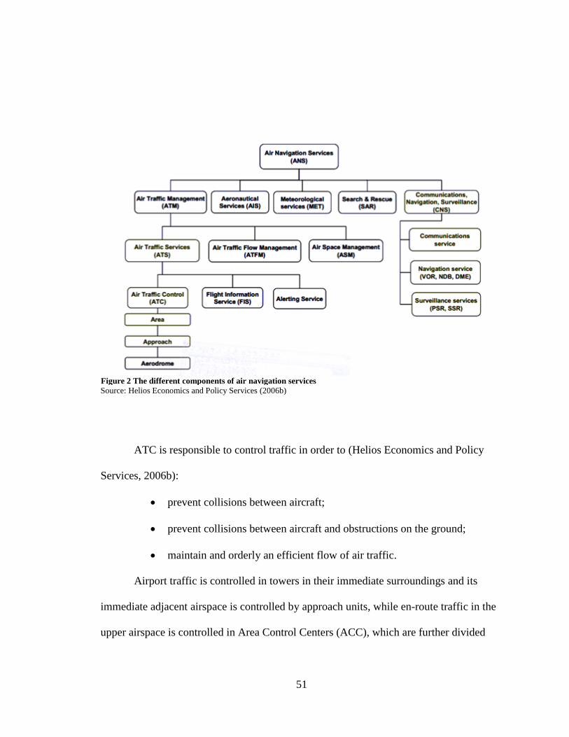
51

Source: Helios Economics and Policy Services (2006b)

ATC is responsible to control traffic in order to (Helios Economics and Policy

Services, 2006b):

prevent collisions between aircraft;

prevent collisions between aircraft and obstructions on the ground;

maintain and orderly an efficient flow of air traffic.

Airport traffic is controlled in towers in their immediate surroundings and its

immediate adjacent airspace is controlled by approach units, while en-route traffic in the

upper airspace is controlled in Area Control Centers (ACC), which are further divided

Figure 2 The different components of air navigation services

52

into en-route sectors, which have at least one air traffic controller (ATCo) manning each

one of them. These ATCos use a range of technological facilities, including radar and

satellite based location equipment, and air/ground communication equipment to safely

locate and separate traffic.

In terms of regulation, air traffic management procedures are regulated

internationally by ICAO, under “Doc 4444, Procedures for Air Navigation Services – Air

Traffic Management”, with Europe having a special setting of specific procedures,

published in “Doc 7030, Regional Supplementary Procedures” (Cook, 2007).

4.2. Commercialization and Privatization

Similar to the case of airports, ANSPs also began a transition in the 1980’s,

although at a much slower pace, towards different forms of regulation and ownership.

Also like airports, they had traditionally been operated directly by governments, which

under the Chicago Convention have sovereignty over the airspace in their territory and

the responsibility, “so far as it may find practicable” (article 28), to ensure that the

airspace is served by air traffic control. That did not mean, however, that governments

have to directly provide the services. They could be delegated, for example, to a firm

(like in Canada) or a supranational authority like EUROCONTROL. Now, there are a

range of different ownership structures and different types of regulation schemes (Button

& McDougall, 2006). This trend has become known as the “commercialization”99

of

ANSPs.

99

According to mbs ottawa (2006, p. 16), commercialization is “the range of organizational options and

regulatory frameworks that introduce business practices into what is, or traditionally was, the province of a

government department” , with “corporatization” and “privatization” being “considered as options within

53

From an operational viewpoint100

, commercialization was seen as needed due to a

number of factors. First, the issue of financing and budgets constraints, as ANSPs were

generally dependent on government budget for their capital and operational expenses, and

there was need for them to be able to generate their own revenue, either by charging for

their services, or by incurring into debt. Second, the issue of the need to become a

customer-oriented industry, serving their customers, i.e., the airlines, first, not the

governments and their lobbies or the unions, and to be free to establish their own

agendas. Finally, a range of other issues that derive from the fact of being part of the

government bureaucracy, from difficult, expensive, and slow procurement problems, to

difficulties in implementing new technologies, and labor issues. From this perspective,

commercialization can be considered a success, as most commercialized ANSPs, even

those 100% government-owned, have at least some level of independence from their

national governments. However, many non-commercialized ANSPs have achieved the

same level of independence, for example in terms of financing101

or safety regulation102

,

without having to leave the umbrella of their respective governments, so it might be

argued that greater levels of independence could happen in the industry regardless of the

underlying organizational structure.(Button & McDougall, 2006; Charles & Newman,

1995; Majumdar, 1995; United States Government Accountability Office, 2005)

the umbrella concept of commercialization”, and that an essential condition of the definition of

commercialization is “the introduction of some form of financial autonomy into the ANSP”.. Another,

similar, definition is provided by the United States Government Accountability Office (2005, p. 1):

“commercialization is the ability of an organization to operate like a commercial business”. 100

Commercialization can also be seen from an ideological or political perspective; also, the issues

regarding the rationale for the privatization of airports discussed in a previous chapter also apply here. 101

For example, the French ANSP is still a state agency but nevertheless has the authority to go to the

financial markets to finance itself. 102

Most countries now have separate agencies to regulate safety that are totally independent from their

ANSPs, even if they are still governmental agencies.

54

Commercialization of ANSPs began in New Zealand in 1987 with the creation of

a state-owned enterprise that pays dividends to the state. This was part of an overall

package of commercialization of state-owned enterprises in the country and led the way

to the other systems. Australia followed suit the next year (it was again re-structured in

the mid-1990’s), but the real impetus of commercialization took place in the late 1990’s

with the privatization of NAV Canada, the Canadian ANSP, along with the

commercialization of many European systems (Oster & Strong, 2007). This Canadian

privatization process, which had the support of the labor unions103

, began in 1994 and

concluded in 1996 with the creation of a non-share, not-for-profit corporation that is able

to charge user fees104

. The corporation has a board of directors that represent the four

stakeholders of the system: air carriers, general aviation105

, federal government, and

employees.

A number of other ANSPs have been commercialized since then, with most of

them becoming 100% state-owned corporations (for an overview of characteristics of

selected ANSPs see Table 2106

). These corporations do not have profit-maximizing goals,

being normally considered to be not-for-profit corporations, which might amount to a de

facto rate-of-return regulation. A major exception to this rule, and in fact a unique case

worldwide, is National Air Traffic Services Ltd (NATS), the British ANSP, which in

103

According to Oster and Strong (2007), labor pushed for privatization because they had not been given

pay rises for over six years and they had no right to strike. 104

Including in flights that only overpass the Canadian airspace and which previously were able to do so

for free. 105

General aviation is a term that encompasses all the non-commercial and non-charter flights (private jets,

recreational users, etc.). 106

For a more detailed analysis of a number of selected commercialized refer to the studies mentioned in

Chapter 5.

55

2001 became the only for-profit private ANSP107

. It operates under a PPP scheme where

51% of the shares belong to the private sector and the remaining 49% to the state.

Besides the form of ownership, NATS has also one characteristic that sets it apart from

its peers: the form of regulation. Under the PPP agreement, charges are subjected to a

price-cap regulation using the CPI-X method108

, inflation minus a factor to account to

productivity, normally a positive X, in order to create an incentive for increases in

productivity109

. In the first year of operation (2001) X was set a 2.2%, 4% in 2002, and

5% in the following years (Oster & Strong, 2007). In the current 2011-2014 period,

charges are expected to decline at an average rate of 1.44% per year (Civil Aviation

Authority, 2011b). 110

107

NATS is in fact a holding that included not-for-profit and commercial arms. The part of the company

that provide air traffic control services, NATS (En Route), is operating in a “not for commercial profit”

basis. 108

These charges are set by the Regulatory Policy Group of the UK Civil Aviation Authority. Charges are

usually set for five years, but that time-frame can vary (EUROCONTROL Performance Review

Commission, 2012). 109

The formula is quite more complicated nowadays, see “Condition 21” at Civil Aviation Authority

(2011a) for more details. Even at the beginning it also included a parameter related to quality of service, in

order to try and prevent the ANSP to reduce costs exclusively by reducing quality of service. 110

Chapter 7.2.3 will include more details on NATS. See also Goodliffe (2002) and Steuer (2010). For

more current regulatory information see the Civil Aviation Authority website at www.caa.co.uk.

56

Table 3 Basic features of selected air navigation service providers

Country ANSP Name Ownership Rate Regulation

Australia Airservices Australia Government corporation Commission oversight

Canada NAV CANADA Not-for-profit private

corporation

Legislated

principles/appeals

EUROCONTROL Maastricht Upper Area

Control Centre (MUAC)

International

organization

EUROCONTROL

Permanent

Commission

France Direction des services de la

navigation aérienne (DSNA)

State Agency Approved by transport

ministry

Germany Deutsche Flugsicherung

GmbH (DFS)

Government corporation Approved by transport

ministry

Ireland Irish Aviation Authority Government corporation Commission oversight

Netherlands Luchtverkeersleiding

Nederland (LVNL)

Government corporation Approved by transport

ministry

New Zealand Airways Corporation of New

Zealand

Government corporation Self-regulating/appeals

Switzerland Skyguide Government corporation Approved by transport

ministry

UK NATS Ltd. Public-private

partnership

Price capping

US FAA’s Air Traffic

Organization

State agency Financing from

taxation Notes: All ANSPs are financed by user fees except for the US Federal Aviation Administration that is funded by

taxation.

Source: Button and McDougall (2006) and EUROCONTROL Performance Review Commission (2013a).

4.3. Current Developments

4.3.1. Europe – Single European Sky

While sharing a similar geographical area, the US has only one single ANSP, the

Federal Aviation Administration (FAA), while Europe has several dozen. Despite the

similarity in size, the European system handles fewer flights, uses more centers and

airports, and is more labor intensive than the American system to which it is often

compared (Table 4)111

. Although there might be a number of technical reasons that can

111

Golaszewski (2002) outlines the nature of the US air navigation system and gives a comparative analysis

of the interactions between ANSPs and airport regulations in the US and Europe.

57

explain the differences, a particular issue is the lack of coordination across the European

systems, and that the small scale of many of the national European systems prevents

economies of scale from being exploited.

Table 4 US and European Air Navigation Systems (2012)

Europe US

Difference:

US vs. Europe

Area (million km2) 11.5 10.4 –10%

Number of air service navigation providers 37 1

Number of air traffic controllers 17,200 13,300 –23%

Total staff 58,000 35.500 –39%

Controlled flights (million) 9.5 15.2 +59%

Share of flights to/from top 34 airports 67% 66% -

Share of general air traffic 3.9% 21% x 5.4

Flight hours controlled (million) 14.2 22.4 +59%

Relative density (flight hours per km2) 1.2 2.2 x 1.8

Average length of flight (within respective

airspace) 559NM 511NM –11%

Number of en-route centers 63 20 -42

Number of approach control units (Europe)

and terminal facilities (US) 260 162 -98

Number slot controlled airports >90 4

ATM provision costs (billions of €2011) 8.4 7.8 -12% Note: NM is nautical miles

Source: EUROCONTROL Performance Review Commission & US Federal Aviation Administration (2013)

This fragmentation of the airspace112

, with its boundaries mimicking the national

borders on land (Figure 3) and frequent handing-over of traffic, is estimated to have

significant impacts on the overall efficiency of the system and its costs. This has resulted

in a an estimated €4.0 billion in annual delay costs in 2011, significant environmental

damage, and flights that are, on average, 49 km longer that they would need to be if the

112

Fragmentation can be defined as having operational units that are smaller than what is the operational

optimum, and as such this could happen not only because different national ANSPs are involved, but even

within a single ANSP.

58

airspace was optimized and more modern technologies were utilized (European

Commission, 2012b)113

.

A report commissioned by EUROCONTROL (Helios Economics and Policy

Services, 2006b) found out that fragmentation result not only from un-optimized

subdivision of airspace, but also from fragmented planning, piecemeal procurement, and

113

There is also a wide dispersion in the size of ANSPs, with the five largest European ANSPs handling

54% of the traffic and incurring 60% of the costs, with the remaining 46% of the traffic being handled by

over 30 different providers (EUROCONTROL Performance Review Commission, 2013a).

Figure 3 Flight information regions in European airspace

Source: www.eurocontrol.int

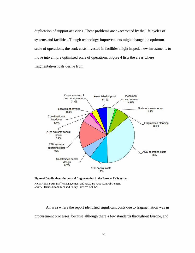
59

duplication of support activities. These problems are exacerbated by the life cycles of

systems and facilities. Though technology improvements might change the optimum

scale of operations, the sunk costs invested in facilities might impede new investments to

move into a more optimized scale of operations. Figure 4 lists the areas where

fragmentation costs derive from.

Note: ATM is Air Traffic Management and ACC are Area Control Centers.

Source: Helios Economics and Policy Services (2006b)

An area where the report identified significant costs due to fragmentation was in

procurement processes, because although there a few standards throughout Europe, and

Figure 4 Details about the costs of fragmentation in the Europe ANSs system

60

more are being developed, national, and sometimes even regional, idiosyncrasies in their

implementation means that the costs of development are higher, thus leading to higher

implementation costs. If there were a set of European-wide common procurement

specifications for technologies, there is a potential for significant cost reductions.

Planning investment appraisal is also identified as having considerable

importance in terms of increased costs. This is because this type of activity is done at the

national level, without concerns about how it affects the overall efficiency of the system.

Examples of this are the duplication of investments that could be done transnationally

with a better cost-benefit, and perpetuation of the existence of non-interoperable systems

across ANSPs, even after several product life-cycles where the issue could have been

addressed when updating those systems.

As a summary, the report concludes that there is no indication that fragmentation

significantly impacts either on safety or capacity; it simply increases the costs of

providing those levels of safety and capacity.

It is against this background that the European Commission created the Single

European Sky initiative with the aim of treating upper European airspace as a single

entity instead of being a patchwork of all the different national systems, thus creating a

European-wide Upper Information Region (UIR)114

. Unlike NextGen in the US115

, which

is mostly a technological initiative, SES includes not only technological initiatives, but

also policy and regulatory ones. Because of the complexity of the systems, their diversity,

114

UIRs are simply FIRs that only control the upper parts of airspace. 115

Discussed in Chapter 4.3.2.

61

and the inability to simply undergo a “big bang” style reorganization, a phased approach

to reform was initiated,

First proposed by the European Commission in 1999116

, the SES was put into law

in 2002 with enactment in 2004117

. It made ANSs a responsibility of the European Union

instead of its individual member states and has the main goal is improving the efficiency

and the capacity of ANSs in Europe. This is intended to be done by promoting airspace

restructuring and rationalization, consolidation of facilities, and harmonization of systems

and procedures (Helios Economics and Policy Services, 2006b). A number of stipulations

were put in place by legislation in both 2002 and 2009, including the creation of the

Functional Airspace Blocks (FABs), the Single European Sky ATM Research (SESAR)

technological initiative to modernize the ANS system118

, and the extension of

competencies of the European Aviation Safety Agency (EASA) to include air traffic

management and air navigation services119

(European Commission, 2012a).

One of the fundamental aspects of the SES initiative are the FABs, which have

the goal of reducing the inefficiencies – in terms of safety, capacity, and cost – that result

from the fragmentation of European airspace120

. FABs are seen as an explicit bottom-up

116

At the time, a High-Level Group was formed by the European Commission to study the issue. 117

Implementation involves a number of institutions and initiatives involving; the European upper

information region (EUIR), functional airspace blocks (FAB), flexible use of airspace (FUA), National

Supervisory Authorities (NSA), certification of ANSPs, air traffic controllers licensing, interoperability,

SESAME, and extensions to third party countries. 118

SESAR could be considered as the European counterpart of US’ NextGen. 119

Essentially forcing the separation of provision and safety oversight for the systems that have not done so

already. 120

The criteria for the creation of FABs are strictly to do with:

• safety;

• optimum use of airspace, taking into account air traffic flows;

• overall added value, including optimal use of technical and human resources, on the basis of CBA;

• ensuring a fluent and flexible transfer of responsibility for air traffic control;

62

approach to the ultimate integration of European airspace.121

They seek to improve ANS

for a number of national airspaces by better coordination of their ANSPs. The underlying

philosophy being that, “each FAB is different and faces different political, operational,

technical, and economic challenges. (…) FAB initiatives show wide differences in scope,

timescales and approaches. It is clear that a flexibility of approach needs to be

maintained, as long as improvements are delivered.” (EUROCONTROL Performance

Review Commission, 2008, p. v).

The concept was established in 2002 in the first SES legislative package and

further developed in 2009 in the second legislative package, the so-called SES II

(European Commission, 2012b). The initial idea was that they were to be based on the

experience of States/ANSPs when being set with the European Commission developing

binding general principles for establishment and modification of FABs. The extension of

FABs to lower airspace below 28,500 feet was to be studied by the Commission before

the end of 2006, with the Commission reviewing the functioning of the bottom-up

approach by early 2009 and to propose additional measures, if necessary. The aim was

that by 24 June 2012, the consultation material of all FABs shall be submitted to the

European Commission, a target that was not met.

• ensuring compatibility between upper and lower airspace;

• complying with regional agreements concluded within ICAO;

• respecting regional agreements, in particular those involving European third countries. 121

Strictly a FAB is defined in the SES legislative package, namely Regulation (EC) No. 1070/2009

amending Regulation (EC) No. 549/2004, as an airspace block based on operational requirements and

established regardless of State boundaries, where the provision of air navigation services and related

functions is performance-driven and optimized through enhanced cooperation among ANSPs or, when

appropriate, an integrated provider (European Commission, 2012a).

63

The phasing in of the SES is almost inevitable, but there are often issues when

changes are made sequentially rather than as a single “big bang”122

. In particular, major

changes often occur when there is a crisis in the existing regime and a consensus, or at

least a dominant coalition of interests emerge for change; it is also useful to have what is

seen as a more favorable alternative available. A comprehensive, rapid change, while

often painful to many parties in the short-term, yields subsequent positive results for the

system as a whole at about the same time. Gradual changes often affect different groups

differently during the change, leading to reluctance for some parties to move forward. Ex

ante, those likely not to be early winners are often reluctant participants. The SES

initiative inevitably entails differential changes by the various ANSPs at different times,

leading to the potential of simply moving from one sub-optimal situation to another and

remaining stuck there123

.

With the FABs, operational concerns would supersede national boundaries in the

handling of traffic. The rationale behind this is that it will lead to an optimized use of the

airspace and will facilitate the handing out of traffic between operators, thus reducing the

inefficiencies of the system. To be established, the proposed FABs have to report to the

European Commission on a number of topics, including safety, consistency with

European Union-wide performance targets, and be justified by their overall added value,

on the basis of cost-benefit analyses (CBA) (European Commission, 2012a).

122

As discussed in Chapter 3.3.1, one can compare the different ways in which airline deregulation was

approached, with the US basically adopting a big-bang approach, and the EU adopting the “three packages”

staged approach over a decade. 123

A similar situation is occurring with the NextGen technological initiative that aims to improve ANS in

the United States. It is also been implemented in a staged approach, and like in Europe many stakeholders

(namely airlines) have also been reluctant to jump in, fearing that the realized gains will take too long to

materialize. Next Gen will be discussed in Chapter 4.3.2.

64

Nine FABs have been proposed, but only the first two have been declared

established and notified to the European Commission124

:

UK-Ireland FAB

Danish-Swedish FAB

Baltic FAB (Lithuania, Poland)

BLUE MED FAB (Cyprus, Greece, Italy and Malta)

Danube FAB (Bulgaria, Romania)

FAB CE (Austria, Bosnia & Herzegovina, Croatia, Czech Republic,

Hungary, Slovak Republic, Slovenia)

FABEC (Belgium, France, Germany, Luxembourg, the Netherlands and

Switzerland)

North European FAB (Estonia, Finland, Latvia, and Norway)

South West FAB (Portugal, Spain).

Figure 5 shows the FABs in their geographical context, and Table 5 presents some

basic statistics relating to the individual ANSP aggregated at the FAB level.

Table 6 presents the financial and economic KPIs125

for the FABs as estimated by

EUROCONTROL for the year 2011.

124

All the FABs produce periodic reviews of progress that contain quasi CBA of their activities,

embracing some environmental as well as operational performance assessments e.g. for the UK-Ireland

FAB, see Irish Aviation Authority & NATS (2012). These contain performance data, but no rigorous

assessment of economic efficiency. 125

Key Performance Indicator. These are a measure of performance estimated by EUROCONTROL, with

lower being better. More details are discussed in Chapter 5.

65

.

Figure 5 The functional airspace blocks.

Source: www.eurocontrol.int

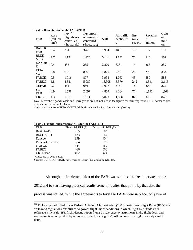
66

Table 5 Basic statistics of the FABs (2011)

FAB

Area

(million

km2)

IFR126

flight-hours

controlled

(thousands)

IFR airport

movements

controlled

(thousands)

Staff

Air traffic

controller

s

En-

route

sectors

Revenues

(€

million)

Costs

(€

milli

on)

BALTIC

FAB 0.4 394 326 1,994 486 10 172 171

BLUE

MED 1.7 1,751 1,428 5,141 1,992 78 940 994

DANUB

E 0.4 453 255 2,800 635 14 265 250

DEN-

SWE 0.8 606 836 1,825 728 28 295 333

FABCE 0.5 1,016 807 3,933 1,063 43 589 586

FABEC 1.8 4,581 5,080 16,908 5,370 242 3,341 3,115

NEFAB 0.7 431 686 1,617 513 18 200 221

SW

FAB 2.9 1,598 2,097 4,859 2,064 77 1,191 1,168

UK-IRE 1.3 1,511 1,911 5,029 1,608 82 925 846

Note: Luxembourg and Bosnia and Herzegovina are not included in the figures for their respective FABs. Airspace area

does not include oceanic airspace.

Source: adapted from EUROCONTROL Performance Review Commission (2013a).

Table 6 Financial and economic KPIs for the FABs (2011)

FAB Financial KPI (€) Economic KPI (€)

Baltic FAB 315 384

BLUE MED 423 547

Danube 399 404

Denmark-Sweden 364 378

FAB CE 444 489

FABEC 466 566

UK-Ireland 462 424 Values are in 2011 euros.

Source: EUROCONTROL Performance Review Commission (2013a).

Although the implementation of the FABs was supposed to be underway in late

2012 and to start having practical results some time after that point, by that date the

process was stalled. While the agreements to form the FABs were in place, only two of

126

Following the United States Federal Aviation Administration (2008), Instrument Flight Rules (IFRs) are

“rules and regulations established to govern flight under conditions in which flight by outside visual

reference is not safe. IFR flight depends upon flying by reference to instruments in the flight deck, and

navigation is accomplished by reference to electronic signals”. All commercials flights are subjected to

IFRs.

67

them (DEN-SWE and UK-IRE) have been declared established and notified to the

European Commission, and the consolidation of air traffic control has yet to take place

(European Commission, 2012b).127

Another way in which the European system is changing is in the way it collects

charges for ANSs. Charges are collected for both airport movements, i.e., landings and

departures, and en-route, i.e., while the plane is in flight. Charges, which account for

around 6% of the prices of airline tickets in Europe, are set a national level, but they are

regulated at the European level. Until recently, under Regulation (EC) 1794/2006,

European regulations imposed full cost recoveries mechanisms, in which any shortfalls in

revenue lead to charges going up, and any profits had to be redistributed back to the

airspace users (Casteli et al., 2012).

This charging scheme created two perverse effects. One, when traffic is declining,

rates have to go up, potentially exacerbating the problem. Two, any productivity and

efficiency increases to lead to increase profits had to be returned in full to the airspace

users, thus reducing the incentives for good management and procedures. To change this

paradigm, Regulation (EC) 1191/2010 was published. Under this new scheme two new

concepts were introduced: a traffic risk sharing mechanism that tries to mitigate

unexpected increases in costs or declines in traffic128

, and financial penalties or bonus for

productivity and efficiency changes are now allowed. In practice, this will result in a

system were costs do not have to be fully recovered each year, and it will also allow

127

For example, the two FABs already established still maintain separate rates for each of the ANSPs that

are part of them (Casteli et al., 2012). 128

A scheme already in use in the regulated arm of UK’s NATS.

68

ANSPs to keep at least a portion of eventual profits. This new regulatory framework was

started to be implemented in 2012, and should finished by 2014 (Castelli et al., 2012).

4.3.2. United States – NextGen

Efforts to modernize the technology in use at the FAA129

have been recurrent for

decades. In the late 1980’s, the FAA started the implementation of the Advanced

Automation System (AAS), which aimed at increasing capacity by completely revamping

the hardware and software system in place at the FAA, including a major consolidation of

facilities and the introduction of many automated capabilities. However, the program in

its entirety never came to fruition, and only a few of the planned improvements were

implemented, a total of $1.5 billion were spent, with estimates that around two-thirds of

that investment was wasted, and only the remaining $500 million did anything to improve

the ANSs system (Office of Inspector General, 1998).

More recently, in 2004, a new plan was envisioned: the Next Generation Air

Transportation System, now simply marketed as NextGen. With this plan, which shares

some similarities with the SESAR program being implemented in Europe, by the mid

2020’s the US ANSs system will move from the current ground radar-based control

system, to a satellite-based one. For the most part, the need for this comes from capacity

and cost concerns. The current system relies on expensive ground infrastructure that is a

legacy from World War II-era technology, and the move to satellite based control would

increase accuracy, thus allowing controllers to squeeze more planes into the same

129

This chapter will analyze US’ ANSs mainly from a technological perspective. For an institutional

treatment see the US’ case study in Chapter 7.2.4.

69

airspace and increase capacity this way – a must, given predictions that traffic will double

or triple in the next two decades. This is mainly due to the implementation of Automatic

Dependent Surveillance – Broadcast (ADS-B), a system, already implemented in Alaska

and the Gulf of Mexico130

that allows airplanes to be aware of the traffic around them

without having to rely on information transmitted to them by ATCos. Moving to a

satellite-based system also makes possible, or at least more feasible, other enhancements

like “free flights”/4-D trajectories in which the airplanes follow direct routes between two

points instead of relying in the series of ground-based waypoints they have to follow with

the current system (Federal Aviation Administration, 2013; Oster & Strong, 2007).

Implementation has been the major concern with NextGen for two reasons: cost

overruns and equipage. The AAS experience had shown the risks of trying to implement

such large scales projects, and the fiscal situation in the US combined with the reliance of

the FAA from Congress appropriations makes implementation difficult and cost overruns

could happen (Table 7). In terms of equipage, the risk is that until most if not all airspace

users make the necessary investments to equip their airplanes the lowest common

denominator, in terms of separation, for example, must be adopted to maintain safety

levels. This leads to a situation where airspace users are not eager to make the necessary

investments to equip their airplanes while knowing that many of the benefits in terms of

savings will take a long time to materialize and will only come when a majority of users

has adopted the technology.

130

And that will be mandatory for most airplanes in both Europe and the US by the end of the decade.

70

That concern has lead Robyn (2007) to suggest that the implementation should

move from the current “big bang” approach that would deliver significant results only

when all new systems are put in place, which should happen by mid-2020’s, to a more

staged approach that would start to deliver benefits sooner, thus increasing the incentives

for airlines and other stakeholders to take part in the process.131

131

The United States Government Accountability Office has been producing a number of reports on the

challenges in implementing NextGen. See, for example, United States Government Accountability Office

(United States Government Accountability Office, 2010a, 2010b, 2011a, 2011b, 2012a, 2012b, 2013).

Table 7 Selected NextGen projects with cost and schedules performance

Costs in millions of dollars.

Source: United States Government Accountability Office (2012b)

71

CHAPTER 5 – BENCHMARKING AIR NAVIGATION SERVICES:

LITERATURE REVIEW

With the commercialization efforts that have been underway in many systems, the

efficiency of ANSPs has also been attracting some attention in the literature. The number

of published research is not near as extensive as the one dealing with airport efficiency

though, and the scope is also normally quite different, with most of them being case

study-like approaches, with little in-depth economic analysis. The reasons for this “lack

of interest” might have several explanations, from unavailability of data, the relative

recentness of the changes in many systems, or simply because ANSPs and air traffic

control do not draw as much attention as airports and airlines.

EUROCONTROL has been one of the most active in producing benchmarking

studies, and for the last 15 years they have had a department, the EUROCONTROL

Performance Review Commission132

, that has been publishing a number of reports a part

of their mission to monitor performance and propose targets for improvements. These

reports include the annual “ATM Cost-Effectiveness (ACE) Benchmarking Report” (with

EUROCONTROL Performance Review Commission, 2013a being the most recent),

hereafter referred as ACE, and the also annual “Performance Review Report” (with

EUROCONTROL Performance Review Commission, 2013b being the most with),

hereafter referred as PRR.

132

For the history on how and why the Performance Review Commission was created see McInally (2010).

72

The ACEs provide a number of performance indicators relating to cost-

effectiveness and productivity, the analyses of past trends, and forecasts for the future.

This analysis in conducted at the European level and also at the individual ANSP level.

The main outputs of this report are the “financial gate-to-gate cost-effectiveness KPI” and

the “economic gate-to-gate cost-effectiveness KPI”133

, with the latter being the former

plus measures of air traffic control-induced delays. There are also a number of

intermediate indicators (employment costs, provision costs, capital expenditures,

productivity levels, etc.) that are used in the calculation of these KPIs.

In terms of financial cost-effectiveness, a “composite flight-hour”134

in 2011 cost

an average of €423 in Europe, with a wide variation of cost among ANSPs, from €175 in

Estonia to almost €700135

in Belgium, four times more. Analyzing the evolution along the

years, costs in real terms have decreased a modest 0.2% per annum between 2007 and

2011. Looking into more detail, it can be seen that in 2009 costs have increased 8.7% in

real terms compared to 2008, followed by a decreased of 6.8% the next year and a further

decline of 2.1% in 2011. This is most likely a result of the decrease in traffic that resulted

from the 2008 financial crisis. Since the ANSPs did not have time to adjust and

maintained a structure that was ready for a certain level of traffic, the decline in traffic

lead to increased costs per flight, and in the next year, they started to adjust to the new

133

For a discussion of the development of these indicators see EUROCONTROL Performance Review

Commission (2001). 134

This is a composite measure created by EUROCONTROL that takes into account both airport

movements and actual flight-hours, in order to allow for the creation of a single performance measure

(EUROCONTROL Performance Review Commission, 2012). 135

All these monetary values are not adjusted for the different purchasing power in each country. The

reports have more info on how monetary issues – exchange rates and purchasing power parities – are dealt

with.

73

traffic levels, and thus a steep decline in costs followed. The latest report included some

analysis at the FAB level. Levels of dispersion are half of what they are at the individual

level, with the financial KPI ranging from €315 (Baltic FAB) to €466 (FABEC).

As for economic cost-effectiveness, the European average for 2011 was €502 per

composite flight-hour, also with the same levels of variation, although with the added

variable, of having ANSPs in which delays are almost non-existent136

and other in which

delays are a considerable part of the cost137

. The evolution along the years shows a 0.8

decrease in real terms per annum since 2007, but this all results of a sharp decline of

10.2% from 2010 to 2011, as in the four years prior there had been an increase every year

that totaled 7% in real terms. As there was a decrease in the financial cost-effectiveness

during the same period, all of this increase can be attributed to an increase in the costs

associated with delays, but in the last year, a large decline in the amount of delays

reported brought the KPI down 10.2%. At the FAB level, dispersion is also much smaller

like it was in the case of the financial KPI, ranging from the €375 per composite-hour of

NEFAB to €602 per composite-hour of the South West FAB. Table 8 presents the values

for the financial and economic KPIs for 2011 for the individual ANSPs, and Table 9138

the same values for the FABs. Table 10 presents the performance ratios139

for the

individual components that are used to estimate the financial KPI, along with

employments costs per hour.

136

Malta, Slovenia, Romania, etc. 137

Cyprus or Greece, for example, with the latter being the most extreme example, where taking delays into

account inflates the price per composite flight-hour from €303 to more than €701, more than double. 138

This is the same table as Table 6. 139

Defined as being the relationship between the value for an ANSP of an indicator and the value for the

entire European system – i.e., values greater than one (the European average) indicate that particular ANSP

performs better than average on that indicator, and vice-versa.

74

Table 8 Financial and economic KPIs for the individual ANSPs (2011)

ANSP Financial

KPI (€)

Economic

KPI (€) ANSP

Financial

KPI (€)

Economic

KPI (€)

Albania 414 581 Latvia 253 253

Armenia 357 357 Lithuania 350 350

Austria 469 555 Malta 248 248

Belgium 699 748 Moldova 377 377

Bulgaria 366 379 Netherlands 589 725

Croatia 357 456 Norway 383 420

Cyprus 250 507 Poland 310 388

Czech Rep. 441 448 Portugal 374 405

Denmark 367 376 Romania 419 419

EUROCONTROL 229 238 Serbia 354 364

Estonia 175 180 Slovakia 549 549

Finland 316 389 Slovenia 513 514

France 436 496 Spain 479 640

FYROM 454 454 Sweden 363 379

Germany 499 677 Switzerland 600 713

Greece 303 701 Turkey 283 336

Hungary 429 430 UK 385 430

Ireland 385 386 Ukraine 586 586

Italy 495 505

Values are in 2011 euros.

Source: EUROCONTROL Performance Review Commission (2013a)

Table 9 Financial and economic KPIs for the FABs (2011)

FAB Financial KPI (€) Economic KPI (€)

Baltic FAB 315 384

BLUE MED 423 547

Danube 399 404

Denmark-Sweden 364 378

FAB CE 444 489

FABEC 466 566

UK-Ireland 462 424 Values are in 2011 euros.

Source: EUROCONTROL Performance Review Commission (2013a).

75

Table 10 Performance ratios for the different components of the financial KPI and employment costs for the

individual ANSPs (2011)

Performance ratios

ANSP ATCO-hour

productivity

Employment

costs

per ATCO-hour

Support cost

per ATCO-hour

Employment

costs

per CFH

Support

costs

per CFH

Albania 0.72 3.63 0.39 2.62 0.81

Armenia 0.24 8.08 0.6 1.97 1.01

Austria 1.18 0.65 1.17 1.77 0.97

Belgium 0.88 0.78 0.88 0.69 0.58

Bulgaria 0.93 1.97 0.63 1.82 1

Croatia 0.84 1.22 1.16 1.02 1.27

Cyprus 0.91 1.85 1.01 1.68 1.7

Czech Rep. 1.17 1.11 0.74 1.29 0.86

Denmark 1.28 1.08 0.83 1.39 1.07

EUROCONTROL 2.45 0.65 1.17 1.58 1.99

Estonia 0.96 2.67 0.94 2.57 2.35

Finland 0.85 1.44 1.09 1.22 1.39

France 0.93 1.1 0.95 1.02 0.95

FYROM 0.28 3.57 0.92 1.01 0.9

Germany 1.29 0.66 0.99 0.85 0.84

Greece 0.94 1.28 1.16 1.2 1.5

Hungary 1.03 0.93 1.03 0.96 1

Ireland 1.2 1.07 0.86 1.28 1.04

Italy 0.91 0.95 0.99 0.86 0.85

Latvia 0.96 3.36 0.52 3.23 1.38

Lithuania 0.62 2.69 0.72 1.67 1.08

Malta 0.92 3.3 0.56 3.04 1.43

Moldova 0.29 8.36 0.47 2.39 0.91

Netherlands 1.19 0.74 0.81 0.88 0.66

Norway 0.99 0.87 1.28 0.86 1.25

Poland 1.22 1.05 1.06 1.29 1.4

Portugal 1.17 0.63 1.52 0.75 1.45

Romania 0.75 1.75 0.77 1.31 0.92

Serbia 0.96 2.01 0.62 1.93 1.02

Slovakia 0.83 1.38 0.68 1.14 0.68

Slovenia 0.58 1.24 1.15 0.72 0.88

Spain 0.99 0.62 1.45 0.61 1.09

Sweden 0.85 0.92 1.48 0.78 1.47

Switzerland 1.24 0.69 0.77 0.92 0.64

Turkey 1.01 2.39 0.62 2.41 1.28

UK 1.25 0.96 0.91 1.2 1.06

Ukraine 0.41 4.53 0.39 1.86 0.57

76

Employment costs (€)

ANSP Per

ATCO-hour Per CFH

Albania 28 49

Armenia 13 65

Austria 156 166

Belgium 130 185

Bulgaria 51 70

Croatia 83 125

Cyprus 55 76

Czech Rep. 91 98

Denmark 94 92

EUROCONTROL 157 81

Estonia 38 50

Finland 70 104

France 92 125

FYROM 28 126

Germany 154 149

Greece 79 106

Hungary 109 133

Ireland 95 99

Italy 106 147

Latvia 30 39

Lithuania 38 76

Malta 31 42

Moldova 12 53

Netherlands 136 144

Norway 116 147

Poland 96 99

Portugal 160 171

Romania 58 97

Serbia 50 66

Slovakia 73 112

Slovenia 82 178

Spain 164 209

Sweden 110 162

Switzerland 148 138

Turkey 41 53

UK 106 106

Ukraine 22 68

Performance ratios are relative to the system-wide average, monetary values are in 2011 euros.

Source: EUROCONTROL Performance Review Commission (2013a)

The PRRs expand on the ACEs by including not only analysis of cost-efficiency,

but also analysis of safety, capacity and delays, and environment and flight efficiency.

While the ACEs provide both a global analysis of the European ANSs system and an

77

individual breakdown of issues for every ANSPs, these PRRs have a much more global

focus, with almost all the analysis being done on an European-wide level.

The main findings in the last report in the three areas not covered by the ACEs

are:

In terms of safety, ANSs continue to not be a problem in Europe.

However, the report points out that a high number of incidents, probably

in the tens of thousands, remain unreported every year, and that policies

are needed to address that issue with every ANSP; this is specially the

case of Turkey and Ukraine which do not provide EUROCONTROL with

an annual summary of incidents, and some other countries also have

problems in data reporting;

As for capacity and delays, there have been positive improvements, with

delays accruing to 0.63 minutes per flight in 2012 – 11 years earlier it was

3.1 minutes per flight, and in 2011 it was still at 1.1 minutes. Thus, this

was the first year in which the target of 1 minute of delays per flight has

been achieved. As for delays at major airports, the levels of delay have

been stagnant in the last five years considered in the report;

From the environmental and flight efficiency perspective, which is

measured by comparing the direct route between origin and destination,

and the actual route that airplanes have to fly, there has been an increase in

efficiency, albeit rather modest: in 2009 on average flights were 3.5%

bigger than they needed to be – i.e., for every 100 kilometers of direct

78

path, planes had to fly 103.5 kilometers –, as value that had decreased to

3.2 kilometers in 2012. This figure is affected significantly by exogenous

factors, be it natural disasters, like the Icelandic volcano eruption of 2010,

or other things like industrial actions – strikes – or military exercises that

make planes to have to re-route and deviate from the most direct flight

path.

Besides these annual endeavors, EUROCONTROL has published a few more

studies, including a TFP analysis (EUROCONTROL Performance Review Commission,

2005b) , an econometric stochastic frontier analysis (Competition Economists Group,

2011), and comparisons with the North-American system (EUROCONTROL

Performance Review Commission & Federal Aviation Administration, 2009, 2012, 2013;

EUROCONTROL Performance Review Commission, 2005a; EUROCONTROL, 2013).

The TFP report analyzed the performance of 29 European ANSPs in the three-

year period from 2001 to 2003. The results showed an overall increase of 2% of the

productivity levels over the period, but the individual analysis of ANSPs showed

variations from -21 to +37 percent. Comparing the results of this study with the partial

productivity indexes of the ACEs showed high levels of correlation, with a R2 of 0.74.

The more recent econometric SFA study140

applied a cost function with a Cobb-

Douglas specification with the inclusion of several explanatory variables, ranging from

operational factors to socio-economic conditions of each individual countries – one

140

Before this study, NERA (2005) also used a SFA framework to compare the efficiency of European

ANSPs between 2001 and 2004, but due to lack of data, results were considered to be poor, and no major

conclusions were drawn.

79

variable that was not included, though, was the ownership status of the ANSP. Results

from the different models tested showed an average level of inefficiency ranging from 13

to 60%, with the authors concluding (p. 25) “It is likely that the “real” level of

inefficiency is within the threshold provided by these two different models”. Other

findings include the presence of economies of scale in the provision of ANSs, and that

the “quality of the business environment”, a variable which (p. 16) “reflects the risk to

invest in a given country taking into account the local business and institutional

environments” is associated with lower costs of provision.

The comparisons with the situation in the US are useful because of the differences

between the two systems (Table 4, previous chapter). While the United States has a single

system to control 10.4 million km2 and almost 16 million annual flights, in Europe,

almost 40 systems control an area that is only slight larger and has much fewer flights in

it – less than 10 million in fact.

Besides discussing differences in how the systems conduct operations, these

reports have shown that while ATCos in the US control more flight-hours per annum,

that is offset by higher labor costs, making the levels of labor productivity similar.

Regarding delays provoked by the ANSs system, the reports found that the total amounts

of delays attributable to them are similar in both cases, but the stage of flight when these

delays occur are different. In the US, they occur most often at the airports, due to the

levels of congestion at those airports and over-scheduling of flights by airlines. In

Europe, they happen during the flight because of the fragmentation of the European

airspace that leads to less-optimal routes. In terms of costs, they have increased at greater

80

rates in the US compared to Europe, with provision costs being 35% higher in real terms

in 2011 when compared to 2002 in the US, while they were only 21% higher in Europe

for the same period of time. This evolution meant than while in 2002 costs per flight-hour

were 55% lower in the US, by 2011 they were only 34% lower.

More recently than EUROCONTROL, the Civil Air Navigation Services

Organisation (CANSO), an international industry association of ANSPs, has also begun

to benchmark some aspects of its members’ operational efficiency. So far, three reports

have been released (CANSO, 2010, 2011, 2012).

These reports cover the operations of around 30 ANSPs around the world in five-

year periods: 2005-2009 in the 2010 study; 2006-2010 in the 2011 one; and 2007-2011 in

the 2012 study. The main interest of these reports is the inclusion of systems that are

normally not studied as much, like the ones from Mexico, Dubai, Thailand, or South

Africa; however, the ANSPs included vary between the reports, and some of them are

included in the older reports and not in the most recent. Even within each report, there are

variations in the ANSPs that are included in each study undermining the usefulness of the

reports for a more thorough long-term analysis141

.

The main outcomes of the reports are three indicators: flight-hours per controller,

costs per flight-hour, and revenues per flight-hour, which are measures of productivity,

cost-effectiveness, and revenue, respectively. However, the reports do not present any

data on safety, air traffic complexity, or quality of service. All reports reach similar

141

This is also affected by the relative recentness of the reports and the consequent short span of data

availability.

81

conclusions: a recovery trend is present, but it remains fragile due to the uncertainties

regarding the global economy.

Table 11, Table 12, and Table 13 present some of the findings from the last

report in terms of productivity and cost-effectiveness along with some basic statistics

regarding these results. The results show the disparities in the levels of productivity and

cost-effectiveness achieved by the different ANSPs.

82

Table 11 IFR flight-hours per ATCo in operations (worldwide data)

ANSP

2007 ($) 2008 ($) 2009 ($) 2010 ($) 2011 ($)

Annual

average

change

Canada 1624 1733 1631 1613 1683 1.0%

Czech Rep. 1194 1240 1186 1223 1213 0.4%

Denmark 943 1158 1045 1066 1106 4.7%

Estonia 1792 1647 1326 1046 964 14.1%

Finland - - 559 591 660 8.7%

Georgia 376 362 347 384 363 -0.7%

Hungary 1072 1103 1144 1151 1119 1.1%

Ireland 1245 1269 1124 1210 1250 0.4%

Latvia 1022 1052 834 790 918 -1.7%

Mexico 1653 1529 1350 1394 1351 -4.8%

New

Zealand 814 872 802 747 718 -2.9%

Portugal 1397 1418 1290 1275 1422 0.7%

Romania 498 523 520 652 681 8.6%

Serbia 764 927 928 934 904 4.7%

Slovakia 658 715 689 824 875 7.7%

South

Africa 1161 1128 1080 969 884 -6.5%

Spain 740 720 649 730 748 0.6%

Sweden 812 881 784 767 775 -0.9%

UK 1028 1092 948 922 1081 1.9%

USA 1934 1995 1882 1902 1800 -1.7%

Average 1091 1124 1006 1010 1026 1.8%

Minimum 376 362 347 384 363 -6.5%

Maximum 1934 1995 1882 1902 1800 14.1%

Standard

deviation 423 406 371 353 346 4.9%

Monetary values are in 2007 dollars.

Source: CANSO (2012) and calculations by the author.

83

Table 12 Cost per IFR flight-hour (worldwide data)

ANSP

2007 ($) 2008 ($) 2009 ($) 2010 ($) 2011 ($)

Annual

average

change

Canada 358 344 344 352 340 -1.3%

Czech Rep. 743 718 732 735 697 -1.6%

Denmark 639 725 805 769 802 6.1%

Estonia 228 262 277 294 285 5.9%

Finland - - 776 738 691 -5.6%

Georgia 792 849 455 454 615 -1.0%

Hungary 412 491 611 756 791 18.0%

Ireland 542 573 607 647 687 6.1%

Latvia 431 452 498 569 501 4.3%

Mexico 97 108 126 123 125 6.9%

New

Zealand

323 325 357 378 396 5.3%

Portugal 730 780 763 660 648 -2.7%

Romania 781 882 905 811 824 1.7%

Serbia 581 563 625 710 794 8.4%

Slovakia 706 741 893 872 888 6.2%

South

Africa

263 282 307 369 434 13.5%

Spain 1117 1178 1291 972 910 -4.0%

Sweden 551 542 676 751 744 8.3%

UK 806 739 867 892 1000 6.0%

USA 336 363 403 425 433 6.6%

Average 549 575 616 614 630 4.4%

Minimum 97 108 126 123 125 -5.6%

Maximum 1117 1178 1291 972 1000 18.0%

Standard

deviation

247 257 270 224 227 5.7%

Monetary values are in 2007 dollars.

Source: CANSO (2012) and calculations by the author.

84

Table 13 Employment costs for ATCo in operations per IFR flight-hour (worldwide data)

ANSP

2007 ($) 2008 ($) 2009 ($) 2010 ($) 2011 ($)

Annual

average

change

Canada 103 103 111 114 113 2.3%

Czech Rep. 173 145 142 142 157 -1.9%

Denmark 181 169 232 232 188 2.8%

Estonia 51 70 70 70 84 15.0%

Finland - - 246 246 230 -2.9%

Georgia 39 49 51 51 61 13.0%

Hungary 114 124 150 150 239 21.4%

Ireland 144 156 177 177 175 5.2%

Latvia 65 69 69 69 74 3.4%

Mexico 25 27 35 35 39 12.4%

New

Zealand

110 112 129 129 149 8.0%

Portugal 200 240 263 263 296 11.1%

Romania 234 239 240 240 191 -4.3%

Serbia 109 100 112 112 135 5.9%

Slovakia 154 146 172 172 181 4.5%

South

Africa

41 50 60 60 97 24.5%

Spain 657 702 736 736 391 -10.0%

Sweden 159 202 255 255 304 18.2%

UK 194 186 241 241 243 6.5%

USA 88 86 94 97 102 3.7%

Average 150 157 179 180 172 6.9%

Minimum 25 27 35 35 39 -10.0%

Maximum 657 702 736 736 391 24.5%

Standard

deviation

133 142 147 147 89 8.5%

Monetary values are in 2007 dollars.

Source: CANSO (2012) and calculations by the author.

There have been at least two studies (mbs ottawa inc., 2006; United States

Government Accountability Office, 2005, the former analyzed 5 commercialized ANSPs,

and the latter 10 - the total number of commercialized ANSPs is close to 50 now ) that

have considered the issue of the commercialization of ANSPs. These studies concluded,

85

albeit from small samples, that changes were either neutral or positive, with

improvements in customer service, more modernization efforts undertaken, and that

financial stability was maintained, while costs were, in the worst cases, kept in check or

even reduced. McDougall & Roberts (2008) reported similar results. An older case study

(Majumdar, 1995) conducted when commercialization was in its infancy, examined two

at-the-time-recent commercialization processes (New Zealand and Germany) and other

two that were proposed at the time (UK and US, with only the former being successfully

commercialized since then). It concluded that the biggest risk of commercialization

would inevitable be safety, as the mindset of reducing costs under commercialized

ANSPs would put pressure on safety levels and ultimately (p. 122) "the debate is as to

how much 'less safe' can an operation be before it becomes 'unsafe'".

Other studies include a large overview of issues related to ANSPs (Oster &

Strong, 2007), in which some analysis of commercialization experiences are also

included142

; and a similar approach but with a focus on Europe and also a more detailed

technical analysis of ANSs (Cook, 2007), while others analyze the rationale behind

commercialization (Charles & Newman, 1995; Dempsey, Janda, Nyampong, Saba, &

Wilson, 2005; Morrison & Winston, 2008; Robyn, 2007).

Besides being studied with varied levels of depth in virtually every study

pertaining to ANSP commercialization, UK’s NATS have seen a number of publications

dedicated to this system, including academic papers (Goodliffe, 2002; Steuer, 2010) and

142

The book followed a report by the same authors about commercialization efforts in the UK and Canada

(Oster & Strong, 2006).

86

a plethora of regulatory policy analysis made public by UK’s Civil Aviation Authority143

.

The report by Helios Economics and Policy Services (2006a) may be the most relevant

for the scope of this dissertation.

There are still a number of issues that still have not been developed in the

literature. For example, pricing and pricing regulation also vary significantly across

ANSPs, from taxes on tickets (with the most notable case being the United States) to user

charges. Among user charges, those can be set independent civil aviation authorities, by

the respective governments, or being subjected to price-capping (as is the case of the

British ANSP, NATS), and are a subject that have deserved little or no research – an

exception being Castelli et al. (2012), although this is mostly a study about rate

optimization from a mathematical perspective, not from an economic/regulatory

standpoint. Issues like the role of disruptive events that change the predicted traffic

patterns (recessions, volcanoes, epidemics, etc.) in the economic efficiency of ANSPs

(i.e., how prepared are ANSPs to operate efficiently from an economic perspective when

in the presence of traffic variations beyond the usual seasonal variations144

) are also an

area worthy of research in which published work is still not abundant. Other examples of

topics worthy of investigation could certainly be found.

Since the changes in ownership and regulatory structures are somewhat recent in

most systems, having mostly happened in the last 15-20 years, it can be expected that in

the next few years that gap in the literature will start to be filled with new research,

143

These reports can be accessed at

http://www.caa.co.uk/default.aspx/default.aspx?catid=5&pagetype=90&pageid=586. Last accessed in

November 2013. 144

Indeed, analyzing how ANSPs deal with the “regular” seasonal variations is another area where the

literature has not provided many insights.

87

conducted by academics from various fields (engineering, economics, public policy, etc.),

the industry itself and its suppliers (technology firms, consultants, etc.), or regulators

(FAA, EUROCONTROL, etc.).

Regarding ANSPs, due to their intrinsic complex characteristics they provide an

interesting case to analyze the role of regulation, and how it relates to economic

efficiency. Some of these characteristics include the fact they are a private good145

, where

change within their systems is slow and faces several layers of opposition. Additionally,

redundancy and 24/7 operational capability are indispensable, interlinks with other

systems (airlines and airports) are their purpose of existence, and, although being civilian,

they have to interact with the military and the operational constraints they impose on

airspace. Being a market in which several types of structures co-exist, from public

agencies to government-owned corporations and PPPs, allows for different types of

analysis, with different scopes and different goals, to be performed.

The research presented in this dissertation will build on these previous works, and

will do both an institutional and economic analysis of the industry. From an institutional

perspective, the added value of the dissertation will probably not be extensive, as it will

145

This is because the use of the airspace cannot be neither non-rival nor non-excludable. Despite this it has

been long considered by some to be a public good (Button & McDougall, 2006), with perhaps the notion of

Coase (1974) of a club good, being a compromise between the two: it can be argued that it is difficult to

exclude planes from using airspace and that one plane’s use has minimal effect on others. While the former

may have some applicability to air transportation, some parts of the European airspace are congested

suggesting rivalness at least on some corridors. Coase’s main interest, however, is in excludability. Those

favoring the public good concept argued that it is difficult to recover the costs of navigation services unless

there is some “crown patent” forcing aircraft to pay. Coase, however, argues that the British system of

lighthouses is privately funded from fees collected at ports, and hence the market has the features of a club

good; a model that can presumably be applied to aircraft . Radar makes it easy to track aircraft and

payments may be extracted on landing; over-flightscan be monitored and without payment of ANSs fees

future flights “refused”. Considering these circumstances, the notion of ANSs being a club good would

seem reasonable.

88

mostly compile and update results that have already been previously presented. On what

it will add value is on the economic analysis, and that value will come not only by being

the first study to do a programmatic analysis of the economic efficiency of ANSs systems

in Europe, but also because it will be the first to explicitly include considerations about

ownership in the analysis, thus departing from more “traditional” productivity studies

which mainly focus on technological and operational variables, not institutional or

regulatory ones.

89

CHAPTER 6 – METHODOLOGY

This section outlines the methodologies that were used to discuss the research

questions. Although the main focus will be the “hard” economic modeling using data for

a number of European systems that will be presented in the last part of this section, the

qualitative assessments, besides providing a review of previous research in the area, offer

a “soft” approach to the problem.

The rationale for this multipronged approach resides in the fact that since this is a

field where research is still scarce, the use of several methods allows for more robust

results and findings.

6.1. Qualitative Assessments

6.1.1. SWOT Analysis

Although often overlooked as not being up to par with current academic

standards146

, qualitative, “soft”, equations-free, approaches can be useful to provide

insights on a topic (e.g., policy variables) that economic modeling alone cannot capture.

On this section of the dissertation a strength, weakness, opportunity and threat

(SWOT) analysis approach will be used to study the different institutional and regulatory

arrangements put in place in the industry. SWOT analysis is a decades-old technique

mainly used in business and marketing analysis to provide information that is helpful in

146

Borts (1981) discusses, from an editorial perspective, why there is a bias towards the publication of

papers with a “harder”, math-heavy, content in economics.

90

matching a firm’s resources and capabilities to the economic environment in which it

operates. In addition, its application can be extended to embrace policy assessment and

efficiency as a sort of soft economic benefit-cost analysis that involves treating the

government as a firm and its policies as its products to be appraised. While not as

technically rigorous as some approaches, it allows both for the introduction of qualitative

information and for a flexible way of assessing several aspects of alternative ownership

frameworks. This is important given the diverse national systems of providing air

navigation services and the softer considerations that come into assessing their relative

economic merits, and it might become useful in a time when governments and regulators

are discussing the options for the future of their systems.

The components of the acronym “SWOT” are divided into internal (strengths and

weaknesses) and external (opportunities and threats) factors147

. With appropriate

knowledge regarding the internal and external worlds in which they function,

organizations can create strategies to act. Table 14 summarizes the main concept behind

SWOT analysis.

147

To quote Sun Tzu (2005), “So it is said that if you know others and know yourself, you will not be

imperiled in a hundred battles; if you do not know others but do know yourself, you win one and lose one;

if you do not know others and do not know yourself, you will be imperiled in every single battle.”

91

Table 14 The basis of SWOT analysis.

Strengths Weaknesses

Opportunities Achieve opportunities that greatly

match the company’s strengths

Overcome weaknesses to attain

opportunities

Threats Use strengths to reduce the company’s

vulnerability to threats

Prevent weaknesses to avoid making

the company more susceptible to

threats Source: Chermack & Kasshanna (2007).

Although widely adopted in business, SWOT analysis has not been extensively

used in academic studies. In 2010, Helms & Nixon (2010) did a survey and literature

review of published academic papers using or studying SWOT analysis and found just

141 papers published over 11 years in the more than 3,000 scholarly publications

examined. None of these were related to the air navigation services industry, but some

have analyzed entire industries in a given region, country, or group of countries148

. One

of the reasons for the lack of use of SWOT analysis in academic research is perhaps that,

given its flexibility and “soft”, qualitative, rather than ”hard”, technically rigorous nature

(basically there are no equations) the method is viewed as not being up to par with

current academic standards. Nevertheless, the tool can be useful for an initial analysis of

internal and external factors that might affect the performance of an organization, be it a

company or something else, and from that highlight the broad direction for actions that

can create value for the organization (Chermack & Kasshanna, 2007). It also allows for a

multicriteria approach to be adopted, which would seem appropriate for undertakings

such as ANSPs that are not strict profit maximizers but largely, even in corporatized and

148

Most of the studies deal with the analysis of companies, either analyzing only one, or by comparing two

or more. There were also some studies analyzing entire countries.

92

public private forms, pursue objectives more akin to Simon’s (1956) notions of

satisficing. Indeed, the very idea of them not making a profit, or being price capped, that

are increasing the objectives set ANSPs means that they are not maximizers in the neo-

classical economic sense.

The method has its limitations, and it has been criticized from several

perspectives, ranging from being poorly used149

to making the strategy development

process too formal and not allowing creativity. Chermack and Kasshanna (2007), in

particular, have argued that the use of SWOT analysis is vulnerable to misappropriation,

because it can easily be used by decision-makers to “cherry pick” whatever they want to

include and avoid topics in which they are not comfortable, thus becoming not a tool to

help in the decision-making process, but to reinforce a pre-determined conclusion about

the path along which to proceed. This misuse can not only result from an deliberate

attempt to “game” the system, but also because whomever is doing the analysis lacks

information, it has a particular problem in analyzing the external factors, or is exercising

poor judgment that does not allow a more complete analysis.

In some cases, when efforts are made to sum or in some other way quantitatively

compare elements in a SWOT analysis, an inappropriate and illusory degree of exactitude

can be introduced. Koch (2000) argues that these flaws are not because of the properties

of SWOT analysis, but rather result from misconceptions about the method, the poor

quality of inputs, and lack of knowledge in many attempts to use it. Here, while accepting

the inevitable caveats, this latter line of argument is followed and SWOT analysis is

149

A critique that can be made about virtually every method in existence.

93

treated as a method of systematically representing information is a sort of quasi-

accounting framework that allows for qualitative assessment.

6.1.2. Case Studies

In addition to the SWOT analysis, this section of the dissertation will also include

a number of descriptive case studies about selected ANSPs. This will add value to the

dissertation by providing practical examples on how some systems have evolved, how

changes in regulation have been operationalized, and what forces lead them to their

current state150

. The systems studied will include the main outliers in terms of service

provision: the United States, the world’s biggest system, and one of the few that still is

funded by taxation, not user fees; Canada, the only private system in existence; United

Kingdom, the only public-private system in the world. New Zealand, as it was the first

system to be commercialized will also be studied.

6.2. Quantitative Assessments

Productivity and efficiency measures deal with the question of how many inputs

are needed to produce a given quantity of outputs. Although simple in concept, several

problems can be identified (Fried, Lovell, & Schmidt, 2008a):

Which outputs and inputs should be included in the analysis?

If in the presence of multiple inputs and/or multiple outputs, should they

be weighted in comparison to one another?

150

This case study approach was also used by Oster & Strong (2007). The book includes analysis on a

number of other systems, including in Africa and Eastern Europe that will not be discussed in this

dissertation.

94

How should the technical and economic potential of the producer be

determined?

Several ways to deal with these questions have been proposed in the literature,

and the possible solutions (discussed in more detail in both Syverson (2011) and Fried et

al.(2008b)) involve looking at the data available in each the specific case – including the

availability, or not, of market prices, regulatory schemes and incentives, ownership

structure, etc. – and apply models that can deal effectively with the limitations of that

data, since even modest differences in parameterization can lead to significant changes in

the results.

This section presents the two methods that are used to study the economic

efficiency of European ANSs. The first is a linear programming approach, Data

Envelopment Analysis (DEA), and the other an econometric one, Stochastic Frontier

Analysis (SFA). They both stem from the notion of efficiency frontiers first proposed by

Farrel (1957) and are two different approaches for this same problem.

A discussion of the methods and their application on this research will end the

chapter.

6.2.1. Data Envelopment Analysis

DEA is a nonparametric method151

that was developed by Charnes et al. (1978)

after work conducted by Farrel (1957). This nonparametric characteristic of the method is

perhaps its greatest advantage because there is no need to stipulate a form for the

151

That is, the method does not assume any particular structure for the model, leading to a structure that is

not predetermined and a result of the data alone.

95

production function, leaving the researcher without the burden of having to make

assumptions about it (Post, 2001).

DEA is a linear programming tool that can estimate the relative levels of

efficiency152

of multiple firms, called Decision Making Units153

– DMUs – in the

literature, compared to the others. That is, the results can only be used to assess the

relative efficiency between the firms and when interpreting DEA results one can only

infer that the firms that the method estimates as being more “efficient” are only more

efficient when compared to its peers. It is not known what its absolute level of efficiency

is.

Besides the aforementioned advantage of not having to make assumptions about

the production model, DEA also has the advantage of being useful when market prices

are not available. Another advantage of the DEA framework is that it allows for the

presence of a larger number of outputs and inputs, and, unlike other methods where at

least the outputs have to be either quantities or monetary values and are reduced to one

single variable, it can deal with very different units and measurements scale. In fact, DEA

efficiency estimates are independent from the units or scales chosen. However, that

advantage also brings some disadvantages along with it. Because the results are sensitive

to the selection of inputs and outputs, outliers can affect the results disproportionately,

152

DEA allows the estimate of both technical and allocative efficiency – as a reminder, the former being

how efficiently a given set of inputs is transformed into outputs, and the latter being defined as using the

least costly input mix to produce a given set of outputs, i.e., a given DMU can be “technical efficient”

because it uses its inputs efficiently when compared to its peers, but it is possible that it is not “allocative

efficient”, because it is not using those inputs into optimal proportions and the same “technical efficiency”

could be achieved using a different, less costly, mix. Usually, when one is referring to “DEA efficiency” it

is technical efficiency that is being referred to. 153

Depending on the context, this can be as varied as a firm, a piece of machinery, a region or a political

party, for example.

96

and the number of DMUs that are considered to be efficient tend to increase with the

number of inputs and outputs considered. Also, DEA assumes that all deviations from the

efficiency frontier are a result of inefficiency and does not take into account other

possible explanations like sample noise (Coelli et al., 1998; Cooper et al., 2007).

The original model proposed by Charnes et al. (1978) (Equation 3154

), is known as

the CCR model155

after its authors. This model assumes constant returns to scale in

production.

Equation 3

subject to

( )

154

Both this CCR model and the BCC model presented next are the simplified version presented on Cooper

et al. (2007). The original papers present both the complete versions of the models and all the

demonstrations, proofs, and assumptions. 155

This is the input-oriented version of the model, i.e., it is a model that tries to minimize the inputs based

on a given set of outputs. Since the output-oriented model (a model that tries to maximize the outputs based

on a given set of inputs) is very similar it was decided to just present this version of the BCC model. Both

definitions are from Cooper et al. (2007, p. 115).

The choice between the two should be derived from the characteristics of the DMU’s being studied: for

example, when in the presence of a firm that has access to a limited amount of resources, the output-

oriented model should be preferred, as the goal is to maximize outputs given those limited resources; on the

other hand, if the firm has a particular number of orders to fill, the goal would be to use as little resources

as possible to fulfill that order. Due to the linear programming nature of DEA, the choice of orientation

should result in the same efficient frontier, and thus the firms identified as efficient should be the same, and

the only changes in results should be the efficiency measure associated with inefficient firms (Coelli et al.,

1998). Another consideration with choosing orientation, is that the CCR model requires non-negative

elements as inputs (with at least with one positive element) regardless of orientation, while the BCC model

requires non-negative elements as inputs (with at least with one positive element) when in the presence of

an input-oriented model (the outputs can be either negative, zero or positive), and non-negative elements as

outputs (with at least with one positive element) when in the presence of an output-oriented model (the

inputs can be either negative, zero or positive) (Cooper et al., 2007).

97

Where and are, respectively, the inputs and outputs of the DMU, and and

are, respectively, the input weights and output weights156

. The first restriction is set to

avoid having an infinite number of solutions.

In the years that followed the creation of the CCR model, other models were

developed, with one of the more relevant being the BCC model by Banker et al. (1984),

also named after its authors. The major contribution of this model (Equation 4157

) was the

addition of variable returns to scale.

Equation 4

subject to

where;

θB is a scalar ≤1

λ is a column vector the weights for all firms

xo is input data (≥0) for DMUo

yo is output data (≥0) for DMUo

X is the matrix of inputs

Y is the matrix of outputs

e is a row vector with all elements equal to one

Figure 6 shows the differences between the CCR and the BCC model in a simple

one-input and one-input industry. If only the CCR model were used, DMU B would fall

into the frontier and would be the only one considered to be efficient. If the BCC model

156

“Weights” are the ratios between the different outputs considered and between the different inputs

considered (for output weights and input weights, respectively). Using DEA these weights (that in the most

common DEA models are between zero and one) are not pre-determined (although they can be, for

example when have a weight of zero is implausible), and are derived from the data. Each DMU has a “best”

set of weights, and those weights can vary between each DMU in the sample (Cooper et al., 2007). 157

Like the previous CCR model, the version of the model presented here is also the input-oriented model.

98

were used, the variables returns to scale assumption would create a different efficiency

frontier and DMUs A, B, and C would be considered efficient.

The BCC model is normally the preferred model, as the constant returns to scales

assumptions of the CCR model only hold true when all firms are operating at an optimal

scale.158

However, by using both models, it is possible to estimate the level of “scale

efficiency”, which is a measure of the distance between actual production and optimal

158

Several other variations of DEA have been proposed since the original model – see, e.g., Bogetoft &

Otto (2011), Coelli et al. (1998), and Cooper et al. (2007). They can be used to refine the analysis to

include more realistic assumptions, but also have the potential of allowing more ways to manipulate the

data to reach a desirable outcome. On the other hand, if that is the goal, it can be done with even the

simplest DEA models, as changing the quantities of inputs and outputs and/or DMUs can possible have

great effects on the efficiency scores (Coelli et al., 1998).

Figure 6 CCR vs. BCC models comparison

99

scale. Another feature of DEA is that it estimates the levels of slacks, which are nothing

more than the amount of each output and input that could be increased or reduced,

respectively, without it affecting the efficiency level (Bogetoft & Otto, 2011).

When dealing with panel data159

, DEA also can be used to study productivity

changes over time. This can be done using a measure of TFP applied to DEA efficiency

results: the Malmquist productivity indices (D. W. Caves, Christensen, & Diewert,

1982a, 1982b)160

.

Finally, with DEA, statistical analysis is also possible. However, since DEA is a

nonparametric method, bootstrapping161

(or some other method162

) is needed to allow that

(Simar & Wilson, 1998). The method proposed by Simar & Wilson (1998, Equation 5),

allows the creation of bootstrapped results that the can be used in further statistical

analysis.

With observations( ),…., ( ) and Farrel efficiency measures ,

…., , bootstrapped DEA estimated efficiency scores can be obtained from Equation 5

Equation 5

{ |( ) } ( )

where is the estimated technological set for the technology set (Equation 6):

159

Panel data is a set of data that includes observations across different individual (cross-sections) and over

different periods of time (time series) 160

For more details on TFP, TFP indices, and TFP applications see Syverson (2011). For more details on

the technical details of Malmquist indices and their use in DEA analysis see Coelli et al. (1998), Fried et al.

(2008b), and Cooper et al. (2007) 161

According to Simar and Wilson (1998, 49), “is based on the idea of repeatedly simulating the data-

generating process, usually through resampling, and applying the original estimator to each simulated

sample so that resulting estimates mimic the sampling distribution of the original estimator”. 162

Although bootstrapping has become a common way to introduce stochastic behavior into DEA, other

methods exist, for example, “chance-constrained DEA”. For more on that see see Fried et al. (2008a).

100

Equation 6

{( )| ∑

∑

∑

}

Bootstrapping has become widely used in the literature to allow secondary

analysis of DEA results and to assess how exogenous factors might explain the firm’s

performance, but according to Simar and Wilson (2007) many of the published works in

the area that use two-stage DEA with bootstrapping reveal some flaws that might

undermine its scientific soundness and produce invalid results.

This ability to do statistical analysis on DEA efficiency results might be useful

when in the presence of exogenous variables that DMU management cannot control, like

for example, ownership form, regulation, or physical attributes (the airspace area

controlled by an ANSP, for instance). Besides second-stage statistical analysis, there have

been several ways to try to include these variables in the analysis, for example by

dividing the sample in different groups and analyzing the efficiency of these subgroups

separately, but this approach can have the disadvantage of creating subgroups that are too

small, and makes comparisons between DMUs in each subgroup difficult. Certain

variables can also be included as inputs or outputs, but this cannot be done with

categorical variables, and an assumption about the influence of the variable (positive or

negative) has to be done a priori (Coelli et al., 1998). Two-stage analysis is an attempt to

solve these problems by allowing the use of statistical analysis and hypothesis testing (the

second stage) on the results of the DEA model (first stage), and bootstrapping has

become the most widely used method of doing that (Fried et al., 2008b). This dissertation

will follow this approach.

101

6.2.2. Stochastic Frontier Analysis

SFA is a parametric econometric technique first developed (independently) in

1977 by Aigner et al. (1977) and Meeusen & van den Broeck (1977). Together with

DEA, SFA has become one of the dominant approaches in benchmarking analyses

(Bogetoft & Otto, 2011).

Being parametric, it is necessary to make a number of assumptions regarding the

specification of both the distributional forms for the inefficient term and the functional

form for a production or cost function, which adds to the complexity of the problem when

compared to using the DEA framework and also adds a level of arbitrariness to the

technique since it is not independent from the distributional assumption. Also, the

treatment of multiple outputs is not as sophisticated as with DEA, as with many

specifications, one has to combine multiple outputs into one. On the other hand, SFA

deals with noise (measurement errors, for example) more efficiently, and conventional

hypothesis testing can be used straightforward, while DEA efficiency estimates, being

deterministic, need to be treated (by means of bootstrapping, for example) before

hypothesis testing can be done (Bogetoft & Otto, 2011; Coelli et al., 1998).

The model is presented in Equation 7 (Coelli et al., 1998):

Equation 7

( ) ( )

Where,

( ) is the logarithm of the scalar output for the i-th firm;

102

is a vector of input quantities used by the i-th firm;

is a vector of unknown parameters to be estimated,

is the random error, it can be positive or negative, and accounts for

measurement errors and other factors on the value of the output variable, along with the

combined effects of unspecified input variables in the production function; it is a normal

distribution,

is a non-negative random variable, associated with technical inefficiency in

production; it is a truncated, half-normal, distribution. The two error terms are assumed to

be distributed independently from each other.

The problem is one of maximum likelihood estimation and it is normally solved

by maximizing the log-likelihood using numerical methods. Like DEA, it also gives out

the relative technical efficiency values for each firm. In addition, it also allows the

estimation of the percentage of total variation of the error term that is due to inefficiency

and due to random variation (Equation 8):

Equation 8

Where,

is the ratio of variances

⁄

is the variance of the error term,

and the variance of the random error.

When comparing efficiencies obtained by both DEA and SFA estimations, it is

expected that DEA estimations are relatively higher than their SFA counterparts and it

103

should not be expected that all firms that are relatively efficient in the DEA approach

have necessarily to be so in an SFA analysis. Additionally, several firms/DMUs with an

efficiency of 100% are to be expected while using DEA. While under SFA, they are

not.163

6.2.3. Identification Issues An issue that relates to all these methods, and indeed to all economic modeling, is

the issue of causality and causal relationships, or as it is called in the context of

econometrics, the issue of identification. In economic and econometric analysis, it is

possible to envision many theoretical models using the same dataset, and since natural

experiments are most of the times not possible, establishing causation is a serious

concern164

. In the specific context of this dissertation, since its goal is to estimate if

changes in ownership and other variables are associated with different levels of economic

performance of ANSPs, this identification problem assumes great importance, as not

dealing correctly with it might jeopardize the soundness of the results.

Heckman & Vytlacil (2007) discuss how the main source of identification

problems when studying causation in econometric models are unobserved variables,

including missing data, and methods to control for the unobserved relevant variables

must be devised and statistically tested.

163

In fact, the probability of having an efficiency of 100% in a SFA estimation is zero (Bogetoft & Otto,

2011). 164

Black (1982, p. 29) argues that establishing causation in econometrics is so problematic that it might

even undermine the entire econometrics science: “The trouble with econometric models is that they present

correlations disguised as causal relations. The more obvious confusions between correlation and causation

can often be avoided, but there are many subtle ways to confuse the two; in particular, the language of

econometrics encourages this confusion. The problem is so serious that econometric models are usually

ineffective even for estimating supply and demand curves (…).It is doubtful, though, that traditional

econometric methods will survive.”

104

When in the presence of panel data in which some observations are exposed to a

certain event and some are not – this is the case of this dataset, with some ANSPs having

changes in their regulatory schemes and some not –, there is an approach, differences-in-

differences (D-i-D), that tries to capture the effects of changing economic or policy

conditions (Angrist & Krueger, 1999). Figure 7 summarizes the basic concept behind the

D-i-D estimation and Equation 9 formalizes it using ordinary least squares (Bertrand et

al., 2004).

Equation 9

Where,

is the outcome of interest for individual i in group s by time t

Figure 7 Differences-in-differences

105

is a dummy for whether the intervention has affected group s at time t

are fixed effects for group s

are fixed effects for time t

are relevant individual controls

is an error term

is the estimated impact of the intervention

A major criticism of the D-i-D approach is that it assumes that interaction terms

are zero in the absence of an intervention. That is, the evolution of the outcome would

have been the same in the different groups if not for the application of the treatment.

However, due to the fact that models are a simplification of reality, it might be the case

that some underlying cause that is influencing the outcomes in the different periods of

time is not being captured. The D-i-D estimate might then be a measure not of the effect

of variable of interest, but some other variables that are not being studied (Angrist &

Krueger, 1999)165

.

Applied to this dissertation, the application of D-i-D will compare ANSPs that

have had changes in ownership during the time period considered with others that did

not. Nevertheless, limitations in the dataset might present a problem, as only a very

limited number of systems166

experienced changes during the 2002-2011 period

considered: most systems that were commercialized did so in the years prior to 2002. As

such, the sample might be too limited to draw meaningful conclusions. Additionally, the

165

For a more technical discussion of the drawbacks of D-i-D estimates see Bertrand et al. (2004). 166

Four in total, with three of them (Macedonia, Slovenia, and Sweden) moving from public to

commercialized ownership, and one (Poland) in the other way around.

106

fact that the observations operate in 36 different countries, making them somewhat

different between each other, there are possible numerous outside variables that might be

influencing the results – from socio-economic conditions in the overall economy of each

country, to labor laws specific to the industry – thus making the interpretation of the D-i-

D estimates more difficult.

6.2.4. Discussion of Quantitative Methodologies Although the need to use this different approaches can be discussed, and it can

even be considered that the methods are used just for the sake of using them, it is

believed that a comprehensive study of the effects of ownership in the economic

efficiency of European ANSPs – like this dissertation aims to be – cannot rely on a single

method in order to draw sound conclusions. Each method and its variations have their

own merits and drawbacks. Although dealing with the same basic concept (efficiency),

that concept is approached from different perspectives, which can add value to the

research.

For the particular case of ANSPs, the characteristics of DEA offer some

advantages that make it a practical and viable tool for assessing relative levels of

efficiency:

No need to assume functional form.

It can be used to compare the relative levels of efficiency of different

ANSPs (for example, the different ANSPs in Europe), specific parts

within the ANSPs or across different ANSPs (for example, en-route

centers), or other components of the industry (the FABs that will

107

aggregate the operations of different European ANSPs under the SES

initiative, for example).

It can be used to estimate Malmquist TFP indices and allocative and scale

efficiencies.

ANSPs have a great number of standardized (at least in Europe) inputs and

outputs (costs, revenues, flights controlled, delays, safety indicators, area

controlled, en-route sectors (number and area), total staff, total ATCos,

etc.), and DEA allows for them to be incorporated in the model, either on

the first stage of analysis (i.e., estimating efficiency), or in the second

stage (statistical analysis and hypothesis testing).

The main caveats of using DEA is that being in the presence of so many

variables, one as to pay attention to the fact that choosing too many

variables will increase the number of “efficient” DMUs in the first stage

analysis, and using too many independent variables in the statistical

analysis might artificially increase the fitness of the model (R2). Another

important aspects to pay attention to is what variables are to be chosen in

each stage, for example, deciding on the appropriateness of mixing

monetary (costs and revenues) and physical (flights controlled, area, etc.)

variables either in the outputs or the inputs of the model.

The case for SFA is not so straightforward. It requires the specification of

production or cost functions, which need to be parameterized and have specific

requirements in terms of data that are not present when using DEA specifications. More

108

details will be discussed when the model specification for the SFA analysis is presented.

Given the dataset available, which lacks prices – needed for the specification of cost

functions – and is incongruent in some of the inputs (e.g., labor data is more detailed for

ATCos than for the rest of the staff – for the former there are data available of both the

number of workers and number of hours worked, while for the latter there are only data

for the number of workers), it is believed that the flexibility that DEA offers makes the

method a potentially more relevant approach for this particular study. Considering this,

the main analysis will be done using the DEA approach167

, with the SFA estimates being

used as robustness checks for the “main” models of ANSP technical efficiency.

6.2.5. Data Sources The main source of data for these analyses will be a set of annual reports that have

been released by EUROCONTROL in the past decade: the ATM Cost-Effectiveness

(ACE) reports, being EUROCONTROL Performance Review Commission (2013a) the

most recent. These reports are part of an effort by EUROCONTROL to benchmark the

European ANSs using reliable qualitative data about each individual system’s operation,

and with that, improve efficiency and promote a smooth transition into the SES.

Although each system remains independent from each other, EUROCONTROL has been

mandating that its member states provide annual information about their systems

financial and operational situation, following a set of mostly standardized168

procedures

167

It will include not only estimates of individual efficiency results for the ANSPs along the ten years of

the dataset, but will also include a study of spatial autocorrelation issues, TFP Malmquist indices, and

causation tests. 168

Each system still has some leeway in the way they choose to present some variables. This is specially

the case of financial information, which does not follow the same accounting standards in all countries.

109

for reporting data169

. These have been released since 2002, providing now data for a

period that spans ten years (2002-2011), for a total of 36 countries170

and a supra-national

operator171

. Although the period for which data is available is not especially large,

considering how long it takes for changes to take place in this particular industry172

, it

should at least allow for a discussion to begin about how the different components of the

sector have been affecting the levels of economic efficiency.

The reports provide a number of performance indicators relating to cost-

effectiveness and productivity, analyses of past trends, and forecasts for the future. In

addition, and more importantly for this dissertation research, they also present a number

of variables about each individual ANSP. These include financial (different sets of costs

and revenues, including capital expenditures and assets, etc.), operational (staff, en-route

centers, delays, flights, flight-hours, and airport movements controlled, etc.), and physical

(size of airspace controlled, etc.) variables, that provide a wide range of useful

information to be included in the models. In 2011, these 37 operators employed 58,000

people, 17,200 of which were ATCos, had revenues of €9.3 billion, costs of €8.7 billion,

169

Recent reports include a section on the status of individual ANSP’s annual reports and their

shortcomings in terms of data reporting. 170

Albania, Austria, Belgium, Bulgaria, Croatia, Cyprus, Czech Republic, Denmark, Estonia, Finland,

France, Republic of Macedonia, Germany, Greece, Hungary, Ireland, Italy, Latvia, Lithuania, Malta,

Moldova, Netherlands, Norway, Poland, Portugal, Romania, Serbia, Slovenia, Slovakia, Spain, Sweden,

Switzerland, Turkey, United Kingdom, and Ukraine. Data for some countries is not available for all years. 171

The MUAC, which is operated by EUROCONTROL and controls the upper airspace (above 24,500

feet) of Belgium, the Netherlands, Luxembourg and north-west Germany. This was supposed to be just the

first of several upper ACCs operated by EUROCONTROL – others would have included Karslruhe in

Germany and Shannon in Ireland –, but the lack of support for these international initiatives lead to MUAC

being the only center run by EUROCONTROL (McInally, 2010). 172

A wide-spread anecdote in the industry is that in the 1990’s, forty years after the development of the

transistor, the FAA still had systems that used vacuum tubes.

110

and controlled 9.8 million flights, 14.5 million flight-hours, and 15.4 million airport

movements.

When dealing with monetary values over different years, adjustments for inflation

will use the database from the International Monetary Fund173

. Additionally, purchasing

power parity data from the World Bank174

will also be used in order to adjust for the

different purchasing powers across countries. If any other indicators related to the macro-

economic conditions of these countries are needed, both these institutions, along with

Eurostat will be used.

173

From the International Financial Statistics database. 174

From the World Bank Data database.

111

CHAPTER 7 – QUALITATIVE ASSESSMENTS

7.1. SWOT Analysis

To ease exposition and follow the original underlying rationale for its

development, the various elements of the SWOT analysis are divided into internal and

external considerations. Except where any specific elements are referenced, the sources

for the table include Button & McDougall (2006), Mbs Ottawa inc. (2006), Oster and

Strong (2007), Robyn (2007), Majumdar (1995), Charles & Newman (1995), and US

Government Accountability Office (2005), as well as information and comments in the

annual EUROCONTROL Performance Review Commission annual reports. The results

are seen in Table 15.

The methodology provides a systematic presentation of the internal and external

factors associated with assessing ANS provision, and any decisions depend upon the

exact criteria being of the decision maker. To assist in this, the presentation of the

material is slightly different to that found in many SWOT analysis completed by private

companies, in that following the quasi-CBA requirements of public policy a much wider

range of considerations are taken into account, and many of these reflect a longer-term

perspective. Additionally, the presentation includes reference to the rationale for

inclusion of some of the elements and the ways they are treated, again at variance with

the general use of SWOT by private business.

112

SWOT analysis is a soft approach to deal with economic benefit-cost analysis,

and unlike full economic benefit-cost analysis, it does not produce a single net present

value as its result. It is more akin to accountancy, where the tabulations highlight

potentials and pitfalls with the aim of offering a platform for making multi-dimensional

trade-offs. What trade-offs are made, and how, depends on the specifics of the exercise,

and may be fuzzy. There are also the scenarios against which the assessments are made,

not least of which are the future terms patterns of demand for ANSP services, the actual

impacts of changes in technology (such as the NextGen initiative in the United States)

and projected operational and organizational changes (as the SES initiative in Europe).

Unlike airlines, the implications of changing the ownership patterns of ANSPs and, ipso

facto, the regulatory structure under which they operate, have not emerged rapidly where

it has taken place, and is unlikely to be rapid with any future changes. SWOT analysis is

one of contextual and comparative analysis and only sheds limited light on this.

Table 15 SWOT analysis of ANSs provision.

Internal factors

Strengths

Public

Safety

In most of the world the safety of air navigation services is not a concern, regardless of ownership.

There are exceptions: for example, in parts of Africa and South America, but this is an issue of

safety regulation and oversight rather than the ownership of the ANSP.

Financing

If the ANSP is allowed to access financial markets with the government as the guarantor of debt,

the ANSP can be in a position where it has wide access to capital (assuming the government has a

good standing with creditors).

A private provider of ANSs normally uses user fees as a source of revenue. Given the dangers in

inherent with any monopoly provider, these fees are often regulated; this may be through judicial

revenue of their reasonableness of by direct measures as is the UK case (Goodliffe, 2002).

Private

Safety

In most of the world the safety of ANSs is not a concern, regardless of ownership. There are

exceptions: for example, in parts of Africa and South America, but again the issue is safety

regulation and oversight rather than the ownership of the ANSP. Fears that commercialization

would eventually lead to declines in the levels of safety have failed to materialize so far – a

possible explanation is that commercialization was accompanied with increased safety oversight.

Financing

Private companies are not constrained by national budgets, and as such in case there is a need for

capital they can just go to the markets as any regular company would do.

Capital investments

Free from political interference and public budget constraints, ANSPs should be able to make

capital investments (modernization efforts, for instance) when they are needed, not when

government tells them to or makes money available for them.

Procurement processes

Private companies are not subjected to regulation regarding procurement processes and public

contracts, being free to seek their partners without having to go through potentially lengthy and

expensive procurement processes.

Incentives

Privates companies have incentives to serve their customers well and to continuously innovate so

113

they can have more business and reward their shareholders.

Customer focus

Free from political interference, private ANSPs can focus on serving their customers: airlines.

114

Weaknesses

Public

Financing

If the ANSP is not allowed by the government to raise capital in financial markets or from other

sources of revenue, there is the chance that when it needs to raise money the budget is not able to

accommodate their needs. This has been the case in the US, where the FAA budget is subjected to

authorization from Congress, leading to partial shutdowns of the agency when authorizations

expire (before the 2012 FAA Air Transportation Modernization and Safety Improvement Act was

passed, 23 re-authorizations of 2007 legislation were needed to keep the agency functioning), and

stopping the modernization efforts from going at the pace the FAA and the industry wants – the

“Mineta Commission” (National Civil Aviation Review Commission, 1997) concluded that

federal budget rules for the FAA were “crippling” and “inappropriate for a system controlling

commercial operations that needs to be driven by demand for services” and that increasing

operational costs happening under federal budget caps were stopping necessary capital

investments to upgrade and modernize the system.

Incentives

Unlike private firms, which have profit-maximizing goals (along with shareholder value),

government-run enterprises might have a plethora of undefined goals, from maximizing social

welfare, to maximizing personal political gains for the bureaucrats involved, and those goals

might chance with the political cycle (Jasiński & Yarrow, 1996).

Public agency mindset

Public agencies can be affected by a “bureaucracy”-like mindset that does not have their

customers or the welfare of the public at large as their main concern, but only the existence of the

agency for the sake of its existence.

Political interference

All public agencies face the risk of changes in political attitudes towards them, political meddling,

being used as a place of patronage, etc. For example, in the US the “Mineta Comission” (National

Civil Aviation Review Commission, 1997)stated that there were “too many cooks” (“the FAA, the

Department of Transportation, the aviation industry, the Administration, and the Congress”)

meddling with the FAA, making authority and accountability too diffused.

Private Financing

The ANSP might need capital to invest or operate the system, but not be in a financial position

that permits it to have access to the necessary amounts in the financial markets.

115

External factors

Opportunities

Public

Non business-oriented objectives

Without the constraint of having a profit-maximizing goal, a public ANSP can have goals that a

private ANSP might disregard (environmental concerns, social welfare, etc.)

Independence from political agendas

Even if an ANSP remains a government agency, governments can grant a great deal of

independence to it, achieving some the benefits of a private enterprise, without having to incur the

expense of actually transferring ownership. This is, for example, the case of the French system,

which is still a government agency but does have access to capital markets and operates

independently from the government.

Private

Business-oriented objectives

Having a profit-maximizing goal, there are more incentives for the actions of management to

match the goals of the owner/shareholders and to innovate, thus leading to better chances of

producing more efficient outcomes.

Common objectives with airlines (the costumers)

Can possible lead to more efficient outcomes that are able to satisfy both the airlines and the

ANSP.

No government interference

Being free from (direct) government interference should allow a private ANSP to operate more in

line with the goals of their customers and other stakeholders.

Threats Public

Factor availability

Many less developed countries are short of the skills to efficiently operate ANSs and franchising

offers a mechanism for bringing in not only foreign investments, but also skilled manpower

(Button, 2008).

“Gold plating”

Operating as non-profit agencies translates into a zero de facto rate-of-return regulation, with the

possibility of the occurrence of the “Averch-Johnson effect” (Averch & Johnson, 1962), as rate-

of-return regulation creates an incentive for companies to over-invest and have a sub-optimally

high capital to labor ratio.

116

Shocks to the system

A public ANSP may not have reserves to deal with unexpected fall in revenues as occurred with

many systems after 9/11, and thus is dependent on the government to allow it to either operate

with deficits or provide short term monetary support.

Regulation regarding public services

Public ANSPs might be the subject of many laws and regulations that apply indiscriminately to all

public agencies (for example, labor laws regulating pay and conditions or procurement and public

contracts laws) and could affect the efficiency of the ANSP’s operation. An example is

procurement processes that can become too slow, expensive, and cumbersome, making it difficult

to buy “off-the-shelf” and updated technology.

117

Threats

Private

Shocks to the system

Epidemic outbreaks, terrorist attacks, financial downturns, and volcanoes, all have

significantly impacted the aviation industry, leading to a decline in traffic. This might cause

serious problems as revenues decline concomitantly with the traffic, and a private ANSP does

not have the backing of a national government to bail them out if needed. The 9/11 terrorist

attacks happened shortly after the Canadian and British ANSPs had changed ownership,

resulting in below-forecasted revenues, which lead to disruptions to investment plans.

Lack of capital

Markets might not be willing to lend to an ANSP unless heavily underwritten by government,

leading to a lack of capital either for operational or investment expenditures.

Coordination between private and military agencies

The coordination of military and civilian airspaces is sometimes a complicated issue, which

might be exacerbated if one of the players is a private company. Additionally, in many

countries ANSPs are part of the military, and institutional issues might arise if a government

decides to take those competences away from the military to privatize the system.

Stakeholder involvement

There is a risk that some stakeholders in the aviation industry (unions, airlines, airports,

regulators, etc.) feel exploited in the privatization process and try to jeopardize it.

Monopoly power

Abuse of monopoly power, both in terms of generating allocative and X-inefficiency, i.e.,

technical efficiency not being achieved, is a common concern with private enterprise

monopolies.

Regulatory capture

It has been shown by Stigler (1971) that regulated monopolies can “capture” their regulators,

making them create rules that are aimed to serve the monopolist interests and not to maximize

social welfare.

Competition for the market

Demsetz (1968) has shown that to lower prices in a monopolistic setting, auctions can be used

whereby companies bid to provide the service. There are, however, the potential problems

associated with such things as the nature of the auction adopted, the transactions costs of it

implementation, the definition of the “product” to be auctioned (e.g. regulations about how the

ANSs are to be provided and the charges levied on users) and, the terms of the contract (e.g.

its length, and flexibility in terms of renegotiating its elements).

118

Threats

Private

Economic regulation

Concern over the monopoly position of ANSPs will likely lead to regulations of some kind. If

it is rate-of-return regulation, Averch-Johnson effects might ensue, leading to suboptimal

capital to labor ratios. If price-caps are introduced, the determination of the cap can be

difficult (theory states that it should be a proxy for a competitive market, which in ANSs

might be difficult to gauge as competition does not exist), and in the long run as efficiency

improves these tend to approach a normal profit margin and price-capping essentially becomes

rate-of-return regulation (Button, 2010).

Other forms of regulation

ANSs are the subject of numerous forms of regulation besides economic regulation (safety,

financial, environmental, consumer rights, etc.) that can impact the business model of the

ANSP.

Political interference

What can be privatized can be nationalized, and there is always a chance that in the future

political interference might become a reality.

119

120

7.2. Case Studies of Selected Markets

7.2.1. Canada Like in many other countries, Canada’s ANSs system, the second biggest in the

world in terms of airspace covered, was fully owned and operated by the national

government. In addition, and this is also a constant in other countries, fiscal constraints

also put pressure on the system and did not allow the necessary investments to cope with

increased traffic to be made (Oster & Strong, 2007).

To tackle this problem, a consultation process, which involved airlines, unions,

airports, general aviation, and other stakeholders, was initiated and the final conclusion

was that commercialization would be the best approach to modernize the system while

maintaining safety. A major proposal in the process was related to economic regulation.

At the time, a tax was levied on the tickets to finance the system, but it was found that

there was wide evidence that that system was not ideal and that user fees charged directly

to airlines would allow full cost recovery and serve as leverage to access capital markets.

Also, an additional source of revenue was found. Overflights in Canadian airspace,

namely to and from Europe or Asia (via the North Pole) to the US were not charged for

using the Canadian airspace. As such, a new charge was imposed, which in itself was

able to bring the system into the black for the first time (Oster & Strong, 2007).

It was then proposed to create a non-share, i.e., with no shareholders, not-for-

profit private company, that would run the system commercially and would be able to

finance itself in capital markets. The firm was established in 1996; a corporate structure

121

that involved 15 board members appointed by different stakeholders175

was created, and

the government received CAD$1.5 billion176

in cash for the privatization. The board

structure was believed to function as a form of “checks and balances” between the

different interests in the ANSs system, functioning as an incentive to promote efficiency

and avoid “gold-plating”. As a result, economic regulation, besides the full cost recovery

principle, was deemed to be only minimally necessary (Oster & Strong, 2007).

The financial situation of NAV Canada is, at the moment, considered to be stable,

with revenues totaling more than CAD$1.2 billion177

, operating expenses of around

CAD$1 billion178

and interest, depreciation, and amortization expenses of around

CAD$200 million179

. Nonetheless, this has not always been the case, as serious financial

setbacks with the declines in traffic occurring at the beginning and in the end of the

2000’s decade. To mitigate the effects of these downturns, NAV Canada has a “rate

stabilization fund” that is supposed to be replenished during periods of high growth and

to be used when unpredictable events and fluctuations in traffic happen. The company

has a goal of keeping the fund at 7.5% of revenues, which was achieved in 2012. NAV

Canada has been able to go through these major events without ever having to increase

charges significantly or needing any government support, but the fund has been depleted

or almost at least twice in its history in order to avoid raising charges to keep the cost-

recovery principle (NAV Canada, 2013; Oster & Strong, 2007).

175

Four by airlines, one by general and business aviation, two by unions, three by the government, four by

the previous ten members, plus the chief executive officer of the firm. 176

Around $1.45 billion at current exchange rates. 177

Around $1.15 billion at current exchange rates. 178

Around $0.95 billion at current exchange rates. 179

Around $190 million at current exchange rates.

122

In terms of charges, the creation of NAV Canada lead to a decline, in real terms,

of more than 10% in the first few years of operation, but the financial problems that the

firm endured in the beginning of the century lead to significant increases during the time.

After that turbulent period, they started to decline in real terms slightly, and have been

maintained stable since 2007. In real terms charges were by the end of 2012 5% higher

than in March 1999, while during the same period total inflation in the Canadian

economy was more than 30% (NAV Canada, 2013).

7.2.2. New Zealand New Zealand, as it was the first system to have been subjected to

commercialization, is a prominent case study in the field of ANSP commercialization.

The system is a small one in terms of traffic controlled, with around 1 million

flights controlled per year180

and around 1,000 employees. Nevertheless, it covers a wide

airspace, both continental and oceanic, of around 30 million square kilometers, which is

roughly three times the area of continental airspace in both Europe and the US (Airways

New Zealand, 2013).

Until it was commercialized the system was in direct control of the government.

This was a situation that was believed to be extremely bureaucratic, lack accountability,

and to exist not to serve the airlines, but the government and the Minister of Transport

(Majumdar, 1995).

The new company was formed as part of a wide range of reforms in the

transportation sector and in the economy in general, that were put in place in a period

180

Which compares to less than 10 million in Europe and around 16 million in the US.

123

when New Zealand was going through a series of macroeconomic and fiscal difficulties

(Oster & Strong, 2007). The company was created in 1987 after 1985 legislation, and had

the following objectives (Majumdar, 1995, p. 113).

“provide safe air traffic, aeronautical information, rescue and related services to

airports and users of the airways in New Zealand and the Pacific Basin;

“achieve adequate profitability and an appropriate return on investment with a

focus on prudent overall management and commercial purpose use resources

effectively to achieve efficiency and safety consistent with international practice,

ICAO standards and MOT181

Civil Aviation Division (now CAA182

)

requirements;

“ensure that its staff are appropriately motivated, trained and rewarded and that its

human resource policies are sensitive and fair in harmonizing the needs of the

Corporation, its shareholders and its personnel adopt pricing policies which

reflect the cost and worth of its services and which have regard to comparable

international levels of pricing while being user-oriented and market responsive;

“foster the most favourable aviation industry environment within which the

Corporation can function, encourage rationalization within the industry and

maintain a special relationship with the Royal New Zealand Air Force.”

The new company, Airways New Zealand, has two shareholders, the Minister of

Finance, and the Minister of State-Owned Enterprises, which appoint the eight-member

board of directors. With the creation of the company, a few new features were included in

181

Ministry of Transport. 182

Civil Aviation Authority.

124

the system: the company moved to a user fees charged directly to the airlines and other

airspace users, it now had direct access to private capital markets, and it paid dividends to

the state (Oster & Strong, 2007).

After losing more than NZ$120 million183

in the five years prior to

commercialization, the system managed to pay NZ$82.5 million184

in the form of

dividends in the first seven years of operation, while at the same time reducing charges to

airspace users. General aviation users had their charges increased though: before

commercialization they could use the airspace for free, but afterwards charges were

imposed on them. The system managed to go through the several difficulties that the

aviation industry faced in the last 25 years without ever becoming non-profitable. It

managed to avoid raising user charges for a period of more than a decade. It went through

extensive modernization projects totally financed from their own revenues, and it did that

while paying a total amount of dividends back to state of over NZ$200 million185

in

nominal prices (Airways New Zealand, 2013 and other years; Majumdar, 1995; Oster &

Strong, 2007).

Table 16 presents some financial information on the last years of operation of the

system.

183

Around $100 million at current exchange rates. 184

Around $68 million at current exchange rates. 185

Around $165 million at current exchange rates.

125

Table 16 Financial information on Airways New Zealand.

Year

Operating profit

(NZ$ million)

Dividends paid

(NZ$ million)

2006-07 6.9 6.0

2007-08 10.6 6.0

2008-09 7.6 6.0

2009-10 5.1 5.0

2010-11 4.7 5.0

2011-12 9.3 5.0

2012-13 21.8 2.0

Note: Monetary values are in nominal prices

Source: Airways New Zealand (2013 and other years).

7.2.3. United Kingdom Since the 1970’s, the UK had a system similar to the one in existence in the US

with the FAA. In conjunction with the military, the CAA was responsible for operating

and regulating the system from a safety and economic perspective. Although having

service provision and safety regulation of that same service under the same umbrella, the

system was considered to be a great achievement from a safety perspective. However,

like many other systems around the world, by being a de facto government agency, even

though it fully recovered its costs186

, it was subjected to a number of restrictions in terms

of borrowing capital for capital investments that were hindering its development. With

increasing levels of traffic being expected it would ultimately lead to declining levels in

the quality of service if the governments did not step up to provide the necessary

investment funds. At the same time there no were incentives to control operating

expenditures (Goodliffe, 2002).

186

A requirement imposed in the 1980’s.

126

The situation began to evolve in the 1990’s, when the government proposed the

privatization of the system. Still, that would not happen and instead, in 1996, NATS Ltd.

was created, a company that was owned in its entirety by the CAA. The situation changed

again in 1998 when the new government proposed that the system should have a new

institutional arrangement in order to be able to bring the necessary capital to invest on the

system, separate service provision from safety regulation, and to be more attentive to its

clients’ needs. At the time, available options included creating a public corporation,

privatize and regulate like other utilities (electricity, for example), and non-profit trust

like Canada, or a PPP (Oster & Strong, 2007). The PPP was eventually chosen because it

was believed that it would achieve the goals of budget separation from the government,

while at the same time providing incentives for efficiency. The objectives were later set

to be the following (Goodliffe, 2002, p. 15):

“to enhance aviation safety in the UK by separating regulation from service

provision;

“to maintain NATS’ contribution to national security through effective

civil/military joint working;

“to ensure that NATS has access both to the necessary project and management

expertise and adequate funding for investment, so as to provide for the long-term

development of a safe and efficient national ATC system;

“to provide NATS with the commercial freedom to develop the business, within

the necessary framework of incentives, regulations and other disciplines;

127

“to introduce incentive-based regulation, which will replace the existing ‘‘cost-

plus’’ regulation which fails to encourage either timely and productive investment

or value for money for airlines and their customers;

“to ensure value of money for the taxpayer and generate proceeds, which will help

fund other transport programmes;

“to provide capital investment without adding pressure on public-sector

borrowing;

“to ensure that the private sector bears the risk of and responsibility for funding

the NATS capital programme and new business opportunities;

“to maintain effective accountability to Government through the partnership

agreement, to the regulator through the licence and to the wider public interest

through the special share.”

The PPP was formed in July 2001, with a structure where 51% of the shares

belonged to the private sector, and the remaining 49% to the state187

. Initially, from the

51% of the shares of the company that were owned by the private sector, 5% belonged to

NATS’ employees, and 46% to The Airline Group, a consortium of seven airlines –

British Airways, BMI, EasyJet, Monarch Airlines, Thomas Cook Airlines, Thomson

Airways and Virgin Atlantic – which won the bid against two other competitors. These

46% were bought for £758 million, a revised price (down from £845 million) after traffic

forecasts were reduced as a result of the dot-com bubble burst of 2000 and the economic

downturn that followed. From the £758 million, most of it came from borrowing. Only

187

With this stake the government is able to appoint directors to NATS and remains the competent

authority to deal with EUROCONTROL.

128

£50 million was equity from The Airline Group, which meant that the company had a

highly leveraged financial position188

. A few years later, BAA, a firm that owns several

airports in the UK, bought 4% of the firm from The Airline Group for a sum of £65

million.

The drawbacks of having such high levels of financial leverage were apparent just

a few months after the new PPP was formed when the terrorist attacks of September 11th

,

2001 happened. After that event, traffic forecast were revised downwards189

, and NATS

was now facing an estimated revenue shortfall of £230 million over the next four years.

This meant that NATS’ ability to finance itself was constrained. The airlines part of The

Airline Group were also facing a serious financial situation, hindering their ability to

provide more equity; the predicted £1 billion in capital investments could not go forward.

A plan to resolve the situation was then devised. It included costs reduction of about 10%

of total costs over the four-year period of 2002-2006, additional capital funding of £130

million from the government and the new shareholder BAA, and the restructuring of debt

from bank borrowing to bonds. This led to a financial situation that, although still

leveraged at 70% of assets in 2006, was much lower from the 117% figure that existed

when the PPP was created. From that perspective, a much healthier firm emerged from

the restructuring, and it has been able to remain in a stronger position ever since. It

allowed the PPP to move forward with its modernization projects, which totaled more

188

For more details on the financing details of the initial bid see Steuer (2010). 189

NATS was especially sensitive to the evolution of traffic to and from North America, as they accounted

for only 14% of flights, but 44% of revenues.

129

than €600 million, at 2011 prices, in the 2003-2016 period (EUROCONTROL

Performance Review Commission, 2013a; Oster & Strong, 2007; Steuer, 2010).

From an economic regulatory perspective, the NATS case is also unique because

its charges are subjected to a price-cap regulation using the CPI-X method190

: inflation

minus a factor to account to productivity.

The initial formula for estimation of the charges was (Equation 10) (Goodliffe,

2002):

Equation 10

Where,

is the maximum permitted average charge per service unit in year t,

is the base charge per service unit uplifted each year by CPI-X, where X

could be either positive or negative,

is a quality of service/delays term,

is a technical correction term.

The quality of service/delays term was introduced in order to provide an incentive

for the company to not cut costs at the expense of less quality of service and more delays

in the system, which is a common feature of price-cap regulation (Goodliffe, 2002). In

the first year of operation (2001), X for non-oceanic services191

was set a 2.2 percent, 4

percent in 2002, and 5 percent in the following years (Oster & Strong, 2007).

190

These charges are set by the Regulatory Policy Group of the UK Civil Aviation Authority. Charges are

usually set for five years, but that time-frame can vary (EUROCONTROL Performance Review

Commission, 2012). 191

For the oceanic service the initial X for the first five years was 2%. For the 2011-2014 period it is set a

4%.

130

The formula has since been update, namely because the situation of the PPP after

September 11th

, 2011, when a traffic risk sharing element was introduced that allowed

NATS to raise its charges automatically to recover half or more of lost revenue.

The formula is now as follows (Equation 11) (Civil Aviation Authority, 2011a):

Equation 11

Where,

are the pre-determined costs for each year,

is a traffic risk sharing parameter,

is a correction factor for bonus and penalties for over- or under-

recoveries up to 2011,

is the correction factor in which CPI-X estimates, among other things, are

included,

are the financial incentives related to performance,

In the current 2011-2014 period, charges are expected to decline at an average

rate of 1.44% per year (Civil Aviation Authority, 2011b).

In terms of performance, safety is of great concern, and fears that

commercialization would lead to a decrease in its levels has been used to maintain

ANSPs under direct government control. So far, NATS proved those forecasts wrong.

There have been no accidents that were the responsibility of NATS, and the number of

cases of loss of separation has also been declining. Nonetheless, they have been declining

across Europe, so the causal link between moving to a PPP and improvements in safety

131

cannot be easily proven, but at least it can be said that safety has not deteriorated (Steuer,

2010).

Table 17 presents some data regarding the financial and operational performance

of NATS since 2002.

Table 17 Some statistics for UK’s ANSP

Year

Composite

flight-hours

(‘000s)

Delays

(‘000s

minutes)

Delays/Composite

flight hours

Revenues

(€ million)

2002 1707 5282 3.09 864

2003 1682 1876 1.12 792

2004 1769 1522 0.86 855

2005 1826 1635 0.90 906

2006 1903 2116 1.11 910

2007 1966 2389 1.22 903

2008 1987 2292 1.15 793

2009 1780 943 0.53 668

2010 1708 1141 0.67 683

2011 1767 971 0.55 717

Year

Costs

(€ million)

Air traffic

controllers Total staff

Financial

KPI (€)

2002 912 1327 4882 529

2003 783 1325 4824 461

2004 743 1314 4868 415

2005 782 1387 4932 424

2006 784 1392 5057 408

2007 806 1443 5186 407

2008 677 1377 5006 338

2009 628 1413 4709 348

2010 615 1396 4541 335

2011 577 1422 4435 322

Note: Monetary values are in €2005

Source: EUROCONTROL Performance Review Commission (2013a) with calculations by the author.

132

Traffic is still recovering from the downturn of the late 2000’s, and it is still at the

same level that it was in 2002, the first full year of the PPP operation. Delays that

resulted from the ANSP operation have been reduced greatly, which resulted in great

improvement in the amount of delays per composite flight-hour. In terms of revenues and

costs, when measured in 2005 euros, revenues in 2011 are lower than in 2002, and

significantly lower than they were in the 2005-2007 peak years. In the meantime, costs

have fallen even greater, which translate in a much healthier financial situation, in terms

of being able to recover its costs, for the PPP192

. In terms of staff employed, the number

of ATCos employed increased almost 8% in these ten years, which was accompanied by

a similar percentage decrease of the number of total staff in the PPP. All these factors

combined lead to significant improvements in cost-effectiveness financial KPI, as

measured by EUROCONTROL.

When measuring economic efficiency using DEA193

(Figure 4), results show that

NATS constantly ranks among the top ANSPs in terms of relative efficiency. In fact, it is

one of the few systems that is able to maintain a level of relative efficiency constantly

above 80%.

192

It should be taken into account that these variations in costs and revenues are also affected by variations

in the exchange rate between the pound and the euro across the time series. 193

The complete DEA analysis for the European system will be presented in Chapter 8.

133

To summarize, although with insecure beginnings, the NATS experience can be

considered to have fulfilled most of the objectives that were intended in its creation,

including in terms of safety, and operational and financial performance. In this last case,

it needed extensive restructuring to be able to do so, though. One area where it did not

fulfill was in terms of being able to attract significant amounts of private capital, with

most of the capital investments coming from borrowing underwritten by future internally

generated income. Since that being able to attract that private capital was one of the

primary reasons to go through with the creation of the PPP, it can be argued that, from

that perspective, the PPP was not such a significant success (Steuer, 2010).

Figure 8 DEA efficiency results for UK’s NATS

134

7.2.4. United States

In the US, the system is still government-owned and operated, with the FAA

being both the regulator and the operator of the air traffic control system. It also remains

one of the few systems that still relies on taxes, both from taxes levied on passenger

tickets and from the general budget to be funded instead of user fees for their services

(Oster & Strong, 2007).

This disconnect between the service provided (i.e., the costs) and sources of

funding and revenue, has proved to be a constraint in providing upgrades and

modernization. The FAA relies on appropriation from the federal budget to not only

make capital investments, but also to simply run the system (Oster & Strong, 2007). For

example, before the 2012 FAA Air Transportation Modernization and Safety

Improvement Act was passed, 23 re-authorizations of 2007 legislation were needed to

keep the agency functioning.

After a 1991 Transportation Research Board report that concluded that the ANSs

system was falling behind, and was not capable with coping with the increases in traffic

brought by airline deregulation, and a later report by the Department of Transportation

that reached similar conclusions, the Clinton administration introduce legislation in 1994,

to commercialize the system194

. The proposal was to spin off the ANSs provision from

FAA is to create an independent, non-profit, federal corporation, the US Air Traffic

Services Corporation (USATS) (Charles & Newman, 1995; Majumdar, 1995). The main

characteristics of USATS were (Charles & Newman, 1995):

194

The issue had been discussed for at least 20 years (Charles & Newman, 1995).

135

Ability to charge user fees;

General aviation users would be exempt from those user fees;

Ability to finance itself in financial markets;

It would not be part of the US budget in order to avoid Congress

meddling;

Procurement procedures and regulation would be independent from the

rest of the government;

Labor strikes still would not be allowed195

.

Nevertheless, the proposal did not gain traction in Congress, which was not eager

to relinquish all of the oversight it had over ANSs. USATS never came to exist (Oster &

Strong, 2007).

After that failed attempt, in 1997, the so-called “Mineta Commission”, chaired by

the former Congressman196

Norman Mineta, was given the task by Congress to analyze

the federal role in American aviation industry; the air traffic control system was part of

the analysis. This commission concluded (National Civil Aviation Review Commission,

1997):

Federal budget rules for the FAA were “crippling” and “inappropriate for

a system controlling commercial operations that needs to be driven by

demand for services”;

195

Strikes are not allowed for governmental unions in the US. The FAA saw a famous defiance of that law

when in 1981 the union of traffic controllers, the Professional Air Traffic Controllers Organization

(PATCO), went into a nationwide strike after the labor contract between FAA and PATCO expired. After a

court order and a presidential ultimatum demanding that the strike ended, more than 11,000 controllers, out

of 16,375, were fired, leaving the FAA with a significant labor shortfall that would last for years to come. 196

And future Secretary of Commerce under Bill Clinton and Secretary of Transportation under George W.

Bush.

136

There were “too many cooks” (“the FAA, the DOT197

, the aviation

industry, the Administration, and the Congress”) meddling with the FAA,

making authority and accountability too diffused;

Increasing operational costs happening under federal budget caps were

stopping the necessary capital investments that need to be made to

upgrade and modernize the system.

The Mineta Commission did not recommend the commercialization of the FAA

ANSP nor the strict separation between operations and regulation. Rather, it suggested

the creation of user-based fees to make the system independent from the federal budget,

and the creation of an organization inside the FAA that would be responsible for the air

traffic control. Although the former recommendation was not adopted, and to this day the

FAA still operates with a budget funded from taxes, the latter recommendation was

accepted by Congress and the President. In 2000, a new department inside the FAA was

created – the Air Traffic Organization (ATO). By 2004, the ATO was fully operational,

after 36,000 employees, of a total of more than 53,000 FAA personnel, were transferred

to this new organization within the FAA. One major achievement of the ATO was the

creation of a single budget for air traffic control expenditures, combining both

operational and capital expenses, which ran against the FAA tradition of having two

different budgets; this allowed the organization to have a wider perspective of its goals

and capabilities. Other changes that can be attributed to the creation of the ATO include

197

Department of Transportation.

137

the development of performance metrics and, based on those metrics, operational goals

for the organization (Oster & Strong, 2007).

Robyn (2007) argues that creating this new entity is not enough to solve the

problems with the current system because the FAA/ATO still considers Congress to be

their customers, not the airlines. To solve this, the author proposes the complete

separation of the ATO from the FAA, an organization which would retain their safety

regulation role, and giving this new ATO borrowing authority and the ability to charge

user fees instead of relying in the current tax-based system – similar to the 1994 system

proposed in the USATS legislation.

138

CHAPTER 8 – DATA ENVELOPMENT ANALYSIS198

8.1. Model Specification The model used in this DEA analysis is a standard BCC model with variables

returns to scale in an input-oriented model199

. This specification was chosen because it

assumes that the amount of traffic that each ANSP controls each year is a given and that

an ANSP has to minimize the inputs needed to provide those services. It considers two

inputs and three outputs, with the former being monetary values (the costs of running the

system), and the latter being physical outputs related to an ANSP activity. Inputs could

have been divided in many more categories, but since DEA is sensitive to the number of

variables considered as inputs and outputs, it was decided to use a simple measure that

separates costs incurred to provide the ANSs and other costs incurred by each ANSP.

The following inputs and outputs where included in the model:

Inputs:

Gate-to-gate air traffic management/communications, navigation and surveillance

(ATM/CNS) provision costs (€ million). These constitute the costs of providing

air traffic management services and the Communication, Navigation and

Surveillance infrastructure, including, staff costs, non-staff operating costs

198

A previous version of the work presented in this chapter has been published as Button, K., & Neiva, R.

(2014), Economic Efficiency of European Air Traffic Control Systems, Journal of Transport, Economics

and Policy, 48(1), 65-80. 199

The model was estimated using the R software package with the packages “Benchmarking with DEA

and SFA”, version 0.23 (Bogetoft & Otto, 2011), and “nonparaeff: Nonparametric Methods”, version 0.5-8

(Oh & Suh, 2013).

139

(rentals, energy, insurance, etc.), capital related costs (depreciation and cost of

capital), and exceptional items.

Other gate-to-gate costs of non-control services (€ million). These embrace

aeronautical meteorological costs, EUROCONTROL costs, payments for

regulatory and supervisory services, and payments to governmental authorities

(e.g. for the use of government-owned assets).

Outputs200

:

IFR flight-hours controlled by ANSP (thousands). This is variable reflects one of

the scale of operations of any ANSP; essentially it is the base, and generally used,

unrefined measure of the traffic handled by any provider.

IFR airport movements controlled by ANSP (thousands).

EUROCONTROL/MUAC does not control air traffic in any airports, thus they

have a value of zero for this output.

1/[Minutes of air traffic flow management (ATFM) delays exceeding 15 minutes]

(thousands). The variable is a reflection of the quality of service provided by an

ANSP, with the 15-minute delay factor being a widely used international

200

One output that is not considered is safety, a major policy consideration when looking at ANSPs’

performance. The challenge is that actual events are very small in number and tend to be context specific.

Some statistical analysis of air transport safety use near air misses whereby aircraft go closer to each other

than regulations permit, but this measure does not seem to be a good proxy for actual incidents (Button &

Drexler, 2006). Further, there seem to be a uniformly high standard of safety across system because of

strict and uniform institutional structures regarding safety (Button & McDougall, 2006; United States

Government Accountability Office, 2005). Additionally, as EUROCONTROL reports in their series of

PRR studies, data about safety and incidents is still an area where ANSP disclosure is lacking

(EUROCONTROL Performance Review Commission, 2013b).

140

measure201

. The use of a reciprocal is adopted to turn the variable into a positive

scale for purposes of calculation. There are thirteen missing values from the 354

observations for this output and these are replaced by the average value for the

respective ANSP.202

The DEA efficiencies obtained from this model were then bootstrapped, and

statistical analysis was conducted on those bootstrapped results to examine other

influences on efficiency, such as potential X-inefficiency (Leibenstein, 1966) that is

associated with different ownership arrangements. There is evidence from other

transportation sectors and elsewhere that ownership can affect the incentives of

management to act efficiently, and in particular that public ownership can, because of

unclear objectives and a narrow funding base, lead to less efficient supply that a

commercially driven undertaking.

Other independent variables include physical and operational characteristics and

ratios related to the ability to cover costs in non-profit environments. The labor mix of

employees was also considered to reflect the possibility of administrative overheads

being involved, and figures related to the complexity of the traffic that ANSPs have to

handle were also included.

201

The issue of ATFM delays, i.e., delays that can be directly attributed by the actions of ANSs, and

distinguishing between the delays that are attributable to “pure” ATFM causes or not is a difficult one. For

more on that see the PRR and ACE reports, as well as Cook (2007). 202

This variable is what in the literature is called an “undesirable output”, i.e., a production output that the

DMU does not want to maximize – an assumption in the DEA framework. A common undesirable output

is, e.g., pollution. This approach of using the reciprocal is only one of different possible approaches to deal

with the presence of this kind of outputs, and it has been chosen for its simplicity and plausibility. For a

discussion on this topic see Cooper, Seiford, & Tone (2007).

141

Independent variables203

:

Year (YEAR). This linear time trend picks up any temporal effects that

exist in the provision of ANSs.

Number of air traffic controllers in operation (ATCO). This is intended to

pick up scale effects but may also be an indicator of X-inefficiency if the

level of ATCO is larger than optimal.

Number of air traffic controllers in operation per thousands of square

kilometers (ATCO km). This reflects the spatial coverage of coverage of

each controller. It provides some indication of the length of time a plane is

the responsibility of a controller and adds an extra dimension to the

measurement of the complexity of the airspace covered.

Number of en-route sectors (SECTORS). The sign of this is not intuitively

clear. A large number of sectors may indicate the possibility of congestion

and the internalization of sector transfer costs within one ANSP activities,

but equally there may be economies of scope and density in handling

operations across a number of sectors.

203

One variable that was not included was seasonal traffic variation. This is due to the fact although

EUROCONTROL has been using it for a few years now, they have only reported the exact values of their

estimation in the latest report (for 2011), and as such the number of observations would have been quite

low when compared to the other variables. Another variable that was not included is military airspace: one

of the reasons for that is the lack of available data for all the ANSPs in the model, but since military

airspace is often deliberately in areas where commercial air services would not go anyway and, perhaps

more importantly, each nation’s civil aviation authority, and ipso facto their ANSPs tends to interact

differently with the military - some have strict delineations of flight areas, but most have a variety of

cooperative arrangements under the Flexible Use of Airspace regulations (Commission Regulation (EC) No

2150/2005) – a simple measure of military airspace is likely a poor proxy for differences in the ways civil

and military flying co-exist and their impacts on efficiency. For an analysis of military and civilian airspace

utilization and interaction in Europe, including under the SES framework, see EUROCONTROL

Performance Review Commission (2007) and also the sections about the issue in the various PRR reports,

as well as Cook (2007).

142

Size of controlled continental airspace in thousands of km2 (AREA). Again

it is unclear exactly what the effects of this may be, but it is possible that if

the airspace under control is large this may reduce the difficulties of

handling heavily trafficked corridors by limiting congestion.

Dummy variable for type of ownership, with one being governmental

agency or department (AGENCY). This, and the following variable are

aimed at looking the role, if any, the form of institutional structure

providing the air navigation services has on the efficiency of the system.

Dummy variable for type of ownership, with one being government or

privately owned corporation/enterprise (CORP). This differs from

AGENCY in that a corporatized entity has a clear managerial objective,

namely cost recovery, and this holds irrespective of its ownership.

Revenues/costs ratio (REV_COST). This is seen as a reflection of the

financial strength of the ANSP that may affect its ability to invest in

efficient technology. It is anticipated to be directly related to the relative

efficiency of the provider.

Staff/air traffic controllers in operations ratio (STAFF_ATCO). This

captures differences in an ANSP’s handling of directly productive and

overhead labor in their activities.

Adjusted density for the airspace (DENS), a measure of the concentration

of traffic in a given volume of airspace.

143

Structural complexity index (STRUCT), an index of the complexity of

airspace that includes number and types of routes, crossing routes, and

variable speeds.

Complexity indicator (COMPLEX), the multiplication of DENS and

STRUCT. The effect of these two variables is multiplicative: e.g., the

impact of structural complexity is greater when traffic is denser. This

variable is available since 2006 only.

Table 18 presents some basic statistics about all variables included in both the

DEA estimation and the regression analysis. Note that the last three variables have much

smaller number of observations. This is because EUROCONTROL only started to

include complexity measures in their reports since 2006. Table 19 presents the correlation

matrix for the variables used in the regressions.

Simple linear models were adopted in the regressions because there is no a priori

expectation of functional form. Four different models were tested: 1. a comprehensive

coverage of all variables (all except DENS, STRUCT, and COMPLEX, for which the

number of observations is smaller); 2. exclusion of some variables (AREA and ATCO) to

reduce multicollinearity problems; 3. a look at physical and external characteristics

(AREA and SECTORS204

); 4. a look at operational characteristics (ATCO, ATCOkm,

STAFF_ATCO, and REV_COST).

204

It can be argued that SECTORS is an operational not a physical/external variable. However, it can also

be argued that the number of en-route sectors is a result of geography, location of airports, and traffic

patterns, all of which are mostly outside the control of an ANSP, and this specification follows that

assumption.

144

AGENCY and YEAR were included in all models. Each model had two different

sub-models in which the first one only included AGENCY and the other included

AGENCY and CORP – this is done due to the fact that UK’s NATS is not like any other

commercialized ANSP in Europe205

. This will test if that different nature results in any

differences.

Additionally, a number of other regressions were also conducted, namely with the

inclusion of the three complexity variables (DENS, STRUCT, and COMPLEX), and the

inclusion of country and year-specific dummy variables into the four models.

205

The use of this specification with only the UK as an omitted category also makes the results very

sensitive.

145

Table 18 Basic statistics for the variables included in the DEA analysis.

Costs

(€ million)

Provision

Costs

(€ million)

Revenues

(€ million) Revenues/Costs

Flight

Hours

(‘000s)

Airport

Movements

(‘000s)

Mean 219.7 194.1 0.1 220.3 366.8 421.3

Minimum 2.0 2.0 0.0 2.0 5.0 0.0

Maximum 1421.0 1214.0 1.0 1479.0 2302.0 2320.0

Standard

Deviation 312.4 277.4 0.2 308.3 472.7 590.1

N 354 354 263 354 354 354

Composite

Flight

Hours

(‘000s)

Delays

(‘000s

minutes)

ATCO Staff Staff/ATCO ATCOkm

Mean 476.1 458.7 459 1568 3.5 1.7

Minimum 7.0 0.0 26 100 0.3 0.2

Maximum 2800.0 7906.0 2738 9219 10.9 6.3

Standard

Deviation 616.9 885.8 595.3 1947.0 1.6 1.3

N 354 340 354 354 354 354

AREA

(‘000s

km2)

SECTORS DENS STRUCT COMPLEX

Mean 360.5 18.6 5.5 0.8 4.5

Minimum 19.6 1.0 0.8 0.4 0.5

Maximum 2190.0 115.0 11.6 1.4 13.7

Standard

Deviation 430.9 25.8 2.8 0.2 3.3

N 354 354 219 219 219

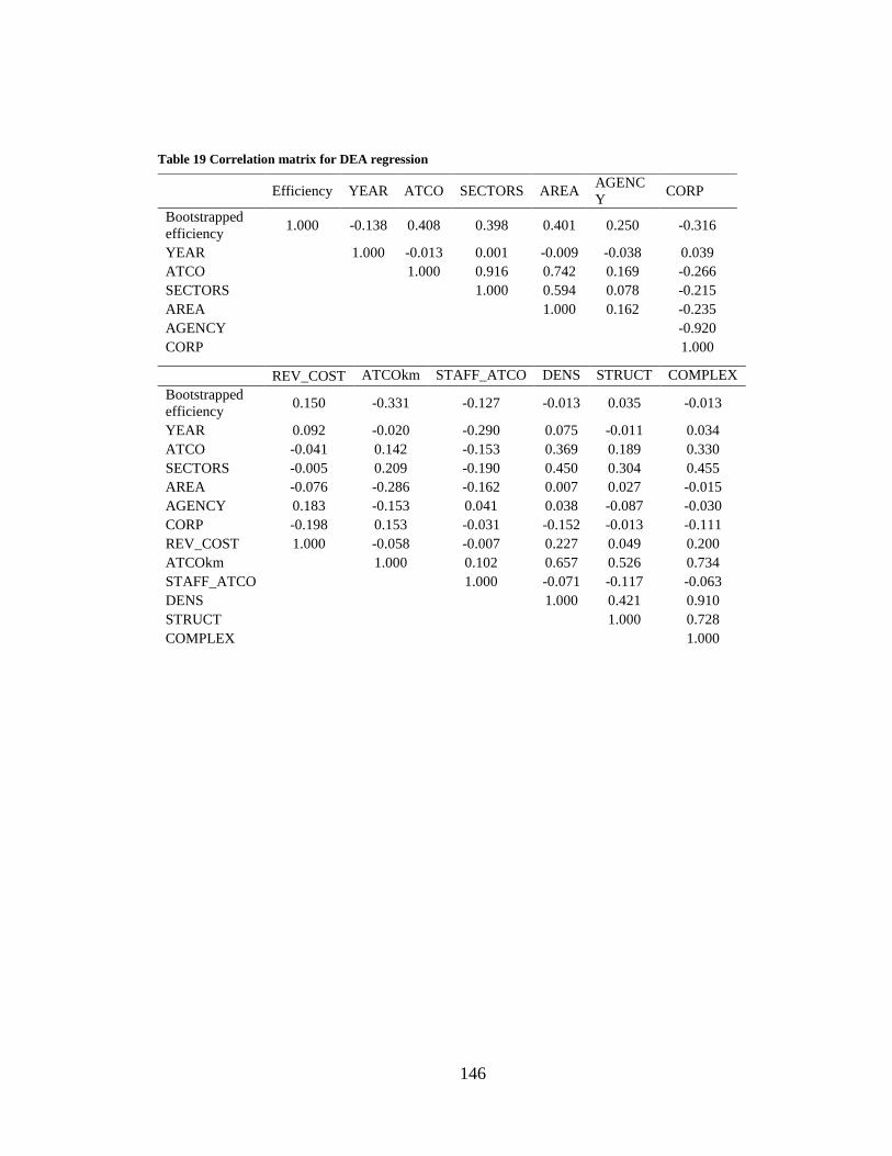
146

Table 19 Correlation matrix for DEA regression

Efficiency YEAR ATCO SECTORS AREA AGENC

Y CORP

Bootstrapped

efficiency 1.000 -0.138 0.408 0.398 0.401 0.250 -0.316

YEAR 1.000 -0.013 0.001 -0.009 -0.038 0.039

ATCO 1.000 0.916 0.742 0.169 -0.266

SECTORS 1.000 0.594 0.078 -0.215

AREA 1.000 0.162 -0.235

AGENCY -0.920

CORP 1.000

REV_COST ATCOkm STAFF_ATCO DENS STRUCT COMPLEX

Bootstrapped

efficiency 0.150 -0.331 -0.127 -0.013 0.035 -0.013

YEAR 0.092 -0.020 -0.290 0.075 -0.011 0.034

ATCO -0.041 0.142 -0.153 0.369 0.189 0.330

SECTORS -0.005 0.209 -0.190 0.450 0.304 0.455

AREA -0.076 -0.286 -0.162 0.007 0.027 -0.015

AGENCY 0.183 -0.153 0.041 0.038 -0.087 -0.030

CORP -0.198 0.153 -0.031 -0.152 -0.013 -0.111

REV_COST 1.000 -0.058 -0.007 0.227 0.049 0.200

ATCOkm 1.000 0.102 0.657 0.526 0.734

STAFF_ATCO 1.000 -0.071 -0.117 -0.063

DENS 1.000 0.421 0.910

STRUCT 1.000 0.728

COMPLEX 1.000

147

8.2. Results Figure 9 provides visual details of the DEA results for the ten years and 37

ANSPs analyzed. The columns not shaded are at least 80% as efficient as the most

efficient providers206

. Table 33 and Figure 15 in Appendix II and III, respectively,

provide more detailed information.

While this 80% benchmark is inevitably arbitrary, the extent of the variability

between the various providers is evident. The ANSPs that have a score of 0.8 or higher in

each of the ten years are, EUROCONTROL, Estonia, Finland, France, and the United

Kingdom. Some others, like Turkey, moved from outside of the benchmark to being

consistently above it, while others like Greece moved the other direction. Fewer

providers met the 80% criteria towards the end of the period than at the beginning.

There are also some oddities in the results – for example, the sudden increases to

the efficiency frontier of Portugal in 2003, Serbia in 2007, and Turkey in 2002. A look at

the input and output data shows that in those years the value for the 1/delays output

variable equals one in those countries, and being one the maximum value for that variable

it makes the ANSP jump to the efficiency frontier. This show the sensitivity of the DEA

analysis to some of the values in the model, and the different specifications tested seem to

indicate that this happens mostly because of this “undesirable output” variable. Given the

206

DEA analysis results can be very sensitive to outliers. To test for this, the model was run removing, in

one case airspace outside of the 10% and 90% percentiles for 2009, and in another traffic controlled over

the same ranges. Additionally, since EUROCONTROL/MUAC is a very different ANSP from the

remaining 36, a model that excluded it was also created. Results for these different models were rather

similar to the basic model and no appreciable differences in results emerge.

148

small number of cases in a dataset of more than 350 observations, this does not appear to

have any significant impact in the results.

Slack analysis (Table 35 in Appendix II) shows that a large number of DMUs,

more than 200, could have achieved the same level of efficiency by reducing the amount

of provision costs that they incur. The same is true for the 1/delays output, with more

than 200 DMUs having slack to increase this output; however, since this is a reciprocal, it

means that if they reduce their amounts of delays, they would be able to maintain the

same level of relative efficiency. For the other two inputs, most DMUs have a slack of

zero, meaning they are operating at their optimal level. Scale efficiency estimates show

that all but 11 DMUs are operating below optimal scale level, but considering the ones

that operate 90% or above of optimal level, there are 107 DMUs (out of 354, 30%) in that

situation.

In terms of allocative efficiency (Table 34 in Appendix II), results show

extremely high average levels, with an average of almost 96% allocative efficiency. This

could either mean that DMUs are using their resources in a very optimized way for their

level of technical efficiency, or, more likely, it might simply be a result of the

specification used.

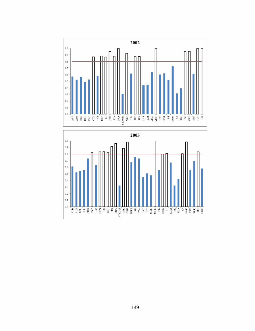
149

150

151

152

153

Figure 9 DEA efficiency results for each year

Key: Albania (ALB), Armenia (ARM), Austria (AUS), Belgium (BEL), Bulgaria

(BUL), Croatia (CRO) Cyprus (CYP), Czech Republic (CZ), Denmark (DEN),

EUROCONTROL (EC), Estonia (EST), Finland (FIN), France (FRA), Republic of

Macedonia (FYROM), Germany (GER), Greece (GRE), Hungary (HUN), Ireland

(IRE), Italy (ITA), Latvia (LAT), Lithuania (LIT), Malta (MAL), Moldova (MOL),

Netherlands (NL), Norway (NOR), Poland (POL), Portugal (PT), Romania (ROM),

Serbia (SEB), Slovakia (SK), Slovenia (SLO), Spain (SP), Sweden (SWE),

Switzerland (SWI), Turkey (TUR), United Kingdom (UK), and Ukraine (UKR).

154

Table 10 presents the results for the four basic models for the regression analysis.

Table 37 through Table 40 in Appendix IV present some additional models that were

tested, which included dummy variables for year and ANSP and traffic complexity

variables.

155

Table 20 DEA bootstrap regression results

Variable

Model

1a

1b

2a

2b

(intercept) 20.27***

(3.953)

20.31***

(3.960)

20.21***

(3.939)

20.24***

(3.942)

YEAR -9.797e-3***

(-3.836)

-9.796-e3***

(-3.835)

-9.772e-3***

(-3.825)

-9.771e-3***

(-3.822)

AGENCY 4.579e-2**

(2.473)

5.507e-3

(0.115)

5.198e-2**

(2.905)

2.150e-2

(0.462)

CORP - -4.235e-2

(-0.913) -

-3.259e-2

(-0.710)

AREA -3.716e-5

(-1.197)

-3.854e-5

(-1.239) - -

SECTORS 2.149e-3**

(2.954)

1.943e-3**

(2.550)

2.977e-3***

(10.476)

2.891e-3***

(9.341)

ATCO 6.006e-5

(1.488)

6.531e-5

(1.601) - -

ATCOkm -5.524e-2***

(-8.040)

-5.463e-2***

(-7.911)

-5.108e-2***

(-9.085)

-5.024e-2***

(-8.898)

STAFF_ATCO -5.938e-3

(-1.236)

-6.333e-3

(-1.312)

-5.513e-3

(-1.149)

-5.787e-3

(-1.201)

REV_COST 8.030e-2**

(2.849)

7.840e-2**

(2.774)

7.927e-2**

(2.851)

7.747e-2**

(2.773)

Adjusted R-squared 0.3858 0.3855 0.3852 0.3844

Variable Model

3a

3b

4a

4b

(intercept) 15.67**

(2.901)

15.64**

(2.905)

20.62***

(3.961)

20.63***

(3.976)

YEAR -7.532e-3**

(-2.798)

-7.469e-3**

(-2.783)

-9.983e-3***

(-3.851)

-9.946e-3***

(-3.848)

AGENCY 7.817e-2***

(4.040)

-9.319e-3

(-0.182)

3.703e-2**

(2.008)

-3.738e-2

(-0.822)

CORP - -9.189e-2*

(-1.843) -

-8.017e-2*

(-1.789)

AREA 8.428e-5***

(3.765)

8.403e-5***

(3.767) - -

SECTORS 1.630e-3***

(4.407)

1.416e-3***

(3.663) - -

ATCO - - 1.245e-4***

(9.813)

1.172e-4***

(8.819)

ATCOkm - - -4.688-2***

(-8.330)

-4.597e-2***

(-8.160)

STAFF_ATCO - - -8.037e-3*

(-1.665)

-8.410e-3*

(-1.746)

REV_COST - - 9.517e-2***

(3.364)

8.987e-2**

(3.169)

Adjusted R-squared 0.2453 0.2504 0.3666 0.3706

Notes ***significant at 0.001; ** significant at 0.05; *significant at 0.1; t-values in parentheses.

Positive signs in the coefficients indicate that the variable is associated with larger levels of efficiency.

156

The results are modest in terms of the overall fit to the data, but the individual

coefficients offer some insight as to the influence of the physical and institutional

environments in which the ANSPs function.

The negative time variable indicates that efficiency has tended to fall over the

period, although given trade-cycle effects on air transportation demand in general, this

should be taken at least in part as a reflection of the generic difficulties for ANSPs to

adjust their capacity and input mix in line with shifting demand patterns. The analysis

with yearly dummy variables shows high levels of significance for the last few years of

the dataset, perhaps a result of the financial crisis of the late 2000’s and subsequent

decline in traffic, leaving ANSPs to have to adjust to falling revenue. This somewhat

contrasts to the general finding by EUROCONTROL in their annual reports, which

shows increases in financial and economic cost-effectiveness, but their analysis is based

on “cost per flight-hour”, a somewhat different measure of efficiency.

The positive sign and consistently high level of significance of the variables

reflecting the numbers of sectors an ANSP handles suggests that there are economies of

some form present although what type of economies are present it is not possible to say.

A similar strong link between the geographic areas for which a provider is responsible is

found, but again, whether this is the result of less congestion or some scale effect in

handling traffic it is impossible to discern207

. The ratio of overall staff employed by an

ANSP to the ATCos employed has a negative coefficient, suggesting that more “front-

line” labor relative to support staff increases the technical efficiency of systems.

207

However, Helios Economics and Policy Services (2006b) suggest that this is due to the presence of

economies of scale.

157

The inclusion of the traffic complexity variables (Table 39 and Table 40 in

Appendix IV) seems to indicate that ANSPs that have to deal with these higher levels of

complexity have higher levels of relative efficiency. This could be a result of the

“incentive” that the presence of this complexity creates, leading ANSPs to become more

efficient in order to be able to deal with this increased complexity.

The nature of the ownership effect, embodied in the AGENCY and CORP

variables, runs counter to much of the work that has been done in other sectors of air

transportation. The findings suggest that ANSPs that are closely linked to the

government, basically direct agents of it, are relatively more efficient than those that have

been corporatized or are public/private partnerships. This is a robust finding across all of

the specifications explored. There may be a number of reasons for this.

While the corporatized entities are more remote from government than those

falling into the “agency” grouping, they are subject to what amount to rate-of-return

regulation – a de facto zero return. This has dangers associated with the “Averch-Johnson

effect” (Averch & Johnson, 1962). This comes about because rate-of-return regulation

creates a strong incentive for companies to over-invest and have a sub-optimally high

capital to labor ratio208

. While this is a problem normally seen as affecting rate-of-return

regulated, profit driven companies, the managerial motivation for efficiency in a non-

profit organization should be identical if they are seeking a constrained internal welfare

maximization. It may also be that that those that have been corporatized were initially the

208

This is often embodied in the notion of ‘gold-plating’ whereby airports’ management provides

excessively high-quality services within a zero profit framework. It can also be seen in a different context

in the form of X-inefficiency whereby the rate-of-return controls allow any cost increases to be passed on

to users thus reducing the incentive for management to minimize costs. This problem can be compounded if

the ANSP has control over information flows about costs.

158

least efficient initially and, because of indivisibilities and the retention of legal

requirements, are taking time to catch up209

– in order to test if this is the case or not, a

longer time series would be needed, as the one available only starts when most ANSPs

had been commercialized already. Put more simply, there remain serious disequilibria in

the markets for ANSs with the corporatized entities still adjusting to their new

situation210

.

8.3. Spatial Autocorrelation Issues211 A possible explanation for the results above is that there may be issues of spatial

autocorrelation whereby the efficiency of one ANSP provider is affected by the

inefficiencies of those around it. Unlike airlines and airports that involve limited vertical

integration with other airlines or airports, one ANSP is often a complementary good with

another, and their efficiencies are thus interdependent. This complementarity is the very

raison d’etre of the Single Sky European initiative.

While the FABs and other SES initiatives do not take place, the system still lives

with a great level of fragmentation. To assess the impact of that fragmentation in the

efficiency of each individual system and its dependence on the spatial distribution of

other systems around it, this section will utilize spatial autocorrelation statistics to study

209

Shocks to the system can also affect efficiency in the short term. The terrorist attacks on New York and

Washington of September 11, 2011, the SARS pandemics, and others, affected air traffic volumes and

some ANSPs were probably in a better position to withstand these shocks better than others. NATS for

example had only just become a public/private enterprise. 210

It may also be that there are endogeneity in play that are not captured in the model, and would be

difficulty to capture for the short time period covered. In particular, the revenues/costs ratio and

staff/ATCos may be endogenous if corporatization or privatization increase the ability to recover costs or

improve labor efficiency; in other words they are collinear with whether the organizational structure is a

government department or a corporation. 211

A previous version of the work presented in this section has been published as Button, K., & Neiva, R.

(2013), Spatial Autocorrelation in the European Air Navigation System, Applied Economic Letters, 20 (15),

1431-1434.

159

that level of spatial dependence of nearby systems212

. As the first law of geography states

(Tobler, 1970, p. 236), “Everything is related to everything else, but near things are more

related than distant things”. The use of spatial autocorrelation is a formal way to measure

that degree of interdependence. From a statistical perspective, autocorrelation exists when

errors in a statistical model are not independent – a basic premise that models must fulfill

in order to be used for hypotheses testing. An ideal model would explain all the variance

and leave residuals that are truly independent. In the presence of autocorrelation, the

chances of having a Type I error increase, resulting in a “false positive” where the null

hypothesis is incorrectly rejected, and a supposed effect is determined to exist where it

does not do so. Although this problem of autocorrelation is mostly analyzed in terms of

time dependency of observations, spatial dependency of observations can also be an issue

when analyzing data where spatial distribution is important (Odland, 1988; Ward &

Gleditsch, 2008).

Two different measures of spatial autocorrelation are tested: the distance between

each pair of countries and whether each pair of countries are “neighbors” or not, i.e., if

their respective airspace share a border. In the context of the SES, the latter assumes a

particular importance, as the handing-out of traffic between countries has been identified

has a source of inefficiencies and the SES aims to tackle that issue.

In order to test for the existence of spatial autocorrelation, the estimates for the

relative levels of efficiency were used to estimate the Moran’s I measure of

autocorrelation (Moran, 1950) – Equation 12 .

212

Spatial autocorrelation was estimated using the R software package with the package “APE: analyses of

phylogenetics and evolution in R language”, version 3.0-11 (Paradis, Claude, & Strimme, 2013).

160

Equation 12

∑ ∑ ( )( )

∑ ( )

Where is the weight between observations i and j, in this case either the

spatial distance between the two points213

or a binary variable stipulating whether two

points share an airspace border214

, x is the measure of interest, in this case the relative

levels of efficiency, and is the sum of all .

Values of I range from −1 to 1, indicating perfect dispersion and perfect

correlation, respectively.

The expected value, which tends to zero, of I under the null hypothesis of no

spatial autocorrelation is presented on Equation 13:

Equation 13

( )

When distances are tested, the values of I are great-circle distances215

between the

airports that have the greatest percentage of landings and departures in each respective

country pair216

. Although only crude approximates, and some features of airspace use are

omitted, notably flights from A to B that flyover C and domestic flights that never leave a

213

Or the inverse of that distance, to be more precise. 214

Using different types of weights allows the testing of different hypotheses for spatial organization

(Odland, 1988). 215

Estimated using the tool available at www.gcmap.com. 216

For example, Lisbon airport (LIS) in Portugal and Schiphol airport (AMS) in the Netherlands are

separated by 1848 km.

161

country’s airspace, given that there is no better publicly available data this measure was

chosen, as a second-best approach to estimating these distances.217

When testing for whether two systems share a border or not, the airspace maps for

each system, available in EUROCONTROL Performance Review Commission (2013a)

were used218

. In this case, a weight of one for represents the fact that i and j share a

border and zero if not. One source of potential misestimates in this case is the fact that the

dataset only includes 37 systems. As such, there is no information about the interactions

with countries outside their combined external borders, so any inefficiencies interacting

with these outside countries are not captured. Another problem is that these weights are

the same values to pairs of ANSPs with very short airspace boundaries and pairs with

very long airspace boundaries.

For this analysis the bias-corrected bootstrapped efficiency results for the last year

of the database were used. Figure 10 shows the DEA relative efficiencies for that year.

217

The ideal scenario would be to have data about all domestic and international flights and do a weighted

average of the distances between each country pair. 218

Note that even if countries do not share a land border they can share an airspace border, e.g., France and

the UK.

162

These results are used to compute the two Moran’s I measures of spatial

autocorrelation (Table 21) estimates using distances and shared borders distinctions.

For the first case, the impacts of distance are small, although positive and

significant at the 5 percent level. This indicates that there is indeed an issue of spatial

autocorrelation in the relative levels of efficiency in the European ANSs system when

considered in terms of distances between the biggest airports in each system and that the

efficiency of a national system is spatially correlated to the others systems. When using

the binary weights for shared airspace borders, the results are still positive and

considerably larger, but not significant even at the 10 percent level219

.

219

Due to the specific nature of the MUAC, which only controls upper airspace, the estimates were also run

excluding it, but the exclusion does not significantly affect the results, neither in terms of significance, nor

sign or magnitude of the coefficients.

Figure 10 DEA relative efficiencies for 2011

163

Table 21 Moran’s I spatial autocorrelation measures

Distance Shared Borders

Observed Moran’s I 0.046 0.150

Expected Moran’s I -0.028 -0.028

Standard deviation 0.033 0.112

These results, although not conclusive220

, add to that rationale in support of

having a “Single Sky”221

by suggesting that there is at least some sort of spatial

dependency from an economic efficiency perspective, with each ANSP being impacted in

its level of efficiency by other systems. In essence, no matter how efficient an air traffic

control system is, its interdependency with other systems may lead to drops in its

performance if third parties are less efficient.

8.4. Total Factor Productivity Figure 11 presents the estimation for the average TFP Malmquist indexes for each

year of the dataset. Figure 16 and Table 36 in Appendix III and II, respectively, present

the individual results for each ANSP. In all these figures TFP values are indexed to the

first of the dataset, starting at 100% in that year.

220

From a technical perspective, when in the presence of spatial autocorrelation, a possible solution to the

problem when running regressions is to include dummy variables for each spatial unit in the analysis. This

was done (Table 38 in Appendix IV) but the results are not much conclusive, with most of the ownership,

operational, and physical variables becoming non-significant, with the majority of significant variables

being country dummy variables. 221

There is, on the other hand, the risk that a merger of airspaces will bring the efficiency down to the

lowest common denominator.

164

The average yearly figure shows, more or less, constant behavior across the years,

with the results hovering around the initial 2002 TFP222

. The big exception is 2008,

where there is a steep decline, perhaps a result of the decline in traffic resulting from the

financial crisis, leaving ANSPs with a mostly fixed cost structure while sustaining

decline revenues. TFP starts to improve soon after as ANSPs begin to adjust to the new

paradigm. A similar thing happened in the beginning of the dataset, with a decline from

2002 to 2003, a period that experienced not only the SARS outbreak but also the decline

in traffic that followed the terrorist attacks of September 11th

2001 in the US. It can be

the case that ANSPs were still coping with that decline in traffic in 2001-2003 and then

managed to adjust their cost structure in 2004 and the following years.

222

Just as a crude comparison, Eurostat reports that overall productivity in economy of the 27 countries of

the European Union – all of the current members except Croatia – increased 10% from 2002 to 2011.

Figure 11 DEA total factor productivity Malmquist indexes – yearly averages

165

Analyzing the TFPs for the individual ANSPs, it can be seen that ANSPs suffer

from a wide range of variation in the TFP values across the years223

, with value of TFP

growth in the entire period ranging from -28% to 14%, but with high levels of variation

in the middle of the time period, with peaks of -32% and +56%. No ANSP is able, for

example, to sustain continued growth in its TFP levels. This can be a result of the

volatility of the market in which ANSPs operate, with variations in traffic that are

unpredictable and subjected to exogenous conditions in the overall economy, and a cost

structure, compounded with full cost recovery requirements, that cannot adjust easily,

leaving ANSPs in a difficult position to adapt.

8.5. An Analysis of the Functional Airspace Blocks224 This section will do an analysis of the FABS by performing a “simulation” on

how would they compare to each if they were operational during the period of the dataset.

This was done by using all the data is reported for individual ANSPs for the

period from 2002 through 2011, and then aggregating it225

at the FAB level to simulate

the operation of the European airspace under that paradigm226

. This is naturally a very

crude approximation of what a FAB will eventually constitute, as it is expected, for

example, that the number and boundaries of en-route sectors will be adjusted to operate

in a more rational manner, thus leading to consolidation of facilities and adjustments on

223

This behavior was also found in the older EUROCONTROL TFP study (EUROCONTROL

Performance Review Commission, 2005b). 224

A previous version of the work presented in this section has been published as Button, K., & Neiva, R.

(2013), Single European Sky and the Functional Airspace Blocks: Will They Improve Economic

Efficiency?, Journal of Air Transport and Management, 33, 77-80 225

Except for Luxembourg – which upper space is controlled by the MUAC – and Bosnia and

Herzegovina, all the countries that constitute the nine FABs are included in this dataset. 226

A similar exercise was done by the latest ACE report, where the financial and economic KPIs were

estimated at the FAB level, and it was found that the level of dispersion of results was much lower

compared to when doing the individual ANSP analysis was conducted.

166

personnel levels. Given the data that is available at the moment, it allows for a

preliminary analysis on how the future FABs stand against each other in terms of

economic efficiency.

This exercise was done using the same variable returns to scale DEA specification

as in the individual ANSP analysis as well as the same variables as inputs and outputs.

Also like in the case of the individual ANSP analysis, the values of relative efficiency for

the FABs were bootstrapped to allow for statistical hypothesis testing using ordinary least

squares regression. The independent variables used were also the same as before, with the

exception of the ownership variables (AGENCY/CORP), which do not make sense to

include in this aggregate analysis. The same four basic models were run.

Table 22 presents some basic information about the statistics used in this analysis,

and Figure 12 the efficiency results in graphical form for the nine FABs in the ten years

of the dataset227

.

227

Table 41in Appendix V presents the detailed values.

167

Table 22 Basic statistics for the variables included in the FAB DEA analysis.

Costs (€) Provision

Costs (€) Revenues (€) Revenues/Costs

Flight Hours

(‘000s)

Mean 835.6 736.2 831.7 1.0 1356.5

Minimum 110.0 92.0 130.0 0.8 286.0

Maximum 3249.0 2796.0 3362.0 1.2 4942.0

Standard

Deviation 847.1 724.2 866.9 0.1 1246.1

N 86 86 86 86 86

Airport

Movements

(‘000s)

Delays

(‘000s

minutes)

ATCO Staff

Mean 1593.9 1751.1 1624 5024

Minimum 120.0 0.0 409 1413

Maximum 5447.0 15373.0 5811 17873

Standard

Deviation 1477.3 2317.0 1428.6 4695.0

N 86 86 86 86

Airport

Movements

(‘000s)

ATCOkm AREA

(‘000s km2)

SECTORS

Mean 3.2 1.4 1186.3 68.0

Minimum 2.1 0.6 400.0 10.0

Maximum 4.4 3.2 2855.0 262.0

Standard

Deviation 0.7 0.7 786.2 67.8

N 86 86 86 86

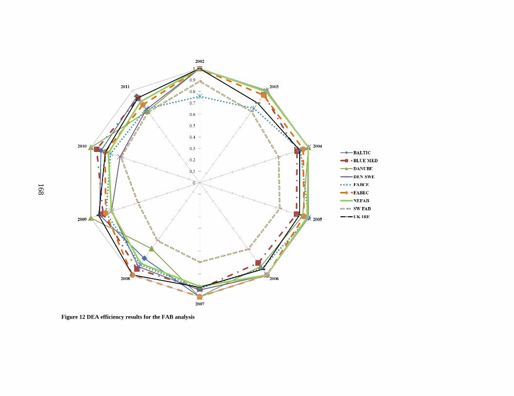
Figure 12 DEA efficiency results for the FAB analysis

168

169

Although at first glance it seems that the FAB aggregation would greatly improve

efficiency, one must keep in mind that since DEA only estimates relative levels of

efficiency, it cannot be concluded that these results are evidence that the creation of the

FABs will lead to system-wide increases in efficiency. Indeed, it is quite possible that the

system could lead to efficiency being pulled down by the least efficient ANSPs.

What can be determined by the figure is that with the exception of the Southwest

FAB (Portugal and Spain), all other blocks tend to consistently stay above the 80%

threshold or be very close to it. The Southwest FAB is the one that drops below 70%.

Of the “established blocks”, UK-Ireland and Danish-Swedish, the former stayed

above the 80% threshold for the entire period, and the latter for all but the last two years

(75% in 2010 and 79% in 2011). As expected, since different systems are being

combined and all the ANSPs are being average into nine blocks, the levels of efficiency

fluctuate much less than in the individual ANSP analysis228

. In one sense, by combining

ANSP’s into FABS, there is some evidence that these combinations would at least be

consistent. Over time, one would expect some fluctuations in relative efficiency, but in

fact the data remains quite stable for most FABs, except for the case of the Danube FAB,

which has two big drops in 2008 and 2011 – a result that seems to be a result of a

considerable increase in the amount of delays reported by the ANSPs that constitute this

FAB for those two years in particular when compared to the other years in the dataset229

.

One explanation for this could be the time it takes for ANSPs to change their structures,

228

A result consistent with the findings of EUROCONTROL in their estimates of the financial and

economic KPIs. 229

Once again, this result shows the sensitivity of DEA in terms of the variations in the values of outputs.

170

but this is essentially speculation. If this were so, it could be a cyclical effect, with

inflexible equipment needing periodic upgrading230

, or it could be shorter term as a

function having to spread fixed costs over fluctuating demand patterns.

Like in the case of individual ANSP analysis, allocative efficiency levels (Table

42 in Appendix V) are also quite high. In fact, they are even higher than in the individual

analysis, with an average of more than 98%. Once again, this might be the result of

optimal use of resources, or a byproduct of the model specification used. Slack analysis

(Table 43 in Appendix V) shows that most of the variables are being used/produced at

optimal levels, with the exception of airport movements for which some FABs present

some rather large numbers. This suggests that they could improve their performance;

however, airport movements control is mostly a localized issue. As such, efficiency gains

from the merging of ANSP operations will be less likely at this level. In terms of scale

efficiency, out of the 86 DMUs, 15 operate in the optimum scale level, while 38 (44%)

operate at levels of 90% or higher of optimum scale, suggesting that the FAB aggregation

leads to a more optimal scale, when compared to the individual ANSPs.

To better understand factors that may be affecting the cross-sectional pattern of

the programming results and their changes over time, the bias-corrected bootstrapped

efficiencies obtained from the DEA efficiencies were regressed on a number of

parameters using the same four models as in the individual ANSP analysis.

Table 23 presents the correlation matrix of bilateral relationships for the variables

included in the model and Table 24 the regression results.

230

Given each FAB represents a collection group of ANSPs it is unlikely that all would be upgrading their

systems simultaneous.

171

Table 23 Correlation matrix for FAB DEA regression

The correlation matrix show a flagrant case of correlation between the number of

ATCos and the number of en-route sectors, with an almost perfect correlation, while

other pairs of independent variables have for the most part low levels of correlation.

Efficiency YEAR ATCOs SECTORS AREA

Efficiency 1.000 -0.340 -0.051 0.015 -0.455

YEAR 1.000 -0.003 -0.027 -0.031

ATCOs 1.000 0.979 0.598

SECTORS 1.000 0.503

AREA 1.000

REV_COST ATCOkm STAFF_ATCO

Efficiency 0.341 0.181 0.293

YEAR 0.139 0.000 0.031

ATCOs 0.099 0.650 -0.128

SECTORS 0.179 0.686 -0.062

AREA -0.229 -0.110 -0.636

REV_COST 1.000 0.259 0.356

ATCOkm 1.000 0.508

STAFF_ATCO 1.000

172

Table 24 FAB DEA regression results

Variable Model

1

2

3

4

(intercept) 27.27***

(5.576)

25.04***

(4.291)

22.71***

(4.310)

24.70***

(4.260)

YEAR -1.321e-2***

(-5.405)

-1.2252e-2***

(-4.204)

-1.086e-2***

(-4.136)

-1.207e-2***

(-4.169)

AREA -1.301e-4***

(-6.232) -

-6.947e-5***

(-6.393)

-

SECTORS -9.127e-4

(-1.522)

-1.959e-4

(-0.871)

4.121e-4**

(3.269)

-

ATCO 1.053e-4**

(3.035) - -

-1.301e-5

(-1.236)

ATCOkm -7.796e-2**

(-3.025)

1.7834e-2

(0.731) -

2.509e-2

(1.035)

STAFF_ATCO -4.461e-3

(-0.265)

1.2457e-2

(0.629) -

6.490e-3

(0.319)

REV_COST 2.742e-1**

(2.936)

3.6526e-1**

(3.367) -

3.593e-1**

(3.406)

Adjusted R-squared 0.5052 0.2636 0.3883 0.2705

Notes ***significant at 0.001; ** significant at 0.05; *significant at 0.1; t-values in parentheses.

Regression results show that the variables are mostly non-significant, and the

levels of fitness are somewhat low, but a few results stand out, as is the case of the

greater number of en-route sectors in Model 3 being associated with higher levels of

relative efficiency, while both the area of airspace controlled in Models 1 and 3 and the

number of ATCos per unit of area in Model 1 are associated with lower levels of relative

efficiency.

These results would suggest that there may be some optimum level of sectors or

airspace that would maximize efficiency231

. The efforts of forming FABs can be

considered as a first approximation at achieving this. The difficulty, however, is that this

231

Analysis with the inclusion of dummy variables for country and year (Table 44and Table 45 in

Appendix IV) show some different results, with coefficients for the different variables having more

variation in the direction.

173

information tells little about the parameters of an optimal situation. The FABs are

combinations of national airspaces, each of which may well contain areas of efficient

ANS provision and some inefficient areas. They are in no way axiomatically optimal

spaces; they are just politically determined “market areas”. Combining them may

increase efficiency over some parts of airspace but equally reduce it over other areas.

From a dynamic, incentive perspective, while the data analysis is insightful in

terms of tracking previous patterns of efficiency, it offers little insight into whether the

gradualist approach towards a SES via way stations of FABs is either optimal or likely to

succeed. While a “big bang” approach limits the opportunities for coalitions to capture à

la Stigler (1971) any reform process during transition, gradualism provides more

opening. In the FAB case, the incentives to collaborate are not many, and many national

interests can oppose any level of collaboration; particularly, for less efficient blocks there

are limited incentives to move forward and that can either limit the full benefits that

could come from an ultimately completely integrated European ANS, or de facto demand

“bribes” in the form of restructuring payments to move forward. By combining in

groupings of similar FABs, the bargaining position of any individual ANSPs increases.

The outcome of this is much less of a technical economic matter and much more to do

with political economy.

The analysis here provides insights into the nature of the FABs by looking at their

relative efficiencies over time and some factors that may explain differences. Yet, it

describes little more than background to a largely political process, but it does highlight

some of the quantitative considerations that need to be considered.

174

8.6. Difference-in-Differences From the 37 ANSPs in the dataset only four of them changes ownership status

during the 2002-2010 period:

Macedonia in 2010;

Poland in 2007;

Sweden in 2010;

Slovenia in 2004.

Except for Poland, in which the previously commercialized ANSP that used to be

part of the company that also operated the country’s airports was spun off into a

government agency, the three other ANSPs were commercialized during this period.

Considering that the dataset included data from 2002 to 2011232

, it can be seen that the

timespan before and after the changes is not extensive, perhaps not leaving enough time

for the “treatment” to take effect. Additionally, only four ANSPs remained non-

commercialized for the entire 2002-2011 period, leaving a very small number of

observations to include in the comparisons with the three ANSPs that were

commercialized.

With these caveats in mind, the D-i-D approach was used to test if there were any

effects in the relative efficiency due to the chances in ownership233

. The Polish ANSP

was tested against the 29 ANSPs that had been commercialized before the timespan of

the dataset, and the other three were compared to the four ANSPs that remain non-

commercialized. Table 25 shows the estimate results.

232

Additionally, data for Poland is only available since 2005. 233

Difference-in-differences was estimated using the R software package with the package “wfe: Weighted

Linear Fixed Effects Regression Models for Causal Inference”, version 1.2 (Kim & Imai, 2013).

175

Table 25 Differences-in-differences estimate

Country

Poland Slovenia Sweden FYROM

D-i-D estimate -0.0382* 0.1704** -0.1648** 0.0154

t value -2.055 3.726 -10.215 0.952

Notes **significant at 0.001; * significant at 0.05

Estimates for Macedonia are not significant, not even at the 10% level. For the

other three estimates are significant, but rather inconclusive. The “treatment” applied to

Poland seems to have resulted in a decrease in efficiency compared to what would have

happened if it remained commercialized, but in the case of Slovenia and Sweden, both

commercialized during this period, results have different directions. For Slovenia,

commercialization seems to have resulted in increased efficiency, and for Sweden, the

opposite happened.

The application of the D-i-D approach does not help to address the issue of

identification for the impacts of commercialization in the provision of air navigation

services. Several reasons can possible explain these results. One is the short period of

time considered for the estimate, as all countries change ownership almost at the

beginning of the period or at the end, not allowing the D-i-D specification to “capture”

the true trends before and/or after the treatment and leading to wrong estimates of the

treatment effect. Another possibility is that there might be a number of exogenous

variables not captured in the model that are affecting the different ANSPs in different

ways. Since the D-i-D approach assumes that trends are the same for both the control and

treatment groups, it might be the case that the models used are simply too simplistic to do

this analysis.

176

8.7. Discussion The structure and governance of ANSPs has been changing over time. They are

provided under a number of different regulatory regimes, within a variety of ownership

structures, and subject to a number of external conditions. The results of applying

programmatic techniques to look at the diversity of systems that exist within Europe

indicate a wide dispersion in the relative levels of efficiency that is found and that

patterns tends to change over time. Some systems have maintained a high level of relative

efficiency; others have improved their relative positions, but a number consistently tend

to fall behind. Some of the explanation for this can be found in the operating environment

under which ANSPs exist, such as the airspace or number of sectors that they cover, but

additional factors within ANSP’s control, such as the ratio of ATCos to overall staff are

also connected to efficiency. In terms of institutional structure there is no evidence from

the data that movement to less government control results in relatively more efficient

ANSPs, indeed the opposite finding emerges. However, one should not jump to the

conclusion that commercialization efforts are worthless, as there might be other

underlying causes in particular characteristics of the systems that could be affecting the

results. Some were tested in this analysis, including operational and physical

characteristics and the presence of spatial autocorrelation, which estimates indicate that

exists at least at some extent, but it might be that some were left out. Causality tests in the

form of differences-in-differences estimates do not help to shed a light in this regard, as

their results are rather inconclusive.

177

CHAPTER 9 – STOCHASTIC FRONTIER ANALYSIS

9.1. Model Specification

The SFA model will make use of a production function to model ANSs

production in Europe, using both a Cobb-Douglas and a translog specification.234

A general specification of a production function can be written as Equation 14,

Equation 14

( ) ( )

Where the output is a result of inputs x, a number of explanatory variables X,

unknown parameters , and an error term e that accounts for unobserved variables and/or

inefficiencies.

SFA also can be used with cost functions, but these require prices for the inputs,

which are not directly available. As such, it was decided to just use a production

function.235

This production function will make use of the accounting data presented in the

ACE reports for the three inputs, and the single output will be the composite flight-hours

reported for each ANSP236

.

234

The models were estimated using the R software package with the package “frontier: Stochastic Frontier

Analysis”, version 1.1-0 (Coelli & Henningsen, 2013). 235

For an application of a Cobb-Douglas cost function in a SFA analysis for the European ANSs system

and how the issue of lack of input prices was tackled see Competition Economists Group (2011).

Estimations with a SFA model similar to the one used in this dissertation found an inefficiency of 57% for

the entire system, but the effects of ownership were not tested. For another attempt at modeling a cost

function for the industry, this time using a translog parameterization, see Button & Neiva (2013).

178

The use of a single output, instead of the two outputs used in the DEA

specification, is due to the fact the specification and estimation of a production function

with multiple outputs involves an additional layer of complexity. Since

EUROCONTROL provides this composite output variable for each ANSP, it was decided

to go with the simpler case of a single output.

In terms of inputs, the following will be used:

Staff costs, including both air traffic controllers and other staff;

Other provision costs, which include capital and depreciation costs, a

generic “non-staff operating costs” and “exceptional items”;

Non-provision costs, ranging from aeronautical meteorological costs,

EUROCONTROL costs, payments for regulatory and supervisory

services, and payments to governmental authorities (e.g. for the use of

government-owned assets).

These costs could have been divided in a greater number of categories, as they are

reported in 12 different subcategories, but using more categories would have complicated

the specification and estimation of the function and possibly lead to some models that

would have been undetermined from a computational perspective. It was decided to use a

simpler specification that separate operating costs in both staff and non-staff costs (for

example in 2011 these represented on average 63% and 37% of operating costs,

respectively) as well as another category for non-operating costs, which represent a small

percentage of total costs for most of the ANSPs.

236

As a reminder, composite flight-hours, are a composite variable estimated by EUROCONTROL that

combines both airport movements and flight-hours controlled.

179

The use of accounting data in production functions is a contentious subject in the

literature; the main drawback being that it is argued that the use of accounting data will

lead to parameter estimation that does not represent the underlying technological

characteristics of the industry. Thus, post-estimate micro-economic analysis, like for

example in terms of the elasticities of inputs, will not be scientifically sound (Bogetoft &

Otto, 2011). The traditional neo-classical production function makes use of figures for

labor and capital that represent, for example, total man-hours and the value of assets,

respectively. However, the data available for this industry does not suit itself well for

this. For instance, total man-hours worked are reported only for ATCos, not for other

employees of the ANSP237

. Since the main goal of this analysis is to assess the impact of

ownership on efficiency results and not a more detailed micro-economic analysis of the

production of air navigation services in Europe, and reported accounting data is mostly

consistent throughout the data, it will be used as inputs in the production function.

The Cobb-Douglas and translog specifications are presented, in logarithmic form,

in Equation 15 and Equation 16, respectively:

Equation 15

( ) ( ) ( ) ( )

Equation 16

( ) ( ) ( ) ( )

( )

( )

( )

( ) ( ) ( ) ( ) ( ) ( ) Where,

237

See EUROCONTROL Performance Review Commission (2011) for a possible way to address these

data issues.

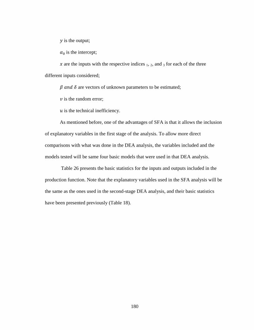
180

is the output;

is the intercept;

are the inputs with the respective indices 1, 2, and 3 for each of the three

different inputs considered;

are vectors of unknown parameters to be estimated;

is the random error;

is the technical inefficiency.

As mentioned before, one of the advantages of SFA is that it allows the inclusion

of explanatory variables in the first stage of the analysis. To allow more direct

comparisons with what was done in the DEA analysis, the variables included and the

models tested will be same four basic models that were used in that DEA analysis.

Table 26 presents the basic statistics for the inputs and outputs included in the

production function. Note that the explanatory variables used in the SFA analysis will be

the same as the ones used in the second-stage DEA analysis, and their basic statistics

have been presented previously (Table 18).

181

Table 26 Basic statistics for the variables included in the SFA analysis.

9.2. Results Table 27 and Table 28 presents some main results for the four models

238 under the

Cobb-Douglas and translog specifications, respectively. In the appendices VIII, IX, and

X, the complete results are presented, included the full regressions (Table 50 and Table

51), and the technical inefficiencies in table (Table 46 to Table 49) and figure format

(Figure 19 and Figure 20).

238

A number of different models besides the four basic models were also tested, including the ones that

were tested in the DEA analysis. Results follow the same trends reported in these four basic models, so it

was decided to just present these.

Staff costs

(€ million)

Other Provision

Costs

(€ million)

Non-provision

costs (€ million)

Composite

Flight Hours

(‘000s)

Mean 118.5 36.8 14.3 476.1

Minimum 2.9 1.1 0.0 7.0

Maximum 777.9 221.3 112.0 2800.0

Standard

Deviation 161.4 46.6 20.2 616.9

N 354 354 354 354

182

Table 27 SFA main regression results for Cobb-Douglas specification

Notes ***significant at 0.001; ** significant at 0.05; *significant at 0.1; z-values in parentheses.

Positive signs in the coefficients indicate that the variable is associated with larger levels of inefficiency.

Table 28 SFA main regression results for translog specification

Model

1 2 3 4

AGENCY -0.4476**

(-3.136)

-0.4446***

(-3.441)

-0.5875

(-0.738)

-0.4409**

(-3.264)

Mean

inneficiency 57.2% 56.4% 64.6% 56.3%

Mean

efficiency 42.8% 43.6% 35.4% 43.8%

0.2649 0.2634 0.6099 0.2839

0.0049 0.0036 0.0230 0.0029

λ2

54.5020 73.6267 26.5634 97.1366

Variance due

to inefficiency 98.2% 98.7% 96.4% 99.0%

Variance due

to random

variation

1.8% 1.3% 3.6% 1.0%

Log likelihood -123.7455 -127.6297 -184.4589 -136.9606

Notes ***significant at 0.001; ** significant at 0.05; *significant at 0.1; z-values in parentheses.

Positive signs in the coefficients indicate that the variable is associated with larger levels of inefficiency.

Model

1 2 3 4

AGENCY 0.3945***

(4.215)

-0.2933

(-0.304)

-0.2104*

(-1.756)

-0.3701***

(-3.387)

Mean

inneficiency 77.5% 59.8% 57.0% 54.6%

Mean

efficiency 22.5% 40.2% 43.0% 45.5%

0.0138 0.4429 0.2509 0.2537

0.0987 0.0297 0.0298 0.0059

λ2 0.1402 14.9039 8.4313 42.8957

Variance due

to

inefficiency

12.3% 93.7% 89.4% 97.7%

Variance due

to random

variation

87.7% 6.3% 10.6% 2.3%

Log

likelihood -104.3407 -173.1192 -163.5451 -151.6983

183

In order to test if using the translog specification instead of the simpler Cobb-

Douglas one239

would increase the significance of the results a simple likelihood ratio test

was conducted (Table 29).

Table 29 SFA specifications likelihood ratio tests

Model

1 2 3 4

χ2

38.81 90.98 41.83 29.48

Probability > χ2 <0.0001 <0.0001 <0.0001 <0.0001

The assumption in these tests would be that the Cobb-Douglas functions were

nested in the associated translog specifications. The results obtained are statistically

significantly and indicate that using the translog specifications result in a statistically

significant improvement in model fit.

In terms of mean inefficiencies, except for Model 1 of the Cobb-Douglas

specification, results are quite consistent, ranging from 55 to 65 percent. The results are

also consistent to what Competition Economists Group (2011) estimated (57%) in their

SFA analysis using a similar SFA specification – albeit with a cost function instead of a

production function. These results suggest that there is a great level of average

inefficiency in the European system.

When comparing individual technical efficiencies obtained from this SFA

analysis to the ones that were obtained using DEA analysis, as expected, efficiencies

obtained using SFA have lower values and more variation between them. On average,

239

It should be remembered that the Cobb-Douglas is a restricted version of the translog specification, or to

put it in another way, the translog function is a generalization of the Cobb-Douglas.

184

Cobb-Douglas efficiencies were 5.5 percentage points lower than DEA efficiencies, and

translog efficiencies 9.1 percentage points.

Table 30 and Figure 13 present some basic comparisons, showing the quartiles of

the estimated technical efficiencies and plotting DEA and translog average efficiencies,

respectively.

Table 30 DEA vs. SFA efficiencies comparison Efficiency

Percentile DEA SFA Cobb-Douglas

(average)

SFA translog

(average)

25% 0.5435 0.4179 0.3921

50% 0.6690 0.6438 0.5780

75% 0.8339 0.8307 0.8041

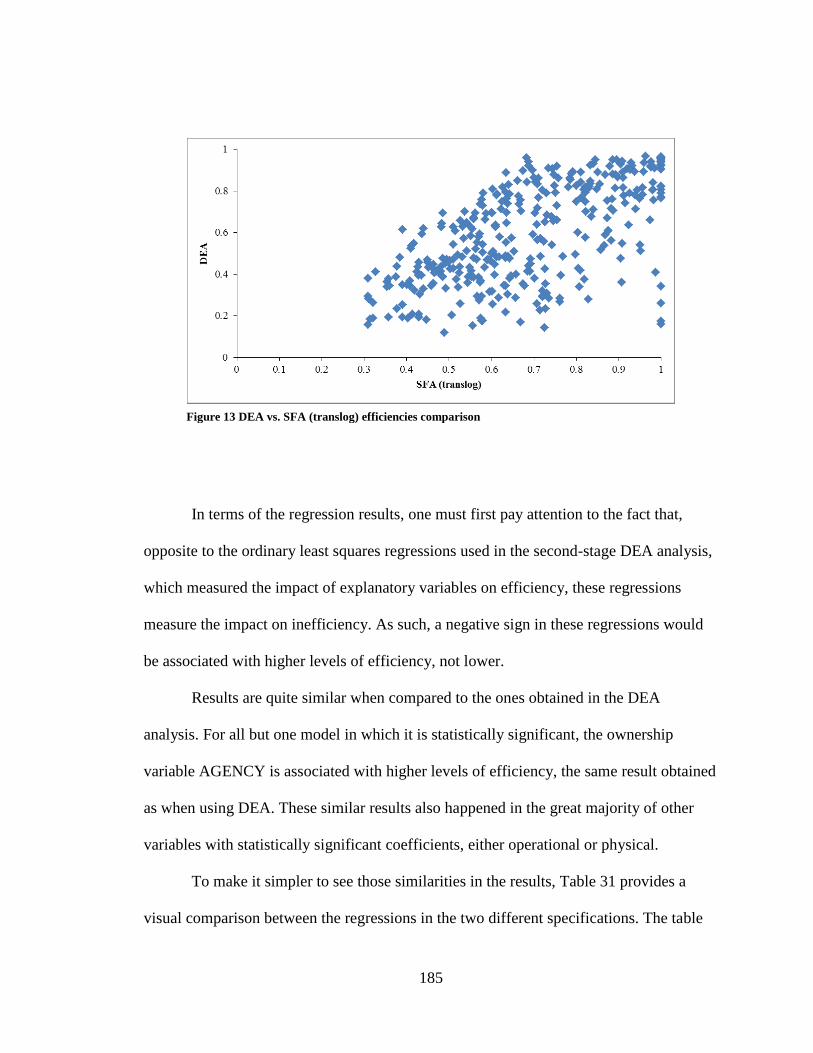
185

In terms of the regression results, one must first pay attention to the fact that,

opposite to the ordinary least squares regressions used in the second-stage DEA analysis,

which measured the impact of explanatory variables on efficiency, these regressions

measure the impact on inefficiency. As such, a negative sign in these regressions would

be associated with higher levels of efficiency, not lower.

Results are quite similar when compared to the ones obtained in the DEA

analysis. For all but one model in which it is statistically significant, the ownership

variable AGENCY is associated with higher levels of efficiency, the same result obtained

as when using DEA. These similar results also happened in the great majority of other

variables with statistically significant coefficients, either operational or physical.

To make it simpler to see those similarities in the results, Table 31 provides a

visual comparison between the regressions in the two different specifications. The table

Figure 13 DEA vs. SFA (translog) efficiencies comparison

186

presents the number of times that a variable was found to have a positive or negative

effect on the efficiency results, with a significance level of at least 10%, or the number of

times it was found to be non-significant. 240

Table 31 DEA vs. SFA explanatory variables comparison

9.3. Discussion The regression results in the SFA analysis have, for the most part, the same

direction of what was obtained using a DEA framework, and this happens not only in the

“major” variable of interest (ownership) but also in most of the operational and physical

variables.

This would suggest that the results are robust across specifications; however,

there are some technical reasons in the SFA specifications that can hinder the scientific

soundness of these results. In all but one of the specifications, the variance due to

inefficiency is the great majority (90% or more) of the variance in the model. This would

suggest that there is no noise in the data and that all deviations from the frontier originate

240

The models compared were the four “main” models of DEA and both SFA specifications.

Variable

Model

DEA SFA

Effect on efficiency Effect on efficiency

Positive Negative Non-

significant Positive Negative

Non-

significant

AGENCY 4 0 0 4 1 2

AREA 2 0 0 2 0 2

SECTORS 4 0 0 4 0 2

ATCO 1 0 1 2 2 0

ATCOkm 0 2 0 1 5 0

STAFF_ATCO 0 1 2 0 5 1

REV_COST 3 0 0 2 0 4

187

almost entirely from inefficiency, indicating that a non-stochastic approach (DEA, for

example) would work best in this case (Coelli et al., 1998)241

. However, it is probably

unrealistic to assume that the dataset does not have any noise in it, and it is probably the

case that the model is biased. A few reasons can potentially be the cause: poor choice

and/or misspecification of the functional form, the real noise term is not normally

distributed, the real inefficiency term does not follow a truncated normal distribution, or

that the noise term and/or the inefficiency term is not independent of the explanatory

variables.

A more detailed analysis would be needed to assess what the causes of these

results were. Some other variations of the model were tested, including the use of more

disaggregated inputs and non-adjusted monetary values; the problem of very high

percentages of variance due to inefficiency persists, suggesting that there are other

underlying problems in the specifications used.

Nonetheless, these results should not be seen as an indication that it is not

possible to model ANSP efficiency using SFA frameworks and that non-stochastic

approaches are the only way to do this, but rather that the specifications that were chosen

do not seem to be the most suited for this specific problem.

241

In fact, the only specification in which the explanatory variable AGENCY does not have the same

direction as in the DEA models is the one (the first Cobb-Douglas model) where the percentage of variance

due to random errors is greater (88% vs. 12%) that the percentage of variance due to inefficiency.

188

CHAPTER 10 – CONCLUSIONS

10.1. Research Findings

As a reminder, the two research questions/hypotheses that were explicitly tested

were:

1. Are “commercialized” ANSPs associated with better economic efficiency

than “public agency” ANSPs?

2. Is the impact of non-policy variables, namely operational and physical

ones, significant in terms of explaining differences in economic efficiency?

A simple answer to these questions would be “no” to the first one, and “yes” to

the second, as results indicate that public agency ANSPs are associated with better

economic efficiency than commercialized ones and that operational and physical

variables are also associated with differences in economic efficiency.

As for the first research question, although results do indicate that public agencies

are indeed associated with better efficiency outcomes, and this is a finding robust across

the different specifications used242

, a number of factors might be playing a role here that

the model is not capturing. These include the fact that all ANSPs, commercialized or not,

are operating in a not-for-profit environment, tantamount to a zero rate-of-return

regulation with the problems, X-inefficiency and Averch-Johnson effect, that it brings. It

242

With the caveat that the SFA specification might have some problems that could potentially undermine

the soundness of its results.

189

might also be the case that the first systems to be commercialized were the ones that were

underperforming, because there are more incentives for a government to do so if this is

the case. This leads to issues of endogeneity, because systems that were commercialized

were not randomly selected to do so. Additionally, although remaining public agencies,

most ANSPs already have at least some features that are associated with commercialized

ANSPs, namely some sort of independence from the government bureaucracy243

, and the

ability to raise their own revenue, be it from charging user fees, or even being able to

access capital markets. This leads to a situation where in some cases the distinction

between commercialized and non-commercialized ANSPs might be a blurry one, and the

de facto and de jure situation might be different.

For the first issue, it would be interesting to analyze how the industry evolves and

its efficiency is affected by Regulation (EC) 1191/2010. This new regulatory scheme will

break the full cost recovery requirement in the ANSs system, and will allow ANSPs to

keep parts of their profits to create buffers against downturns, instead of having to

redistribute them immediately to the airspace users, and then entering the vicious circle of

having to increase charges when traffic falls. This will change the rate-of-return

requirements for the industry, allowing them to react in different ways to the markets

conditions.

For the other point, unfortunately data availability is a problem, and it cannot be

used to prove or disprove the point. Another issue also related to data availability is that

243

On the other hand there are commercialized ANSPs that have great level of dependence from their

governments, which nominate their administration and will sack them easily if the government agenda is

not being implemented.

190

the sample of non-commercialized ANSPs is much smaller compared to the sample of

commercialized ANSPs, which could bring problems, not only in the modeling of the

problem, but also in testing causality links in the commercialization “treatment” – more

on data issues will be discussed in Chapter 10.3 – Research Limitations.

As for the second research question, a number of operational and physical

variables seem to be significantly associated with efficiency outcomes. An increase in

value of the variables related to airspace, numbers of sectors, number of ATCos, and

revenue/costs ratio is associated with higher levels of relative efficiency, while an

increase in the variables related to the number of ATCos per unit of area and in the total

staff/number of ATCos is associated with lower levels of relative efficiency. These

results seem to indicate that there are optimized levels of operation for ANSPs; however,

it is not possible to determine exactly what that level is, but at least they indicate that

systems that operate larger airspaces, more sectors, and are able to recover their costs in a

greater extent, are associated with higher levels of efficiency. It was also found that there

is at least some level of spatial autocorrelation in the European system that is having

impacts at the levels of economic efficiency. All these findings add to previous findings

from other sources that the level of fragmentation in the European ANSs system is having

impacts on the level of efficiency of the system. Additionally, the results from the total

staff/number of ATCos ratio variable seem to indicate that a focus on the “core mission”

of providing ANSs. Thus, having more personnel who control traffic as a total of

employees is associated with higher level of economic efficiency.

191

Besides these two main findings, total factor productivity estimates in the DEA

framework show that the system did not improve, from this perspective, during the period

considered. This is somewhat surprising, as it would be expected that at least some small

level of improvement would be achieved. By analyzing the results, it can also be argued

that this could be a result of the difficulty of the industry in quickly adapting to changing

market conditions, namely declines in traffic resulting from macro-economic factors. The

way charges were imposed onto airspace users during this period might also play a role

here, since it did not create the conditions for ANSPs for structure their operations in the

long-term, making them much more dependent of short-term economic conditions.

10.2. Policy Implications Commercialization has been promoted as a way to improve the efficiency of

ANSPs, and the research in this dissertation aimed to analyze that issue. Results are not

conclusive, although the findings suggest that commercialization is not associated with

higher levels of efficiency. There are a number of other issues that impact the industry

that could be potentially affecting these results. Additionally, results merely indicate that

being non-commercialized is associated with higher levels of economic efficiency during

this relatively short time period of ten years; it does not provide any indication on how

the systems have evolve pre and post-commercialization in order to assess if

commercialization was, in fact, associated with improvements in economic efficiency

that would have not happened otherwise.

The spatial correlation results and the coefficients of the non-policy variables in

the regressions seem to support the rationale behind the efforts of the Single European

192

Sky to reduce fragmentation in the European ANSs system. The same results have been

found before, and in that regard, the dissertation does not greatly contribute to the

literature; it merely confirms previous findings using more up-to-date data.

One issue about commercialization is the issue of equity and access to airspace.

Traditionally, ANSPs followed principles of network pricing, in which charges were set

at the national level. This meant that more remote locations or less used airports, in which

the marginal cost to control a single plane is higher, were being subsidized by areas

where the marginal costs were smaller due to heavier use of the airspace and terminal

facilities. This is still the case in most ANSPs, but some, like the ones in New Zealand

and Australia, have adopted location-specific pricing in which the prices charged are

more directly linked to the costs of providing the service. For example, in Australia, the

price charged in 2013-2014 to a plane that wants to use the control facilities of an airport

varies from AUD$1.94 to AUD$14.21 per metric ton of maximum takeoff weight, a

factor of more than seven (Australian Competition and Consumer Commission, 2011).

The implementation of location-based charging principles was seen as needed due

to issues of equity, and to eliminate, or at least mitigate, cross-subsidies between the

different users of the airspace. Network pricing was also seen a protectionist measure to

make foreign airlines, which normally travel to more populated areas, subsidize more

expensive domestic services within a country. On the other hand, network pricing can

also be seen as promoting access to airspace, as it allows users of remote locations to be

able to afford services that if charged the full price, they would not be able to do so. It

can be also argued that location-based pricing does not take into account the costs of

193

congestion of airspace because even though the marginal cost of controlling an additional

plane in a heavily used area might be smaller, the costs that that additional plane imposes

on the system can potentially be much larger due to the congestion it imposes on other

users of the airspace. This is thus a difficult equilibrium, from wanting to improve equity

in terms of charging principles, to not wanting to decrease equity in terms of access to

airspace (United States Government Accountability Office, 2005).

Another policy issue with commercialization is how to deal with ANSP profits.

Even in the cases where the system is partially (UK) or fully (Canada) privatized, the

regulated parts of the ANSPs are subjected to not-for-profit requirements. In Europe,

until recently, every profit that was gained in the operation had to be redistributed back to

the airspace users. Nevertheless, as it was discussed in Chapter 3.1, this form of rate-of-

return regulation has problems in terms of promoting long-term efficiency improvements.

Although unlikely, it is not unthinkable that a purely for-profit ANSP would be created at

some point, even if it remains to have some sort of pricing regulation. However, this

possibility brings another set of questions in itself, as from a policy standpoint it can be

argued that the use of profits for the own gain of the ANSP or its shareholders instead of

using them to improve social welfare, be it reinvesting in the system or be redistributing

the profits to the airspace users, would not be socially optimum.

Experiences in the airport industry can shed some light on this, as there are cases,

for example many airports in Europe, where airport operators can use profits to reward

shareholders. In contrast, in places like the US federal regulations do not allow revenue

diversion and mandates that revenue must be used for capital and operating costs of the

194

airport itself, the local airport system, or other facilities that are directly related to the air

transportation of passenger or goods, where profits have to be reinvested back into the

system. Seeing how the industry and other stakeholders evolve and behave in Europe

with EC Regulation 1191/2010, which will break full cost recovery requirement in the

ANSs system, will also provide insights into this question.

10.3. Research Limitations

Perhaps the greatest limitation of this study is the timespan of the data considered

in the analysis, which ran from 2002 to 2011. This creates problems for two reasons: due

to the amount of sunk costs that it has, and due to the level of specialization that air

traffic controllers have, the industry is quite slow at adapting, and it might be the case

that ten years, especially ten years that followed a major international event like the

terrorist attacks of September 11th

, 2001, encompassed several health crisis like SARS or

swine flu, and culminated in the greatest economic recession in almost a century244

, is not

a timespan long enough to discern long-term trends and study the evolution of such an

industry. Nevertheless, the timespan, although not ideal, is large enough to at least get a

glimpse of the workings of the industry in terms of economic efficiency.

The other reason is of a more technical nature in what economic analysis is

concerned: with such a timespan, it was not possible to encompass the periods before and

after commercialization for the majority of ANSPs that are commercialized. Even for the

ones in which the timespan studied encompasses changes in ownership – only four out of

244

On the other hand it can be argued that the existence of major disruptive events like these should be

expected, and that these ten years were not atypical in that regard.

195

37 –, the time elapsed before and after the changes is quite small. This creates a serious

issue for identification and causality analysis. This type of analysis is always difficult,

because unlike natural sciences, in economics, it is quite difficult to create control and

treatment groups to study the effects of a given “treatment”. In this particular case, the

“treatment” in question was a policy decision of commercializing an ANSP, and it was

found that ANSPs did not go through commercialization were associated with higher

levels of economic efficiency. These results should be interpreted with care, as other

variables might be influencing the results in ways the models are not capturing. There are

ways to try to deal with this, and this research tried an approach – the difference-in-

differences method – but the results are unclear and do not help much in enlightening the

issue. The lack of data undermines the possibility of further study into this question.

Another limitation of the study is the focus on frontier analysis and potential

problems within that analysis. Although frontier analysis has been gaining prominence in

the literature, other approaches are still useful – namely non-DEA estimations of TFP –

and could improve the results of this study. Within the frontier analysis models used, the

issue of specification of those models can also be considered a limitation. In both DEA

and SFA approaches, it was decided to use an approach that included costs as inputs and

physical variables as outputs, but many more possibilities exist, as it cannot be argued

that the approach that was followed is the more appropriate to answer the research

questions. In the SFA analysis, the choice of a production function over a cost function

was done mainly due to the availability of data, but it would also be interesting to try that

196

approach, especially since the results of this SFA analysis seems to indicate the

specification used is not the most appropriate for the problem at hand.

The institutional treatment of the ANSPs is also a limitation of the study. Most of

the literature, this work included, focuses on the most well-known examples of

commercialization in ANSs, but a more complete work would do a more complete

analysis from this perspective. A point that deserves some attention, because it can

potentially affect the findings in a great extent, is the level of commercialization of each

system, namely in what ways the national governments still interfere in each system. The

case studies showed that commercialization had two major features: independence from

governments to operate the system in its best interest, and ability to raise their own

revenue. There are shades in the extent to which these features apply in each system. The

latter point is more or less settled as existing throughout Europe, as commercialized – and

non-commercialized ones as well – at least have the capability of charging user fees, and

do not need normally to rely on taxation; the former point is not as clear. Being a

government corporation does not guarantee that the operation of the company is

independent from the government. The government is normally part of the management

appointment process, In an extreme case, it can not only appoint and sack management at

will, but can also have great influence in how the ANSP is run245

; in this more extreme

case it could be argued that although being a de jure commercialized ANSP, it can be

considered a de facto government agency, with all the drawbacks that situation implies.

On the other hand, a non-commercialized ANSP can be allowed to operate as a de facto

245

Be it directly, or through regulatory agencies, for example.

197

commercialized one, with little interference from the government. A more detailed

analysis of the specificities of each system would greatly improve this work.

Finally, another limitation of the study is the focus on the European ANSs system

– a limitation that resulted largely from the availability of data. The inclusion of other

systems would increase the interest of this study. A “natural” inclusion would be the US,

which has a system that is so often compared to the European one. Other systems like

Canada, South Africa, Australia, and New Zealand also represent very interesting case

studies that could potentially improve the study. Besides these more “obvious” potential

inclusions, there are other systems around the world that also would be an interesting

addition to the study, either from an economic perspective or an institutional one. Two

good examples of these understudied ANPSs are the multinational endeavors that are

present in Africa and Central America, the L'Agence pour la Sécurité de la Navigation

aérienne en Afrique et à Madagascar (ASECNA)246

, and the Corporación

Centroamericana de Servicios de Navegación Aérea (COCESNA)247

, respectively, which

from a public policy and institutional point-of-view, would provide very interesting cases

on how these came to be and how they are performing.

10.4. Other Considerations

10.4.1. Challenges in Commercialization Although commercialization is a simple concept in theory, the particular

circumstances in which ANSPs operate bring a number of challenges that can complicate

the implementation of auctions to provide service. ANSPs operate in a highly technical,

246

More info at www.asecna.aero. 247

More info at www.cocesna.org.

198

highly regulated environment, with long-lived equipment that relies on very specialized

employees to operate the system. A number of questions can then be asked (Laffont &

Tirole, 1993; Williamson, 1976): who will have the ownership of the equipment? The

operator? The regulator, government, or other public entity? Who is responsible for

capital investments and modernization efforts? If the operator is responsible, how long

does the contract need to be to allow the operator to have a reasonable return on

investment?

“Reasonable return on investment” also needs definition and is a challenge in

itself. Since employees, namely ATCos, are so expensive to train, will they move from

one operator to the other? Some of the issues have already been explored in auctions of

other types of transportation infrastructure – operation of rail services, for example,

which might include rolling stock or train conductors. Those experiences might provide

insights into running auctions for the provision of ANSs.

Another issue in this entire process are transaction costs (Laffont & Tirole, 1993).

Setting up an auction in a very technical industry like ANSs would probably involve a

great number of experts that would be able to correctly assess the technical soundness of

the proposals. Also, being an industry that needs to operate seamlessly 24 hours a day,

any transfer of responsibility between operators might involve large transition periods,

with the corresponding costs associated with that situation. On the other hand, the move

to more standardization of procedures and equipment could facilitate transitions between

operators if auctions are put in place. Finally, the issue on how to deal with possible

disruptions to the aviation industry also needs to be addressed in the contract. The

199

aviation industry is widely affected by exogenous factors like the economic situation of

its markets, public health (SARS, swine flu) or environmental (Icelandic volcano)

conditions, or terrorist actions (September 11th

, 2011 attacks). The price proposed in the

auction and its allowed evolution along the years is based on a given number of

assumptions that cannot possibly encompass all possible outcomes248

. Ways to handle

these events have to be included in the contract, possibly by allowing for renegotiation of

prices, but with the caveat that those renegotiation clauses could be used by an operator

to try and renegotiate (and raise) prices just because their traffic forecasts were too

optimistic or the price presented in the bid was artificially low in order to win the auction.

The experiences with commercialization already in place provide insights into

many of these issues and will help in framing future attempts at it.

10.4.2. Capacity and Innovation Another issue with commercialization is how the system will be able to react to

increasing demand and how commercialized systems will be able to innovate and

introduce new technologies. This is a major policy consideration at a time when both in

Europe and the US major technological programs aimed at increasing capacity are being

introduced. Proponents of privatization and commercialization efforts have long been

arguing that taking firms away from government control would allow them to raise more

capital to invest and that innovation will be promoted.

248

An additional issue about pricing is how can it evolve even in “ordinary” circumstances, since if

imposing a “inflation adjustments only” rule is a form of price-capping/CPI-X (with a “X” of zero), with

the vicissitudes that price-capping is associated with – namely regulatory capture, regulatory taking, and

quality concerns (Laffont & Tirole, 1993).

200

Experiences with commercialization have shown that there is evidence that this

might be the case. While in countries like the US, the ANSP struggles to find support to

finance their investment programs and modernization efforts; self-funded commercialized

systems have been able to go through with theirs with almost or no need for government

funds to be involved249

. A major feature that seems to impact this is the separation from

political pressures. As the Mineta Report stated, having “too many cooks” trying to

influence an ANSP does not work well. It would be naïve to think that a commercialized

ANSP would not be suffer pressures from the different stakeholders, but if it is granted a

level of independence that allows it to follow their own agendas250

, not the politicians’, it

is much more likely that competent management would be able to operate the system to

its own, and its customers, good. One should be careful, thus, in asserting that

commercialization is the cause for this improved behavior. As discussed in Chapter 10.3,

the commercialization literature mainly focuses on a handful of systems, and in these

systems, commercialization did indeed bring a great level of independence from political

pressures. However, conceivably that level of independence could be achieved without

commercialization251

. Although this occurs in these specific cases of commercialized

systems, it can be that there are other commercialized systems in which independence

from political agendas has not been achieved – or non-commercialized systems that have

achieved it.

249

A major exception is UK’s NATS which need government support right after its creation and following

the events of September 11th

, 2001. Since then, the PPP was de-leveraged and has not needed any

governmental support again. 250

And also if it is able to fund itself; but it can be easily argued that it is more likely that an independent

ANSP does also have the ability to raise its own revenue than one that remains dependent from its

government. 251

Commercialization might still remain the easiest way to achieve that level of independence, though.

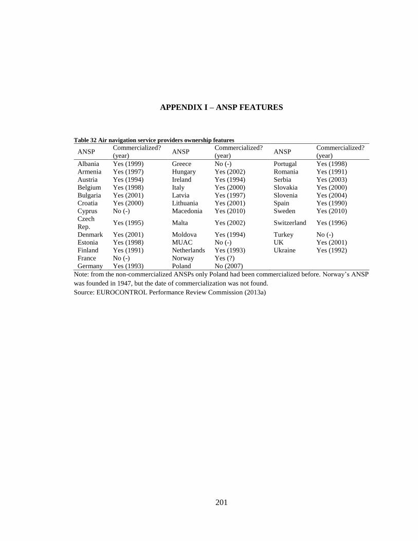
201

APPENDIX I – ANSP FEATURES

Table 32 Air navigation service providers ownership features

ANSP Commercialized?

(year) ANSP

Commercialized?

(year) ANSP

Commercialized?

(year)

Albania Yes (1999) Greece No (-) Portugal Yes (1998)

Armenia Yes (1997) Hungary Yes (2002) Romania Yes (1991)

Austria Yes (1994) Ireland Yes (1994) Serbia Yes (2003)

Belgium Yes (1998) Italy Yes (2000) Slovakia Yes (2000)

Bulgaria Yes (2001) Latvia Yes (1997) Slovenia Yes (2004)

Croatia Yes (2000) Lithuania Yes (2001) Spain Yes (1990)

Cyprus No (-) Macedonia Yes (2010) Sweden Yes (2010)

Czech

Rep. Yes (1995) Malta Yes (2002) Switzerland Yes (1996)

Denmark Yes (2001) Moldova Yes (1994) Turkey No (-)

Estonia Yes (1998) MUAC No (-) UK Yes (2001)

Finland Yes (1991) Netherlands Yes (1993) Ukraine Yes (1992)

France No (-) Norway Yes (?)

Germany Yes (1993) Poland No (2007)

Note: from the non-commercialized ANSPs only Poland had been commercialized before. Norway’s ANSP

was founded in 1947, but the date of commercialization was not found.

Source: EUROCONTROL Performance Review Commission (2013a)

202

APPENDIX II – ANSP DEA ANALYSIS: TABLES

Table 33 DEA efficiency results

Year Country Efficiency Year Country Efficiency Year Country Efficiency

2002 ALB 0.5714 2002 FYROM 0.3095 2005 POL 0.8585

2003 ALB 0.6122 2003 FYROM 0.3214 2006 POL 0.9082

2004 ALB 0.5625 2004 FYROM 0.3766 2007 POL 0.8760

2005 ALB 0.4097 2005 FYROM 0.4026 2008 POL 0.6350

2006 ALB 0.4167 2006 FYROM 0.4286 2009 POL 0.7427

2007 ALB 0.4396 2007 FYROM 0.4286 2010 POL 0.7238

2008 ALB 0.4107 2008 FYROM 0.3571 2011 POL 0.7086

2009 ALB 0.3854 2009 FYROM 0.3896 2002 PT 0.5220

2010 ALB 0.3538 2010 FYROM 0.4286 2003 PT 0.8097

2011 ALB 0.3571 2011 FYROM 0.4143 2004 PT 0.4912

2009 ARM 0.7222 2002 GER 0.9237 2005 PT 0.4980

2010 ARM 0.8194 2003 GER 0.8872 2006 PT 0.5423

2011 ARM 0.7024 2004 GER 0.9118 2007 PT 0.5510

2002 AUS 0.5236 2005 GER 0.9389 2008 PT 0.5154

2003 AUS 0.5209 2006 GER 0.9798 2009 PT 0.5349

2004 AUS 0.5700 2007 GER 1.0000 2010 PT 0.6359

2005 AUS 0.6094 2008 GER 1.0000 2011 PT 0.5876

2006 AUS 0.5723 2009 GER 0.8308 2002 ROM 0.7250

2007 AUS 0.6020 2010 GER 0.8483 2003 ROM 0.6692

2008 AUS 0.5736 2011 GER 0.7863 2004 ROM 0.7282

2009 AUS 0.5272 2003 GRE 0.9823 2005 ROM 0.7202

2010 AUS 0.5101 2004 GRE 1.0000 2006 ROM 0.6569

2011 AUS 0.4831 2005 GRE 0.8208 2007 ROM 0.7279

2002 BEL 0.5673 2006 GRE 0.6100 2008 ROM 0.6465

2003 BEL 0.5439 2007 GRE 0.6884 2009 ROM 0.6779

2004 BEL 0.4852 2008 GRE 0.6257 2010 ROM 0.7638

2005 BEL 0.4626 2009 GRE 0.6410 2011 ROM 0.8050

2006 BEL 0.4583 2010 GRE 0.7088 2006 SER 0.6298

2007 BEL 0.4813 2011 GRE 0.7109 2007 SER 0.9873

2008 BEL 0.4502 2002 HUN 0.6170 2008 SER 0.6395

2009 BEL 0.4254 2003 HUN 0.6748 2009 SER 0.6435

2010 BEL 0.4348 2004 HUN 0.7985 2010 SER 0.6341

2011 BEL 0.4630 2005 HUN 0.8662 2011 SER 0.5673

2002 BUL 0.4895 2006 HUN 0.7688 2002 SK 0.3143

2003 BUL 0.5561 2007 HUN 0.7157 2003 SK 0.3214

2004 BUL 0.5768 2008 HUN 0.6477 2004 SK 0.3542

2005 BUL 0.5750 2009 HUN 0.6176 2005 SK 0.4078

2006 BUL 0.6340 2010 HUN 0.4861 2006 SK 0.4012

2007 BUL 0.7360 2011 HUN 0.7265 2007 SK 0.3900

2008 BUL 0.4928 2002 IRE 0.8734 2008 SK 0.3604

2009 BUL 0.7198 2003 IRE 0.7549 2009 SK 0.3092

203

2010 BUL 0.8068 2004 IRE 0.6653 2010 SK 0.3110

2011 BUL 0.5447 2005 IRE 0.7851 2011 SK 0.4317

2002 CRO 0.5267 2006 IRE 0.7200 2002 SLO 0.3913

2003 CRO 0.7314 2007 IRE 0.7466 2003 SLO 0.4195

2004 CRO 0.5737 2008 IRE 0.6970 2004 SLO 0.5577

2005 CRO 0.6082 2009 IRE 0.6426 2005 SLO 0.4712

2006 CRO 0.5698 2010 IRE 0.5845 2006 SLO 0.4658

2007 CRO 0.6083 2011 IRE 0.5576 2007 SLO 0.4267

2008 CRO 0.6013 2002 ITA 0.8758 2008 SLO 0.3780

2009 CRO 0.5972 2003 ITA 0.7308 2009 SLO 0.3269

2010 CRO 0.5900 2004 ITA 0.6699 2010 SLO 0.3753

2011 CRO 0.5658 2005 ITA 0.6689 2011 SLO 0.3103

2002 CYP 0.8729 2006 ITA 0.7112 2002 SP 0.9512

2003 CYP 0.8220 2007 ITA 0.7492 2003 SP 0.8041

2004 CYP 0.6361 2008 ITA 0.7041 2004 SP 0.7465

2005 CYP 0.6132 2009 ITA 0.6363 2005 SP 0.7552

2006 CYP 0.6033 2010 ITA 0.6642 2006 SP 0.7259

2007 CYP 0.6382 2011 ITA 0.6340 2007 SP 0.7025

2008 CYP 0.6828 2002 LAT 0.4396 2008 SP 0.6226

2009 CYP 0.6350 2003 LAT 0.4490 2009 SP 0.5554

2010 CYP 0.6871 2004 LAT 0.6883 2010 SP 0.7089

2011 CYP 0.7554 2005 LAT 0.6923 2011 SP 0.7512

2002 CZ 0.5771 2006 LAT 0.7157 2002 SWE 0.9561

2003 CZ 0.6337 2007 LAT 0.7410 2003 SWE 0.9848

2004 CZ 0.6915 2008 LAT 0.9105 2004 SWE 1.0000

2005 CZ 0.6578 2009 LAT 0.9495 2005 SWE 1.0000

2006 CZ 0.5746 2010 LAT 0.9741 2006 SWE 0.9748

2007 CZ 0.5175 2011 LAT 1.0000 2007 SWE 0.9052

2008 CZ 0.5023 2002 LIT 0.4470 2008 SWE 0.9079

2009 CZ 0.5261 2003 LIT 0.5069 2009 SWE 0.7806

2010 CZ 0.5032 2004 LIT 0.6026 2010 SWE 0.6246

2011 CZ 0.4812 2005 LIT 0.7239 2011 SWE 0.6841

2002 DEN 0.8827 2006 LIT 0.5962 2002 SWI 0.6102

2003 DEN 0.8326 2007 LIT 0.6852 2003 SWI 0.5509

2004 DEN 0.8105 2008 LIT 0.6976 2004 SWI 0.4859

2005 DEN 0.7919 2009 LIT 0.4276 2005 SWI 0.5619

2006 DEN 0.8857 2010 LIT 0.4826 2006 SWI 0.5322

2007 DEN 0.7342 2011 LIT 0.4951 2007 SWI 0.5423

2008 DEN 0.6751 2002 MAL 0.6375 2008 SWI 0.5372

2009 DEN 0.5769 2003 MAL 0.4762 2009 SWI 0.4822

2010 DEN 0.6121 2004 MAL 0.6326 2010 SWI 0.4357

2011 DEN 0.6619 2005 MAL 0.6042 2011 SWI 0.3901

2002 EC 0.8680 2006 MAL 0.5799 2002 TUR 1.0000

2003 EC 0.8362 2007 MAL 0.5801 2003 TUR 0.6922

2004 EC 0.8846 2008 MAL 0.5801 2004 TUR 0.7072

2005 EC 0.9556 2009 MAL 0.5577 2005 TUR 0.8231

2006 EC 0.9809 2010 MAL 0.6012 2006 TUR 0.8403

2007 EC 1.0000 2011 MAL 0.5810 2007 TUR 0.8921

2008 EC 0.9772 2002 MOL 1.0000 2008 TUR 0.9319

2009 EC 0.8278 2003 MOL 1.0000 2009 TUR 0.9786

2010 EC 0.8210 2004 MOL 0.7143 2010 TUR 1.0000

2011 EC 0.9197 2005 MOL 0.7619 2011 TUR 1.0000

2002 EST 0.9524 2006 MOL 0.7619 2002 UK 1.0000

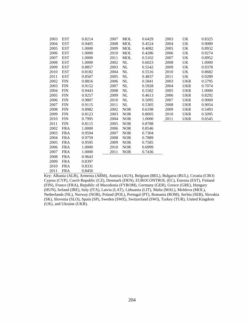
204

2003 EST 0.8214 2007 MOL 0.6429 2003 UK 0.8325

2004 EST 0.9405 2008 MOL 0.4524 2004 UK 0.9089

2005 EST 1.0000 2009 MOL 0.4082 2005 UK 0.8932

2006 EST 1.0000 2010 MOL 0.4286 2006 UK 0.9274

2007 EST 1.0000 2011 MOL 0.5102 2007 UK 0.8952

2008 EST 1.0000 2002 NL 0.6023 2008 UK 1.0000

2009 EST 0.8857 2003 NL 0.5542 2009 UK 0.9378

2010 EST 0.8182 2004 NL 0.5516 2010 UK 0.8682

2011 EST 0.8507 2005 NL 0.4837 2011 UK 0.9289

2002 FIN 0.8816 2006 NL 0.5841 2003 UKR 0.5795

2003 FIN 0.9152 2007 NL 0.5928 2004 UKR 0.7074

2004 FIN 0.9443 2008 NL 0.5582 2005 UKR 1.0000

2005 FIN 0.9257 2009 NL 0.4613 2006 UKR 0.8292

2006 FIN 0.9807 2010 NL 0.5095 2007 UKR 0.9069

2007 FIN 0.9115 2011 NL 0.5305 2008 UKR 0.9054

2008 FIN 0.8982 2002 NOR 0.6198 2009 UKR 0.5493

2009 FIN 0.8123 2003 NOR 0.8005 2010 UKR 0.5095

2010 FIN 0.7995 2004 NOR 1.0000 2011 UKR 0.6545

2011 FIN 0.8115 2005 NOR 0.8788

2002 FRA 1.0000 2006 NOR 0.8546

2003 FRA 0.9594 2007 NOR 0.7304

2004 FRA 0.9759 2008 NOR 0.7889

2005 FRA 0.9595 2009 NOR 0.7585

2006 FRA 1.0000 2010 NOR 0.6999

2007 FRA 1.0000 2011 NOR 0.7436

2008 FRA 0.9643

2009 FRA 0.8397

2010 FRA 0.8331

2011 FRA 0.8450

Key: Albania (ALB), Armenia (ARM), Austria (AUS), Belgium (BEL), Bulgaria (BUL), Croatia (CRO)

Cyprus (CYP), Czech Republic (CZ), Denmark (DEN), EUROCONTROL (EC), Estonia (EST), Finland

(FIN), France (FRA), Republic of Macedonia (FYROM), Germany (GER), Greece (GRE), Hungary

(HUN), Ireland (IRE), Italy (ITA), Latvia (LAT), Lithuania (LIT), Malta (MAL), Moldova (MOL),

Netherlands (NL), Norway (NOR), Poland (POL), Portugal (PT), Romania (ROM), Serbia (SEB), Slovakia

(SK), Slovenia (SLO), Spain (SP), Sweden (SWE), Switzerland (SWI), Turkey (TUR), United Kingdom

(UK), and Ukraine (UKR).

205

Table 34 DEA allocative efficiency results

Year Country Efficiency Year Country Efficiency Year Country Efficiency

2002 ALB 0.9412 2002 FYROM 1.0000 2005 POL 0.9390

2003 ALB 0.7778 2003 FYROM 0.9600 2006 POL 0.9254

2004 ALB 0.7619 2004 FYROM 0.9565 2007 POL 0.9121

2005 ALB 0.9231 2005 FYROM 0.9565 2008 POL 0.9751

2006 ALB 0.9231 2006 FYROM 0.9524 2009 POL 0.9691

2007 ALB 0.8966 2007 FYROM 0.9524 2010 POL 0.9662

2008 ALB 0.9333 2008 FYROM 0.9600 2011 POL 0.9815

2009 ALB 0.9412 2009 FYROM 0.9167 2002 PT 0.9916

2010 ALB 0.9744 2010 FYROM 0.9091 2003 PT 0.9727

2011 ALB 0.9524 2011 FYROM 0.9091 2004 PT 0.9867

2009 ARM 0.9231 2002 GER 0.9070 2005 PT 0.9854

2010 ARM 0.9231 2003 GER 0.8953 2006 PT 0.9850

2011 ARM 1.0000 2004 GER 0.8934 2007 PT 0.9865

2002 AUS 0.9245 2005 GER 0.8994 2008 PT 0.9889

2003 AUS 0.9295 2006 GER 0.9157 2009 PT 0.9863

2004 AUS 0.9268 2007 GER 1.0000 2010 PT 0.9778

2005 AUS 0.9266 2008 GER 1.0000 2011 PT 0.9878

2006 AUS 0.9487 2009 GER 0.9980 2002 ROM 0.9039

2007 AUS 0.9464 2010 GER 0.9941 2003 ROM 0.9361

2008 AUS 0.9540 2011 GER 0.9957 2004 ROM 0.9490

2009 AUS 0.9600 2003 GRE 0.9850 2005 ROM 0.9643

2010 AUS 0.9596 2004 GRE 1.0000 2006 ROM 0.9644

2011 AUS 0.9635 2005 GRE 0.9944 2007 ROM 0.9764

2002 BEL 0.8492 2006 GRE 0.9989 2008 ROM 0.9749

2003 BEL 0.8387 2007 GRE 0.9977 2009 ROM 0.9762

2004 BEL 0.8449 2008 GRE 0.9509 2010 ROM 0.9778

2005 BEL 0.8370 2009 GRE 0.9510 2011 ROM 0.9843

2006 BEL 0.8538 2010 GRE 0.9472 2006 SER 0.9001

2007 BEL 0.8431 2011 GRE 0.9516 2007 SER 0.9417

2008 BEL 0.8564 2002 HUN 0.9636 2008 SER 0.9787

2009 BEL 0.8550 2003 HUN 0.9392 2009 SER 0.9840

2010 BEL 0.8483 2004 HUN 0.9379 2010 SER 0.9685

2011 BEL 0.8646 2005 HUN 0.9423 2011 SER 0.9680

2002 BUL 0.9584 2006 HUN 0.9460 2002 SK 0.9615

2003 BUL 0.9447 2007 HUN 0.9577 2003 SK 0.9492

2004 BUL 0.9423 2008 HUN 0.9686 2004 SK 0.9546

2005 BUL 0.9506 2009 HUN 0.9610 2005 SK 0.9606

2006 BUL 0.9491 2010 HUN 0.9782 2006 SK 0.9516

2007 BUL 0.9492 2011 HUN 0.9857 2007 SK 0.9691

2008 BUL 0.9460 2002 IRE 0.9351 2008 SK 0.9684

2009 BUL 0.9504 2003 IRE 0.9581 2009 SK 0.9546

2010 BUL 0.9467 2004 IRE 0.9638 2010 SK 0.9540

2011 BUL 0.9441 2005 IRE 0.9600 2011 SK 0.9649

2002 CRO 0.9620 2006 IRE 0.9614 2002 SLO 0.9608

2003 CRO 0.9518 2007 IRE 0.9613 2003 SLO 0.9283

2004 CRO 0.9650 2008 IRE 0.9628 2004 SLO 0.9286

2005 CRO 0.9639 2009 IRE 0.9539 2005 SLO 0.9116

2006 CRO 0.9598 2010 IRE 0.9554 2006 SLO 0.9181

2007 CRO 0.9806 2011 IRE 0.9639 2007 SLO 0.9394

2008 CRO 0.9596 2002 ITA 0.9347 2008 SLO 0.9329

2009 CRO 0.9834 2003 ITA 0.9510 2009 SLO 0.9485

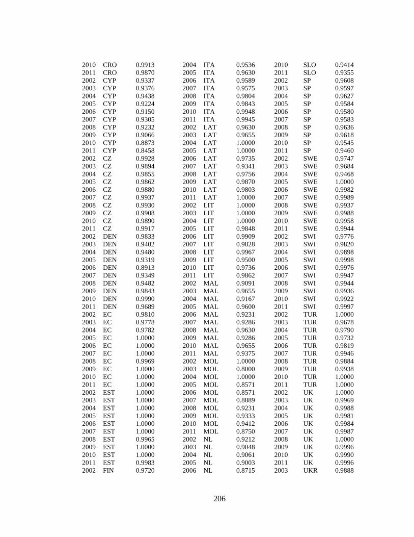
206

2010 CRO 0.9913 2004 ITA 0.9536 2010 SLO 0.9414

2011 CRO 0.9870 2005 ITA 0.9630 2011 SLO 0.9355

2002 CYP 0.9337 2006 ITA 0.9589 2002 SP 0.9608

2003 CYP 0.9376 2007 ITA 0.9575 2003 SP 0.9597

2004 CYP 0.9438 2008 ITA 0.9804 2004 SP 0.9627

2005 CYP 0.9224 2009 ITA 0.9843 2005 SP 0.9584

2006 CYP 0.9150 2010 ITA 0.9948 2006 SP 0.9580

2007 CYP 0.9305 2011 ITA 0.9945 2007 SP 0.9583

2008 CYP 0.9232 2002 LAT 0.9630 2008 SP 0.9636

2009 CYP 0.9066 2003 LAT 0.9655 2009 SP 0.9618

2010 CYP 0.8873 2004 LAT 1.0000 2010 SP 0.9545

2011 CYP 0.8458 2005 LAT 1.0000 2011 SP 0.9460

2002 CZ 0.9928 2006 LAT 0.9735 2002 SWE 0.9747

2003 CZ 0.9894 2007 LAT 0.9341 2003 SWE 0.9684

2004 CZ 0.9855 2008 LAT 0.9756 2004 SWE 0.9468

2005 CZ 0.9862 2009 LAT 0.9870 2005 SWE 1.0000

2006 CZ 0.9880 2010 LAT 0.9803 2006 SWE 0.9982

2007 CZ 0.9937 2011 LAT 1.0000 2007 SWE 0.9989

2008 CZ 0.9930 2002 LIT 1.0000 2008 SWE 0.9937

2009 CZ 0.9908 2003 LIT 1.0000 2009 SWE 0.9988

2010 CZ 0.9890 2004 LIT 1.0000 2010 SWE 0.9958

2011 CZ 0.9917 2005 LIT 0.9848 2011 SWE 0.9944

2002 DEN 0.9833 2006 LIT 0.9909 2002 SWI 0.9776

2003 DEN 0.9402 2007 LIT 0.9828 2003 SWI 0.9820

2004 DEN 0.9480 2008 LIT 0.9967 2004 SWI 0.9898

2005 DEN 0.9319 2009 LIT 0.9500 2005 SWI 0.9998

2006 DEN 0.8913 2010 LIT 0.9736 2006 SWI 0.9976

2007 DEN 0.9349 2011 LIT 0.9862 2007 SWI 0.9947

2008 DEN 0.9482 2002 MAL 0.9091 2008 SWI 0.9944

2009 DEN 0.9843 2003 MAL 0.9655 2009 SWI 0.9936

2010 DEN 0.9990 2004 MAL 0.9167 2010 SWI 0.9922

2011 DEN 0.9689 2005 MAL 0.9600 2011 SWI 0.9997

2002 EC 0.9810 2006 MAL 0.9231 2002 TUR 1.0000

2003 EC 0.9778 2007 MAL 0.9286 2003 TUR 0.9678

2004 EC 0.9782 2008 MAL 0.9630 2004 TUR 0.9790

2005 EC 1.0000 2009 MAL 0.9286 2005 TUR 0.9732

2006 EC 1.0000 2010 MAL 0.9655 2006 TUR 0.9819

2007 EC 1.0000 2011 MAL 0.9375 2007 TUR 0.9946

2008 EC 0.9969 2002 MOL 1.0000 2008 TUR 0.9884

2009 EC 1.0000 2003 MOL 0.8000 2009 TUR 0.9938

2010 EC 1.0000 2004 MOL 1.0000 2010 TUR 1.0000

2011 EC 1.0000 2005 MOL 0.8571 2011 TUR 1.0000

2002 EST 1.0000 2006 MOL 0.8571 2002 UK 1.0000

2003 EST 1.0000 2007 MOL 0.8889 2003 UK 0.9969

2004 EST 1.0000 2008 MOL 0.9231 2004 UK 0.9988

2005 EST 1.0000 2009 MOL 0.9333 2005 UK 0.9981

2006 EST 1.0000 2010 MOL 0.9412 2006 UK 0.9984

2007 EST 1.0000 2011 MOL 0.8750 2007 UK 0.9987

2008 EST 0.9965 2002 NL 0.9212 2008 UK 1.0000

2009 EST 1.0000 2003 NL 0.9048 2009 UK 0.9996

2010 EST 1.0000 2004 NL 0.9061 2010 UK 0.9990

2011 EST 0.9983 2005 NL 0.9003 2011 UK 0.9996

2002 FIN 0.9720 2006 NL 0.8715 2003 UKR 0.9888

207

2003 FIN 0.9549 2007 NL 0.8697 2004 UKR 0.9994

2004 FIN 0.9566 2008 NL 0.8670 2005 UKR 1.0000

2005 FIN 0.9496 2009 NL 0.8831 2006 UKR 0.9828

2006 FIN 0.9479 2010 NL 0.8796 2007 UKR 0.9795

2007 FIN 0.9528 2011 NL 0.9245 2008 UKR 0.9830

2008 FIN 0.9559 2002 NOR 0.9899 2009 UKR 0.9936

2009 FIN 0.9585 2003 NOR 0.9954 2010 UKR 0.9920

2010 FIN 0.9585 2004 NOR 1.0000 2011 UKR 0.9560

2011 FIN 0.9650 2005 NOR 0.9990

2002 FRA 1.0000 2006 NOR 0.9983

2003 FRA 0.9980 2007 NOR 0.9965

2004 FRA 0.9970 2008 NOR 0.9991

2005 FRA 0.9993 2009 NOR 0.9976

2006 FRA 1.0000 2010 NOR 0.9979

2007 FRA 1.0000 2011 NOR 0.9948

2008 FRA 0.9973

2009 FRA 0.9963

2010 FRA 0.9853

2011 FRA 0.9873

Key: Albania (ALB), Armenia (ARM), Austria (AUS), Belgium (BEL), Bulgaria (BUL), Croatia (CRO)

Cyprus (CYP), Czech Republic (CZ), Denmark (DEN), EUROCONTROL (EC), Estonia (EST), Finland

(FIN), France (FRA), Republic of Macedonia (FYROM), Germany (GER), Greece (GRE), Hungary

(HUN), Ireland (IRE), Italy (ITA), Latvia (LAT), Lithuania (LIT), Malta (MAL), Moldova (MOL),

Netherlands (NL), Norway (NOR), Poland (POL), Portugal (PT), Romania (ROM), Serbia (SEB), Slovakia

(SK), Slovenia (SLO), Spain (SP), Sweden (SWE), Switzerland (SWI), Turkey (TUR), United Kingdom

(UK), and Ukraine (UKR).

208

Table 35 DEA inputs and outputs slacks

Year Country

Slacks

Provision

costs

Other

costs

IFR flight

hours

Airport

movements 1/delays

2002 ALB 0.5714 0.0000 0.0000 7.8163 0.0000

2003 ALB 2.4490 0.0000 0.0000 6.8367 0.0000

2004 ALB 2.8125 0.0000 0.0000 9.0000 0.5833

2005 ALB 0.8194 0.0000 0.0000 8.0000 0.5083

2006 ALB 0.8333 0.0000 0.0000 4.2857 0.0000

2007 ALB 1.3187 0.0000 0.0000 4.7347 0.0000

2008 ALB 0.8214 0.0000 0.0000 9.0000 0.5250

2009 ALB 0.7708 0.0000 0.0000 10.0000 0.5119

2010 ALB 0.3538 0.0000 0.0000 12.6667 0.4861

2011 ALB 0.7143 0.0000 0.0000 11.5714 0.4896

2009 ARM 0.7222 0.0000 10.3333 0.0000 0.0000

2010 ARM 0.8194 0.0000 12.4167 0.0000 0.0000

2011 ARM 0.0000 0.0000 10.4167 0.0000 0.0000

2002 AUS 10.3299 0.0000 0.0000 0.0000 0.4135

2003 AUS 9.9628 0.0000 0.0000 0.0000 0.3963

2004 AUS 11.3762 0.0000 0.0000 0.0000 0.3404

2005 AUS 12.1949 0.0000 0.0000 0.0000 0.2818

2006 AUS 8.0092 0.0000 0.0000 0.0000 0.2552

2007 AUS 9.0206 0.0000 0.0000 0.0000 0.1908

2008 AUS 7.6591 0.0000 0.0000 0.0000 0.1570

2009 AUS 5.6905 0.0000 0.0000 0.0000 0.2486

2010 AUS 5.8408 0.0000 0.0000 0.0000 0.2480

2011 AUS 4.9314 0.0000 0.0000 0.0000 0.2538

2002 BEL 24.3818 0.0000 72.0000 0.0000 0.3488

2003 BEL 26.8520 0.0000 75.0000 0.0000 0.3452

2004 BEL 24.1540 0.0000 62.5000 0.0000 0.3918

2005 BEL 24.8081 0.0000 65.0000 0.0000 0.4111

2006 BEL 23.2523 0.0000 71.0000 0.0000 0.3747

2007 BEL 25.9833 0.0000 69.0000 0.0000 0.3561

2008 BEL 23.4656 0.0000 63.5000 0.0000 0.3571

2009 BEL 22.5662 0.0000 63.5000 0.0000 0.3888

2010 BEL 24.0103 0.0000 66.0000 0.0000 0.3843

2011 BEL 22.6972 0.0000 76.0000 0.0000 0.3295

2002 BUL 3.3209 0.0000 0.0000 22.5503 0.0000

2003 BUL 4.2119 0.0000 0.0000 12.5079 0.0000

2004 BUL 4.7946 0.0000 0.0000 13.7672 0.0000

2005 BUL 4.4871 0.0000 0.0000 12.2434 0.0000

2006 BUL 4.9725 0.0000 0.0000 3.5026 0.0000

2007 BUL 5.6825 0.0000 0.0000 0.0000 0.0000

2008 BUL 3.5219 0.0000 0.0000 0.0000 0.2482

2009 BUL 5.9604 0.0000 0.0000 6.1058 0.0000

2010 BUL 6.8372 0.0000 0.0000 22.9735 0.0000

2011 BUL 4.2426 0.0000 0.0000 0.0000 0.6863

2002 CRO 1.2715 0.0000 0.0000 0.0000 0.5784

2003 CRO 2.9597 0.0000 0.0000 3.3810 0.0000

2004 CRO 1.4407 0.0000 0.0000 0.0000 0.7311

2005 CRO 1.7618 0.0000 0.0000 0.0000 0.8085

2006 CRO 1.9851 0.0000 0.0000 0.0000 0.8094

209

2007 CRO 0.7377 0.0000 0.0000 0.0000 0.7624

2008 CRO 2.4497 0.0000 0.0000 0.0000 0.7532

2009 CRO 0.6062 0.0000 0.0000 0.0000 0.7363

2010 CRO 0.0286 0.0000 0.0000 0.0000 0.7167

2011 CRO 0.4625 0.0000 0.0000 0.0000 0.6895

2002 CYP 2.3078 0.0000 0.0000 0.0000 0.9084

2003 CYP 2.2552 0.0000 0.0000 0.0000 0.8707

2004 CYP 2.0586 0.0000 0.0000 0.0000 0.8938

2005 CYP 3.1246 0.0000 0.0000 0.0000 0.8941

2006 CYP 3.6478 0.0000 0.0000 0.0000 0.8855

2007 CYP 3.2183 0.0000 0.0000 0.0000 0.8675

2008 CYP 4.0967 0.0000 0.0000 0.0000 0.8422

2009 CYP 5.0709 0.0000 0.0000 0.0000 0.8471

2010 CYP 6.8600 0.0000 0.0000 0.0000 0.8290

2011 CYP 9.9489 0.0000 0.0000 0.0000 0.8298

2002 CZ 0.0000 0.0000 0.0000 0.0000 0.7676

2003 CZ 0.0000 0.0000 0.0000 0.0000 0.7335

2004 CZ 0.0000 0.0000 0.0000 0.0000 0.6653

2005 CZ 0.0000 0.0000 0.0000 0.0000 0.6232

2006 CZ 0.0000 0.0000 0.0000 0.0000 0.5969

2007 CZ 0.0000 0.0000 0.0000 0.0000 0.5517

2008 CZ 0.0000 0.0000 0.0000 0.0000 0.5211

2009 CZ 0.0000 0.0000 0.0000 0.0000 0.5509

2010 CZ 0.0000 0.0000 0.0000 0.0000 0.5492

2011 CZ 0.0000 0.0000 0.0000 0.0000 0.4968

2002 DEN 2.2378 0.0000 0.0000 0.0000 0.3816

2003 DEN 8.6580 0.0000 0.0000 0.0000 0.3887

2004 DEN 7.8842 0.0000 0.0000 0.0000 0.3499

2005 DEN 10.1820 0.0000 0.0000 0.0000 0.3724

2006 DEN 16.9197 0.0000 0.0000 0.0000 0.3871

2007 DEN 9.7120 0.0000 0.0000 0.0000 0.3640

2008 DEN 7.7093 0.0000 0.0000 0.0000 0.3567

2009 DEN 1.7968 0.0000 0.0000 0.0000 0.4016

2010 DEN 0.0000 0.0000 0.0000 0.0000 0.3772

2011 DEN 0.0000 4.6006 0.0000 0.0000 0.1605

2002 EC 3.4718 0.0000 0.0000 9.8752 0.2814

2003 EC 4.1809 0.0000 0.0000 9.0691 0.2581

2004 EC 4.4229 0.0000 0.0000 6.8522 0.1948

2005 EC 0.0000 0.0000 0.0000 4.3666 0.1166

2006 EC 0.0000 0.0000 0.0000 1.9482 0.0536

2007 EC 0.0000 0.0000 0.0000 0.0000 0.0000

2008 EC 0.0000 0.7775 0.0000 7.3431 0.0000

2009 EC 0.0000 0.0000 0.0000 2.8887 0.0654

2010 EC 0.0000 0.0000 0.0000 2.1497 0.0491

2011 EC 0.0000 0.0000 0.0000 0.7390 0.0067

2002 EST 0.0000 0.0000 8.6667 0.0000 0.0000

2003 EST 0.0000 0.0000 0.0000 1.0000 0.1250

2004 EST 0.0000 0.0000 0.0000 4.0000 0.0417

2005 EST 0.0000 0.0000 0.0000 0.0000 0.0000

2006 EST 0.0000 0.0000 0.0000 0.0000 0.0000

2007 EST 0.0000 0.0000 0.0000 0.0000 0.0000

2008 EST 0.0000 0.0000 0.0000 0.0000 0.0000

2009 EST 0.0000 0.0000 0.0000 5.5102 0.0000

210

2010 EST 0.0000 0.0000 0.0000 4.0000 0.8000

2011 EST 0.0000 0.0000 0.0000 0.0000 0.5012

2002 FIN 2.9104 0.0000 23.5000 0.0000 0.3767

2003 FIN 4.4188 0.0000 13.5000 0.0000 0.4363

2004 FIN 4.4695 0.0000 17.0000 0.0000 0.5374

2005 FIN 5.2286 0.0000 15.0000 0.0000 0.5256

2006 FIN 5.6159 0.0000 22.0000 0.0000 0.4610

2007 FIN 4.9881 0.0000 20.0000 0.0000 0.4826

2008 FIN 4.7581 0.0000 19.0000 0.0000 0.4788

2009 FIN 4.1754 0.0000 18.5000 0.0000 0.4739

2010 FIN 4.1125 0.0000 14.5000 0.0000 0.5335

2011 FIN 3.8098 0.0000 13.5000 0.0000 0.5197

2002 FRA 0.0000 0.0000 0.0000 0.0000 0.0000

2003 FRA 0.0000 0.0000 0.0000 0.0000 0.0001

2004 FRA 0.0000 3.6537 0.0000 0.0000 0.0000

2005 FRA 0.0000 0.0000 0.0000 0.0000 0.0000

2006 FRA 0.0000 0.0000 0.0000 0.0000 0.0000

2007 FRA 0.0000 0.0000 0.0000 0.0000 0.0000

2008 FRA 0.0000 6.4100 0.0000 5.1544 0.0000

2009 FRA 0.0000 7.8888 0.0000 19.1537 0.0000

2010 FRA 31.1216 0.0000 0.0000 0.2152 0.0004

2011 FRA 26.4506 0.0000 0.0000 0.0000 0.0000

2002 FYROM 0.0000 0.0000 0.0000 1.8776 0.0000

2003 FYROM 0.3214 0.0000 0.0000 3.3673 0.0000

2004 FYROM 0.3766 0.0000 0.0000 6.3469 0.0000

2005 FYROM 0.4026 0.0000 0.0000 6.3265 0.0000

2006 FYROM 0.4286 0.0000 0.0000 5.8367 0.0000

2007 FYROM 0.4286 0.0000 0.0000 5.8367 0.0000

2008 FYROM 0.3571 0.0000 0.0000 4.8367 0.0000

2009 FYROM 0.7792 0.0000 0.0000 6.8367 0.0000

2010 FYROM 0.8571 0.0000 0.0000 5.8367 0.0000

2011 FYROM 0.8286 0.0000 0.0000 6.3469 0.0000

2002 GER 141.9356 0.0000 0.0000 0.0000 0.0006

2003 GER 163.5118 0.0000 0.0000 0.0000 0.0008

2004 GER 173.7552 0.0000 0.0000 0.0000 0.0002

2005 GER 168.8701 0.0000 0.0000 0.0000 0.0000

2006 GER 143.2576 0.0000 0.0000 0.0000 0.0000

2007 GER 0.0000 0.0000 0.0000 0.0000 0.0000

2008 GER 0.0000 0.0000 0.0000 0.0000 0.0000

2009 GER 0.0000 2.9142 0.0000 0.0000 0.0003

2010 GER 0.0000 8.7779 0.0000 0.0000 0.0004

2011 GER 0.0000 6.6225 0.0000 0.0000 0.0002

2003 GRE 1.0060 0.0000 0.0000 0.0000 0.0796

2004 GRE 0.0000 0.0000 0.0000 0.0000 0.0000

2005 GRE 0.3552 0.0000 0.0000 0.0000 0.0317

2006 GRE 0.0000 0.0000 0.0000 0.0000 0.0011

2007 GRE 0.0000 0.0000 0.0000 0.0000 0.0015

2008 GRE 10.5716 0.0000 0.0000 0.0000 0.0524

2009 GRE 9.8819 0.0000 0.0000 0.0000 0.0673

2010 GRE 11.7570 0.0000 0.0000 0.0000 0.0476

2011 GRE 9.7609 0.0000 0.0000 0.0000 0.0764

2002 HUN 1.8092 0.0000 0.0000 0.0000 0.3064

2003 HUN 3.7885 0.0000 0.0000 0.0000 0.6380

211

2004 HUN 4.6541 0.0000 0.0000 0.0000 0.7045

2005 HUN 4.7124 0.0000 0.0000 0.0000 0.6614

2006 HUN 4.3773 0.0000 0.0000 0.0000 0.6222

2007 HUN 3.1533 0.0000 0.0000 0.0000 0.6027

2008 HUN 2.0636 0.0000 0.0000 0.0000 0.5442

2009 HUN 2.7937 0.0000 0.0000 0.0000 0.6405

2010 HUN 1.1114 0.0000 0.0000 0.0000 0.1750

2011 HUN 2.0938 0.0000 0.0000 10.1852 0.0000

2002 IRE 6.7150 0.0000 0.0000 0.0000 0.5338

2003 IRE 3.9700 0.0000 0.0000 0.0000 0.5251

2004 IRE 3.2120 0.0000 0.0000 0.0000 0.5332

2005 IRE 3.8498 0.0000 0.0000 0.0000 0.4277

2006 IRE 3.7695 0.0000 0.0000 0.0000 0.3901

2007 IRE 4.0073 0.0000 0.0000 0.0000 0.3357

2008 IRE 3.6781 0.0000 0.0000 0.0000 0.3693

2009 IRE 4.4653 0.0000 0.0000 0.0000 0.4199

2010 IRE 4.1386 0.0000 0.0000 0.0000 0.4668

2011 IRE 3.0188 0.0000 0.0000 0.0000 0.2286

2002 ITA 67.6169 0.0000 0.0000 0.0000 0.0021

2003 ITA 46.9752 0.0000 0.0000 0.0000 0.0013

2004 ITA 43.4242 0.0000 0.0000 0.0000 0.0014

2005 ITA 33.1360 0.0000 0.0000 0.0000 0.0011

2006 ITA 38.1894 0.0000 0.0000 0.0000 0.0008

2007 ITA 42.9380 0.0000 0.0000 0.0000 0.0003

2008 ITA 17.9525 0.0000 0.0000 0.0000 0.0000

2009 ITA 13.2319 0.0000 0.0000 0.0000 0.0000

2010 ITA 2.8570 0.0000 0.0000 0.0000 0.0000

2011 ITA 3.7996 0.0000 0.0000 0.0000 0.0000

2002 LAT 0.4396 0.0000 0.0000 6.7347 0.0000

2003 LAT 0.4490 0.0000 0.0000 7.6939 0.0000

2004 LAT 0.0000 0.0000 0.0000 4.1020 0.0000

2005 LAT 0.0000 0.0000 1.0000 0.0000 0.0000

2006 LAT 0.5887 0.0000 0.0000 3.4339 0.0000

2007 LAT 1.9056 0.0000 0.0000 0.0847 0.0000

2008 LAT 0.9786 0.0000 0.0000 0.0000 0.0000

2009 LAT 0.0000 0.5300 5.1622 0.0000 0.0000

2010 LAT 0.0000 0.8615 4.6216 0.0000 0.0000

2011 LAT 0.0000 0.0000 0.0000 0.0000 0.0000

2002 LIT 0.0000 0.0000 2.4167 0.0000 0.0000

2003 LIT 0.0000 0.0000 10.5833 0.0000 0.0000

2004 LIT 0.0000 0.0000 17.8333 0.0000 0.0000

2005 LIT 0.3185 0.0000 23.4595 0.0000 0.0000

2006 LIT 0.1908 0.0000 19.4595 0.0000 0.0000

2007 LIT 0.4245 0.0000 15.4054 0.0000 0.0000

2008 LIT 0.0000 0.0914 9.3514 0.0000 0.0000

2009 LIT 0.8553 0.0000 4.8750 0.0000 0.0000

2010 LIT 0.5598 0.0000 7.4595 0.0000 0.0000

2011 LIT 0.3145 0.0000 4.4324 0.0000 0.0000

2002 MAL 1.2750 0.0000 9.6250 0.0000 0.0000

2003 MAL 0.4762 0.0000 5.6667 0.0000 0.0000

2004 MAL 1.2652 0.0000 8.7083 0.0000 0.0000

2005 MAL 0.6042 0.0000 9.7500 0.0000 0.0000

2006 MAL 1.1597 0.0000 6.7083 0.0000 0.0000

212

2007 MAL 1.1603 0.0000 5.7917 0.0000 0.0000

2008 MAL 0.5801 0.0000 2.7917 0.0000 0.0000

2009 MAL 1.1154 0.0000 0.7500 0.0000 0.0000

2010 MAL 0.6012 0.0000 2.9167 0.0000 0.0000

2011 MAL 1.1619 0.0000 0.0000 1.0204 0.0000

2002 MOL 0.0000 0.0000 0.0000 0.0000 0.0000

2003 MOL 1.0000 0.0000 0.0000 1.0000 0.0000

2004 MOL 0.0000 0.0000 0.0000 0.4898 0.0000

2005 MOL 0.7619 0.0000 0.0000 0.9796 0.0000

2006 MOL 0.7619 0.0000 0.0000 1.9796 0.0000

2007 MOL 0.6429 0.0000 0.0000 0.9592 0.0000

2008 MOL 0.4524 0.0000 0.0000 0.4490 0.0000

2009 MOL 0.4082 0.0000 0.0000 1.9388 0.0000

2010 MOL 0.4286 0.0000 0.0000 1.8980 0.0000

2011 MOL 1.0204 0.0000 0.0000 1.3878 0.0000

2002 NL 16.9944 0.0000 109.5000 0.0000 0.0833

2003 NL 18.2634 0.0000 81.5000 0.0000 0.2000

2004 NL 18.4848 0.0000 89.0000 0.0000 0.1766

2005 NL 19.6800 0.0000 93.0000 0.0000 0.1800

2006 NL 27.3118 0.0000 93.0000 0.0000 0.1411

2007 NL 28.7426 0.0000 99.5000 0.0000 0.1144

2008 NL 28.9590 0.0000 95.5000 0.0000 0.1291

2009 NL 22.8071 0.0000 84.0000 0.0000 0.2000

2010 NL 23.4400 0.0000 80.5000 0.0000 0.2116

2011 NL 15.0959 0.0000 87.5000 0.0000 0.1472

2002 NOR 0.0000 2.0057 15.5000 0.0000 0.0401

2003 NOR 0.9194 0.0000 3.2647 0.0000 0.0000

2004 NOR 0.0000 0.0000 0.0000 0.0000 0.0000

2005 NOR 0.0000 0.2102 0.0000 0.0000 0.0018

2006 NOR 0.0000 0.4169 9.5196 0.0000 0.0000

2007 NOR 0.0000 0.9301 7.9470 0.0000 0.0006

2008 NOR 0.0000 0.2418 2.1003 0.0000 0.0000

2009 NOR 0.0000 0.6002 0.0000 0.0000 0.0000

2010 NOR 0.0000 0.5340 0.0000 0.0000 0.0000

2011 NOR 0.0000 1.5173 0.0000 0.0000 0.0030

2005 POL 6.6746 0.0000 0.0000 0.0000 0.4841

2006 POL 10.3567 0.0000 0.0000 0.0000 0.3822

2007 POL 14.3584 0.0000 0.0000 0.0000 0.3022

2008 POL 1.4731 0.0000 0.0000 0.0000 0.2433

2009 POL 2.5823 0.0000 0.0000 0.0000 0.3044

2010 POL 3.4296 0.0000 0.0000 0.0000 0.2599

2011 POL 0.4973 0.0000 0.0000 0.0000 0.1819

2002 PT 0.0000 0.0000 0.0000 0.0000 0.3795

2003 PT 0.0000 5.4648 9.8108 0.0000 0.0000

2004 PT 0.0000 0.0000 0.0000 0.0000 0.4368

2005 PT 0.0000 0.0000 0.0000 0.0000 0.3269

2006 PT 0.0000 0.0000 0.0000 0.0000 0.3970

2007 PT 0.0000 0.0000 0.0000 0.0000 0.3919

2008 PT 0.0000 0.0000 0.0000 0.0000 0.3623

2009 PT 0.0000 0.0000 0.0000 0.0000 0.4004

2010 PT 1.0682 0.0000 0.0000 0.0000 0.3795

2011 PT 0.0000 0.0000 0.0000 0.0000 0.3452

2002 ROM 14.6288 0.0000 0.0000 47.9259 0.0000

213

2003 ROM 10.5655 0.0000 0.0000 46.4868 0.0000

2004 ROM 9.6106 0.0000 0.0000 41.9153 0.0000

2005 ROM 7.4764 0.0000 0.0000 42.9477 0.0000

2006 ROM 7.4618 0.0000 0.0000 30.9477 0.0000

2007 ROM 4.9853 0.0000 0.0000 11.6471 0.0000

2008 ROM 5.5760 0.0000 0.0000 29.8954 0.0000

2009 ROM 5.0880 0.0000 0.0000 11.9216 0.0000

2010 ROM 5.2161 0.0000 0.0000 35.4183 0.0000

2011 ROM 3.7648 0.0000 0.0000 56.9673 0.0000

2006 SER 7.5430 0.0000 0.0000 0.0000 0.2666

2007 SER 8.5812 0.0000 0.0000 52.5344 0.0000

2008 SER 1.4492 0.0000 0.0000 0.0000 0.3489

2009 SER 1.0200 0.0000 0.0000 0.0000 0.1797

2010 SER 2.5769 0.0000 0.0000 0.0000 0.4574

2011 SER 2.6682 0.0000 0.0000 0.0000 0.6158

2002 SK 0.6286 0.0000 0.0000 7.0816 0.0000

2003 SK 0.9643 0.0000 0.0000 7.0000 0.9804

2004 SK 1.0382 0.0000 0.0000 0.0000 0.9627

2005 SK 1.0149 0.0000 0.0000 0.0000 0.9529

2006 SK 1.3101 0.0000 0.0000 0.0000 0.9203

2007 SK 0.7564 0.0000 0.0000 0.0000 0.9496

2008 SK 0.8469 0.0000 0.0000 0.0000 0.9154

2009 SK 1.2838 0.0000 0.0000 0.0000 0.8767

2010 SK 1.4383 0.0000 0.0000 0.0000 0.9167

2011 SK 1.6377 0.0000 0.0000 19.2540 0.0000

2002 SLO 0.3832 0.0000 0.0000 0.0000 0.7002

2003 SLO 0.7821 0.0000 0.0000 0.0000 0.5875

2004 SLO 1.1154 0.0000 13.7500 0.0000 0.0000

2005 SLO 1.2917 0.0000 0.0000 0.0000 0.6398

2006 SLO 1.2593 0.0000 0.0000 0.0000 0.4744

2007 SLO 1.0607 0.0000 0.0000 0.0000 0.5916

2008 SLO 1.2681 0.0000 0.0000 0.0000 0.4344

2009 SLO 0.8590 0.0000 0.0000 0.0000 0.2887

2010 SLO 1.2308 0.0000 11.9730 0.0000 0.0000

2011 SLO 1.2414 0.0000 7.0000 0.0000 0.0000

2002 SP 47.2991 0.0000 0.0000 0.0000 0.0014

2003 SP 49.8314 0.0000 0.0000 0.0000 0.0002

2004 SP 49.3899 0.0000 0.0000 0.0000 0.0008

2005 SP 59.9431 0.0000 0.0000 0.0000 0.0006

2006 SP 63.8353 0.0000 0.0000 0.0000 0.0003

2007 SP 65.5814 0.0000 0.0000 0.0000 0.0000

2008 SP 57.1774 0.0000 0.0000 0.0000 0.0000

2009 SP 52.7774 0.0000 0.0000 0.0000 0.0007

2010 SP 63.3464 0.0000 0.0000 0.0000 0.0011

2011 SP 77.9457 0.0000 0.0000 0.0000 0.0005

2002 SWE 0.0000 0.0000 0.0000 0.0000 0.0000

2003 SWE 0.0000 0.0000 0.0000 0.0000 0.0000

2004 SWE 0.0000 0.0000 0.0000 0.0000 0.0000

2005 SWE 0.0000 0.0000 0.0000 0.0000 0.0000

2006 SWE 0.0000 0.3535 0.0000 0.0000 0.0000

2007 SWE 0.0000 0.2014 0.0000 0.0000 0.0002

2008 SWE 0.0000 1.6386 0.0000 0.0000 0.0000

2009 SWE 0.0000 0.1853 0.0000 0.0000 0.0000

214

2010 SWE 0.0000 0.8654 0.0000 0.0000 0.0000

2011 SWE 0.0000 1.4734 0.0000 0.0000 0.0000

2002 SWI 3.4181 0.0000 0.0000 0.0000 0.1036

2003 SWI 2.0126 0.0000 0.0000 0.0000 0.1500

2004 SWI 0.2336 0.0000 0.0000 0.0000 0.1443

2005 SWI 0.0000 0.0265 0.0000 0.0000 0.0418

2006 SWI 0.0000 0.4936 0.0000 0.0000 0.0307

2007 SWI 0.0000 1.0612 0.0000 0.0000 0.0058

2008 SWI 0.0000 1.0586 0.0000 0.0000 0.0054

2009 SWI 0.0000 1.3798 0.0000 0.0000 0.0182

2010 SWI 0.0000 1.6770 0.0000 0.0000 0.0192

2011 SWI 0.0000 0.0000 0.0000 0.0000 0.0051

2002 TUR 0.0000 0.0000 0.0000 0.0000 0.0000

2003 TUR 7.6248 0.0000 0.0000 0.0000 0.0000

2004 TUR 5.1629 0.0000 0.0000 0.0000 0.0000

2005 TUR 8.6106 0.0000 0.0000 0.0000 0.0012

2006 TUR 6.4041 0.0000 0.0000 0.0000 0.0000

2007 TUR 1.8191 0.0000 0.0000 0.0000 0.0000

2008 TUR 5.2787 0.0000 0.0000 0.0000 0.0002

2009 TUR 2.9890 0.0000 0.0000 0.0000 0.0003

2010 TUR 0.0000 0.0000 0.0000 0.0000 0.0000

2011 TUR 0.0000 0.0000 0.0000 0.0000 0.0000

2002 UK 0.0000 0.0000 0.0000 0.0000 0.0000

2003 UK 0.0000 3.9244 0.0000 0.0000 0.0013

2004 UK 0.0000 1.6288 0.0000 0.0000 0.0008

2005 UK 0.0000 2.6311 0.0000 0.0000 0.0004

2006 UK 0.0000 2.3513 0.0000 0.0000 0.0001

2007 UK 0.0000 1.9647 0.0000 0.0000 0.0000

2008 UK 0.0000 0.0000 0.0000 0.0000 0.0000

2009 UK 0.0000 0.5531 0.0000 0.0000 0.0004

2010 UK 0.0000 0.8242 0.0000 0.0000 0.0007

2011 UK 0.0000 0.0000 0.0000 0.0000 0.0002

2003 UKR 0.0000 0.9831 0.0000 0.0000 0.1338

2004 UKR 0.0000 0.0000 0.0000 0.0000 0.3496

2005 UKR 0.0000 0.0000 0.0000 0.0000 0.0000

2006 UKR 0.0000 3.8429 0.0000 29.1699 0.0000

2007 UKR 0.0000 5.2494 0.0000 58.7647 0.0000

2008 UKR 0.0000 4.8174 0.0000 86.2353 0.0000

2009 UKR 0.0000 0.0000 0.0000 0.0000 0.3098

2010 UKR 0.0000 0.0000 0.0000 0.0000 0.2662

2011 UKR 0.0000 14.6317 0.0000 130.8039 0.0000

Key: Albania (ALB), Armenia (ARM), Austria (AUS), Belgium (BEL), Bulgaria (BUL), Croatia (CRO)

Cyprus (CYP), Czech Republic (CZ), Denmark (DEN), EUROCONTROL (EC), Estonia (EST), Finland

(FIN), France (FRA), Republic of Macedonia (FYROM), Germany (GER), Greece (GRE), Hungary

(HUN), Ireland (IRE), Italy (ITA), Latvia (LAT), Lithuania (LIT), Malta (MAL), Moldova (MOL),

Netherlands (NL), Norway (NOR), Poland (POL), Portugal (PT), Romania (ROM), Serbia (SEB), Slovakia

(SK), Slovenia (SLO), Spain (SP), Sweden (SWE), Switzerland (SWI), Turkey (TUR), United Kingdom

(UK), and Ukraine (UKR).

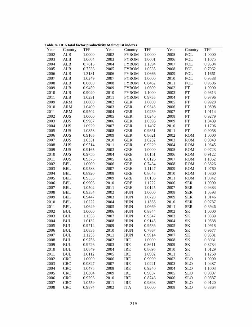
215

Table 36 DEA total factor productivity Malmquist indexes

Year Country TFP Year Country TFP Year Country TFP

2002 ALB 1.0000 2002 FYROM 1.0000 2005 POL 1.0000

2003 ALB 1.0604 2003 FYROM 1.0001 2006 POL 1.1075

2004 ALB 0.7615 2004 FYROM 1.1594 2007 POL 0.9504

2005 ALB 0.7536 2005 FYROM 1.0535 2008 POL 0.7062

2006 ALB 1.3181 2006 FYROM 1.0666 2009 POL 1.1661

2007 ALB 1.0249 2007 FYROM 1.0000 2010 POL 0.9538

2008 ALB 0.6800 2008 FYROM 0.8462 2011 POL 0.9506

2009 ALB 0.9459 2009 FYROM 1.0609 2002 PT 1.0000

2010 ALB 0.9040 2010 FYROM 1.1000 2003 PT 0.9813

2011 ALB 1.0231 2011 FYROM 0.9755 2004 PT 0.9796

2009 ARM 1.0000 2002 GER 1.0000 2005 PT 0.9920

2010 ARM 1.0409 2003 GER 0.9543 2006 PT 1.0808

2011 ARM 0.9502 2004 GER 1.0239 2007 PT 1.0114

2002 AUS 1.0000 2005 GER 1.0240 2008 PT 0.9279

2003 AUS 0.9967 2006 GER 1.0396 2009 PT 1.0489

2004 AUS 1.0929 2007 GER 1.1407 2010 PT 1.1796

2005 AUS 1.0353 2008 GER 0.9851 2011 PT 0.9058

2006 AUS 0.9165 2009 GER 0.8621 2002 ROM 1.0000

2007 AUS 1.0331 2010 GER 1.0232 2003 ROM 0.9049

2008 AUS 0.9514 2011 GER 0.9220 2004 ROM 1.0645

2009 AUS 0.9165 2003 GRE 1.0000 2005 ROM 0.9723

2010 AUS 0.9756 2004 GRE 1.0151 2006 ROM 0.9122

2011 AUS 0.9375 2005 GRE 0.8126 2007 ROM 1.1052

2002 BEL 1.0000 2006 GRE 0.7434 2008 ROM 0.8826

2003 BEL 0.9588 2007 GRE 1.1147 2009 ROM 1.0760

2004 BEL 0.8920 2008 GRE 0.8648 2010 ROM 1.0860

2005 BEL 0.9535 2009 GRE 1.0136 2011 ROM 1.0342

2006 BEL 0.9906 2010 GRE 1.1222 2006 SER 1.0000

2007 BEL 1.0502 2011 GRE 1.0145 2007 SER 0.9383

2008 BEL 0.9354 2002 HUN 1.0000 2008 SER 1.0593

2009 BEL 0.9447 2003 HUN 1.0720 2009 SER 1.0146

2010 BEL 1.0222 2004 HUN 1.1358 2010 SER 0.9737

2011 BEL 1.0649 2005 HUN 1.0669 2011 SER 0.8946

2002 BUL 1.0000 2006 HUN 0.8844 2002 SK 1.0000

2003 BUL 1.1558 2007 HUN 0.9347 2003 SK 1.0339

2004 BUL 1.0132 2008 HUN 0.9145 2004 SK 1.0538

2005 BUL 0.9714 2009 HUN 0.9536 2005 SK 1.0918

2006 BUL 1.0835 2010 HUN 0.7867 2006 SK 0.9677

2007 BUL 1.1253 2011 HUN 0.9914 2007 SK 0.9581

2008 BUL 0.9756 2002 IRE 1.0000 2008 SK 0.8931

2009 BUL 0.9726 2003 IRE 0.8611 2009 SK 0.8734

2010 BUL 1.0849 2004 IRE 0.8695 2010 SK 1.0129

2011 BUL 1.0112 2005 IRE 1.0902 2011 SK 1.1260

2002 CRO 1.0000 2006 IRE 0.9090 2002 SLO 1.0000

2003 CRO 0.9827 2007 IRE 1.0221 2003 SLO 1.0487

2004 CRO 1.0475 2008 IRE 0.9240 2004 SLO 1.1003

2005 CRO 1.0304 2009 IRE 0.9037 2005 SLO 0.9807

2006 CRO 0.9296 2010 IRE 0.8746 2006 SLO 0.9887

2007 CRO 1.0559 2011 IRE 0.9393 2007 SLO 0.9120

2008 CRO 0.9874 2002 ITA 1.0000 2008 SLO 0.8864

216

2009 CRO 0.9943 2003 ITA 0.8422 2009 SLO 0.8798

2010 CRO 0.9934 2004 ITA 0.9226 2010 SLO 0.9394

2011 CRO 0.9605 2005 ITA 0.9929 2011 SLO 0.9449

2002 CYP 1.0000 2006 ITA 1.0555 2002 SP 1.0000

2003 CYP 0.9549 2007 ITA 1.0333 2003 SP 0.8454

2004 CYP 0.7664 2008 ITA 0.9269 2004 SP 0.9190

2005 CYP 0.9594 2009 ITA 0.9254 2005 SP 0.9963

2006 CYP 0.9821 2010 ITA 1.0160 2006 SP 0.9525

2007 CYP 1.0500 2011 ITA 0.9634 2007 SP 0.9490

2008 CYP 1.0598 2002 LAT 1.0000 2008 SP 0.9076

2009 CYP 0.9359 2003 LAT 1.0401 2009 SP 0.9087

2010 CYP 1.0738 2004 LAT 1.5614 2010 SP 1.2639

2011 CYP 1.0996 2005 LAT 0.9696 2011 SP 1.0524

2002 CZ 1.0000 2006 LAT 0.8920 2002 SWE 1.0000

2003 CZ 1.0929 2007 LAT 0.9113 2003 SWE 1.0128

2004 CZ 1.0693 2008 LAT 1.1001 2004 SWE 1.0222

2005 CZ 0.9495 2009 LAT 1.0032 2005 SWE 0.9593

2006 CZ 0.8826 2010 LAT 0.9925 2006 SWE 0.9203

2007 CZ 0.8934 2011 LAT 1.0343 2007 SWE 0.9153

2008 CZ 0.9551 2002 LIT 1.0000 2008 SWE 0.9895

2009 CZ 1.0270 2003 LIT 0.9528 2009 SWE 0.9050

2010 CZ 0.9209 2004 LIT 1.1177 2010 SWE 0.7906

2011 CZ 0.9352 2005 LIT 1.0424 2011 SWE 1.0725

2002 DEN 1.0000 2006 LIT 0.8318 2002 SWI 1.0000

2003 DEN 0.9358 2007 LIT 1.0529 2003 SWI 0.8808

2004 DEN 0.9724 2008 LIT 0.9671 2004 SWI 0.8698

2005 DEN 0.9771 2009 LIT 0.7890 2005 SWI 1.1347

2006 DEN 1.0698 2010 LIT 1.0061 2006 SWI 0.9377

2007 DEN 0.8207 2011 LIT 1.0107 2007 SWI 1.0096

2008 DEN 0.9279 2002 MAL 1.0000 2008 SWI 0.9934

2009 DEN 0.8802 2003 MAL 0.8513 2009 SWI 0.9164

2010 DEN 1.0914 2004 MAL 1.2438 2010 SWI 0.9214

2011 DEN 1.0697 2005 MAL 0.9479 2011 SWI 0.8998

2002 EC 1.0000 2006 MAL 0.9751 2002 TUR 1.0000

2003 EC 0.9626 2007 MAL 0.9869 2003 TUR 0.9338

2004 EC 1.0558 2008 MAL 1.0237 2004 TUR 1.0676

2005 EC 1.0782 2009 MAL 0.9894 2005 TUR 1.1411

2006 EC 1.0248 2010 MAL 1.0293 2006 TUR 0.9899

2007 EC 1.0183 2011 MAL 1.0008 2007 TUR 1.0465

2008 EC 0.9552 2002 MOL 1.0000 2008 TUR 1.0468

2009 EC 0.8682 2003 MOL 0.7862 2009 TUR 1.0296

2010 EC 0.9913 2004 MOL 0.8482 2010 TUR 1.0097

2011 EC 1.1192 2005 MOL 0.8884 2011 TUR 0.9693

2002 EST 1.0000 2006 MOL 0.9704 2002 UK 1.0000

2003 EST 1.0166 2007 MOL 0.8165 2003 UK 0.9268

2004 EST 1.1220 2008 MOL 0.7020 2004 UK 1.0827

2005 EST 1.1139 2009 MOL 0.8835 2005 UK 0.9733

2006 EST 0.9096 2010 MOL 0.9307 2006 UK 1.0281

2007 EST 1.0583 2011 MOL 1.1444 2007 UK 0.9618

2008 EST 0.8213 2002 NL 1.0000 2008 UK 1.1242

2009 EST 1.0233 2003 NL 0.9202 2009 UK 0.9548

2010 EST 0.8136 2004 NL 0.9953 2010 UK 0.9305

2011 EST 0.9944 2005 NL 0.8769 2011 UK 1.0615

217

2002 FIN 1.0000 2006 NL 1.2075 2003 UKR 1.0000

2003 FIN 1.0211 2007 NL 1.0149 2004 UKR 1.2418

2004 FIN 1.0320 2008 NL 0.9416 2005 UKR 0.9334

2005 FIN 0.9799 2009 NL 0.8266 2006 UKR 0.7833

2006 FIN 1.0555 2010 NL 1.1044 2007 UKR 1.0679

2007 FIN 0.9339 2011 NL 1.0412 2008 UKR 0.9939

2008 FIN 0.9883 2002 NOR 1.0000 2009 UKR 0.9982

2009 FIN 0.9069 2003 NOR 1.2547 2010 UKR 0.9214

2010 FIN 0.9865 2004 NOR 1.3134 2011 UKR 0.7212

2011 FIN 1.0216 2005 NOR 0.8643

2002 FRA 1.0000 2006 NOR 0.9073

2003 FRA 0.9392 2007 NOR 0.8279

2004 FRA 0.9838 2008 NOR 1.0640

2005 FRA 0.9926 2009 NOR 1.0149

2006 FRA 1.0215 2010 NOR 0.9186

2007 FRA 0.9430 2011 NOR 0.9874

2008 FRA 0.9609

2009 FRA 0.9103

2010 FRA 1.0063

2011 FRA 1.0217

Key: Albania (ALB), Armenia (ARM), Austria (AUS), Belgium (BEL), Bulgaria (BUL), Croatia (CRO)

Cyprus (CYP), Czech Republic (CZ), Denmark (DEN), EUROCONTROL (EC), Estonia (EST), Finland

(FIN), France (FRA), Republic of Macedonia (FYROM), Germany (GER), Greece (GRE), Hungary

(HUN), Ireland (IRE), Italy (ITA), Latvia (LAT), Lithuania (LIT), Malta (MAL), Moldova (MOL),

Netherlands (NL), Norway (NOR), Poland (POL), Portugal (PT), Romania (ROM), Serbia (SEB), Slovakia

(SK), Slovenia (SLO), Spain (SP), Sweden (SWE), Switzerland (SWI), Turkey (TUR), United Kingdom

(UK), and Ukraine (UKR).

Total Factor Productivity values equal 1 in the first year of the time series for each ANSP – 2002 for most.

218

APPENDIX III – ANSP DEA ANALYSIS: FIGURES

219

220

221

222

Figure 14 DEA efficiency results for each year

Key: Albania (ALB), Armenia (ARM), Austria (AUS), Belgium (BEL), Bulgaria

(BUL), Croatia (CRO) Cyprus (CYP), Czech Republic (CZ), Denmark (DEN),

EUROCONTROL (EC), Estonia (EST), Finland (FIN), France (FRA), Republic of

Macedonia (FYROM), Germany (GER), Greece (GRE), Hungary (HUN), Ireland

(IRE), Italy (ITA), Latvia (LAT), Lithuania (LIT), Malta (MAL), Moldova (MOL),

Netherlands (NL), Norway (NOR), Poland (POL), Portugal (PT), Romania (ROM),

Serbia (SEB), Slovakia (SK), Slovenia (SLO), Spain (SP), Sweden (SWE),

Switzerland (SWI), Turkey (TUR), United Kingdom (UK), and Ukraine (UKR).

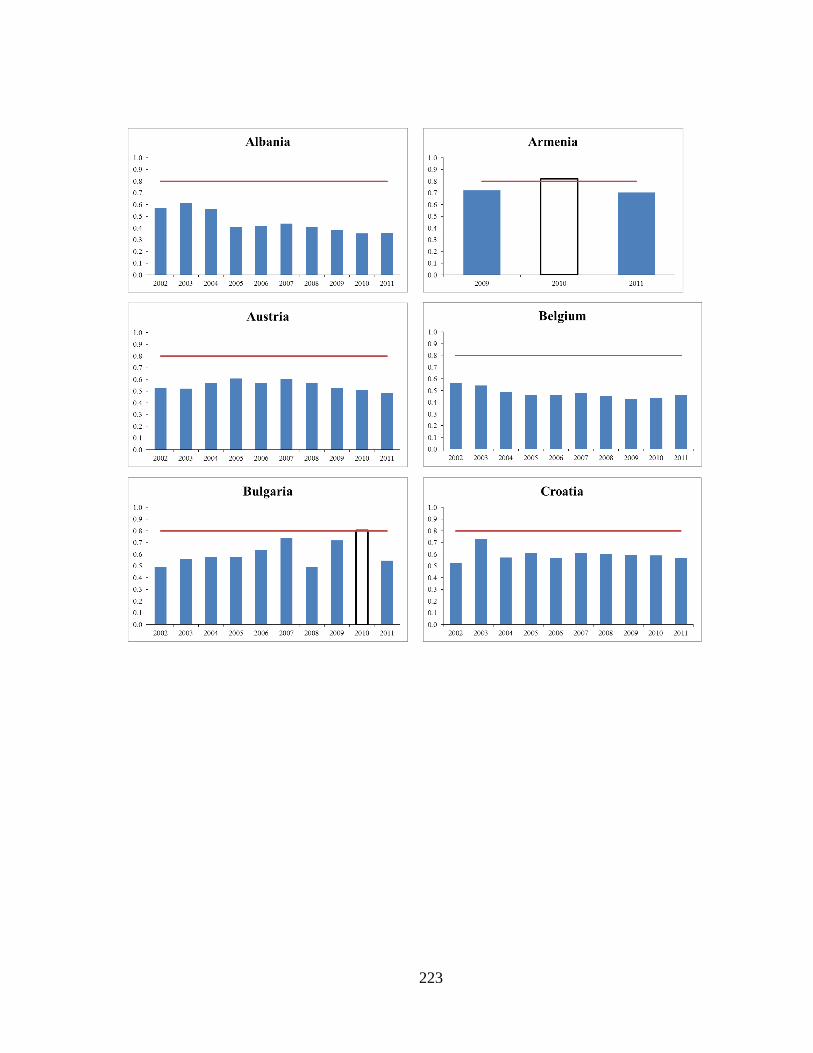
223

224

225

226

227

228

Figure 15 DEA results for each ANSP

229

230

231

232

233

234

Figure 16 DEA total factor productivity Malmquist indexes for each ANSP

235

APPENDIX IV – ANSP DEA ANALYSIS: REGRESSIONS

Table 37 DEA regression with temporal dummy variables

Variable Model

1

2

3

4

(intercept) 6.338e-1***

(14.189)

6.215e-1***

(14.698)

5.681e-1***

(21.263)

6.166e-1***

(14.266)

AGENCY 4.723e-2**

(2.550)

5.231e-2**

(2.927)

7.868e-2***

(4.050)

3.780e-2**

(2.047)

AREA -3.449e-5

(-1.111) -

8.357e-5***

(3.721) -

SECTORS 2.261e-3**

(3.093)

2.931e-3***

(10.278)

1.638e-3***

(4.412) -

ATCO 5.107e-5

(1.257) - -

1.218e-4***

(9.522)

ATCOkm -5.474e-2***

(-7.972)

-5.079e-2***

(-9.049) -

-4.661e-2***

(-8.277)

STAFF_ATCO -9.854e-3*

(-1.796)

-9.693e-3*

(-1.768) -

-1.174e-2**

(-2.116)

REV_COST 8.251e-2**

(2.922)

8.229e-2**

(2.955) -

9.756e-2***

(3.437)

Y2003 4.250e-3

(0.132)

7.289e-3

(0.227)

4.177e-3

(0.117)

-2.873e-3

(-0.088)

Y2004 1.268e-2

(0.394)

1.585e-2

(0.494)

1.783e-2

(0.499)

5.092e-3

(0.156)

Y2005 2.400e-2

(0.750)

2.735e-2

(0.859)

3.004e-2

(0.847)

1.613e-2

(0.498)

Y2006 1.431e-2

(0.451)

1.705e-2

(0.539)

1.864e-2

(0.529)

8.981e-3

(0.279)

Y2007 1.211e-2

(0.382)

1.444e-2

(0.457)

1.424e-2

(0.405)

7.220e-3

(0.224)

Y2008 -2.866e-2

(-0.903)

-2.640e-2

(-0.834)

-2.201e-2

(-0.625)

-3.435e-2

(-1.066)

Y2009 -5.470e-2*

(-1.735)

-5.211e-2*

(-1.658)

-5.283e-2

(-1.510)

-6.125e-2*

(-1.916)

Y2010 -4.572e-2

(-1.447)

-4.275e-2

(-1.359)

-4.136e-2

(-1.182)

-5.332e-2*

(-1.666)

Y2011 -9.248e-2**

(-2.643)

-9.163e-2**

(-2.620)

-4.175e-2

(-1.193)

-9.651e-2**

(-2.715)

Adjusted R-squared 0.3873 0.3878 0.2408 0.3665

Notes ***significant at 0.001; ** significant at 0.05; *significant at 0.1; t-values in parentheses.

Positive signs in the coefficients indicate that the variable is associated with larger levels of efficiency.

236

Table 38 DEA regression with geographical dummy variables

Variable Model

1

2

3

4

(intercept) 20.26***

(5.496)

20.71***

(5.498)

18.71***

(5.653)

20.39***

(5.448)

YEAR -9.902e-3***

(-5.399)

-1.007e-2***

(-5.376)

-9.136e-3***

(-5.537)

-9.914e-3***

(-5.325)

AGENCY -1.266e-2

(-0.361)

-1.621e-2

(-0.452)

-1.357e-2

(-0.389)

-1.509e-2

(-0.423)

AREA 1.347e-3***

(3.607) -

1.436e-3***

(4.045) -

SECTORS -9.655e-4

(-0.929)

-6.110e-4

(-0.577)

-9.566e-4

(-0.923) -

ATCO 8.197e-5

(1.216) - -

1.333e-4**

(1.987)

ATCOkm -1.070e-2

(-0.601)

1.390e-2

(0.893) -

-4.957e-3

(-0.275)

STAFF_ATCO -3.769e-3

(-0.792)

-4.909e-3

(-1.014) -

-3.739e-3

(-0.772)

REV_COST 2.113e-2

(0.868)

1.882e-2

(0.757) -

1.597e-2

(0.645)

ARM 3.131e-1***

(5.092)

2.051e-1***

(3.600)

3.054e-1***

(5.286)

2.340e-1***

(4.042)

AUS 4.761e-2

(0.984)

-7.958e-3

(-0.168)

4.489e-2

(1.304)

9.538e-3

(0.199)

BEL 6.083e-2

(0.721)

-1.061e-1

(-1.430)

2.972e-2

(0.780)

-3.817e-2

(-0.470)

CRO -2.414e-2

(-0.564)

6.785e-2*

(1.853)

-1.834e-2

(-0.440)

5.390e-2

(1.531)

CYP 5.626e-2

(0.904)

1.888e-1***

(3.572)

6.021e-2

(1.060)

1.816e-1***

(3.449)

CZ 6.597e-2*

(1.756)

3.153e-1

(0.780)

6.178e-2*

(1.830)

3.996e-2

(1.064)

DEN 9.383e-2**

(2.221)

1.876e-1***

(5.284)

1.007e-1**

(2.457)

1.779e-1***

(5.026)

EC 6.947e-2

(0.823)

3.153e-1***

(5.563)

9.480e-2

(1.231)

2.906e-1***

(5.182)

EST 3.146e-1***

(8.183)

3.096e-1***

(7.869)

3.325e-1***

(9.857)

3.112e-1***

(7.965)

FIN -1.166e-1

(-0.914)

3.433e-1***

(8.904)

-1.281e-1

(-1.068)

3.210e-1***

(8.045)

FRA -1.007**

(-2.914)

3.577e-1***

(3.466)

-8.954e-1**

(-2.721)

7.754e-3

(0.049)

FYROM -3.057e-2

(-0.567)

-1.477e-1**

(-3.143)

-3.887e-2

(-0.789)

-1.172e-1**

(-2.401)

GER -8.027e-2

(-0.516)

3.359e-1**

(2.832)

-8.196e-3

(-0.057)

1.330e-1

(1.450)

GRE -4.209e-1**

(-2.445)

2.215e-1***

(4.201)

-4.163e-1**

(-2.511)

1.581e-1**

(2.637)

HUN 1.586e-1***

(4.425)

1.479e-1***

(4.052)

1.614e-1***

(4.831)

1.544e-1***

(4.236)

IRE -3.365e-1** 1.795e-1*** -3.411e-1** 1.502e-1***

237

(-2.368) (4.524) (-2.551) (3.704)

ITA -7.620e-1**

(-3.202)

1.672e-1**

(2.569)

-7.206e-1**

(-3.114)

-4.949e-3

(-0.062)

LAT 1.515e-1***

(4.272)

1.658e-1***

(4.591)

1.571e-1***

(4.699)

1.656e-1***

(4.617)

LIT 2.281e-2

(0.660)

6.330e-3

(0.180)

2.852e-2

(0.843)

1.102e-2

(0.316)

MAL -1.667e-1**

(-2.474)

4.039e-2

(1.035)

-1.677e-1**

(-2.794)

3.452e-2

(0.887)

MOL 1.652e-1***

(4.166)

7.978e-2**

(2.317)

1.604e-1***

(4.121)

9.518e-2**

(2.736)

NL 7.844e-2

(1.478)

-2.379e-2

(-0.498)

6.038e-2**

(1.669)

1.025e-2

(0.203)

NOR -6.630e-1**

(-2.811)

2.165e-1***

(5.428)

-6.821e-1**

(-3.037)

1.651e-1***

(3.778)

POL -8.295e-2

(-0.820)

2.701e-1***

(5.687)

-7.594e-2

(-0.779)

2.337e-1***

(4.645)

PT -7.621e-1***

(-3.484)

4.038e-2

(1.055)

-7.904e-1***

(-3.829)

1.205e-2

(0.299)

ROM -8.665e-2

(-1.275)

1.441e-1***

(3.808)

-7.241e-2

(-1.079)

1.040e-1**

(2.581)

SER 8.599e-2*

(1.901)

1.573e-1***

(3.712)

8.981e-2**

(2.016)

1.493e-1***

(3.540)

SK -1.036e-1**

(-2.485)

-1.857e-1***

(-4.946)

-1.080e-1**

(-2.959)

-1.637e-1***

(-4.213)

SLO -1.105e-2

(-0.171)

-1.703e-1**

(-3.252)

-2.423e-2

(-0.573)

-1.141e-1*

(-1.949)

SP -2.744***

(-3.577)

2.125e-1**

(3.071)

-2.777***

(-3.742)

-5.216e-2

(-0.427)

SWE -4.306e-1**

(-2.128)

3.253e-1***

(6.341)

-4.314e-1**

(-2.228)

2.592e-1***

(4.682)

SWI 2.425e-2

(0.402)

-6.070e-2

(-1.050)

1.316e-2

(0.361)

-3.578e-2

(-0.610)

TUR -9.227e-1**

(-2.767)

3.391e-1***

(6.194)

-9.584e-1**

(-3.004)

2.468e-1***

(3.652)

UK -7.791e-1**

(-2.677)

3.503e-1***

(4.383)

-7.422e-1**

(-2.625)

1.509e-1*

(1.736)

UKR -7.950e-1**

(-3.202)

1.800e-1***

(3.932)

-7.787e-1**

(-3.229)

4.227e-2

(0.601)

Adjusted R-squared 0.7312 0.7182 0.7318 0.7214

Notes ***significant at 0.001; ** significant at 0.05; *significant at 0.1; t-values in parentheses.

Key: Armenia (ARM), Austria (AUS), Belgium (BEL), Bulgaria (BUL), Croatia (CRO) Cyprus (CYP),

Czech Republic (CZ), Denmark (DEN), EUROCONTROL (EC), Estonia (EST), Finland (FIN), France

(FRA), Republic of Macedonia (FYROM), Germany (GER), Greece (GRE), Hungary (HUN), Ireland

(IRE), Italy (ITA), Latvia (LAT), Lithuania (LIT), Malta (MAL), Moldova (MOL), Netherlands (NL),

Norway (NOR), Poland (POL), Portugal (PT), Romania (ROM), Serbia (SEB), Slovakia (SK), Slovenia

(SLO), Spain (SP), Sweden (SWE), Switzerland (SWI), Turkey (TUR), United Kingdom (UK), and

Ukraine (UKR). Albania was excluded for identification purposes.

Positive signs in the coefficients indicate that the variable is associated with larger levels of efficiency.

238

Table 39 DEA regression results with COMPLEX variable

Notes ***significant at 0.001; ** significant at 0.05; *significant at 0.1; t-values in parentheses.

Positive signs in the coefficients indicate that the variable is associated with larger levels of efficiency.

Variable Model

1

2

3

4

(intercept) 38.81***

(3.511)

38.58***

(3.483)

27.92**

(2.528)

39.17***

(3.494)

YEAR -1.901e-2***

(-3.457)

-1.891e-2***

(-3.432)

-1.361e-2**

(-2.474)

-1.921e-2***

(-3.443)

AGENCY 5.127e-2**

(2.114)

5.803e-2**

(2.603)

9.476e-2***

(3.944)

4.202e-2*

(1.819)

AREA -6.790e-5*

(-1.719) -

3.503e-5

(1.119) -

SECTORS 1.809e-3

(1.611)

2.381e-3***

(6.271)

2.331e-3***

(4.104) -

ATCO 6.208e-5

(1.050) - -

9.506e-5***

(5.764)

ATCOkm -8.037e-2***

(-6.251)

-6.864e-2***

(-6.334) -

-7.256e-2***

(-6.664)

STAFF_ATCO -2.806e-3

(-0.443)

-2.435e-3

(-0.384) -

-4.070e-3

(-0.638)

REV_COST 4.330e-2

(1.404)

4.973e-2

(1.629) -

5.192e-2*

(1.672)

COMPLEX 1.157e-2**

(2.404)

9.813e-3**

(2.151)

-8.304e-3**

(-2.377)

1.382e-2**

(3.136)

Adjusted R-squared 0.4096 0.4070 0.2562 0.3921

239

Table 40 DEA regression results with DENS and STRUCT variables

Notes ***significant at 0.001; ** significant at 0.05; *significant at 0.1; t-values in parentheses.

Positive signs in the coefficients indicate that the variable is associated with larger levels of efficiency.

Variable Model

1

2

3

4

(intercept) 36.17**

(3.277)

36.51**

(3.290)

26.17**

(2.359)

36.87**

(3.279)

YEAR -1.775e-2**

(-3.233)

-1.793e-2**

(-3.248)

-1.273e-2**

(-2.305)

-1.812e-2**

(-3.240)

AGENCY 5.054e-2**

(2.102)

5.921e-2**

(2.656)

1.006e-1***

(4.149)

4.248e-2*

(1.843)

AREA -8.494e-5**

(-2.126) -

3.518e-5

(1.135) -

SECTORS 1.651e-3

(1.516)

2.429e-3***

(6.427)

2.336e-3***

(4.136) -

ATCO 8.177e-5

(1.386) - -

9.855e-5***

(5.902)

ATCOkm -8.182e-2***

(-6.651)

-6.788e-2***

(-6.485) -

-6.996e-2***

(-6.618)

STAFF_ATCO -5.923e-4

(-0.093)

-5.088e-4

(-0.080) -

-2.022e-3

(-0.314)

REV_COST 5.274e-2*

(1.734)

5.749e-2*

(1.909) -

6.368e-2**

(2.067)

DENS 4.719e-3

(1.006)

4.284e-3

(0.910)

-1.083e-2**

(-2.572)

6.503e-3

(1.390)

STRUCT 1.531e-1**

(3.161)

1.230e1**

(2.694)

1.288e-2

(0.276)

1.506e-1**

(3.294)

Adjusted R-squared 0.4203 0.4133 0.2569 0.3978

240

APPENDIX V – FAB DEA ANALYSIS: TABLES

Table 41 DEA efficiency results – FAB analysis

Year FAB Efficiency Year FAB Efficiency

2005 BALTIC FAB 1.0000 2002 FABEC 1.0000

2006 BALTIC FAB 1.0000 2003 FABEC 0.9496

2007 BALTIC FAB 1.0000 2004 FABEC 0.9506

2008 BALTIC FAB 0.8211 2005 FABEC 0.9589

2009 BALTIC FAB 0.9190 2006 FABEC 1.0000

2010 BALTIC FAB 0.9074 2007 FABEC 1.0000

2011 BALTIC FAB 0.9341 2008 FABEC 1.0000

2003 BLUE MED 0.9539 2009 FABEC 0.8634

2004 BLUE MED 0.8943 2010 FABEC 0.8697

2005 BLUE MED 0.8908 2011 FABEC 0.8447

2006 BLUE MED 0.8709 2002 NEFAB 1.0000

2007 BLUE MED 0.9313 2003 NEFAB 0.9869

2008 BLUE MED 0.9346 2004 NEFAB 1.0000

2009 BLUE MED 0.8887 2005 NEFAB 0.9883

2010 BLUE MED 0.9462 2006 NEFAB 1.0000

2011 BLUE MED 0.9149 2007 NEFAB 0.9085

2002 DANUBE 1.0000 2008 NEFAB 0.8754

2003 DANUBE 1.0000 2009 NEFAB 0.8118

2004 DANUBE 1.0000 2010 NEFAB 0.8401

2005 DANUBE 0.9463 2011 NEFAB 0.8786

2006 DANUBE 0.9074 2002 SW FAB 0.8882

2007 DANUBE 1.0000 2003 SW FAB 0.7710

2008 DANUBE 0.7141 2004 SW FAB 0.7263

2009 DANUBE 1.0000 2005 SW FAB 0.7359

2010 DANUBE 1.0000 2006 SW FAB 0.7204

2011 DANUBE 0.7742 2007 SW FAB 0.6968

2002 DEN-SWE 1.0000 2008 SW FAB 0.6288

2003 DEN-SWE 0.9930 2009 SW FAB 0.5678

2004 DEN-SWE 1.0000 2010 SW FAB 0.7238

2005 DEN-SWE 1.0000 2011 SW FAB 0.7652

2006 DEN-SWE 1.0000 2002 UK-IRE 1.0000

2007 DEN-SWE 0.9400 2003 UK-IRE 0.8630

2008 DEN-SWE 0.9105 2004 UK-IRE 0.9196

2009 DEN-SWE 0.8101 2005 UK-IRE 0.9171

2010 DEN-SWE 0.7324 2006 UK-IRE 0.9386

2011 DEN-SWE 0.7946 2007 UK-IRE 0.9175

2002 FABCE 0.7552 2008 UK-IRE 1.0000

2003 FABCE 0.8039 2009 UK-IRE 0.9278

2004 FABCE 0.9267 2010 UK-IRE 0.8672

2005 FABCE 1.0000 2011 UK-IRE 0.9189

2006 FABCE 0.9283

241

2007 FABCE 0.9292

2008 FABCE 0.8882

2009 FABCE 0.8613

2010 FABCE 0.8209

2011 FABCE 0.7990

242

Table 42 DEA allocative efficiency results – FAB analysis

Year FAB Efficiency Year FAB Efficiency

2005 BALTIC FAB 1.0000 2002 FABEC 1.0000

2006 BALTIC FAB 1.0000 2003 FABEC 0.9951

2007 BALTIC FAB 0.9930 2004 FABEC 0.9767

2008 BALTIC FAB 1.0000 2005 FABEC 0.9953

2009 BALTIC FAB 1.0000 2006 FABEC 0.9824

2010 BALTIC FAB 0.9798 2007 FABEC 0.9628

2011 BALTIC FAB 1.0000 2008 FABEC 0.9942

2003 BLUE MED 0.9581 2009 FABEC 0.9857

2004 BLUE MED 0.9972 2010 FABEC 0.9787

2005 BLUE MED 0.9843 2011 FABEC 1.0000

2006 BLUE MED 0.9807 2002 NEFAB 0.9937

2007 BLUE MED 0.9857 2003 NEFAB 0.9775

2008 BLUE MED 0.9855 2004 NEFAB 1.0000

2009 BLUE MED 0.9782 2005 NEFAB 0.9833

2010 BLUE MED 0.9913 2006 NEFAB 0.9640

2011 BLUE MED 0.9606 2007 NEFAB 1.0000

2002 DANUBE 1.0000 2008 NEFAB 0.9682

2003 DANUBE 0.9797 2009 NEFAB 0.9828

2004 DANUBE 0.9746 2010 NEFAB 0.9992

2005 DANUBE 0.9785 2011 NEFAB 0.9778

2006 DANUBE 0.9995 2002 SW FAB 0.9766

2007 DANUBE 0.9780 2003 SW FAB 0.9987

2008 DANUBE 0.9945 2004 SW FAB 0.9864

2009 DANUBE 1.0000 2005 SW FAB 0.9627

2010 DANUBE 0.9622 2006 SW FAB 1.0000

2011 DANUBE 0.9980 2007 SW FAB 0.9586

2002 DEN-SWE 1.0000 2008 SW FAB 0.9845

2003 DEN-SWE 0.9706 2009 SW FAB 0.9952

2004 DEN-SWE 0.9792 2010 SW FAB 0.9695

2005 DEN-SWE 0.9962 2011 SW FAB 0.9681

2006 DEN-SWE 0.9734 2002 UK-IRE 0.9973

2007 DEN-SWE 0.9951 2003 UK-IRE 0.9764

2008 DEN-SWE 1.0000 2004 UK-IRE 0.9663

2009 DEN-SWE 0.9630 2005 UK-IRE 0.9916

2010 DEN-SWE 1.0000 2006 UK-IRE 0.9500

2011 DEN-SWE 1.0000 2007 UK-IRE 0.9852

2002 FABCE 0.9755 2008 UK-IRE 0.9931

2003 FABCE 0.9823 2009 UK-IRE 0.9616

2004 FABCE 1.0000 2010 UK-IRE 0.9597

2005 FABCE 0.9721 2011 UK-IRE 0.9985

2006 FABCE 0.9972

2007 FABCE 0.9845

2008 FABCE 0.9586

2009 FABCE 1.0000

2010 FABCE 0.9886

2011 FABCE 0.9793

243

Table 43 DEA inputs and outputs slacks – FAB analysis

Year FAB

Slacks

Provision

costs

Other

costs

IFR flight

hours

Airport

movements 1/delays

2005 BALTIC FAB 0.0000 0.0000 0.0000 0.0000 0.0000

2006 BALTIC FAB 0.0000 0.0000 0.0000 0.0000 0.0000

2007 BALTIC FAB 1.7425 0.0000 0.0000 281.0310 0.0000

2008 BALTIC FAB 0.0000 0.0000 0.0000 0.0000 0.0000

2009 BALTIC FAB 0.0000 0.0000 0.0000 0.0000 0.0000

2010 BALTIC FAB 0.0000 0.0000 0.0000 0.0000 0.0029

2011 BALTIC FAB 0.0000 0.0000 0.0000 0.0000 0.0000

2003 BLUE MED 0.0000 0.0000 0.0000 0.0000 0.0012

2004 BLUE MED 0.0000 0.0000 0.0000 0.0000 0.0000

2005 BLUE MED 0.0000 0.0000 0.0000 0.0000 0.0000

2006 BLUE MED 4.6902 0.0000 0.0000 222.9706 0.0000

2007 BLUE MED 35.7290 0.0000 0.0000 0.0000 0.0000

2008 BLUE MED 0.0000 0.0000 18.7615 0.0000 0.0000

2009 BLUE MED 0.0000 0.0000 0.0000 0.0000 0.0018

2010 BLUE MED 0.0000 12.5064 0.0000 0.0000 0.0016

2011 BLUE MED 0.0000 0.0000 0.0000 0.0000 0.0012

2002 DANUBE 0.0000 0.0000 0.0000 0.0000 0.0000

2003 DANUBE 0.0000 0.0000 0.0000 0.0000 0.0000

2004 DANUBE 2.0485 0.0000 0.0000 93.2697 0.0009

2005 DANUBE 39.1011 0.0000 0.0000 0.0000 0.0000

2006 DANUBE 0.0000 0.0000 0.0000 0.0000 0.0000

2007 DANUBE 0.0000 0.0000 0.0000 0.0000 0.0023

2008 DANUBE 0.0000 8.2255 0.0000 0.0000 0.0011

2009 DANUBE 0.0000 0.0000 0.0000 0.0000 0.0000

2010 DANUBE 0.0000 0.0000 0.0000 0.0000 0.0003

2011 DANUBE 0.0000 0.0928 0.0000 21.1356 0.0000

2002 DEN-SWE 0.0000 0.0000 0.0000 0.0000 0.0000

2003 DEN-SWE 0.0000 0.0000 0.0000 0.0000 0.0000

2004 DEN-SWE 32.0780 0.0000 0.0000 0.0000 0.0000

2005 DEN-SWE 0.0000 0.0000 4.5507 0.0000 0.0000

2006 DEN-SWE 0.0000 0.0000 0.0000 0.0000 0.0025

2007 DEN-SWE 0.0000 7.8400 0.0000 0.0000 0.0005

2008 DEN-SWE 0.0000 0.0000 0.0000 0.0000 0.0000

2009 DEN-SWE 0.0000 0.0000 0.0000 0.0000 0.0002

2010 DEN-SWE 0.0000 0.0000 0.0000 0.0000 0.0000

2011 DEN-SWE 0.0000 0.0000 0.0000 0.0000 0.0000

2002 FABCE 0.0000 0.0000 0.0000 61.7062 0.0001

2003 FABCE 0.0000 0.0000 0.0000 0.0000 0.0000

2004 FABCE 0.0000 0.0000 0.0000 0.0000 0.0000

2005 FABCE 0.0000 0.0000 0.0000 0.0000 0.0023

2006 FABCE 0.0000 4.6986 0.0000 0.0000 0.0001

2007 FABCE 0.0000 0.0000 0.0000 0.0000 0.0000

2008 FABCE 0.0000 0.0000 0.0000 0.0000 0.0003

2009 FABCE 0.0000 0.0000 0.0000 0.0000 0.0000

2010 FABCE 0.0000 5.6653 0.0000 24.6622 0.0011

2011 FABCE 0.0000 0.0000 0.0000 121.1473 0.0002

2002 FABEC 0.0000 0.0000 0.0000 0.0000 0.0000

2003 FABEC 0.0000 0.0000 0.0000 0.0000 0.0000

2004 FABEC 0.0000 0.0000 0.0000 0.0000 0.0017

244

2005 FABEC 0.0000 8.2982 0.0000 0.0000 0.0000

2006 FABEC 0.0000 4.0269 0.0000 106.6608 0.0032

2007 FABEC 0.0000 0.0000 0.0000 355.8995 0.0001

2008 FABEC 0.0000 1.5627 0.0000 162.7372 0.0000

2009 FABEC 0.0000 7.3642 0.0000 8.8936 0.0032

2010 FABEC 0.0000 0.0000 0.0000 122.1182 0.0001

2011 FABEC 0.0000 0.0000 0.0000 0.0000 0.0000

2002 NEFAB 0.0000 0.0000 0.0000 0.0000 0.0043

2003 NEFAB 0.0000 0.0000 0.0000 0.0000 0.0014

2004 NEFAB 0.0000 0.0000 0.0000 0.0000 0.0000

2005 NEFAB 0.0000 3.2160 0.0000 90.5731 0.0028

2006 NEFAB 0.0000 0.0000 0.0000 348.3823 0.0000

2007 NEFAB 0.0000 0.0000 0.0000 0.0000 0.0000

2008 NEFAB 0.0000 14.4454 0.0000 0.0000 0.0000

2009 NEFAB 0.0000 0.0000 0.0000 236.3380 0.0003

2010 NEFAB 0.0000 4.0028 0.0000 34.6421 0.0000

2011 NEFAB 0.0000 0.0000 0.0000 0.0000 0.0000

2002 SW FAB 0.0000 0.0000 0.0000 0.0000 0.0023

2003 SW FAB 0.0000 1.9360 0.0000 0.0622 0.0000

2004 SW FAB 0.0000 2.7750 0.0000 127.3158 0.0027

2005 SW FAB 0.0000 0.0000 0.0000 433.5980 0.0000

2006 SW FAB 0.0000 0.0000 0.0000 0.0000 0.0000

2007 SW FAB 0.0000 19.5944 0.0000 6.2657 0.0000

2008 SW FAB 0.0000 0.0000 0.0000 305.8911 0.0007

2009 SW FAB 0.0000 0.0000 0.0000 15.5337 0.0001

2010 SW FAB 0.0000 2.0968 0.0000 0.0000 0.0000

2011 SW FAB 2.5684 0.0000 0.0000 0.0000 0.0032

2002 UK-IRE 0.0000 3.9376 0.0000 45.2207 0.0004

2003 UK-IRE 0.0000 6.7424 0.0000 188.7661 0.0019

2004 UK-IRE 0.0000 0.0000 0.0000 452.5067 0.0001

2005 UK-IRE 0.0000 2.3935 0.0000 345.2111 0.0000

2006 UK-IRE 0.0000 25.7826 0.0000 18.0513 0.0000

2007 UK-IRE 0.0000 0.0000 0.0000 353.5449 0.0000

2008 UK-IRE 0.0000 35.0437 286.4737 0.0000 0.0000

2009 UK-IRE 0.0000 7.7741 0.0000 0.0000 0.0017

2010 UK-IRE 45.5730 0.0000 0.0000 0.0000 0.0009

2011 UK-IRE 0.0000 2.1951 0.0000 69.0675 0.0000

245

APPENDIX VI – FAB DEA ANALYSIS: FIGURES

246

Figure 17 DEA FAB results for each year

247

248

Figure 18 DEA results for each FAB

249

APPENDIX VII – FAB DEA ANALYSIS: REGRESSIONS

Table 44 FAB regression results with temporal dummy variables

Variable

Model

1

2

3

4

(intercept) 8.253e-1***

(7.687)

4.921e-1***

(4.557)

9.484e-1***

(32.77)

5.109e-1***

(4.696)

AREA -1.289e-4***

(-5.917) -

-6.958-5***

(-6.289)

-

SECTORS -8.595e-4

(-1.300)

-1.697e-4

(-0.717)

4.186e-4**

(3.259)

-

ATCO 1.030e-4**

(2.735) - -

-1.231e-5

(-1.126)

ATCOkm -7.893e-2**

(-2.956)

1.526e-2

(0.597) -

2.357e-2

(0.937)

STAFF_ATCO -2.323e-3

(-0.131)

1.493e-2

(0.706) -

8.349e-3

(0.389)

REV_COST 2.624e-1**

(2.483)

3.608e-1**

(2.970) -

3.572e-1**

(3.047)

Y2003 -2.449e-2

(-0.714)

-9.566e-3

(-0.237)

-2.450e-3

(-0.068)

-6.984e-3

(-0.175)

Y2004 -1.441e-2

(-0.419)

-1.129e-3

(-0.028)

1.047e-2

(0.290)

1.220e-3

(0.030)

Y2005 -2.556e-2

(-0.738)

-7.359e-3

(-0.184)

1.110e-2

(0.316)

-5.018e-3

(-0.128)

Y2006 -2.864e-2

(-0.854)

-1.211e-2

(-0.307)

-2.759e-5

(-0.001)

-1.002e-2

(-0.257)

Y2007 -3.616e-2

(-1.086)

-2.038-2

(-0.519)

-1.070e-2

(-0.305)

-1.816e-2

(-0.466)

Y2008 -9.244e-2**

(-2.753)

-7.778e-2*

(-1.979)

-6.283e-2*

(-1.789)

-7.487e-2*

(-1.918)

Y2009 -8.900e-2**

(-2.670)

-6.636e-2*

(-1.688)

-7.462e-2**

(-2.124)

-6.380e-2

(-1.631)

Y2010 -9.924-e2**

(-2.924)

-8.318e-2**

(-2.112)

-6.679e-2*

(-1.901)

-8.018e-2**

(-2.053)

Y2011 -1.153e-1**

(-3.251)

-1.016e-1**

(-2.487)

-7.016e-2**

(-1.998)

-9.908e-2**

(-2.469)

Adjusted R-squared 0.4762 0.2156 0.3676 0.2237

Notes ***significant at 0.001; ** significant at 0.05; *significant at 0.1; t-values in parentheses.

Positive signs in the coefficients indicate that the variable is associated with larger levels of efficiency.

250

Table 45 FAB regression results with geographical dummy variables

Variable

Model

1

2

3

4

(intercept) 24.51***

(5.559)

25.69***

(5.695)

23.85***

(5.262)

25.66***

(5.723)

YEAR -1.240e-2***

(-5.690)

-1.258e-2***

(-5.564)

-1.147e-2***

(-5.078)

-1.257e-2***

(-5.593)

AREA 5.219e-4**

(2.524) -

7.511e-5*

(1.967)

-

SECTORS -1.728e-3**

(-2.331)

5.304e-5

(0.259)

-3.328e-4

(-1.334)

-

ATCO -1.344e-4

(-1.422) - -

8.329e-6

(0.818)

ATCOkm 3.161e-1**

(2.328)

1.060e-2

(0.432) -

-2.172e-3

(-0.081)

STAFF_ATCO 3.670e-2

(1.060)

1.551e-2

(0.436) -

2.492e-2

(0.688)

REV_COST 3.915e-1**

(3.358)

3.361e-1**

(2.750) -

3.250e-1**

(2.676)

BALTIC 2.309e-1**

(2.227)

2.889e-2

(0.891)

5.760e-2*

(1.973)

2.445e-2

(0.746)

BLUEMED -4.167e-2

(-0.705)

8.171e-2*

(1.704)

-2.580e-2

(-0.699)

8.092e-2*

(1.703)

DEN_SWE 5.487e-2

(1.322)

1.558e-2

(0.526)

2.650e-2

(1.004)

1.619e-2

(0.561)

FABCE 2.353e-1**

(2.642)

5.580e-2

(1.028)

-1.364e-3

(-0.055)

6.164e-2

(1.144)

SWFAB 2.891e-1**

(2.818)

8.156e-2*

(1.906)

1.339e-2

(0.522)

7.820e-2*

(1.826)

UK_IRE -6.848e-1**

(-3.127)

-9.246e-2

(-1.490)

-3.167e-1***

(-4.026)

-9.823e-2

(-1.581)

Adjusted R-squared 0.6211 0.5715 0.5571 0.5749

Notes ***significant at 0.001; ** significant at 0.05; *significant at 0.1; t-values in parentheses.

Positive signs in the coefficients indicate that the variable is associated with larger levels of efficiency.

251

APPENDIX VIII – ANSP SFA ANALYSIS: TABLES

Table 46 SFA efficiencies for Cobb-Douglas specifications

Year Country Model

1 2 3 4 Average

2002 ALB 0.3834 0.3037 0.2151 0.2221 0.2811

2003 ALB 0.3642 0.4351 0.2899 0.3130 0.3506

2004 ALB 0.4624 0.4902 0.3229 0.3536 0.4073

2005 ALB 0.4192 0.4648 0.3104 0.3358 0.3826

2006 ALB 0.4251 0.4774 0.3167 0.3429 0.3905

2007 ALB 0.4231 0.5595 0.3661 0.4031 0.4380

2008 ALB 0.5250 0.5150 0.3442 0.3764 0.4402

2009 ALB 0.4887 0.4644 0.3240 0.3439 0.4052

2010 ALB 0.4285 0.3856 0.2871 0.2954 0.3492

2011 ALB 0.5141 0.4406 0.3023 0.3195 0.3941

2009 ARM 0.3034 0.3203 0.2014 0.2333 0.2646

2010 ARM 0.3132 0.3963 0.2415 0.2881 0.3098

2011 ARM 0.4110 0.4414 0.2470 0.3014 0.3502

2002 AUS 0.6058 0.4166 0.4333 0.3888 0.4611

2003 AUS 0.5846 0.4850 0.4903 0.4532 0.5033

2004 AUS 0.7978 0.5916 0.5830 0.5484 0.6302

2005 AUS 0.8007 0.6302 0.6195 0.5879 0.6596

2006 AUS 0.9296 0.5884 0.5934 0.5521 0.6659

2007 AUS 0.9224 0.6842 0.6750 0.6439 0.7314

2008 AUS 0.8853 0.6950 0.6859 0.6607 0.7317

2009 AUS 0.7508 0.6214 0.6179 0.5869 0.6443

2010 AUS 0.6780 0.5858 0.5879 0.5551 0.6017

2011 AUS 0.6533 0.6148 0.5980 0.5717 0.6094

2002 BEL 0.4279 0.2695 0.2951 0.2623 0.3137

2003 BEL 0.4393 0.3211 0.3409 0.3119 0.3533

2004 BEL 0.5171 0.3437 0.3590 0.3319 0.3879

2005 BEL 0.5263 0.3349 0.3486 0.3201 0.3825

2006 BEL 0.5176 0.3351 0.3516 0.3203 0.3812

2007 BEL 0.5223 0.3843 0.3934 0.3680 0.4170

2008 BEL 0.5316 0.4146 0.4184 0.3969 0.4404

2009 BEL 0.5245 0.3612 0.3716 0.3467 0.4010

2010 BEL 0.5236 0.3558 0.3670 0.3408 0.3968

2011 BEL 0.7062 0.4176 0.4015 0.3825 0.4769

2002 BUL 0.3734 0.1344 0.1598 0.1212 0.1972

2003 BUL 0.3913 0.1762 0.1956 0.1569 0.2300

2004 BUL 0.4036 0.2059 0.2225 0.1832 0.2538

2005 BUL 0.4360 0.2177 0.2362 0.1952 0.2713

2006 BUL 0.4839 0.2509 0.2659 0.2249 0.3064

2007 BUL 0.5452 0.3238 0.3280 0.2897 0.3717

2008 BUL 0.5140 0.3750 0.3705 0.3361 0.3989

2009 BUL 0.5195 0.3627 0.3608 0.3253 0.3921

252

2010 BUL 0.5977 0.3725 0.3710 0.3372 0.4196

2011 BUL 0.8825 0.4473 0.4051 0.3817 0.5292

2002 CRO 0.9988 0.3176 0.3268 0.2446 0.4720

2003 CRO 0.7830 0.3378 0.2998 0.2870 0.4269

2004 CRO 0.8098 0.4035 0.3541 0.3435 0.4777

2005 CRO 0.7897 0.4440 0.3918 0.3811 0.5016

2006 CRO 0.7983 0.4448 0.3926 0.3797 0.5039

2007 CRO 0.7376 0.5169 0.4503 0.4433 0.5370

2008 CRO 0.7738 0.5709 0.4926 0.4899 0.5818

2009 CRO 0.7487 0.5462 0.4707 0.4668 0.5581

2010 CRO 0.7809 0.5477 0.4776 0.4698 0.5690

2011 CRO 0.9577 0.5639 0.4797 0.4717 0.6182

2002 CYP 0.9629 0.8221 0.6255 0.6719 0.7706

2003 CYP 0.9596 0.8574 0.6737 0.7389 0.8074

2004 CYP 0.9277 0.7884 0.5972 0.6382 0.7379

2005 CYP 0.9394 0.8467 0.6548 0.7059 0.7867

2006 CYP 0.9094 0.8585 0.6767 0.7318 0.7941

2007 CYP 0.9045 0.8227 0.6456 0.6867 0.7649

2008 CYP 0.9328 0.9187 0.8166 0.9160 0.8960

2009 CYP 0.8895 0.8922 0.7522 0.8216 0.8389

2010 CYP 0.8451 0.9102 0.7984 0.8835 0.8593

2011 CYP 0.8218 0.9084 0.7808 0.8727 0.8459

2002 CZ 0.4746 0.3466 0.3274 0.2982 0.3617

2003 CZ 0.5015 0.4042 0.3787 0.3518 0.4091

2004 CZ 0.5814 0.4819 0.4510 0.4238 0.4845

2005 CZ 0.5722 0.4602 0.4408 0.4114 0.4711

2006 CZ 0.5476 0.4184 0.4116 0.3778 0.4389

2007 CZ 0.5978 0.4252 0.4203 0.3847 0.4570

2008 CZ 0.6062 0.5352 0.5080 0.4801 0.5324

2009 CZ 0.5911 0.4967 0.4782 0.4470 0.5032

2010 CZ 0.6907 0.4807 0.4687 0.4352 0.5188

2011 CZ 0.5407 0.5078 0.4702 0.4457 0.4911

2002 DEN 0.9838 0.7687 0.6858 0.6889 0.7818

2003 DEN 0.8944 0.8539 0.7696 0.8199 0.8345

2004 DEN 0.9086 0.8888 0.8187 0.8929 0.8773

2005 DEN 0.8920 0.8790 0.8012 0.8714 0.8609

2006 DEN 0.8971 0.8939 0.8274 0.9112 0.8824

2007 DEN 0.7163 0.8765 0.8010 0.8733 0.8168

2008 DEN 0.8912 0.8774 0.8041 0.8754 0.8620

2009 DEN 0.8372 0.8176 0.7243 0.7532 0.7831

2010 DEN 0.8735 0.8230 0.7324 0.7657 0.7986

2011 DEN 0.8819 0.8678 0.7813 0.8389 0.8425

2002 EC 0.9921 0.7044 0.5554 0.5823 0.7085

2003 EC 0.9920 0.8033 0.6368 0.6847 0.7792

2004 EC 0.9928 0.8606 0.7105 0.7778 0.8354

2005 EC 0.9929 0.8834 0.7508 0.8352 0.8656

2006 EC 0.9928 0.8900 0.7679 0.8563 0.8767

2007 EC 0.9926 0.9106 0.8106 0.9162 0.9075

2008 EC 0.9958 0.9238 0.8218 0.9376 0.9197

2009 EC 0.9960 0.8909 0.7423 0.8421 0.8678

2010 EC 0.9957 0.8741 0.7185 0.8043 0.8481

2011 EC 0.9905 0.9179 0.8020 0.9244 0.9087

2002 EST 0.6031 0.5907 0.3496 0.4145 0.4895

253

2003 EST 0.7087 0.6686 0.3939 0.4737 0.5612

2004 EST 0.8624 0.8033 0.4750 0.5926 0.6833

2005 EST 0.9463 0.8462 0.5173 0.6528 0.7407

2006 EST 0.9351 0.8676 0.5521 0.6995 0.7636

2007 EST 0.9421 0.9130 0.6416 0.8332 0.8325

2008 EST 0.9033 0.9275 0.6948 0.8998 0.8563

2009 EST 0.8357 0.8925 0.5971 0.7665 0.7730

2010 EST 0.7633 0.8651 0.5602 0.7072 0.7240

2011 EST 0.7485 0.9074 0.6272 0.8080 0.7728

2002 FIN 0.9917 0.6546 0.5560 0.5473 0.6874

2003 FIN 0.9927 0.8080 0.6778 0.7014 0.7950

2004 FIN 0.9930 0.8476 0.7246 0.7643 0.8324

2005 FIN 0.9933 0.8370 0.7125 0.7473 0.8225

2006 FIN 0.9932 0.8447 0.7220 0.7605 0.8301

2007 FIN 0.9935 0.8345 0.7074 0.7465 0.8205

2008 FIN 0.9935 0.8633 0.7425 0.7998 0.8498

2009 FIN 0.9935 0.7963 0.6617 0.6908 0.7856

2010 FIN 0.9934 0.7972 0.6634 0.6894 0.7859

2011 FIN 0.9950 0.8620 0.7431 0.7936 0.8484

2002 FRA 0.9933 0.6916 0.9272 0.6986 0.8277

2003 FRA 0.9937 0.8050 0.9458 0.8369 0.8953

2004 FRA 0.9921 0.8519 0.9526 0.9090 0.9264

2005 FRA 0.9909 0.8470 0.9525 0.9011 0.9229

2006 FRA 0.9877 0.8542 0.9539 0.9145 0.9276

2007 FRA 0.9870 0.8710 0.9570 0.9364 0.9378

2008 FRA 0.9891 0.8782 0.9581 0.9448 0.9426

2009 FRA 0.9588 0.8258 0.9490 0.8761 0.9024

2010 FRA 0.8804 0.8096 0.9463 0.8539 0.8725

2011 FRA 0.9979 0.8657 0.9539 0.9068 0.9311

2002 FYROM 0.2715 0.1805 0.1375 0.1318 0.1804

2003 FYROM 0.2735 0.2163 0.1621 0.1587 0.2027

2004 FYROM 0.2758 0.2571 0.1879 0.1882 0.2272

2005 FYROM 0.2779 0.2236 0.1713 0.1693 0.2105

2006 FYROM 0.2968 0.2288 0.1742 0.1739 0.2184

2007 FYROM 0.3346 0.2420 0.1794 0.1825 0.2346

2008 FYROM 0.3146 0.2218 0.1678 0.1701 0.2186

2009 FYROM 0.2747 0.2039 0.1597 0.1589 0.1993

2010 FYROM 0.4070 0.2050 0.1574 0.1603 0.2325

2011 FYROM 0.4436 0.2358 0.1625 0.1720 0.2535

2002 GER 0.9981 0.5768 0.8638 0.5612 0.7500

2003 GER 0.9981 0.6532 0.8964 0.6359 0.7959

2004 GER 0.9979 0.7296 0.9181 0.7176 0.8408

2005 GER 0.9973 0.7243 0.9165 0.7180 0.8390

2006 GER 0.9980 0.7492 0.9264 0.7366 0.8525

2007 GER 0.9980 0.8140 0.9227 0.7796 0.8786

2008 GER 0.9972 0.8435 0.9396 0.8781 0.9146

2009 GER 0.9975 0.7649 0.9232 0.7531 0.8597

2010 GER 0.9978 0.7311 0.9175 0.7161 0.8406

2011 GER 0.9986 0.7550 0.8985 0.6835 0.8339

2003 GRE 0.9861 0.7192 0.7369 0.6664 0.7771

2004 GRE 0.9868 0.8123 0.8160 0.7785 0.8484

2005 GRE 0.9845 0.7313 0.7516 0.6802 0.7869

2006 GRE 0.9905 0.5548 0.6183 0.5250 0.6721

254

2007 GRE 0.9911 0.6878 0.7363 0.6636 0.7697

2008 GRE 0.9902 0.7142 0.7523 0.6798 0.7841

2009 GRE 0.9902 0.7003 0.7405 0.6670 0.7745

2010 GRE 0.9907 0.7635 0.7890 0.7309 0.8185

2011 GRE 0.9933 0.8366 0.8232 0.8025 0.8639

2002 HUN 0.4291 0.3425 0.3250 0.2953 0.3480

2003 HUN 0.4852 0.4171 0.3846 0.3614 0.4121

2004 HUN 0.5094 0.5821 0.5132 0.5031 0.5269

2005 HUN 0.5170 0.6111 0.5422 0.5364 0.5517

2006 HUN 0.6042 0.5638 0.5109 0.4942 0.5433

2007 HUN 0.6252 0.6610 0.5797 0.5766 0.6106

2008 HUN 0.6197 0.6667 0.5825 0.5810 0.6125

2009 HUN 0.6153 0.5602 0.5071 0.4907 0.5433

2010 HUN 0.5758 0.5470 0.4970 0.4813 0.5253

2011 HUN 0.6502 0.5129 0.4524 0.4368 0.5131

2002 IRE 0.9966 0.7490 0.6785 0.6454 0.7674

2003 IRE 0.9960 0.7790 0.6969 0.6848 0.7892

2004 IRE 0.9961 0.8292 0.7491 0.7427 0.8293

2005 IRE 0.9962 0.8911 0.8373 0.8787 0.9008

2006 IRE 0.9964 0.8622 0.8071 0.8159 0.8704

2007 IRE 0.9964 0.8912 0.8477 0.8893 0.9061

2008 IRE 0.9964 0.9010 0.8598 0.9118 0.9173

2009 IRE 0.9964 0.8543 0.7975 0.7984 0.8616

2010 IRE 0.9962 0.7602 0.7040 0.6673 0.7819

2011 IRE 0.9958 0.7831 0.7143 0.6821 0.7938

2002 ITA 0.9944 0.5961 0.8199 0.5817 0.7480

2003 ITA 0.9941 0.6862 0.8695 0.6640 0.8035

2004 ITA 0.9959 0.7122 0.8804 0.6868 0.8188

2005 ITA 0.9967 0.7704 0.8996 0.7450 0.8529

2006 ITA 0.9974 0.7842 0.9059 0.7626 0.8625

2007 ITA 0.9975 0.8253 0.9201 0.8270 0.8925

2008 ITA 0.9979 0.8416 0.9272 0.8477 0.9036

2009 ITA 0.9977 0.7814 0.9074 0.7542 0.8602

2010 ITA 0.9973 0.7882 0.9108 0.7679 0.8660

2011 ITA 0.9981 0.8147 0.9147 0.7889 0.8791

2002 LAT 0.6431 0.3565 0.2439 0.2521 0.3739

2003 LAT 0.6696 0.4741 0.3101 0.3328 0.4467

2004 LAT 0.8326 0.5371 0.3521 0.3961 0.5294

2005 LAT 0.7708 0.5670 0.3882 0.4343 0.5401

2006 LAT 0.6544 0.5783 0.4021 0.4472 0.5205

2007 LAT 0.5975 0.7271 0.5125 0.5782 0.6038

2008 LAT 0.5945 0.8565 0.6344 0.7415 0.7067

2009 LAT 0.6131 0.8115 0.5715 0.6589 0.6637

2010 LAT 0.5675 0.7361 0.5172 0.5831 0.6010

2011 LAT 0.6518 0.8523 0.6145 0.7157 0.7086

2002 LIT 0.3968 0.2385 0.1598 0.1711 0.2415

2003 LIT 0.4048 0.2530 0.1842 0.1894 0.2579

2004 LIT 0.4841 0.3153 0.2247 0.2382 0.3156

2005 LIT 0.4762 0.3619 0.2568 0.2744 0.3423

2006 LIT 0.4356 0.3807 0.2754 0.2915 0.3458

2007 LIT 0.4972 0.4834 0.3414 0.3717 0.4234

2008 LIT 0.4990 0.6105 0.4174 0.4803 0.5018

2009 LIT 0.4149 0.4396 0.3130 0.3429 0.3776

255

2010 LIT 0.4167 0.4559 0.3283 0.3561 0.3892

2011 LIT 0.6656 0.5487 0.3766 0.4156 0.5016

2002 MAL 0.9815 0.3444 0.2457 0.2595 0.4578

2003 MAL 0.9817 0.4737 0.3229 0.3468 0.5313

2004 MAL 0.9816 0.5419 0.3553 0.3959 0.5687

2005 MAL 0.9842 0.5746 0.3732 0.4182 0.5875

2006 MAL 0.9842 0.5708 0.3711 0.4152 0.5853

2007 MAL 0.9858 0.6134 0.4005 0.4517 0.6128

2008 MAL 0.9863 0.7803 0.4996 0.5837 0.7125

2009 MAL 0.9851 0.7407 0.4724 0.5445 0.6857

2010 MAL 0.9852 0.7821 0.4980 0.5827 0.7120

2011 MAL 0.9843 0.8497 0.5600 0.6666 0.7652

2002 MOL 0.3280 0.1747 0.1110 0.1179 0.1829

2003 MOL 0.3130 0.1725 0.1138 0.1214 0.1802

2004 MOL 0.3321 0.2337 0.1456 0.1620 0.2183

2005 MOL 0.3414 0.2660 0.1660 0.1862 0.2399

2006 MOL 0.3431 0.2794 0.1715 0.1955 0.2474

2007 MOL 0.3571 0.3584 0.2163 0.2507 0.2956

2008 MOL 0.4013 0.4081 0.2440 0.2885 0.3355

2009 MOL 0.3602 0.3668 0.2268 0.2619 0.3039

2010 MOL 0.3664 0.4427 0.2727 0.3166 0.3496

2011 MOL 0.4639 0.5499 0.3069 0.3738 0.4236

2002 NL 0.4479 0.3353 0.3675 0.3213 0.3680

2003 NL 0.3932 0.4046 0.4222 0.3854 0.4014

2004 NL 0.3988 0.4269 0.4401 0.4068 0.4182

2005 NL 0.3581 0.3878 0.4026 0.3699 0.3796

2006 NL 0.4295 0.4212 0.4356 0.4033 0.4224

2007 NL 0.4236 0.4562 0.4649 0.4365 0.4453

2008 NL 0.4220 0.4730 0.4780 0.4505 0.4559

2009 NL 0.4185 0.3785 0.3946 0.3646 0.3890

2010 NL 0.3981 0.4104 0.4197 0.3906 0.4047

2011 NL 0.4988 0.4726 0.4602 0.4386 0.4676

2002 NOR 0.9977 0.6891 0.6881 0.5957 0.7427

2003 NOR 0.9977 0.8794 0.8631 0.8658 0.9015

2004 NOR 0.9976 0.9284 0.9108 0.9628 0.9499

2005 NOR 0.9973 0.9146 0.8942 0.9418 0.9370

2006 NOR 0.9975 0.8730 0.8537 0.8613 0.8964

2007 NOR 0.9976 0.8309 0.8212 0.7884 0.8595

2008 NOR 0.9977 0.8848 0.8700 0.8945 0.9117

2009 NOR 0.9977 0.8717 0.8560 0.8658 0.8978

2010 NOR 0.9978 0.8721 0.8601 0.8647 0.8987

2011 NOR 0.9981 0.8886 0.8755 0.8965 0.9147

2005 POL 0.9843 0.6006 0.5830 0.5312 0.6748

2006 POL 0.9818 0.6217 0.6135 0.5586 0.6939

2007 POL 0.9459 0.6380 0.6509 0.5861 0.7052

2008 POL 0.9093 0.5582 0.5871 0.5192 0.6434

2009 POL 0.7950 0.5150 0.5476 0.4823 0.5850

2010 POL 0.7549 0.5401 0.5723 0.5054 0.5932

2011 POL 0.9344 0.5925 0.5864 0.5309 0.6610

2002 PT 0.9974 0.3393 0.3745 0.3095 0.5052

2003 PT 0.9973 0.4087 0.4325 0.3704 0.5522

2004 PT 0.9973 0.4440 0.4642 0.4016 0.5768

2005 PT 0.9974 0.4362 0.4621 0.3975 0.5733

256

2006 PT 0.9974 0.4662 0.4911 0.4272 0.5955

2007 PT 0.9974 0.5167 0.5359 0.4742 0.6311

2008 PT 0.9973 0.5232 0.5441 0.4825 0.6368

2009 PT 0.9973 0.5037 0.5229 0.4618 0.6214

2010 PT 0.9974 0.5703 0.5797 0.5213 0.6672

2011 PT 0.9970 0.5901 0.5868 0.5323 0.6765

2002 ROM 0.4715 0.1593 0.2028 0.1464 0.2450

2003 ROM 0.7140 0.1872 0.2325 0.1727 0.3266

2004 ROM 0.6331 0.2618 0.3074 0.2384 0.3602

2005 ROM 0.7034 0.3290 0.3730 0.2981 0.4259

2006 ROM 0.7230 0.3256 0.3694 0.2958 0.4284

2007 ROM 0.7440 0.3828 0.4169 0.3514 0.4737

2008 ROM 0.8095 0.3955 0.4288 0.3660 0.4999

2009 ROM 0.8629 0.3790 0.4137 0.3460 0.5004

2010 ROM 0.4308 0.4118 0.4376 0.3828 0.4158

2011 ROM 0.9776 0.4707 0.4653 0.4175 0.5828

2006 SER 0.5932 0.3999 0.3855 0.3500 0.4322

2007 SER 0.6225 0.4808 0.4499 0.4177 0.4927

2008 SER 0.7260 0.5734 0.5109 0.4954 0.5764

2009 SER 0.6869 0.5657 0.5062 0.4884 0.5618

2010 SER 0.6887 0.5771 0.5224 0.4993 0.5719

2011 SER 0.8303 0.6801 0.5756 0.5678 0.6635

2002 SK 0.3820 0.2271 0.1933 0.1826 0.2462

2003 SK 0.4188 0.3163 0.2577 0.2542 0.3117

2004 SK 0.5031 0.4064 0.3202 0.3262 0.3890

2005 SK 0.4962 0.4077 0.3276 0.3332 0.3912

2006 SK 0.5124 0.4167 0.3342 0.3392 0.4006

2007 SK 0.5133 0.4120 0.3308 0.3381 0.3985

2008 SK 0.5260 0.4077 0.3330 0.3368 0.4009

2009 SK 0.5061 0.3519 0.2975 0.2914 0.3617

2010 SK 0.5048 0.3339 0.2894 0.2802 0.3521

2011 SK 0.6136 0.3768 0.3029 0.3012 0.3986

2002 SLO 0.3846 0.2943 0.2144 0.2227 0.2790

2003 SLO 0.3882 0.3578 0.2496 0.2695 0.3163

2004 SLO 0.5358 0.4081 0.2831 0.3141 0.3853

2005 SLO 0.5468 0.4329 0.3042 0.3376 0.4054

2006 SLO 0.5232 0.4071 0.2926 0.3226 0.3864

2007 SLO 0.5846 0.4209 0.3060 0.3393 0.4127

2008 SLO 0.5819 0.4345 0.3190 0.3524 0.4220

2009 SLO 0.6071 0.3873 0.2915 0.3182 0.4010

2010 SLO 0.5882 0.3620 0.2782 0.2993 0.3819

2011 SLO 0.6437 0.4038 0.2931 0.3171 0.4144

2002 SP 0.9992 0.4794 0.8308 0.4716 0.6953

2003 SP 0.9991 0.5195 0.8627 0.5144 0.7240

2004 SP 0.9991 0.5566 0.8844 0.5538 0.7485

2005 SP 0.9991 0.5508 0.8843 0.5523 0.7466

2006 SP 0.9991 0.5303 0.8791 0.5332 0.7354

2007 SP 0.9991 0.5602 0.8989 0.5608 0.7548

2008 SP 0.9991 0.5817 0.9067 0.5785 0.7665

2009 SP 0.9991 0.5084 0.8758 0.5045 0.7220

2010 SP 0.9992 0.6608 0.9263 0.6425 0.8072

2011 SP 0.9994 0.7515 0.9391 0.7263 0.8541

2002 SWE 0.9970 0.8474 0.8587 0.8088 0.8780

257

2003 SWE 0.9972 0.9026 0.9012 0.9262 0.9318

2004 SWE 0.9971 0.9280 0.9247 0.9648 0.9537

2005 SWE 0.9970 0.9246 0.9136 0.9567 0.9480

2006 SWE 0.9969 0.9164 0.9071 0.9452 0.9414

2007 SWE 0.9968 0.9189 0.9090 0.9501 0.9437

2008 SWE 0.9968 0.9246 0.9157 0.9587 0.9490

2009 SWE 0.9968 0.8729 0.8657 0.8547 0.8975

2010 SWE 0.9967 0.7956 0.7980 0.7389 0.8323

2011 SWE 0.9975 0.8712 0.8594 0.8581 0.8965

2002 SWI 0.9417 0.5966 0.6147 0.5708 0.6809

2003 SWI 0.9569 0.6089 0.6235 0.5804 0.6924

2004 SWI 0.9711 0.6777 0.6826 0.6465 0.7445

2005 SWI 0.9703 0.7198 0.7064 0.6809 0.7693

2006 SWI 0.9712 0.6751 0.6723 0.6335 0.7380

2007 SWI 0.9551 0.6946 0.6965 0.6566 0.7507

2008 SWI 0.8918 0.7363 0.7317 0.7056 0.7664

2009 SWI 0.9150 0.6607 0.6642 0.6257 0.7164

2010 SWI 0.9742 0.6176 0.6336 0.5845 0.7025

2011 SWI 0.9797 0.6413 0.6441 0.5973 0.7156

2002 TUR 0.9980 0.3215 0.4715 0.3136 0.5262

2003 TUR 0.9980 0.4484 0.6061 0.4298 0.6206

2004 TUR 0.9980 0.6350 0.7862 0.5954 0.7537

2005 TUR 0.9979 0.7233 0.8459 0.6895 0.8141

2006 TUR 0.9978 0.7321 0.8545 0.7039 0.8221

2007 TUR 0.9976 0.8295 0.8984 0.8344 0.8900

2008 TUR 0.9978 0.8908 0.9290 0.9352 0.9382

2009 TUR 0.9976 0.8890 0.9291 0.9327 0.9371

2010 TUR 0.9974 0.9121 0.9408 0.9620 0.9531

2011 TUR 0.9972 0.9118 0.9364 0.9545 0.9499

2002 UK 0.9982 0.6841 0.8813 0.6425 0.8016

2003 UK 0.9983 0.7867 0.9128 0.7556 0.8633

2004 UK 0.9984 0.8342 0.9280 0.8285 0.8973

2005 UK 0.9983 0.8196 0.9243 0.8076 0.8875

2006 UK 0.9984 0.8332 0.9294 0.8280 0.8973

2007 UK 0.9985 0.8833 0.9436 0.9151 0.9351

2008 UK 0.9985 0.9099 0.9514 0.9566 0.9541

2009 UK 0.9982 0.8399 0.9292 0.8474 0.9037

2010 UK 0.9982 0.8340 0.9264 0.8292 0.8969

2011 UK 0.9985 0.8921 0.9427 0.9249 0.9396

2003 UKR 0.2041 0.1845 0.2305 0.1627 0.1954

2004 UKR 0.2804 0.2846 0.3504 0.2573 0.2932

2005 UKR 0.9921 0.2973 0.3741 0.2668 0.4826

2006 UKR 0.9953 0.3123 0.3966 0.2798 0.4960

2007 UKR 0.9963 0.4034 0.4959 0.3665 0.5655

2008 UKR 0.9970 0.5351 0.6264 0.4850 0.6609

2009 UKR 0.9971 0.4953 0.5803 0.4444 0.6293

2010 UKR 0.9964 0.5234 0.6158 0.4789 0.6536

2011 UKR 0.9985 0.6072 0.6493 0.5053 0.6901

Key: Albania (ALB), Armenia (ARM), Austria (AUS), Belgium (BEL), Bulgaria (BUL), Croatia (CRO)

Cyprus (CYP), Czech Republic (CZ), Denmark (DEN), EUROCONTROL (EC), Estonia (EST), Finland

(FIN), France (FRA), Republic of Macedonia (FYROM), Germany (GER), Greece (GRE), Hungary

(HUN), Ireland (IRE), Italy (ITA), Latvia (LAT), Lithuania (LIT), Malta (MAL), Moldova (MOL),

Netherlands (NL), Norway (NOR), Poland (POL), Portugal (PT), Romania (ROM), Serbia (SEB), Slovakia

258

(SK), Slovenia (SLO), Spain (SP), Sweden (SWE), Switzerland (SWI), Turkey (TUR), United Kingdom

(UK), and Ukraine (UKR).

259

Table 47 SFA efficiencies for translog specifications

Year Country Model

1 2 3 4 Average

2002 ALB 0.2557 0.2517 0.3398 0.2486 0.2740

2003 ALB 0.4409 0.4332 0.6322 0.4260 0.4831

2004 ALB 0.4871 0.4785 0.6522 0.4693 0.5218

2005 ALB 0.4486 0.4458 0.7559 0.4442 0.5236

2006 ALB 0.4702 0.4662 0.7877 0.4644 0.5471

2007 ALB 0.5432 0.5396 0.8600 0.5380 0.6202

2008 ALB 0.4701 0.4670 0.7413 0.4649 0.5358

2009 ALB 0.4195 0.4168 0.6760 0.4158 0.4820

2010 ALB 0.3252 0.3232 0.4890 0.3223 0.3649

2011 ALB 0.3437 0.3395 0.4874 0.3375 0.3770

2009 ARM 0.2847 0.2805 0.3400 0.2792 0.2961

2010 ARM 0.3653 0.3597 0.4226 0.3579 0.3763

2011 ARM 0.3755 0.3671 0.4123 0.3656 0.3801

2002 AUS 0.3869 0.3811 0.4798 0.3842 0.4080

2003 AUS 0.4672 0.4594 0.5805 0.4653 0.4931

2004 AUS 0.5521 0.5436 0.6741 0.5491 0.5798

2005 AUS 0.6029 0.5933 0.7341 0.6006 0.6327

2006 AUS 0.5658 0.5553 0.6920 0.5611 0.5935

2007 AUS 0.6659 0.6540 0.7943 0.6621 0.6940

2008 AUS 0.7114 0.6975 0.8356 0.7093 0.7385

2009 AUS 0.6273 0.6148 0.7642 0.6245 0.6577

2010 AUS 0.5957 0.5838 0.7350 0.5934 0.6270

2011 AUS 0.6149 0.6013 0.7499 0.6111 0.6443

2002 BEL 0.2780 0.2722 0.3531 0.2765 0.2950

2003 BEL 0.3389 0.3319 0.4300 0.3384 0.3598

2004 BEL 0.3647 0.3569 0.4606 0.3641 0.3866

2005 BEL 0.3363 0.3303 0.4217 0.3356 0.3560

2006 BEL 0.3256 0.3200 0.4051 0.3239 0.3436

2007 BEL 0.3920 0.3848 0.4894 0.3916 0.4145

2008 BEL 0.4324 0.4240 0.5389 0.4324 0.4569

2009 BEL 0.3874 0.3792 0.4899 0.3875 0.4110

2010 BEL 0.3723 0.3645 0.4681 0.3715 0.3941

2011 BEL 0.4250 0.4147 0.5264 0.4223 0.4471

2002 BUL 0.1141 0.1125 0.1392 0.1113 0.1193

2003 BUL 0.1446 0.1427 0.1787 0.1417 0.1519

2004 BUL 0.1687 0.1664 0.2085 0.1655 0.1773

2005 BUL 0.1801 0.1778 0.2224 0.1768 0.1893

2006 BUL 0.2080 0.2052 0.2566 0.2044 0.2185

2007 BUL 0.2703 0.2667 0.3321 0.2665 0.2839

2008 BUL 0.3165 0.3124 0.3876 0.3127 0.3323

2009 BUL 0.3059 0.3018 0.3748 0.3020 0.3211

2010 BUL 0.3234 0.3187 0.3958 0.3197 0.3394

2011 BUL 0.3738 0.3658 0.4476 0.3671 0.3886

2002 CRO 0.2554 0.2419 0.3019 0.2388 0.2595

2003 CRO 0.2989 0.2904 0.3529 0.2930 0.3088

2004 CRO 0.3484 0.3397 0.4114 0.3420 0.3604

2005 CRO 0.3843 0.3751 0.4546 0.3776 0.3979

2006 CRO 0.3710 0.3631 0.4425 0.3644 0.3852

2007 CRO 0.4304 0.4220 0.5129 0.4234 0.4472

2008 CRO 0.4827 0.4734 0.5724 0.4756 0.5010

260

2009 CRO 0.4508 0.4413 0.5348 0.4425 0.4673

2010 CRO 0.4517 0.4421 0.5364 0.4430 0.4683

2011 CRO 0.4569 0.4452 0.5359 0.4457 0.4709

2002 CYP 0.7247 0.7156 0.8710 0.7104 0.7554

2003 CYP 0.8008 0.7912 0.8949 0.7858 0.8182

2004 CYP 0.6676 0.6580 0.8052 0.6542 0.6963

2005 CYP 0.7595 0.7497 0.8891 0.7445 0.7857

2006 CYP 0.7892 0.7789 0.8966 0.7731 0.8095

2007 CYP 0.7098 0.7008 0.8520 0.6970 0.7399

2008 CYP 0.9590 0.9637 0.9496 0.9663 0.9596

2009 CYP 0.8841 0.8770 0.9248 0.8720 0.8895

2010 CYP 0.9395 0.9409 0.9387 0.9410 0.9400

2011 CYP 0.9230 0.9209 0.9190 0.9194 0.9206

2002 CZ 0.2765 0.2738 0.3590 0.2725 0.2954

2003 CZ 0.3246 0.3209 0.4110 0.3196 0.3440

2004 CZ 0.3915 0.3870 0.4907 0.3856 0.4137

2005 CZ 0.3811 0.3757 0.4678 0.3746 0.3998

2006 CZ 0.3516 0.3460 0.4279 0.3448 0.3676

2007 CZ 0.3588 0.3529 0.4354 0.3515 0.3746

2008 CZ 0.4449 0.4389 0.5455 0.4379 0.4668

2009 CZ 0.4155 0.4095 0.5066 0.4086 0.4350

2010 CZ 0.4083 0.4015 0.4938 0.4009 0.4261

2011 CZ 0.4188 0.4104 0.4995 0.4097 0.4346

2002 DEN 0.6960 0.6819 0.7983 0.6869 0.7158

2003 DEN 0.8408 0.8288 0.8834 0.8365 0.8474

2004 DEN 0.8906 0.8835 0.9041 0.8891 0.8918

2005 DEN 0.8927 0.8850 0.9029 0.8933 0.8935

2006 DEN 0.9528 0.9561 0.9294 0.9647 0.9507

2007 DEN 0.9102 0.9043 0.9096 0.9154 0.9099

2008 DEN 0.8980 0.8898 0.9049 0.8991 0.8979

2009 DEN 0.7408 0.7286 0.8328 0.7323 0.7586

2010 DEN 0.7656 0.7520 0.8462 0.7576 0.7804

2011 DEN 0.8441 0.8319 0.8844 0.8383 0.8497

2002 EC 0.5901 0.5885 0.5991 0.5799 0.5894

2003 EC 0.6690 0.6717 0.7055 0.6652 0.6779

2004 EC 0.7564 0.7580 0.7812 0.7522 0.7619

2005 EC 0.8203 0.8192 0.8157 0.8133 0.8171

2006 EC 0.8458 0.8463 0.8322 0.8394 0.8409

2007 EC 0.9196 0.9203 0.8632 0.9192 0.9056

2008 EC 0.9236 0.9289 0.8771 0.9297 0.9148

2009 EC 0.8210 0.8169 0.8003 0.8112 0.8123

2010 EC 0.8099 0.7990 0.7664 0.7920 0.7919

2011 EC 0.9316 0.9271 0.8430 0.9302 0.9080

2002 EST 0.4594 0.4595 0.6745 0.4592 0.5131

2003 EST 0.5286 0.5269 0.7299 0.5260 0.5779

2004 EST 0.6666 0.6657 0.8534 0.6655 0.7128

2005 EST 0.7351 0.7330 0.8796 0.7331 0.7702

2006 EST 0.7843 0.7800 0.8869 0.7805 0.8079

2007 EST 0.9247 0.9271 0.9253 0.9314 0.9271

2008 EST 0.9591 0.9643 0.9373 0.9690 0.9574

2009 EST 0.8758 0.8703 0.9028 0.8720 0.8802

2010 EST 0.7939 0.7846 0.8642 0.7865 0.8073

2011 EST 0.8878 0.8817 0.9042 0.8852 0.8897

261

2002 FIN 0.5408 0.5314 0.6433 0.5326 0.5620

2003 FIN 0.7251 0.7127 0.8151 0.7153 0.7421

2004 FIN 0.7937 0.7805 0.8575 0.7835 0.8038

2005 FIN 0.7776 0.7645 0.8482 0.7677 0.7895

2006 FIN 0.7972 0.7844 0.8582 0.7878 0.8069

2007 FIN 0.8105 0.7953 0.8595 0.8020 0.8168

2008 FIN 0.8691 0.8550 0.8850 0.8628 0.8680

2009 FIN 0.7575 0.7413 0.8269 0.7490 0.7687

2010 FIN 0.7358 0.7209 0.8149 0.7265 0.7495

2011 FIN 0.8399 0.8235 0.8747 0.8287 0.8417

2002 FRA 0.7848 0.7735 0.8460 0.7530 0.7893

2003 FRA 0.8992 0.8934 0.9034 0.8758 0.8929

2004 FRA 0.9451 0.9476 0.9273 0.9426 0.9406

2005 FRA 0.9408 0.9428 0.9258 0.9368 0.9365

2006 FRA 0.9522 0.9558 0.9336 0.9536 0.9488

2007 FRA 0.9644 0.9689 0.9412 0.9693 0.9610

2008 FRA 0.9711 0.9753 0.9485 0.9769 0.9679

2009 FRA 0.9356 0.9368 0.9273 0.9309 0.9326

2010 FRA 0.9265 0.9262 0.9260 0.9192 0.9245

2011 FRA 0.9563 0.9561 0.9341 0.9517 0.9495

2002 FYROM 0.1401 0.1383 0.2131 0.1374 0.1572

2003 FYROM 0.1710 0.1687 0.2517 0.1674 0.1897

2004 FYROM 0.2108 0.2079 0.3118 0.2062 0.2342

2005 FYROM 0.1774 0.1743 0.2317 0.1729 0.1891

2006 FYROM 0.1851 0.1814 0.2314 0.1801 0.1945

2007 FYROM 0.1982 0.1941 0.2432 0.1928 0.2071

2008 FYROM 0.1881 0.1832 0.2195 0.1830 0.1934

2009 FYROM 0.1903 0.1854 0.2167 0.1859 0.1946

2010 FYROM 0.1895 0.1847 0.2123 0.1854 0.1930

2011 FYROM 0.2080 0.2015 0.2251 0.2019 0.2091

2002 GER 0.6287 0.6103 0.7201 0.5928 0.6380

2003 GER 0.6965 0.6777 0.7932 0.6608 0.7070

2004 GER 0.7752 0.7552 0.8486 0.7373 0.7791

2005 GER 0.7742 0.7564 0.8480 0.7392 0.7795

2006 GER 0.8074 0.7842 0.8647 0.7635 0.8050

2007 GER 0.9323 0.9232 0.8871 0.8823 0.9062

2008 GER 0.9348 0.9252 0.9144 0.9098 0.9211

2009 GER 0.8344 0.8082 0.8623 0.7818 0.8217

2010 GER 0.8212 0.7910 0.8601 0.7652 0.8094

2011 GER 0.9007 0.8716 0.8371 0.8136 0.8558

2003 GRE 0.7297 0.7113 0.8581 0.7230 0.7555

2004 GRE 0.8075 0.7897 0.8875 0.7991 0.8209

2005 GRE 0.7261 0.7081 0.8508 0.7174 0.7506

2006 GRE 0.6049 0.5849 0.7638 0.5931 0.6367

2007 GRE 0.9174 0.9000 0.9439 0.9299 0.9228

2008 GRE 0.7993 0.7788 0.9019 0.7976 0.8194

2009 GRE 0.8127 0.7913 0.9103 0.8133 0.8319

2010 GRE 0.8176 0.7989 0.9022 0.8148 0.8334

2011 GRE 0.8574 0.8368 0.9050 0.8486 0.8619

2002 HUN 0.2723 0.2690 0.3429 0.2679 0.2880

2003 HUN 0.3371 0.3322 0.4128 0.3318 0.3535

2004 HUN 0.4726 0.4667 0.5784 0.4666 0.4961

2005 HUN 0.5158 0.5083 0.6187 0.5100 0.5382

262

2006 HUN 0.4652 0.4587 0.5633 0.4591 0.4866

2007 HUN 0.5470 0.5400 0.6604 0.5407 0.5720

2008 HUN 0.5493 0.5421 0.6649 0.5426 0.5747

2009 HUN 0.4620 0.4555 0.5608 0.4556 0.4835

2010 HUN 0.4566 0.4495 0.5511 0.4501 0.4768

2011 HUN 0.4103 0.4023 0.4907 0.4020 0.4263

2002 IRE 0.6489 0.6361 0.7600 0.6388 0.6710

2003 IRE 0.7136 0.6972 0.8110 0.7039 0.7314

2004 IRE 0.7173 0.7047 0.8226 0.7052 0.7375

2005 IRE 0.8577 0.8455 0.8955 0.8465 0.8613

2006 IRE 0.7938 0.7793 0.8667 0.7809 0.8052

2007 IRE 0.8788 0.8665 0.9010 0.8698 0.8791

2008 IRE 0.9017 0.8927 0.9096 0.8964 0.9001

2009 IRE 0.7714 0.7578 0.8564 0.7587 0.7861

2010 IRE 0.6403 0.6285 0.7563 0.6294 0.6637

2011 IRE 0.6435 0.6317 0.7602 0.6314 0.6667

2002 ITA 0.5972 0.5902 0.6711 0.5797 0.6096

2003 ITA 0.6705 0.6636 0.7484 0.6525 0.6837

2004 ITA 0.6908 0.6821 0.7709 0.6705 0.7036

2005 ITA 0.7455 0.7363 0.8170 0.7243 0.7558

2006 ITA 0.7615 0.7503 0.8285 0.7377 0.7695

2007 ITA 0.8244 0.8122 0.8656 0.7988 0.8252

2008 ITA 0.8450 0.8319 0.8762 0.8178 0.8427

2009 ITA 0.7550 0.7422 0.8247 0.7288 0.7627

2010 ITA 0.7678 0.7559 0.8335 0.7426 0.7749

2011 ITA 0.7949 0.7784 0.8463 0.7628 0.7956

2002 LAT 0.2842 0.2829 0.4713 0.2829 0.3303

2003 LAT 0.3951 0.3947 0.6903 0.3957 0.4690

2004 LAT 0.4060 0.4033 0.5504 0.4031 0.4407

2005 LAT 0.4518 0.4454 0.5525 0.4451 0.4737

2006 LAT 0.4632 0.4567 0.5676 0.4564 0.4860

2007 LAT 0.6600 0.6506 0.7493 0.6480 0.6770

2008 LAT 0.8658 0.8566 0.8851 0.8530 0.8651

2009 LAT 0.7443 0.7352 0.8432 0.7310 0.7634

2010 LAT 0.6384 0.6295 0.7478 0.6274 0.6608

2011 LAT 0.8231 0.8096 0.8568 0.8066 0.8240

2002 LIT 0.1557 0.1588 0.2499 0.1604 0.1812

2003 LIT 0.1903 0.1876 0.2476 0.1870 0.2031

2004 LIT 0.2453 0.2411 0.3009 0.2406 0.2570

2005 LIT 0.2808 0.2765 0.3499 0.2759 0.2957

2006 LIT 0.3002 0.2958 0.3760 0.2948 0.3167

2007 LIT 0.3965 0.3907 0.4815 0.3892 0.4145

2008 LIT 0.5880 0.5744 0.6271 0.5786 0.5920

2009 LIT 0.3886 0.3798 0.4335 0.3811 0.3958

2010 LIT 0.3821 0.3746 0.4414 0.3749 0.3932

2011 LIT 0.4628 0.4531 0.5203 0.4525 0.4722

2002 MAL 0.2976 0.2908 0.3368 0.2901 0.3038

2003 MAL 0.3874 0.3825 0.5168 0.3795 0.4166

2004 MAL 0.4588 0.4511 0.5544 0.4473 0.4779

2005 MAL 0.4881 0.4803 0.5955 0.4758 0.5099

2006 MAL 0.4833 0.4756 0.5917 0.4712 0.5054

2007 MAL 0.5213 0.5130 0.6275 0.5091 0.5427

2008 MAL 0.7081 0.6976 0.8235 0.6903 0.7299

263

2009 MAL 0.6437 0.6347 0.7885 0.6286 0.6739

2010 MAL 0.6586 0.6520 0.8259 0.6487 0.6963

2011 MAL 0.7722 0.7608 0.8684 0.7555 0.7892

2002 MOL 0.1562 0.1543 0.2344 0.1519 0.1742

2003 MOL 0.1523 0.1499 0.1948 0.1479 0.1612

2004 MOL 0.2143 0.2113 0.2780 0.2080 0.2279

2005 MOL 0.2593 0.2547 0.3114 0.2497 0.2688

2006 MOL 0.2768 0.2717 0.3198 0.2666 0.2838

2007 MOL 0.3696 0.3631 0.4366 0.3548 0.3810

2008 MOL 0.4284 0.4206 0.4726 0.4119 0.4334

2009 MOL 0.3609 0.3546 0.4146 0.3486 0.3697

2010 MOL 0.4369 0.4306 0.5402 0.4227 0.4576

2011 MOL 0.5425 0.5306 0.5779 0.5200 0.5427

2002 NL 0.3048 0.3003 0.3716 0.3000 0.3192

2003 NL 0.3696 0.3644 0.4521 0.3658 0.3880

2004 NL 0.3973 0.3913 0.4859 0.3937 0.4170

2005 NL 0.3713 0.3647 0.4569 0.3680 0.3902

2006 NL 0.4115 0.4042 0.5080 0.4086 0.4331

2007 NL 0.4481 0.4401 0.5517 0.4455 0.4713

2008 NL 0.4560 0.4483 0.5587 0.4532 0.4790

2009 NL 0.4078 0.3979 0.5153 0.4056 0.4317

2010 NL 0.4057 0.3981 0.5034 0.4035 0.4277

2011 NL 0.4600 0.4502 0.5643 0.4563 0.4827

2002 NOR 0.5527 0.5424 0.6782 0.5393 0.5782

2003 NOR 0.8155 0.8020 0.8869 0.8006 0.8262

2004 NOR 0.9577 0.9600 0.9362 0.9647 0.9546

2005 NOR 0.9219 0.9171 0.9209 0.9205 0.9201

2006 NOR 0.8291 0.8113 0.8832 0.8127 0.8341

2007 NOR 0.7806 0.7592 0.8566 0.7616 0.7895

2008 NOR 0.8874 0.8699 0.9030 0.8740 0.8836

2009 NOR 0.8632 0.8428 0.8941 0.8474 0.8619

2010 NOR 0.8682 0.8464 0.8955 0.8506 0.8652

2011 NOR 0.9153 0.8972 0.9106 0.9028 0.9065

2005 POL 0.4925 0.4871 0.5979 0.4872 0.5162

2006 POL 0.5232 0.5175 0.6334 0.5188 0.5482

2007 POL 0.5756 0.5683 0.7154 0.5728 0.6080

2008 POL 0.5255 0.5145 0.6525 0.5179 0.5526

2009 POL 0.5120 0.5003 0.6480 0.5061 0.5416

2010 POL 0.5281 0.5168 0.6658 0.5224 0.5583

2011 POL 0.5449 0.5280 0.6530 0.5294 0.5638

2002 PT 0.3241 0.3137 0.3978 0.3153 0.3377

2003 PT 0.4014 0.3882 0.4945 0.3925 0.4191

2004 PT 0.4320 0.4185 0.5314 0.4234 0.4513

2005 PT 0.4356 0.4221 0.5424 0.4278 0.4570

2006 PT 0.4864 0.4707 0.6117 0.4792 0.5120

2007 PT 0.5546 0.5359 0.6953 0.5473 0.5833

2008 PT 0.5787 0.5581 0.7260 0.5711 0.6085

2009 PT 0.5429 0.5244 0.6825 0.5358 0.5714

2010 PT 0.6150 0.5953 0.7643 0.6094 0.6460

2011 PT 0.6587 0.6368 0.8161 0.6552 0.6917

2002 ROM 0.1386 0.1370 0.1650 0.1355 0.1440

2003 ROM 0.1637 0.1614 0.1960 0.1597 0.1702

2004 ROM 0.2242 0.2217 0.2699 0.2196 0.2339

264

2005 ROM 0.2782 0.2750 0.3370 0.2729 0.2908

2006 ROM 0.2757 0.2724 0.3333 0.2702 0.2879

2007 ROM 0.3393 0.3332 0.4138 0.3332 0.3549

2008 ROM 0.3730 0.3655 0.4642 0.3681 0.3927

2009 ROM 0.3290 0.3235 0.3995 0.3227 0.3437

2010 ROM 0.3750 0.3690 0.4604 0.3708 0.3938

2011 ROM 0.4125 0.4032 0.4977 0.4045 0.4295

2006 SER 0.3301 0.3260 0.4027 0.3262 0.3462

2007 SER 0.3897 0.3849 0.4767 0.3844 0.4089

2008 SER 0.4631 0.4562 0.5648 0.4558 0.4850

2009 SER 0.4545 0.4480 0.5579 0.4472 0.4769

2010 SER 0.4630 0.4574 0.5729 0.4564 0.4874

2011 SER 0.5290 0.5213 0.6467 0.5199 0.5542

2002 SK 0.1729 0.1704 0.2254 0.1698 0.1847

2003 SK 0.2467 0.2435 0.3190 0.2427 0.2630

2004 SK 0.3190 0.3148 0.4074 0.3141 0.3388

2005 SK 0.3287 0.3233 0.4003 0.3232 0.3439

2006 SK 0.3310 0.3260 0.4106 0.3256 0.3483

2007 SK 0.3366 0.3305 0.4039 0.3308 0.3504

2008 SK 0.3290 0.3232 0.3988 0.3234 0.3436

2009 SK 0.2795 0.2751 0.3467 0.2747 0.2940

2010 SK 0.2699 0.2653 0.3296 0.2652 0.2825

2011 SK 0.2927 0.2863 0.3495 0.2860 0.3036

2002 SLO 0.2462 0.2405 0.2910 0.2392 0.2542

2003 SLO 0.3162 0.3084 0.3583 0.3072 0.3225

2004 SLO 0.3813 0.3730 0.4171 0.3726 0.3860

2005 SLO 0.4095 0.4007 0.4470 0.4010 0.4145

2006 SLO 0.4039 0.3940 0.4346 0.3969 0.4074

2007 SLO 0.4323 0.4205 0.4622 0.4260 0.4352

2008 SLO 0.4348 0.4234 0.4699 0.4283 0.4391

2009 SLO 0.4084 0.3965 0.4414 0.4035 0.4125

2010 SLO 0.3814 0.3703 0.4174 0.3771 0.3866

2011 SLO 0.3764 0.3654 0.4122 0.3692 0.3808

2002 SP 0.5335 0.5173 0.6122 0.5047 0.5419

2003 SP 0.5876 0.5698 0.6910 0.5582 0.6017

2004 SP 0.6408 0.6211 0.7568 0.6097 0.6571

2005 SP 0.6447 0.6258 0.7626 0.6146 0.6620

2006 SP 0.6350 0.6158 0.7531 0.6039 0.6520

2007 SP 0.6797 0.6570 0.7961 0.6431 0.6940

2008 SP 0.7015 0.6766 0.8145 0.6623 0.7137

2009 SP 0.6029 0.5832 0.7175 0.5700 0.6184

2010 SP 0.7072 0.6867 0.8032 0.6719 0.7172

2011 SP 0.7974 0.7683 0.8564 0.7498 0.7930

2002 SWE 0.7662 0.7514 0.8627 0.7501 0.7826

2003 SWE 0.9116 0.9035 0.9191 0.9065 0.9102

2004 SWE 0.9621 0.9651 0.9403 0.9694 0.9592

2005 SWE 0.9434 0.9413 0.9308 0.9436 0.9398

2006 SWE 0.9243 0.9173 0.9235 0.9172 0.9206

2007 SWE 0.9338 0.9289 0.9262 0.9302 0.9298

2008 SWE 0.9470 0.9458 0.9320 0.9485 0.9433

2009 SWE 0.8123 0.7922 0.8800 0.7884 0.8183

2010 SWE 0.7388 0.7163 0.8261 0.7166 0.7495

2011 SWE 0.8447 0.8203 0.8823 0.8194 0.8417

265

2002 SWI 0.5984 0.5851 0.7289 0.5922 0.6261

2003 SWI 0.6009 0.5874 0.7266 0.5933 0.6271

2004 SWI 0.6696 0.6549 0.7926 0.6620 0.6948

2005 SWI 0.6733 0.6580 0.7826 0.6610 0.6938

2006 SWI 0.6090 0.5964 0.7203 0.5964 0.6305

2007 SWI 0.6272 0.6148 0.7394 0.6140 0.6489

2008 SWI 0.6807 0.6670 0.7892 0.6678 0.7012

2009 SWI 0.6063 0.5934 0.7159 0.5939 0.6274

2010 SWI 0.5733 0.5595 0.6781 0.5596 0.5926

2011 SWI 0.5948 0.5795 0.7029 0.5810 0.6145

2002 TUR 0.3274 0.3240 0.3972 0.3208 0.3424

2003 TUR 0.4256 0.4217 0.5331 0.4195 0.4500

2004 TUR 0.6039 0.5983 0.7623 0.5965 0.6402

2005 TUR 0.6693 0.6635 0.8132 0.6610 0.7018

2006 TUR 0.6797 0.6739 0.8162 0.6707 0.7101

2007 TUR 0.7958 0.7898 0.8874 0.7866 0.8149

2008 TUR 0.9184 0.9193 0.9279 0.9199 0.9214

2009 TUR 0.9197 0.9214 0.9279 0.9222 0.9228

2010 TUR 0.9558 0.9612 0.9401 0.9643 0.9553

2011 TUR 0.9438 0.9464 0.9294 0.9472 0.9417

2002 UK 0.7699 0.7572 0.8115 0.7263 0.7662

2003 UK 0.8480 0.8313 0.8647 0.8001 0.8360

2004 UK 0.9058 0.8947 0.8942 0.8663 0.8903

2005 UK 0.8963 0.8827 0.8854 0.8515 0.8790

2006 UK 0.9197 0.9118 0.8974 0.8831 0.9030

2007 UK 0.9605 0.9621 0.9255 0.9537 0.9505

2008 UK 0.9729 0.9756 0.9382 0.9743 0.9652

2009 UK 0.9100 0.8964 0.8936 0.8702 0.8925

2010 UK 0.8944 0.8793 0.8879 0.8511 0.8782

2011 UK 0.9492 0.9459 0.9185 0.9350 0.9371

2003 UKR 0.1649 0.1652 0.2119 0.1623 0.1761

2004 UKR 0.2444 0.2433 0.3033 0.2407 0.2579

2005 UKR 0.2499 0.2462 0.3061 0.2434 0.2614

2006 UKR 0.2666 0.2628 0.3269 0.2591 0.2789

2007 UKR 0.3465 0.3400 0.4230 0.3373 0.3617

2008 UKR 0.4556 0.4472 0.5585 0.4444 0.4764

2009 UKR 0.4136 0.4068 0.5123 0.4035 0.4341

2010 UKR 0.4509 0.4430 0.5514 0.4408 0.4715

2011 UKR 0.4869 0.4761 0.6057 0.4689 0.5094

Key: Albania (ALB), Armenia (ARM), Austria (AUS), Belgium (BEL), Bulgaria (BUL), Croatia (CRO)

Cyprus (CYP), Czech Republic (CZ), Denmark (DEN), EUROCONTROL (EC), Estonia (EST), Finland

(FIN), France (FRA), Republic of Macedonia (FYROM), Germany (GER), Greece (GRE), Hungary

(HUN), Ireland (IRE), Italy (ITA), Latvia (LAT), Lithuania (LIT), Malta (MAL), Moldova (MOL),

Netherlands (NL), Norway (NOR), Poland (POL), Portugal (PT), Romania (ROM), Serbia (SEB), Slovakia

(SK), Slovenia (SLO), Spain (SP), Sweden (SWE), Switzerland (SWI), Turkey (TUR), United Kingdom

(UK), and Ukraine (UKR).

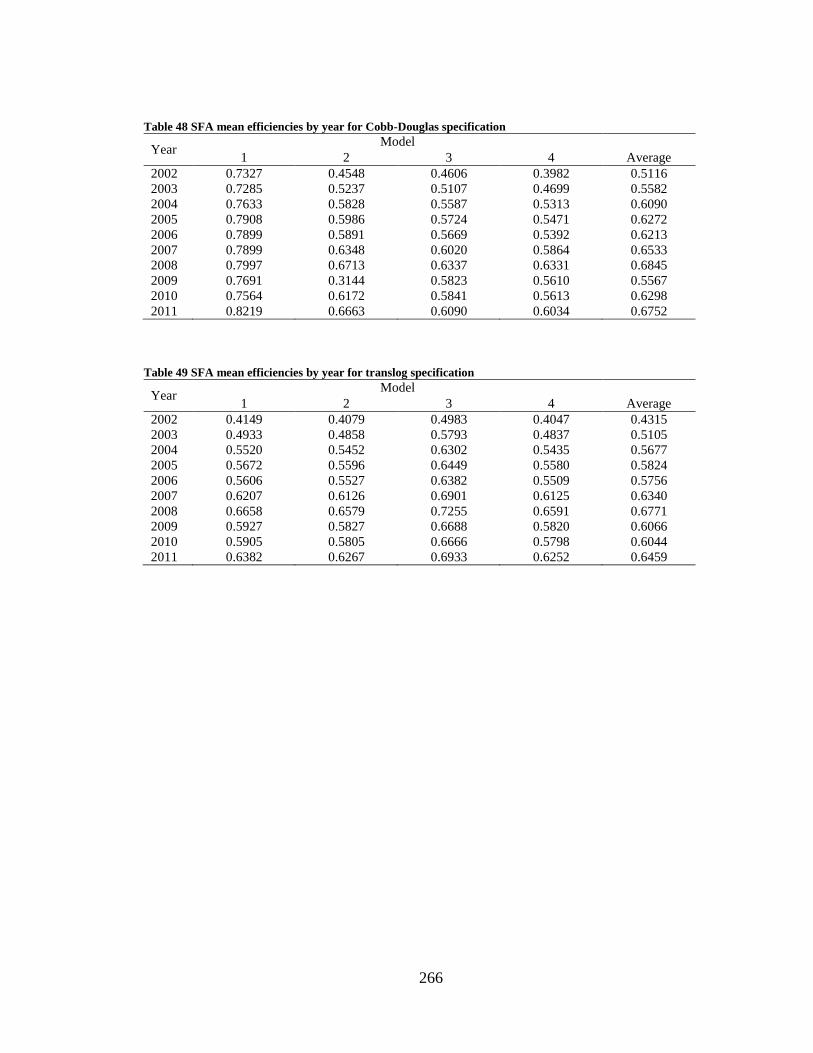
266

Table 48 SFA mean efficiencies by year for Cobb-Douglas specification

Year Model

1 2 3 4 Average

2002 0.7327 0.4548 0.4606 0.3982 0.5116

2003 0.7285 0.5237 0.5107 0.4699 0.5582

2004 0.7633 0.5828 0.5587 0.5313 0.6090

2005 0.7908 0.5986 0.5724 0.5471 0.6272

2006 0.7899 0.5891 0.5669 0.5392 0.6213

2007 0.7899 0.6348 0.6020 0.5864 0.6533

2008 0.7997 0.6713 0.6337 0.6331 0.6845

2009 0.7691 0.3144 0.5823 0.5610 0.5567

2010 0.7564 0.6172 0.5841 0.5613 0.6298

2011 0.8219 0.6663 0.6090 0.6034 0.6752

Table 49 SFA mean efficiencies by year for translog specification

Year Model

1 2 3 4 Average

2002 0.4149 0.4079 0.4983 0.4047 0.4315

2003 0.4933 0.4858 0.5793 0.4837 0.5105

2004 0.5520 0.5452 0.6302 0.5435 0.5677

2005 0.5672 0.5596 0.6449 0.5580 0.5824

2006 0.5606 0.5527 0.6382 0.5509 0.5756

2007 0.6207 0.6126 0.6901 0.6125 0.6340

2008 0.6658 0.6579 0.7255 0.6591 0.6771

2009 0.5927 0.5827 0.6688 0.5820 0.6066

2010 0.5905 0.5805 0.6666 0.5798 0.6044

2011 0.6382 0.6267 0.6933 0.6252 0.6459

267

APPENDIX IX – ANSP SFA ANALYSIS: FIGURES

Figure 19 SFA mean efficiencies by year for Cobb-Douglas specification

268

Figure 20 SFA mean efficiencies by year for translog specification

269

APPENDIX X – ANSP SFA ANALYSIS: REGRESSIONS

Table 50 SFA regression results for Cobb-Douglas specification

Model

1 2 3 4

Production

frontier

Intercept -3.0662***

(-14.670)

-3.5947*

(-1.833)

-1.6287***

(-5.374)

-2.6545***

(-10.739)

0.6777***

(17.991)

0.7543***

(3.909)

0.6300***

(15.279)

0.6675***

(16.288)

-0.0337**

(-2.938)

-0.0045

(-0.037)

-0.0325**

(-2.785)

-0.0157*

(-1.757)

0.1631***

(3.798)

0.1361

(1.545)

0.1096**

(2.224)

0.1567**

(3.127)

Technical

inefficiency

AGENCY 0.3945***

(4.215)

-0.2933

(-0.304)

-0.2104*

(-1.756)

-0.3701***

(-3.387)

AREA -0.0112***

(-7.409) -

-0.0013***

(-3.845) -

SECTORS -0.1650***

(-8.820)

-0.0196

(-1.442)

-0.0287***

(-3.522) -

ATCO 0.0090***

(8.426) - -

-0.006***

(-3.542)

ATCOkm -0.2466***

(-4.919)

0.2434**

(3.223) -

0.1054***

(3.702)

STAFF_ATCO 0.0379*

(1.845)

0.2224

(1.159) -

0.1551***

(5.708)

REV_COST -0.7533**

(-2.790)

-0.4156

(-0.541) -

-0.5824**

(-2.207)

Mean

inneficiency 77.5% 59.8% 57.0% 54.6%

Mean efficiency 22.5% 40.2% 43.0% 45.5%

0.0138 0.4429 0.2509 0.2537

0.0987 0.0297 0.0298 0.0059

λ2 0.1402 14.9039 8.4313 42.8957

Variance due to

inefficiency 12.3% 93.7% 89.4% 97.7%

Variance due to

random variation 87.7% 6.3% 10.6% 2.3%

Log likelihood -104.3407 -173.1192 -163.5451 -151.6983

Notes ***significant at 0.001; ** significant at 0.05; *significant at 0.1; z-values in parentheses.

Positive signs in the coefficients indicate that the variable is associated with larger levels of inefficiency.

270

Table 51 SFA regression results for translog specification

Model

1 2 3 4

Production

frontier

Intercept -8.9742***

(-5.836)

-8.8519***

(-5.882)

-6.0974***

(-6.175)

-8.5032***

(-5.627)

1.2224***

(3.690)

1.2175***

(3.872)

1.4273*

(1.936)

1.1153***

(3.620)

-0.2725**

(-2.422)

-0.2662**

(-2.589)

-0.1326

(-0.304)

-0.2402**

(-2.265)

0.9661*

(1.847)

0.9465**

(2.012)

0.0679

(0.112)

0.9588**

(2.049)

-0.2474**

(-3.162)

-0.2337**

(-2.837)

-0.3630

(-1.601)

-0.2402***

(-3.619)

0.0025

(0.080)

-0.0034

(-0.100)

-0.0555

(-1.224)

-0.0081

(-0.261)

0.1948*

(2.395)

0.1875**

(2.216)

0.3497

(1.306)

0.2073**

(2.920)

-0.0024

(-0.175)

-0.0056

(-0.394)

-0.0087

(-0.258)

-0.0063

(-0.484)

0.0223

(0.527)

0.0303

(0.649)

0.0742

(0.858)

0.0330

(0.798)

-0.2851**

(-2.669)

-0.2839**

(-2.616)

-0.4104

(-1.537)

-0.3064**

(-3.140)

Technical

inefficiency

AGENCY -0.4476**

(-3.136)

-0.4446***

(-3.441)

-0.5875

(-0.738)

-0.4409**

(-3.264)

AREA -0.0005

(-1.381) -

-0.0006

(-0.637) -

SECTORS -0.0324**

(-2.933)

-0.0175***

(-4.440)

-0.0145

(-1.577) -

ATCO 0.0009**

(2.065) - -

-0.0006***

(-4.079)

ATCOkm 0.1071**

(2.366)

0.1417***

(4.319) -

0.1300***

(4.247)

STAFF_ATCO 0.1733***

(4.638)

0.1685***

(6.249) -

0.1885***

(6.154)

REV_COST -0.0003

(-0.002)

-0.0342

(-0.266) -

-0.1278

(-0.778)

Mean

inneficiency 57.2% 56.4% 64.6% 56.3%

Mean efficiency 42.8% 43.6% 35.4% 43.8%

0.2649 0.2634 0.6099 0.2839

0.0049 0.0036 0.0230 0.0029

λ2

54.5020 73.6267 26.5634 97.1366

Variance due to

inefficiency 98.2% 98.7% 96.4% 99.0%

Variance due to

random variation 1.8% 1.3% 3.6% 1.0%

Log likelihood -104.3407 -173.1192 -163.5451 -151.6983

Notes ***significant at 0.001; ** significant at 0.05; *significant at 0.1; z-values in parentheses.

271

Positive signs in the coefficients indicate that the variable is associated with larger levels of inefficiency.

272

REFERENCES

Aigner, D., Lovell, C. A. K., & Schmidt, P. (1977). Formulation and Estimation of

Stochastic Frontier Production Function Models. Journal of econometrics, 6(1),

21–37.

Airways New Zealand. (2013). Annual Report 2012-13. Wellington, New Zealand:

Airways New Zealand.

Angrist, J. D., & Krueger, A. B. (1999). Empirical Strategies in Labor Economics. In O.

Ashenfelter & D. Card (Eds.), Handbook of Labor Economics (Vol. 3A, pp.

1277–1366). Amsterdam: Elsevier.

Assaf, A. (2010). The Cost Efficiency of Australian Airports Post Privatisation: A

Bayesian Methodology. Tourism Management, 31(2), 267–273.

Australian Competition and Consumer Commission. (2011). Airservices Australia Price

Notification - Final Decision. Canberra, Australia: Australian Competition and

Consumer Commission.

Averch, H., & Johnson, L. L. (1962). Behavior of the Firm Under Regulatory Constraint.

The American Economic Review, 52, 1052–1069.

Banker, R. D., Charnes, A., & Cooper, W. W. (1984). Some Models for Estimating

Technical and Scale Inefficiencies in Data Envelopment Analysis. Management

science, 30(9), 1078–1092.

Bertrand, M., Duflo, E., & Mullainathan, S. (2004). How Much Should We Trust

Differences-in-Differences Estimates? The Quarterly Journal of Economics,

119(1), 249–275.

Black, F. (1982). The Trouble With Econometric Models. Financial Analysts Journal,

38(2), 29–37.

Boardman, A. E., & Vining, A. R. (1989). Ownership and Performance in Competitive

Environments: A Comparison of the Performance of Private, Mixed, and State-

Owned Enterprises. Journal of Law and Economics, 32, 1.

273

Bogetoft, P., & Otto, L. (2011). Benchmarking with DEA, SFA, and R. New York, N.Y.:

Springer.

Borts, G. H. (1981). Report of the Managing Editor: American Economic Review.

American Economic Review, Papers and Proceedings, 71(2), 452– 464.

Bös, D. (1991). Privatization : a Theoretical Treatment. Oxford: Clarendon.

Button, K. (2004). Wings Across Europe : Towards an Efficient European Air Transport

System. Aldershot, Hampshire, England; Burlington, VT: Ashgate.

Button, K. (2008). Air Transportation Infrastructure in Developing Countries:

Privatization and Deregulation. In C. Winston & G. de Rus (Eds.), Aviation

Infrastructure Performance a Study in Comparative Political Economy.

Washington, D.C.: Brookings Institution Press.

Button, K. (2010). Transport Economics (3rd ed.). Northampton, MA: Edward Elgar

Publishing.

Button, K. (2013). A Book, the Application and the Outcomes; How Right was Alfred

Kahn in The Economics of Regulation about the Impacts of the Deregulation of

the US Domestic Airline Market? Working Paper.

Button, K. J., & Neiva, R. (2013). Economic Efficiency across National Air Navigation

Systems. Presented at the American Economics Association, 125th Annual

Meeting, San Diego, CA.

Button, K., & Johnson, K. (1998). Incremental Versus Trend-Break Change in Airline

Regulation. Transportation Journal, 37(3), 25–34.

Button, K., & McDougall, G. (2006). Institutional and Structure Changes in Air

Navigation Service-Providing Organizations. Journal of Air Transport

Management, 12(5), 236–252.

Camp, R. C. (1993). A Bible for Benchmarking, by Xerox. Financial Executive, 9(4),

23–27.

CANSO. (2010). Global Air Navigation Services Performance Report 2010. Amsterdam:

Civil Air Navigation Services Organisation.

CANSO. (2011). Global Air Navigation Services Performance Report 2011. Amsterdam:

Civil Air Navigation Services Organisation.

CANSO. (2012). Global Air Navigation Services Performance Report 2012. Amsterdam:

Civil Air Navigation Services Organisation.

274

Castelli, L., Labbé, M., & Violin, A. (2012). A Network Pricing Formulation for the

Revenue Maximization of European Air Navigation Service Providers.

Transportation Research Part C: Emerging Technologies. Retrieved from

http://www.sciencedirect.com/science/article/pii/S0968090X12000630

Caves, D. W., Christensen, L. R., & Diewert, W. E. (1982a). Multilateral Comparisons of

Output, Input, and Productivity Using Superlative Index Numbers. The economic

journal, 92(365), 73–86.

Caves, D. W., Christensen, L. R., & Diewert, W. E. (1982b). The Economic Theory of

Index Numbers and the Measurement of Input, Output, and Productivity.

Econometrica: Journal of the Econometric Society, 1393–1414.

Caves, R. E. (1962). Air Transport and Its Regulators: An Industry Study. Cambridge,

MA: Harvard University Press.

Charles, R. A., & Newman, H. K. (1995). Public Policy and Technology Management:

Changing the Role of Government in the Operation of Air Traffic Control.

Transportation Journal, 35(1), 39–48.

Charnes, A., Cooper, W. W., & Rhodes, E. (1978). Measuring the Efficiency of Decision

Making Units. European Journal of Operational Research, 2(6), 429–444.

Chermack, T. J., & Kasshanna, B. K. (2007). The Use and Misuse of SWOT Analysis

and Implications for HRD Professionals. Human Resource Development

International, 10(4), 383–399.

Civil Aviation Authority. (2011a). Air Traffic Services Licence for NATS (En Route) plc.

London, UK: Civil Aviation Authority.

Civil Aviation Authority. (2011b). UK Performance Plan for Air Navigation Services -

Reference Period One, 01 January 2012 to 31 December 2014. London, UK:

Civil Aviation Authority.

Coase, R. H. (1974). The Lighthouse in Economics. Journal of Law and Economics, 17,

357–376.

Coelli, T., Prasada Rao, D. S., & Battese, G. E. (1998). An Introduction to Efficiency and

Productivity Analysis. Boston: Kluwer Academic Publishers.

Competition Economists Group. (2011). Econometric Cost-Efficiency Benchmarking of

Air Navigation Service Providers. Brussels: EUROCONTROL.

Cook, A. (Ed.). (2007). European Air Traffic Management: Principles, Practice and

Research. Aldershot: Ashgate.

275

Cooper, W. W., Seiford, L. M., & Tone, K. (2007). Data Envelopment Analysis: a

Comprehensive Text with Models, Applications, References and DEA-Solver

Software. New York: Springer. Retrieved from

http://public.eblib.com/EBLPublic/PublicView.do?ptiID=323342

Coppin, C. A., & High, J. C. (1999). The Politics of Purity: Harvey Washington Wiley

and the Origins of Federal Food Policy. University of Michigan Press.

Cruz, C. O., & Marques, R. C. (2011). Contribution to the Study of PPP Arrangements in

Airport Development, Management and Operation. Transport Policy, 18(2), 392–

400.

Czerny, A. I. (2006). Price-Cap Regulation of Airports: Single-Till Versus Dual-Till.

Journal of Regulatory Economics, 30(1), 85–97.

Dattakumar, R., & Jagadeesh, R. (2003). A Review of Literature on Benchmarking.

Benchmarking: An International Journal, 10(3), 176–209.

Davies, A. J., & Kochhar, A. K. (2002). Manufacturing Best Practice and Performance

Studies: a Critique. International Journal of Operations & Production

Management, 22(3), 289–305.

De Neufville, R. (1999). Airport Privatization: Issues for the United States.

Transportation Research Record: Journal of the Transportation Research Board,

1662, 24–31.

De Neufville, R., & Odoni, A. R. (2002). Airport Systems : planning, design, and

management. London: McGraw-Hill.

Dempsey, P. S., Janda, R., Nyampong, Y., Saba, J., & Wilson, J. (2005). The McGill

Report on Governance of Commercialized Air Navigation Services. Montreal:

McGill University Center for Research on Air & Space Law.

Demsetz, H. (1968). Why regulate utilities? Journal of Law and Economics, 11(1), 55–

65.

Domney, M., Wilson, H. I. M., & Chen, E. (2005). Natural Monopoly Privatisation

Under Different Regulatory Regimes: A Comparison of New Zealand and

Australian Airports. International Journal of Public Sector Management, 18(3),

274–292.

EUROCONTROL. (2013). U.S. - Europe Continental Comparison of ANS Cost-

Efficiency Trends (2002-2011). Brussels: EUROCONTROL.

276

EUROCONTROL Performance Review Commission. (2001). Cost Effectiveness and

Productivity KPIs. Working Paper.

EUROCONTROL Performance Review Commission. (2005a). A Comparison of

Performance in Selected US and European En-route Centres. Brussels:

EUROCONTROL.

EUROCONTROL Performance Review Commission. (2005b). Total Factor Productivity

of European Air Navigation Services Providers: Basic Concepts and Empirical

Application. Brussels: EUROCONTROL.

EUROCONTROL Performance Review Commission. (2007). Evaluation of

Civil/Military Airspace Utilisation. Brussels: EUROCONTROL.

EUROCONTROL Performance Review Commission. (2008). Evaluation of Functional

Airspace Block (FAB) Initiatives and their Contribution to Performance

Improvement. Brussels: EUROCONTROL.

EUROCONTROL Performance Review Commission. (2012). ATM Cost-Effectiveness

(ACE) 2010 Benchmarking Report with 2011-2015 outlook. Brussels:

EUROCONTROL.

EUROCONTROL Performance Review Commission. (2013a). ATM Cost-Effectiveness

(ACE) 2011 Benchmarking Report with 2012-2016 outlook. Brussels:

EUROCONTROL.

EUROCONTROL Performance Review Commission. (2013b). Performance Review

Report - An Assessment of Air Traffic Management in Europe during the

Calendar Year 2012. Brussels: EUROCONTROL.

EUROCONTROL Performance Review Commission, & Federal Aviation

Administration. (2009). U.S./Europe Comparison of ATM-related Operational

Performance. Brussels/Washington DC: EUROCONTROL/FAA.

EUROCONTROL Performance Review Commission, & Federal Aviation

Administration. (2012). 2010 US/Europe Comparison of ATM-Related

Operational Performance. Brussels/Washington DC: EUROCONTROL/FAA.

EUROCONTROL Performance Review Commission, & Federal Aviation

Administration. (2013). 2012 - Comparison of Air Traffic Management-Related

Operational Performance: U.S./Europe. Brussels/Washington DC:

EUROCONTROL/FAA.

European Commission. (2012a). Functional Airspace Blocks (FABs). Retrieved from

http://ec.europa.eu/transport/modes/air/single_european_sky/fab/

277

European Commission. (2012b). Single European Sky. Retrieved from

http://ec.europa.eu/transport/modes/air/single_european_sky/

European Economic Community. (1957). Treaty of Rome. Rome. Retrieved from

http://ec.europa.eu/economy_finance/emu_history/documents/treaties/rometreaty2

.pdf

Farrell, M. J. (1957). The Measurement of Productive Efficiency. Journal of the Royal

Statistical Society. Series A (General), 120(3), 253–290.

Federal Aviation Administration. (2008). Instrument Flying Handbook. Washington DC.

Federal Aviation Administration. (2013). NextGen. Retrieved from

http://www.faa.gov/nextgen/

Forsyth, P. (2001). Airport Price Regulation: Rationales, Issues and Directions for

Reform. Monash University. Retrieved from

http://www.pc.gov.au/__data/assets/pdf_file/0004/19840/sub005.pdf

Fried, H. O., Lovell, C. A. K., & Schmidt, S. S. (2008a). Efficiency and Productivity. In

H. O. Fried, C. A. K. Lovell, & S. S. Schmidt (Eds.), The Measurement of

Productive Efficiency and Productivity Change. New York: Oxford University

Press.

Fried, H. O., Lovell, C. A. K., & Schmidt, S. S. (Eds.). (2008b). The Measurement of

Productive Efficiency and Productivity Change. New York: Oxford University

Press.

Glaeser, E. L., & Shleifer, A. (2003). The Rise of the Regulatory State. Journal of

Economic Literature, 41(2), 401–425.

Golaszewski, R. (2002). Reforming Air Traffic Control: An Assessment from the

American Perspective. Journal of Air Transport Management, 8(1), 3–11.

Goodliffe, M. (2002). The New UK Model for Air Traffic Services - A Public Private

Partnership Under Economic Regulation. Journal of Air Transport Management,

8(1), 13–18.

Heckman, J. J., & Vytlacil, E. J. (2007). Econometric Evaluation ofSocial Programs, Part

I: Causal Models, Structural Models and Econometric Policy Evaluation.

Handbook of Econometrics, 6, 4779–4874.

Helios Economics and Policy Services. (2006a). Cost Benchmarking of NATS Relative to

Selected Air Navigation Service Providers - Phase 2 Report. Farnborough, UK:

UK Civil Aviation Authority - Economic Regulation Group.

278

Helios Economics and Policy Services. (2006b). The Impact of Fragmentation in

European ATM/CNS. Farnborough, UK: EUROCONTROL.

Helms, M. M., & Nixon, J. (2010). Exploring SWOT Analysis – Where Are We Now?: A

Review of Academic Research from the Last Decade. Journal of Strategy and

Management, 3(3), 215–251.

Henry, C., Matheu, M., & Jeunemaître, A. (Eds.). (2001). Regulation of Network

Utilities: The European Experience. Oxford University Press.

High, J. (Ed.). (1991). Regulation: Economic Theory and History. Ann Arbor: University

of Michigan Press.

International Civil Aviation Organization. (2006). Convention on International Civil

Aviation - Doc 7300/9. Montréal, Canada: International Civil Aviation

Organization.

Irish Aviation Authority, & NATS. (2012). UK-Ireland FAB Annual Report 2011.

Dublin/London: Irish Aviation Authority/NATS.

Jasiński, P., & Yarrow, G. (1996). Privatization: an Overview of the Issues. In G. Yarrow

& P. Jasiński (Eds.), Privatization: Critical Perspectives on the World Economy,

Volume I. London: Routledge.

Kahn, A. E. (1970). The Economics of Regulation: Principles and Institutions. Volumes I

& II. New York: John Wiley & Sons.

Kahn, A. E. (2004). Lessons From Deregulation : Telecommunications and Airlines After

the Crunch. Washington, D.C.: AEI-Brookings Joint Center for Regulatory

Studies : [Distributed by] Brookings Institution Press.

Koch, A. J. (2000). SWOT Does Not Need to be Recalled: It Needs to be Enhanced.

Business Quest. Retrieved from http://en.scientificcommons.org/48903374

Kolko, G. (1963). The Triumph of Conservatism: A Reinterpretation of American

History, 1900-1916. New York: Free Press of Glencoe.

Kraus, T. L. (2011). Celebrating 75 Years of Federal Air Traffic Control. Washington,

D.C.: Federal Aviation Administration.

Laffont, J.-J., & Tirole, J. (1993). A Theory of Incentives in Procurement and Regulation.

Cambridge, Mass.: MIT Press.

Laffont, J.-J., & Tirole, J. (2000). Competition in Telecommunications. Cambridge,

Mass.: MIT Press.

279

Leibenstein, H. (1966). Allocative Efficiency vs.“ X-efficiency.” The American

Economic Review, 56(3), 392–415.

Levine, M. E. (1964). Is Regulation Necessary? California Air Transportation and

National Regulatory Policy. Yale Law Journal, 74, 1416.

Majumdar, A. (1995). Commercializing and Restructuring Air Traffic Control: A Review

of the Experience and Issues Involved. Journal of Air Transport Management,

2(2), 111–122.

mbs ottawa inc. (2006). Air Traffic Control Commercialization Policy: Has It Been

Effective? Ottawa: mbs ottawa inc.

McCraw, T. K. (1984). Prophets of Regulation. Belknap Press.

McDougall, G., & Roberts, A. (2008). Commercializing Air Traffic Control: Have the

Reforms Worked? Canadian Public Administration / Administration Publique du

Canada, 51(1), 45–69.

McInally, J. (2010). EUROCONTROL History Book. Brussels: EUROCONTROL.

Meeusen, W., & van den Broeck, J. (1977). Efficiency Estimation From Cobb-Douglas

Production Functions With Composed Error. International Economic Review,

435–444.

Merkert, R., Odeck, J., Brathen, S., & Pagliari, R. (2012). A Review of Different

Benchmarking Methods in the Context of Regional Airports. Transport Reviews,

32(3), 379–395.

Moran, P. A. P. (1950). Notes on Continuous Stochastic Phenomena. Biometrika,

37(1/2), 17–23.

Morrison, S. A., & Winston, C. (2008). The Effect of FAA Expenditures on Air Travel

Delays. Journal of Urban Economics, 63(2), 669–678.

National Civil Aviation Review Commission. (1997). Avoiding Aviation Gridlock and

Reducing the Accident Rate - A Consensus for Change. Washington DC.

NAV Canada. (2013). 2012 Annual Report. Ottawa, Canada: NAV Canada.

Nett, L. (1994). Why Private Firms Are More Innovative Than Public Firms. European

Journal of Political Economy, 10(4), 639–653.

Nolan, M. S. (1998). Fundamentals of Air Traffic Control. Pacific Groove: Brooks/Cole :

Wadsworth.

280

Odland, J. (1988). Spatial Autocorrelation. Newbury Park, CA: SAGE Publications.

Office of Inspector General. (1998). Advance Automation System - Federal Aviation

Administration. Washington, D.C.: Department of Transportation.

Oster, C. V., & Strong, J. S. (2006). Reforming the Federal Aviation Administration:

Lessons from Canada and the United Kingdom. Washington, D.C.: The IBM

Center for The Business of Government.

Oster, C. V., & Strong, J. S. (2007). Managing the Skies: Public Policy, Organization

and Financing of Air Traffic Management. Aldershot, England; Burlington, VT:

Ashgate.

Oum, T. H., Adler, N., & Yu, C. (2006). Privatization, Corporatization, Ownership Forms

and their Effects on the Performance of the World’s Major Airports. Journal of

Air Transport Management, 12(3), 109–121.

Oum, T. H., Yan, J., & Yu, C. (2008). Ownership Forms Matter for Airport Efficiency: A

Stochastic Frontier Investigation of Worldwide Airports. Journal of Urban

Economics, 64(2), 422–435.

Oum, T. H., & Yu, C. (1995). A Productivity Comparison of the World’s Major Airlines.

Journal of Air Transport Management, 2(3), 181–195.

Oum, T. H., Zhang, A., & Zhang, Y. (2004). Alternative Forms of Economic Regulation

and their Efficiency Implications for Airports. Journal of Transport Economics

and Policy, 38(2), 217–246.

Peltzman, S. (1976). Toward a More General Theory of Regulation. National Bureau of

Economic Research Cambridge, Mass., USA.

Peltzman, S., & Winston, C. (Eds.). (2000). Deregulation of Network Industries: What’s

Next? Washington, D.C.: AEI-Brookings Joint Center for Regulatory Studies.

Posner, R. A. (1971). Taxation by Regulation. The Bell Journal of Economics and

Management Science, 2(Spring 1971), 22–50.

Post, T. (2001). Performance Evaluation in Stochastic Environments Using Mean-

Variance Data Envelopment Analysis. Operations Research, 49(2), 281–292.

Reinhold, A., Niemeier, H.-M., Kamp, V., & Müller, J. (2010). An Evaluation of

Yardstick Regulation for European Airports. Journal of Air Transport

Management, 16(2), 74–80.

Robyn, D. (2007). Reforming the Air Traffic Control System to Promote Efficiency and

Reduce Delays. The Brattle Group, Inc and GRA Inorporated.

281

Rose, N. L. (2012). After Airline Deregulation and Alfred E. Kahn. American Economic

Review, 102(3), 376–380.

Savas, E. (2000). Privatization and Public-Private Partnerships. New York: Chatham

House.

Schaar, C. (2010). A Method for Stakeholder-Based Comparative Benchmarking of

Airports (Ph.D. Dissertation). George Mason University, Fairfax, VA.

Schaar, C., & Sherry, L. (2008). Comparison of Data Envelopment Analysis Methods

Used in Airport Benchmarking. Presented at the 3rd International Conference on

Research in Air Transportation – ICRAT 2008, Fairfax, VA.

Simar, L., & Wilson, P. W. (1998). Sensitivity Analysis of Efficiency Scores: How to

Bootstrap in Nonparametric Frontier Models. Management science, 44(1), 49–61.

Simar, L., & Wilson, P. W. (2007). Estimation and Inference in Two-Stage, Semi-

Parametric Models of Production Processes. Journal of econometrics, 136(1), 31–

64.

Simon, H. A. (1956). Rational Choice and the Structure of the Environment.

Psychological review, 63(2), 129–138.

Steuer, M. (2010). The Partially Private UK System for Air Traffic Control. Journal of

air transport management, 16(1), 26–35.

Stigler, G. J. (1971). The Theory of Economic Regulation. The Bell journal of economics

and management science, 3–21.

Syverson, C. (2011). What Determines Productivity? Journal of Economic Literature,

49(2), 326–365.

Thornton, R. L. (1977). Deregulation: the CAB and its Critics. Journal of Air Law and

Commerce, 43, 641.

Tobler, W. R. (1970). A Computer Movie Simulating Urban Growth in the Detroit

Region. Economic geography, 46, 234–240.

Train, K. (1991). Optimal Regulation: the Economic Theory of Natural Monopoly.

Cambridge, MA: MIT Press.

Tzu, S. (2005). The Art of War. (L. Giles, Trans., J. H. Ford & Shawn Conners, Eds.). El

Paso, TX: El Paso Norte Press.

282

United States Government Accountability Office. (2005). Air Traffic Control:

Characteristics and Performance of Selected International Air Navigation Service

Providers and Lessons Learned from their Commercialization. Washington DC.

United States Government Accountability Office. (2010a). Next Generation Air

Transportation System - Challenges with Partner Agency and FAA Coordination

Continue, and Efforts to Integrate Near-, Mid-, and Long-term Activities Are

Ongoing. Washington DC.

United States Government Accountability Office. (2010b). Next Generation Air

Transportation System - FAA’s Metrics Can Be Used to Report on Status of

Individual Programs, but Not of Overall NextGen Implementation or Outcomes.

Washington DC.

United States Government Accountability Office. (2011a). Next Generation Air

Transportation System - Collaborative Efforts with European Union Generally

Mirror Effective Practices, but Near-Term Challenges Could Delay

Implementation. Washington DC.

United States Government Accountability Office. (2011b). Next Generation Air

Transportation System - FAA Has Made Some Progress in Implementation, but

Delays Threaten to Impact Costs and Benefits. Washington DC.

United States Government Accountability Office. (2012a). Air Traffic Control

Modernization - Management Challenges Associated with Program Costs and

Schedules Could Hinder NextGen Implementation. Washington DC.

United States Government Accountability Office. (2012b). Next Generation Air

Transportation System - FAA Faces Implementation Challenges. Washington

DC.

United States Government Accountability Office. (2013). Next Generation Air

Transportation System - FAA Has Made Some Progress in Midterm

Implementation, but Ongoing Challenges Limit Expected Benefits. Washington

DC.

Vietor, R. (1991). The Hubris of Regulated Competition: Airlines, 1925-88. In J. High

(Ed.), Regulation: Economic Theory and History. Ann Arbor: University of

Michigan Press.

Vogel, H.-A. (2004, April). Airport Privatisation and Perfomance (Ph.D. Dissertation).

University of Westminster, London, UK.

Waldman, D. E., & Jensen, E. J. (2007). Industrial Organization: Theory and Practice.

Boston: Pearson Addison Wesley.

283

Ward, M. D., & Gleditsch, K. S. (2008). Spatial Regression Models. Thousand Oaks,

CA: SAGE Publications.

Wei, W., & Hansen, M. (2005). Impact of Aircraft Size and Seat Availability on Airlines’

Demand and Market Share in Duopoly Markets. Transportation Research Part E:

Logistics and Transportation Review, 41(4), 315–327.

Williamson, O. E. (1976). Franchise Bidding for Natural Monopolies - In General and

With Respect to CATV. The Bell Journal of Economics, 73–104.

Winston, C. (2012). Government Policy for a Partially Deregulated Industry: Deregulate

it Fully. American Economic Review, 102(3), 391–395.

Yarrow, G., & Jasiński, P. (Eds.). (1996). Privatization: Critical Perspectives on the

World Economy, Volumes I, II, III, IV. London: Routledge.

284

BIOGRAPHY

Rui Neiva has a background in Civil Engineering. He earned his bachelor’s (2007) and

master’s (2009) degree from the Faculty of Engineering of the University of Porto,

Portugal.