Economic assessment of storage in residential

microgrids

Kevin Milis

Promotors:

Prof. dr. Herbert Peremans

Prof. dr. Steven Van Passel

ii

Preface

�Non nobis solum nati sumus� -

We are not born for ourselves

alone

Cicero, De O�ciis - On Duties

I:22

It is said that it is the mark of advanced civilisations that some of theirmembers can devote themselves to pursuits other than those directly relatedto the production of food and other goods. I am one of those lucky few, inthat I have been allowed to spend six years researching the topic of storage inmicrogrids, which has culminated in the dissertation you are now reading. APhD dissertation in itself has of course a procedural value, in that it shouldshow that the author is ready to e�ectuate his or her own independent re-search. However, I think it is important to echo the sentiment contained inthe quote above, so it is important to broaden the scope of re�ection, andnot only think about what this dissertation signi�es for its author: societyhas funded the research this dissertation is based upon, so it is only naturalto consider the bene�ts of this work to society.

The more cynical amongst us might be quick to quip that the main bene�tof funding PhD scholarships for society is that it keeps people like the authorsafely away from the more directly productive elements of society, and whileit is true that no academic spin-o�s or patent applications resulted from thisresearch, I am nevertheless inclined to disagree, and defend the position thatthere most certainly is a bene�t to society: not only does each phd signifythat one more member of society is now trained in knowledge creation, andtherefore ready to help broaden and deepen the breadth of human under-standing, but also in the speci�c case of this phd, the interested reader will�nd that policy recommendations are included within, aimed at aiding cli-mate change mitigation through increasing the uptake of storage, therebyallowing for a greater penetration of renewable energy sources. While some

iii

might claim that it is nebulous how this relates to increasing shareholdervalue, it is crystal clear how this is aimed at creating stakeholder value.

Similarly to how I did not write this dissertation just for myself, I was alsonot alone during the creation of it: the many colleagues of the departmentof engineering management created a productive and enjoyable atmosphereto work in, fostering positive professional relationships which has helped tre-mendously in making light work of the work that needed to be done. Thispositive atmosphere is in place largely thanks to the e�orts of the facultyof the department, who strive to keep the working environment open andcollaborative, regardless of who is in the current batch of phd candidates.To all colleagues, past and present, a heartfelt thank you for the professionalcameraderie.

There are some people who I would like to thank by name, for the singularimpact they have had on me and my work: �rst and foremost, my promo-tors, Herbert, for your constant support, your razor sharp eye where typosor spurious arguments are concerned and your non-economical background,which ensured that �that's how everyone else is doing it� was never reasonenough; and Steven, for your tips and tricks surrounding academic trade-craft, opening my eyes to the policy related side of research and for access toyour network, thank you both. Johan, thank you for your readiness and will-ingness to help with a myriad of professional quandaries, related to teaching,research, or administration, for your methodological pointers and for tying toshield us graduate students as best as possible from academic manoeuvringby serving as department head. Trijntje, thank you for listening wheneversomething I got worked up, and thank you for your insightful remarks, whichalways prompt me to introspection and help me to grow professionally. Iwould of course also like to thank the members of my jury, for your com-ments and remarks, which have helped in perfecting this dissertation.

Of course, work and the o�ce are but parts of one's life, the other part beingfriends and family. Without my friends, it would have been hard to remaingrounded, as they provided an invaluable look on life outside academia, eventhough some colleague became friends while other friends became colleagues.My �nal, and most heartfelt, thanks is reserved for my parents: not onlyfor shaping me into the man I am today, but also for their continuous andunfaltering support as well as their strong focus on ensuring I got a goodeducation. Thanks also for supporting my choice when I decided I wantedto go into academia, even if neither of you could at �rst really envisage whatthat would mean. Furthermore, you also always ensured that home truly

iv

was and is a safe port in any storm, meaning that no matter what happens,I can always rest and recover there, always enabling me to go on.

Finally, in closing, I hope that through reading this work, you, the readercan enjoy at least part of the joy and intellectual enrichment I experiencedwhile working on it.

Kevin MilisAntwerp

August 2018

v

vi

Dutch synopsis

Dit werk heeft als onderwerp de bepaling van de economische waarde vanopslag in residentiële microgrids. Een microgrid is een onderdeel van eennutsvoorzieningsnetwerk dat in staat is om ook los van dit netwerk te func-tioneren, wat wil zeggen dat een microgrid zowel opwekking als verbruikvan elektrische energie bevat, en in staat moet zijn om deze vraag en ditaanbod op elkaar af te stemmen. Microgrids dienen gezien te worden inhet kader van het streven naar een duurzamere energievoorziening: één vande grootste troeven van een microgrid is immers dat het grotere penetra-tie van hernieuwbare energiebronnen faciliteert, daar een microgird werktvolgens het paradigma dat de vraag de opwekking volgt. Een belangrijkecomponent van een microgrid ter ondersteuning van dit paradigma is de op-slagcomponent: deze component laat immers toe om, binnen de grenzen vande beschikbare capaciteit, vraag en opwekking van elkaar los te koppelen.In tegenstelling echter tot kleinschalige, lokale opwekking -denk bijvoorbeeldaan zonnepanelen- komt lokale elektrische opslag niet echt van de grond.

De hierboven beschreven observatie geeft aanleiding tot de volgende onder-zoeksvraag: Wat is de huidige economische waarde van opslag voor de eige-naar van een residentieel microgrid, en in het geval dat deze waarde negatiefzou zijn, wat zijn dan beleidsinterventies die hier verandering in kunnen bren-gen? Deze centrale onderzoeksvraag wordt opgesplitst in drie meer speci�ekeonderzoeksvragen:

• Wat is de huidige economische waarde van opslag voor een residentiëlemicrogrid-eigenaar?

• Wat is een goede manier om microgrids te modeleren en beleidsinter-venties te onderzoeken?

• Welke beleidsinterventies moedigen de instalatie van opslag in een resi-dentieel microgrid aan?

vii

Hoofdstuk twee beantwoordt de eerste speci�eke onderzoeksvraag: litera-tuuronderzoek toont immers duidelijk aan dat opslag geen deel uitmaaktvan de economisch optimale systeemcon�guratie, tenzij er sprake is vansteunmaatregelen die er speci�ek op gericht zijn om opslag aan te moedi-gen. Voorts is het echter wel opvallend dat er slechts een betrekkelijk nauwgamma aan verschillende beleidsinterventies wordt onderzocht in de litera-tuur: de nadruk ligt bijna uitsluitend op feed-in tari�s en belastingsaftrekkenvan investeringen.

Als antwoord op de tweede onderzoeksvraag wordt in hoofdstuk drie en viereen simulatiemodel voor een microgrid opgesteld, en wordt een heuristischemethode voorgesteld om het kostenminimalisatieprobleem op te lossen. Dezeontwikkelde methodologie laat dan toe om verschillende beleidsinterventieste onderzoeken, wat meteen ook toelaat om de derde vraag te beantwoor-den. Uit dit onderzoek komt naar voor dat een capaciteitstarief, waarbij deelektriciteitsfactuur van de gebruiker niet enkel afhangt van de totale hoeveel-heid gebruikte energie over de facturatieperiode, maar ook van de individuelevraagpieken tijdens de facturatiepieken een zeer beloftevolle piste is. Het uit-gevoerde onderzoek toont immers niet enkel aan dat zo'n capaciteitstarief deinstallatie van batterijopslag zou bevorderen bij huishoudens met zonnepa-nelen, maar bovendien ook zou toelaten om investeringen in het uitbreidenvan de capaciteit van het distributienet uit te stellen.

viii

Contents

Preface iii

Dutch synopsis vii

Contents ix

List of Figures xiii

List of Tables xv

1 Introduction 1

1.1 Towards microgrids . . . . . . . . . . . . . . . . . . . . . . . . 11.2 Research question and contribution . . . . . . . . . . . . . . . 41.3 Methods . . . . . . . . . . . . . . . . . . . . . . . . . . . . . . 61.4 Structure . . . . . . . . . . . . . . . . . . . . . . . . . . . . . 6

2 The impact of policy on microgrid economics: a review 11

2.1 Introduction . . . . . . . . . . . . . . . . . . . . . . . . . . . . 122.2 Methodology . . . . . . . . . . . . . . . . . . . . . . . . . . . 14

2.2.1 Objective functions and decision variables . . . . . . . 162.2.2 Simulation set-up . . . . . . . . . . . . . . . . . . . . . 17

2.3 Technology and Policy . . . . . . . . . . . . . . . . . . . . . . 192.3.1 Technologies . . . . . . . . . . . . . . . . . . . . . . . . 202.3.2 Policy measures . . . . . . . . . . . . . . . . . . . . . . 20

2.4 Reported results . . . . . . . . . . . . . . . . . . . . . . . . . . 222.4.1 Business as usual . . . . . . . . . . . . . . . . . . . . . 222.4.2 Carbon taxation . . . . . . . . . . . . . . . . . . . . . 232.4.3 Economic incentives . . . . . . . . . . . . . . . . . . . 242.4.4 Tari� systems . . . . . . . . . . . . . . . . . . . . . . . 252.4.5 Command and control policies . . . . . . . . . . . . . . 25

2.5 Discussion . . . . . . . . . . . . . . . . . . . . . . . . . . . . . 262.6 Conclusion . . . . . . . . . . . . . . . . . . . . . . . . . . . . . 29

ix

3 Economical optimization of microgrids: a non-causal model 35

3.1 Introduction . . . . . . . . . . . . . . . . . . . . . . . . . . . . 373.2 Model overview and components . . . . . . . . . . . . . . . . . 383.3 Cost minimisation . . . . . . . . . . . . . . . . . . . . . . . . . 413.4 Storage use strategies . . . . . . . . . . . . . . . . . . . . . . . 43

3.4.1 Strategy 1: Passive Storage Use . . . . . . . . . . . . . 453.4.2 Strategy 2: Price Arbitrage . . . . . . . . . . . . . . . 453.4.3 Strategy 3: Back-up Power . . . . . . . . . . . . . . . . 46

3.5 Simulation . . . . . . . . . . . . . . . . . . . . . . . . . . . . . 463.6 Results and limitations . . . . . . . . . . . . . . . . . . . . . . 503.7 Conclusion . . . . . . . . . . . . . . . . . . . . . . . . . . . . . 52

4 Win-win possibilities through capacity tari�s and battery

storage in microgrids 55

4.1 Introduction . . . . . . . . . . . . . . . . . . . . . . . . . . . . 564.2 Methods . . . . . . . . . . . . . . . . . . . . . . . . . . . . . . 57

4.2.1 Problem formulation . . . . . . . . . . . . . . . . . . . 584.2.2 Heuristic solution method . . . . . . . . . . . . . . . . 624.2.3 Simulation set-up . . . . . . . . . . . . . . . . . . . . . 67

4.3 Results and discussion . . . . . . . . . . . . . . . . . . . . . . 684.3.1 Results without dimensionality reduction . . . . . . . . 684.3.2 Dimensionality reduction . . . . . . . . . . . . . . . . . 724.3.3 Results with dimensionality reduction . . . . . . . . . . 76

4.4 Conclusion . . . . . . . . . . . . . . . . . . . . . . . . . . . . . 79

5 Steering the adoption of battery storage through electricity

tari� design 87

5.1 Introduction . . . . . . . . . . . . . . . . . . . . . . . . . . . . 875.2 Literature review . . . . . . . . . . . . . . . . . . . . . . . . . 895.3 Research goal & hypothesis . . . . . . . . . . . . . . . . . . . 905.4 Research Methodology . . . . . . . . . . . . . . . . . . . . . . 91

5.4.1 Reserach method . . . . . . . . . . . . . . . . . . . . . 925.4.2 Reseerach variables . . . . . . . . . . . . . . . . . . . . 945.4.3 Design of the simulation model . . . . . . . . . . . . . 96

5.5 Results and discussion . . . . . . . . . . . . . . . . . . . . . . 985.6 Conclusion . . . . . . . . . . . . . . . . . . . . . . . . . . . . . 108

6 Conclusion 123

6.1 Addressing the research question . . . . . . . . . . . . . . . . 1236.2 Key messages beyond the research question . . . . . . . . . . . 1256.3 Limitations . . . . . . . . . . . . . . . . . . . . . . . . . . . . 126

x

6.4 Future outlook . . . . . . . . . . . . . . . . . . . . . . . . . . 127

xi

xii

List of Figures

1.1 Dissertation strucuture . . . . . . . . . . . . . . . . . . . . . . 5

3.1 Model components and transaction boundary . . . . . . . . . 363.2 Pattern of electricity spot prices . . . . . . . . . . . . . . . . . 443.3 Strategy �owcharts . . . . . . . . . . . . . . . . . . . . . . . . 443.4 Simulation results: scenario 1 . . . . . . . . . . . . . . . . . . 483.5 Simulation results: scenario 2 . . . . . . . . . . . . . . . . . . 483.6 Simulation results: scenario 3 . . . . . . . . . . . . . . . . . . 493.7 Simulation results: varying grid reliability . . . . . . . . . . . 493.8 Charge and discharge thresholds for strategy 2 . . . . . . . . . 49

4.1 Model con�gurations . . . . . . . . . . . . . . . . . . . . . . . 574.2 Heuristic �owcharts . . . . . . . . . . . . . . . . . . . . . . . . 634.3 Overview of the di�erent bases . . . . . . . . . . . . . . . . . . 664.4 Block capacity tari� . . . . . . . . . . . . . . . . . . . . . . . 684.5 Normalised weights of the basis vectors . . . . . . . . . . . . . 75

5.1 Model con�gurations . . . . . . . . . . . . . . . . . . . . . . . 925.2 Second week of January for scenario A . . . . . . . . . . . . . 995.3 Second week of January for scenario B . . . . . . . . . . . . . 1005.4 Second week of January for scenario B . . . . . . . . . . . . . 1015.5 Storage state: 1.8 kWh . . . . . . . . . . . . . . . . . . . . . . 1035.6 Storage state: 1.8 kWh . . . . . . . . . . . . . . . . . . . . . . 1035.7 Projected costs per 24 hours in e for Scenario B . . . . . . . . 1055.8 Projected costs per 24 hours in e for Scenario C . . . . . . . . 106

xiii

xiv

List of Tables

2.1 Optimisation objectives and decision variables . . . . . . . . . 152.2 Simulation set-up . . . . . . . . . . . . . . . . . . . . . . . . . 172.3 Technology capital cost . . . . . . . . . . . . . . . . . . . . . . 182.4 Technology yearly maintenance and operational costs. . . . . . 182.5 Technology and policy matrix. . . . . . . . . . . . . . . . . . . 19

3.1 Simulation parameter settings . . . . . . . . . . . . . . . . . . 46

4.1 Results: block capacity pricing, no PV . . . . . . . . . . . . . 724.2 Results: block capacity pricing & PV . . . . . . . . . . . . . . 724.3 Results: �xed capacity pricing, no PV . . . . . . . . . . . . . 734.4 Results: �xed capacity pricing & PV . . . . . . . . . . . . . . 734.5 Results: no capacity pricing, no PV . . . . . . . . . . . . . . . 734.6 Results: no capacity pricing, with PV . . . . . . . . . . . . . . 744.7 Results: block capicity pricing, no PV revisited . . . . . . . . 774.8 Results: block capacity pricing & PV revisited . . . . . . . . . 784.9 Results: �xed capacity pricing, no PV revisited . . . . . . . . 784.10 Results:�xed capacity pricing & PV revisted . . . . . . . . . . 78

5.1 Pricing and tari� design scenarios . . . . . . . . . . . . . . . . 955.2 Capacity prices . . . . . . . . . . . . . . . . . . . . . . . . . . 965.3 Descriptive statsitics of the exogenous data sets . . . . . . . . 985.4 Simulation results . . . . . . . . . . . . . . . . . . . . . . . . . 104

xv

xvi

Chapter 1

Introduction

1.1 Towards microgrids

Electricity is omnipresent in today's society: without it, the industrial sectorand services sector would come to halt. Electricity use is also making inroadsinto the transportation sector: e-bikes and electrical cars are newer entries tothe electri�ed transportation options, alongside the electrical train and tram.Furthermore, electricity is also increasingly gaining further importance whenit comes to leisure activities: electricity powers our tv's, our computers andour smartphones.

While it is neigh impossible to overstate the importance of electricity intoday's society, generation of electricity using conventional means has comeunder increasing scrutiny over the years. With regards to fossil fuels, thereare concerns surrounding the depletion of the �nite supply of those fuels[1],and while this peak oil issue has been contentious [2], probable oil reserveskeep increasing. A more stringent issue facing electricity generation fromfossil fuels, is global climate change, which if unabated, is project to causedrastic changes in the landscape due to rising sea levels as well as seriouseconomic damages [4]. According to data released by the IPCC, the electri-city supply sector was responsible for 35% of all anthropogenic greenhousegas emissions in 2010 [5]. Similarly, electricity generation using nuclear �s-sion is not without drawbacks: there is the problem of the long term safestorage of the generated nuclear waste on the one hand, and the devast-ating consequences of a nuclear accident in terms of loss of life, economicdamages and environmental impacts as evidenced by the nuclear accidentsin Chernobyl and Fukushima on the other hand. Furthermore, there arealso the high costs associated with decommissioning a nuclear power plant

1

at the end of its life cycle [6]. A �nal member of the group of traditionalpower generation techniques is hydro-electrical power generation, and whileits use isn't as heavily contested as the other generation techniques, it hasthe problem of being limited in possible deployments due to the fact that itneeds rather speci�c circumstances, namely the availability of a water reser-voir and a su�cient di�erence in height, for it to be viable. Nevertheless, it isnot an insigni�cant power source, as Eurostat reports that hydropower wasresponsible for 14% of total primary energy production in the EU in 2015 [7].

One promising avenue of technological advancement where electrical powergeneration is concerned, is the advent of renewable energy generation sources,such as solar photovoltaics, wind energy, concentrated solar power and waveenergy to name a few. These generation sources promise near boundless en-ergy, at low marginal cost and with negligible environmental impact, albeitat a rather high upfront investment cost. One thing these aforementionedrenewable energy sources have in common, is their intermittent nature: theirpower output is a function of elements outside of human control, such aswind speeds and solar irradience.

This intermittent character of renewable energy sources contrasts with themore controllable character of conventional generation options. The factthat controllable power sources have dominated the electricity generationmix throughout the history of power grids, results in that the prevailing op-erating principle has been that power generation follows the load. This meansthat power consumers are free to decide upon the timing and height of theirconsumption, and that power generation will ramp up or down in response toshifts in power consumption, ensuring that the grid remains balanced. Facedwith the increasing penetration of intermittent, renewable generation, thisparadigm has however come under pressure, since these intermittent powersources are incapable of this load-following behaviour [8]. Furthermore, in-tegrating su�cient storage into the electrical network to provide a big enoughstorage bu�er, which would allow for the e�ective decoupling of power gen-eration and consumption, quickly becomes extremely cost prohibitive [9].

The most e�ective and e�cient way to integrate these intermittent energysources into the electrical grid would be to ensure that load follows gener-ation, meaning that electrical demand increases when there is a lot of elec-trical power available, and decreases when there is less generation from in-termittent sources. Examples that come to mind are for instance runningdishwasher during the early afternoon, when generation from solar PV gen-erally peaks, or shutting down heating or cooling appliances when generation

2

is low. While this load-follows-generation approach is conceptually simple,the implementation is less straight forward, as it means going away from acentrally controlled grid towards one with a vast multitude of independentdecision makers. In order to allow each of these actors to tailor their loadto the current state of generation on the grid, it is clear that bi-directionalinformation �ows between generation and consumption will be needed [10].

The today oft-mentioned �smart grids� are these power networks with bi-directional information and power �ows, allowing for integration of renew-able energy sources, energy storage and electrical vehicles. A microgrid is asubclass of a smart grid: just like a smart grid, it is a grouping of loads andpower sources, but what sets a microgrid apart for a smart grid is that it isgeographically concentrated � located downstream from a substation � andable to operate independently, in islanded mode. This means that it has tobe able to balance its load and generation using only its internal resources. [1]

While a more in depth exploration of the de�nition of what a microgrid iso�ered in chapter two, it is important to point out two pertinent facts con-cerning microgrids. Firstly, while microgrids are usually understood to serveboth heat and electrical load, and therefore generating both heat and electri-city [12], the main focus throughout this dissertation will be on the electricalside of a microgrid. The reason behind this focus on the electrical side isthat it is there that the novelty of the microgrid concept is located, as localgeneration of heat su�cient to meet local demand is the norm already, withdistrict heating systems being the exception. Secondly, it bears repeatingthat a microgrid needs to be able to operate in an islanded mode, as this isan integral part of the de�nition of a microgrid. Again, this means that amicrogrid has to be able to ful�ll the balancing function by itself, which isnormally carried out by the transmission system operator.

It is with regards to maintaining this balance between generation and con-sumption that electrical storage is valuable for a microgrid. Without storage,the options to maintain this balance are limited, and will also incur extracosts. In case of too high a load, the �rst option would be to shed some ofthis load in order to bring the microgrid back to a balanced state. This ofcourse incurs an opportunity cost, due to the load curtailment. A secondoption would be to use the locally available generators, but this would thenof course result in fuel costs. Likewise, if there is excess generation in themicrogrid, the options are to either lower production, by turning o� some ofthe intermittent generation, or increase the load on the network through theuse of a load bank. It is clear, however, that in both these cases electricity

3

is being wasted. Contrast this with a microgrid with electrical storage: aslong as there is su�cient capacity available, storage will allow to e�ectivelydecouple generation from load, by allowing excess electricity generated by in-termittent sources to be stored, so that it can be used at a later time, whenload outstrips generation.

Microgrids have several applications: the �rst one that springs to mind be-ing the electri�cation of o�-grid communities & locales, either in developingcountries, or in remote and isolated locations. However, microgrids also haveon-grid uses, both for companies or individuals that have very strict powerquality requirements, or who want to be self-su�cient in case of a grid-widepower blackout.

As the above has made apparent, smart grids and by extension microgridso�er many bene�ts to society as a whole, mainly by o�ering support forincreasing penetration of renewable energy sources, thereby helping the de-carbonisation of electricity generation and contributing to climate changemitigation. However, electrical storage, one of the main components of mi-crogrids does not really seem to gain traction amongst residential consumers,especially when compared to solar PV.

1.2 Research question and contribution

It is this observation of low penetration of electrical storage in residentialmicrogrids that drives the central research question addressed within thisdissertation:What is the economic value of storage for a residential microgrid owner cur-rently, and in case it proves to be negative, what are policy levers that can beused to address this? This central research question is split into a number ofmore speci�c research questions:

• What is the current economic value of storage for a residential mi-crogrid owner?

• What is a robust and insightful method to model microgrids, which al-lows for the investigation of di�erent policy interventions?

• Which policy levers favour the installation of storage in residential mi-crogrids?

4

What is the economic value of storage for a residentialmicrogrid owner currently, and in case it proves to be negative, what are policy levers that can be used to address this?

What is the current economic value of storagefor a residential microgrid owner?

What is a robust and insightful method tomodel microgrids, which allows for the investigation of different policy interventions?

Which policy levers favour the installation of storage in residential microgrids?

Chapter 2

Chapter 2, Chapter 3, Chapter 4

Chapter 4, Chapter 5

Chapter 6

Figure 1.1: Schematic overview of the structure of this dissertation

As a following section further details the structure of this dissertation, itsu�ces for now to point out that each of the four following chapters of thisdissertation address one or more of these speci�c research questions, allow-ing the sixth chapter of this dissertation to conclusively answer the mainresearch question. A schematic overview of which chapters address whichresearch question is provided by �gure 1.1.

The �rst main contribution made by the research within, concerns fellow re-searchers in the domain of microgrid economics, as the work within providesan overview of the current state of the art of the �eld, laying bare knowledgegaps. Furthermore, this dissertation also presents a novel methodology usedto simulate microgrids, and demonstrates its e�ectiveness.

Additionally, this work also presents a contribution to society as a whole andpolicy makers in particular: clear and actionable policy recommendations areprovided, outlining which measures can be taken to stimulate the adoptionof storage by microgrid owners.

5

1.3 Methods

In order to arrive at the contributions outlined above, a simulation modelfor solving the economic dispatch problem for a microgrid is developed. Thissimulation model is then used to investigate the impact of di�erent policychoices as well as installed technologies on the economics of a microgrid, al-lowing for policy recommendations to be proposed.

In order to arrive at these policy recommendations, the day ahead economicdispatch problem for the simulated system con�guration is solved. This day-ahead dispatch problem is a widely studied problem for many energy relatedapplications, as it is a recurring theme for the scheduling of the charging ordischarging of electric vehicles [10], for the scheduling of wind farms [11]. Atits core, the day ahead economic dispatch problem concerns itself with de-termining the economically optimal way in which the available units need tobe dispatched over the coming twenty-four-hour period. Speci�cally appliedto the microgrids studied within this dissertation, this means determininghow much electricity to procure from each source in order to meet the ex-pected load over the coming twenty-four-hour period.

Di�erent ways of solving this economic dispatch problem are presented within:chapter three investigates the use of di�erent strategies, de�ned by decisiontrees, in order to solve the dispatch problem. Each of these trees is a �ow-chart which is used to determine, in that case, the charge or discharge be-haviour of the battery. Chapter four however solves the economic dispatchproblem using optimisation techniques, as this chapter presents two di�er-ent multi-start heuristics [12],[13] which are then used to solve the economicdispatch problem.

1.4 Structure

Not only do the following four chapters deal with the central theme of theeconomics of storage in microgrids, they also present a coherent narrative inthe order that they are presented, as they track and document the creationand re�nement of the model mentioned earlier.

As outlined in �gure 1.1, chapter two addresses the �rst speci�c researchquestion, what is the current economic value of storage for a residential mi-crogrid owner?. This is done by means of a literature review, looking at thecurrent state of the art where research into the impacts of policy interven-

6

tions microgrid economics is concerned. While this review shows that thereis a broad consensus when it comes to methodology, with various meansof mathematical optimisation being the go-to method in order to solve theeconomic dispatch problem, it also shows that policy interventions linked totari�s are nearly uninvestigated. Broadening the scope by looking at policyimpacts on microgrids in general shows that capacity tari�s are a promisingpolicy lever, making this an excellent starting point for further research.

The third chapter starts the modelling work in earnest, as it explores theintricacies of the modelling problem. It then presents a �rst formulation ofthe simulation model which will be further re�ned in the other essays. Threestrategies are then presented to solve the day-ahead economic dispatch prob-lem under uncertainty. The results show that the reliability of the main gridthat the microgrid is connected to, is an important driver for microgrid eco-nomics. Furthermore, the results demonstrate that intelligent control of thebattery only pays dividends if either the reliability of the grid is low, or if it ispossible to take advantage of arbitrage opportunities o�ered by spot pricing.

The simulation model is further developed in the fourth chapter: the modelused in the �rst essay is revisited and enhanced. The mathematical struc-ture underpinning the model is rigorously presented, and a heuristic solvingalgorithm is developed. Furthermore, a way to reduce the dimensionality ofthe problem by using non-standard bases is presented, and this approach isshown to be e�ective and e�cient, as it maintains the overall quality of theobtained solutions while requiring a shorter timespan to �nd these solutions.The presented results also demonstrate the possibility for capacity tari�s tobe bene�cial for both the utility as well as the microgrid owner: a capacitytari� will drive down the demand peaks that the utility faces, while at thesame time also reducing the amount of charge-discharge cycles the batteryof the microgrid undergoes, thereby prolonging battery life.

Building on the methodological framework presented in the fourth chapter,the �fth chapter delves deeper into energy and capacity tari�s as a policylever. By investigating a broader scope of possible system con�gurations un-der more diverse pricing regimes, the results clearly show that a combinationof capacity tari�s and/or di�erent energy pricing schemes can be used inorder to promote the adoption of di�erent system con�gurations.

7

8

Bibliography

[1] Okullo S. J., Reynès F., Hofkes M. W. Modeling peak oil and the geo-logical constraints on oil production, Resource and Energy Economics;40;2015;36-56.

[2] Ian Chapman I. The end of Peak Oil? Why this topic is still relevantdespite recent denials, Energy Policy;64;2014;93-101.

[3] Verbruggen A., Van de Graaf T. Peak oil supply or oil not for sale?,Futures;53;2013;74-85.

[4] Nordhaus W. D. The ghosts of climates past and the specters of climatechange future, Energy Policy; 23:4-5;1995;269-82.

[5] Bruckner T., I. A. Bashmakov, Y. Mulugetta, H. Chum, A. de la VegaNavarro, J. Edmonds, A. Faaij, B. Fungtammasan, A. Garg, E. Her-twich, D. Honnery, D. In�eld, M. Kainuma, S. Khennas, S. Kim, H. B.Nimir, K. Riahi, N. Strachan, R. Wiser, and X. Zhang, 2014: EnergySystems. In: Climate Change 2014: Mitigation of Climate Change. Con-tribution of Working Group III to the Fifth Assessment Report of theIntergovernmental Panel on Climate Change [Edenhofer, O., R. Pichs-Madruga, Y. Sokona, E. Farahani, S. Kadner, K. Seyboth, A. Adler,I. Baum, S. Brunner, P. Eickemeier, B. Kriemann, J. Savolainen, S.Schlömer, C. von Stechow, T. Zwickel and J.C. Minx (eds.)]. CambridgeUniversity Press, Cambridge, United Kingdom and New York, NY, USA.

[6] Je�ery J.W. The collapse of nuclear power, Energy Policy;19:5;1991;418-24.

[7] Eurostat, s.d., on the wwww, url: http://ec.europa.eu/eurostat/

web/environmental-data-centre-on-natural-resources/

natural-resources/energy-resources/hydropower

9

[8] Feilat E.A., Azzam S., Al-Salaymeh A. Impact of large PV and windpower plants on voltage and frequency stability of Jordan's national grid,Sustainable Cities and Society;36;2018;257-71.

[9] Milis K., Peremans H., Van Passel S. The impact of policy on mi-crogrid economics: A review, Renewable and Sustainable Energy Re-views 2018;81.2;3111-119.

[10] Antony A. P., Shaw D. T. Empowering the electric grid: CanSMES coupled to wind turbines improve grid stability?, RenewableEnergy;89;2016;224-30.

[11] IEEE Smartgrid [Internet], IEEE joint task force on quadrennial en-ergy review, Utility and Other Energy Company Business Case IssuesRelated to Microgrids and Distributed Generation (DG), EspeciallyRooftop Photovoltaics, Presentation to the U.S. Department of Energy2014, on the www, url:https://smartgrid.ieee.org/images/files/pdf/IEEE\_QER\_Microgrids\\\_October\_3\_2014.pdf

[12] Lasseter R., Akhil A., Marnay C., Stevens J., Dagle J., GuttromsonR., et al. Integration of Distributed Energy Resources: The CERTSMicroGrid Concept. White paper. Prepared for U.S. Department of En-ergy;2002.

[13] DeForest N., Jason S. MacDonald J.S., Douglas R. Black D. R. Dayahead optimization of an electric vehicle �eet providing ancillary ser-vices in the Los Angeles Air Force Base vehicle-to-grid demonstration,Applied Energy 2018;210;987-1001.

[14] Liu F., Bie Z., Liu S., Ding T. Day-ahead optimal dispatch for windintegrated power system considering zonal reserve requirements, AppliedEnergy 2017;188;399-408.

[15] Crowston, W.B., Glover, F., Thompson, G.L., Trawick, J.D., 1963.Probabilistic and Parametric Learning Combinations of Local Job ShopScheduling Rules. Technical Report 117. Carnegie-Mellon University,Pittsburgh.

[16] Muth, J.F., Thompson, G.L., 1963. Industrial Scheduling. Prentice-Hall

10

Chapter 2

The impact of policy on microgrid

economics: a review1

Abstract

This paper investigates the impact of government policy on the optimaldesign of microgrid systems from an economic cost minimization perspective,and provides both an overview of the current state of the art of the �eld, aswell as highlighting possible avenues of future research. Integer program-ming, to select microgrid components and to economically dispatch thesecomponents, is the optimisation method of choice in the literature. Usingthis methodology, a broad range of policy topics is investigated: impact ofcarbon taxation, economic incentives and mandatory emissions reduction ormandatory minimum percentage participation of renewables in local gener-ation. However, the impact of alternative tari� systems, such as capacitytari�s are still unexplored. Additionally, the investigated possible bene�tsof microgrids are con�ned to emissions reduction and a possible decrease intotal energy procurement costs. Possible bene�ts such as increased securityof supply, increased power quality or energy independence are not invest-igated yet. Under the expected policy measures the optimal design of amicrogrid will be based on a CHP-unit to provide both heat and electricity,owning to the lower capital costs associated with CHP-units when comparedto those associated with renewable technologies. This means that currenteconomic analyses indicate that the adoption of renewable energy sourceswithin microgrids is not economically rational.

1This chapter has been published as Milis K., Peremans H., Van Passel S. The impact

of policy on microgrid economics: A review, Renewable and Sustainable Energy Reviews

2018;81.2;3111-3119.

11

2.1 Introduction

Various factors are driving the adoption of smart grids [1]. One of these iscertainly the desire to move to a low-carbon energy future [2]. Previous workhas however reported on the uncertainty surrounding both the economicsof distributed energy generation [3] and the environmental impact of smartgrids [4]. Additionally, it is expected that policy measures will be needed topave the way for the transformation of the current grid into a smart grid andfor the adoption of renewable energy systems [5].

One promising approach with regards to the decarbonisation of the energysystem is the adoption of microgrids as basic building blocks for the con-struction of a smart grid. Microgrids encompass both heat and electric load[6] and are tailored towards the integration of distributed generation [7], in-cluding renewables. Microgrids also o�er the possibility of increasing powerquality and reliability [8].

Before presenting an overview of the various microgrid con�gurations repor-ted in the literature, it is useful to �rst de�ne what a microgrid actually is.Lasseter et al. present a microgrid in [6] as a grouping of loads and thermalas well as electrical power sources. Additionally, the microgrid must have asu�cient amount of �exibility to operate as an aggregated system, meaningit acts as a single controllable load with regards to the distribution system.Lidula and Rajapaska base their de�nition of a microgrid more strictly onthe physical components when they de�ne a microgrid in [7] as a �varietyof distributed generators, distributed storages and a variety of customersloads�. They additionally stipulate that it is �a portion of an electric powersystem located downstream of the distribution substation�. Lo Prete et al.expand on these de�nitions, as they state that a microgrid should not onlybe able to operate as part of a larger grid, but also autonomously in islandedmode [9]. This is a slight variation of the de�nition as given by IEEE [10],their de�nition encompasses the ability to operate in islanded mode, theclustering of generation and demand that operates as a single controllableentity, but also stipulates that this entity needs to have clearly de�ned elec-trical boundaries. In [11], Siddiqui et al. explicitly build on the de�nitionprovided by Lasseter et al. in [6] by stipulating that microgrids will be ableto tailor power quality and reliability to the requirements of the served loads.

While the above discussion shows that both the inclusion of heat supply anddemand as well as the ability to operate in islanded mode are not alwaysexplicitly included in the de�nition of a microgrid, this paper will utilize the

12

broadest de�nition of a microgrid, meaning a system consisting of genera-tion and consumption of heat and power, that is able to operate as a partof a larger system or in islanded mode and which can include distributedgeneration, while providing su�cient power quality and reliability to the in-cluded loads. It is important to note that none of the above de�nitions, apartfrom the one of Lidula and Rajapaska [7], explicitly mention storage as be-ing part of a microgrid. However, storage is implicitly included by specifyingthat a microgrid should be able to operate in islanded mode: depending onwhich heat and power generation methods that are chosen, the economicallyoptimal microgrid con�guration will include storage components for heat,electrical power, or both.

While it may seem at �rst that microgrids are only attractive for electrifyingo�-grid communities, such as reported in [12], where microgrid designs areinvestigated for remote communities, there is most certainly a place for gridconnected microgrids as well. Prehoda et al. [13] consider PV-powered mig-rogrids as a vital tool to safeguard security of supply from natural disastersas well as electronical and physical attacks. Furthermore, Coelho et al. [14],investigate microgrids as an important building block in the interconnectedsmart cities of the future.

Where the economics of the installation and operation of macrogrid-connectedmicrogrids are concerned, there are two important actors: the owner or oper-ator of the microgrid on the one hand, and the utility to which the microgridis connected on the other hand. It is important to note that these twoactors have di�erent goals: the owners of a microgrid will strive for econom-ically optimal operation, meaning the minimisation of operating, energy andcapital costs over the lifetime of the microgrid, whereas the utility on theother hand is more concerned about voltage stability and overall reliabilityof the macrogrid. These di�ering goals also directly translate into di�erentresearch approaches: papers focussed on the microgrid owner or operator[11, 15, 26, 27, 28, 29, 20] are primarily concerned with the costs associatedwith operating the microgrid, with policy interventions, such as taxes, be-ing treated as another cost. The papers focussing on the utility as an actorhowever [9, 21] investigate methods to incentivise microgrid behaviour thatis favourable for the stability and power quality in the macrogrid, meaningthat the focus is not on whether a microgrid is economically feasible or not,but on the e�ectiveness of the policy measure under review in steering themicrogrid behaviour towards the desired outcome.

It should be noted that this review is exclusively focussed on microgrid eco-

13

nomics and as such does not touch upon the technical aspects of microgrids.These topics have been exhaustively covered in previous research: see thediscussion presented by Mariam et al. in [22] for an overview of the di�erenttypes of microgrid architectures that have been deployed in test beds or theclassi�cation based upon functional layer presented by Martin-Martines [23]for more in depth technical reviews related to the subject of microgrids.

To realise the reported bene�ts o�ered by microgrids [6, 8] it seems that theuncertain economic outcomes of smart energy systems in particular whenfaced with competition from the macrogrid with its advantageous returnsto scale [3, 4], will have to be overcome by policy intervention in order toenable microgrids to be an economically viable alternative to the macrogrid.Hence, the contribution of this paper is to review the investigations of im-pact of government policy on the optimal design of microgrid systems from acost minimization perspective. Speci�cally, the objectives of this review arethreefold: �rstly, we provide an overview of the current state of the art of the�eld with regards to used methodology. Secondly, this review will exploreif there is a research gap in the domain of the economics of microgrids andthereby provide valuable avenues for further research. Finally, we investigateif there is a growing scienti�c consensus where expected technical make-upof microgrids under common policy interventions are concerned.

After giving an overview of adopted methodology in the literature, this pa-per elaborates on the policy measures investigated in the literature. A fourthsection reviews reported results in literature. A section discussing these res-ults and providing possible avenues of further research concludes this paper.

2.2 Methodology

Based on the de�nitions provided above, only papers discussing microgridsthat take into account both electrical and heat demand are considered in thisreview. This, in combination with the constraint that all considered papersmust include the economic analysis of at least one policy intervention, led tothe inclusion of 8 papers published through the Web of Science.

The methodology of all reviewed papers is similar: all use mathematicaloptimization based on mixed integer programming a combined with simula-tions, to simulate the impact of policies and technology options under reviewon the economics of operating a microgrid, or to analyse the impacts of policy

14

Reference Objectives to be minimised Decision variables Simulation horizon

Operational models

[28]∑Cth,f + Cchp,f + Cboil,f + Cgrid + Cstor + Cshed hourly set-points 24 hours∑Een + Egrid

[15] (1− β) (∑Cen + Cop + Ctax) + β (

∑Een + Egrid) hourly set-points 24 hours

[9] System approach -see discussion Hourly, extrapolation to yearly costbased on 6248 hours, divided into 6 blocks

Investment models

[27]∑Cen + Cop + Ctax + Invtech Installation and capacity of 1 year

technologies, hourly set-points[11]

∑Cen + Cop + Ctax + Invtech Installation of technologies, 1 year

hourly set-points[29]

∑Cen + Cop + Ctax + Invtech Installation and capacity of 1 year

technologies, hourly set-points[20]

∑Cen + Cop + Ctax + Invtech Installation of technologies, 20 year lifetime of project

hourly set-points[26]

∑Cen + Cop + Ctax + Invtech Installation of technologies, 1year of simulated set-points,

hourly set-points extrapolates to 20 years

Table 2.1: Optimisation objectives and decision variables

measures on the interactions between microgrids and the macrogrid. Mixedinteger programming denotes a set of computational optimization problemswhere some of the variables are can only asume discrete values, meaningthat they are integers, while other variables are continous [24]. Examplesof integer variables are for example the on or o� state of a generator in acase with start-up costs, or the amount of solar panels installed. Continousdecision variables on the other hand are the amount of power bought fromthe grid, or the amount of power charged to storage. There is, however, somedi�erence when it comes to the valuation of externalities, environmental ormacrogrid related, in these models: the most common approach focusses onthe environmental externalities, in which case the approach of choice is inter-nalisation via the use of carbon taxation [11, 26, 27, 29, 21]. The advantageof this approach is that it provides an explicit valuation of carbon emissions,and allows for the analysis of the impact of varying the price per emitted ton.However, this approach also means that all other externalities are implicitlysaid to be of no consequence. Schreiber et al. [21] adopt a variation on thisapproach: they investigate the impact of a more �exible tari� system on theuse of demand response and household costs. No externalities are considered,but the base case, consisting of a non-�exible tari� system is compared withthe �exible tari� system. Other authors use multi-criteria methods [28], orevaluate the simulation outcomes using varied indicators to incorporate ex-ternalities [9, 15].

15

2.2.1 Objective functions and decision variables

Table 2.1 provides a structured overview of the optimisation objective func-tion, the decision variables and the simulation horizon used in each of thereviewed papers. As is readily apparent from the table, for reasons of clar-ity and ease of comparison, a succinct and high-level summary is provided.The technical details are of course discussed in more detail in the individualpapers, but for the purposes of this review, the modelling discussion will berestricted to the similarities and di�erences in the reported approaches. Table2.1 clearly shows that the approach of the papers concerned with investmentdecisions in microgrid design are homogenous: all of them take the energycosts, which is to be understood as the net cost or bene�t arising from energytransactions with the macrogrid, the operational cost, including maintenanceand fuel costs where applicable, of selected technologies, emissions taxationand annualised capital costs into account. The decision variables in thesepapers are also similar: from an investment standpoint, the installation andsizing of each considered technology is considered, except for in the work ofSiddiqui et al. [11] where applicable technologies are of �xed size, meaningonly whether or not they are included is decided upon. Both the papersfocusing on investment decisions and those investigating purely operationaldecisions use the hourly setpoints of applicable installed technologies as wellas hourly interactions with the macrogrid as decision variables. The reviewedpapers do di�er from one another regarding technologies they consider foradoption in a microgrid, as will be discussed in section 2.3, technology andpolicy. Lastly, the similarities between the investment oriented papers alsoextends to the choice of simulation horizon, four of the references evaluatethe obtained results over the course of one year. Zachar et al. [26] addition-ally extrapolate the obtained simulation results to the expected lifetime of amicrogrid of 20 years, while Yu et al. [20] look at the entire 20 year expectedlife time of the considered microgrid.

The reviewed papers focusing on only the operational decisions involved inthe economic operation of a microgrid are, while more varied, still in overallconsensus where methodological approach is concerned. Both [15] and [28]take the short run operational and emission costs into account. They dohowever slightly di�er in the exact de�nition of those short run operationalcosts: Aghaei & Alizadeh [28] take only fuel costs into account, while Rochaet al. [15] additionally also include maintenance cost. Furthermore, fromamong all of the models reviewed, only the model of Aghaei & Alizadeh [28]allows for the possibility of load curtailment. It should also be noted thatan inclusion of an explicit carbon price would bring the models of these two

16

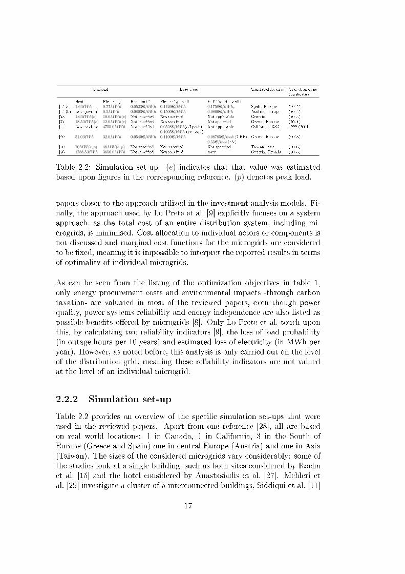
Demand Base Case Simulated location Year of analysis(publication)

Heat Electricity Heat tari� Electricity tari� FIT (feed-in tari�)[15](a) 1.6MWh 0.77MWh 0.0523e/kWh 0.1426e/kWh 0.1758e/kWhe Spain, Europe (2015)[15](b) Not speci�ed 0.5MWh 0.0803e/kWh 0.1500e/kWh 0.0800e/kWh Austria, Europe (2015)[28] 1.6MWh(e) 10.0MWh(e) Not speci�ed Not speci�ed Not applicable Generic (2013)[27] 18.5MWh(e) 12.0MWh(e) Not speci�ed Not speci�ed Not speci�ed Greece, Europe (2014)[11] Not speci�ed 4755.0MWh Not speci�ed 0.0528$/kWh(o�-peak) Not applicable California, USA 1999 (2004)

0.1005$/kWh (on-peak)[29] 51.0MWh 32.0MWh 0.0540e/kWh 0.1100e/kWh 0.08785e/kwh (CHP) Greece, Europe (2013)

0.55e/kwh(PV)[20] 70MW (e, p) 48MW (e, p) Not speci�ed Not speci�ed Not speci�ed Taiwan, Asia (2016)[26] 1788.5MWh 3650.0MWh Not speci�ed Not speci�ed none Ontario, Canada (2015)

Table 2.2: Simulation set-up. (e) indicates that that value was estimatedbased upon �gures in the corresponding reference. (p) denotes peak load.

papers closer to the approach utilized in the investment analysis models. Fi-nally, the approach used by Lo Prete et al. [9] explicitly focuses on a systemapproach, as the total cost of an entire distribution system, including mi-crogrids, is minimised. Cost allocation to individual actors or components isnot discussed and marginal cost functions for the microgrids are consideredto be �xed, meaning it is impossible to interpret the reported results in termsof optimality of individual microgrids.

As can be seen from the listing of the optimization objectives in table 1,only energy procurement costs and environmental impacts -through carbontaxation- are valuated in most of the reviewed papers, even though powerquality, power systems reliability and energy independence are also listed aspossible bene�ts o�ered by microgrids [8]. Only Lo Prete et al. touch uponthis, by calculating two reliability indicators [9], the loss of load probability(in outage hours per 10 years) and estimated loss of electricity (in MWh peryear). However, as noted before, this analysis is only carried out on the levelof the distribution grid, meaning these reliability indicators are not valuedat the level of an individual microgrid.

2.2.2 Simulation set-up

Table 2.2 provides an overview of the speci�c simulation set-ups that wereused in the reviewed papers. Apart from one reference [28], all are basedon real world locations: 1 in Canada, 1 in California, 3 in the South ofEurope (Greece and Spain) one in central Europe (Austria) and one in Asia(Taiwan). The sizes of the considered microgrids vary considerably: some ofthe studies look at a single building, such as both sites considered by Rochaet al. [15] and the hotel considered by Anastasiadis et al. [27]. Mehleri etal. [29] investigate a cluster of 5 interconnected buildings, Siddiqui et al. [11]

17

Wind Photovoltaic Conventional thermal CHP Gas boiler Electric Heat Electric storageturbine unit boiler storage

Cost R.p. Cost R.p. Cost R.p. Cost R.p. Cost R.p

[11] 8650$/kW 5 1730$/kW 25 1333$/kWe 30 1185$/kW 215 3960$/kW 2007450$/kW 20 970$/kW 55 (12.5) 936$/kW 500 (12.5)6675$/kW 50 833$/kw 100 (12.5)6675$/kW 100 1185$/kW 215

(20) 936$/kw 500(12.5)

[26] 3400$/kW 5000$/kW 3600$/kWe 60$/kW 60$/kW 132$/kWh(20) (20) (20) (16) (16) (5)

[27] No speci�c data reported; used Bailey et al. [25] as reference[29] 4305e/kWp 1583e/kWe 1 760e/kW 25e/kW

911e/kWe 5 (20) (10)835e/kWe 10653e/kWe 15650e/kWe 25

(20)[20] Uses data presented in [26]

Table 2.3: Technology capital cost (with assumed lifetime in years). �R.p.�stands for �Rated power�, in kW.

Wind Photovoltaic Conventional thermal CHP Gas boiler Electric Heat Electric storageturbine unit boiler storage storage

[11] 14.300$/kW 26.500$/kW 5.000$/kW 0.015$/kWh14.300$/kW +0.003g/kWh +0.015$/kwh12.000$/kW 7.500$/kwh11.000$/kW +0.015$/kwh

[15] No data reported[15] No data reported

+10$/startup[27] No data reported[28] No data reported[29] 12.3033e/kWp 0.027e/kWh 0.027e/kWh 0.001e/kWh

+0.015e/kWh[20] Uses data presented in [26]

Table 2.4: Technology yearly maintenance and operational costs.

look at a total of 69 interconnected sites, Yu et al. [20] consider an entireindustrial zone and lastly Zachar et al. [26] consider the energy needs of anentire town. This spread in sizes means that many possible sizes have beenconsidered, but it does also mean that the results can't be all that readilycompared to each other. Another factor that impedes easy comparison is thelarge spread on energy tari�s across the reviewed papers. Year of publica-tion, and when mentioned, the year considered for the simulation is reportedfor each paper as well, as the examined timeframe might impact both theenergy and technology prices. When no speci�c year for the simulation ismentioned in the reference, the year of publication is used. Table 2 showsthat all but one of the reviewed papers fall within a four-year period, from2013 to 2016, the exception being [11], with a simulation set in 1999.

Capital and operating costs are listed in tables 2.3 and 2.4 respectively. Ref-erence [11] in particular goes into much technical detail with regards to gen-

18

No additional policy Carbon Minimum Economic Emissions Minimum Time of use pricingintervention taxation autonomy incentives cap renewables

Macrogrid connected [9],[15],[26],[27],[20] [9],[11] [26],[20] [15],[26] [26] [26] [11],[28][15],[26] [27],[29][27],[28][29],[20]

Islanded operation ([26])Wind turbine [26],[20] [26] [26],[20] [26] [26] [26]Photovoltaic [9],[26],[27],[20] [9],[11] [26],[20] [15],[26] [26] [26] [11],[28]

[26],[27] [27],[29][29]

Conventional thermal unit [20] [11] [20]CHP [9],[26],[27],[20] [9],[11] [13],[26] [26],[27] [15] [26] [11],[28]

[15],[26] [29][27],[29]

Gas boiler [15],[26] [15],[26] [26] [26],[28] [26] [26] [28][29]

Electric boiler [26] [26] [26] [26][26] [26]Solar thermal [15]Storage (heat) [20] [29]

Storage (electric) [26],[20] [11],[26] [26],[20] [26],[27] [26] [26] ([11]),[28][27],[28]

Demand response [9] [15]

Table 2.5: Technology and policy matrix.

erating technologies, as discrete units are considered, each with their ownfuel e�ciencies and speci�c operational characteristics, which accounts forthe numerous entries in the tables. The other reviewed papers choose tolinearise the available generating technologies, meaning that generation andstorage capacity, if applicable, can be had in a continuous spectrum. Oneexception to this rule is the CHP in [26], where one �xed sized is considered.Higher installed CHP capacity is then achieved by installing multiples of thisunit. There is a rather large discrepancy between the costs for gas boilersbetween [26] on the one hand and [15, 29] on the other hand. It should how-ever also be noted that the heat demand considered in [26] is several ordersof magnitude greater than that in [15, 29], as shown in table 2.2. Where in-stallation and capital cost data is concerned, [27] directly refers to the workof Bailey et al. in [25]. However, in [25], various sizes and makes of eachtechnology option are discussed, while it is not clear which model is selectedin [27], meaning the installation costs in [27] remain unclear. In a similarvein, Yu et al. [20] reference Ren and Gao [26] for the speci�cs on the selectedequipment used in their model.

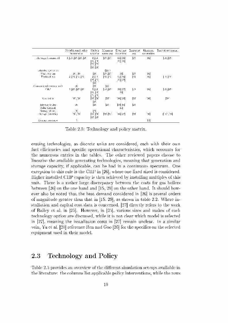
2.3 Technology and Policy

Table 2.5 provides an overview of the di�erent simulation set-ups available inthe literature: the columns list applicable policy interventions, while the rows

19

show which technologies were considered in the respective papers. While thereviewed papers usually simulated combinations of various technologies, it isimportant to note that possible policy interventions were mostly simulatedseparately, meaning that interaction e�ects are never explicitly investigated.In some cases, however, multiple policy interventions are present at the sametime, both [27] and [29] investigate the impact of carbon taxation, but againstthe very speci�c backdrop of a setting that highly favours PV through FIT.Additionally, the analysis conducted in [11] includes a time-of-use tari�, butthe impact of this tari� is never explicitly investigated. Aghaei & Alizadeh.in [28] approach the research problem from a di�erent direction: in their sim-ulation, there is both a carbon tax and real-time pricing, and three possibletechnology con�gurations are investigated against this backdrop.

2.3.1 Technologies

The working principles of the technologies listed in table 2.5 is outside thescope of this review. However, two important observations can be readilymade from this table: �rstly, most research attention is directed towards theelectrical side of a microgrid: only one publication looks at solar thermalpanels and one publication at heat storage. This does not mean that heatdemand is neglected: as evidenced by the inclusion of CHP in the majorityof reviewed papers, the total energy consumption of the microgrid is investig-ated. This focus on the electrical side of the microgrid does mean that thereare no analyses on the trade-o� between electrical and thermal storage, in allbut one paper only electrical storage is considered, while heat demand mustalways be instantaneously met. Secondly, while the ability to operate in is-landed mode is one of the frequently mentioned advantages of a microgrid,it is not one that has been subjected to any economic scrutiny.

2.3.2 Policy measures

While the selected technologies are self-explanatory, this is less the case wherethe researched policies are concerned. This section will therefore provide adiscussion of how the various policies have been implemented in the simula-tions being reviewed.

No additional policy measures

This is the business as usual alternative, and always used as a base casescenario, allowing for the impact of other policy interventions to be estimated.

20

Carbon taxation

As can be seen from table 5, this is the most researched policy intervention.As mentioned in section 2, methodology, the goal of this policy is to arrive atcarbon abatement through the internalisation of the societal costs associatedwith the emissions of CO2. It is important to note that both self-generatedelectricity, where applicable, and electricity bought from the grid are subjectto the emissions taxation, for grid-bought electricity, this is added as an extracharge on the electricity bill. Zachar et al. [26] investigate the impact of acarbon price of $30 per ton CO2, while in [27] a price ranging from e15 toe20 in increments of e0.5 per ton CO2 was considered. Siddiqui et al. in[11] investigate a wider price range: their simulations study a carbon priceranging from $0 to $1000 per ton in increments of $100 per ton. The scopesof [15],[29] are more limited when it comes to carbon taxation: [29] pricesemitted CO2 at e17 per ton and [15] investigates the impact of a carbon taxof e20 per ton of CO2. This shows that the consensus expected price forcarbon emissions is somewhere around e20 per ton, which is in line with theCommittee for Climate Change's predictions, forecasting a price of e20 perton by 2050 [27]. In [20], carbon taxation is investigated in a range centeredon $0.06, unfortunately, it is not mentioned per which amount of weight this$0.06 will be levied, making it di�cult to include the reported results in thecomparison presented below in a meaningful way.

Economic incentives

This is in itself a broader array of policy measures, as tax-related incentives,subsidies or bene�cial feed-in tari�s for �green� electricity are all possibilit-ies. Furthermore, these policies can also be targeted to a speci�c technology.Rocha et al. investigate the impact of a feed-in tari� of e0.1758/kWhe ande0.1812/kWhe for CHP and PV respectively [15]. In [26], tax incentivesamounting to 30% and 50% of the total installed cost of PV and wind en-ergy are investigated. No speci�c implementation of these tax incentivesis discussed, but for the purpose of the simulation, it su�ces that the ef-fect, regardless of implementation, is to reduce the overall cost of installingrenewable energy sources by the stated amount.

Time of use pricing

The impact of time of use pricing is investigated in [15],[28]: Aghaei & Aliz-adeh [28] opt for a real-time pricing scheme, with the price �uctuating on anhourly basis between $1.7/kWh and $4.2/kWh, according to a predeterminedscheme. Rocha et al. [15] study the e�ects of a time of use tari� structure

21

using time blocks: electricity is priced at e0.1601/kWh between 7:00 and14:00 as well as between 17:00 and 20:00, e0.1513/kWh between 14:00 and17:00, and e0.1405/kWh otherwise. The impact of other tari� systems onmicrogrid economics and optimal design is not investigated.

Command and control policies

As table 2.5 shows, only one paper researches the impact of various non-market based policies. As the three investigated polices are all quite similar inimplementation, they will be jointly discussed. Zachar et al. [26] investigatea level of minimum autonomy, to be understood as a minimum percentageof energy produced by local sources, a limit on the annual CO2 emissions,implemented as a percentage-wise reduction from a base case, and lastly aminimum percentage of power generated from local renewable sources. Eachtime, the policies are simulated in 5% increments between 0% and 100% of themandated policy. In order to facilitate a good understanding of the reviewedresults, it is important to note that Zachar et al. [26] have set up their workin such a way that this minimum autonomy is the base case to which theother policy interventions are compared, meaning that the optimal microgriddesign, given a certain policy intervention and a pre-determined autonomylevel is investigated. Yu et al. [20] only look at a minimum autonomy levelusing �ve distinct scenarios. Each scenario de�nes the minimum percentageof heat and power load that the microgrid is obliged to serve, starting from10% and progressing to 50% in 10% increments [20].

2.4 Reported results

This section will summarise the research results of the reviewed papers. Aftera discussion of the simulation results without policy interventions, the re-mainder of the reported results are grouped by policy intervention, allowingfor the expected outcomes of each policy intervention to be discussed.

2.4.1 Business as usual

Zachar et al. start their results with the results of an optimisation run withno constraints on installed technology, or required autonomy levels [26]. Theresults show that no microgrid technology is installed: all required power isbought from the macrogrid, and natural gas combustion in boilers is usedto ful�l heat demand. They also investigate a minimum autonomy require-ment, which is used as a base-case microgrid con�guration which serves as a

22

comparison for the microgrid con�gurations obtained under the consideredmarket based policies. CHP-units in combination with power purchases fromthe macro grid are used in this case, with token amounts of wind power (nevermore than 5% of total power generation) at the 40% and 80% autonomy scen-arios, as in each of those cases the installed CHP-units are working at fullcapacity. Additional CHP-units are installed at the 45% and 90% autonomylevels.

2.4.2 Carbon taxation

A �rst interesting result shared between a number of reviewed papers [11],[15], [26] is that carbon taxation at the expected level does not noticeablyimpact the technology selection of the microgrid. As a direct result, the car-bon taxation does not result in any signi�cant emission reduction comparedto the microgrid running without carbon taxation being present, meaningthe only real result is an increase of total energy costs for the microgrid. Thereason for this behaviour is that, at realistic carbon taxation levels of betweene15 to e25 per ton, the carbon price is simply too low to o�set the high cap-ital costs associated with carbon-free generation technologies such as windturbines and PV-panels. Siddiqui et al. [11] also investigate the impact of ahigher level of carbon taxation, and only when the price of carbon reaches$900 per ton does it incentivise the installation of PV-panels, according tothe results presented in [11]. Such a carbon price is however far above eventhe most pessimistic forecasts of the Interagency Working Group on SocialCost of Carbon, which prices the social cost of carbon in 2015 to be below$105 per ton with 97% certainty [28].The two papers reporting on simulations in a Greek setting however, havenoticeably di�erent results: both in the works by Anastasiadis et al. [27]and Mehleri et al. [29] the simulation results indicate the heavy adoptionof PV. This is however not in contradiction with the results reported byother authors, as the examined situation can be considered to be a fringecase, owning to the extremely favourable FIT for solar panels (0.55e/kWhas reported in [29]), meaning the high capital cost of PV-panels is stronglymitigated in such a setting. Even in these cases, CHP units are still part ofthe system, accounting for 23% of the installed capacity and supplying about50% of the energy demand in the microgrid in [29].Interestingly, Yu et al. [20] report outcomes that deviate from the resultsdiscussed above: their simulation results indicate that, for the case theyconsidered, the optimal system is made up of a balanced mix of internalcombustion engines and solar PV, with each accounting for half of the in-stalled capacity. Yu et al. attribute this to the fact that solar PV does not

23

require any fuel for operation, and the year-round sunny weather in the loc-ation they study [20]. No data is provided by Yu et al. in [20] on the amountof energy provided by the various technologies installed, and hence we haveno insight into the utilization of each of the retained technologies.

2.4.3 Economic incentives

The reviewed papers show that economic incentives can certainly have animpact on the economic optimal microgrid con�guration: Zachar et al. [26]investigate the impact of both a 30% and a 50% tax credit towards renewableenergy investments. Their results show a rather limited impact for a 30%tax credit, but a far more appreciable impact for a 50% tax credit: in thecase of a 30% tax credit only a token amount of energy is procured fromwind power, never surpassing more than 5% of total energy supply. A taxcredit amounting to 50% of investment cost for renewable energy howeverincentivises the adoption of wind power a lot more: not only does it delaythe installation of a �rst CHP-unit until 20% local autonomy is demanded,this level of tax credit also assures that up to one third of the total powergeneration is sourced from renewable sources. It should be noted that theadoption percentage of renewables under this scenario is not monotonouslyincreasing with the requested autonomy, it is rather dependent on the num-ber of CHP-units installed, and shows a jump downwards whenever an addi-tional CHP-unit is installed. However, even under a 50% tax credit scheme,CHP-units still contribute the dominant share of locally generated power tothe microgrid, except at the 5% to 15% autonomy levels, where only windpower is installed. The impact on emissions of a tax credit is reported tobe once again dependent on the height of the tax credit, with only a 50%tax credit being able to motivate microgrids to achieve meaningful emissionreductions of between 5% and 25% of emission when compared to the buyall from macrogrid scenario, depending on the desired autonomy level. Thereviewed papers which research the e�ects of FIT's are unanimous in their�ndings: in the papers where the con�guration of the generating capacityis optimised, the technology favoured by the FIT is adopted: in [29] PVis installed up to the maximum allowable capacity (10 kW per building) asde�ned by legislation. In [15], set systems con�gurations are tested, but thee�ect of the FIT is more dependent on the height of the FIT in comparisonto the electricity rate: when the FIT is higher than the purchase price ofelectricity, all locally generated electricity is sold back to the macrogrid, andall the required power is bought from the macrogrid. When the line lossesthis incurs are considered, this is clearly a suboptimal solution.

24

2.4.4 Tari� systems

Rocha et al. �nd that switching to a TOU-tari� has negligible impact ontheir obtained results [15]. Aghaei & Alizadeh [28] �nd that the impact ofreal-time pricing combined with carbon taxation works in two directions:under such a scheme generation costs fall when demand response and energystorage are implemented in a CHP-powered microgrid, while emission costsrise. When only energy storage is incorporated, however, energy costs riseslightly while emission costs rise even higher, showing that energy storage isin itself not economically viable.

2.4.5 Command and control policies

Zachar et al. [26] show that both an emissions cap scenario or a minimumrenewable scenario are the most e�ective ways to mitigate carbon emissions.As can be expected, an emission cap scenario is most e�ective at cappingemissions at a selected target level. However, this comes at a steep cost tothe microgrid: total energy procurement costs are double those of the refer-ence scenario at 50% emissions reductions, and rise to seven times the costof the reference scenario at 100% of emissions reduction. This is also theonly scenario investigated by Zachar et al. [26] where the amount of powerfrom CHP-units decreases as the investigated scenario variable, i.e. emissionreduction, goes up: at 5% emissions reduction, 30% of the required power isgenerated by CHP while the rest is bought from the macrogrid. Renewablesintegration starts at 10% emissions reduction, with the installation of 5% ofwind power, and renewables become the dominant power source at a man-dated emission reduction of 45%.

The minimum renewables scenario of Zachar et al. [26] is the only set-upof all the reviewed papers where the result of the optimisation does notinclude CHP-units. In this scenario, all the power generated by the microgridwill originate from renewable sources. This also means that the emissionsassociated with the energy consumption of the microgrid fall at a steady paceas the minimum percentage of renewables is increased. As was the case withthe previously discussed command and control intervention, this too comesat a cost for the microgrid, as costs quickly rise when compared to the basecase.

25

2.5 Discussion

This section discusses the reported �ndings in the literature. A �rst partof the discussion aims to synthesize the above reported results into gen-eral trends concerning both the considered technologies and policy measures,while a second part delves more deeply into recommendations for furtherresearch.

When reviewing the results reported in the literature, it is immediately ap-parent that the scienti�c consensus strongly favours the adoption of CHP-units in microgrids: not only are they included in all but one of the optimalsolutions of each of the reviewed problems, CHP-units are also the mostprominent energy provider in the microgrid. The reason for this is alwaysthe high capital costs associated with renewable energy generation technolo-gies. This means that the often-heard bene�t of microgrids, enabling greaterintegration of renewable energy sources, is not really supported by the eco-nomic analyses that have been carried out, as renewable energy sources onlybecome economically attractive when they are heavily favoured by policymeasures, either through market based interventions such as tax credits orgenerous FIT's, or through non-market based command and control policiesby the imposition of an emission cap or a minimum renewable requirementwhen it comes to power generation.

This favoured adoption of CHP-based microgrids is also stable through time,as CHP-units are part of the solution found for 1999 by Siddiqui et al. [11]as well as being the staple in the optimal solution reported on in 2015 byZachar et al. in [26]. Considered against the backdrop of the price of PV-panels which fell by 80% over the considered timespan [29], this seems toindicate that there are other barriers to the adoption of PV-systems in mi-crogrids in addition to the signi�cant capital costs associated with installingPV-panels. This conclusion is further substantiated by the observation thatPV-panels are only installed on a large scale in those scenarios where they arespeci�cally targeted by policy measures. Such measures can bias the choicesavailable to actors, e.g. generous feed-in tari�s for electricity produced byPV-systems as was the case in [10]. Alternatively, such policy measures canrestrict the choices available to actors, such as a mandated emissions reduc-tion, or an obligatory minimum stake of renewables, both investigated in [26].

Electricity from wind turbines is investigated in only two of the reviewedpapers [26],[20]. This is not exactly surprising, since wind turbines o�er toomuch generation capacity to be considered for inclusion in most microgrids,

26

which explains why they were included in [26], as this was by far the largestmicrogrid, encompassing an entire town. Based on the reported results, windturbines prove themselves to be the more economically viable renewable elec-tricity source when compared to PV-panels. This means that the sizing of amicrogrid is possibly not as straightforward as it seems: in all the reviewedpapers, the considered microgrids are of �xed size, with the heat and powerdemands being treated as givens. However, the reported results in [26] withregards to the adoption of wind turbines indicates that there are possiblyeconomies of scale waiting to be realised. The �ndings reported in [20] seemto contradict the results of Zachar et al. [26] as no wind turbines are part ofthe reported solution. However, Yu et al. [20] report that the reason behindthe non-inclusion of wind turbines is that the local wind speeds at locationconsidered were too low.

The unattractiveness of renewables from a purely economic standpoint isclearly shown by Zachar et al. in [26], as the total costs for the microgridincrease the more the adoption of renewables within the microgrid is enforcedthrough government intervention. These costs are not as readily apparent inthe scenarios using FIT's or tax incentives due to the scope of the analyses:the focus is always on the costs and bene�ts accrued by the owner or operatorof the microgrid, while in these scenarios, the costs of the adoption of renew-able energy sources will be borne by society as a whole through levies or taxes.

The observation that CHP-units will only be replaced by renewable energysources if the carbon prices were to rise far above the expected societal costsof carbon means that from a purely economic point of view, it is better to con-tinue to burn fossil fuels while compensating the damage to society throughpayment of a carbon tax, than to switch to renewable energy generation,considering the current state of technology and the current estimates of thesocietal costs of carbon. Additionally, the amount of emission reductionsrealised by the adoption of CHP-powered microgrid is highly dependent onthe energy mix used to power the macrogrid, indicating that the expectedenvironmental impact of microgrid adoption remains unclear.

It is also interesting to note that the discussion of the environmental impactsdue to the generation of electricity is narrowed to the emission of carbon,which is then remedied via carbon taxation. However, the generation of elec-trical energy also has other potential externalities on human health [30], suchas the emmissions of other greenhouse gasses such as CH4 and N2O or airpollutants such as SO2 or NO2. Work has been done on trying to determinethe costs of these externalities by Shindell in [31] and it stands to reason that

27

the inclusion of these costs in a way analogous to carbon taxation would fur-ther promote the use of more environmentally friendly electricity generationoptions. Such a measure would also mean that renewable generation wouldbe competitive at comparatively lower levels of carbon taxation.

From a policy perspective, the rather sobering conclusion is that carbontaxation, the most researched and technology neutral policy intervention,seems to have at best a minor impact on the optimal system con�gurationof microgrids, with its e�ects mostly being limited to increasing the total en-ergy procurement cost for the microgrid. However, targeted interventions toboost adoption of one particular technology over the other are also e�ective,as proven by adoption of solar panels in the reviewed Greek settings. Moreheavy-handed interventions, such as obligatory emissions reductions are alsoproven to be e�ective in steering the system con�guration of microgrids to-wards renewable energy sources, but this is accompanied by a large increasein private costs, casting doubt upon the feasibility of such measures.

The parameters on which microgrids are evaluated in the reviewed papers,are rather narrow: only the total or operational energy procurement costsand carbon emissions are considered. Lo Prete et al. [9] [9] for instanceshow that the adoption of microgrids representing 8% of total generation ca-pacity would lead to an increase of 30% in reliability of the entire electricalnetwork. This shows that microgrids can certainly o�er bene�ts where reliab-ility is concerned. However, these bene�ts are neither valued nor investigatedat the level of an individual microgrid by the reviewed papers, meaning theadoption of microgrid technology is possibly undervalued. This is clearly apromising avenue of further research.

Additionally, the impact of di�erent tari�s systems is not investigated in thereviewed papers, especially considering that a restructuring of the currenttari� system might incentivise some behaviour while penalising other beha-viours. See for example Schreiber et al. [20] for a discussion on a capacitypricing model: the tari�s they design are not linked to the time of day whenenergy is required from the grid, but rather what the peak withdrawal poweris. Their approach is exclusively focussed on the electricity component ofenergy demand, and takes a system view, choosing not to focus on the in-dividual microgrid level. While therefore their work is outside the scope ofthis review paper, it is still relevant in that it shows that tari�s can be usedto steer the behaviour of connected consumers in certain directions. Giventhis e�ect of tari�s, it stands to reason that a novel tari� system could haverepercussions on the optimal design of microgrids; this is however an area

28

that has not received any research attention up until now.

From a methodological point of view, we would like to recommend that fu-ture studies all include a baseline case, both with regards to the adoptionof microgrid technologies and the proposed policy interventions. Where mi-crogrid technologies are concerned, a baseline scenario would allow for a clearcost-bene�t analysis to decide whether or not the adoption of a microgridis economically viable. When it comes to policy analysis, the presence of abaseline scenario would greatly facilitate impact assessment of the consideredpolicies, as it would enable �before and after� discussions.

Additionally, we would recommend that future studies report all relevantdata used to produce the results, including not only equipment installationand maintenance costs, energy tari�s and taxation levels, but also inform-ation relating to the heat and power demand of the considered microgridas well as the rated heat and power capacities of the selected technologies.Such disclosure would greatly help in allowing the reproduction of reportedresults, allow for the assessment of the impact of changes in technology costsor tari�s and even enable the investigation of parameters, such as microgridsize which have remained uninvestigated up until now.

2.6 Conclusion

In this paper, we have reviewed the current research literature concerningthe impact of policy measures on the economically optimal con�guration ofmicrogrids. With regards to the �rst goal of this review paper, outlining thecurrent state of the art in research surrounding the economics of microgrids,we have shown that the methodology of choice is the minimisation of oper-ational or lifetime costs associated with the operation of the microgrid, de-pending on the time horizon. The used optimisation models in the literatureare similar both in objective function and in decision variables. The currentavailable literature on the impact of policy measures on the economicallyoptimal con�guration of microgrids considers microgrid sizes ranging fromsingle buildings up to entire communities, but without explicitly controllingfor the e�ects of microgrid size on the reported results. When it comes tothe investigated policy measures in the literature, it is apparent that a lotof research attention has been devoted to the topics of carbon taxation andTOU-tari�s, with other subjects such as tax incentives or command andcontrol policies only receiving moderate research attention. Furthermore,concerning the objective of outlining any research gaps, we have shown that

29

the exploration of the impact of tari� systems other than TOU-pricing onthe optimal con�guration of a microgrid hasn't received research attention upuntil now, making this an interesting avenue for further research. Our mostsigni�cant �nding is that, where the most often viable reported system con-�guration is concerned, the current scienti�c consensus is that CHP-poweredmicrogrids are the most economically viable type of microgrid under a widerange of policy interventions, with renewable powered microgrids only viablein fringe cases, making the often-heard claim that microgrids will allow forgreater penetration of renewable sources highly suspect at best.

Acknowledgements

We thank Prof dr. Theodoros Zachariadis for his suggestion that we alsoconsider externalities other than carbon emissions.

30

Bibliography

[1] Ringler P, Keles D, Fichtner W. Agent-based modelling and simulationof smart electricity grids and markets � A literature review. Renew andSustain Energy Rev 2016 May;57;205-15.

[2] Connor PM, Baker PE, Xenias D, Balta-Ozkan N, Axon CJ, CipciganL. Policy and regulation for smart grids in the United Kingdom. Renewand Sustain Energy Rev 2014 December;40;269-86.

[3] Allan G, Eromenko I, Gilmartin M, Kockar I, McGregor P. The eco-nomics of distributed energy generation: A literature review. Renewand Sustain Energy Rev 2015 February;42;543-56.

[4] Moretti M, Njakou Djomo S, Azadi H, May K, De Vos K, Van PasselS, et al. A systematic review of environmental and economic impacts ofsmart grids. Renew and Sustain Energy Rev; Forthcoming 2016.

[5] Moreno-Munoz A, Bellido-Outeirino FJ, Siano P, Gomez-Nieto MA. Mo-bile social media for smart grids customer engagement: Emerging trendsand challenges. Renew and Sustain Energy Rev 2016 January;53;1611-6

[6] Lasseter R, Akhil A, Marnay C, Stevens J, Dagle J, Guttromson R, etal. Integration of Distributed Energy Resources: The CERTS MicroGridConcept. White paper. Prepared for U.S. Department of Energy;2002.

[7] Lidula NW, Rajapakse AD. Microgrids research: A review of experi-mental microgrids and test systems. Renew and Sustain Energy Rev2011 January;15;186-202.

[8] Palizban O, K Kauhaniemi K, Guerrero JM. Microgrids in active net-work management�Part I: Hierarchical control, energy storage, virtualpower plants, and market participation. Renew and Sustain Energy Rev2014 August;36;428-39.

31

[9] Lo Prete C, Hobbs BF, Norman CS, Cano-Andrade S, Fuentes A, vonSpakovsky MR, et al. Sustainability and reliability assessment of mi-crogrids in a regional electricity market. Energy 2010 May;41; 192-202.

[10] IEEE Smartgrid [Internet]IEEE joint task force on quadrenniel en-ergy review, Utility and Other Energy Company Business CaseIssues Related to Microgrids and Distributed Generation (DG),Especially Rooftop Photovoltaics, Presentation to the U.S. De-partment of Energy 2014, [cited 2016 July 2016]. Availablefrom https://smartgrid.ieee.org/images/files/pdf/IEEE\_QER\

_Microgrids\_October\_3\_2014.pdf

[11] Siddiqui A, Marnay C, Edwards JL, Firestone R, Ghosh S, Stadler M.E�ects of a Carbon Tax on Microgrid Combined Heat and Power Adop-tion. J of Energy Eng. 2005 April;131;2-25.

[12] Bustos C, Watts D. Novel methodology for microgrids in isolatedcommunities: Electricity cost-coverage trade-o� with 3-stage techno-logy mix, dispatch & con�guration optimizations. Appl Energy 2017March;195;204-221.

[13] Prehoda E W, Schelly C, Pearce J M. U.S. strategic solar photovoltaic-powered microgrid deployment for enhanced national security. Renewand Sustain Energy Rev 2017 October;78;167-175.

[14] Coelho V N, Coelho I M, Coelho B N, de Oliveira G C, Barbosa A C,Pereira L, et al. A communitarian microgrid storage planning systeminside the scope of a smart city. Appl Energy 2016 http://dx.doi.

org/10.1016/j.apenergy.2016.12.043

[15] Rocha P, Siddiqui A, Stadler M. Improving energy e�ciency via smartbuilding energy management systems: a comparison with policy meas-ures. Energy and Build 2105 February;88;203-13.

[16] Zachar, M, Trifkovic M, Daoutidis P. Policy e�ects on microgrid eco-nomics, technology selection, and environmental impact. Comput andChem Eng 2015 October;81;364-75.

[17] Anastasiadis AG, Vokas G, Papageorgas P, Kondylis G, Kasmas S. Ef-fects of carbon Taxation, Distributed Generation and Electricity StorageTechnologies on a Microgrid. Energy Procedia 2014;50; 824-31.

[18] Aghaei J, Alizadeh MI, Multi-objective self-schedulingof CHP (com-bined heat and power)-based microgrids considering demand response

32

programs and ESSs (energy storage systems). Energy 2013 June;55;1044-54.

[19] Mehleri ED, Sarimveis H, Markatos NC, Papageorgiou LG. Optimaldesign and operation of distributed energy systems: Application to greekresidential sector. Renew Energy 2013 March;51;331-42.

[20] Yu N, Kang J-S, Chang C-C, Lee T-L, Lee D-Y. Robust economicoptimization and environmental policy analysis for microgrid plan-ning: An application to Taichung Industrial Park, Taiwan. Energy 2016October;113;671-682.

[21] Schreiber M, Wainstein ME, Hochlo� P, Dargaville R. Flexible electri-city tari�s: Power and energy price signals designed for a smarter grid.Energy 2015; 93;2568-2581.

[22] Mariam L, Basu M, Conlon M F. Microgrid: Architecture, policy andfuture trends. Renew and Sustain Energy Rev 2016 October;64;477-489.

[23] Martin-Martines F, Sánchez-Miralles A, Rivier M. A literature review ofMicrogrids: A functional layer based classi�cation. Renew and SustainEnergy Rev 2016 October;64;1133-1153.

[24] Dantzig, G B. Discrete-Variable Extremum Problems. Operations Re-search 1957;5(2);266-277.

[25] Bailey O, Ouaglal B, Bartholomew E, Marnay C, Bourassa N. AnEngineering-Economic Analysis of Combined Heat and Power Techno-logies in a µGrid Application., Ernest Orlando Lawrence Berkeley Na-tional Laboratory 2002, LBNL-50023 Prepared for the United StatesEnvironmental Protection Agency.

[26] Ren H, Gao W. A MILP model for integrated plan and evaluation ofdistributed energy systems. Appl Energy 2010;87:1001-1014.

[27] Committee on Climate Change, Meeting Carbon Budgets � the needfor a step change, First progress report 2009.

[28] Interagency Working Group on Social Cost of Carbon, Technical Sup-port Document: Technical Update of the Social Cost of Carbon for Reg-ulatory Impact Analysis Under Executive Order 12866, United StatesGovernment, 2013, rev. 2015.

33

[29] Feldman D, Barbose G, Margolis R, Bolinger M, Chung D, Fu R, etal. [Internet] Photovoltaic System Pricing Trends. Sunshot � USDepartment of Energy, 2015 (updated 2015 August 26; cited 2016July 7). Available from: https://emp.lbl.gov:/sites/all/files/

pv\_system\_pricing\_trends\_presentation\_0.pdf.

[30] European Commission (1995), ExternE: Externalities of Energy, O�cefor O�cial Publications of the European Communities, Luxembourg.

[31] Shindell (2013) D T. The Social Cost of Atmospheric Release. EconDiscuss Pap, No 2013-56, Kiel Institute for the World Economy.

34

Chapter 3

Economical optimization of

micorgrids: a non-causal model1

Abstract

In this paper we present an economical optimization model for a microgridconnected to the general electricity grid by minimizing the total operatingcost over a given period in the presence of uncertain future grid electricityprices. The microgrid is modeled to consist of �ve distinct blocks, four ofwhich make up the microgrid and the �fth one being the connection to thegeneral electricity grid. Each of these components has various adjustableattributes, allowing for the simulation of di�erent kinds of consumers as wellas di�erent storage and generation technologies. Consumption and intermit-tent generation are exogenous variables derived from existing datasets. Underuncertain future grid electricity prices, the storage component introduces anon-causal dependency into the model, to cope with this non-causality, wepresent various storage use strategies and analyze the resulting cost patternsusing real electricity price data and Monte Carlo simulations.

1This chapter has been published as Milis K., Peremans H. Economical optimization

of micorgrids: a non-causal model, PROCEEDINGS OF ASME 9TH INTERNATIONAL

CONFERENCE ON ENERGY SUSTAINABILITY, 2015, VOL 2

35

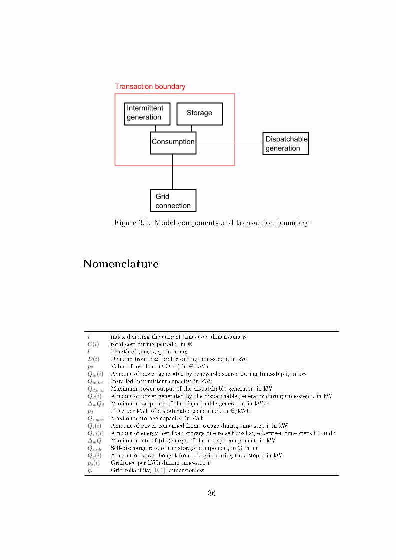
Intermittent generation

Storage

Consumption Dispatchable generation

Grid connection

Transaction boundary

Figure 3.1: Model components and transaction boundary

Nomenclature

i index denoting the current time-step, dimensionlessC(i) total cost during period i, in el Length of time-step, in hoursD(i) Demand from load pro�le during time-step i, in kWp∗ Value of lost load (VOLL) in e/kWhQin(i) Amount of power generated by renewable source during time-step i, in kWQin,tot Installed intermittent capacity, in kWpQd,max Maximum power output of the dispatchable generator, in kWQd(i) Amount of power generated by the dispatchable generator during time-step i, in kW∆mQd Maximum ramp rate of the dispatchable generator, in kW/hpd Price per kWh of dispatchable generation, in e/kWhQs,max Maximum storage capacity, in kWhQs(i) Amount of power consumed from storage during time-step i, in kWQs,l(i) Amount of energy lost from storage due to self-discharge between time-steps i-1 and i∆mQ Maximum rate of (dis)charge of the storage component, in kWQs,sdr Self-discharge rate of the storage component, in %/hourQg(i) Amount of power bought from the grid during time-step i, in kWpg(i) Gridprice per kWh during time-step igr Grid reliability, [0, 1], dimensionless

36

3.1 Introduction

A microgrid2 is a smaller scale electrical network, a copy of the full-�edgedelectrical grid in that it comprises electricity and thermal generation, con-sumption and storage, and that it has the capability to work in a self-contained manner, operating independently from the wider electrical grid [1].As this means that a microgrid must be able to monitor and control bothelectrical generation, storage and consumption to ensure that the microgridremains balanced at all times, it is easy to see how microgrids are part ofthe larger domain of smart grids [2]. In this paper we present an economicaloptimization model for a microgrid connected to the general electricity gridby minimizing the total operating cost over a given period in the presence ofuncertain future grid electricity prices.

To this end, the microgrid is modeled to consist of �ve distinct blocks, fourof which make up the microgrid and the �fth one being the connection tothe general electricity grid. The microgrid itself comprises a consumptioncomponent, a storage component and two local generation components, onemodeling intermittent generation while the other models dispatchable gener-ation. Each of these components has various adjustable attributes, allowingfor the simulation of di�erent kinds of consumers as well as di�erent storageand generation technologies. Consumption and intermittent generation areexogenous variables derived from existing datasets.

The decision variables in the discussed minimization model are the quantit-ies of power procured from the three power sources as well as the quantitystored in or removed from the storage component, constrained by maximumramp rates and the maximum capacity of the storage component. This isquite a well-studied problem, but up until present, only some work has beendone on micro grid under uncertainty. Most of the previous work uses ap-proximate methods in order to deal with the uncertainties of electricity price,intermittent generation and load associated with operating a microgrid [3-6]. These approximate methods use a probability based estimation of theuncertain variables, which is then used to optimize the unit commitment ofthe model components. This approach allows the side-stepping of compu-tationally expensive simulations, as it allows the optimization to be carriedout based on only a few statistical moments of the observed distribution.Our work, however, is more in line with [7], as we have chosen to use the

2See chapter 2 for a complete de�nition of a microgrid, only the parts relevant for the

discussion in this chapter are reprinted here.

37

Monte Carlo simulation approach. While this approach is more computa-tionally expensive, it allows us to gain a better appraisal and understandingof the underlying complexity and system behaviour, warranting the extracomputational time needed. In this paper we present a simple, yet robustframework for economic analysis of microgrids under a wide range of uncer-tainties; contrary to [7], not only uncertainty in intermittent generation, butalso uncertainty in electricity price, grid availability and electricity demand isaccomodated for. Under uncertain future grid electricity prices, the storagecomponent introduces a non-causal dependency into the model: the optimalquantity of electricity to keep in storage at any given moment depends onall future grid electricity prices. To cope with this non-causality, we presentvarious storage use strategies and analyze the resulting cost patterns. As itis important to mirror real electricity price conditions as closely as possible,historical price data are used. We present Monte Carlo simulations, by in-troducing small perturbations on historical price data, to investigate whichone of the di�erent storage use strategies, on average, minimizes cost and toinvestigate the price sensitivity of the di�erent strategies.

It is important to note that the focus of this research is on the econom-ics associated with operating a microgrid when confronted with uncertainelectricity prices, the consequence being that abstraction is made of many, ifnot all of the electro-technical intricacies accompanying microgrid operation.Furthermore, although microgrids commonly include heat as well as electri-city, for the remainder of this paper, the focus is solely on the electrical side.

The next section provides an overview of the model and the various includedcomponents, after which the cost function is discussed. A following sectiondetails three di�erent storage use strategies, which serve as a basis for thesimulation presented in the penultimate section. A �nal conclusion closesthis paper.

3.2 Model overview and components

To simulate a microgrid, a model is built using Matlab. Matlab has beenchosen as development environment because of relative ease of use and be-cause the main focus of the modelling e�ort is both on system dynamic andeconomic behaviour, not on electro technical intricacies of microgrid opera-tion. Matlab provides the �exibility to explore both areas of interest, whileavoiding the technical details often associated with software packages spe-cialised in modelling electrical systems. In the interest of keeping model

38

complexity as low as possible, the model was build using only Matlab, andthe decision to forgo the use of Simulink or other Matlab tool kits was made.A visualisation of the model described here can be found in Fig. 3.1.

Consumption

The �rst component of the model is the consumption block. This blockcontains the load pro�le, modelling the consumption of electricity through-out the day. This load pro�le can be completely �xed, simulating a normalpresent-day consumer of electricity, or demand response can be integrated,meaning that electricity consumption can be cut back or shifted to othermoments in times of high electricity prices (in the case of a grid-connectedconsumer) or in times of insu�cient generation capacity to serve all loads.It is important to note however, that not all load can be shifted or reducedat will, as there will always be a residual base load which must be met: forindustrial consumers this base load is driven by economic activity, while forhouseholds it is easy to envisage that certain electricity-supplied amenities,such as lighting during mornings and evenings, are non-negotiable. As canbe surmised from the above discussion, it is the intention of the model to beable to simulate residential, commercial and industrial electricity consumersby adjusting the used load pro�le, both in total electricity demand and tim-ing of the load peaks. A load pro�le is not generated while the model runs,but is supplied from externally available data to the model as an input.

Intermittent Source

The second component models a distributed intermittent electricity source: awind turbine, solar panels, or a combination of both. The choice of modelingsolar or wind energy will be re�ected in the generation pro�le. The modelingof both of these is a �eld of scienti�c study in and of itself, but there arepublicly available datasets which will be used. While all of the other genera-tion components have both a variable and �xed cost, the intermittent powersource is assumed to have only a �xed installation cost. The reason why novariable cost component is included is that the marginal cost of producing anextra kW of electricity using an intermittent renewable source is zero: oncethe wind turbine or solar panels are installed there is no extra cost to produceelectricity once the wind is blowing or the sun is shining. This also meansthat the intermittent power source receives preferential treatment: when itis available, its full output at that moment will always be used.

39

Local Dispatchable Power

The next model component simulates locally available dispatchable powergeneration, for instance a diesel generator or gas turbine. To accuratelymodel such a generation unit, a set of parameters will be used, split into twocategories: on the one hand technical parameters, namely maximum poweroutput and ramp rate -the maximum percentage change in output per modelstep- and on the other hand cost parameters consisting of a variable cost perkW produced and a �xed installation cost. By setting these parameters toappropriate values, di�erent generation technologies can be modeled.

Storage

Another model component is the electrical storage component. Like the dis-patchable generation component, this component is modeled using a numberof parameters enabling the simulation of di�erent storage technologies, suchas battery storage, pumped hydro, fuel cells or supercapacitor storage. Onceagain, the parameters can be classed as technical parameters, which are totalstorage capacity, maximum rate of charge and discharge and rate of self dis-charge on the one hand and a �xed cost parameter on the other hand.

Grid Connection

The �nal model component is the grid connection. This component functionsas a limitless source and sink as an unconstrained amount of power can bebought from or sold to the grid during each simulation step. Like previousmodel components, the grid connection has cost related parameters: it ismodeled using a variable cost per kWh electricity bought, a �xed intercon-nection cost, and a variable bene�t per kWh electricity sold. In addition toall these, the grid connection is also modeled as having a certain reliability,meaning that there is a probability at each time-step that the grid will notbe available to the microgrid user.

Transaction Boundary

Not a component as such, but also present in Fig. 3.1 is the transactionboundary: only energy �ows passing this boundary will generate costs or

40

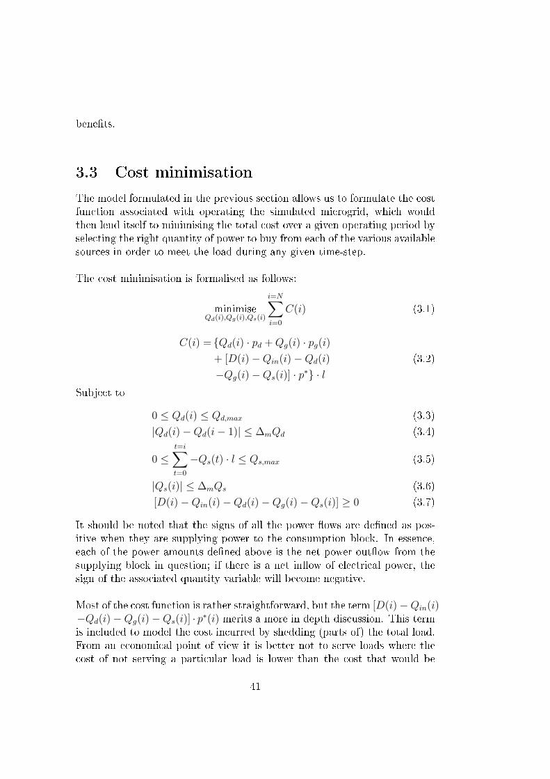
bene�ts.

3.3 Cost minimisation

The model formulated in the previous section allows us to formulate the costfunction associated with operating the simulated microgrid, which wouldthen lend itself to minimising the total cost over a given operating period byselecting the right quantity of power to buy from each of the various availablesources in order to meet the load during any given time-step.

The cost minimisation is formalised as follows:

minimiseQd(i),Qg(i),Qs(i)

i=N∑i=0

C(i) (3.1)

C(i) = {Qd(i) · pd +Qg(i) · pg(i)+ [D(i)−Qin(i)−Qd(i)

−Qg(i)−Qs(i)] · p∗} · l(3.2)

Subject to

0 ≤ Qd(i) ≤ Qd,max (3.3)

|Qd(i)−Qd(i− 1)| ≤ ∆mQd (3.4)

0 ≤t=i∑t=0

−Qs(t) · l ≤ Qs,max (3.5)

|Qs(i)| ≤ ∆mQs (3.6)

[D(i)−Qin(i)−Qd(i)−Qg(i)−Qs(i)] ≥ 0 (3.7)

It should be noted that the signs of all the power �ows are de�ned as pos-itive when they are supplying power to the consumption block. In essence,each of the power amounts de�ned above is the net power out�ow from thesupplying block in question; if there is a net in�ow of electrical power, thesign of the associated quantity variable will become negative.

Most of the cost function is rather straightforward, but the term [D(i)−Qin(i)−Qd(i)−Qg(i)−Qs(i)] · p∗(i) merits a more in depth discussion. This termis included to model the cost incurred by shedding (parts of) the total load.From an economical point of view it is better not to serve loads where thecost of not serving a particular load is lower than the cost that would be

41

incurred when serving said load. This term can never be negative: whilethe residual demand or the di�erence between total demand and the amountof power provided by the intermittent source might become negative, thisexcess power will always either be stored or sold to the grid. It is howeverpossible for this term to be positive; this would mean that there is excessdemand for electrical power which can not be met. Should this situationarise, excess load will have to be shed, incurring p∗ as a cost, representingthe value of the lost, or shed, load. Constraint (7) makes sure that the modeladheres to the line of reasoning outlined above.

The energy �ows from the dispatchable generator and from the storage havetwo constraints each. Constraint (3) stipulates that the energy �ow from thegenerator must at all times be positive -so energy in�ows into the generatorare not possible- and has the maximum rated generation capacity as an upperbound, while constraint (4) is formulation of the maximum ramp rate of thedispatchable generator. Constraint (5) states that the storage unit cannotcontain more than its maximum capacity, and also that it is impossible atany given time to store less than zero kWh, which in e�ect means that nomore power can be obtained from the storage component when this last oneis empty. Constraint (6) states that the energy �ow to the storage componentis bounded by the maximum rate of charge and maximum rate of discharge.

In order to model as many di�erent scenarios as possible, pg(i) can havea di�erent value depending on the sign of Qg(i); this is to account for situ-ations where there is a di�erence between the price of electricity bought fromthe grid and the price for selling electricity to the grid.

It is worthwhile to point out that, even though there is no price compon-ent attached to energy entering or leaving the storage component, the costsand bene�ts associated with this �ow are however accounted for. If the storedenergy originates from the intermittent source, it is assumed to be free asdiscussed earlier and in the case it originates from either the grid or thedispatchable generation, it has accrued costs when it crossed the transac-tion boundary from either of those sources. In a similar vein, energy leavingstorage will only generate a bene�t when it is sold to the grid and crossesthe transaction boundary. When stored electricity is consumed, no bene�tis generated, but this will nevertheless impact the overall costs by avoidingthe procurement of this quantity of electricity from either the grid or the dis-patchable generator. Similarly, energy lost from storage due to self-dischargedoesn't generate costs when it leaks from storage, but generates costs whenit is procured from the grid or the dispatchable generation; leakage losses will

42

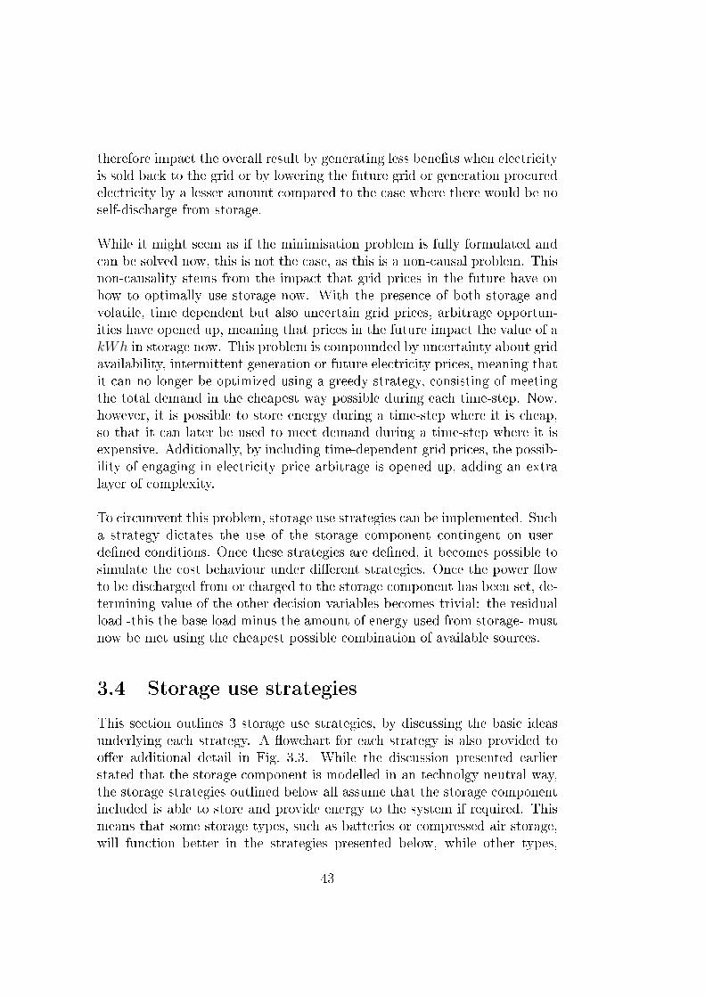
therefore impact the overall result by generating less bene�ts when electricityis sold back to the grid or by lowering the future grid or generation procuredelectricity by a lesser amount compared to the case where there would be noself-discharge from storage.

While it might seem as if the minimisation problem is fully formulated andcan be solved now, this is not the case, as this is a non-causal problem. Thisnon-causality stems from the impact that grid prices in the future have onhow to optimally use storage now. With the presence of both storage andvolatile, time dependent but also uncertain grid prices, arbitrage opportun-ities have opened up, meaning that prices in the future impact the value of akWh in storage now. This problem is compounded by uncertainty about gridavailability, intermittent generation or future electricity prices, meaning thatit can no longer be optimized using a greedy strategy, consisting of meetingthe total demand in the cheapest way possible during each time-step. Now,however, it is possible to store energy during a time-step where it is cheap,so that it can later be used to meet demand during a time-step where it isexpensive. Additionally, by including time-dependent grid prices, the possib-ility of engaging in electricity price arbitrage is opened up, adding an extralayer of complexity.

To circumvent this problem, storage use strategies can be implemented. Sucha strategy dictates the use of the storage component contingent on user-de�ned conditions. Once these strategies are de�ned, it becomes possible tosimulate the cost behaviour under di�erent strategies. Once the power �owto be discharged from or charged to the storage component has been set, de-termining value of the other decision variables becomes trivial: the residualload -this the base load minus the amount of energy used from storage- mustnow be met using the cheapest possible combination of available sources.

3.4 Storage use strategies

This section outlines 3 storage use strategies, by discussing the basic ideasunderlying each strategy. A �owchart for each strategy is also provided too�er additional detail in Fig. 3.3. While the discussion presented earlierstated that the storage component is modelled in an technolgy neutral way,the storage strategies outlined below all assume that the storage componentincluded is able to store and provide energy to the system if required. Thismeans that some storage types, such as batteries or compressed air storage,will function better in the strategies presented below, while other types,

43

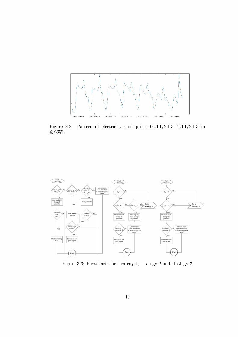
Figure 3.2: Pattern of electricity spot prices 06/01/2013-12/01/2013 ine/kWh

D(i)-Qin(i)<0

Store energy surplus

Sell rest of sur-plus to grid

D(i)-Qin(i)-[Qg(i-1)-ΔmQg]<0

Use generator

Use sourcesup to maximum

in ascending priceorder

Yes

No No

Yes

Still energysurpluss?

Yes

Energysurpluss?

Yes

No

No

D(i)-Qin(i)>0& Gav =0

No

Yes

End

Meet load with storage & generator

Unservedloadleft?

Shed remainingload

Yes

No

Start i = Timestep

pg(i)> pg,highNopg(i)< pg,low

No

Yes

Store as muchenergy as possible

Start i = Timestep

Residualdemand <0

NoUse sources

up to maximum in ascending price

order

Sell rest of sur-plus to grid

Yes

Discharge as much energy as possible

Yes

End

Go to Strategy 1

Gav = 1

Yes

No

No

Yes

Store as muchenergy as possible

Start i = Timestep

Residualdemand <0

NoUse sources

up to maximum in ascending price

order

Sell rest of sur-plus to grid

Yes

End

Go to Strategy 1

Gav = 1

Yes

No

Q(t) < Qmint=1

i-1

Σ

Figure 3.3: Flowcharts for strategy 1, strategy 2 and strategy 3

44

such as supercapacitors, which excel at providing a short burst of power, or�ywheels, which are designed to optimise power quality, will be less suited.

3.4.1 Strategy 1: Passive Storage Use

Using this strategy, the storage component is used in a rather passive way:power �ow will be directed towards storage when the electricity generationfrom the intermittent source outstrips the demand as captured by the load.Conversely, stored energy will be consumed as soon as intermittent genera-tion is no longer su�cient to meet the total load. Additionally, this strategywill endeavour to meet the load in the cheapest way possible for each timestep, meaning that any residual load after use of intermittent power and stor-age will be met by use of generator and/or grid, using the cheapest source�rst up to this source's maximum available power.

This strategy does not take advantage of some of the more advanced op-tions by power storage, such as the price arbitrage or black-out mitigationby keeping a quantity of energy stored to be used in case of a grid outage.As such, this strategy provides a suitable baseline to which the other twostrategies can be compared.

3.4.2 Strategy 2: Price Arbitrage

This second strategy tries to use the available storage capacity to e�ect elec-tricity price arbitrage. The spot price of electricity is not driven by a com-pletely random process, but exhibits a certain cyclical pattern as can beseen in Fig. 3.2. Values have been omitted from the y-axis of this graph onpurpose, as the source data can be used freely, but cannot be disseminated.Labeled data can be obtained from Belpex [8]. This strategy therefore triesto capitalise on this cyclical behaviour by storing electricity when the gridprice is low and discharging from storage when the grid price is high.

Practically, this means that strategy 2 needs both a lower and an upperprice bound for the grid electricity price; while the price is below the lowerbound, power will �ow into the storage component until either the maximumcapacity or charge rate is reached, while power will be discharged from stor-age as soon as the grid price is above the upper bound, constrained nowby the maximum rate of discharge, and the available stored energy. Whenneither of these conditions is met, this strategy defaults to strategy 1.

45

Parameter Setpoint Uniti 8760 n.a.l 1 hourp∗ 2.3 e/kWh [15]

Qd,max 0.5 kW∆mQd 0.5 kWpd 0.6 e/kWh

Qin,tot 3 kWpQs,max 3.6 kWh∆mQs 1 kWQs,sdr 0.0003 %/h

Table 3.1: Simulation parameter settings

3.4.3 Strategy 3: Back-up Power

The third and �nal strategy is aimed at mitigating losses due to grid outagesby keeping a certain amount of energy in storage, so that the stored energycan be used when the electrical grid is unavailable.

Strategy 3 also requires a parameter: a lower bound for charging the storagecomponent. Once the energy stored dips below this lower bound, enforcedcharging is in e�ect until the amount of stored energy exceeds the lowerbound by at least 5% of the total storage capacity, to mitigate storage losses.Outside this enforced charging, this strategy defaults to strategy 1 as well.

3.5 Simulation

The aim of our simulation was to model the short run operational costs asso-ciated with operating a microgrid as a typical Belgian residential consumerwith a time horizon of one year. As the model itself is formulated broadlywithout any preference for any speci�c technology for each of the compon-ents, a choice had to be made as to which technologies to use. For thissimulation, the chosen technologies were photovoltaïc panels, battery stor-age and a small gas-�red turbine for respectively the intermittent generation,storage and dispatchable components.

This dual focus on both a residential setting and a time of one year im-

46

pacts the parameter settings listed in Tab. 3.1 as well as which costs areincluded in the simulation. First of all, seeing as only a single year is beingsimulated, capacity decisions and related investment costs are deemed out-side of scope. Secondly, we assume that the wear and tear of the componentsis unrelated to intensity of use; this simplifying assumption means that bothmaintenance and depreciation costs are identical across all strategies on acomponent by component basis and can be excluded. As a result, the onlycosts taken into account are the costs associated with the use of electricityand the opportunity cost associated with load shedding.

While Belgium's transmission system operator has historically provided veryhigh grid reliability upwards of 99.999% [9], in 2014 the probability of ablack-out loomed on the horizon, after the unexpected shutdown of severallarge nuclear reactors [10,11]. This increased black-out risk prompted theinclusion of grid reliability as a simulation parameter.

Belgium has two rate structures for residential electricity consumers: the�rst one charges a �at rate per kWh, while the second one consists of a sep-arate day and night rate. In addition to these two existing rate structures, wealso included hourly market spot pricing as a rate structure. This third ratestructure was included to allow investigation of the impact of uncertain fu-ture electricity prices both on operational costs and on the optimality of eachof the di�erent strategies. Each of these rate structures has been simulatedas a di�erent scenario. The only available decision parameters are whichstrategy to use, and, speci�cally for strategy 2 and 3 respectively, the upperand lower bounds of the price level and charge level of the storage component.

The �nal simulation set up is as follows: 20 di�erent levels of grid reliab-ility have been simulated: the simulation started at a grid reliability of 5%and moved in increments of 5% to 100% or full grid up time. Grid outageshave been simulated by two consecutive random draws: �rst outage a�ictedtime-steps were drawn, the amount of time-steps being dependent on the gridreliability, and subsequently an outage duration in hours, uniformly distrib-uted between 1 and 6 hours was determined. An optimization was carriedout on the supplemental decision parameters of strategy 2: grid search wasused to �nd the optimal percentile of the prices below which to buy and theoptimal percentile above which to sell. The grid search algorithm moved in 5percentile increments, starting from the �fth percentile up to the hundredthpercentile for the sell threshold, and from the �fth percentile up to the sellthreshold for the buy threshold.

47

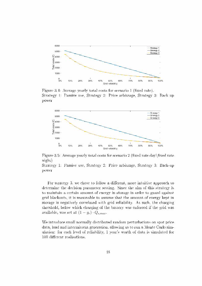
Figure 3.4: Average yearly total costs for scenario 1 (�xed rate).Strategy 1: Passive use, Strategy 2: Price arbitrage, Strategy 3: Back-uppower

Figure 3.5: Average yearly total costs for scenario 2 (�xed rate day\�xed ratenight)Strategy 1: Passive use, Strategy 2: Price arbitrage, Strategy 3: Back-uppower

For strategy 3, we chose to follow a di�erent, more intuitive approach todetermine the decision parameter setting. Since the aim of this strategy isto maintain a certain amount of energy in storage in order to guard againstgrid blackouts, it is reasonable to assume that the amount of energy kept instorage is negatively correlated with grid reliability. As such, the chargingthreshold, below which charging of the battery was enforced if the grid wasavailable, was set at (1− gr) ·Qs,max.

We introduce small normally distributed random perturbations on spot pricedata, load and intermittent generation, allowing us to run a Monte Carlo sim-ulation: for each level of reliability, 1 year's worth of data is simulated for100 di�erent realisations.

48

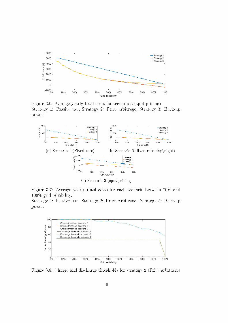
Figure 3.6: Average yearly total costs for scenario 3 (spot pricing)Strategy 1: Passive use, Strategy 2: Price arbitrage, Strategy 3: Back-uppower

(a) Scenario 1 (Fixed rate) (b) Scenario 2 (�xed rate day\night)

(c) Scenario 3 (spot pricing

Figure 3.7: Average yearly total costs for each scenario between 70% and100% grid reliability.Strategy 1: Passive use. Strategy 2: Price Arbitrage. Strategy 3: Back-uppower.

Figure 3.8: Charge and discharge thresholds for strategy 2 (Price arbitrage)

49

Most of the exogenous data are publicly available, this is the case for theresidential synthetic load curve [12], intermittent power production per kWp[13], and both �xed rate tari� structures[14], while electricity spot prices forthe Belgian market are made available after free registration on Belpex [8].

3.6 Results and limitations

In order to facilitate a clear discussion of the results, it is important to under-line the di�erence between scenarios and strategies, seeing as there are threeof each. Scenarios are tied to the rate structure for which the simulation wascarried out, while each of the strategies refers to a speci�c storage use strategyas outlined above. In addition, it is important to mention that the actualamount of total simulated costs does not have a high informational value, asthe exact value of total costs is in�uenced by the assumptions made earlier.However, the di�erence between cost patterns for the di�erent strategies andscenarios is informative, as any distortions due to made assumptions will bethe same across all reported results. As such, only pairwise comparisons ofour results will be presented.

For each scenario, the simulated resulting yearly operating costs for the en-tire range of grid reliability are presented in Fig. 3.4, 3.5 and 3.6, whileFig. 3.7 zooms in on the cost data for a more realistic range of grid reliabilityvalues for each of the three scenarios.

A �rst observation is that across all scenarios, the resultant cost behaviourfor strategies 2 and 3 is nearly identical up to 80% grid reliability. Thisobservation can be easily explained when looking at Fig. 3.8, which showsthe various charge/discharge thresholds for strategy 2 across all scenarios.Figure 3.8 merits a separate in-depth discussion, but when seen in the lightof the very similar cost behaviour of strategies 2 and 3 for low levels ofgrid reliability, it is su�cient to note that both strategies will exhibit sim-ilar charge/discharge behaviour: while the decision parameters are di�erent,both strategies will want to charge the battery whenever the grid is avail-able. Strategy 3 will do this because the battery storage will frequently becalled upon to provide power during one of the frequent blackouts, meaningthe state of charge of the battery will generally be low, leading to frequentcharging, while strategy 2 is driven to charging the battery whenever the gridis available because of the cost of shedding load as re�ected in the VOLL isseveral times higher than even the highest electricity price under spot pri-cing, meaning that it is bene�cial to charge the battery as much as possible,

50

even if this means the required energy needs to be bought from the grid.For the sake of clarity: this always buy behaviour is even true for strategy2 under scenario 1, even if price arbitrage is somewhat nonsensical under a�xed price regime. A notable exception to this buy at any cost behaviouris observed for strategy 2 under scenario 2: here the cost minimizing beha-viour is to charge the battery during periods when electricity is cheap -thisduring the o�-peak night-time period-, to discharge it during the day, exceptwhen grid reliability equals or exceeds 95%, as in these cases cost minimizingresults are achieved when any amount of stored electricity is immediatelyused. This means that the gains made discharging electricity from storagebefore losses from self-discharge are incurred outweigh the costs due to loadshedding during a grid outage, when no stored electricity is available.

Both strategies 2 and 3 show markedly lower costs than strategy 1 for theentire range of grid reliability. The gains to be made are large for low tomedium levels of grid reliability, and remain noticeable even up to 95% gridreliability, but the operating costs resultant from all strategies converge againfor a fully reliable grid. That being said, under a regime of spot-pricing forresidential consumers, price arbitrage is able to generate gains comparedto the other 2 strategies even at 100% grid reliability. Our results clearlyshow that even comparatively simple additions to passively using storage toaccommodate intermittent production surpluses are able to generate bene�ts.

As can be seen from Fig. 3.8, strategy 2 will engage in price arbitrage startingfrom a grid reliability level of 40%; the charge and discharge threshold curvesoverlap, meaning that for any grid price corresponding to a price percentilebelow the indicated curve, electricity will be stored, and for any price corres-ponding to a price percentile above the indicate curve, electricity will be usedfrom storage. It is interesting to note that for all scenarios, the charge anddischarge threshold coincide, meaning that the microgrid will always be anactive market participant, which means the impact of any kind of transactionfees could turn out to be signi�cant. This observation of a single thresholdalso means that strategy 2 can be simpli�ed somewhat, both during the pre-simulation parameter optimization as during the simulation itself, as havingseparate charge and discharge thresholds turns out to be super�uous. As gridreliability increases, strategy 2 becomes more risk taking, meaning electricitywill be sold sooner. This price arbitrage is perhaps most easily understoodas a form of peak shaving: since the spot price of electricity is driven by theaggregated load, or overall demand, periods of high price correspond to highoverall load.

51

True demand response, however, is not integrated into the model: storage isused to raise or lower the residual load that the electricity grid experiences,but at no point in time is the actual underlying load pro�le adapted. Thiscan lead to an overestimation of the actual costs, both for spot pricing re-gimes as for instances with less than 100% grid reliability. In both these casesa real household would probably be inclined to shift parts of their electricityconsumption to moments when it is cheaper or simply available.

3.7 Conclusion

In this paper we have presented an economical model of a microgrid, and dis-cussed the resulting cost function. We have touched upon the various driversof uncertainty impacting the cost minimisation of a microgrid and drawnup 3 possible strategies outlining the use of storage in a microgrid allowinga cost minimisation to be made. Performance of these three strategies hasbeen assessed on one simulated operating year of a residential Belgian mi-crogrid. Our results clearly show that even comparatively simple additionsto passively using storage to accommodate intermittent production surplusesare able to generate bene�ts.

52

Bibliography

[1] DOE, 2012. Summary report: 2012 DOE micrigrid workshop, Depart-ment of Energy.

[2] European Technology Platform, 2013. Smart Grids. On the WWW,December. url:http://www.smartgrids.eu.

[3] E. Handschin, F. Neise, H. Neumann, R. Schultz, 2006, "Optimal op-eration of dispersed generation under uncertainty using mathematicalprogramming". International Journal of Electrical Power & Energy Sys-tems, 28, November, pp 618-626.

[4] S. Mohammadi, B. Mozafari, S. Solimani, T. Niknal, 2013, "An Ad-aptive Modi�ed Fire�y Optimisation Algorithm based on Hong's PointEstimate Method to optimal operation management in a microgrid withconsideration of uncertainties". Energy, 51, pp 339-348.

[5] T. Niknam, F. Golestaneh, A. Malekpour, 2012, "Probabil-istic energy and operation management of a microgrid containingwind/photovoltaic/fuel cell generation and energy storage devices basedon point estimate method and self-adaptive gravitational search al-gorithm". Energy, 43, November, pp 427-437.

[6] A. Baziar, A. Kavousi-Fard, 2013, "Considering uncertainty in the op-timal energy management of renewable micro-grids including storagedevices". Renewable Energy, 59, pp 158-166.

[7] A.D. Hawkes, M.A. Leach, 2009, "Modelling high level system designand unit commitment for a microgrid". Applied Energy, 86, pp 1253-1265.

[8] Belpex, 2014. Market Data Services. On the WWW, November.url:https://www.belpex.be/services/market-data-services/.

53

[9] Elia, 2014. Facts & Figures 2013. On the WWW, November.url:http://www.elia.be/~/media/files/Elia/publications-2/facts-and-figures/Facts_Figures_EN_2013_LR.pdf.

[10] De redactie, 2014. Power Black-out Fears Re-emerge. On the WWW,August. url:http://deredactie.be/cm/vrtnieuws.english/News/1.2060840.

[11] De redactie, 2014. Power Shortages This Winter?. On theWWW, June. url:http://deredactie.be/cm/vrtnieuws.english/News/1.1995994.

[12] Synergrid, 2014. Synthetic Load Pro�les (SLP). On the WWW,October. url:http://www.synergrid.be/index.cfm?PageID=16896&language_code=NED.

[13] Elia, 2014. Solar-PV Power Generation Data. On the WWW,October. url:http://www.elia.be/en/grid-data/powergeneration/Solar-power-generation-data.

[14] Levver, 2014. Actuele kWh prijs elektriciteit in België.On the WWW, October. url:+http://www.levver.be/prijs-elektriciteit-per-kwh/ (in Dutch).

[15] D. Devogelaer, 2014, Belgische black-outs berekend: een kwnatit-atieve evaluatie van stroompannes in België. Federaal Planbureau.On the WWW, October. url:https://www.plan.be/admin/uploaded/201403170843050.WP_1403.pdf (in Dutch).

54

Chapter 4

Win-win possibilities through

capacity tari�s and battery

storage in microgrids1

Abstract

This paper investigates the impact of capacity tari� design on microgrids.While the possible bene�ts for utilities of capacity tari�s are well researched,comparatively little work has been done investigating the e�ects of capacitypricing on prosumers. Through simulating a grid connected microgrid andsolving the day-ahead dispatch problem for a calendar year, we show that awell-designed capacity tari� will not only smooth out demand pro�les, butcould also lead to less erratic charge/discharge cycles in a real-time pricingscenario, lessening battery degradation. These results show that a properlydesigned capacity tari� has the potential to be bene�cial for both the utilitiesas well as the battery-owning prosumer. Furthermore, we propose a new,heuristic approach to solve the day-ahead economic dispatch problem, whichwe prove to be e�ective and e�cient. Additionally, we demonstrate that ournovel approach does not impose mathematical restrictions such as continuousdi�erentiability of the objective function.

1This chapter has been submitted for publication to Applied Energy as Milis, K.,

Peremans H., Springael J., Van Passel S. Win-win possibilities through capacity tari�s and

battery storage in microgrids

55

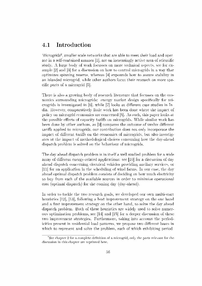
4.1 Introduction

Microgrids2, smaller scale networks that are able to meet their load and oper-ate in a self-contained manner [1], are an increasingly active area of scienti�cstudy. A large body of work focusses on more technical aspects, see for ex-ample [2] and [3] for a discussion on how to control microgrids in a way thatoptimizes spinning reserve, whereas [4] expounds how to assure stability inan islanded microgrid, while other authors focus their research on more spe-ci�c parts of a microgrid [5].

There is also a growing body of research literature that focusses on the eco-nomics surrounding microgrids: energy market design speci�cally for mi-crogrids is investigated in [6], while [7] looks at di�erent case studies in In-dia. However, comparatively little work has been done where the impact ofpolicy on microgrid economics are concerned [8]. As such, this paper looks atthe possible e�ects of capacity tari�s on microgrids. While similar work hasbeen done by other authors, as [9] compares the outcome of twelve di�erenttari�s applied to microgrids, our contribution does not only incorporate theimpact of di�erent tari�s on the economics of microgrids, but also investig-ates at the impact of methodological choices concerning how the day-aheaddispatch problem is solved on the behaviour of microgrids.

The day ahead dispatch problem is in itself a well studied problem for a widearray of di�erent energy-related applications: see [10] for a discussion of dayahead dispatch concerning electrical vehicles providing ancilary services, or[11] for an application in the scheduling of wind farms. In our case, the dayahead optimal dispatch problem consists of deciding on how much electricityto buy from each of the available sources in order to minimize operationalcost (optimal dispatch) for the coming day (day-ahead).

In order to tackle the two research goals, we developed our own multi-startheuristics [12], [13], following a best improvement strategy on the one handand a �rst improvement strategy on the other hand, to solve the day aheaddispatch problem. Both of these heuristics are widely used to solve numer-ous optimization problems, see [14] and [15] for a deeper discussion of thesetwo improvement strategies. Furthermore, taking into account the period-icities present in residential load patterns, we propose two di�erent bases inwhich to represent and solve the problem, each of which exhibiting period-

2See chapter 2 for a complete de�nition of a microgrid, only the parts relevant for the

discussion in this chapter are reprinted here.

56

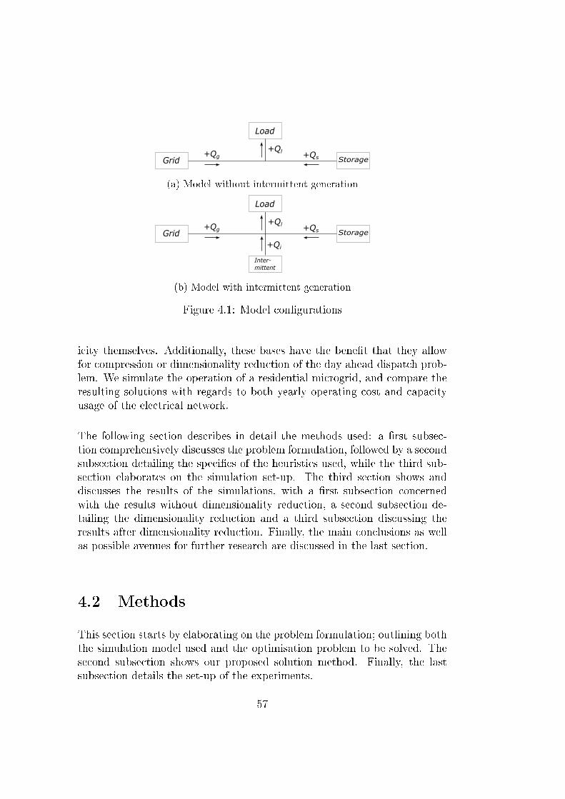
Grid

Load

Storage+Qg +Qs

+Ql

(a) Model without intermittent generation

Grid

Load

Storage+Qg +Qs

+Ql

Inter-mittent

+Qi

(b) Model with intermittent generation

Figure 4.1: Model con�gurations

icity themselves. Additionally, these bases have the bene�t that they allowfor compression or dimensionality reduction of the day ahead dispatch prob-lem. We simulate the operation of a residential microgrid, and compare theresulting solutions with regards to both yearly operating cost and capacityusage of the electrical network.

The following section describes in detail the methods used: a �rst subsec-tion comprehensively discusses the problem formulation, followed by a secondsubsection detailing the speci�cs of the heuristics used, while the third sub-section elaborates on the simulation set-up. The third section shows anddiscusses the results of the simulations, with a �rst subsection concernedwith the results without dimensionality reduction, a second subsection de-tailing the dimensionality reduction and a third subsection discussing theresults after dimensionality reduction. Finally, the main conclusions as wellas possible avenues for further research are discussed in the last section.

4.2 Methods

This section starts by elaborating on the problem formulation; outlining boththe simulation model used and the optimisation problem to be solved. Thesecond subsection shows our proposed solution method. Finally, the lastsubsection details the set-up of the experiments.

57

4.2.1 Problem formulation

Consider the economic dispatch problem for a macrogrid connected microgrid.Our model, as shown in �g 4.1 encompasses exogenous load, battery storage,and possibly exogenously driven local intermittent generation. Speci�cally,we determine the amount of electricity sold or bought from the macrogridthat will minimise operating costs over a rolling window with a variable hori-zon H. The optimisation problem is solved for the �rst horizon-length set ofhours of the year, after which the obtained solution for the �rst hour is saved.Then, the optimisation problem is solved for the next horizon window, butnow starting with hour two of the year, as opposed to hour one. Again, thesolution for the �rst hour, i.e. hour two of the year, is kept. This process isrepeated until a solution has been found for the entire year.

The operating cost, to be minimised, has two components: an energy com-ponent, and a capacity component. The energy component is the productof a) the amount of energy withdrawn from or injected into the grid overone hour, Qg(t), and b) the price for energy during that hour, Pg(t). Thisprice can either be determined by �xed pricing, time of use pricing, or realtime market pricing. The capacity component of the cost function re�ectsa capacity block pricing scheme, based on the work of Schreiber et al. [19]where all capacity used up to a certain level Cbar will be paid at a rate Cp1and all capacity used above this level is charged at the higher rate Cp2. Wechoose to use this speci�c design since Schreiber et al. reported the bestresults with this kind of capacity market design in [19].

While the energy costs might be negative, re�ecting a net bene�t for the mi-crogrid as it sells excess electricity to the macrogrid, the capacity componentof the cost function will always be positive. This is by design, since injectingelectricity into the macrogrid uses the same infrastructure as withdrawingenergy from the grid. Due to the granularity of one hour and our assumptionthat the electric power withdrawn from, or injected to the grid is uniformwithin each hour, Qg represents both the amount of energy, in kWh, as wellas the peak load, in kW.

First, the simple case of a model with a battery without self-discharge isdiscussed. Then, this model is extended by integrating self-discharge of thebattery component in the model. The �nal subsection describes the imple-mented model in which we transform the problem, so far formulated in thetime domain, into a new problem by choosing an appropriate set of basisfunctions.

58

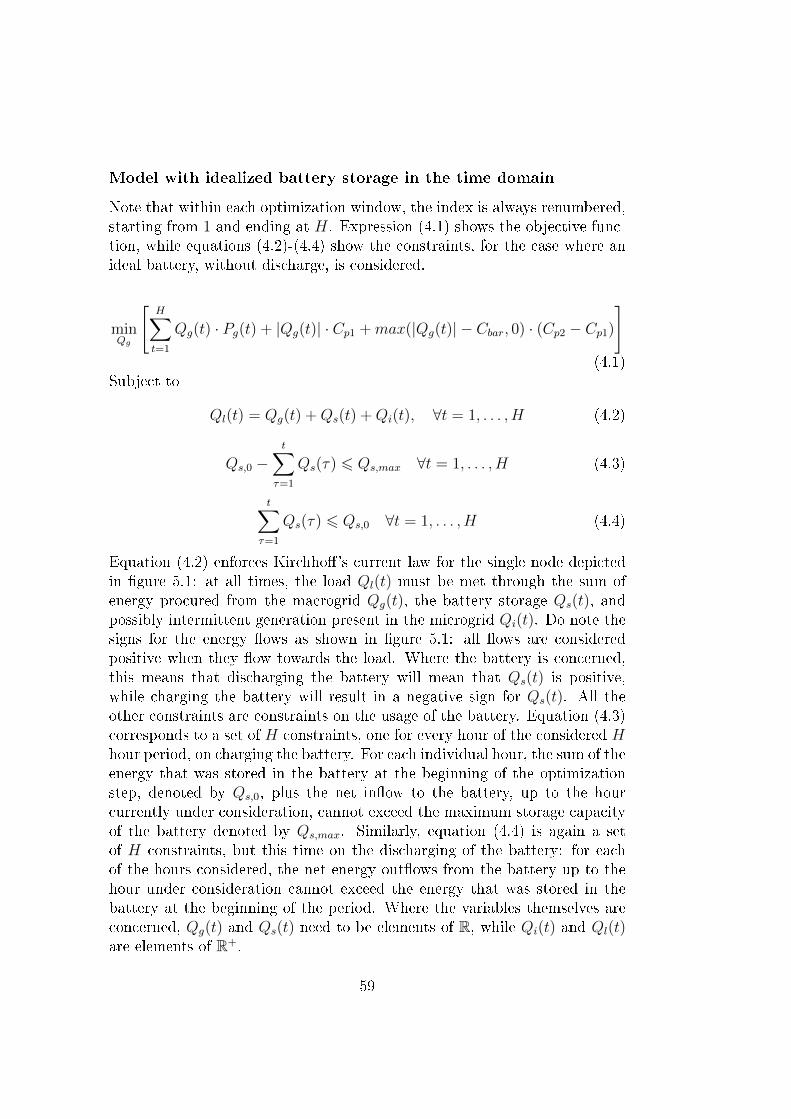
Model with idealized battery storage in the time domain

Note that within each optimization window, the index is always renumbered,starting from 1 and ending at H. Expression (4.1) shows the objective func-tion, while equations (4.2)-(4.4) show the constraints, for the case where anideal battery, without discharge, is considered.

minQg

[H∑t=1

Qg(t) · Pg(t) + |Qg(t)| · Cp1 +max(|Qg(t)| − Cbar, 0) · (Cp2 − Cp1)

](4.1)

Subject to

Ql(t) = Qg(t) +Qs(t) +Qi(t), ∀t = 1, . . . , H (4.2)

Qs,0 −t∑

τ=1

Qs(τ) 6 Qs,max ∀t = 1, . . . , H (4.3)

t∑τ=1

Qs(τ) 6 Qs,0 ∀t = 1, . . . , H (4.4)

Equation (4.2) enforces Kirchho�'s current law for the single node depictedin �gure 5.1: at all times, the load Ql(t) must be met through the sum ofenergy procured from the macrogrid Qg(t), the battery storage Qs(t), andpossibly intermittent generation present in the microgrid Qi(t). Do note thesigns for the energy �ows as shown in �gure 5.1: all �ows are consideredpositive when they �ow towards the load. Where the battery is concerned,this means that discharging the battery will mean that Qs(t) is positive,while charging the battery will result in a negative sign for Qs(t). All theother constraints are constraints on the usage of the battery. Equation (4.3)corresponds to a set of H constraints, one for every hour of the considered Hhour period, on charging the battery. For each individual hour, the sum of theenergy that was stored in the battery at the beginning of the optimizationstep, denoted by Qs,0, plus the net in�ow to the battery, up to the hourcurrently under consideration, cannot exceed the maximum storage capacityof the battery denoted by Qs,max. Similarly, equation (4.4) is again a setof H constraints, but this time on the discharging of the battery: for eachof the hours considered, the net energy out�ows from the battery up to thehour under consideration cannot exceed the energy that was stored in thebattery at the beginning of the period. Where the variables themselves areconcerned, Qg(t) and Qs(t) need to be elements of R, while Qi(t) and Ql(t)are elements of R+.

59

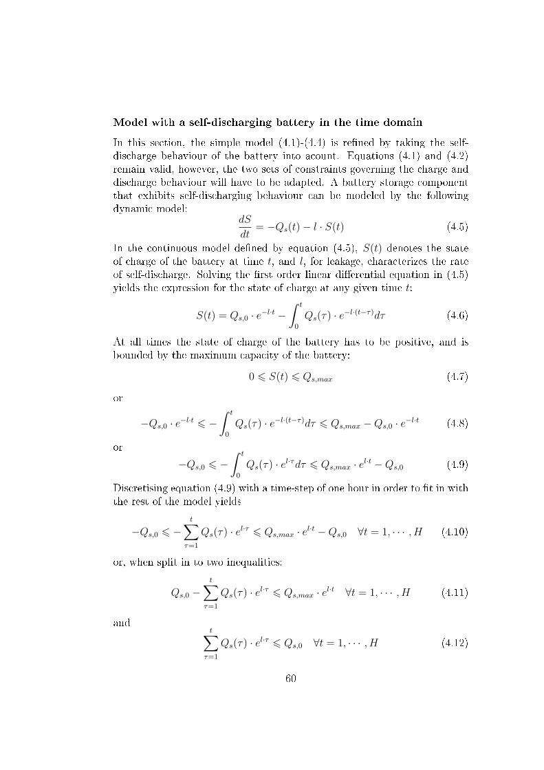
Model with a self-discharging battery in the time domain

In this section, the simple model (4.1)-(4.4) is re�ned by taking the self-discharge behaviour of the battery into acount. Equations (4.1) and (4.2)remain valid, however, the two sets of constraints governing the charge anddischarge behaviour will have to be adapted. A battery storage componentthat exhibits self-discharging behaviour can be modeled by the followingdynamic model:

dS

dt= −Qs(t)− l · S(t) (4.5)

In the continuous model de�ned by equation (4.5), S(t) denotes the stateof charge of the battery at time t, and l, for leakage, characterizes the rateof self-discharge. Solving the �rst order linear di�erential equation in (4.5)yields the expression for the state of charge at any given time t:

S(t) = Qs,0 · e−l·t −∫ t

0

Qs(τ) · e−l·(t−τ)dτ (4.6)

At all times the state of charge of the battery has to be positive, and isbounded by the maximum capacity of the battery:

0 6 S(t) 6 Qs,max (4.7)

or

−Qs,0 · e−l·t 6 −∫ t

0

Qs(τ) · e−l·(t−τ)dτ 6 Qs,max −Qs,0 · e−l·t (4.8)

or

−Qs,0 6 −∫ t

0

Qs(τ) · el·τdτ 6 Qs,max · el·t −Qs,0 (4.9)

Discretising equation (4.9) with a time-step of one hour in order to �t in withthe rest of the model yields

−Qs,0 6 −t∑

τ=1

Qs(τ) · el·τ 6 Qs,max · el·t −Qs,0 ∀t = 1, · · · , H (4.10)

or, when split in to two inequalities:

Qs,0 −t∑

τ=1

Qs(τ) · el·τ 6 Qs,max · el·t ∀t = 1, · · · , H (4.11)

andt∑

τ=1

Qs(τ) · el·τ 6 Qs,0 ∀t = 1, · · · , H (4.12)

60

Equations (4.11) and (4.12) each represent H constraints, one for each of thehours comprised in the time window under consideration, on the chargingand discharging of the battery respectively.

Model as expressed in terms of a general H-dimensional set of basis

functions

The models build in the previous two sections are all written with the as-sumption that the problem is being worked on in the time domain. The setof H setpoints that are generated for the grid and the battery can also beseen as a single vector:

Q̄s = [Qs(1), · · · , Qs(H)] (4.13)

Q̄g = [Qg(1), · · · , Qg(H)] (4.14)

It is possible to reformulate the problem to make use of any H dimensionalbase consisting of basis vectors b̄h and coe�cients sh and gh , such that:

Q̄s =H∑h=1

sh · b̄h (4.15)

Q̄g =H∑h=1

gh · b̄h (4.16)

Substituting equations (4.15) and (4.16) into equations (4.11) and (4.12)yields:

Qs,0 −t∑

τ=1

H∑h=1

sh · b̄h(τ) · el·τ 6 Qs,max · el·t ∀t = 1, · · · , H (4.17)

t∑τ=1

H∑h=1

sh · b̄h(τ) · el·τ 6 Qs,0 ∀t = 1, · · · , H (4.18)

Equations (4.17) and (4.18) are the formulations of the constraints on thecharging and discharging of the battery used in the �nal model. Rewritingthe objective function and the �rst constraint leads to the �nal formulationof the optimisation problem that will be solved:

mingh

[H∑h=1

gh · b̄h · P̄g + |H∑h=1

gh · b̄h| · C̄p1 +max(|H∑h=1

gh · b̄h| − C̄bar, 0) · (C̄p2 − C̄p1)

](4.19)

61

Subject to

Q̄l =H∑h=1

gh · b̄h +H∑h=1

sh · b̄h + Q̄i (4.20)

Qs,0 −t∑

τ=1

H∑h=1

sh · b̄h(τ) · el·τ 6 Qs,max · el·t ∀t = 1, · · · , H (4.21)

t∑τ=1

H∑h=1

sh · b̄h(τ) · el·τ 6 Qs,0∀t = 1, · · · , H (4.22)

In equations (4.21) and (4.22), b̄h(τ) denotes the τ − th element of the h− thbasis vector. Additionally, all of the assumed exogenous variables in themodel have been rewritten as vectors for consistency. P̄g, Q̄l and Q̄i eachcontain H values of the corresponding dataset for each of the H hours of theconsidered time period, while C̄p1, C̄p2 and C̄bar are all size H vectors, withall elements being equal to Cp1, Cp2 and Cbar respectively. All the productsin equation (4.19) between vectors are scalar products.

4.2.2 Heuristic solution method

It is our goal to investigate whether it is possible to solve the economic dis-patch problem for a microgrid, as outlined by equations (4.19) to (4.22), witha subset of basis vectors. Ideally, this compression should allow for shorterrun times of the algorithm, depending on which components are kept anddiscarded during the compression step. However, the compression shouldalso maintain a similar economic performance in terms of cost, in compar-ison with the same algorithm without compression. In order to get insight,we implemented a heuristic solver, in such a manner that we would havefull control over the algorithm. We solved the economic dispatch problem inthree di�erent bases to test the hypothesis with regard to the choice of basisimpacting the quality of the compression.

The following subsections elaborate on our solution method: a �rst sub-section shows the implemented heuristic. The next subsection details thedi�erent bases, used to solve the problem, while a �nal subsection outlinesthe set-up of the di�erent simulations.

Heuristic search

We implemented two di�erent, multi-start heuristics to solve the problemoutlined above using a best improvement and �rst improvement strategy.

62

Start

Until stopping condition is met

Yes

No

No

Yes

At least 1cheaper &feasible solution?

Generate startingsolution

Generate candidatesolutions

Save cheapestsolution

Cheapest solutionbecomes startingsolution

Generate randomsolution

Randomsolutionfeasible?

Save cheapestsolution

Cheapest solutionbecomes startingsolution

(a) Best improvement

Start

Until stopping condition is met

Yes

No

No

Yes

At least 1cheaper &feasible solution?

Generate startingsolution

Generate candidatesolutions

Save first cheapersolution

Cheapest solutionbecomes startingsolution

Generate randomsolution

Randomsolutionfeasible?

Save cheapestsolution

Cheapest solutionbecomes startingsolution

(b) First improvement

Figure 4.2: Heuristic �owcharts

63

Both strategies are depicted schematically in �gs. 4.2a and 4.2b respectively.Best improvement, on the one hand, evaluates h pairs of candidate solutionsper optimisation step consisting of a positive and a negative step in each ofthe basis directions. If none of the evaluated solutions have a lower cost thanthe previous solution -or start solution, for the �rst iteration-, a random feas-ible solution is generated. The corresponding cost is calculated and the newsolution is used as starting point for the next iteration. If there is at leastone of the candidate solutions feasible with a lower cost, the feasible solutionwith the lowest cost will be selected. First improvement, on the other hand,will generate the same set of h candidate solution pairs, and will also check ifat least one of the generated candidate solutions is feasible with a lower cost,but will not select the feasible solution with the lowest cost, but rather the�rst feasible solution encountered with a cost lower than the cost of the solu-tion found in the previous iteration. �First� is in this case de�ned by the orderof the coe�cients gh: if δ is the stepsize and Q̄g,pre is the solution obtainedat the end of the previous optimization step, then Q̄g,pre + δ · g1 · b̄1 is said tobe the �rst candidate solution followed by Q̄g,pre− δ · g1 · b̄1, Q̄g,pre + δ · g2 · b̄2the third and so on.

Both of the implemented heuristics run through the optimization steps un-til one of two stopping criteria is met: the heuristic will stop after either ade�ned maximum number of iterations have been reached, or when the dif-ference between the best solution found untill now and the current solutionis smaller than a certain threshold precision.

Bases3

This research investigates whether or not exploiting the structure presentin the problem impacts the the operation of the algorithm used, leading toeither cheaper solutions, or similar solutions found with less computationaltime elapsed. A natural candidate basis to investigate this is the sequentiallyordered Walsh matrix of order h. Each of the columns of the matrix is takenas one of the h basis vectors, as each column has an increasing amount ofsign switches as can be seen in �gure 4.3a, which in our model, correspondsto a higher frequency of switching between charge and discharge. This meansthat some of the patterns that one would expect to �nd in the solution arealready present in the base matrix, such as the �rst basis vector providing forthe constantly present base load, while the second basis term is well suited

3Please refer to Appendix A for a more in-depth discussion of the underlying math-

ematical concepts

64

to model usage patterns with a periodicity of 8 hours, such as a working day.

However, Walsh matrices only exists for orders equal to powers of 2, meaningthat there is no Walsh matrix of order 24, which is the usual time horizonconsidered for economic dispatch problems. As the time horizon for whichwe solve our optimization problem is �exible, this is not inherently a prob-lem: the basis formed by the Walsh matrix of order 16 can be used to solvethe optimization problem, and is therefore one of the bases used in this paper.

Additionally, if we are willing to forgo the increasing amount of sign changesper column, the Hadamard matrix is similar to the Walsh matrix: comparefor instance �gure4.3a with �gure 4.3b and note that the Walsh matrix con-tains a large range of sign changes per column, whereas the correspondingHadamard matrix does not. In order to construct a Hadamard matrix, it isonly required that order of the matrix to is even, meaning that a Hadamardmatrix of order 24 can be used as a basis to solve the economic dispatchproblem for a twenty-four hour time horizon.

As is clear from the comparison between �gures 4.3a, 4.3b and 4.3c, while thepattern of increasing sign changes is still somewhat present in the Hadamardmatrix of order 16, it is almost completely gone from the Hadamard matrixof order 24. We use both Hadamard matrices as a basis as the comparisonbetween the results of the Walsh and Hadamard matrix of order 16 will grantinsight as to whether the sequential ordering is important, and comparingbetween the results obtained with the Hadamard matrix of order 16 and theHadamard matrix of order 24 allows for the investigation of the impact ofthe chosen horizon on the outcome of the optimization.

Finally, for each of the considered time horizons, the standard basis, basedon the identity matrix of the corresponding order (see �gs. 4.3d and 4.3e) ofthat dimension was also used, to provide a baseline against which perform-ance of the other bases could be compared to, both in terms of number ofiterations as in terms of total operating costs.

Each of the bases was also re-scaled to ensure that each charge-dischargecycle does not violate the capacity constraints of the battery. When a randomsolution is generated, as part of the multi-start heuristic, a linear combinationof basis vectors with a norm not exceeding 1 is used. While this approachdoes not guarantee feasible solutions, as the feasibility is contingent upon theamount of energy stored in the battery at the beginning of the time periodt currently being optimized, it does ensure that no solutions are generated

65

2 4 6 8 10 12 14 16

2

4

6

8

10

12

14

16

(a) Walsh matrix of order 16

2 4 6 8 10 12 14 16

2

4

6

8

10

12

14

16

(b) Hadamard matrix of order 16

5 10 15 20

5

10

15

20

(c) Hadamard matrix of order 24

2 4 6 8 10 12 14 16

2

4

6

8

10

12

14

16

(d) Identity matrix of order 16

5 10 15 20

5

10

15

20

(e) Identity matrix of order 24

Figure 4.3: Overview of the di�erent bases. Yellow cells always correspondto a value of one, blue cells to a value of minus one in sub�gures a throughc, and zero in sub�gures d and e.

66

that are by construction infeasible.

4.2.3 Simulation set-up

We solve the optimization problem outlined in eqs(4.19) to (4.22) for a me-dian Belgian household with an annual electricity demand of 3600 kWh. Thestorage component is modeled after Tesla Powerwall and sized at a maximumcapacity of 7 kWh. In the literature, self discharge rates for Li-Ion batter-ies are reported between 5% and 10%, but these are always reported for atwenty-four hour period at minimum. To arrive at a 10% discharge after 24hours, the discharge in our simulation was modeled at a �at rate of 0.4%per hour. The block capacity tari� design is based upon the design thatproduced the best results in [19], with Cbar set at 75% of the annual loadpeak, Cp1 at 0.0584 e/kW and Cp2 at 0.1872 e/kW . This block capacitydesign is compared to a �xed capacity tari� of 0.0652 e/kW , and a casewithout a capacity tari�; see �gure 4.4 for a visual representation of a blockcapacity tari�. In the simulations where intermittent generation is part ofthe simulated microgrid, this was modeled as 2.1 kWp of PV generation, torepresent a modal Belgian household with PV generation. Where the heur-istics themselves are concerned, the stopping criteria used are maximum 1000optimization iterations per time window and a precision of 0.01 e.

Both cases with and without a capacity tari� are simulated for system con�g-urations with and without the inclusion of solar PV, resulting in four di�erentset-ups. Each of these set-ups is then solved with each of the �ve di�erentbases outlined above. The four di�erent set-ups are also solved using baseswith reduced dimensionality, based on the Walsh basis and the two Hadam-ard bases. Each of the mentioned simulations is executed for �ve di�erentrealisations of the same year, providing insight into the robustness and sta-bility of the obtained results.

The exogenous datasets used in the simulations, are all sourced from vari-ous Belgian electricity market actors: the consumer load is based on thesynthetic load curves provided by Synergrid [16], the belgian federation ofelectricity- and natural gasgrid operators, while the electricity price pro�leused was obtained form EPEX SPOT Belgium [17], the Belgian power ex-change operator. The intermittent generation in the simulation is providedby solar PV, for which hourly generation data for Belgium is provided by theBelgian TSO, Elia [18].

67

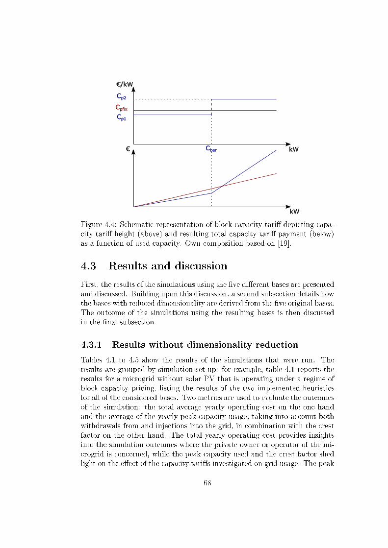
Cpfix

Cp2

Cp1

€/kW

kW

kW

€ Cbar

Figure 4.4: Schematic representation of block capacity tari� depicting capa-city tari� height (above) and resulting total capacity tari� payment (below)as a function of used capacity. Own composition based on [19].

4.3 Results and discussion

First, the results of the simulations using the �ve di�erent bases are presentedand discussed. Building upon this discussion, a second subsection details howthe bases with reduced dimensionality are derived from the �ve original bases.The outcome of the simulations using the resulting bases is then discussedin the �nal subsection.

4.3.1 Results without dimensionality reduction

Tables 4.1 to 4.5 show the results of the simulations that were run. Theresults are grouped by simulation set-up: for example, table 4.1 reports theresults for a microgrid without solar PV that is operating under a regime ofblock capacity pricing, listing the results of the two implemented heuristicsfor all of the considered bases. Two metrics are used to evaluate the outcomesof the simulation: the total average yearly operating cost on the one handand the average of the yearly peak capacity usage, taking into account bothwithdrawals from and injections into the grid, in combination with the crestfactor on the other hand. The total yearly operating cost provides insightsinto the simulation outcomes where the private owner or operator of the mi-crogrid is concerned, while the peak capacity used and the crest factor shedlight on the e�ect of the capacity tari�s investigated on grid usage. The peak

68

capacity usage and the crest factor provide similar, but distinct information:the peak capacity usage is straightforward, and shows peak usage of the elec-trical network by the microgrid, while the crest factor is de�ned as the ratioof the peak capacity usage and the RMS value of the capacity usage overthe year. As such, it is a measure of �peakiness� in the capacity usage, as itprovides information on the ratio of the highest capaty peak to the averagecapacity used. In terms of the grid, it also correlates with the utilisation ofassets that make up the distribution grid. In each table, the best results forall considered metrics are printed in boldface for each of the used heuristics.

A few general trends are immediately apparent when it comes to averageyearly operating cost: the best improvement strategy outperforms the �rstimprovement strategy in all but two cases. Furthermore, in these two cases,the results of both improvement strategies are less then one standard de-viation apart. A second general observation is that the results across allsimulations are quite stable, as evidenced by the small standard deviations.Another trend evident across all runs is that the solutions obtained for abases with dimensionality 16 consistently outperform the problem formula-tions with dimensionality 24 of the same problem, except in the two �xedcapacity pricing scenarios. In the case of �xed capacity pricing without solarPV, the results of the three non-standard bases are very close together, asshow in table 4.3. The overall better performance of dimensionality 16 basesseems to indicate that from a computational point of view it is better tosolve a larger number of smaller problems, as opposed to a smaller numberof larger problems. However, when comparing the average yearly peak usageacross all simulations ran, it is clear that the simulations with a twenty-fourhour decision horizon have on the whole lower capacity usage peaks than thecorresponding simulations with a sixteen hour decision horizon, the reasonbeing that the base twenty-four representations have more hours to smoothout any demand or supply peak.

Furthermore, only in one of the twelve investigated cases is the best perform-ing algorithm one that is using the standard basis, as table 4.2 shows that theheuristic using the standard 16 base obtains the lowest cost in a system withsolar PV, operating under block capacity pricing. Across all di�erent systemset-ups and heuristics, the Hadamard 16 base is the best performing of dif-ferent bases tried, reporting the lowest average operating costs in six out oftwelve cases, while the Walsh 16 base obtains the lowest average costs in threeout of twelve cases. On the one hand, this means that one of our researchhypotheses, that the increase of frequency present in Walsh basis is a prop-erty which would allow the heuristic to �nd better solutions more quickly, is

69

not upheld. On the other hand, these results do show that another researchhypothesis is upheld: the non-standard bases outperform the standard bases.

On the whole, the relationship between the average yearly operating costsand the capacity peaks seems somewhat counter-intuitive at �rst, as lowerpeak usage of the grid doesn't really coincide with lower total operatingcosts when comparing results for the same scenario set-up: the �rst improve-ment strategy regularly reports lower capacity usage peaks but is consistentlyout-performed by the best improvement strategy where total costs are con-cerned. It should be noted, however, that varying the weights of the energycomponent and the capacity component in the objective function, such as byincreasing Cp1 or Cp2 is out of scope for this study, but these results seem toindicate that the relative merits of using �rst improvement or best improve-ment might be contingent on these relative weights.

Table 4.5 deserves special attention, as at �rst glance the results reportedtherein for the best improvement strategy in both the Hadamard bases aswell as the Walsh basis seem almost erroneous. However, when the pattern ofelectricity bought from and sold to the grid is examined, it is clear that thesesolutions engage in almost perfect price arbitrage, by buying up and storinggrid electricity when the price is low in order to sell this electricity back tothe grid when the price is high. Consequently, the grid is heavily used inthis case, as doing so is free, meaning that the only price signal the systemresponds to, is the electricity price. Comparing these results to the resultsobtained with block or �xed capacity pricing also immediately proves therole that capacity tari� can play in stabilizing the grid, by limiting excessivebuying and selling of electricity solely to exploit arbitrage opportunities: ca-pacity tari�s act as transaction costs, rendering hour to hour arbitrage basedon minor price di�erences no longer pro�table.

In a similar vein, the usefulness of capacity pricing is also demonstrated bycomparing the results with and without the addition of solar PV for the threedi�erent capacity payment schemes, as they clearly show that di�erent kindsof capacity tari� lead to the electricity generated by the PV panels being usedin a di�erent way. As can be expected, tables 4.5 & 4.6 show that in the casewhere there is no capacity tari�, most of the electricity generated by the solarpanels is sold to the grid, driving down the average yearly operating cost,while signi�cantly heightening the capacity usage peak. Conversely, tables4.1 & 4.2 show that under a system of block capacity pricing, the addition ofsolar PV has a much more nuanced impact on the behaviour of the system,slightly increasing or decreasing the peak capacity usage, depending on the

70

heuristic used. As evidenced by tables 4.3 & 4.4 a �xed capacity tari� leadsto an outcome in between these two extremes.

Furthermore, table 4.5 also shows the e�ectiveness of solving the economicdispatch problem using one of the proposed non-standard bases: the al-gorithm using these representations is able to �nd and exploit these arbitrageopportunities within the limited number of iterations available, whereas thesame algorithm solving the same problem using a standard problem repres-entation is not.

When comparing the average yearly operating cost between the three di�er-ent capacity tari� schemes, �xed capacity pricing and block capacity pricingare quite close together, while a system with no capacity tari�s predictablyresults in much lower operating costs. However, this favourable individualoutcome is o�set by heavy use of the electrical grid. While the study of thisresulting externality is outside the scope of this study, this is clearly an un-favourable outcome for society. The choice between �xed capacity pricing orblock capacity pricing is more interesting: consumers without solar PV areslightly better o� under a block capacity scheme than under �xed capacitypricing, while the reverse is true for consumers with solar PV. As can be seenfrom �gure 4.4, block capacity pricing is cheaper than �xed capacity pricingas long as the capacity barrier is not heavily exceeded. It is only for capacityusage consistently exceeding the capacity barrier that �xed capacity pricingbecomes cheaper for the consumer than block capacity pricing. Applied tothe reported results, this means that under block capacity pricing, the al-gorithms stay close to enough or below the capacity barrier so that the totalyearly operating costs is lower than in the case with a �xed capacity tari�.The addition of solar PV to the system, however, means that there is anexcess of energy to be sold to the grid, driving up capacity usage, resultingin more capacity payments under a block tari� scheme than under a �xedcapacity payment scheme.

The crest factors mimic the behaviour of the peak capacity usage, in that alow peak capacity usage will generally also correspond to a low crest factor.Furthermore, just as with peak capacity usage, the �rst improvement strategyresults in lower crest factors than the best improvement strategy for the samescenario set-up. When comparing the scenarios with and without solar PV,how the crest factor changes depends on the basis used for both block ca-pacity pricing and �xed capacity pricing: adding solar PV drives the crestfactor down for the heuristics using the standard bases, and increases thecrest factor for the non-standard bases.

71

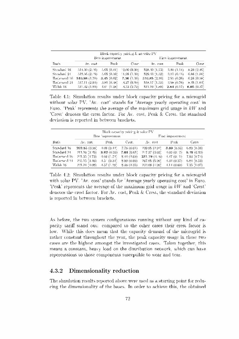
Block capacity pricing & no solar PVBest improvement First improvement

Basis Av. cost Peak Crest Av. cost Peak Crest

Standard 16 514.30 (2.46) 5.65 (0.41) 12.00 (0.90) 528.40 (1.73) 3.80 (1.14) 8.20 (2.46)Standard 24 518.56 (2.49) 5.65 (0.59) 11.98 (1.30) 529.43 (1.52) 3.17 (0.45) 6.86 (1.00)Hadamard 16 510.98 (1.70) 3.45 (0.62) 7.36 (1.36) 510.85 (2.16) 2.95 (0.26) 6.26 (0.58)Hadamard 24 517.11 (2.04) 3.88 (0.38) 8.27 (0.80) 518.17 (1.55) 3.98 (0.76) 8.45 (1.64)Walsh 16 511.32 (1.88) 4.01 (1.28) 8.53 (2.72) 511.19 (1.88) 2.84 (0.17) 6.05 (0.37)

Table 4.1: Simulation results under block capacity pricing for a microgridwithout solar PV. 'Av. cost' stands for 'Average yearly operating cost' inEuro. 'Peak' represents the average of the maximum grid usage in kW and'Crest' denotes the crest factor. For Av. cost, Peak & Crest, the standarddeviation is reported in between brackets.

Block capacity pricing & solar PVBest improvement First improvement

Basis Av. cost Peak Crest Av. cost Peak Crest

Standard 16 202.85 (3.98) 4.09 (0.42) 7.78 (0.61) 239.95 (2.92) 3.89 (0.35) 6.80 (0.59)Standard 24 211.16 (3.25) 3.82 (0.33) 7.03 (0.61) 247.37 (3.03) 4.03 (0.47) 6.49 (0.83)Hadamard 16 221.35 (4.73) 4.60 (1.72) 8.44 (2.69) 231.19 (4.46) 4.47 (0.41) 7.93 (0.74)Hadamard 24 225.15 (3.46) 4.54 (0.34) 8.09 (0.60) 267.05 (5.99) 4.32 (0.37) 6.84 (0.53)Walsh 16 221.24 (4.08) 4.57 (1.29) 8.38 (2.35) 232.09 (4.99) 4.14 (0.60) 7.35 (1.07)

Table 4.2: Simulation results under block capacity pricing for a microgridwith solar PV. 'Av. cost' stands for 'Average yearly operating cost' in Euro.'Peak' represents the average of the maximum grid usage in kW and 'Crest'denotes the crest factor. For Av. cost, Peak & Crest, the standard deviationis reported in between brackets.

As before, the two system con�gurations running without any kind of ca-pacity tari� stand out: compared to the other cases their crest factor islow. While this does mean that the capacity demand of the microgrid israther constant throughout the year, the peak capacity usage in these twocases are the highest amongst the investigated cases. Taken together, thismeans a constant, heavy load on the distribution network, which can haverepercussions to those components susceptible to wear and tear.

4.3.2 Dimensionality reduction

The simulation results reported above were used as a starting point for redu-cing the dimensionality of the bases. In order to achieve this, the obtained

72

Fixed capacity pricing & no solar PVBest improvement First improvement

Basis Av. cost Peak Crest Av. cost Peak Crest

Standard 16 523.21 (0.52) 6.53 (0.22) 12.33 (0.41) 544.94 (0.53) 3.78 (0.53) 7.61 (1.05)Standard 24 528.16 (0.48) 6.06 (0.40) 11.57 (0.78) 548.10 (0.53) 3.74 (0.45) 7.48 (0.89)Hadamard 16 520.62 (0.69) 5.54 (0.57) 9.80 (1.03) 519.67 (0.75) 5.14 (0.65) 9.20 (1.17)Hadamard 24 519.11 (0.56) 5.54 (0.46) 8.99 (0.72) 525.77 (0.68) 6.06 (0.74) 10.44 (1.22)Walsh 16 520.53 (0.61) 5.09 (0.60) 8.98 (1.04) 520.76 (0.63) 5.26 (1.02) 9.42 (1.84)

Table 4.3: Simulation results under �xed capacity pricing for a microgridwithout solar PV. 'Av. cost' stands for 'Average yearly operating cost' inEuro. 'Peak' represents the average of the maximum grid usage in kW and'Crest' denotes the crest factor. For Av. cost, Peak & Crest, the standarddeviation is reported in between brackets.

Fixed capacity pricing & solar PVBest improvement First improvement

Basis Av. cost Peak Crest Av. cost Peak Crest

Standard 16 187.04 (0.95) 6.07 (0.54) 8.91 (0.83) 238.34 (0.86) 6.45 (0.32) 8.21 (0.37)Standard 24 201.82 (1.66) 6.39 (0.29) 9.19 (0.44) 248.27 (1.56) 6.62 (0.59) 8.38 (0.75)Hadamard 16 186.76 (0.89) 6.32 (0.69) 9.29 (0.99) 192.53 (0.81) 6.03 (0.56) 8.98 (0.85)Hadamard 24 181.72 (1.30) 5.93 (0.66) 8.54 (0.93) 204.38 (0.56) 5.62 (0.54) 7.75 (0.76)Walsh 16 186.96 (0.97) 7.08 (0.83) 10.40 (1.18) 195.84 (1.07) 5.57 (0.86) 8.35 (1.25)

Table 4.4: Simulation results under �xed capacity pricing for a microgridwith solar PV.'Av. cost' stands for 'Average yearly operating cost' in Euro.'Peak' represents the average of the maximum grid usage in kW and 'Crest'denotes the crest factor. For Av. cost, Peak & Crest, the standard deviationis reported in between brackets.

No capacity pricing & no solar PVBest improvement First improvement

Basis Av. cost Peak Crest Av. cost Peak Crest

Standard 16 190.79 (2.11) 6.44 (0.22) 4.77 (0.13) 230.32 (1.81) 6.98 (0.22) 5.13 (0.15)Standard 24 216.74 (1.59) 6.37 (0.34) 5.43 (0.29) 252.03 (2.38) 6.89 (0.21) 5.80 (0.18)Hadamard 16 18.01 (2.08) 7.53 (0.10) 2.41 (0.04) 147.36 (1.29) 7.49 (0.10) 3.29 (0.06)Hadamard 24 74.11 (2.04) 7.50 (0.09) 3.31 (0.03) 202.01 (2.65) 7.43 (0.12) 4.54 (0.08)Walsh 16 18.09 (2.37) 7.52 (0.06) 2.41 (0.02) 130.24 (1.72) 7.49 (0.06) 3.04 (0.02)

Table 4.5: Simulation results under no capacity pricing for a microgridwithout solar PV.'Av. cost' stands for 'Average yearly operating cost' inEuro. 'Peak' represents the average of the maximum grid usage in kW and'Crest' denotes the crest factor. For Av. cost, Peak & Crest, the standarddeviation is reported in between brackets.

73

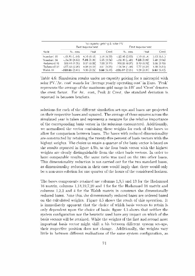
No capacity pricing & solar PVBest improvement First improvement

Basis Av. cost Peak Crest Av. cost Peak Crest

Standard 16 -161.87 (1.04) 8.76 (0.46) 5.76 (0.30) -122.46 (2.63) 7.70 (0.18) 5.13 (0.11)Standard 24 -134.30 (0.85) 7.88 (0.36) 5.85 (0.24) -101.00 (1.48) 7.23 (0.09) 5.40 (0.04)Hadamard 16 -333.44 (2.76) 9.32 (0.39) 2.93 (0.12) -203.68 (0.97) 9.19 (0.29) 3.86 (0.10)Hadamard 24 -277.33 (2.26) 8.56 (0.39) 3.64 (0.15) -150.58 (1.38) 7.77 (0.29) 4.40 (0.13)Walsh 16 -333.95 (2.87) 9.30 (0.22) 2.86 (0.10) -221.07 (2.27) 9.28 (0.39) 3.65 (0.12)

Table 4.6: Simulation results under no capacity pricing for a microgrid withsolar PV.'Av. cost' stands for 'Average yearly operating cost' in Euro. 'Peak'represents the average of the maximum grid usage in kW and 'Crest' denotesthe crest factor. For Av. cost, Peak & Crest, the standard deviation isreported in between brackets.

solutions for each of the di�erent simulation set-ups and bases are projectedon their respective bases and squared. The average of these squares across thesimulated year is taken and represents a measure for the relative importanceof the corresponding basis vector in the solutions encountered. Additionally,we normalised the vector containing these weights for each of the bases toallow for comparison between bases. The bases with reduced dimensionalityare constructed by retaining the twenty-�ve percent of basis vectors with thehighest weights. The choice to retain a quarter of the basis vector is based onthe results reported in �gure 4.5b, as the four basis vector with the highestweights are clearly distinguishable from the other basis vectors. In order tohave comparable results, the same ratio was used on the two other bases.This dimensionality reduction is not carried out for the two standard bases,as dimensionality reduction in their case would imply that there would onlybe a non-zero solution for one quarter of the hours of the considered horizon.

The bases components retained are columns 1,9,5 and 13 for the Hadamard16 matrix, columns 1,13,19,7,20 and 4 for for the Hadamard 16 matrix andcolumns 1,2,3 and 4 for the Walsh matrix in construct the dimensionallyreduced bases. Note that the dimensionally reduced bases are ordered basedon the calculated weights. Figure 4.5 shows the result of this operation. Itis immediately apparent that the choice of which basis vectors to retain isonly dependent upon the choice of basis: �gure 4.5 shows that neither thesystem con�guration nor the heuristic used have any impact on which of thebasis vectors will be retained. While the weights of the �rst and second mostimportant basis vector might shift a bit between di�erent system set-ups,their respective position does not change. Additionally, the weights varylittle in between di�erent realisations of the same system con�guration, as

74

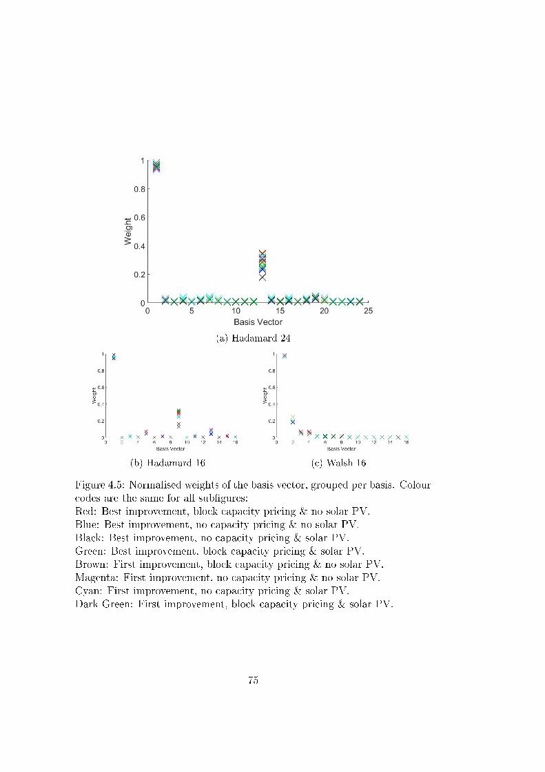
(a) Hadamard 24

(b) Hadamard 16 (c) Walsh 16

Figure 4.5: Normalised weights of the basis vector, grouped per basis. Colourcodes are the same for all sub�gures:Red: Best improvement, block capacity pricing & no solar PV.Blue: Best improvement, no capacity pricing & no solar PV.Black: Best improvement, no capacity pricing & solar PV.Green: Best improvement, block capacity pricing & solar PV.Brown: First improvement, block capacity pricing & no solar PV.Magenta: First improvement, no capacity pricing & no solar PV.Cyan: First improvement, no capacity pricing & solar PV.Dark Green: First improvement, block capacity pricing & solar PV.

75

the marks of the same colour are superimposed on one another in �gure 4.5.

4.3.3 Results with dimensionality reduction

In order to evaluate the impacts of using these dimensionally reduced baseson the yearly operational cost, the experiments were rerun using the dimen-sionally reduced bases. The scenario without a capacity tari� was not sim-ulated again because of the high externalities that resulted from this scenario.

As is immediately apparent from comparing the results reported in tables 4.7to 4.10 with their respective counterparts without dimensionality reduction,the performance of the heuristics after dimensionality reduction is highlydependent on the simulation set-up. Whereas the heuristics using the di-mensionality reduced bases outperform the full dimensionality bases for thecase of a system without PV operating under a block capacity tari� scheme,and almost reach the same performance for a system without PV operatingunder �xed capacity tari�s. In both simulation set-ups incorporating solarPV, the dimensionally reduced bases are outperformed by the heuristics us-ing the full dimensionality bases.

As can be seen from tables 4.7 and 4.9, the heuristics using the dimensionallyreduced bases manage to keep the peak capacity usage down, tables 4.8 and4.10 show a similar, but less pronounced, reduction of peak capacity usagefor the system con�gurations with solar PV generation. The crest factorsexhibit a similar behaviour.

Looking at the results for the dimensionally reduced bases, it is now theWalsh base that presents the low average cost overall, being the cheapest insix out of eight of the simulation con�gurations ran, while being well within 1standard deviation from the best performing algoritm in the two other cases.This reversal from the results discussed in section 4.3.1 shows that the Walsh16 basis is the most suited of the bases for the dimensionality reduction out-lined above.

The main reason for the higher yearly operating costs prevalent amongst theheuristics using the dimensionally reduced bases is that they no longer havethe �exibility to fully make use of the arbitrage operations o�ered by thereal-time energy market, precisely because of the reduction of dimensionalityin the bases used. These higher average yearly operating costs are howevero�set by a reduction in computation time: while comprehensive and compar-able data on runtimes is not available as the simulations were run in parallel

76

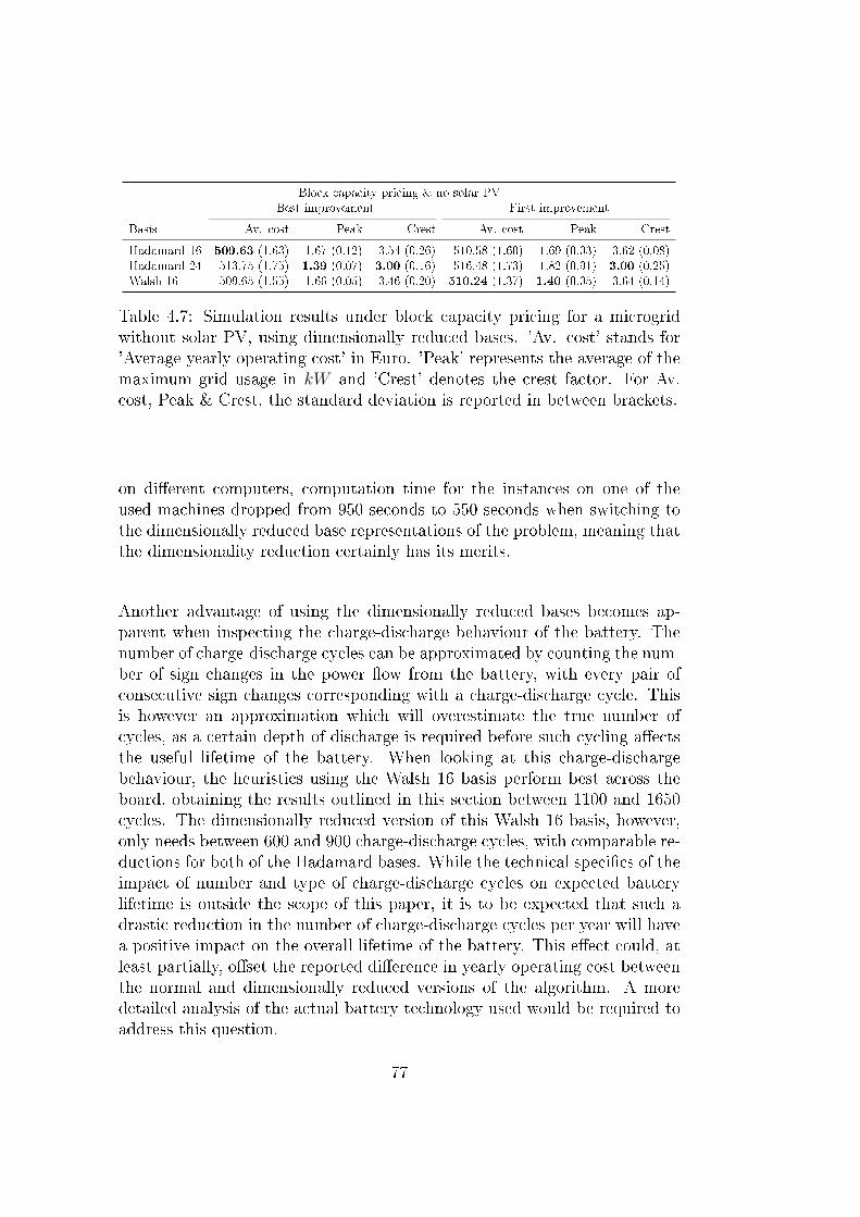
Block capacity pricing & no solar PVBest improvement First improvement

Basis Av. cost Peak Crest Av. cost Peak Crest

Hadamard 16 509.63 (1.63) 1.67 (0.12) 3.54 (0.26) 510.58 (1.60) 1.69 (0.03) 3.62 (0.08)Hadamard 24 513.75 (1.75) 1.39 (0.07) 3.00 (0.16) 516.48 (1.73) 1.82 (0.91) 3.00 (0.25)Walsh 16 509.65 (1.55) 1.66 (0.05) 3.46 (0.20) 510.24 (1.37) 1.40 (0.05) 3.64 (0.14)

Table 4.7: Simulation results under block capacity pricing for a microgridwithout solar PV, using dimensionally reduced bases. 'Av. cost' stands for'Average yearly operating cost' in Euro. 'Peak' represents the average of themaximum grid usage in kW and 'Crest' denotes the crest factor. For Av.cost, Peak & Crest, the standard deviation is reported in between brackets.

on di�erent computers, computation time for the instances on one of theused machines dropped from 950 seconds to 550 seconds when switching tothe dimensionally reduced base representations of the problem, meaning thatthe dimensionality reduction certainly has its merits.

Another advantage of using the dimensionally reduced bases becomes ap-parent when inspecting the charge-discharge behaviour of the battery. Thenumber of charge-discharge cycles can be approximated by counting the num-ber of sign changes in the power �ow from the battery, with every pair ofconsecutive sign changes corresponding with a charge-discharge cycle. Thisis however an approximation which will overestimate the true number ofcycles, as a certain depth of discharge is required before such cycling a�ectsthe useful lifetime of the battery. When looking at this charge-dischargebehaviour, the heuristics using the Walsh 16 basis perform best across theboard, obtaining the results outlined in this section between 1100 and 1650cycles. The dimensionally reduced version of this Walsh 16 basis, however,only needs between 600 and 900 charge-discharge cycles, with comparable re-ductions for both of the Hadamard bases. While the technical speci�cs of theimpact of number and type of charge-discharge cycles on expected batterylifetime is outside the scope of this paper, it is to be expected that such adrastic reduction in the number of charge-discharge cycles per year will havea positive impact on the overall lifetime of the battery. This e�ect could, atleast partially, o�set the reported di�erence in yearly operating cost betweenthe normal and dimensionally reduced versions of the algorithm. A moredetailed analysis of the actual battery technology used would be required toaddress this question.

77

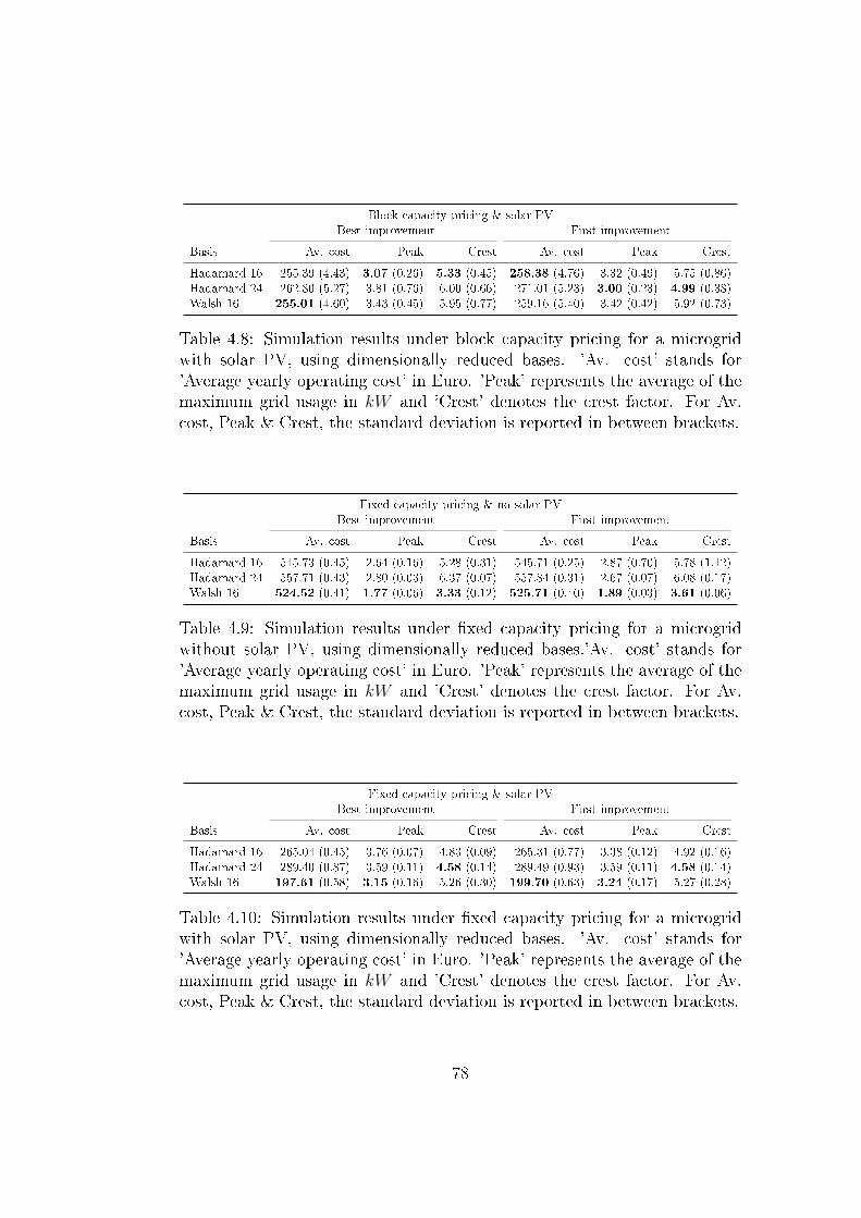
Block capacity pricing & solar PVBest improvement First improvement

Basis Av. cost Peak Crest Av. cost Peak Crest

Hadamard 16 255.39 (4.43) 3.07 (0.26) 5.33 (0.45) 258.38 (4.76) 3.32 (0.49) 5.75 (0.86)Hadamard 24 262.80 (5.27) 3.81 (0.76) 6.00 (0.66) 271.01 (5.23) 3.00 (0.23) 4.99 (0.38)Walsh 16 255.01 (4.60) 3.43 (0.45) 5.95 (0.77) 259.16 (5.40) 3.42 (0.42) 5.92 (0.73)

Table 4.8: Simulation results under block capacity pricing for a microgridwith solar PV, using dimensionally reduced bases. 'Av. cost' stands for'Average yearly operating cost' in Euro. 'Peak' represents the average of themaximum grid usage in kW and 'Crest' denotes the crest factor. For Av.cost, Peak & Crest, the standard deviation is reported in between brackets.

Fixed capacity pricing & no solar PVBest improvement First improvement

Basis Av. cost Peak Crest Av. cost Peak Crest

Hadamard 16 545.73 (0.45) 2.64 (0.16) 5.28 (0.31) 545.71 (0.25) 2.87 (0.70) 5.78 (1.42)Hadamard 24 557.71 (0.43) 2.80 (0.03) 6.37 (0.07) 557.84 (0.31) 2.67 (0.07) 6.08 (0.17)Walsh 16 524.52 (0.41) 1.77 (0.06) 3.33 (0.12) 525.71 (0.40) 1.89 (0.03) 3.61 (0.06)

Table 4.9: Simulation results under �xed capacity pricing for a microgridwithout solar PV, using dimensionally reduced bases.'Av. cost' stands for'Average yearly operating cost' in Euro. 'Peak' represents the average of themaximum grid usage in kW and 'Crest' denotes the crest factor. For Av.cost, Peak & Crest, the standard deviation is reported in between brackets.

Fixed capacity pricing & solar PVBest improvement First improvement

Basis Av. cost Peak Crest Av. cost Peak Crest

Hadamard 16 265.04 (0.45) 3.76 (0.07) 4.83 (0.09) 265.31 (0.77) 3.38 (0.12) 4.92 (0.16)Hadamard 24 289.40 (0.87) 3.59 (0.11) 4.58 (0.14) 289.49 (0.93) 3.59 (0.11) 4.58 (0.14)Walsh 16 197.61 (0.58) 3.15 (0.16) 5.26 (0.30) 199.70 (0.63) 3.24 (0.17) 5.27 (0.28)

Table 4.10: Simulation results under �xed capacity pricing for a microgridwith solar PV, using dimensionally reduced bases. 'Av. cost' stands for'Average yearly operating cost' in Euro. 'Peak' represents the average of themaximum grid usage in kW and 'Crest' denotes the crest factor. For Av.cost, Peak & Crest, the standard deviation is reported in between brackets.

78

4.4 Conclusion

We have solved the day-ahead economic dispatch problem for a microgridwith storage and local intermittent generation and with the inclusion of ca-pacity tari�s. We used our own multi-start heuristic to solve this problem,and showed our heuristic approach to be e�ective. Our results have bothmethodological and policy implications.

Where the methodology is concerned, our results show that using a rep-resentation which mimics some of the periodicity inherently present in theproblem being studied has bene�ts, as evidenced by the strong performanceof the non-standard bases used. Furthermore, we have shown that thesenon-standard bases can be used to reduce the dimensionality of the prob-lem, thereby saving on computational time: a dimensionality reduction of75% corresponded to a runtime reduction of 40% and a cost increase of 20%,clearly showing that the dimensionality reduction has merit.

We have also shown how it is possible to steer consumer load with both en-ergy and capacity price signals. Our results show the impact of the design ofthe capacity tari� on the load behaviour of consumers: a block capacity tari�is able to limit peak capacity usage more than a �xed capacity tari� scheme,which is in accordance with the results earlier published by Fridgen et al. [9],while at the same time leading to comparable cost outcomes for the consumer.

Finally, our results show that the balance between the energy price andthe capacity price for electricity is important, and impacts both the yearlyoperation cost of the individual microgrid, as well as the peak capacity usage,meaning that this is a worthwhile avenue of further research.

79

80

Bibliography

[1] IEEE Smartgrid [Internet], IEEE joint task force on quadrennial en-ergy review, Utility and Other Energy Company Business Case IssuesRelated to Microgrids and Distributed Generation (DG), EspeciallyRooftop Photovoltaics, Presentation to the U.S. Department of Energy2014, on the www, url:https://smartgrid.ieee.org/images/files/pdf/IEEE\_QER\_Microgrids\\\_October\_3\_2014.pdf.

[2] A. Cagnano, A. Caldarulo Bugliari, E. De Tuglie A cooperative con-trol for the reserve management of isolated microgrids, Applied Energy2018;218;256-265.

[3] Quashie M., Marnay C., Bou�ard F., Joós G. Optimal planningof microgrid power and operating reserve capacity, Applied Energy2018;210;1229-1236.

[4] Makrygiorgou D., Alexandridis A. Distributed stabilizing modular con-trol for stand-alone microgrids, Applied Energy 2018;210; 925-935

[5] Cucuzzella M., Lazzari R., Trip S., Rosti S., Sandroni C., Ferrara A.Sliding mode voltage control of boost converters in DC microgrids, Con-trol Engineering Practice 2018;Volume 73;161-170.

[6] Mengelkamp E., Gärttner J., Rock K., Kessler S., Orsini L., WeinhardtC. Designing microgrid energy markets: A case study: The BrooklynMicrogrid, Applied Energy 2018;210;870-880.

[7] Ahmad F., Alam M. S. Economic and ecological aspects for microgridsdeployment in India, Sustainable Cities and Society 2018;37;407-419.

[8] Milis K., Peremans H., Van Passel S. The impact of policy on mi-crogrid economics: A review, Renewable and Sustainable Energy Re-views 2018;81.2;3111-3119.

81

[9] Fridgen G., Kahlen M., Ketter W., Rieger A., Thimmel M. One ratedoes not �t all: An empirical analysis of electricity tari�s for residentialmicrogrids, Applied Energy 2018;210;800-814.

[10] DeForest N., Jason S. MacDonald J.S?, Douglas R. Black D. R. Dayahead optimization of an electric vehicle �eet providing ancillary ser-vices in the Los Angeles Air Force Base vehicle-to-grid demonstration,Applied Energy 2018;210;987-1001.

[11] Liu F., Bie Z., Liu S., Ding T. Day-ahead optimal dispatch for windintegrated power system considering zonal reserve requirements, AppliedEnergy 2017;188;399-408.

[12] Crowston, W.B., Glover, F., Thompson, G.L., Trawick, J.D., 1963.Probabilistic and Parametric Learning Combinations of Local Job ShopScheduling Rules. Technical Report 117. Carnegie-Mellon University,Pittsburgh.

[13] Muth, J.F., Thompson, G.L., 1963. Industrial Scheduling. Prentice-Hall

[14] Hansen, P., Mladenovi¢ N. First vs. best improvement: An empiricalstudy, Discrete Applied Mathematics 2006;154;802-817.

[15] Ochoa G., Verel S., Tomasssini M. Frist-improvment vs. Best-improvement Local Optima Networks of NK lanscapes, Parallel ProblemSolving From Nature 2010;104-113.

[16] Synergrid, Synthetic Load Pro�les (SLP) , on the www,http://www.synergrid.be/index.cfm?PageID=16896, last consultedon 15/09/2017 (in Dutch)

[17] Belpex, 2017Market Data Services, September. On the www, url:https://www.belpex.be/servies/market-data-services.

[18] Elia, 2014. Solar-PV Power Generation Data, October. On the WWW,url: http://www.elia.be/en/grid-data/power-generation/

Solar-power-generation-data.

[19] Schreiber M, Wainstein ME, Hochlo� P, Dargaville R. Flexible electri-city tari�s: Power and energy price signals designed for a smarter grid,Energy 2015; 93;2568-2581.

82

Appendix A: Linear algebra and intuition be-

hind di�erent bases

A basis is a linearly independent spanning set of vectors. Linearly inde-pendent means that it is impossible to write one of the vectors as a linearcombination of the other vectors in the set, while spanning means that allthe vectors in the considered vector space can be expressed as a linear com-bination of the considered set of vectors. As an example, consider R2, thevector space of all coordinates (a, b) where both a and b are real numbers.The standard basis for R2 is e1 = (1, 0) and e2 = (0, 1). Take for instancethe vector 2 = (2, 2), it is easy to see that v = 2 ·e1 +2 ·e2. However, anothervalid basis for R2 is f1 = (1, 1) and f2 = (1,−1); it is easy to see that thesetwo vectors are linearly independent, and it has been proven that a linearlyindependent set of dimension n is a basis for an n dimensional vector space,meaning that the spanning property need not be proven. The vector v cannow also be written as v = 2 · f1 + 0 · f2. Note that the vector v has notchanged, it are only the coordinates that are used to describe the vector inrelation to the basis vectors that are dependent on the choice of basis vectors.

e1

e2

v

f1

f2

Two di�erent two dimensional bases

Now, consider an extension of this two dimensional example to a four di-mensional vector space. However, instead of looking at an arbitrary fourdimensional space, let us apply this to a rudimentary load pro�le. This loadpro�le splits a complete day into four di�erent, 6 hour sections: �1: morn-ing� (06.00-12.00), �2: afternoon� (12.00-18.00), �3: evening� (18.00-00.00)and �4: night� (00.00-06.00). In order to now fully describe a load pro�le

83

of this kind, it is enough to know how high the load is for the four di�erentperiods, hence the four dimensional space. Just as in the previous example,the standard basis for this four dimensional space is e1 = (1, 0, 0, 0), e2 =(0, 1, 0, 0), e3 = (0, 0, 1, 0) and e4 = (0, 0, 0, 1). So, a load pattern, l1, thatuses 4 units (dimensionless, for ease of discussion) of power in the morn-ing, 4 units during the afternoon, 2 units during the evening and 2 unitduring the night is l1 = 4 · e1 + 4 · e2 + 2 · e3 + 2 · e4. However, just asbefore, it is also possible to de�ne other bases for this four dimensional vec-tor space, like the walsh basis: w1 = (1, 1, 1, 1), w2 = (1, 1,−1,−1), w3 =(1,−1,−1, 1), w4(1,−1, 1,−1). l1 can now also be expressed in terms of thewalsh basis: l1 = 3 ·w1 + 1 ·w2 + 0 ·w3 + 0 ·w4. Note how in this example itis possible to assign meaning to the di�erent basis vectors: in the case of thestandard basis, each of the basis vectors captures the height of the load pro�leduring the corresponding hour. When looking at the Walsh basis, however,each of the basis vectors can be understood as a certain trend within the loadpro�le: the �rst basis vector models the base load, as it is a constant term,while the second component encodes for a pro�le with a higher load duringthe daytime periods, and a lower load during night time periods. Similarly,the third and fourth basic vectors are patterns showing a similar, periodicvariation.

Load

Period1 2 3 4

1

2

-1

-2

e1

Load

Period1 2 3 4

1

2

-1

-2

e2

Load

Period1 2 3 4

1

2

-1

-2

e3

Load

Period1 2 3 4

1

2

-1

-2

e4

Standard Basis

84

Load

Period1 2 3 4

1

2

-1

-2

w1

Load

Period1 2 3 4

1

2

-1

-2

w2

Load

Period1 2 3 4

1

2

-1

-2

w3

Load

Period1 2 3 4

1

2

-1

-2

w4

Walsh Basis

The reason to explore such a non-standard basis, like the Walsh basis is ap-parent from the example outlined before: assuming that there is some peri-odic behavior apparent in the set of vectors that we want to study, it might beeasier to represent them as a sum of certain periodic basis components thanas a sum of what happens on each of the individual series considered. Fur-thermore, based on our hypothesis that some of these periodic componentswill be more important for the set of vectors we are interested in, the Walshrepresentation allows those vectors to be represented using only a subset ofthe original basis vectors. The simpli�ed, intuitive, example is as follows:assume that that the vector l1 is the pattern corresponding to the optimalsolution to the optimization problem outlined in section 4.2.1; if we searchfor this solution using the standard basis, we need all four basis vectors tobe able to construct l1. However, if we search for this solution using theWalsh basis, two of the four basis vectors su�ce for the construction of l1.Of course, this line of reasoning is only true if most of the optimal solu-tions contain certain patterns, corresponding to certain basic vectors, morestrongly than other. However, �gure 4.5 presented in section 4.3.2 show thatthis is the case for the problem being studied within.

85

86

Chapter 5

Steering the adoption of battery

storage through electricity tari�

design1

Abstract

The economic viability of electricity storage using batteries, under di�erenttari� structures and system con�gurations, is investigated. The economicoutcomes of the di�erent combinations of tari� design and system con�g-uration are evaluated. Based on a discussion of the relevant literature, thefollowing tari� designs are used in the study: (i) �xed energy prices, (ii)real-time energy pricing, (iii) �xed rate capacity tari�s, and (iv) capacity de-pendent capacity tari�s. Next, the di�erent simulated system con�gurationsare outlined: (i) no battery storage, (ii) battery storage only, and (iii) batterystorage and decentralized renewable energy production with PV. Our studyprovides insights for policy makers, showing that capacity block pricing onlyincentivises storage as part of an (existing) PV installation, while the com-bination of real time energy pricing and capacity block pricing promotes awider adoption of battery storage.

5.1 Introduction

Smart grids have been widely researched as a possible solution for the decar-bonisation of society's electricity demand, by allowing a greater penetration

1This chapter has been submitted for publication to Renewable and Sustainable Energy

Reviews as Milis, K., Peremans, H., Van Passel S. Steering the adoption of battery storage

through electricity tari� design

87

of renewable energy sources [1],[2],[3]. One possibility to arrive at such a lowcarbon smart grid, is the adoption of so-called microgrids. A microgrid iswidely understood to be a grouping of electrical as well as heat loads andsources, being able to operate either in self-contained, islanded mode, or aspart of the distribution system, in which case a microgrid is to act as a single,controllable load [4],[5],[6],[7]. This of course raises the question of how suchloads should be controlled, a discussion of standardisation and control prin-ciples in can be found in [8], speci�cally aimed at controlling the load thatmicrogrids represent.

A good overview of the drivers behind and challenges facing microgrids isgiven in [9], [10] zooms in on the challenges and opportunities concerningsmart grids and microgrids. In previous work [11], it has been shown thatthere is a dearth of research looking at the policy impacts of di�erent tari�schemes on the economics of microgrids, as most tari� policy research fo-cusses on the utilities.

One main recurring component which has been widely investigated in thecontext of microgrids, is storage, both of heat and electricity. Storage is awell-researched component, as it greatly facilitates balancing of generationand load. As shown in [12], locally available storage allows for e�cient con-trol of the grid through the use of well-designed price signals. However, asuitable and robust business case for storage remains elusive, as evidenced byvarious publications looking at di�erent possibilities: using the battery capa-city of electric vehicles in a vehicle-to-grid setup was investigated by in [13],while [14] investigates the possibility of using arbitrage possibilities. Bothpapers report favourable outcomes in some, but not all, scenarios. Furtherevidence of the precarious business case underpinning the adoption of storageis provided in [15], showing that round trip e�ciency and capital costs -bothdrivers for the overall cost of ownership- are still signi�cant barriers to thewide scale adoption of energy storage technologies.

Against this backdrop of proven societal bene�ts from the adoption of stor-age on the one hand and uncertain pro�tability on the other hand, this pa-per investigates the impact of government policy on the adoption of energystorage. More speci�cally, we look at the impact of a capacity tari� for elec-tricity on the household adoption of battery storage. In order to e�ectuatethis analysis, we simulate di�erent household microgrid con�gurations undervarying electricity price and tari� schemes, minimizing the total operationalcost over the period of one year for a modal residential Belgian consumer. .The choice of nationality is driven by ease of access to the relevant data; as

88

the authors are attached to a publicly funded Belgian university, the Belgiantransmission and distribution system operators readily made the requireddata available. As systems costs and technical performance of intermittentgeneration and storage are not only the subject of signi�cant technologicalchange but also important drivers of the overall pro�tability of any given mi-crogrid con�guration [15], no a priori assumptions are made when it comesto installation costs or technical performance of intermittent generation orstorage. The analysis made will instead indicate the tipping point, expressedas an annualized cost below which di�erent systems con�gurations becomeeconomically viable.

The following section provides a more in depth literature review concern-ing the issues of interest directly linked to the research question at hand.Section three states the research goal as well as the central research hypo-thesis, thereby also clearly delineating the contribution of this work. Thefourth section details the research methodology used, and discusses in orderthe research method, the research variables and the design of the simulationmodel. A presentation of results and a discussion of these results and policyimplications closes this paper.

5.2 Literature review

Research into microgrids is fertile �eld, as evidenced by the comprehensiveliterature review establishing a functional layer based classi�cation [16]. Thisreview provides a good starting point and provides a broad overview of mi-crogrid concepts as well as existing microgrid test beds. As [16] providesa good basis of information, the remainder of this section will be explicitlyfocused on the areas of interest of this paper, being policy measures used toin�uence system con�guration on the one hand, and microgrid modeling andsimulation on the other hand.

As mentioned in the introduction, little research has been done on the im-pact of policy on microgrid economics [11]. A popular investigated policyintervention is carbon taxation, as it is present in a majority of earlier work[17, 18, 19, 20, 21, 22]. The reported results of this policy intervention aremixed however: either they result in no noticeable impact on the microgrid,compared to the no intervention scenario [17, 18, 22] or they incentivise theinstallation of solar PV, but only when combined with a feed-in tari� forelectricity generated by these panels [19, 20]. Only one case reports a some-what favourable outcome of carbon taxation where renewable generation is

89

concerned [21].

As already outlined above, economic incentives in the form of feed in tari�scan be e�ective [19, 20], while su�ciently high tax credit, amounting to 50%of the installation cost in [22], will have a signi�cant impact on the installedsystem con�guration, heavily favouring the adoption of wind power. Whenthe operation of the installed system is considered as well, the results aremore mixed: conventionally �red CHP units still contribute the majority ofthe generated power in the system modelled in [22], while some of the con-sidered feed-in tari�s are higher than the grid price of electricity, leading tothe system buying all needed power from the grip, while selling all generatedpower from the solar panels at the same time.

Less work has been done on investigating the impact of di�erent tari� sys-tems, and the work available focuses exclusively on energy time of use pricing,however, once again, the impact is found to be negligible [18], or sometimeseven negative, if emission costs are considered [23].

Time of use pricing is generally more studied as a measure to steer consumerloads [24], without taking the resulting economics into account [25]. Alonga similar vein is the work presented in [12], capacity instead of energy pricesignals are used to steer a controllable load. The choice for using capacitypricing as a signal as opposed to energy pricing is made because this betterre�ects the economic realities distribution system operators are faced with,when serving the connected consumer loads. Furthermore, these measuresare found to be e�ective in their stated goal of steering consumer loads.

There is a broad consensus in existing research where the simulation andmodelling of microgrids is concerned: simulations are set-up and mathemat-ical optimisation based on mixed integer programming is carried out [17, 22].The scope of di�erent presented models in the literature di�ers however: somemodels are operational models, focusing exclusively on operational paramet-ers [18], while others are investment models, taking both the investment andoperational costs into account [17, 19, 20].

5.3 Research goal & hypothesis

Based on the review outlined above in section 2 and the �ndings reportedin [11] a clear research gap becomes evident: to the best of the author's

90

knowledge there has been no research focusing on using capacity tari�s toencourage the uptake of storage technologies. The contribution of this paperis that it closes that research gap, by presenting the impacts of a capacitytari� scheme, both by itself as well as in conjunction with real time energypricing and evaluating the impact of these pricing schemes on a residentialmicrogrid. In doing so, this paper not only extends the breadth of scienti�cknowledge surrounding microgrids, but also expands the toolkit of policy-makers, by providing evidence of the impact of capacity tari�s on the eco-nomics of di�erent microgrid system con�gurations.

The above contribution translates itself to the following research hypothesis:capacity tari�s will be e�ective in di�erentiating between di�erent systemcon�gurations, where the economics of these di�erent systems are concerned,speci�cally favouring system con�gurations including storage. The reason-ing behind this hypothesis is that system with storage will be able to engagebetter in peak-shaving behaviour, allowing them to avoid the higher costsincurred for high peak usage of capacity. This hypothesis will be tested bysimulating di�erent system con�gurations -with and without storage as wellas with and without intermittent generation-, under a no intervention sce-nario, a scenario with capacity tari�s, and a scenario with both capacitytari�s and real time energy pricing. This research aligns itself with thosepapers taking an operational approach, deliberately choosing not to take in-vestment cost into account, but instead aiming to provide policy insightsthat are relevant regardless of the current installation costs of the investig-ated technologies.

5.4 Research Methodology

This section discusses in detail the methodology used to test the hypothesisoutlined in section 3. A �rst subsection details the research method used,detailing both the simulation model as well as the optimisation problem be-ing solved. The second subsection delves deeper into the policy interventionsinvestigated, while the third and �nal subsection elaborates on the particu-lars of the simulations.

91

Grid

Load

Storage+Qg +Qs

+Ql

(a) Model without intermittent generation

Grid

Load

Storage+Qg +Qs

+Ql

Inter-mittent

+Qi

(b) Model with intermittent generation

Figure 5.1: Model con�gurations

5.4.1 Reserach method

In order to investigate the impact of electricity tari� design on the adop-tion of battery storage, a simulation model is used. The model used is are�nement of the model presented in [26]: a residential consumer is mod-elled, consisting at a minimum of an exogenous load pro�le and a connectionto the electricity grid, which serves as a limitless source or sink of electricalenergy. Additionally, local distributed generation and/or storage can also bepresent. The model only incorporates electrical generation and load, heat isnot included. As more fully elaborated upon in [26], the explicit focus of themodel is the underlying economics, meaning abstraction is made of technicalconsiderations such as line losses or most of the technical aspects of individualmodel components. Figures 5.1a and 5.1b present a schematic overview ofthe used model: �gure 5.1a shows the modeled system without the presenceof intermittent generation, while �gure 5.1b shows the system layout for thecase where intermittent generation is included in the modeled system. Addi-tionally, both �gures 5.1a and 5.1b also show the sign convention used: powerand energy �ows are considered positive when they are �owing towards theload. While this results in the seemingly counter-intuitive situation wherecharging the storage component means a negative sign for the respectiveterm, Qs, this sign convention was chosen to ensure consistency across all ofthe terms used in the equation.

For the simulated system, the yearly operating cost, comprised of the pay-ments made for the used energy and applicable tari�s, is minimized using

92

Matlab. The formulation of the problem is as follows (please consult thenomenclature at the end of this paper for the meaning of the used symbols).We minimize the cost function

minQG

[24∑t=1

QG(t) · PG(t) + |QG(t)| · Cp1 +max (|QG(t)| − Cb, 0) · (Cp2 − Cp1)

](5.1)

subject to the following constraints:

QL(t) = QG(t) +QS(t) +QI(t) ∀t = 1, ..., 24 (5.2)

Sin(1)−t∑

τ=1

QS(τ) 6 Smax ∀t = 1, ..., 24 (5.3)

t∑τ=1

QS(τ) 6 Sin(1) ∀t = 1, ..., 24 (5.4)

The decision variables used in the simulation model is the vectorQG (t) withthe index t running over a 24-hour period. At the start of each 24-hourperiod, we renumber the indexes of the hours considered, so that the �rsthour has index 1, and the last hour has index 24. A rolling 24-hour window isused: after the optimization is �nished for the �rst 24 hours, the solution forthe �rst hour is saved, after which the optimization is carried out for hours2 through 25, yielding the solution for the second hour, and so on and so forth.

Before elaborating on the cost function and the constraints, it is importantto discuss the sign convention used. All �ows of power to the load are posit-ive, while all �ows of power away from the load are negative, by convention.This does not impact QI as the amount of power available from the distrib-uted generation will always be non-negative. However, said sign conventionhas some repercussions where the interpretation of the signs of the decisionvariables, QG and QS are concerned. For QG, this simply means that powerbought from the grid will have a positive sign, while power sold to the gridwill have a negative sign. It is especially important to keep the sign conven-tion in mind with regards to QS, as charging storage will be re�ected by anegative value of QS, while discharging power from storage will result in apositive sign for QS.

Equation 5.1 details the cost function to be minimized and has two com-ponents. The �rst component contains the cost for electricity used from thegrid �or, conversely, the bene�t realised by selling electricity to the grid�,

93

while the second component represents payments made to the grid operatorfor the grid capacity used. It should be noted that the actual payments arecalculated using a block tari� scheme, where all capacity used above a certainlevel, Cb, has to be remunerated at a higher tari�.

For each time-step considered, i.e. for each value of index t, the sum of theamount withdrawn from the grid, the amount withdrawn from storage andthe power available from the intermittent generation must be equal to theload that needs to be served; this is enforced by equation 5.2. Equations 5.3and 5.4 are two sets of constraints on the battery: equations 5.3 enforces thatthe battery can never be charged past its fully charged state, while equations5.4 states that the battery cannot be further discharged when it is alreadyempty. These are two sets of twenty-four equations each, as they have to bemet for each hour of the 24-hour modeling window.

The resolution used in the simulation set-up is one data point per hour. Thismeans that all the variables considered are to be read as energy amounts.However, as one of the main aims of this paper is to investigate the impactof capacity tari�s, capacity used is also included: electricity bought or soldduring each hour is assumed to be uniformly distributed over that hour,which means that the peak capacity during that hour also corresponds tothe electricity bought or sold. For example, assume that during a certainhour, 1.5 kWh of electricity was bought from the grid, this corresponds toa capacity usage of 1.5 kW during the entirety of this one-hour window,resulting in a peak capacity usage of, again, 1.5 kW for the hour underconsideration. Consecutive hours are linked through the storage component,as the amount of energy in storage at the end of time-step t, is also theamount of energy that will be in the storage component at the start of time-step t+1. With the addition of time-varying energy prices, as is the casefor some simulations setups discussed below, this linkage through the energystored in the storage component, causes the system to become a non-causalone, as the optimal decision at any given moment is dependent on futureevents. The modelling intricacies this entails are further discussed in [26].

5.4.2 Reseerach variables

In this study, the household electricity bill is split into two parts, an en-ergy component and a capacity component. The energy component providesremuneration for the energy provider and can either be a re�ection of the�uctuating wholesale market price, or �xed rate per kWh consumed. Inthe studied Belgian setting, household electricity consumers are currently

94

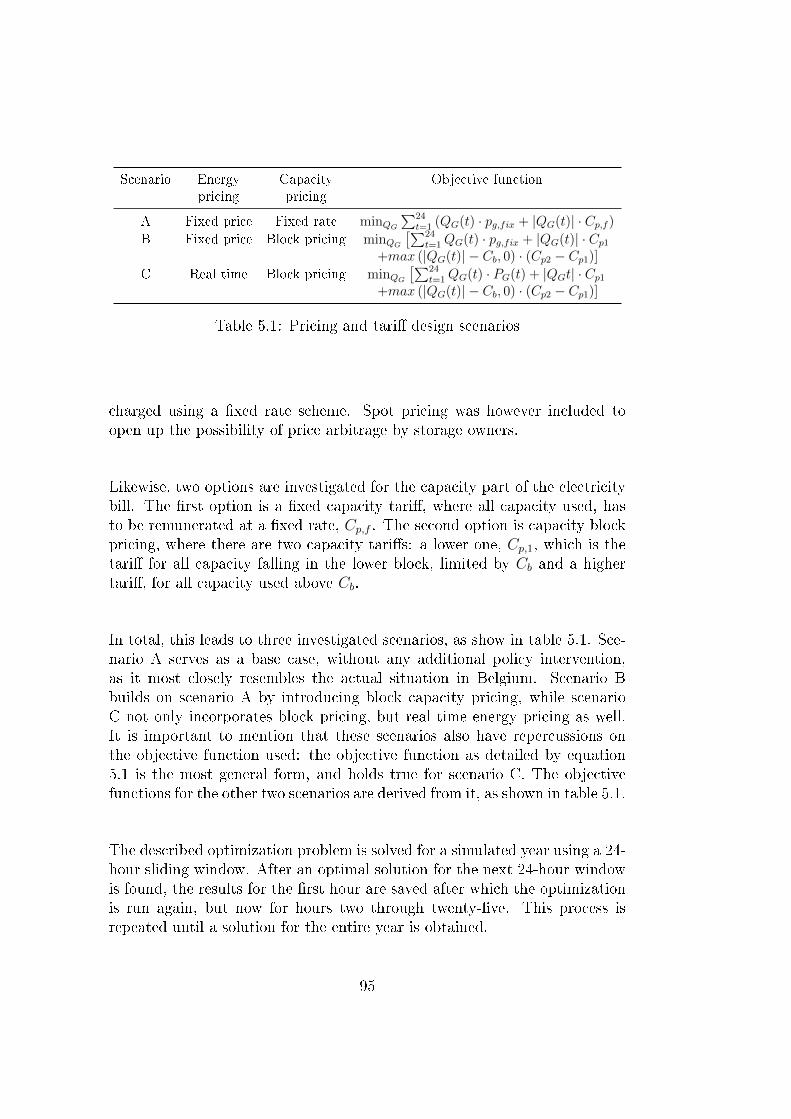
Scenario Energy Capacity Objective functionpricing pricing

A Fixed price Fixed rate minQG

∑24t=1 (QG(t) · pg,fix + |QG(t)| · Cp,f )

B Fixed price Block pricing minQG

[∑24t=1QG(t) · pg,fix + |QG(t)| · Cp1

+max (|QG(t)| − Cb, 0) · (Cp2 − Cp1)]C Real time Block pricing minQG

[∑24t=1QG(t) · PG(t) + |QGt| · Cp1

+max (|QG(t)| − Cb, 0) · (Cp2 − Cp1)]

Table 5.1: Pricing and tari� design scenarios

charged using a �xed rate scheme. Spot pricing was however included toopen up the possibility of price arbitrage by storage owners.

Likewise, two options are investigated for the capacity part of the electricitybill. The �rst option is a �xed capacity tari�, where all capacity used, hasto be remunerated at a �xed rate, Cp,f . The second option is capacity blockpricing, where there are two capacity tari�s: a lower one, Cp,1, which is thetari� for all capacity falling in the lower block, limited by Cb and a highertari�, for all capacity used above Cb.

In total, this leads to three investigated scenarios, as show in table 5.1. Sce-nario A serves as a base case, without any additional policy intervention,as it most closely resembles the actual situation in Belgium. Scenario Bbuilds on scenario A by introducing block capacity pricing, while scenarioC not only incorporates block pricing, but real time energy pricing as well.It is important to mention that these scenarios also have repercussions onthe objective function used: the objective function as detailed by equation5.1 is the most general form, and holds true for scenario C. The objectivefunctions for the other two scenarios are derived from it, as shown in table 5.1.

The described optimization problem is solved for a simulated year using a 24-hour sliding window. After an optimal solution for the next 24-hour windowis found, the results for the �rst hour are saved after which the optimizationis run again, but now for hours two through twenty-�ve. This process isrepeated until a solution for the entire year is obtained.

95

Cp,f 0.0652 e/kWCp,1 0.0581 e/kWCp,2 0.1872 e/kW

Table 5.2: Capacity prices

5.4.3 Design of the simulation model

Following the elaboration on the used simulation framework in the previoussection, this subsection provides greater detail on the design of the investig-ated policy interventions on the one hand, and the simulated system con�g-urations on the other hand. Furthermore, the used data sources and instancegeneration are also discussed.

Energy and capacity price points

As Schreiber et al. report favourable results with such capacity tari� designin [12], the same values for Cp,f , Cp,1 and Cp,2 are used as starting points inthis study. The numerical values of these parameters can be found in table5.2.

Since the overall goal of the capacity block tari�s is to reduce the peak loadon the system, the cut-o� point for the lower capacity block is designed toencourage peak shaving by the individual consumer. As such, the thresholdfor the capacity block tari� scheme is set as function of the average consumerload, being 1.2 times the average hourly load.

Spot price data was obtained from Belpex [27], while the �xed energy pricewas set to the yearly average of the spot price data, in order to eliminate anybias towards either spot pricing or �xed pricing due to a di�erence in overallprice level.

System con�gurations

A variety of systems con�gurations is investigated for a modal Belgian house-hold with a yearly electricity consumption of 3600 kWh. In the base case,only this load is present, without any intermittent generation or storage com-ponents available. This base case serves as a dual baseline: it will allow foran estimation of the impact of the investigated policy measures on an average

96

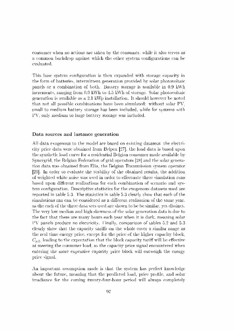
consumer when no actions are taken by the consumer, while it also serves asa common backdrop against which the other system con�gurations can beevaluated.

This base system con�guration is then expanded with storage capacity inthe form of batteries, intermittent generation provided by solar photovoltaicpanels or a combination of both. Battery storage is available in 0.9 kWhincrements, ranging from 0.9 kWh to 4.5 kWh of storage. Solar photovoltaicgeneration is available as a 2.1 kWp installation. It should however be notedthat not all possible combinations have been simulated: without solar PV,small to medium battery storage has been included, while for systems withPV, only medium to large battery storage was included.

Data sources and instance generation

All data exogenous to the model are based on existing datasets: the electri-city price data were obtained from Belpex [27], the load data is based uponthe synthetic load curve for a residential Belgian consumer made available bySynergrid, the Belgian Federation of grid operators [28] and the solar genera-tion data was obtained from Elia, the Belgian Transmission system operator[29]. In order to evaluate the stability of the obtained results, the additionof weighted white noise was used in order to e�ectuate three simulation runsbased upon di�erent realizations for each combination of scenario and sys-tem con�guration. Descriptive statistics for the exogenous datasets used arereported in table 5.3. The statistics in table 5.3 clearly show that each of thesimulations ran can be considered as a di�erent realisation of the same year,as the each of the three data sets used are shown to be be similar, yet distinct.The very low median and high skewness of the solar generation data is due tothe fact that there are many hours each year when it is dark, meaning solarPV panels produce no electricity. Finally, comparison of tables 5.2 and 5.3clearly show that the capacity tari�s on the whole cover a similar range asthe real time energy price, except for the price of the higher capacity block,Cp,2, leading to the expectation that the block capacity tari� will be e�ectiveat steering the consumer load, as the capacity price signal encountered whenentering the more expensive capacity price block will outweigh the energyprice signal.

An important assumption made is that the system has perfect knowledgeabout the future, meaning that the predicted load, price pro�le, and solarirradiance for the coming twenty-four-hour period will always completely

97

Descriptive Load data Solar Generation data Real time price datastatistics (kW ) (kW/kWp) (e/kWh)

Mean 0.41 0.41 0.41 0.22 0.23 0.23 0.08 0.08 0.08Median 0.40 0.40 0.40 0.00 0.00 0.00 0.09 0.09 0.09Skewness 0.56 0.56 0.57 1.82 1.82 1.83 -.077 -0.74 -0.96(unitless)Standard 0.14 0.14 0.14 0.37 0.37 0.37 0.04 0.04 0.04deviationMinimum 0.14 0.13 0.15 0.00 0.00 0.00 -0.38 -0.41 -0.43Maximum 1.02 0.94 0.94 1.98 1.97 1.84 0.32 0.31 0.32

Table 5.3: Descriptive statsitics of the exogenous data sets

match the corresponding realisations of that period. While this may besomewhat unrealistic, as in reality, some measure of forecast error will al-ways be present, this assumption was made in order not to only simplify themodeling work, but more importantly also to ensure that any forecast errorwould not skew or interfere with the research question at hand.

5.5 Results and discussion

First, the quantities of electricity bought from and sold to the grid are dis-cussed. Next, the yearly costs are analysed.

Figure 5.2 shows the amount of electricity bought from or sold to the elec-tricity grid, for the second week of January, under scenario A (no additionalpolicy intervention). This �gure mainly serves as a baseline for comparisonwith the policy intervention scenario B and C. It should also be noted thatthe results for the base case and the system with only 1.8 kWh of storage areidentical for scenario A, meaning they are superimposed over one another in�gure 5.2. Only one week's worth of simulated data is shown because suchan interval allows for the data to be displayed in a clear and legible way,while still showing the general trend that is present in all the data points.Similarly, the choice was made to only depict 4 system con�gurations outof the 8 investigated. Similar �gures for the four system con�gurations notshown here, can be found in appendix I. Additionally, the �gures appendedin appendix II present the same data as shown by the �gures discussed here,but grouped by system con�guration as opposed to by scenario. At this point

98

Figure 5.2: Second week of January for scenario A (�xed energy pricing, �xedcapacity pricing)

99

Figure 5.3: Second week of January for scenario B (�xed energy pricing,block capacity pricing)

also bears repeating that the resolution of the simulation is one data pointper hour, with the assumption that the energy quantities -so the load, char-ging or discharging storage and generation from solar PV- remain constantduring this one-hour window. This also means that the energy quantities de-picted in the �gures discussed in this section, are also the power �ows duringthat same hour: a load of 1 kW over the period of one hour corresponds to1 kWh and vice-versa.

Figures 5.3 and 5.4 show the system con�gurations during the second weekof January again, but now under policy scenario B and C respectively. As isimmediately apparent, the outcomes for both the base case and the PV sys-tem without battery storage do not change. This is as expected, as neither ofthose systems have battery storage, they cannot adapt their behaviour basedon the pricing scheme that is in e�ect. In contrast, the two systems depictedthat incorporate battery storage show marked changes. When comparing �g-ures 2 and 3, both depicted system con�gurations incorporating storage have�attened their respective peaks in �gure 5.3. This is expected behaviour, asboth simulated systems use their available storage components to avoid going

100

Figure 5.4: Second week of January for scenario C (spot energy pricing, blockcapacity pricing)

101

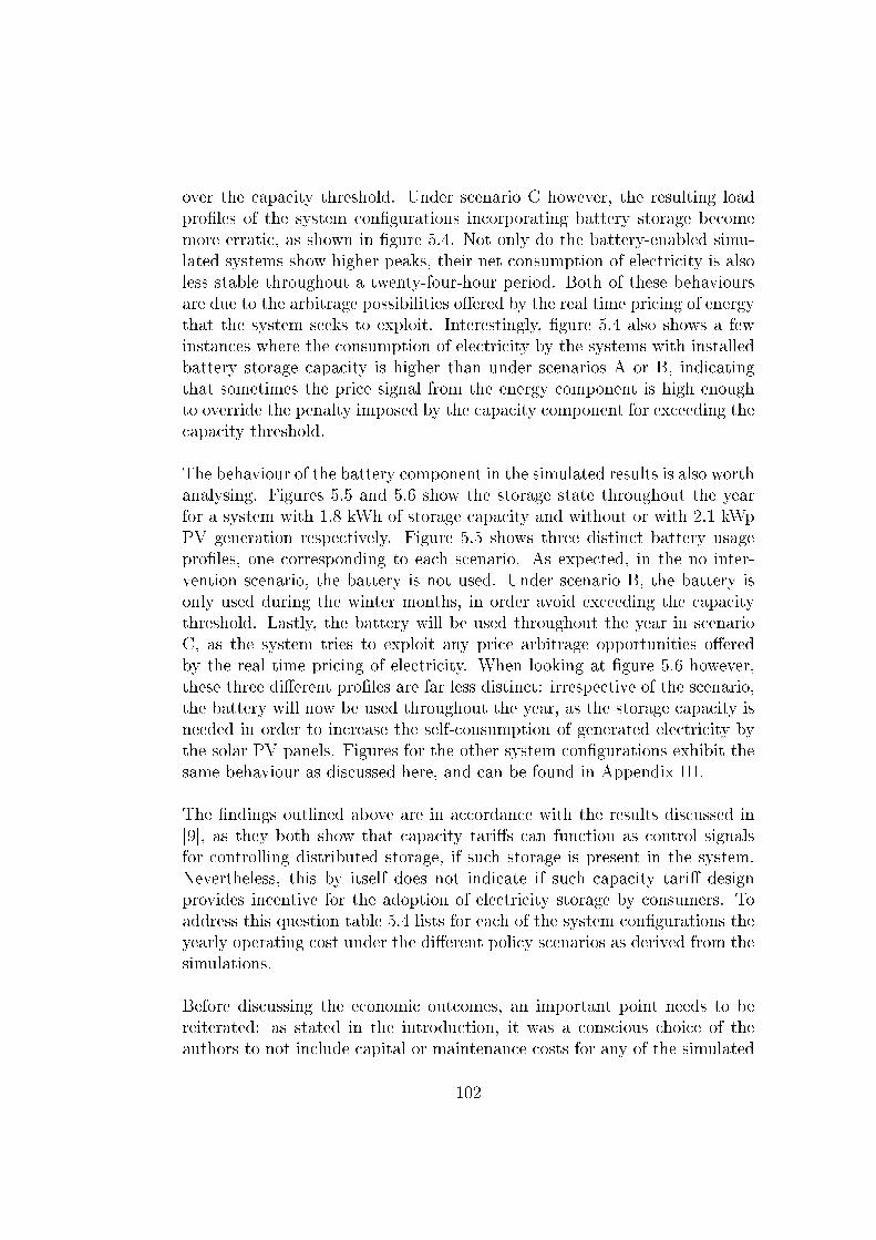
over the capacity threshold. Under scenario C however, the resulting loadpro�les of the system con�gurations incorporating battery storage becomemore erratic, as shown in �gure 5.4. Not only do the battery-enabled simu-lated systems show higher peaks, their net consumption of electricity is alsoless stable throughout a twenty-four-hour period. Both of these behavioursare due to the arbitrage possibilities o�ered by the real time pricing of energythat the system seeks to exploit. Interestingly, �gure 5.4 also shows a fewinstances where the consumption of electricity by the systems with installedbattery storage capacity is higher than under scenarios A or B, indicatingthat sometimes the price signal from the energy component is high enoughto override the penalty imposed by the capacity component for exceeding thecapacity threshold.

The behaviour of the battery component in the simulated results is also worthanalysing. Figures 5.5 and 5.6 show the storage state throughout the yearfor a system with 1.8 kWh of storage capacity and without or with 2.1 kWpPV generation respectively. Figure 5.5 shows three distinct battery usagepro�les, one corresponding to each scenario. As expected, in the no inter-vention scenario, the battery is not used. Under scenario B, the battery isonly used during the winter months, in order avoid exceeding the capacitythreshold. Lastly, the battery will be used throughout the year in scenarioC, as the system tries to exploit any price arbitrage opportunities o�eredby the real time pricing of electricity. When looking at �gure 5.6 however,these three di�erent pro�les are far less distinct: irrespective of the scenario,the battery will now be used throughout the year, as the storage capacity isneeded in order to increase the self-consumption of generated electricity bythe solar PV panels. Figures for the other system con�gurations exhibit thesame behaviour as discussed here, and can be found in Appendix III.

The �ndings outlined above are in accordance with the results discussed in[9], as they both show that capacity tari�s can function as control signalsfor controlling distributed storage, if such storage is present in the system.Nevertheless, this by itself does not indicate if such capacity tari� designprovides incentive for the adoption of electricity storage by consumers. Toaddress this question table 5.4 lists for each of the system con�gurations theyearly operating cost under the di�erent policy scenarios as derived from thesimulations.

Before discussing the economic outcomes, an important point needs to bereiterated: as stated in the introduction, it was a conscious choice of theauthors to not include capital or maintenance costs for any of the simulated

102

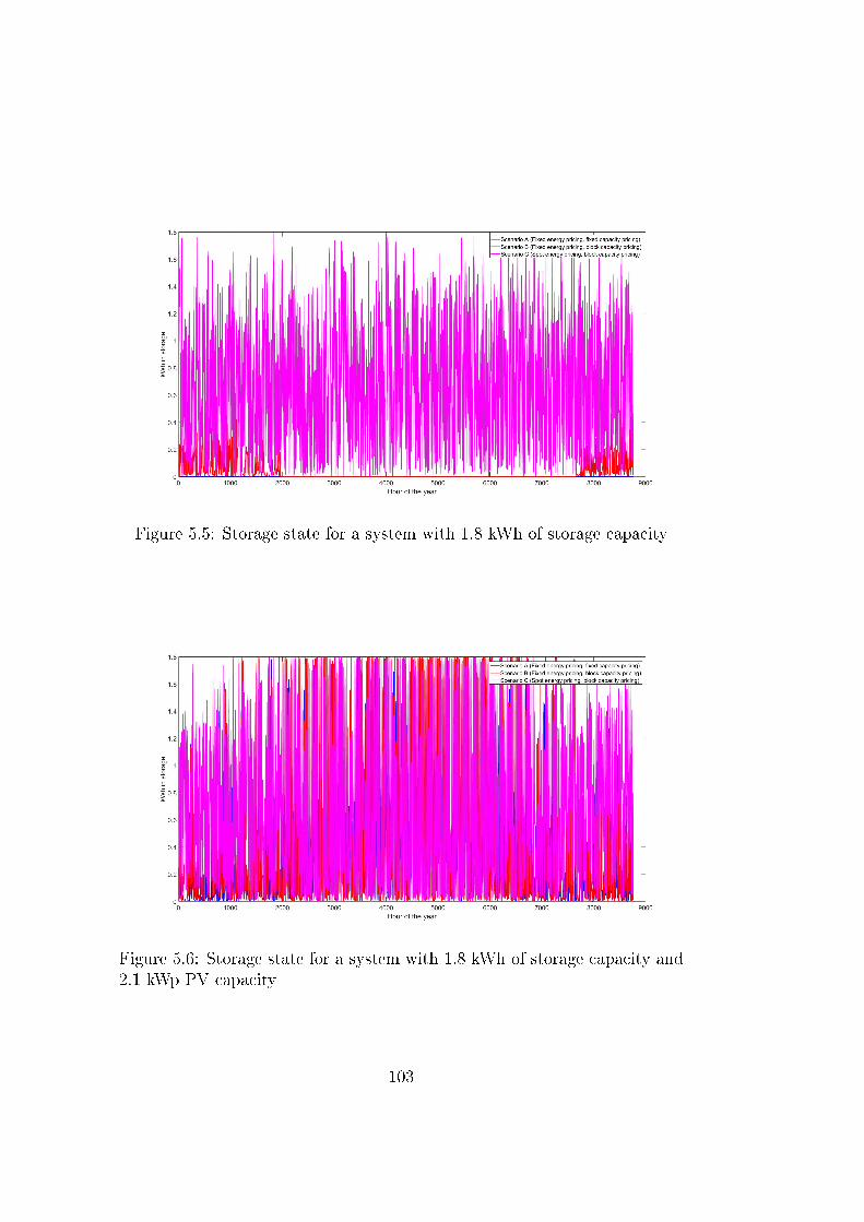
Figure 5.5: Storage state for a system with 1.8 kWh of storage capacity

Figure 5.6: Storage state for a system with 1.8 kWh of storage capacity and2.1 kWp PV capacity

103

System Con�guration Scenario

A B C

Base case 539.26 (0.37) 515.82 (1.31) 534.85 (1.20)0.9 kWh storage 539.26 (0.37) 539.59 (0.47) 547.00 (0.41)1.8 kWh storage 539.26 (0.37) 539.76 (0.55) 538.35 (1.33)3.6 kWh storage 539.26 (0.37) 540.38 (0.70) 534.39 (2.35)2.1 lkWp PV 272.90 (0.30) 401.75 (8.45) 419.17 (9.07)

1.8 kWh storage, 2.1 kWp PV 230.24 (0.72) 332.27 (6.15) 342.65 (7.16)3.6 kWh storage, 2.1 kWp PV 213.26 (0.24) 272.45 (4.88) 281.77 (5.19)4.5 kWh storage, 2.1 kWp PV 211.10 (1.06) 253.13 (4.50) 263.32 (5.28)

Table 5.4: Simulation results: average yearly operating cost in e (standarddeviation in e/year)

components. This has a signi�cant impact on how the results presented be-low should be interpreted: if there is a di�erence in reported costs betweenvarious rows in table 5.4, this does not immediately mean that the con�gura-tion with the lower reported cost is more economical and should be adopted,but rather provides a guideline by providing insight in the height of the annu-alised capital and installation cost which will allow the considered technologyto be economically viable. The bene�t of this approach is that it does not pinthe obtained results down to any speci�c level of technological advancementand technical performance but provides valuable insights valid regardless ofthe technical performance of the considered components.

Comparing columns A and B in table 5.4, it is clear that the block pricingcapacity tari� scheme does not have a large impact on the base case systemcon�guration. While this might seem counterintuitive, as this system con-�guration has no battery storage, meaning that it is impossible to shift anypart of the load to avoid exceeding Cb, for the majority of the observations,the used capacity remains below the capacity threshold. As denoted in table2, the capacity tari� for the lower block, Cp,1 is lower than Cp,f , so the ma-jority of the capacity used will be charged at a lower tari� under scenario Bas compared to scenario A, explaining the lower cost reported in table 5.4.When the combination of real time energy pricing and capacity block pricingis considered in scenario C, the results show that the outcome for the basecase scenario is a reduction of the yearly energy procurement cost.

Note that under scenario A, the resulting outcomes for the base case as wellas all the systems incorporating only battery storage are identical: the bat-

104

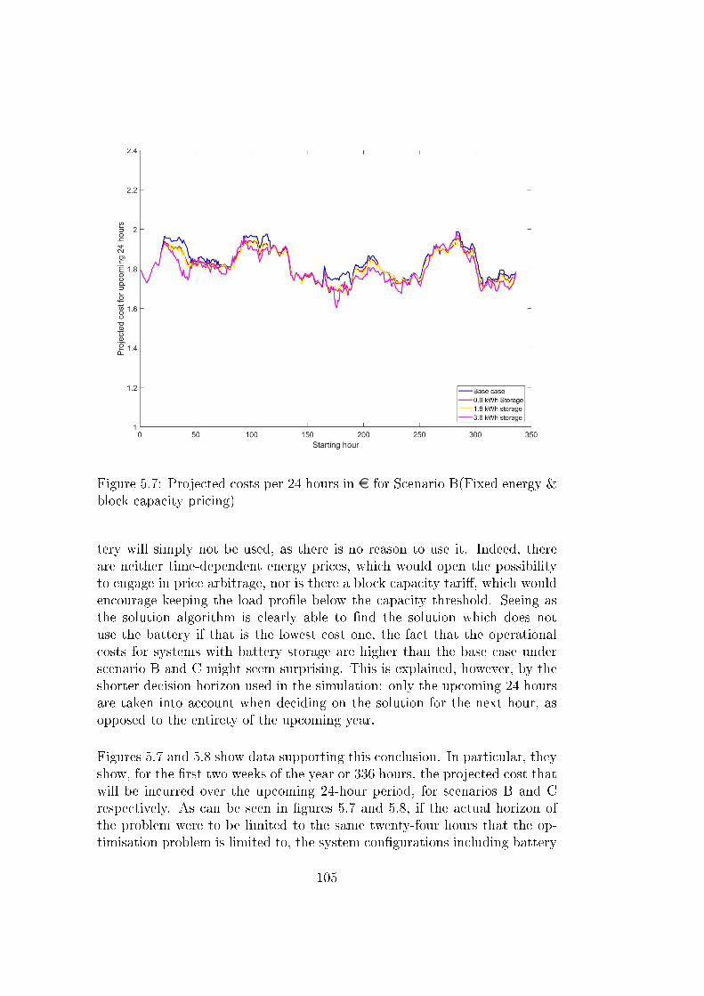
Figure 5.7: Projected costs per 24 hours in e for Scenario B(Fixed energy &block capacity pricing)

tery will simply not be used, as there is no reason to use it. Indeed, thereare neither time-dependent energy prices, which would open the possibilityto engage in price arbitrage, nor is there a block capacity tari�, which wouldencourage keeping the load pro�le below the capacity threshold. Seeing asthe solution algorithm is clearly able to �nd the solution which does notuse the battery if that is the lowest cost one, the fact that the operationalcosts for systems with battery storage are higher than the base case underscenario B and C might seem surprising. This is explained, however, by theshorter decision horizon used in the simulation: only the upcoming 24 hoursare taken into account when deciding on the solution for the next hour, asopposed to the entirety of the upcoming year.

Figures 5.7 and 5.8 show data supporting this conclusion. In particular, theyshow, for the �rst two weeks of the year or 336 hours, the projected cost thatwill be incurred over the upcoming 24-hour period, for scenarios B and Crespectively. As can be seen in �gures 5.7 and 5.8, if the actual horizon ofthe problem were to be limited to the same twenty-four hours that the op-timisation problem is limited to, the system con�gurations including battery

105

Figure 5.8: Projected costs per 24 hours in e for Scenario C(Spot energy &block capacity pricing)

106

storage would outperform the base case, with performance increasing withbattery size. While scenario C does allow the system con�gurations withbattery storage to engage in price arbitrage, resulting in lower costs thanunder scenario B, the price paid in optimization outcome due to the limitedhorizon is still the dominating factor, as even the largest of the simulatedstorage capacities is still outperformed by the base case system con�guration.

Probably the most interesting result, however, concerns the case of the solarinstallation without any storage capability. If there is no policy intervention,opting for the installation of solar PV without battery storage is by far themost cost-e�ective investment the simulated homeowner could make: yearlyenergy procurements are halved in this case, and no battery storage needsto be installed. However, as soon as block capacity pricing is introduced,the cost savings realized by the solar PV only system con�guration dropdramatically: the surplus of electricity produced by the solar PV systemshas to be sold to the grid, incurring hefty capacity charges. Where the basecase system con�guration saw a decrease in costs under real time pricingcombined with block capacity prices, a similar reduction in yearly costs doesnot hold true for the pure PV system, as for this system con�guration, theyearly energy procurement costs are highest when both policy interventionsare combined, as the peak production of solar PV does not coincide with themoments of peak electricity pricing.

The combination of PV generation and battery storage becomes much moreattractive when the battery storage is considered as an upgrade to an ex-isting PV system, as both under scenarios B and C, signi�cant savings aremade by transitioning from a pure PV system to a PV system with batterystorage. Speci�cally, in the case of the 3.6 kWh & PV and the 4.5 kWh &PV system con�gurations, adding that amount of battery storage allows thesimulated home owner to return to a pre-policy intervention yearly operatingcost, albeit with higher total system costs.

Seeing as this research is the �rst, to the best of the authors knowledge, toinvestigate the impact of capacity tari�s on the economics of microgrids, nodirect comparisons with earlier published research can be made. However,some parallels can still be drawn: �rstly, it is worth reiterating that, followingpublished �ndings in [9], capacity tari�s are able to steer consumer loads.Secondly, when comparing the proposed capacity tari� put forward in thisresearch with the time of use-schemes [18, 23], our results are in line with thepublished �ndings, in that the capacity tari� put forward does not encouragethe uptake of renewables. Furthermore, as table 5.4 shows, the proposed

107

capacity tari� actually disincentives the installation of solar PV: the yearlyoperating costs for a system with PV generation rises with nearly e130 ifblock capacity tari�s are implemented. However, this is not a problem whenthe stated goal of implementing the block capacity tari� is kept in mind,as it is aimed at promoting the uptake of storage systems, not necessarilyrenewables. Finally, our results are also in line with the �ndings publishedin [30], as the implementation of block capacity pricing, both separate fromas well as in conjunction with real time energy pricing does not negativelyimpact consumers who do not have any microgrid technologies.In summary, the results presented in this section show that the hypothesisput forward in section 5.3 holds: �gures 5.2,5.3 & 5.4 as well as �gures 5.5& 5.6 show the response, respectively of the system as a whole or of thebattery component, to the implementation of a block capacity tari�, andtable 5.4 clearly shows that the proposed block capacity tari� has virtuallyno impact on some system con�gurations, like the base case con�guration,or the battery only con�guration, while at the same time severely impactinga system con�guration that only has solar PV installed.Based on the above discussion, the policy implications are clear: if the policygoal is only to incentivise the adoption of storage in conjunction with, or asan upgrade to existing solar PV installations, implementing block capacitypricing should su�ce. In contrast, should it be the aim of policy makers toarrive at the widest possible adoption of storage, both capacity block pricingand real time electricity pricing will be useful, but will not su�ce by them-selves to provide a pro�table business case for grid-connected battery storage.

5.6 Conclusion

The impact of electricity tari� design on the adoption of battery storageis investigated. Using an optimization simulation model, the e�ect of twopolicy interventions is studied: (i) block capacity pricing and (ii) the com-bination of block capacity pricing and real time energy pricing on a variety ofsystem con�gurations, consisting of battery storage, solar PV generation ora combination of both. Due to the uncertainty and volatility of present andfuture prices for both battery storage and solar PV panels, the impact of theconsidered policy alternatives were investigated by comparing the simulatedaverage yearly operating costs of the di�erent system con�gurations to a basecase system con�guration without storage or solar PV. Notwithstanding thatcapacity tari�s have been shown to be e�ective at controlling the use of dis-tributed storage, our results show that these capacity tari�s by themselves

108

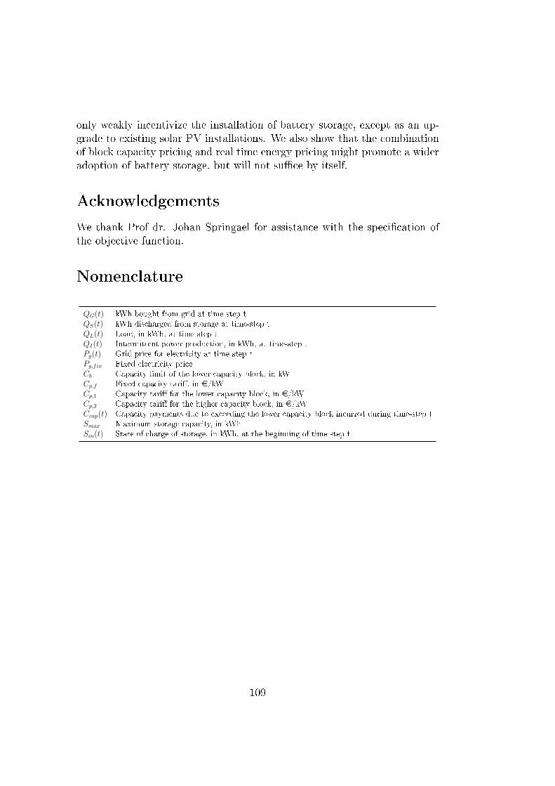
only weakly incentivize the installation of battery storage, except as an up-grade to existing solar PV installations. We also show that the combinationof block capacity pricing and real time energy pricing might promote a wideradoption of battery storage, but will not su�ce by itself.

Acknowledgements

We thank Prof dr. Johan Springael for assistance with the speci�cation ofthe objective function.

Nomenclature

QG(t) kWh bought from grid at time-step tQS(t) kWh discharged from storage at time-step tQL(t) Load, in kWh, at time step tQI(t) Intermittent power production, in kWh, at time-step tPg(t) Grid price for electricity at time-step tPg,fix Fixed electricity priceCb Capacity limit of the lower capacity block, in kWCp,f Fixed capacity tari�, in e/kWCp,1 Capacity tari� for the lower capacity block, in e/kWCp,2 Capacity tari� for the higher capacity block, in e/kWCcap(t) Capacity payments due to exceeding the lower capacity block incurred during time-step tSmax Maximum storage capacity, in kWhSin(t) State of charge of storage, in kWh, at the beginning of time step t

109

110

Bibliography

[1] Allan G, Eromenko I, Gilmartin M, Kockar I, McGregor P., The eco-nomics of distributed energy generation: A literature review, Renew andSustain Energy Rev, 2014 December; 40;269-86.

[2] Ringler P, Keles D, Fichtner W., Agent-based modelling and simulationof smart electricity grids and markets � A literature review, Renew andSustain Energy Rev, 2016 May;57;205-15

[3] Connor PM, Baker PE, Xenias D, Balta-Ozkan N, Axon CJ, CipciganL. Policy and regulation for smart grids in the United Kingdom, Renewand Sustain Energy Rev, 2014 December;40;269-86.

[4] Lasseter R, Akhil A, Marnay C, Stevens J, Dagle J, Guttromson R,et al., Integration of Distributed Energy Resources: The CERTS Mi-crogrid Concept. White paper. Prepared for the U.S. Department ofEnergy;2002

[5] Lidula NW, Rajapakse AD, Microgrids research: A review of experi-mental microgrids and test systems. Renew and Sustain Energy Rev,2014 August;36;428-39.

[6] IEEE Smartgrid [Internet], IEEE joint task force on quadrennial en-ergy review, Utility and Other Energy Company Business Case IssuesRelated to Microgrids and Distributed Generation (DG), EspeciallyRooftop Photovoltaics, Presentation to the U.S. Department of Energy2014, on the www, url:https://smartgrid.ieee.org/images/files/pdf/IEEE\_QER\_Microgrids\\\_October\_3\_2014.pdf

[7] Lo Prete C, Hobbs BF, Norman CS, Cano-Andrade S, Fuentes A, vonSpakovsky MR, et al., Sustainability and reliability assessment of mi-crogrids in a regional electricity market, Energy 2010 May;41;192-202.

[8] Palizban O, Kauhaniemi K, Guerrero JM. Microgrids in active networkmanagement-Part I: Hierarchical control, energy storage, virtual power

111

plants, and market participation, Renew and Sustain Energy Rev, 2014August;36;428-39.

[9] Hirsh A., Parag Y., Guerrero J. Microgrids: A review of technologies,key drivers, and outstanding issues, Renew and Sustain Energy Rev,2018 July;90;402-11.

[10] Yolda³ Y., Önen A., Muyeen S.M., Vasilakos A.V., Alan Ä°. Enhancingsmart grid with microgrids: Challenges and opportunities, Renew andSustain Energy Rev, May 2017;72;205-14.

[11] Milis K., Peremans H., Van Passel S. The impact of policy on microgrideconomics: A review, Renew and Sustain Energy Rev, January 2018;81-2;3111-119.

[12] Schreiber, M, Wainstein, ME, Hochlo�, P, Dargaville, R, Flexible elec-tricity tari�s: Power and energy price signals designed for a smartergrid, Energy 2015 December;93;2568-2581.

[13] Gouch, R, Dickerson, C, Rowley, P, Walsh, C, Vehicle-to-grid feasibility:A techno-economic analysis of EV-based energy storage, Applied Energy2017 April;192;12-23.

[14] Za�rakis, D, Chalvatzis, KJ, Baiocchi, G, Daskalakis, G, The value ofarbitrage for energy storage: Evidence from European electricity mar-kets, Applied Energy 2016 December;184;971-986.

[15] Aneke M, Wang M, Energy storage technologies and real life applications� A state of the art review, Applied Energy 2016 October;197;350-377.

[16] Martin-Martines F, Sánchez-Miralles A, Rivier M. A literature reviewof microgrids: a functional layer based classi�cation. Renew SustainEnergy Rev 2016 September;62;1133-53

[17] Siddiqui A, Marnay C, Edwards JL, Firestone R, Ghosh S, Stadler M.E�ects of a Carbon Tax on Microgrid Combined Heat and Power Adop-tion. J of Energy Eng 2005 April;131;2-25.

[18] Rocha P, Siddiqui A, Stadler M. Improving energy e�ciency via smartbuilding energy management systems: a comparison with policy meas-ures. Energy and Build 2105 February;88;203-13.

112

[19] Anastasiadis AG, Vokas G, Papageorgas P, Kondylis G, Kasmas S. Ef-fects of carbon Taxation, Distributed Generation and Electricity StorageTechnologies on a Microgrid. Energy Procedia 2014;50; 824-31.

[20] Mehleri ED, Sarimveis H, Markatos NC, Papageorgiou LG. Optimaldesign and operation of distributed energy systems: Application to greekresidential sector. Renew Energy 2013 March;51;331-42.

[21] Yu N, Kang J-S, Chang C-C, Lee T-L, Lee D-Y. Robust economicoptimization and environmental policy analysis for microgrid plan-ning: An application to Taichung Industrial Park, Taiwan. Energy 2016October;113;671-682.

[22] Zachar, M, Trifkovic M, Daoutidis P. Policy e�ects on microgrid eco-nomics, technology selection, and environmental impact. Comput andChem Eng 2015 October;81;364-75.

[23] Aghaei J, Alizadeh MI, Multi-objective self-scheduling of CHP (com-bined heat and power)-based microgrids considering demand responseprograms and ESSs (energy storage systems). Energy 2013 June;55;1044-54.

[24] Wang H, Fang H, Yu X, Liang S. How real time pricing modi�esChinese households� electricity consumption, J of Clean Prod 2018March;178;776-90.

[25] Kühnlenz F, Nardelli P, Karhinen S, Svento R. Implementing �ex-ible demand: Real-time price vs. market integration. Energy 2018April;149;550-65.

[26] Milis K, Peremans H, (2016): Economical Optimization of Microgrids:A Non-Causal Model. ASME. Energy Sustainability, Volume 2: Photo-voltaics; Renewable-Non-Renewable Hybrid Power System; Smart Grid,Micro-Grid Concepts; Energy Storage; Solar Chemistry; Solar Heat-ing and Cooling; Sustainable Cities and Communities, Transportation;Symposium on Integrated/Sustainable Building Equipment and Sys-tems; Thermo�uid Analysis of Energy Systems Including Exergy andThermoeconomics; Wind Energy Systems and Technologies.

[27] Historical market data [Internet] Epexspot Belgium, [cited 16 October2016], available from url:https://www.belpex.be/market-results/historical-data/

113

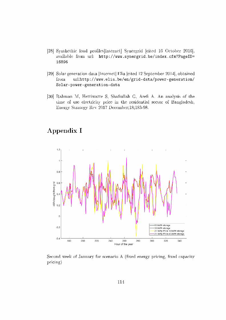
[28] Synthethic load pro�les[Internet] Synergrid [cited 16 October 2016],available from url: http://www.synergrid.be/index.cfm?PageID=

16896

[29] Solar generation data [Internet] Elia [cited 12 September 2014], obtainedfrom url:http://www.elia.be/en/grid-data/power-generation/Solar-power-generation-data

[30] Rahman M, Hettiwatte S, Sha�ullah G, Are� A. An analysis of thetime of use electricity price in the residential sector of Bangladesh,Energy Strategy Rev 2017 December;18;183-98.

Appendix I

Second week of January for scenario A (�xed energy pricing, �xed capacitypricing)

114

Second week of January for scenario B(�xed energy pricing, block capacitypricing)

115

Second week of January for scenario C (spot energy pricing, block capacitypricing

116

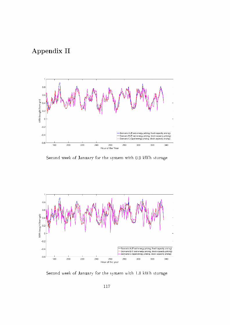
Appendix II

Second week of January for the system with 0.9 kWh storage

Second week of January for the system with 1.8 kWh storage

117

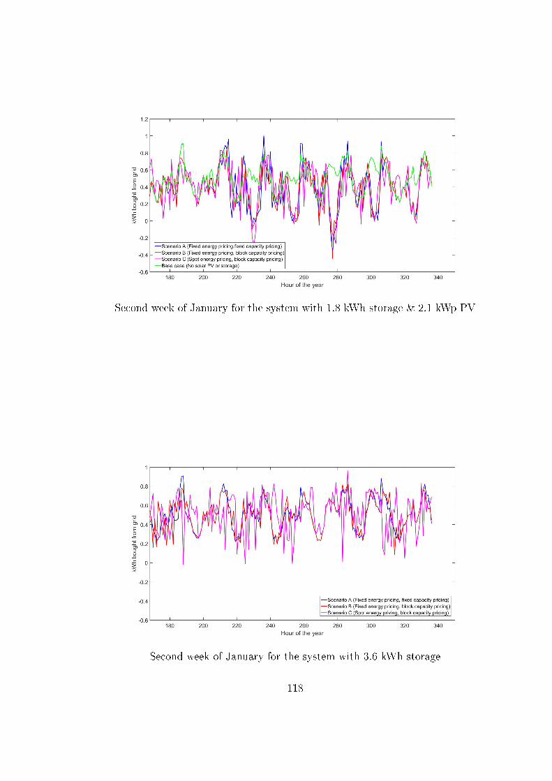
Second week of January for the system with 1.8 kWh storage & 2.1 kWp PV

Second week of January for the system with 3.6 kWh storage

118

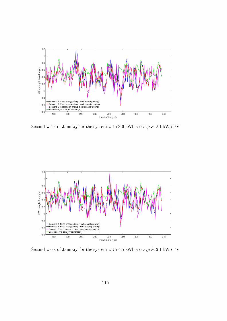
Second week of January for the system with 3.6 kWh storage & 2.1 kWp PV

Second week of January for the system with 4.5 kWh storage & 2.1 kWp PV

119

Appendix III

Storage state for a system with 0.9 kWh of storage capacity

Storage state for a system with 3.6 kWh of storage capacity

120

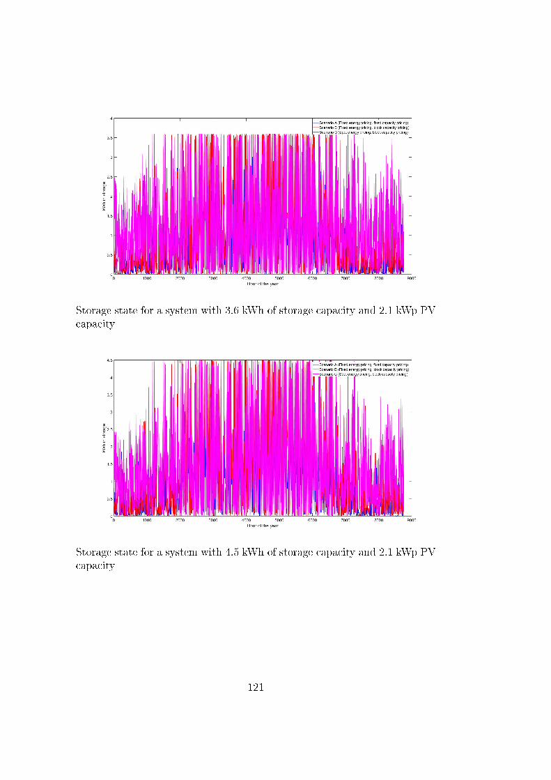
Storage state for a system with 3.6 kWh of storage capacity and 2.1 kWp PVcapacity

Storage state for a system with 4.5 kWh of storage capacity and 2.1 kWp PVcapacity

121

122

Chapter 6

Conclusion

6.1 Addressing the research question

This dissertation addressed the research question what is the economic valueof storage for a residential microgrid owner currently, and in case it provesto be negative, what are policy levers that can be used to adress this?, bylooking at three more speci�c research questions.

The �rst speci�c research question, what is the current economic value of stor-age for a residential microgrid owner?, is conclusively answered in chaptertwo. This chapter shows the unanimous result in the reviewed literaturethat electricity storage is not included in an economically optimal microgridcon�guration without some kind of governmental support, clearly showingthat the private economic value of storage is low. While the calculation ofthe exact societal bene�ts associated with storage are outside of the scopeof the work presented in the previous chapters, a clear case has been madein chapter 1 outlining the societal bene�ts o�ered by a greater penetrationof storage. However, the breadth of investigated policy measures is narrow,as the reviewed research focusses almost exclusively on feed-in tari�s on theone hand and investment incentives on the other hand. This is especiallysomewhat surprising given the fact research focussing on the utility side ofthe electrical grid has reported favourable outcomes with the use of capacitytari�s.

The second research question, What is a robust and insightful method tomodel microgrids, which allows for the investigation of di�erent policy in-terventions?, is addressed in several chapters. Chapter two shows that acombination of simulation modeling and optimisation is a widely excepted

123

practice in the �eld. The third chapter then explores the nature of the mod-eling problem at hand, while also showing that storage only really adds valueto a microgrid if either the reliability of the main in grid is low, or if thereare price arbitrage opportunity that can be exploited. The �rst of thosetwo possibilities is rather unlikely for a grid-connected microgrid in the de-veloped world, and the second possibility constitutes a policy intervention inan of itself. Chapter four, �nally, presents a further developed version of themodel presented in the third chapter, and shows that the proposed heuristicmethod is e�ective, thereby providing an answer to the methodologically in-clined sub-research question.

Chapter four's conclusions then also start to address the �nal research ques-tion, Which policy levers favour the installation of storage in residential mi-crogrids?, as they show that real time pricing of electricity, �meaning thatthe price of electricity is di�erent for each hour, as a function of supply anddemand� on its own, while making electricity storage attractive due to open-ing arbitrage opportunities, will lead to high capacity usage and a constanthigh load on the electrical grid. If real time pricing is however combined with�xed or block capacity pricing, the heavy peak usage of the electrical networkis mitigated. This is easily explained by the presence of capacity pricing: un-der �xed pricing, the grid connected parties will pay a �xed fee for each kWof grid capacity they use, either by injection into or withdrawal from the grid,while under a system of capacity block pricing, a �xed amount of capacity canbe used at a predetermined low tari�, and all capacity above this thresholdwill need to be remunerated at a higher tari�. While capacity block pricingresults in only slightly higher operational costs than �xed capacity pricing,the results demonstrate that capacity block pricing has the added bene�t ofreducing the amount of charge/discharge cycles the microgrid's battery ex-periences per day, thereby lengthening the expected lifetime of said battery.This combination of both public bene�ts, as evidenced by lower demandpeaks, which in turn allows for capacity reinforcement investment deferral,and private bene�ts, in the form of a longer battery lifespan, while at thesame time promoting the adoption of battery storage by microgrid owners,means that the combination of block capacity pricing with real time energypricing is a very promising policy measure in order to promote the uptake ofresidential battery storage.

The combination of real time energy pricing and block capacity pricing asanswer to the research question is further reinforced by chapter 5, as it notonly echoes the �ndings of chapter 4, but shows additional evidence why theproposed policy intervention would be robust: it would have no detrimental

124

e�ect on consumers without storage or solar panels, as most of the capacityusage is in the lower capacity price block, and peak household demand doesn'tcoincide with electricity price peak, the cost for a household without any mi-crogrid technologies will even see a slight reduction in yearly operating costs.This is a non-trivial result from a social point of few, as the case can be madethat poorer households will lack the �nancial means to invest in microgridtechnologies, and would therefore be obliged to accept the consequences ofany policy intervention on the base case system con�guration, without anypossibility to adopt new technologies. System con�gurations with batteriesalso see an improvement in their yearly operational costs, and it are only thesystem con�gurations with PV that are negatively a�ected, however, thise�ect can largely be mitigated by installing battery storage which allows formore of the produced electricity to be self-consumed, instead of being injectedinto the grid and incurring high capacity charges at times of peak production.

6.2 Key messages beyond the research question

In addition to the answers formulated in response to the research questionabove, there are also other important conclusions put forward by this workthat bear repeating here.

Firstly, the literature review conducted in chapter two has revealed that alack of e�ort is oft-times put into reporting the speci�cs of the simulationor case that was studied, omitting information about installed generationcapacity, or overall load served. This makes it almost impossible to replicatethe results presented, which hampers the advancement of knowledge in the�eld.

Secondly, chapter four shows that interesting and promising results can beobtained by adopting an innovative approach to the accepted methodology.Additionally, the work put forward in chapter four shows that the adop-ted methodology not only impacts the overall obtained results, but can alsodirectly impact the behaviour of the modeled components, reinforcing themessage that it is important to make a well-considered choice when pickinga methodological approach.

125

6.3 Limitations

A number limitations are worth mentioning, the �rst two of which are bothrelated to the assumed exogeneity of the timeseries in the model. The �rst ofthese is the consumer load. A case can be made that it would interesting tomodel the consumer load as endogenous to the model, meaning that the con-sumer load shifts in response to the current electricity prices charged on themarket. Modelling this would however require signi�cant amounts of extradata: in order to model this in any insightful way, the consumer's load pro�lewould need to be split in up in separate load pro�les for each appliance, afterwhich separate demand price-elasticities would need to be estimated corres-ponding to these appliances. It is worth pointing out, however, that theexplicit inclusion of storage allows to largely sidestep this problem: storageprovides a bu�er which, size permitting, decouples the actual load pro�le ofthe consumer from the demand pro�le that the grid experiences. In this way,storage actually allows for automated demand response, without the needfor consumer interaction. One extra insight the behavioural approach coulddeliver would be the convenience value of storage provided by this automa-tion, as opposed to manually having to monitor grid prices and adjustingbehaviour.

Along a similar vein, the price of electricity is also assumed to be exogenousto the simulation model. This is a reasonalbe assumption when the size ofthe simulated system is taken into account: the simulated microgrid is alwayssmall compared to the main grid, meaning that the microgrid operates as aprice taker, with no means to a�ect the equilibrium price. It would howevercertainly be interesting to let go of this assumption and look at microgridsthat are large enough to signi�cantly impact the market they connect to.This idea will be touched upon as well in the next section, as a possible av-enue of further research.

It is important to note that the focus of this work is exclusively on theprivate, economics bene�ts of storage, only tangentially touching upon thepublic bene�ts of storage, which can be both economic in nature, such asallowing for capacity investment deferral, or societal, such as allowing for theincreased penetration of local, intermittent generation, of which the economicvaluation is less clear cut. Integrating data on these latter two values wouldenhance the analyses conducted, as it would allow for a discussion on thepercentage of the positive externalities that needed to be internalised beforestorage becomes economically viable at the level of a private actor, onlyconsidering his private bene�ts.

126

6.4 Future outlook

While the research question put forward has been conclusively answered bythe work presented, interesting other avenues of research can be formulated.

A �rst one concerns capacity tari� design itself: the tari� design used through-out this body of work has been proven to be e�ective, but that does notpreclude the existence of better designs, such as for instance a tari� withmore than two parts, or one with a more pronounced di�erence between thetwo (or more) tari� levels. Closely linked to di�erent designs of capacitytari�s is the balance between the energy component on the one hand, andthe capacity component on the other hand: these are the two parts of theobjective function that drive the operational cost that the microgrid will besubjected to, and they drive microgrid behaviour in opposite directions. Thecapacity component favour microgrid behaviour that uses as little capacityas possible, while the energy component promotes heavy usage of the gridthrough price arbitrage. Based on this reasoning, an investigation focussingon the balance between the two might yield interesting results.

A second promising avenue of research is expanding the work presentedwithin to multiple interconnected microgrids. This is an interesting prob-lem, as it fundamentally changes the behaviour of the modelled system: inthe case of the grid-connected microgrid discussed in this booklet, the size,both in terms of generation and load of the microgrid has always been smallcompared to the main grid, meaning that the microgrid could only acceptedthe market conditions on the main grid, without being able to in�uence them.In a scenario of multiple interconnected microgrids, this is no longer the case,as now the actions of a single microgrid can signi�cantly impact the stateof the entire network. This also means that the energy and capacity tari�design used needs to be able to communicate information about this stateof the network between all connected parties, since balancing the network isnow a shared responsibility amongst all interconnected actors.

127