Forschungsinstitut zur Zukunft der ArbeitInstitute for the Study of Labor

DI

SC

US

SI

ON

P

AP

ER

S

ER

IE

S

Economic Activity and the Spread of Viral Diseases:Evidence from High Frequency Data

IZA DP No. 9326

September 2015

Jérôme Adda

Economic Activity and the Spread of Viral Diseases:

Evidence from High Frequency Data

Jérôme Adda Bocconi University, IGIER and IZA

Discussion Paper No. 9326 September 2015

IZA

P.O. Box 7240 53072 Bonn

Germany

Phone: +49-228-3894-0 Fax: +49-228-3894-180

E-mail: iza@iza.org

Any opinions expressed here are those of the author(s) and not those of IZA. Research published in this series may include views on policy, but the institute itself takes no institutional policy positions. The IZA research network is committed to the IZA Guiding Principles of Research Integrity. The Institute for the Study of Labor (IZA) in Bonn is a local and virtual international research center and a place of communication between science, politics and business. IZA is an independent nonprofit organization supported by Deutsche Post Foundation. The center is associated with the University of Bonn and offers a stimulating research environment through its international network, workshops and conferences, data service, project support, research visits and doctoral program. IZA engages in (i) original and internationally competitive research in all fields of labor economics, (ii) development of policy concepts, and (iii) dissemination of research results and concepts to the interested public. IZA Discussion Papers often represent preliminary work and are circulated to encourage discussion. Citation of such a paper should account for its provisional character. A revised version may be available directly from the author.

IZA Discussion Paper No. 9326 September 2015

ABSTRACT

Economic Activity and the Spread of Viral Diseases: Evidence from High Frequency Data*

Viruses are a major threat to human health, and - given that they spread through social interactions - represent a costly externality. This paper addresses three main issues: i) what are the unintended consequences of economic activity on the spread of infections? ii) how efficient are measures that limit interpersonal contacts? iii) how do we allocate our scarce resources to limit their spread? To answer these questions, we use novel high frequency data from France on the incidence of a number of viral diseases across space, for different age groups, over a period of a quarter of a century. We use quasi-experimental variation to evaluate the importance of policies reducing inter-personal contacts such as school closures or the closure of public transportation networks. While these policies significantly reduce disease prevalence, we find that they are not cost-effective. We find that expansions of transportation networks have significant health costs in increasing the spread of viruses and that propagation rates are pro-cyclically sensitive to economic conditions and increase with inter-regional trade. JEL Classification: I12, I15, I18, H51, C23 Keywords: health, epidemics, spatial diffusion, transportation networks, public policy Corresponding author: Jérôme Adda Department of Economics Università Bocconi Via Roentgen 1 20136 Milano Italy E-mail: jerome.adda@unibocconi.it

* I gratefully acknowledge coeditors Larry Katz and Andrei Shleifer, and three anonymous referees for many valuable comments and suggestions. I am grateful to Christian Dustmann, Jonathan Eaton, Andrea Ichino, Matt Neidell, Emily Oster and participants in seminars at the universities of Bergen, Brown, Darmstadt, Duke, Mannheim and Stockholm for helpful comments and discussion.

I. INTRODUCTION

Viruses are a major threat to human health. Over the last century, viruses were responsi-

ble for many more deaths than all armed conflicts that took place during that period. For

instance, smallpox killed about 300 millions individuals during the twentieth century. In-

fluenza was responsible for about 100 million deaths, a large part of them during the major

outbreak in 1918-1919, known as the Spanish flu, but also through more recent pandemics.

Other viruses also contribute to this sombre statistics, which include HIV (about 30 million

deaths so far) and a number of viruses leading to gastroenteritis (about one million deaths

per year worldwide).1 In modern societies, with individuals in better health, viruses are also

an important cause of morbidity and loss of productivity. For instance, in the US, about 30

million cases of gastro-enteritis are reported each year, leading to 120,000 hospitalizations.

Likewise, influenza results in about 200,000 hospitalisations per year. Viruses impose there-

fore a cost on society, through premature deaths, long-lasting morbidity (Almond (2006),

Kelly (2011)), increased health-care utilisation and loss of schooling or hours of work. More

broadly, as emphasised by Fogli and Veldkamp (2013), the prevalence of diseases can be

linked to social network structures and have long-term effects on growth.

In this paper, we provide a number of contributions to the understanding of the role

of social interaction and economic activity in the spread of viruses. First, we exploit data

that are unusually detailed, describing the incidence of three major viral diseases: influenza,

gastro-enteritis and chickenpox. The data spans a period of up to a quarter of a century,

at a weekly frequency, across geographical locations in France. Moreover, the data allow us

to distinguish between age groups, an important element, as children and the elderly are

particularly vulnerable populations, with potentially different transmission patterns. These

data allow us to analyse the spatial and temporal evolution of diseases in a developed econ-

omy. This focus is novel in the economics literature, which has mostly studied the incidence

of one particular virus, HIV, usually in developing countries (Oster (2005) or Oster (2012)).2

1For an overview of the determinants of mortality in developed and developing countries over time, see

Cutler et al. (2006).2The economic literature has been fruitful because the spread of HIV relies on the choice of individuals

whether to protect them-selves or not and part of the trade-off is through the beliefs of the prevalence of

2

Second, we use quasi-experimental variation to assess the effectiveness of various measures

such as closing down schools, shutting down public transportation or expanding railways on

the transmission of a number of viruses. Closing down schools during influenza epidemics is

routinely done in countries such as Japan or Bulgaria. In addition, a number of countries

such as China, France, the United Kingdom and the United States have used this measure

during the 2009 pandemic (Cauchemez et al. (2014)). Closing down temporarily public

transportations or declaring a general curfew is a more drastic measure to curb an epidemic.

There is a long history of quarantines to prevent the spread of diseases, which dates back

at least to the plague epidemics in Europe and Asia in the Middle Ages. It has been used

selectively during the Ebola outbreak in 2014, but not for seasonal epidemics.

The paper improves on the literature in epidemiology, which has developed models of

disease diffusions dating back to Kermack and McKendrick (1927). 3 The work in epidemi-

ology provides little direct and data based evidence on the effectiveness of policies aiming at

reducing population contact rates. When this is the case, this literature also ignores impor-

tant issues such as measurement errors, serial correlations and endogeneity, which are likely

to bias the results. We assess the role of transportation infrastructures in the propagation of

diseases in two ways. First, we exploit public transportation strikes throughout this period.

In France, this is a relatively common occurrence, with a variety of general and more local

strikes. Second, we exploit the extensive development of high speed railways across regions

of France, and we use openings of new lines to assess their effect on the speed of disease

transmissions. We further evaluate the role of peer-effects and spill-over effects by using

information on school closures due to holidays. School holidays vary within the year and

across the country, allowing for variability across time and space. Moreover, these closures

are decided well in advance and are therefore unrelated to the prevalence of diseases, which

helps to remediate reverse-causality issues.

the disease. Early such contributions focussing on “rational epidemics” include for instance Geoffard and

Philipson (1996) or Kremer (1996). Auld (2006), Lakdawalla et al. (2006) and Dupas (2011) investigate the

role of beliefs and prevalence on behavior, whereas Greenwood et al. (2013) look at equilibrium models of

disease transmission.3 Anderson and May (1991) provide an overview of this literature. New developments include Epstein

et al. (2007) or Lempel et al. (2009) that develops calibrated agent-based models.

3

A third contribution is to investigate the long-run economic determinants of the spread

of viruses. This is an under-explored area, which is important to better understand how

epidemics and economic activity are related. In the context of developed countries, and for

common viral diseases, there are many unanswered questions: do viruses propagate faster

during economic recessions or booms; does the unemployment rate contribute to epidemics;

what is the role of inter-regional trade in the transmission of diseases4; do viruses spread

symmetrically across space or do they follow a gradient determined by economic factors? To

answer these questions, we develop a dynamic and spatial model of diffusion, based on work

in epidemiology, which is estimated, paying particular attention to measurement error, serial

correlation and endogeneity, using instrumental variable techniques.

We find that school closures have a pronounced effect on the incidence of influenza,

reducing its incidence for a period of about three to four weeks. This effects is stronger

for children, but also sizable for adults. We find similar effects for gastro-enteritis and

chickenpox, although the effect is more short-lived and less important. Moreover, we find

that for the elderly, such measures can increase the incidence in the short-run. Our results

suggest therefore important spill-overs across age groups, within the extended family. We

find significant decreases in the transmission rates of diseases during public transportation

strikes, which mirrors the increased transmission rates following extensions of railway lines.

By exploiting data for three viral diseases, which differ in several aspects, such as incubation

time or infectiousness our results also shed light on how efficient those measures can be on

emerging diseases that share some of the same characteristics as the ones we consider.

We next calculate the expected monetary benefits of such measures, using cost estimates

from the literature. We find that although closing down schools for a period of 2 weeks

would reduce the total annual incidence of some of the diseases by up to 12 percent across

all age groups, such measures represent an overall cost to society. We find similar results,

although with smaller costs, for a policy that would close down public transportations for

a week. We show that those measures would become beneficial for epidemics characterised

by a slightly more deadly strain, or for a policy that would match the closure of schools

4Prior work exists on the link between trade and HIV infection as Oster (2012) shows that increased

exports in African countries lead to higher infection rates.

4

during epidemics with a longer term time in the summer. We also evaluate the health costs

of expanding transportation infrastructures. Connecting two regions with a high-speed rail

link generates a cost of about 80 million euros per year, through higher medical costs and

loss of productivity. This cost is of the same order of magnitude as the time saved by faster

transportation.

We find that epidemics spread faster during economic booms. During booms more people

are traveling which increase inter-personal contacts and the spread of diseases. This is in

contrast with the work in epidemiology that has found that diseases are more prevalent in

bad times, although this literature relies mostly on aggregate cross-country comparison us-

ing annual data (see for instance the meta-analysis by Suhrcke et al. (2011) and the papers

reviewed therein). Our results also add to the literature linking health and in particular

mortality to business cycles, which was pioneered by Ruhm (2000). This literature finds

that mortality declines during recessions and has been attributed to changes in health be-

haviour (Ruhm (2003), Ruhm (2005) and Evans and Moore (2012)). Our results point to

an additional channel, which mitigates the health behaviour channel, at least for mortality

due to infectious diseases or respiratory causes.

The rest of the paper is organized as follows. Section II. gives medical information on the

viruses we study, which are important to interpret the results in the next sections. It also

describes the various data set used in the analysis. Section III. presents an event analysis

describing the effect of school closures and transportation strikes. Section IV. presents a

dynamic and spatial model of viral spread, discusses econometric issues and presents the

results. Section V. investigates the cost efficiency of different policy measures. Section VI.

evaluates the health cost of transportation infrastructures. Finally section VII. concludes.

II. Viral Diseases: Data and Descriptive Statistics

In this section, we provide an overview of the characteristics of the viral diseases we study

as well as details on public health measures in France between 1984 and 2010, the period we

consider in the empirical section. We then present the data we analyse.

5

II.A. Disease Characteristics and Prophylactic Measures

We consider three major viral diseases, influenza, gastroenteritis and chickenpox. All diseases

are caused by specific viruses, and as such, cannot be treated by drugs such as antibiotics.

They usually result in infections that last for two to ten days. In some cases, infected

individuals can develop complications, that may result in death, especially for people with

health predispositions or for elderly individuals.

Table I provides a brief comparison of all three diseases, with information on incubation

time, approximate duration of symptoms and the period when an infected individual becomes

contagious. For influenza, the incubation period ranges from 2 to 5 days. Acute diarrhea

caused by viruses incubates in about a day. On the other hand, chickenpox takes much

longer to incubate, a period of between two to three weeks. For this particular disease,

infected individuals acquire a life-long immunity. This is not the case for influenza and

gastroenteritis, as the viruses involved mutate very quickly. While it is rare to get a second

bout of influenza in the same year, it is possible to contract gastroenteritis several times in

a year.

For each of these diseases, vaccines exist, but they vary in their efficacy and their use by

public health authorities. In the case of influenza, in France, as in many developed countries,

vaccination is targeted towards the elderly, health care workers and a small minority of people

at risk. The coverage was about 70 percent for the elderly, 16 percent for adults and only

6 percent for children in 2010. These number have risen over time, as the practice was

to provide immunization for people above 75 in 1985, and then above 65 from year 2000.

In the case of gastro-enteritis, vaccination is difficult as many viruses, such as rotaviruses,

noroviruses or adenoviruses, can be the cause of the disease. A first vaccine against the

rotavirus A was developed in 1999 but then withdrawn because of side-effects. A new vaccine

is on the market since 2006, but few countries have a systematic vaccination plan. French

public health authorities advised against the use of the vaccine in 2010 and recommended

instead a better use of re-hydration therapies in grave cases. For chickenpox, a vaccine was

developed in 1988. It is widely used in the US, but not in Europe, where it is considered

potentially more dangerous than the disease itself. As a consequence, immunity is acquired

6

almost entirely through exposure to disease when children are in day care or in primary

school.

The average yearly incidence (percentage of population that get infected in a given year)

differs widely across diseases. Table I presents typical ranges for the US and European

countries. Gastroenteritis is the most prevalent disease, with an incidence rate varying

between 20 and 40 percent. The incidence of influenza varies widely as well, depending on

the viral strain that is present, ranging from 5 to 20 percent in the case of seasonal influenza.

In pandemic years, the figure can be much higher for both gastro-enteritis and influenza. The

1918 pandemic infected about 30% of the population (Taubenberger and Morens (2006)).

The incidence of chickenpox is much lower in the total population for two reasons. It is

almost exclusively a childhood disease and countries differ in the use of vaccines. In the UK

or France where no vaccination occurs, the incidence corresponds roughly to the number

of babies born each year, as eventually almost all of them will get contaminated by the

chickenpox virus. In the US, due to vaccination, the prevalence is only about 0.1%.

II.B. High Frequency Data on Disease Prevalence

We use detailed, high frequency (weekly) data on disease incidence in France, covering a

period of up to 25 years. The data is available for three age groups - children (aged 0-

18), adults (18 to 64) and the elderly - and at regional level.5 The data is unique in the

sense that no other countries have tried to gather systematic measures of incidence over

such a long period and for several viral diseases. For instance, the data on influenza for

the US, collected by the CDC, cover only the period from 1997 onwards, and for broad

regions. Similarly, Google6 reports data on flu epidemics, but only from 2003. Although

their estimations track public health data quite well on average, it is unclear how to break it

down by smaller geographical regions, and even more by age groups. There is also an issue

with trends in internet usage, across region or age groups that could lead to measurement

error. For other viral diseases, such as gastroenteritis or chickenpox, the data is even more

5Mainland France is subdivided into 21 regions. The average population size of a region was 2.1 million

in 2009, ranging from 0.7 million (Limousin, around Limoge) to over 6 million (Paris).6See http://www.google.org/flutrends/.

7

scarce.

The data we use on disease incidence come from the ”Reseau Sentinelles”, a network of

about 1,300 general practitioners which was set-up in 1984 as a public health surveillance

system by the Institut de Veille Sanitaire (InVS).7 Those physicians report each week the

number of cases of many diseases diagnosed on the basis of the symptoms and medical exam-

ination of the patient. However, their assessment is not based on the analysis of biosamples,

which would ascertain the viral origin of the disease. Hence, to be precise, the data pertain

to influenza-like illnesses rather than influenza and acute diarrhea rather than gastroenteritis

and we shall label them as such in the reminder of the paper. The data is aggregated up to

regional level, before its release.

Figure I displays the time series patterns of incidence rates at the national level and on a

weekly basis between 1984 and 2010. Flu-like illnesses, acute diarrhea as well as chickenpox

have recurrent peaks each year during the winter season. Given the seasonal fluctuations, it

is difficult to see whether the incidence of these diseases has increased or decreased over this

period. Table II displays the average annual percentage increase in the incidence of all three

diseases, by age groups.8 The situation is contrasted. The incidence of flu-like illnesses is

stable for children, but has decreased for both adults and the elderly, by about two to five

percent per year. One reason for this downward trend is the increased uptake of vaccination,

especially for older individuals. In contrast, the incidence of acute diarrhea has increased by

one to two percent per year over the period 1990-2010, and for all age groups. The incidence

of chickenpox for children has not changed in a significant way during that period.

Figure II displays the average incidence rate within a year, by calendar week, from the

first week of January to the last week of December. The graph distinguishes the incidence

rate by age groups. The incidence rate is inversely related to age. Some diseases such as

chickenpox are almost exclusively a childhood disease, while influenza and acute diarrhea

can also affect older individuals. As seen in the previous graphs, flu-like illnesses and acute

diarrhea show strong seasonal patterns with a peak in winter and a low incidence between

mid-spring to mid-fall. Chickenpox has a different pattern across the year. The incidence is

7The Reseau Sentinelles represents about 1-2 percent of all general practitioners in France over the period

we analyze and cover the whole of France. Appendix A provides further details about the network.8The results are obtained from regressing the log average annual incidence per 100,000 on a linear trend.

8

roughly constant up to July, then decreases substantially during the summer and increases

thereafter. The decrease coincides with the summer vacations of French schools. We return

to the influence of school closure on epidemics below in more detail.

One reason for the higher incidence of viral diseases in recent times (at least among

the non-vaccinated population) as shown in Table II can be due to the fact that diseases

tend to propagate faster than before. Over time, improvement in public transportation

and communication infrastructures, increases in trade across regions may help to spread

diseases faster. This is important as a fast-evolving epidemic is more difficult to contain.

We investigate this point in Table III, where we test whether yearly epidemics reach a peak

earlier in the year in more recent times. It is sometimes difficult to identify a unique peak in

the incidence rate, as in some regions or years, there could be several of them. We therefore

define the seasonal peak as the date when the cumulative infection rate reaches 80% of

the total infection rate. This often coincides graphically with the maximum incidence. We

experimented with different cut-offs and got very similar results. Given the seasonality of

these diseases, we start the year in the first week of July, when infection rates are generally

at their lowest. We calculate the time to the peak (expressed in weeks since July) for each

region r, each year t and each age group g and denote this variable TTPrgt. This resulted in

1,573 durations (combination of year, region and age groups) for flu-like illnesses and 1,259

durations for acute diarrhea, as the data start only in 1990. We do not attempt the analysis

for chickenpox, given that its seasonal pattern is not as marked. We regress the duration to

reach this threshold on a constant, a trend (expressed in years), indicator variables for each

age group and region indicators:

TTPrgt = a0 + a1yeart + a2AgeGroupg + a3Regionr + urgt (1)

Table III displays the results. For each additional year, the time to reach the peak decreases

by 0.07 weeks for flu-like illnesses and 0.4 weeks for acute diarrhea. In other words, the

results indicate a faster spread of these diseases over the period of observation. Note also

that the peak is reached first for children and last for the elderly, with a difference of about

a week.

9

II.C. Potential Determinants of the Spread of Diseases

We give details on the data used to explore the determinants of the spread of diseases. We

refer the reader to appendix A for additional information on data on weather and population

density.

1. School Closures. In France, schools close for vacation five times a year. The summer

break lasts for about eight weeks, usually from the beginning of July to the beginning of

September. The other vacation breaks last between one and two weeks and take place around

October-November (All Saints break), the end of December (Christmas break), February-

March (winter break) and April-May (spring break). The calendar is set by the Ministry

of Education about two years in advance, and is binding for all public and private schools.

Some breaks apply to all regions at the same time, mostly for the autumn, Christmas and

summer breaks. For the winter and spring holidays, France is divided into two or three zones,

depending on the year, and these zones have a staggered break. Some regions have school

holidays earlier than others, with a difference that can reach four weeks. For the epidemics

we study, a period of four weeks is large as they evolve quickly. Moreover, some regions have

shifted from one zone to another. Hence, with up to 25 years of data, there is variability

across years and across regions in school closures, which we exploit to infer the causal effect

of school closures on the spread of diseases. This variability allows us to control for region

fixed effect and for week fixed effects, as vacation periods have additional variation.

We obtained data from the Ministry of Education on all school holidays for all regions

between 1984 and 2010. The school holidays often coincide with vacation taken by parents,

especially at Christmas, and often during the winter break. French workers are entitled to

5 weeks of vacations, since 1981. From the year 2000, adults also obtained more vacation

as the hours worked per week were capped at 35 hours on average during the year. A large

number of workers stayed on a 39 hour week schedule, but were then entitled to 25 additional

days of vacation, leading to a total of 8 weeks of vacations. This implies that parents can

often take vacations at the same time as their children. Hence, the effect of school holidays

on epidemics has to be interpreted in this broader sense.

10

2. Public Transportation Strikes. We focus on strikes affecting the French national railways

(SNCF) which lasted more than three days in a row. In France, railways are an important

mean of transportation, as governments have massively invested in railway after the Second

World War, when railway lines were targeted by bombings. As a result, French passengers

travel on average 1,370km per year by rail, which puts France in the top three countries for

rail travel in the world, and the first one in Europe. In the case of a railway strike, travelers

can switch to road transportation, but given the limited capacity of roads and highways,

these become rapidly blocked, which limits transportation further. Hence a railway strike

seriously limits population movements within and across regions.

We searched the popular press through the LexisNexis interface between the year 1984 to

2010 for all strike events that lasted more than three days. Most of the strikes are national,

but there are some instances of regional strikes in particular in the south-east of the country.

Train strikes often occur when unions and the government negotiate over employment or

pay. We recorded between 19 and 28 weeks of strike, depending on the region, between 1984

and 2010, roughly one week of strike per year. Figure IIIa plots the frequency of these strikes

during the calendar year and by duration. Strikes occur most often between October and

May, with no strikes during the summer. Hence, railway strikes are more likely to occur

during the influenza and gastroenteritis epidemic seasons. To eliminate this confounding

effect, we control in all the regressions below for week (and year) effects and we assume that

the date of the strike is exogenous once we control for such variables. Strikes last on average

for about a week and a half, with half of the strikes lasting less than 8 days (see Figure IIIb).

3. High Speed Railway Openings. Since the seventies, the French government has developed

a network of high speed trains, which travel at speeds up to 200 miles per hour. We use

precise data on the date of openings of high speed rail lines. The first line opened on

September 27, 1981 and connected Paris to Lyon, the second largest city in France. Since

that date, the network expanded throughout France, linking major cities, with the latest

addition in 2007, between Paris and Strasbourg in the east of France. Figure IV plots the

main high speed rail-lines in France together with the date they opened. These lines became

major transportation routes, as they cut transportation time substantially. For instance a

11

typical journey from Paris to Marseille on the French riviera was cut from about 7 hours to

only 3 hours. The number of passengers travelling on these trains grew from 1.26 million in

1981 to almost 100 million in 2010. Between 1981 and 2013, 2 billion passengers travelled

on the high speed train network.9

At first, the lines were connecting Paris to major cities. However traveling between two

cities other than Paris remained complicated as one had to connect in Paris, where different

train stations were handling trains to and from the south, the north or the west. The

connection time could add a couple of hours to a journey as well as the hassle of transferring

luggage through the Parisian public transportation system. Gradually, major cities became

linked without the need of transfer as trains avoided the connection in the centre of Paris.

We also use these openings in our empirical model (although the dates do not appear on

Figure IV to avoid cluttering). We include a series of indicator variables which take the

value of one from the moment two regions become connected by a high-speed train without

a connection in Paris. In our empirical model, these networks are only affecting the inter-

regional transmission of diseases, as the lines have few, if any, stops within a region.

4. Economic Activity. One aim of this analysis is to evaluate how economic activity influ-

ences the rate of transmission of viral diseases. There are several potential indicators of

economic activity, which have been used in previous work, which include income (see Et-

tner (1996), Adams et al. (2003) or Adda et al. (2009)), per capita GDP, unemployment

rates (Ruhm (2000) and the literature that enfolded), or trade and exports in a context

of HIV infections (Oster (2012)). Although these indicators all capture some aspect of the

business cycle, they are also specific to certain aspects of health that the previous literature

has focused on. Changes in income may affect use of health care or health behavior such

as alcohol consumption or smoking. Unemployment may affect more particularly mental

health. We follow the empirical literature on infectious diseases and opt for inter-regional

trade as our main measure of economic activity. Higher trade may be associated with higher

rates of traveling within and across regions, determining the rate of interpersonal contacts.

The choice is also due to lack of data on income at regional level for the earlier part of our

9The development of high-speed trains reduced the share of travellers by plane and cars along those

routes, but also attracted many new travellers.

12

sample. Nonetheless, trade is highly correlated with aggregate GDP (correlation=0.92) and

track expansions and recessions well. We also explore the role of unemployment and how

it may affect propagation rates. Further details on the trade data we use can be found in

appendix A.

III. School and Public Transportation Closures:

Evidence from an Event Analysis

We start by analyzing the dynamics of the incidence of the diseases within regions, following

two particular events: school closures due to holidays and strikes that shutdown the public

transportation system. Analyzing the global effect of these events within and across regions

requires further modeling. This is also the case with other determinants that do not have

as sharp temporal variation as the two variables we study. We defer such modeling to

Section IV. and start with an event analysis, where an event is defined as the first week of

school closure or of a public transportation strike. Denote the incidence of a disease in region

r, and week t by Irt and by Ert an indicator variable equal to one if schools are closed or

public transportations are on strike in that period. We also define as Trt the average weekly

temperature. We estimate the following equation by OLS, for each disease and age group:

Irt =K∑

k=−3bkEErt−k + bTTrt + bXXrt + vrt (2)

The matrix Xrt includes a constant, region fixed effects, week of the year fixed effects and

year effects. We cluster the standard errors by region.

The coefficients bkE are displayed in Figures V and VI. For ease of interpretation, we

normalise these coefficients by b−1E to display the relative incidence of the disease compared

to the one in the week prior to the event. In the case of school closures, we find a sharp

decline in the incidence of flu-like illnesses, of a magnitude between 20 to 30 percent. This

decrease is sustained for at least 4 weeks. The effect is more pronounced for children than for

adults or the elderly, but still statistically significant between the weeks 3 to 5 for the latter.

For acute diarrhea, the effect of school closure is less pronounced (a decreace in incidence of

about 10 percent) and more short-lived. The effect disappears after the third week. Finally,

13

for chickenpox, we find a statistically significant effect for children after 4 weeks, with a

reduction of about 10 percent in the incidence. Figure VI displays similar statistics in the

case of a public transportation strike. For flu-like illnesses, the effect is sustained for about 2

weeks for children and adults. We do not find statistically significant effects for the elderly,

nor for the other diseases (acute diarrhea and chickenpox).

In summary, the event analysis suggests a marked effect of school closures and public

transportation strikes on the dynamics of diseases, and for various age groups. It is interesting

to see that school closures have an effect not only on children, but also on adults and even

the elderly. This suggests sizable interaction effects between various age groups.

IV. Model of Viral Spread Within and Across

Regions

We now develop a dynamic model of the spread of viral diseases, within and across regions,

which is based on models of infections developed in the epidemiology literature. This model

is suited to analyse the complex interactions between several determinants of the spread of

diseases, both over time and across space. We then discuss its empirical implementation as

well as important identification issues.

IV.A. Standard Inflammatory Response Model

The medical literature on infectious diseases has modeled epidemics using a Standard Inflam-

matory Response (SIR) model. This model is able to describe the dynamics of an epidemic

in a concise but accurate way (Kermack and McKendrick (1927), Anderson and May (1991)).

Let S denote the fraction of individuals who are susceptible to contract the disease, I the

fraction of individuals who are infected and R the fraction of individuals who have recovered

but are still immune. At any point in time, the equality S + I +R = 1 holds. The model is

14

usually expressed in continuous time and the flows into each category are expressed as:

dIdt = αSI − βIdRdt = βI − λRdSdt = −αSI + λR

(3)

The first equation in (3) describes how the number of infected individuals evolves over a

short interval of time. A fraction β of those infected recover from the disease, while new

cases develop, at a rate α. β−1 is the average infectious period. New infections occurs from

the interaction of susceptible and infected individuals, hence the multiplicative formulation.

The stock of recovered individuals is increased by the number of individuals who exit the

infectious state and is decreased by the fraction of individuals who lose their immunity, at a

rate λ. The stock of susceptible individuals is increased in each period by the flow of recovered

individuals who lose their acquired immunity. At the same time the stock is decreased by the

fraction of individuals who become infected. The rate λ varies considerably across the various

viral diseases we consider. For chickenpox, λ is equal to zero, as individuals acquire a life-

time immunity. Hence, within a birth cohort, the stock of susceptible individuals decreases

towards zero as they age. In contrast, individuals who had a spell of gastro-enteritis have

almost no immunity, and λ is expected to be high. The case of influenza is an intermediate

one. We return to this issue in the empirical section, where we explain how we construct a

measure of the stock of susceptible individuals.

The dynamics of the epidemic depends on the ratio α/β, the basic reproduction number.

If this ratio is greater than one, an epidemic develops, whereby the fraction of infected

individuals sharply increases in a very short time-span. The epidemic eventually dies out as

the population of susceptible individuals approaches zero or as the proportion of infectious

individuals vanish. The model describes the propagation of viruses within a closed society.

In reality, there are also individuals who are sick coming from other regions, so the fraction

of infected individuals also depends on the fraction of infected individuals in other regions

or countries. The model can be extended such that the number of new cases is equal to

αwithinSI+αbetweenSI, where I is the fraction of infected individuals from outside the region

of interest who meet susceptible people from within the region.

For influenza, typical parameter values are β = 1/2.6 days and α/β = 1.8 (Ferguson

15

et al. (2006)). Public health interventions are unlikely to change β, which is a biological

parameter. Its value depends on the type of virus and the particular strain, but there

is usually no treatment that shortens the infectious period. On the contrary, it is likely

that the transmission rate, α, varies across space and time. Its value can also be changed

by suitable interventions as the transmission rate depends on the frequency of contacts

between infectious and susceptible individuals. Hence, the model predicts that keeping sick

individuals at home, closing schools or workplaces will lower, at least temporarily, the spread

of an epidemic.

The parameter α is also a behavioral parameter as sick individuals decide whether or not

to mix with susceptible individuals (and vice-versa). The economic literature on rational

epidemics (see Kremer (1996), Geoffard and Philipson (1996), Philipson (2000) or Chan

et al. (2015)) has extended the epidemiological models to take into account how individuals

react to changes in prevalence. However, in the case of many viral diseases, contaminated

individuals become infectious before the symptoms become apparent, which mitigate the

scope for avoidance. Moreover, as most viral diseases are benign, the cost of avoidance

can outweigh the benefits of avoidance of potentially infected individuals. The literature on

rational epidemics has therefore focused mostly on the case of sexually transmitted diseases

such as HIV. 10 Taking into account behavioral changes for the diseases we study is difficult

as it would require data on whether individuals protect them-selves by interacting less with

others, or whether they wash their hands more often during epidemics.11

The transmission parameter α will also depend on many factors such as population

density or the rate at which individuals travel. Hence, the spread of epidemics depends both

on long-run and short-run demographic and economic factors. In the long-run, the spread

of viruses depends on how a society is organized and how integrated the economy is, as

discussed in Fogli and Veldkamp (2013). Developing roads, highways, rail connections or

airports may increase the speed of propagation and the number of cases.

In the short-run, the strength of an epidemic may depend on fluctuations in economic

10Empirical evidence that individuals alter their behavior in response to the perceived risk they face include

Adda (2007), Thornton (2008), Neidell (2009), Moretti and Neidell (2011) and de Paula et al. (2013).11If behavioral adjustment is important, it would imply that the parameter α is decreasing with the per-

ception individuals have of the likelihood of contracting the disease. We test this conjecture in Appendix D.

16

activity, for at least two reasons. First in good times, more individuals may travel and meet

people for business purposes. Second, unemployed individuals may have different patterns

of socializing, which may lead to different propagation rates. Ruhm (2000) shows that

individuals are in better health during recessions. Part of the effect is due to changes in

health behavior, which leads to fewer deaths during recessions. Whether epidemics and viral

contagion fluctuates with the business cycle remains an open question we address in this

paper.

The literature in epidemiology has produced an important body of research to devise

public health strategies to curb viral epidemic, especially for influenza. 12 This work often

relies on calibrated parameters, which are chosen partly based on medical information (in-

fectious period) and partly on average durations and scope of an epidemic. With such an

approach, it is difficult to empirically evaluate the role of policies as one lacks sharp and

exogenous variation for identification. Another strand of the literature has estimated models

of diffusion using OLS, Bayesian or simulation techniques, using high frequency data. How-

ever, this literature has failed to consider the endogenous nature of important explanatory

variables.13

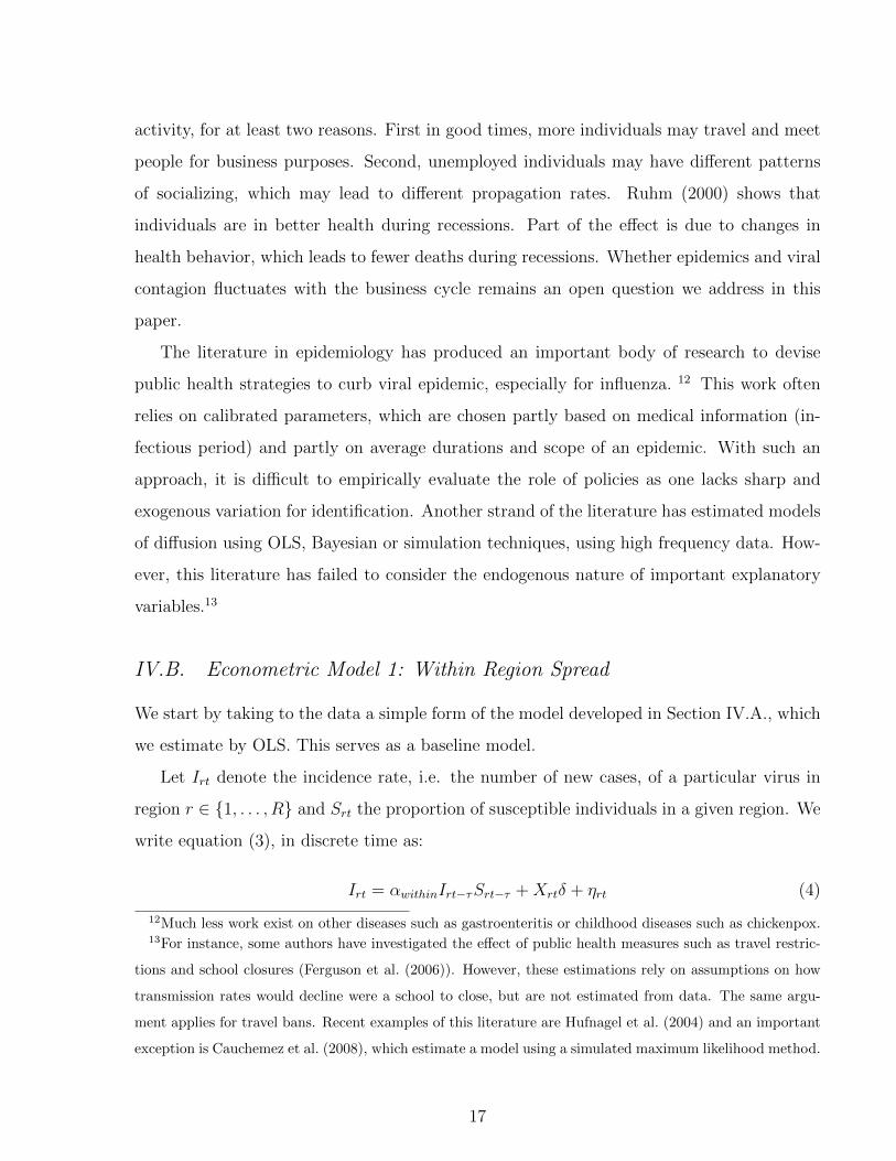
IV.B. Econometric Model 1: Within Region Spread

We start by taking to the data a simple form of the model developed in Section IV.A., which

we estimate by OLS. This serves as a baseline model.

Let Irt denote the incidence rate, i.e. the number of new cases, of a particular virus in

region r ∈ {1, . . . , R} and Srt the proportion of susceptible individuals in a given region. We

write equation (3), in discrete time as:

Irt = αwithinIrt−τSrt−τ +Xrtδ + ηrt (4)

12Much less work exist on other diseases such as gastroenteritis or childhood diseases such as chickenpox.13For instance, some authors have investigated the effect of public health measures such as travel restric-

tions and school closures (Ferguson et al. (2006)). However, these estimations rely on assumptions on how

transmission rates would decline were a school to close, but are not estimated from data. The same argu-

ment applies for travel bans. Recent examples of this literature are Hufnagel et al. (2004) and an important

exception is Cauchemez et al. (2008), which estimate a model using a simulated maximum likelihood method.

17

where the matrix Xrt includes region fixed effects, week effects and year effects in levels. The

parameter τ represents the incubation time. For acute diarrhea and flu-like illnesses, we set

τ to one week, as both diseases incubates in less than a week (see Table I). For chickenpox,

we set τ to 3 weeks.

We identify the model without relying solely on time variation or cross-section varia-

tion, which could confound many of the effects. The implementation using a difference-in-

difference identification strategy is also a departure from the existing literature in epidemiol-

ogy. The shock ηrt is possibly serially correlated, which would lead to bias since equation (4)

is essentially a lagged dependent model. We deal with this issue below. We use a panel-

corrected standard error procedure allowing for heteroskedasticity, spatial correlation across

regions and for serial correlation of the form of an autoregressive process of order one.

The estimation of equation (4) requires the computation of the stock of the susceptible

population, Srt for each region and year. We proceed in different ways for each viral disease,

taking into account the differences on how immunity is acquired.

For influenza, the chances to get a second bout in the same year is low (although not

zero). We assume that immunity lasts for a year, until a new epidemic starts. Given the

seasonality patterns of the disease, we define the start of the year to be at the beginning of

July, when the infection rate is at its lowest. The stock of susceptible individuals in a given

week is therefore the entire population minus those who are vaccinated and those who have

been infected previously since the end of the previous July.14

For gastro-enteritis, we assume that immunity only lasts for a week after the end of the

infection. Hence the stock of susceptible individuals consists of the entire population minus

the fraction who were ill the previous week. Given the low efficiency of the vaccine and its

rare usage in France (the vaccine was first produced in 2006), we do not consider it in the

computation of the susceptible population.

In the case of chickenpox, a contaminated individual acquires a life-time immunity. Hence

the susceptible population consists mostly of very young children. We construct the stock

14Data on vaccination rates per age groups were obtained from GEIG, a French public health institute

(see http://www.grippe-geig.com). The data is at the national level, but broken down by age groups and we

predict the incidence of vaccination in each region and year based on the age structure of the population.

18

of susceptible individuals for each period and region by combining data on the incidence of

diseases in the previous years, as well as data on the size of birth cohorts across region and

time. The exact procedure is detailed in Appendix B.

For ease of interpretation, we have normalised the susceptible population by the total

population in the region in a particular age group. Hence, the coefficients presented are to be

interpreted as marginal effects of a change in the infection rate on the future infection rate,

when the entire population is susceptible to the disease. However, as a disease progresses,

the pool of susceptible individuals decreases, which implies smaller marginal effects. The

results are displayed in Table IV, Panel A. Each column represents a separate regression

for different diseases or age groups. In the case of flu-like illnesses, each infected individual

infects 0.28 children, 0.46 adults and 0.1 elderly individual. In the case of acute diarrhea,

the estimates indicate that an infected individual transmit the disease to 0.18 children, 0.26

adults and 0.03 elderly individuals. Finally, a child infected with chickenpox spread it to

0.18 other children. These estimates are significant at the one percent level, but are on

the low side, as each infected individual is transmitting the disease to fewer than one other

individual in total. If that is indeed the case, then these diseases should not evolve into

epidemics, which is counterfactual. The reason for this discrepancy is that the estimation is

likely to be biased for several reasons, including measurement error and omitted variables.

IV.C. Econometric Model 2: Within and Between Region Spread

We next introduce a spatial dimension to the model, and we let the incidence rate of region

r be determined by the incidence rate of other regions as well. Given that the pattern of

socialisation across regions is likely to be different from the ones within a region, we allow

the transmission parameter α to be different within and between regions:

Irt = αwithinIrt−τSrt−τ + αbetween∑c∈R\r

Ict−τSrt−τ +Xrtδ + ηrt (5)

The set of all other regions includes all regions R minus region r, denoted R\r. In this

specification, each region has the same effect, regardless of distance or connection. We

introduce differential effects across region below.

19

1. OLS Results. We estimate model (5) by OLS and display the results in Table IV, Panel

B. Each individual infected with a flu-like illness is spreading the disease to 0.24 children,

0.41 adults and 0.1 elderly individuals within the same region. In addition, this individual

infects 0.005 children, 0.006 adults and 0.003 elderly individuals in each of the other regions.

Although the number of further infected individuals in the same region is lower than the one

found in Section IV.B., the total number of infected individuals is now slightly above one.15

The estimated propagation rates are also higher for acute diarrhea and chickenpox, but still

well below one in total. This points out that it is important to take into account spatial

diffusion across regions, but also that the estimates are still potentially biased.

2. Instrumental Variable Results. As argued above, there are several reason why OLS esti-

mates of equation (5) may be biased. First, the possible serial correlation in the error term

would lead to bias the OLS estimates, given the dynamic structure of the model. Second,

measurement error would also lead to bias. The data on the incidence of diseases are esti-

mated from the number of cases seen by a network of general practitioners, which is subject

to sampling error. Given that the incidence of diseases appears as an explanatory variable,

it is important to take this fact into account. We show in Appendix C that measurement

error leads to a complex error term, with serial dependence. Hence, equation (5) cannot be

consistently estimated by OLS.

To get consistent estimates of the transmission parameters, we use instrumental variables.

We have two variables to instrument, the within-region lagged incidence times susceptible

rates, Irt−τSrt−τ , and the one across regions,∑c∈R\r

Ict−τSrt−τ . We use lagged weather episodes

as instruments. There are biological reasons to consider those variables as instruments.

Viruses, especially influenza, do not survive well in warmer temperatures, but can cope well

with cold and dry conditions (e.g. Lowen et al. (2007)). Viruses responsible for gastro-

enteritis are also sensitive to warmer temperatures (Moe and Shirley (1982)). Moreover,

adverse weather may also influence socialising patterns and the rate at which viruses are

15The total number of infected individuals is obtained by summing the coefficients across age groups, and,

in the case of between region coefficients, by multiplying by the number of regions minus one. The analysis

uses 21 regions.

20

passed on from person to person. In the case of diseases with some degree of acquired

immunity (influenza or chickenpox), the number of susceptible individuals, Srt−τ , displays

inertia and previous weather episodes are particularly suited instruments. For the within

region term, we construct the number of weeks with temperatures below 0, 5, 10, . . . ,

25 degrees Celcius, from the end of the preceding summer (when incidence rates are at the

lowest). Similarly, we construct the amount of rain in the preceding four and eight weeks. We

therefore use a total of 8 instruments.16 For the between region term, we use 11 instruments,

consisting of the ones detailed above and three measures of the number of regions with weekly

temperatures below 0, 10 and 20 degrees Celsius. This aggregate measure of temperature

determines the sum of the incidences across all regions (except r).

As seen in Table I, each disease vary in terms of length of incubation and duration of

symptoms. Hence it is likely that the effect of weather is stronger at various lags, depending

on the disease we study. This is precisely what we find. We use a one week lag for acute

diarrhea and for flu-like illnesses and a three week lag for chickenpox. For the latter disease we

also use the size of the birth cohorts, at regional level, in the preceding six years. Indeed, as

those who contract the disease acquire near full immunity, the pool of susceptible individuals

consists mainly of young children and a larger birth cohort in a given year and a region

leads to a larger pool of susceptible individuals a few years laters, when this cohort enters

kindergarten or primary school. The regression also includes region, year and week fixed

effects. We test for the joint significance of the instruments and present the F-test and its

associated p-value in Table V.17 The instruments work well, with all the p-values well below

the 5 percent level. The table also displays R-squares, which vary between 0.3 and 0.8. Note

that our first stage is stronger for children and adults, compared to the elderly. It is also

stronger for the susceptible population interacted with the incidence rate in other regions,

which is equivalent to the national incidence rate minus the one in the region of interest.

The reason is that lagged weather is a better predictor of the national incidence rate than

the regional ones.

The results are displayed in Table IV, Panel C. Compared with the OLS results presented

16In the case of chickenpox, we also include the size of the birth cohort within the region in the last 6

years.17Table I in the appendix provides a full list of the first stage coefficients.

21

in Panel A and B of the same table, the transmission rates are globally larger. One individual

with flu-like illnesses spread the disease to about 1.27 individuals, within and across regions

and age groups. In the case of acute diarrhea and chickenpox, the number of infected

individuals is equal to 1.08 and 1.9 respectively.18 The Hausman test displayed at the

bottom of the table shows that exogeneity of the regressors is rejected in six out of seven

cases. The results in the last panel highlight the importance of taking into account the

endogenous nature of the dependent variables and of allowing for spatial effects.

3. Econometric Model 3: Full Model. We now consider a complete model, where the trans-

mission rate is time-varying and region specific. Allowing for heterogenous effects in the

coefficient of interest, α, in the context of a dynamic model, is rare in the economic litera-

ture, especially relying on differential variations across space and time. It is feasible, given

that we are relying on a small cross-section of regions and a large time span.

Denote a set of K region-specific variables W krt that potentially influence the transmission

rate of diseases within a region. They include those already mentioned earlier, such as school

closure and transportation strike indicators. We add to the model the effect of temperature,

heavy rainfall or snow, population density, a measure of economic activity (volumes of trade

within the region), quarterly dummies and a time trend. For the transmission rates across

regions, denote a set of K variables W krct, which measure characteristics specific to regions

r and c. For instance, the variable can be a binary indicator equal to one when schools

in both regions are closed, when both regions experience a train strike or when they are

linked by a high speed train connection. We add to those measures inter-regional trade,

distance between regions (defined as the distance between the most populous cities in each

region), population ratios, log regional GDP ratios and temperature differences. These latter

variables capture potential asymmetries in the spatial transmission of viruses. We also allow

for quarterly dummies and a time trend to affect the inter-regional spread. Although the

model includes many determinants of viral spread, some of them have of course been left

18The literature in epidemiology has produced numbers which are of similar magnitude, although slightly

higher. The basic reproduction number for influenza is usually around 2. The one for chickenpox is closer to

7, compared to the one found in the analysis of about 4, taking into account the fact that the disease lasts

for about 2 weeks.

22

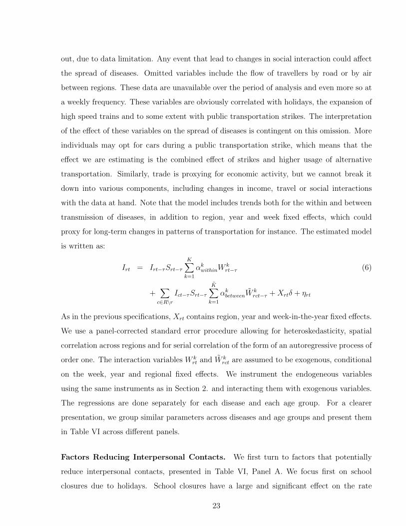
out, due to data limitation. Any event that lead to changes in social interaction could affect

the spread of diseases. Omitted variables include the flow of travellers by road or by air

between regions. These data are unavailable over the period of analysis and even more so at

a weekly frequency. These variables are obviously correlated with holidays, the expansion of

high speed trains and to some extent with public transportation strikes. The interpretation

of the effect of these variables on the spread of diseases is contingent on this omission. More

individuals may opt for cars during a public transportation strike, which means that the

effect we are estimating is the combined effect of strikes and higher usage of alternative

transportation. Similarly, trade is proxying for economic activity, but we cannot break it

down into various components, including changes in income, travel or social interactions

with the data at hand. Note that the model includes trends both for the within and between

transmission of diseases, in addition to region, year and week fixed effects, which could

proxy for long-term changes in patterns of transportation for instance. The estimated model

is written as:

Irt = Irt−τSrt−τK∑k=1

αkwithinWkrt−τ (6)

+∑c∈R\r

Ict−τSrt−τK∑k=1

αkbetweenWkrct−τ +Xrtδ + ηrt

As in the previous specifications, Xrt contains region, year and week-in-the-year fixed effects.

We use a panel-corrected standard error procedure allowing for heteroskedasticity, spatial

correlation across regions and for serial correlation of the form of an autoregressive process of

order one. The interaction variables W krt and W k

rct are assumed to be exogenous, conditional

on the week, year and regional fixed effects. We instrument the endogeneous variables

using the same instruments as in Section 2. and interacting them with exogenous variables.

The regressions are done separately for each disease and each age group. For a clearer

presentation, we group similar parameters across diseases and age groups and present them

in Table VI across different panels.

Factors Reducing Interpersonal Contacts. We first turn to factors that potentially

reduce interpersonal contacts, presented in Table VI, Panel A. We focus first on school

closures due to holidays. School closures have a large and significant effect on the rate

23

of transmission to children, with a decrease of 0.14 individuals infected in the case of flu-

like illnesses, 0.07 individuals for acute diarrhea and 0.19 individuals for chickenpox. The

effect is relatively strongest for flu-like illnesses and weakest for chickenpox, in line with the

results obtained with the event analysis in Section III. The incubation period for this disease

is longer than the usual school vacation, which ranges from one to two weeks, except for

summer holidays. School holidays also decrease the transmission rate of flu-like illnesses for

adults with a reduction of about 0.1 people infected. However, the effect for acute diarrhea

in adults is positive but not significant. The elderly are affected in different ways. There

is a small but insignificant decrease (at the 5% level) for flu-like illnesses, but a significant

increase in the propagation rate for acute diarrhea. In principle, the effect of school closure

could go in opposite directions. School closures may decrease the general incidence of a

disease and lead to an indirect effect on the elderly. On the other hand, school holidays are

also a period when children are more likely to interact with their grand-parents, and could

therefore be a period of heightened infectiousness. The overall effect is therefore ambiguous,

with a detrimental effect for acute diarrhea.

The second row of the panel displays the effect of school holidays on the transmission

across regions. As noted in Table IV Panel C, discussed above, the average propagation

rates are generally much smaller than the ones within a region. The overall effect is also

ambiguous, as school closures would reduce interpersonal contacts, but are a period when

families are traveling, which could actually increase the propagation rates. For most age

groups and diseases, school closures lead to a decrease in the propagation rate, except for

children in the case of acute diarrhea. Each infected individuals transmit the disease to 0.003

more children across regions during a school closure.

We now turn to changes in the availability of public transportation, either through a

shutdown due to strikes or through the openings of new high-speed train links. Transporta-

tion strikes should reduce the propagation of diseases by limiting travel. However, shutting

down public transportation does not necessarily hinder people from traveling, as they can

still travel by car or other means. Most often, transportation strikes lead to chaotic situ-

ations where people may be more exposed than usual, as they try to cram into crowded

vehicles. One could argue that such events are actually relevant for public policy, as health

24

authorities may not have the power to shut down effectively all means of transportation in

case of a major disease outbreak. The analysis provides some evidence that public strikes

reduce the propagation rate of diseases. We find significant decreases in the propagation

rate for adults and the elderly in the case of flu-like illnesses within a region. For the other

diseases and age groups, the estimates are not precise enough to rule out no effect of such

events. We also find a decreased rate of propagation across regions, for all age groups in the

case of flu-like illnesses and acute diarrhea.

The fifth row shows the effect of opening up a new high speed rail line. The effect is

striking as we find a marked increase in the transmission rates for two of the three diseases

we analyze, flu-like illnesses and acute diarrhea and for all age groups. The opening of a

new high-speed rail line leads to an increase of 0.001 to 0.014 more individuals infected for

each sick individual in the regions being connected. The effect is larger for flu-like illnesses

than for acute diarrhea. The effects are sizeable as they compare to the cross-region effects

in Table IV, Panel C.

To check further the hypothesis of a lower propagation rate of diseases when transporta-

tion is hampered, we look at how the transmission rates vary in case of adverse weather. This

is defined as the occurrence of either torrential rain (precipitation above the 90th percentile

within the region) or a combination of freezing temperatures and above median precipita-

tions, which would lead to heavy snow. Note that we also control for temperature in the

model, to capture the fact that diseases are more prevalent in cold weather. We find consis-

tent evidence that such extreme weather episodes reduce the propagation of flu-like illnesses

or acute diarrhea within a region. Again, we do not find evidence of an effect in the case

of chickenpox. The results are consistent with a reduction in travels and less interpersonal

contacts.

Transmission Rates and Economic Activity. We now turn to the effect of economic

activity on the transmission of diseases. We present the effect of intra and inter-regional trade

in Table VI, Panel B. The trade variable has been standardised to show the effect of a one

standard deviation change. Such variation within a region decreases the transmission rates

for children by 0.08 cases for flu-like illnesses, but this effect is not statistically significant. We

25

do not find much evidence of a link between trade and disease propagation within a region.

However, increases in trade between two regions significantly increase disease transmission for

all diseases and almost all age groups. Our results point to a pro-cyclical effect of economic

activity on disease transmission. This is in contrast with the counter-cyclical effects in the

case of mortality found by Ruhm (2000). However, for the elderly, which is the population

most at risk of dying from viral infections, we find significant increases for flu-like illnesses

only.

Panel C of Table VI uses local unemployment rates within a region and national employ-

ment rates across region to investigate further the effect of economic activity.19 As discussed

above, unemployment is a marker of economic cycles, but can also capture additional effects

such as different socialisation patterns for those out of the labor force. The results are more

mixed than the ones using trade flows. We find a reduction in the transmission of acute

diarrhea within a region for adults, but contrasted effects across regions and age groups.

Within and Between Region Characteristics. Table VI, Panel D presents the effect

of temperature and population density on within region transmission rates. As expected,

average weekly temperatures (expressed in Celsius) have a marked effect on propagation

rates. We use various lags depending on the disease we study, using one week lag for flu-like

illnesses and acute diarrhea, and a three week lag for chickenpox.20 Higher temperatures

reduce the propagation rates for all diseases, a combination of the difficulty of the virus to

survive warmer temperatures and behavioural changes in socialisation patterns.

We find evidence that regions with higher population density have higher transmission

rates for children and for adults and a negative effect for the elderly, for flu-like illnesses,

acute diarrhea and chickenpox.

Table VI, panel E investigates heterogeneous effects across regions. The first variable we

19As the unemployment rate and trade volumes are correlated, including both in the regression leads to

non-significant estimates. The results we present use either one or the other measure of economic activity.

The coefficients displayed in Table VI for the other variables are obtained from a regression including trade.

The results are not quantitatively different if unemployment is included rather than trade.20Note that the use of lagged temperature does not invalidate the instruments as they are constructed

as cumulative days of cold weather over longer periods, and because temperature series, while persistent to

some degree, have independent variation condition on past values.

26

consider is distance. While for flu-like illnesses and chickenpox we do not find much evidence

of a role for distance, in the case of acute diarrhea the spread is decreasing with distance.

We next look at asymmetric transmission rates across regions. These asymmetric effects can

arise because of differential socialisation patterns or different propensities to travel. We find

evidence that viral diseases transmit faster from less populated regions to high populated

regions. The population ratio is expressed in logs. Transmission of acute diarrhea between

a sending region twice as large as the receiving one are increased by 0.005 cases for children.

We find similar patterns for other diseases. The next row displays the effect of differential

regional GDP, expressed as the log of the ratio of the GDP of the sending to the receiving

region. For adults and the elderly, viruses tend to move from poorer to richer areas, ceteris

paribus. The third row presents the effect of differential temperatures. We find consistent

effects that transmission rates are higher going from colder to warmer regions. Finally, the

regressions also control for the incidence in the Paris region, given the centrality of that

region and we find that transmission rates from Paris to other regions is higher.

V. Closing down Schools or Public

Transportation?

We now investigate the efficiency of policy measures aimed at reducing the prevalence of

diseases, by analysing their costs and their benefits. We rely on the model estimated in

the previous section and we simulate two counterfactual policies: school closures or public

transportation shut-downs. We explore their effects on flu-like illnesses and on acute diarrhea,

but not on chickenpox, for which we do not find large or significant effect of such measures.21

We first simulate a baseline scenario without these policies. We track how the disease

spreads across space, time and age groups over a year. To this end, we draw incidence shocks

(labelled ηrt in equation (6)) as well as values for the parameters of the model from their

estimated distribution. Each draw leads to a particular incidence path over the year, and

we average the incidence paths over 500 replications. Given the seasonal nature of flu-like

21In the case of chickenpox, it is not clear public health authorities would want to halt an epidemic,

especially among children, as the disease is more serious for older individuals.

27

illnesses and acute diarrhea, we start the simulations in the first week of September when

incidence is very low. We allow the temperature to change over the year, given that it is

an important determinant of the spread of these diseases. We use the average temperature

observed week by week over the period of analysis. We allow for usual school vacations

but assume that no public transportation strikes take place during that year. We keep the

other explanatory variables used in the estimation fixed at their mean.22 In the first weeks,

the incidence increases slowly, a combination of warm or mild weather in autumn, frictions

in the spread of diseases as captured in the estimated propagation coefficients, and regular

school holidays. During winter times, a critical mass of individuals are infected and with low

temperatures, the disease reaches epidemic proportions. Eventually, as more people become

immune - in the case of flu-like illnesses - and warmer temperature during the spring and

summer, the epidemic dies out.

For the evaluation of the first policy, we introduce a spell of two weeks of school closure,

which is the typical variation observed in the data. This spell is in addition to regular

holidays. We investigate the effect of this policy introduced in any week during the year, to

find out the optimal timing of such a policy and its largest effect. The second policy is a

public transportation shut-down for a week and again, we evaluate its effect as a function of

the week when it is introduced. We assess these policies in two ways. We first compute the

total number of individuals who contract the disease over the whole year and we compare

it to the baseline. We also perform a cost-benefit analysis, where we take into account the

short and long-run consequences of the policies we evaluate.

Figure VII displays the effect of the two policies on the annual prevalence, relative to

the baseline. Figure VIIa shows the effect of closing schools at various times during the year

on the prevalence of flu-like illnesses. The effect of the policy is largest in early December,

a period of high prevalence. At this point, closing down schools would decrease the total

annual incidence rate by about 12 percent.23 Figure VIIb shows the effect of a similar policy

in the case of acute diarrhea. The largest effect of the policy is a reduction in the total

incidence rate of about 4 percent and the optimal timing is in early January.

22For flu-like illnesses we fix the proportion of vaccinated individuals to the observed levels in 2005.23The effect is discontinuous during the regular school holidays, when the effect of the policy is trivially

zero. The effect is smaller one week before holiday periods, as the policy then only lasts for one week.

28

Figures VIIc and VIId display the effect of a public transportation closure on the annual

incidence of these diseases. For flu-like illnesses, the highest reduction is equal to 8 percent,

in mid January. As apparent from Figure VIIc, there is a complementarity between school

closures and public transportation shutdowns. The reduction in incidence is lower for acute

diarrhea, with a maximum reduction of about 2 percent in mid December.

We next perform a cost-benefit analysis of these policies. We draw on the epidemiological

literature for the evaluation of the costs of these diseases, in terms of medication, health care

use and costs. We also take into account the cost of death by considering mortality risks,

which are important for the elderly, and to a smaller extent for newborns. We extend this

literature by considering the effect of school closures on the human capital of children.

The empirical literature calculating the value of a statistical life has provided quite wide

ranging estimates, depending on the method used. Ashenfelter and Greenstone (2004) found

a rather low value of about 1.5 million dollars using mandated speed-limits. Viscusi and Aldy

(2003) review the literature and find values between 5.5 and 7.5 million dollars. Murphy

and Topel (2006) use a value of 6.3 million dollars. In this study, we use a range of values

between 1.3 and 6 million euros.

Table VII displays the costs that we consider in the simulations. We distinguish three

age groups as the diseases have very different effects by age, especially when we compare the

elderly to the other age groups.24

For children, the cost of flu-like illnesses are not predominantly medical. Treatments are

cheap and complications such as otitis media or pneumonia, although expensive, are rare.

Death rates due to influenza are very small, about 1 per 100,000. The cost of these diseases

for this age group comes from the loss of human capital, a fact that is often neglected in the

24Data on costs and healthcare use are taken from Prosser et al. (2006) for children, from Nichol (2001)

for adults and from Molinari et al. (2007) for the elderly. Medical costs are weighted by the probability of

health care usage. Data on mortality from influenza by age group comes from the National Vital Statistics

Report 2011. Data on wages are taken from INSEE, “Revenus salariaux medians des salaries de 25 a 55 ans

selon le sexe en 2011” (http://www.insee.fr/fr/themes/tableau.asp?reg id=0&ref id=NATnon04146). Labor

market participation data comes from OECD skill data set. All US dollars converted into euros with an

exchange rate of 0.8. Loss of human capital is costed using a return to schooling of 5 percent, median wages

by sex and average labor market participation by sex over a period of 42 years.

29

epidemiological literature. We assume that children who experience a bout of flu-like illness

loose 3 days of schools. This reduces their human capital in that year by about 0.8 percent.

We assume a return to schooling of 5 percent per year, and we compute the net present value

of earnings over the life-cycle (42 years), with an annual discount factor equal to 0.95. We

also take into account the effect on retirement benefits and assume that individuals live 15

years in retirement. This yields a loss of about 100 euros per illness episode. Another large

cost is the loss in productivity as an adult usually stays home to supervise the child. We

assume that this person is the mother and we impute a cost based on the median female

income, weighted by the labor market participation of women. This induces a cost of about

100 euros as well.

For adults, the medical costs are also small compared to the overall cost. The main

cost comes from the risk of death. Although this risk is low (about 0.4 cases per 100,000

individuals), the value of a statistical life is high. The second largest cost for adults is the loss

of productivity as they stay home for an average of 2 days, and they suffer an additional loss

in productivity for 0.7 days, where they work at 50 percent of their capacity. These numbers

are taken from Nichol (2001) and we use the average wage by sex, combined with average

labor market participation by sex, assuming that men and women have equal probability of

contracting the disease.

Finally, the costs for the elderly come mainly from death as the probability of death is

about 100 per 100,000 cases. Medical costs are also much higher than for younger individuals.

Table VIII presents similar statistics for acute diarrhea.25 Costs are lower for children

than for flu-like illnesses, as the disease is more short-lived and requires less health care use,

except for newborns. Mortality risks are also lower, especially for adults and the elderly.

25Data on costs and healthcare use are taken from Van Den Brandhof et al. (2004). Medi-

cal costs are weighted by the probability of health care usage. Data on mortality from acute di-

arrhea by age group comes from the National Vital Statistics Report 2011. Data on wages are

taken from INSEE, “Revenus salariaux medians des salaries de 25 a 55 ans selon le sexe en 2011”

(http://www.insee.fr/fr/themes/tableau.asp?reg id=0&ref id=NATnon04146). Labor market participation

data comes from OECD skill data set. All costs are adjusted for inflation and in 2005 euros. US dollars

converted into euros with an exchange rate of 0.8. Loss of human capital is costed using a return to schooling

of 5 percent, median wages by sex and average labor market participation by sex over a period of 42 years.

30

Table IX displays the costs induced by the policy. The school closure policy leads to 2

weeks of loss of schooling over the year, which we value in the same way as in Tables VII

and VIII. The effect of closing public transportation is a priori more difficult to evaluate.

We rely on evaluations made after the French strike of 1995, which lasted for 22 days and

blocked the entire public transportation grid. Dubois et al. (2007) evaluate the effect from

an aggregate perspective, looking at sectoral GDP effects at a monthly frequency. They

find a loss of about 400 million euros per week, with the transportation and manufacturing

sectors bearing the largest costs. Alternatively, Coindet (1998), using micro data for the

same period, calculates a cost which is equivalent, based on individual’s self-declared work

behavior during that period.

Figure VIII presents the cost of each policy, taking into account their joint effect on both

flu-like illnesses and acute diarrhea. The graph is computed with a value of statistical life of

5 million euros regardless of age. We present robustness calculations with respect to various

statistical life values in Appendix D. A policy that closes down schools is never cost effective.

It represents a cost varying between 16 and 37 euros per capita, depending on when it is

implemented in the year. As seen in Tables VII and VIII the cost of diseases is high for

children. Adults and the elderly would actually benefit from such a policy as they would

not suffer from a loss of human capital. Alternatively, we evaluate a policy where schools

would be open for an additional two weeks in early July to compensate for the loss of human

capital during the closure when prevalence is high. This policy yields positive benefits, equal

to a maximum of 6 euros per capita if implemented in mid December or early January. This

policy is similar to the one implemented in Japan or Bulgaria.

Figure VIIIb shows the effect of a public transportation shutdown. Such a policy is not

beneficial either, although the cost is less than for school closures, varying between 8 and 19

euros per capita.

Given that mortality is an important component of the overall cost of the diseases we

consider, we simulate counterfactuals where we vary the probability of death. Mortality

rates for influenza vary depending on the type (strain) of the virus. Excess mortality can

vary by a factor of 1 to 5 in post-war pandemics (see Simonsen et al. (1998)). Taking drastic

measures such as the closure of all schools, may become important in years when the virus

31

is particularly deadly. We therefore explore what level of mortality risk would justify closing

down schools. Fixing the value of a statistical life at 5 million euros, we vary the mortality

rate from influenza from its baseline value in Table VII. We find that closing down schools

or public transportations would be cost effective for a death rates about 2.1 times higher

than the baseline. In the case of acute diarrhea, mortality rates and costs are low. Closing

down schools would only be efficient if the probability of death is at least 40 times higher.

VI. The Health Cost of Transportation

Infrastructure

The economic literature has evaluated investments on transportation infrastructures through

their effect on productivity and growth, as in Fernald (1999), Donaldson (2010), Duranton

and Turner (2012) or Banerjee et al. (2012), or through their effect on alleviating congestion

as in Duranton and Turner (2011). While this literature has found mostly beneficial effects

of expanding transportation infrastructure, the literature has not considered the cost of

those infrastructures in the dissemination of diseases, leading to health care costs and lost

productivity. We investigate in more detail the health costs induced by the expansion of high-

speed rail lines in France. We use the results in Section 3. (and displayed in Table VI) and

simulate a counterfactual where we take out one high-speed link, to evaluate the difference in

the aggregate and annual prevalence of flu-like illnesses and of acute diarrhea. We perform

Monte Carlo simulations, where we eliminate randomly one link each time - out of the

44 possible links that existed in France in 2009, in order to evaluate the average effect of

connecting two regions. We find that one high-speed link contributes to less than 1 percent of

the annual prevalence of both flu-like illnesses and acute diarrhea. Using the costs displayed

in Tables VII and VIII, we find a cost of this high-speed link of about 80 million euros per

year, 80 percent of which is due to flu-like illnesses. To put this number in perspective,

this is lower than the gain in terms of time saved by the introduction of high speed trains,

evaluated at the average hourly wage, calculated to be in the order of about 100 million

32

euros per year and per link.26 However, the gain from high-speed trains is likely higher, as

it may also have increased productivity of firms and offered more opportunities to workers.

VII. Conclusion

This paper studies the economic determinants of the spread of viruses across time and space,

both in the short and longer-run. In the short-run, it assesses the effect of potential public

health measures aimed at reducing interpersonal contacts, such as the closure of schools,

of public transportations or preventing larger gatherings of people. In the longer-run, it

explores the role of the transportation network , as well as the role of economic cycles and

increases in trade within and across regions in disseminating diseases. We show that the

expansion of transportation networks and the growth in trade can explain part of the rise in

the transmission rate of viral diseases that we document during the last quarter of a century.

We find that measures that prevent interpersonal contacts, such as limiting travel or

closing down schools work well, for certain type of diseases and certain age groups. However,

their efficacy depends crucially on disease characteristics such as their incubation period.

We find that such measures benefit mostly younger people, who see a reduction in the

incidence of these diseases. These measures impose costs, which makes them not necessarily

desirable as a tool to contain seasonal flu or gastroenteritis epidemics. In particular, the

most popular one, which consists of closing down schools comes as a net costs, especially

for young individuals, unless closures are offset by an equivalent opening of schools during

the summer. Our results therefore support school closure policies such as the ones in place

in Japan. However, school closures or public transportation shutdowns would become cost

effective for flu epidemics in instances when their death rate is above average. We also find

that such measures can have adverse effects on the elderly, which is a population that is

most at risk of complications due to those diseases.

Viruses represented a major threat to health in the past century. Looking into the

future, it is unclear whether developed countries will suffer less from viral diseases. While

26Traffic on high-speed trains in France carried the equivalent of 49 billion person-kilometers in 2009, at

an average speed of 250km per hour, a 60 percent improvement on car transportation or regular trains. The

average hourly wage is equal to 14 euros.

33

better use and development of vaccines can help protect from outbreaks, new emerging

diseases regularly make the headlines. They may be on the rise because of closer contacts

between men and wild habitats in Asia and Africa, and because of closer economic ties

between continents. Another reason can be the increase in global temperatures. Our results

show that warmer temperature help containing epidemics of familiar viruses responsible for

influenza or gastroenteritis. New viruses may not be as sensitive to temperature and there is

also a fear that older viruses preserved in ice or in the permafrost may come back when such

regions warm up due to global warming.27 This is why it is essential to better understand

whether less conventional methods to curb epidemics are efficient and when to optimally use

them. It is also important to take into account how economic growth and development of

infrastructure shape disease transmission in the long-run.

27See Legendre et al. (2014).

34

References

Adams, P., M. D. Hurd, D. McFadden, A. Merrill, and T. Ribeiro (2003): “Healthy,wealthy, and wise? Tests for direct causal paths between health and socioeconomic status,”Journal of Econometrics, 112, 3–56.

Adda, J. (2007): “Behavior Towards Health Risks: An Empirical Study Using the “Mad Cow”Crisis as an Experiment,” Journal of Risk and Uncertainty, 35, 285–305.

Adda, J., J. Banks, and H.-M. V. Gaudeker (2009): “The Impact of Income Shocks on Health:Evidence from English Cohorts,” Journal of the European Economic Association, 7, 1361–1399.

Almond, D. (2006): “Is the 1918 influenza pandemic over? Long-term effects of in utero influenzaexposure in the post-1940 US population,” Journal of Political Economy, 114, 672.

Anderson, R. M. and R. M. May (1991): Infectious Diseases of Humans: Dynamics andControl, Oxford, UK: Oxford University Press.

Ashenfelter, O. and M. Greenstone (2004): “Using Mandated Speed Limits to Measure theValue of a Statistical Life,” Journal of Political Economy, 112, S226–S267.

Auld, C. (2006): “Estimating Behavioral Response to the AIDS Epidemic,” The B.E. Journal ofEconomic Analysis & Policy. Contributions in Economic Analysis & Policy, 5.

Banerjee, A., E. Duflo, and N. Qian (2012): “On the Road: Access to Transportation Infras-tructure and Economic Growth in China,” NBER Working Paper No. 17897.

Cauchemez, S., M. D. V. Kerkhove, B. N. Archer, M. Cetron, B. J. Cowl-ing, P. Grove, D. Hunt, M. Kojouharova, P. Kon, K. Ungchusak, H. Oshitani,A. Pugliese, C. Rizzo, G. Saour, T. Sunagawa, A. Uzicanin, C. Wachtel, I. Weis-fuse, H. Yu, and A. Nicoll (2014): “School closures during the 2009 influenza pandemic:national and local experiences,” BMC Infectious Diseases, 14, 1–11.

Cauchemez, S., A.-J. Valleron, P.-Y. Boelle, A. Flahault, and N. M. Ferguson (2008):“Estimating the impact of school closure on influenza transmission from Sentinel data,” Nature,452, 750–755.

Chan, T. Y., B. H. Hamilton, and N. W. Papageorge (2015): “Health, Risky Behavior andthe Value of Medical Innovation for Infectious Disease,” Mimeo.

Coindet, J.-P. (1998): “Home-to-Work Trips During the Transportation Strikes in Ile-de-Franceat the End of 1995,” Journal Of Transportation And Statistics, 43–51.

Cutler, D., A. Deaton, and A. Lleras-Muney (2006): “The determinants of mortality.”Journal of Economic Perspectives, 20, 97–120.

de Paula, A., G. Shapira, and P. E. Todd (2013): “How Beliefs about HIV Status AffectRisky Behaviors: Evidence from Malawi,” Journal of Applied Econometrics.

Donaldson, D. (2010): “Railroads of the Raj: Estimating the Impact of Transportation Infras-tructure,” American Economic Review (forthcoming).

35

Dubois, E., P.-O. Beffy, F. Arnaud, and B. Ourliac (2007): “Note de Conjoncture,” Tech.rep., INSEE.

Dupas, P. (2011): “Do Teenagers Respond to HIV Risk Information? Evidence from a FieldExperiment in Kenya,” American Economic Journal: Applied Economics, 3, 1–34.

Duranton, G. and M. A. Turner (2011): “The Fundamental Law of Road Congestion: Evi-dence from US Cities,” The American Economic Review, 101, 2616–2652.

——— (2012): “Urban Growth and Transportation,” Review of Economic Studies, 79, 1407–1440.

Epstein, J. M., D. M. Goedecke, F. Yu, R. J. Morris, and D. K. Wagener (2007):“Controlling Pandemic Flu: The Value of International Air Travel Restrictions,” PLoS ONE,2, e401.

Ettner, S. L. (1996): “New evidence on the relationship between income and health,” Journal ofHealth Economics,, 15, 67–85.

Evans, W. N. and T. J. Moore (2012): “Liquidity, Economic Activity, and Mortality,” Reviewof Economics and Statistics, 94, 400–418.

Ferguson, N. M., D. A. T. Cummings, C. Fraser, J. C. Cajka, P. C. Cooley, and D. S.Burke (2006): “Strategies for mitigating an influenza pandemic,” Nature, 442, 448–452.

Fernald, J. G. (1999): “Roads to Prosperity? Assessing the Link between Public Capital andProductivity,” The American Economic Review, 89, 619–638.

Flahault, A., T. Blanchon, D. Y, T. L, V. J. F, and V. A. J (2006): “Virtual surveillance ofcommunicable diseases: a 20-year experience in France.” Statistical Methods in Medical Research,15, 413–421.

Fogli, A. and L. Veldkamp (2013): “Germs, Social Networks and Growth,” .

Geoffard, P.-Y. and T. Philipson (1996): “Rational Epidemics and Their Public Control,”International Economic Review, 37, 603–624.

Greenwood, J., P. Kircher, C. Santos, and M. Tertilt (2013): “An Equilibrium Model ofthe African HIV/AIDS Epidemic,” .

Guris, D., A. Jumaan, L. Mascola, B. Watson, J. Zhang, S. Chaves, P. Gargiullo,D. Perella, R. Civen, and J. F. Seward (2008): “Changing varicella epidemiology inactive surveillance sites - United States, 1995-2005.” J Infect Dis, 197, S71–5.

Hufnagel, L., D. Brockmann, and T. Geisel (2004): “Forecast and control of epidemics ina globalized world,” Science, 101, 15124–15129.

InVS (2006): “Bilan annuel du reseau,” Tech. rep., Institut de Veille Sanitaire.

Kelly, E. (2011): “The Scourge of Asian Flu In utero Exposure to Pandemic Influenza and theDevelopment of a Cohort of British Children,” The Journal of Human Resources, 46, 669–694.

Kermack, W. O. and A. G. McKendrick (1927): “A contribution to the mathematical theoryof epidemics,” Proc. R. Soc. Lond A, 115, 700–721.

36

Kremer, M. (1996): “Integrating Behavioral Choice into Epidemiological Models of AIDS,” TheQuarterly Journal of Economics, 111, 549–573.

Lakdawalla, D., N. Sood, and D. Goldman (2006): “HIV Break- throughs and Risky SexualBehavior,” Quarterly Journal of Economics, 121, 1063–1102.

Legendre, M., J. Bartoli, L. Shmakova, S. Jeudy, K. Labadie, A. Adrait, M. Lescot,O. Poirot, L. Bertaux, C. Bruley, Y. Coute, E. Rivkina, C. Abergel, and J.-M.Claverie (2014): “Thirty-thousand-year-old distant relative of giant icosahedral DNA viruseswith a pandoravirus morphology,” PNAS.

Lempel, H., J. M. Epstein, and R. A. Hammond (2009): “Economic Cost and Health CareWorkforce Effects of School Closures in the U.S.” Nature, 5, RRN1051.

Lowen, A. C., S. Mubareka, J. Steel, and P. Palese (2007): “Influenza Virus TransmissionIs Dependent on Relative Humidity and Temperature,” PLoS Pathog, 3, e151.

Moe, K. and J. A. Shirley (1982): “The effects of relative humidity and temperature on thesurvival of human rotavirus in faeces,” Archives of Virology, 72, 179–186.

Molinari, N.-A. M., I. R. Ortega-Sanchez, M. L. Messonnier, W. W. Thompson, P. M.Wortley, E. Weintraub, and C. B. Bridges (2007): “The annual impact of seasonalinfluenza in the US: Measuring disease burden and costs,” Vaccine, 25, 5086–5096.

Moretti, E. and M. Neidell (2011): “Pollution, Health, and Avoidance Behavior Pollution,Health, and Avoidance Behavior Evidence from the Ports of Los Angeles,” Journal of HumanResources, 46, 154–175.

Murphy, K. M. and R. Topel (2006): “The Value of Health and Longevity,” Journal of PoliticalEconomy, 114, 871–904.

Neidell, M. (2009): “Information, Avoidance Behavior, and Health The Effect of Ozone onAsthma Hospitalizations,” The Journal of Human Resources, 44, 450–478.

Nichol, K. L. (2001): “Cost-Benefit Analysis of a Strategy to Vaccinate Healthy Working AdultsAgainst Influenza,” JAMA Internal Medicine, 161, 749–759.

Oster, E. (2005): “Sexually Transmitted Infections, Sexual Behavior, and the HIV/AIDS Epi-demic,” The Quarterly Journal of Economics, 120, 467–515.

——— (2012): “Routes of Infection: Exports and HIV Incidence in Sub-Saharan Africa,” Journalof the European Economic Association, 10, 1025–1058.

Philipson, T. (2000): “Economic Epidemiology and Infectious Diseases,” in Handbook of HealthEconomics, New York: A. Culyer and J. Newhouse, vol. Volume 1B, 1761–1797, elsevier scienceed.

Prosser, L. A., C. B. Bridges, T. M. Uyeki, V. L. Hinrichsen, M. I. Meltzer, N.-A. M. Molinari, B. Schwartz, W. W. Thompson, K. Fukuda, , and T. A. Lieu (2006):“Health Benefits, Risks, and Cost-Effectiveness of Influenza Vaccination of Children,” EmergingInfectious Diseases, 12, 1548–1558.

37

Ruhm, C. (2000): “Are Recessions Good for Your Health?” Quarterly Journal of Economics, 115,617–650.

——— (2005): “Healthy Living in Hard Times,” Journal of Health Economics, 24, 341.

Ruhm, C. J. (2003): “Good Times Make You Sick,” Journal of Health Economics, 22, 637–658.

Simonsen, L., M. J. Clarke, L. B. Schonberger, N. H. Arden, N. J. Cox, and K. Fukuda(1998): “Pandemic versus Epidemic Influenza Mortality: A Pattern of Changing Age Distribu-tion,” The Journal of Infectious Diseases, 178, 53–60.

Suhrcke, M., D. Stuckler, J. E. Suk, M. Desai, M. Senek, M. McKee, S. Tsolova,S. Basu, I. Abubakar, and P. Hunter (2011): “The Impact of Economic Crises on Com-municable Disease Transmission and Control: A Systematic Review of the Evidence,” PLoSONE, 6, e20724.

Tank, K., J. B. Wijngaard, G. P. Konnen, R. Bohm, G. Demaree, A. Gocheva,M. Mileta, S. Pashiardis, L. Hejkrlik, C. Kern-Hansen, R. Heino, P. Bessemoulin,G. Muller-Westermeier, M. Tzanakou, S. Szalai, T. P. Alsdottir, D. Fitzgerald,S. Rubin, M. Capaldo, M. Maugeri, A. Leitass, A. Bukantis, R. Aberfeld, A. F. V. V.Engelen, E. Forland, M. Mietus, F. Coelho, C. Mares, V. Razuvaev, E. Nieplova,T. Cegnar, J. A. Lopez, B. Dahlstrom, A. Moberg, W. Kirchhofer, A. Ceylan,O. Pachaliuk, L. V. Alexander, and P. Petrovic (2002): “Daily dataset of 20th-centurysurface air temperature and precipitation series for the European Climate Assessment.” Interna-tional Journal of Climatology, 22, 1441–1453.

Taubenberger, J. and D. Morens (2006): “1918 Influenza: the Mother of All Pandemics,”Emerging Infectious Diseases, 12.

Thornton, R. (2008): “The Demand for and Impact of Learning HIV Status: Evidence from aField Experiment,” American Economic Review, 98, 1829–1863.

Van Den Brandhof, W. E., G. A. De Wit, M. A. S. De Wit, and Y. T. H. P. VanDuynhoven (2004): “Costs of gastroenteritis in The Netherlands,” Epidemioly and Infection,132, 211–221.

Viscusi, W. K. and J. E. Aldy (2003): “The Value of a Statistical Life: A Critical Review ofMarket Estimates throughout the World,” Journal of Risk and Uncertainty, XXVII, 5–76.

38

TABLE I: Characteristics of viral diseases

Influenza Gastroenteritis ChickenpoxIncubation time (days) 1-4 0-2 10-20Start of contagious phase -1 0 -2Length of symptoms (days) 7-10 2-5 6-10Acquired immunity No No YesVaccine exists Yes Yes YesDate vaccine conceived 1940 2006 1988Systematic vaccination Partly No No

Average yearly incidence (% of total population)Europe and USA 5-20% 20-40% 0.1-0.5%

Notes: Incidence rates are collected for the US and particular European countries, usually around

2008. For chickenpox, the range corresponds to the US (lower range) where immunization is wide-

spread and England and France where no immunization exists. In these countries the incidence

rate is almost equal to the percentage of newborns.

TABLE II: Average annual percentage increase in incidence

Children Adults Elderly Time periodFlu-like Illness -0.3% -2.1% -5.1%∗∗∗ 1984-2010

(2.0 ) (1.5) (1.3)Acute diarrhea 2.4%∗∗∗ 2.5%∗∗∗ 0.8% 1990-2010

(0.9 ) (0.7) (1.0)Chickenpox -0.9% - - 1990-2010

(0.9)Notes: This table displays estimates of a regression of the log average yearly incidence

of a given disease per 100,000 on a linear trend. Each entry is obtained from a separate

regression. Standard errors corrected for heteroskedasticity are in parenthesis. ***, ** and

* denotes significance at 1%, 5%, and 10% level.

39

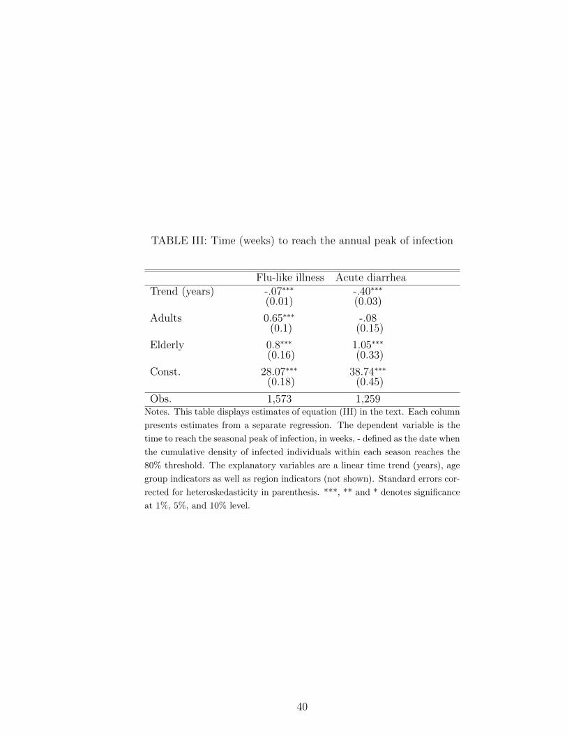
TABLE III: Time (weeks) to reach the annual peak of infection

Flu-like illness Acute diarrheaTrend (years) -.07∗∗∗ -.40∗∗∗

(0.01) (0.03)

Adults 0.65∗∗∗ -.08(0.1) (0.15)

Elderly 0.8∗∗∗ 1.05∗∗∗

(0.16) (0.33)

Const. 28.07∗∗∗ 38.74∗∗∗

(0.18) (0.45)

Obs. 1,573 1,259Notes. This table displays estimates of equation (III) in the text. Each column

presents estimates from a separate regression. The dependent variable is the

time to reach the seasonal peak of infection, in weeks, - defined as the date when

the cumulative density of infected individuals within each season reaches the

80% threshold. The explanatory variables are a linear time trend (years), age

group indicators as well as region indicators (not shown). Standard errors cor-

rected for heteroskedasticity in parenthesis. ***, ** and * denotes significance

at 1%, 5%, and 10% level.

40

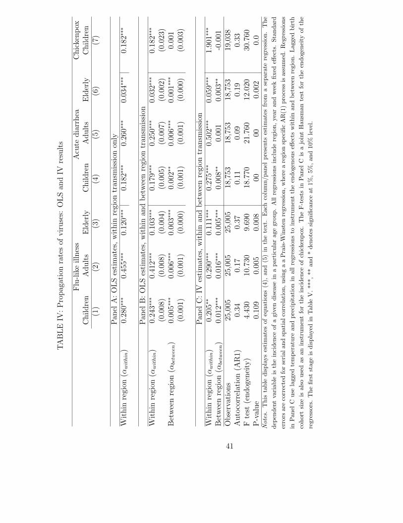
TA

BL

EIV

:P

ropag

atio

nra

tes

ofvir

use

s:O

LS

and

IVre

sult

s

Flu

-lik

eil

lnes

sA

cute

dia

rrh

eaC

hic

ken

pox

Ch

ild

ren

Adu

lts

Eld

erly

Ch

ild

ren

Ad

ult

sE

lder

lyC

hil

dre

n(1

)(2

)(3

)(4

)(5

)(6

)(7

)

Pan

elA

:O

LS

esti

mat

es,

wit

hin

regi

ontr

ansm

issi

onon

lyW

ith

inre

gion

(αwithin

)0.

280∗∗∗

0.45

5∗∗∗

0.12

0∗∗∗

0.18

2∗∗∗

0.26

0∗∗∗

0.03

4∗∗∗

0.18

2∗∗∗

Pan

elB

:O

LS

esti

mat

es,

wit

hin

and

bet

wee

nre

gion

tran

smis

sion

Wit

hin

regi

on(α

within

)0.

243∗∗∗

0.41

2∗∗∗

0.10

3∗∗∗

0.17

9∗∗∗

0.25

0∗∗∗

0.03

2∗∗∗

0.18

2∗∗∗

(0.0

08)

(0.0

08)

(0.0

04)

(0.0

05)

(0.0

07)

(0.0

02)

(0.0

23)

Bet

wee

nre

gion

(αbetween)

0.00

5∗∗∗

0.00

6∗∗∗

0.00

3∗∗∗

0.00

2∗∗

0.00

6∗∗∗

0.00

1∗∗∗

0.00

1(0

.001

)(0

.001

)(0

.000

)(0

.001

)(0

.001

)(0

.000

)(0

.003

)

Pan

elC

:IV

esti

mat

es,

wit

hin

and

bet

wee

nre

gion

tran

smis

sion

Wit

hin

regi

on(α

within

)0.

205∗∗

0.29

0∗∗∗

0.11

1∗∗∗

0.27

5∗∗∗

0.50

2∗∗∗

0.05

9∗∗∗

1.90

1∗∗∗

Bet

wee

nre

gion

(αbetween)

0.01

2∗∗∗

0.01

6∗∗∗

0.00

5∗∗∗

0.00

8∗∗

0.00

10.

003∗∗

-0.0

01O

bse

rvat

ion

s25

,005

25,0

0525

,005

18,7

5318

,753

18,7

5319

,038

Au

toco

rrel

atio

n(A

R1)

0.34

0.17

0.37

0.11

0.09

0.19

0.33

Fte

st(e

nd

ogen

eity

)4.

430

10.7

309.

690

18.7

7021

.760

12.0

2030

.760

P-v

alue

0.10

90.

005

0.00

800

000.

002

0.0

Note

s.T

his

table

dis

pla

ys

esti

mate

sof

equat

ions

(4),

and

(5)

inth

ete

xt.

Eac

hco

lum

n/panel

pre

sents

esti

mate

sfr

om

ase

para

tere

gre

ssio

n.

The

dep

enden

tva

riable

isth

ein

ciden

ceof

agi

ven

dis

ease

ina

par

ticu

lar

age

grou

p.

All

regr

essi

ons

incl

ude

regio

n,

year

and

wee

kfixed

effec

ts.

Sta

ndard

erro

rsare

corr

ecte

dfo

rse

rial

and

spat

ial

corr

elati

on,

usi

ng

aa

Pra

is-W

inst

enre

gre

ssio

n,

wher

ea

regio

nsp

ecifi

cA

R(1

)pro

cess

isass

um

ed.

Reg

ress

ions

inP

anel

Cuse

lagge

dte

mp

eratu

rean

dpre

cipit

atio

nin

all

regre

ssio

ns

toin

stru

men

tth

een

doge

nou

seff

ects

wit

hin

and

bet

wee

nre

gion

.L

agg

edbir

th

cohor

tsi

zeis

als

ouse

das

an

inst

rum

ent

for

the

inci

den

ceof

chic

kenp

ox.

The

F-t

ests

inP

anel

Cis

ajo

int

Hausm

an

test

for

the

endogen

eity

ofth

e

regre

ssor

s.T

he

firs

tst

age

isdis

pla

yed

inT

able

V.

***,

**

and

*den

ote

ssi

gnifi

cance

at

1%

,5%

,an

d10%

leve

l.

41

TABLE V: First stage results: F-tests, p-values and R-square

Children Adults Elderly(1) (2) (3)

Within region (dependent variable: Irt−τSrt−τ )Flu-like illness F-test 3.73 3.71 2.74

p-val (.008) (.008) (.03)

R2 0.272 0.270 0.25Acute diarrhea F-test 5.53 5.53 5.53

p-val (.001) (.001) (.001)

R2 0.55 0.55 0.55Chickenpox F-test 4.08

p-val (.002)

R2 0.32Across regions ( dependent variable:

∑c∈R\r Ict−τSrt−τ )

Flu-like illness F-test 612.30 558.04 501.93p-val (0.0) (0.0) (0.0)

R2 0.417 0.416 0.40Acute diarrhea F-test 1284.12 1258.88 1309.37

p-val (0.0) (0.0) (0.0)

R2 0.8 0.8 0.8Chickenpox F-test 56.52

p-val (0.0)

R2 0.67Notes. The table reports the F test of joint significance of the instruments, with p-values in

parenthesis as well as the R-square of the regression. The dependent variables are defined in

equation (5). Each entry in the table corresponds to a separate regression. The instruments

are lagged cumulative temperature and precipitations within a year (defined as May to

May). For flu-like illnesses and acute diarrhea, the lag is one week. For chickenpox, the

instruments are lagged three weeks, and include also the size of the birth cohorts at regional

level, within the last six years. All regressions include region, year, and week fixed effects.

Robust standard errors are clustered at region level.

42

TA

BL

EV

I:P

ropag

atio

nra

tes

ofvir

use

s:fu

lly

inte

ract

edm

odel

Flu

-lik

eil

lnes

sA

cute

dia

rrh

eaC

hic

ken

pox

Ch

ild

ren

Ad

ult

sE

lder

lyC

hil

dre

nA

du

lts

Eld

erly

Ch

ild

ren

(1)

(2)

(3)

(4)

(5)

(6)

(7)

Pan

elA

.In

terp

erso

nal

conta

cts

Sch

ool

hol

iday

,w

ith

in-.

145∗∗∗

-.10

1∗∗∗

-.00

6-.

071∗∗∗

0.01

40.

01∗∗∗

-.19

7∗∗

(0.019)

(0.019)

(0.008)

(0.009)

(0.013)

(0.004)

(0.078)

Sch

ool

hol

iday

,b

etw

een

-.00

3∗∗∗

-.00

090.

0001

0.00

3∗∗∗

-.00

4∗∗∗

-.00

07∗∗∗

0.00

5(0.0007)

(0.0008)

(0.0003)

(0.0007)

(0.0008)

(0.0003)

(0.004)

Tra

nsp

orta

tion

stri

ke,

wit

hin

-.00

2-.

056∗∗

-.03

6∗∗∗

0.03

80.

016

0.01

7-.

060

(0.026)

(0.024)

(0.011)

(0.026)

(0.039)

(0.012)

(0.154)

Tra

nsp

orta

tion

stri

ke,

bet

wee

n-.

008∗∗

-.01

0∗∗∗

-.00

4∗-.

002

-.00

3-.

001

0.00

9(0.004)

(0.004)

(0.002)

(0.003)

(0.003)

(0.001)

(0.013)

Hig

h-s

pee

dtr

ain

0.00

5∗∗

0.01

4∗∗∗

0.00

7∗∗∗

0.01∗∗∗

0.00

6∗∗∗

0.00

080.

001

(0.003)

(0.002)

(0.001)

(0.002)

(0.002)

(0.0006)

(0.016)

Ad

vers

ew

eath

er,

wit

hin

-.05

0∗∗∗

-.03

5∗∗

0.00

8-.

033∗∗∗

-.00

6-.

0002

-.01

9(0.015)

(0.016)

(0.006)

(0.008)

(0.01)

(0.003)

(0.087)

Pan

elB

:T

rad

eW

ith

inre

gion

0.07

8-.

092

0.00

8-1

.669

-1.3

81∗

-.15

9(0.088)

(0.075)

(0.036)

(4.315)

(0.714)

(0.81)

Bet

wee

nre

gion

s0.

035∗∗∗

0.04

9∗∗∗

0.00

9∗∗

0.01

8∗∗∗

0.02

9∗∗∗

0.00

20.

026

(0.008)

(0.007)

(0.004)

(0.006)

(0.007)

(0.002)

(0.029)

Pan

elC

:U

nem

plo

ym

ent

Wit

hin

regi

on-.

012∗∗

-.00

80.

002

0.00

5-.

014∗∗∗

-.00

10.

004

(0.005)

(0.005)

(0.003)

(0.003)

(0.004)

(0.001)

(0.02)

Bet

wee

nre

gion

s-.

014∗∗∗

0.00

6∗0.

009∗∗∗

0.01∗∗∗

0.00

5-.

002∗∗

0.01

8(0.003)

(0.003)

(0.002)

(0.003)

(0.004)

(0.001)

(0.02)

Tab

leco

nti

nu

edon

nex

tp

age.

43

TA

BL

EV

I:(C

ON

TIN

UE

D)

Flu

-lik

eil

lnes

sA

cute

dia

rrh

eaC

hic

ken

pox

Ch

ild

ren

Ad

ult

sE

lder

lyC

hil

dre

nA

du

lts

Eld

erly

Ch

ild

ren

(1)

(2)

(3)

(4)

(5)

(6)

(7)

Pan

elD

.W

ith

inre

gion

char

acte

rist

ics

Tem

per

atu

re(i

nC

)-.

016∗∗∗

-.02

7∗∗∗

-.00

4∗∗∗

-.00

5∗∗∗

-.00

5∗∗∗

-.00

04-.

004

(0.002)

(0.002)

(0.0009)

(0.0009)

(0.001)

(0.0003)

(0.006)

Pop

ula

tion

den

sity

1.17

3∗∗∗

0.70

1∗∗∗

-.25

2∗∗

0.40

7∗∗∗

-.16

4-.

170∗∗∗

4.44

0∗∗

(0.176)

(0.178)

(0.123)

(0.118)

(0.157)

(0.055)

(1.762)

Pan

elE

.B

etw

een

regi

onch

arac

teri

stic

sD

ista

nce

(100

0km

)0.

0008

0.00

50.

004∗

-.00

4-.

011∗∗∗

-.00

5∗∗∗

0.01

9(0.003)

(0.003)

(0.002)

(0.002)

(0.003)

(0.001)

(0.09)

Pop

ula

tion

rati

o0.

002∗∗

-.00

020.

0009∗∗

0.00

5∗∗∗

0.01∗∗∗

0.00

2∗∗∗

0.02

5∗∗∗

(0.001)

(0.001)

(0.0004)

(0.001)

(0.001)

(0.0004)

(0.006)

Log

GD

Pra

tio

-.00

90.

018∗∗

-.00

07-.

0001

0.06

6∗∗∗

0.01

8∗∗∗

-.05

1(0.01)

(0.009)

(0.004)

(0.008)

(0.009)

(0.003)

(0.042)

Tem

per

atu

reD

iffer

ence

(in

C)

0.00

02∗

0.00

09∗∗∗

0.00

02∗∗∗

0.00

010.

0006∗∗∗

0.00

02∗∗∗

0.00

2∗∗

(0.0001)

(0.0001)

(0.00006)

(0.0001)

(0.0001)

(0.00003)

(0.0007)

Pre

vale

nce

inP

aris

0.04

6∗∗∗

0.04

3∗∗∗

0.01

1∗∗∗

-.00

7∗∗

-.00

30.

003∗∗

0.02

3(0.006)

(0.006)

(0.003)

(0.003)

(0.004)

(0.001)

(0.016)

Ob

serv

atio

ns

24,4

0724

,407

24,4

0718

,537

18,5

3718

,537

17,6

02R

-squ

ared

0.57

0.73

0.37

0.54

0.67

0.27

0.24

Note

s.T

his

table

dis

pla

ys

esti

mate

sof

the

para

met

ersαk within

andαk betw

een

defi

ned

ineq

uati

on

(6)

inth

ete

xt.

Each

colu

mn

repre

sents

ase

para

te

regre

ssio

nw

ith

inci

den

cera

tes

asth

edep

enden

tva

riable

s.P

anel

sar

eor

ganis

edfo

rea

seof

exp

osi

tion,

but

all

the

vari

able

slist

edin

the

table

are

incl

uded

inth

ere

gre

ssio

n.

Inaddit

ion,

the

regre

ssio

ns

contr

olfo

rre

gio

n,

year

and

wee

kfixed

effec

tsin

level

sand

regi

on

fixed

effec

ts,

quart

erly

dum

mie

sand

alinea

rtr

end

inte

ract

edw

ith

tran

smis

sion

rate

s.L

agg

edte

mp

erat

ure

and

pre

cipit

ati

onar

euse

das

inst

rum

ents

inall

regre

ssio

ns

to

inst

rum

ent

the

endogen

ous

effec

tsw

ithin

and

bet

wee

nre

gion

.L

agge

dbir

thco

hor

tsi

zeis

als

ouse

das

an

inst

rum

ent

for

the

inci

den

ceof

chic

kenp

ox.

Sta

ndard

erro

rsar

eco

rrec

ted

for

seri

alan

dsp

ati

alco

rrel

atio

n,

usi

ng

aa

Pra

is-W

inst

enre

gre

ssio

n,

wher

ea

regio

nsp

ecifi

cA

R(1

)pro

cess

isass

um

ed.

***

,**

and

*den

ote

ssi

gnifi

cance

at1%

,5%

,and

10%

leve

l.

44

TABLE VII: Costs of disease per case, influenza

ChildrenGP visit (32% chance) 6.68 eOtitis media (0.28% chance) 17.38 ePneumonia (12% chance) 16.45 eHospitalisation (0.07% chance) 2.45 eHospitalisation (sequelae pneumonia 0.7 per 100,000) 3.61 eLoss of human capital (3 days off school, 5% return) 99 eParent stays home (50% of time, labor market particip. 0.65) 102 eValue of statistical life 1.3-6 million eProbability of death 0.7 per 100,000Cost of death 9-42 e

AdultsAbsent from work (2 days of work at average wage) 78.90eReduced productivity (0.7 days at 50%) 13.80 eGP visit (45% chance) 9.45 eHospitalisation (0.04% chance) 1.80 eValue of statistical life 1.3-6 million eProbability of death 4 per 100,000Cost of death 52-240 e

ElderlyOutpatient visit 219 eHospital 476 eValue of statistical life 1.3-6 million eProbability of death 102 per 100,000Cost of death 1326-6120 e

Notes. Data on costs and healthcare use are taken from Prosser et al. (2006) for children,

from Nichol (2001) for adults and from Molinari et al. (2007) for the elderly. These studies

weight medical costs by the probability of health care usage. Data on mortality from in-

fluenza by age group comes from the National Vital Statistics Report 2011. Data on wages

are taken from INSEE, “Revenus salariaux medians des salaries de 25 a 55 ans selon le sexe en

2011” (http://www.insee.fr/fr/themes/tableau.asp?reg id=0&ref id=NATnon04146). La-

bor market participation data comes from OECD skill data set. All US dollars converted

into euros with an exchange rate of 0.8. Loss of human capital is costed using a return

to schooling of 5 percent, median wages by sex and average labor market participation by

sex over a period of 42 years. Net present value numbers are displayed, calculated with a

discount factor equal to 0.95.

45

TABLE VIII: Costs of disease per case, acute diarrhea

ChildrenMedication, GP visits 3.16 eHospitalisation 5.4 eLoss of human capital (2 days off school, 5% return) 66 eAbsence of other person for informal care 57 eValue of statistical life 1.3-6 million eProbability of death 0.4 per 100,000Cost of death 5.2-24 e

AdultsWork absence 105.8 eMedication, GP visits 2.61 eHospitalisation 5.15 eValue of statistical life 1.3-6 million eProbability of death 0.5 per 100,000Cost of death 6-30 e

ElderlyMedication, GP visits 16.3 eHospitalisation 83 eValue of statistical life 1.3-6 million eProbability of death 22 per 100,000Cost of death 286-1320 eNotes. Data on costs and healthcare use are taken from Van Den Brandhof

et al. (2004). Medical costs are weighted by the probability of health care us-

age. Data on mortality from acute diarrhea by age group comes from the Na-

tional Vital Statistics Report 2011. Data on wages are taken from INSEE,

“Revenus salariaux medians des salaries de 25 a 55 ans selon le sexe en 2011”

(http://www.insee.fr/fr/themes/tableau.asp?reg id=0&ref id=NATnon04146). Labor mar-

ket participation data comes from OECD skill data set. All costs are adjusted for inflation

and in 2005 euros. US dollars converted into euros with an exchange rate of 0.8. Loss

of human capital is costed using a return to schooling of 5 percent, median wages by sex

and average labor market participation by sex over a period of 42 years.Net present value

numbers are displayed, calculated with a discount factor equal to 0.95.

46

TABLE IX: Cost of policy, euros per capita

School closure10 days off school, return to schooling, 5% per year 350 eParent stays home (50% of time, labor market particip. 0.65) 150 e

Public transportation closuree400 million per week 19 e

Notes. Data on wages are taken from INSEE, “Revenus salari-

aux medians des salaries de 25 a 55 ans selon le sexe en 2011”

(http://www.insee.fr/fr/themes/tableau.asp?reg id=0&ref id=NATnon04146). La-

bor market participation data comes from OECD skill data set. Cost of public

transportation closure comes from Dubois et al. (2007).

47

Figure I: Weekly incidence rates, 1984-2010

0500

1000

1500

2000

Infe

ction r

ate

per

100,0

00

1985w1 1990w1 1995w1 2000w1 2005w1 2010w1Week

Flu−like Illnesses

0200

400

600

800

Infe

ction r

ate

per

100,0

00

1990w1 1995w1 2000w1 2005w1 2010w1Week

Acute Diarrhea0

20

40

60

Infe

ction r

ate

per

100,0

00

1990w1 1995w1 2000w1 2005w1 2010w1Week

Chickenpox

Notes. Data from InVS. Infection rates per 100,000 individuals.

48

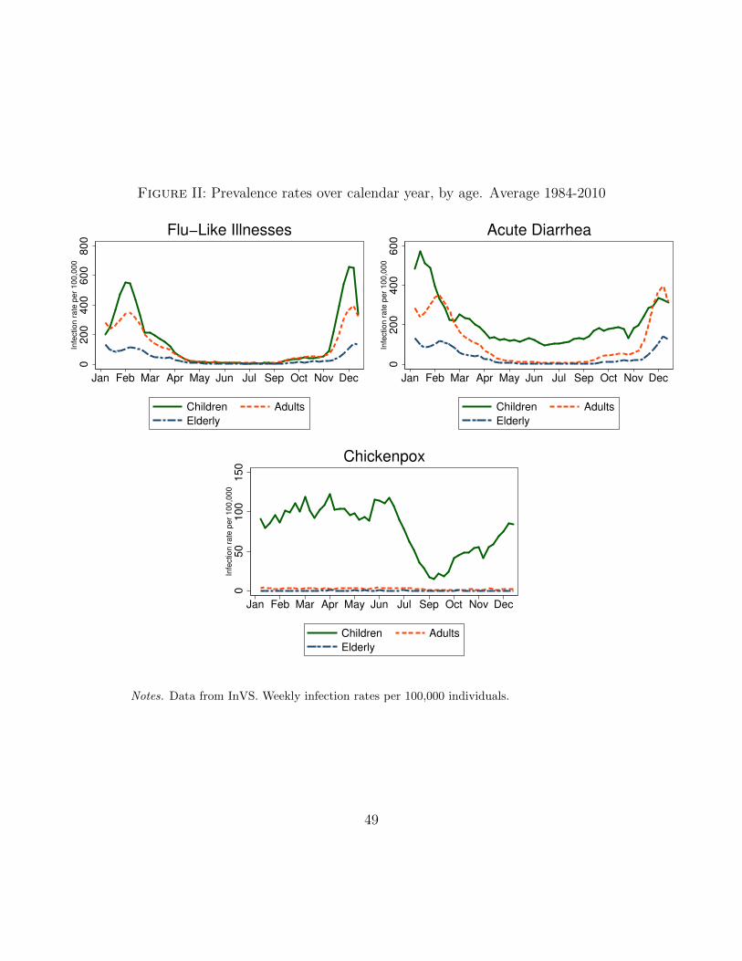
Figure II: Prevalence rates over calendar year, by age. Average 1984-2010

0200

400

600

800

Infe

ction r

ate

per

100,0

00

Jan Feb Mar Apr May Jun Jul Sep Oct Nov Dec

Children Adults

Elderly

Flu−Like Illnesses

0200

400

600

Infe

ction r

ate

per

100,0

00

Jan Feb Mar Apr May Jun Jul Sep Oct Nov Dec

Children Adults

Elderly

Acute Diarrhea0

50

100

150

Infe

ction r

ate

per

100,0

00

Jan Feb Mar Apr May Jun Jul Sep Oct Nov Dec

Children Adults

Elderly

Chickenpox

Notes. Data from InVS. Weekly infection rates per 100,000 individuals.

49

Figure III: Public Transportation Strikes, France, 1984-2010

(a) Frequency within Year

0.0

2.0

4.0

6.0

8F

req

ue

ncy o

f T

rain

Str

ike

s

Jan Feb Mar Apr May Jun Jul Aug Sep Oct Nov Dec

(b) Frequency by Duration

0.0

1.0

2.0

3.0

4.0

5D

en

sity

0 10 20 30 40 50

Duration (in Days)Average Duration: 12.3 days; Median duration 8 days.

Notes. Data collected by the author using the LexisNexis search of the French written press.

All occurrences of a public transportation strike lasting three days at least, either nationally

or regionally were recorded from the national press (Le Monde, Le Figaro).

50

Figure IV: Expansion of the high speed railway

RENNES

CAEN ROUEN

AMIENS

LILLE

CHALONS-EN-C

METZ

STRASBOURG

BESANCONDIJON

LYON

MONTPELLIER

BORDEAUX

TOULOUSE

POITIERS

NANTES

ORLEANS

PARIS

LIMOGESCLERMONT-FER

MARSEILLE

Sept 1989

Sept 1990

June 2007

May 1993

Sept 1981

May 1994

Jun 2001

Sept 1989Jan 1984

Notes. The map displays the major connections of the high-speed rail link in France and

the date of opening. To avoid cluttering, only direct links are displayed. The analysis also

takes into account opening of links between two cities where a stop in Paris was no longer

necessary, e.g. Marseille - Lille without change of trains in Paris.

51

Figure V: Event Analysis: School Closures

(a) Flu-like illnesses, children

.6.7

.8.9

11

.11

.21.3

No

rma

lise

d P

reva

len

ce

−4 −2 0 2 4 6Weeks since Start of School Closure

(b) Flu-like illnesses, adults

.6.7

.8.9

11

.11

.21.3

No

rma

lise

d P

reva

len

ce

−4 −2 0 2 4 6Weeks since Start of School Closure

(c) Flu-like illnesses, elderly

.6.7

.8.9

11

.11

.21.3

No

rma

lise

d P

reva

len

ce

−4 −2 0 2 4 6Weeks since Start of School Closure

(d) Acute diarrhea, children

.8.9

11

.11

.2N

orm

alis

ed

Pre

va

len

ce

−4 −2 0 2 4 6Weeks since Start of School Closure

(e) Acute diarrhea, adults

.8.9

11

.11

.2N

orm

alis

ed

Pre

va

len

ce

−4 −2 0 2 4 6Weeks since Start of School Closure

(f) Acute diarrhea, elderly

.8.9

11

.11

.2N

orm

alis

ed

Pre

va

len

ce

−4 −2 0 2 4 6Weeks since Start of School Closure

(g) Chickenpox, children

.7.8

.91

1.1

1.2

No

rma

lise

d P

reva

len

ce

−4 −2 0 2 4 6Weeks since Start of School Closure

The different panels display the estimates of equation (2) and show the weekly incidence of the diseasewithin a region as a function of the time since the first week of school holidays. Results obtained froma regression controlling also for region, year and week effects. Standard errors are clustered by region.The incidence is normalised by the average incidence one week before the strike (labelled as -1). Schoolclosures last typically for one or two weeks, except for the 8 week summer break. Solid line is the meaneffect by week, 95 percentiles are shown as vertical bars.

52

Figure VI: Event Analysis: Public Transportation Strike

(a) Flu-like illnesses, children

.2.4

.6.8

11

.21.4

1.6

No

rma

lise

d P

reva

len

ce

−4 −2 0 2 4Weeks since Start of Public Transportation Strike

(b) Flu-like illnesses, adults

.2.4

.6.8

11

.21

.41

.6N

orm

alis

ed

Pre

va

len

ce

−4 −2 0 2 4Weeks since Start of Public Transportation Strike

(c) Flu-like illnesses, elderly

.2.4

.6.8

11

.21

.41

.6N

orm

alis

ed

Pre

va

len

ce

−4 −2 0 2 4Weeks since Start of Public Transportation Strike

(d) Acute diarrhea, children

.4.6

.81

1.2

1.4

1.6

No

rma

lise

d P

reva

len

ce

−4 −2 0 2 4Weeks since Start of Public Transportation Strike

(e) Acute diarrhea, adults

.4.6

.81

1.2

1.4

1.6

No

rma

lise

d P

reva

len

ce

−4 −2 0 2 4Weeks since Start of Public Transportation Strike

(f) Acute diarrhea, elderly

.4.6

.81

1.2

1.4

1.6

No

rma

lise

d P

reva

len

ce

−4 −2 0 2 4Weeks since Start of Public Transportation Strike

The different panels display the estimates of equation (2) and show the weekly incidence of thedisease within a region as a function of the time since the first week of a public transportation strike.Results obtained from a regression controlling also for region, year and week effects. Standarderrors are clustered by region. The incidence is normalised by the average incidence one weekbefore closure (labelled as -1). Solid line is the mean effect by week, 95 percentiles are shown asvertical bars. Chickenpox is omitted as transportation strikes do not have statistically significanteffects.

53

Figure VII: Effect of policy measures on annual disease prevalence, by week of imple-mentation

(a) Flu-like illness and school closure

Week of extra school closureSep Oct Nov Dec Jan Feb Mar Apr May Jun Jul Aug

Re

du

ctio

n in

an

nu

al p

reva

len

ce

0.86

0.88

0.9

0.92

0.94

0.96

0.98

1

(b) Acute diarrhea and school closure

Week of extra school closureSep Oct Nov Dec Jan Feb Mar Apr May Jun Jul Aug

Re

du

ctio

n in

an

nu

al p

reva

len

ce

0.96

0.965

0.97

0.975

0.98

0.985

0.99

0.995

1

(c) Flu-like illness and publictransportation closure

Week of public transportation shutdowmSep Oct Nov Dec Jan Feb Mar Apr May Jun Jul Aug

Reduction in a

nnual pre

vale

nce

0.92

0.93

0.94

0.95

0.96

0.97

0.98

0.99

1

(d) Acute diarrhea and public trans-portation closure

Week of public transportation shutdowmSep Oct Nov Dec Jan Feb Mar Apr May Jun Jul Aug

Re

du

ctio

n in

an

nu

al p

reva

len

ce

0.982

0.984

0.986

0.988

0.99

0.992

0.994

0.996

0.998

1

Notes. The different panels display the annual prevalence of diseases as a function of the week

of implementation of the policy. The prevalence are in deviation from a baseline scenario, which

includes school closures due to regular holidays. School closures lasts for two weeks and public

transportation closures for one week. The discontinuous lines in Panels (a) and (b) are due to

periods of holidays, when schools are closed anyway. The results are based on estimated coefficients

of equation (6) and shown in Table VI. The results were averaged over 500 replications, drawing

realisations for the shock in equation (6) and for the estimated coefficients from their asymptotic

distribution.

54

Figure VIII: Overall gain of policy measures closures, by week of implementation

(a) School closure

Week of extra school closureSep Oct Nov Dec Jan Feb Mar Apr May Jun Jul Aug

Gain

in e

uro

s p

er

capita

-40

-35

-30

-25

-20

-15

-10

-5

0

(b) Public transportation closure

Week of transportation closureSep Oct Nov Dec Jan Feb Mar Apr May Jun Jul Aug

Gain

in e

uro

s p

er

capita

-20

-18

-16

-14

-12

-10

-8

-6

-4

-2

0

Notes. The different panels display the gain in per capita euros of the policy compared to a baseline

scenario, which includes school closures due to regular holidays. The calculations use a value of statistical

life equal to 5 million euros regardless of age. The results are based on estimated coefficients of equation (6)

and cost measures displayed in Tables VII, VIII and IX. The results were averaged over 500 replications,

drawing realisations for the shock in equation (6) and for the estimated coefficients from their asymptotic

distribution.

55

Appendix

A Supplementary Data Description

Data on viral diseases The data on viral diseases is collected by the Institut deVeille Sanitaire (InVS) on a continuous basis from 1984. It relies on information sent bya network of GPs across the whole country. The network represents about 1-2 percentof all French GPs over the period we analyze. These doctors are representative of thepopulation of active GPs. Figure I depicts the geographical dispersion of these GPs in2006. Each dot indicates the localisation of a particular GP. The network is more densein the Paris area, as well as along the Mediterranean coast, which corresponds to areaswith higher population density.

Figure I: Density of General Practitioners belonging to the Reseau Sentinelles, 2006Source: InVS (2006)

The doctors report all cases of particular diseases, on a daily to weekly basis througha web/electronic interface. Prior to the existence of the internet and computers, doc-tors were equipped with an electronic terminal (Minitel) allowing them to send data.The data are then compiled by the InVS to produce incidence rates by region and

56

by age groups, using additional data on the number of general practitioners and thesize of demographic groups by area derived from the French census. The French cen-suses took place in 1982, 1990 and 1999 in an exhaustive way. Since 2004, the cen-sus is updated every year, based on a random survey. The incidence rates are cal-culated, assuming that conditional on observables, the doctors are randomly selected.The data and information on how the data is constructed is available from the InVS(http://www.invs.sante.fr) and is described in more detail in Flahault et al. (2006).

Weather Data: We obtained daily temperatures from the European Climate As-sessment and Dataset (Tank et al. (2002)) for the period 1984-2010. We aggregate thetemperature at a weekly level to make it consistent with the data on disease incidences.The data was obtained for major cities in France and we allocate each city to a region.In the case where more than one reading was obtained for a region, we took the data forthe most populous city. In case there is no reading for a particular region, we linearlyinterpolated the data between the two nearest stations.

Population Data: The data were extracted from the French census conducted byINSEE for each region and linearly interpolated for the missing years. Data on cohortsize was gathered from INSEE, for each region and year between 1975 and 2010.

Trade data: The data come from the French Comissariat General au DeveloppementDurable and describe the intra and inter-regional transportation of goods, expressedin metric tons per year. For each region, the data report the quantities transportedwithin the region and to all other regions by road, rail or boat (a number of regionsare connected by rivers or canals). The data span the period 1975 to 2011, exceptfor rail transportation which only goes to 2006. To get consistent measures acrossyears, we use the sum of quantities transported by road and boat and discard theinformation on rail transport. Rail transportation of goods represents about 20% of allgoods transported. Nevertheless, the measure we use is highly correlated with the totaltransportation measure for the years 1975-2006, where we have the data for all meansof transportation. The overall correlation is equal to 0.997 and the correlations withinorigin-destination region pairs are also very close to one (the median correlation amongthe 21*21 measures is 0.98).

57

B Computation of the Susceptible Population

in the case of Chickenpox

We denote nbrt the size of the cohort born in year t in region r. We abstract from infantmortality as well as regional migration, so that the cohort does not vary (substantiallyand systematically) in size over the first J years. We denote by ρrt the fraction ofchildren who contract chickenpox in year t and region r out of the pool of children atrisk. The susceptible population consist of the sum of all children for each birth cohortthat have not yet been infected, starting with the newborns, up to the children of ageJ .28

Srt = nbrt + (1− ρrt−τ )nbrt−τ + . . .+J∏c=1

(1− ρrt−c)nbrt−J . (1)

We assume that at age J+1, all children have been exposed to the disease. The numberof new cases in year t and region r is:

Irt = ρrtSrt.

We compute the size of the susceptible population using the history of disease in-cidence as well as data on the size of the birth cohorts, by region and year. Thecomputation proceeds iteratively. Note that we can write the propensity to becomeinfected as:

ρrt =Irt

nbrt + (1− ρrt−τ )nbrt−τ + . . .+J∏c=1

(1− ρrt−c)nbrt−J(2)

We first focus on the stationary equilibrium which is used as an initial guess in theiterative procedure. With a stable population and no variations in the infectiousnessof the disease, one can solve for the stationary solution ρ as a function of the numberof cases and the size of the birth cohort:

ρr = 1−(

1− Irnbr

)1/J+1

28In practice, we set this parameter to 16 for two reasons. First, the disease is predominant inyoung children, with a median age of about 6 years old (Guris et al. (2008)) and the incidence ofdiseases is extremely small for an adult population (see Figure II). Second, the data on the size of thebirth cohorts starts in 1975, and setting J = 16 allows us to calculate the population of susceptibleindividuals from the start of our data set describing the incidence in 1991.

58

This value can be used to compute a first guess of the susceptible population usingequation (1), combining data on incidence and size of various cohorts, for all periods inthe data set. At the nth iteration, the set of propensities to become infected verifies:

ρnrt =Irt

Srt(ρn−1rt )

We repeat this procedure until convergence, which, practically, occurs very quickly. Wethen check that Irt(ρ

nrt) is indeed close to the observed incidence of the disease in that

region and time period. We are able to match these data very closely, with a correlationequal to 0.993.

C Measurement error

We show in this section how measurement error affects the estimation of equation (5).Denote the observed incidence rate as: Irt = Irt + εrt, where εrt is the error, arisingfrom the fact the incidence of diseases are estimated from the number of cases seenby a network of general practitioners, which is subject to sampling error. This errormay not be classical. It is possible that the incidence rate is more likely measured witherror when the incidence is very high, and patients have to queue to see a doctor. Themeasurement error on the incidence rate also affects the measurement of the proportionof susceptible individuals. Taking into account the measurement error, we can rewriteequation (5) expressed with observed variables as

Irt = αwithinIrt−τ Srt−τ + αbetween∑c∈R\r

Ict−τ Srt−τ +Xrtδ + ηrt (3)

The error term depends on the disease into consideration as it implies different defi-nitions of the susceptible population. In the simple case of gastroenteritis, where wedefine the susceptible population as Srt = Nrt − Irt−τ , i.e. the total population minusthose who were sick the week before, the error term is expressed as:

ηrt = ηrt + εrt − αwithinSrt−τ εrt−τ + αwithinIrt−τεrt−2 − αwithinεrt−τεrt−2

+αbetween

εrt−2 ∑c∈R\r

(Ict−τ − εct−τ

)− Srt−τ

∑c∈R\r

εct−τ

(4)

In the case of influenza and chickenpox, the error term is more complex as the sus-ceptible population consists of an estimate of all those who have been infected during

59

the flu season or in the preceding years. For these two diseases, the error term con-tains measurement error terms over a longer period than gastroenteritis. In all cases,measurement error implies a complex structure for the error term, which exhibit se-rial correlation and heteroskedasticity. Importantly, given this structure, we cannotexclude the possibility that cov(Irt−1Srt−1, ηrt) 6= 0, which leads to biased inference ofthe parameters of interest.

D Robustness of results and further evidence

In this section, we explore additional departures from our model (6). We investigateheterogeneous effects with respect to the lagged incidence of the disease and we test forinteractions between diseases.

DA. Non-linear effects

We first look at non-linear effects of lagged incidence rate by looking at various quan-tiles. The standard epidemiological model interacts the lagged incidence (Irt−1 in ournotations in equation (6)) with the size of the susceptible population (Srt−1). There isa priori no reason for this particular matching function to be expressed as the prod-uct of these two variables, in a geometric way. We explore whether transmission ratesvary with the level of the lagged incidence rate, which is equivalent to postulating thatthe matching function can be expressed as f(Irt−1)Srt−1, which generalises our model.Another reason for a non-linear relationship can be due to behavioral adjustment. Sus-ceptible individuals may observe incidence rates and avoid getting into contact withpotentially sick individuals. In this case the function f() is decreasing in the incidencerate.

We allow the parameter (or matrix of parameters) α to vary, and we discretisethe lagged incidence into 6 intervals, denoted [Iq, Iq+1]. We denote 1Irt−τ∈[Iq ,Iq+1] anindicator variable equal to one when the incidence in region r and period t− τ is withinthe corresponding interval.

Irt =6∑q=1

1Irt−τ∈[Iq ,Iq+1]

αqwithinIrt−τSrt−τ + αqbetween∑c∈R\r

Ict−τSrt−τ

+Xrtδ + ηrt (5)

We are particularly interested in episodes with high incidence, which are more rel-evant for policy. We display in the appendix Table II, Panel A the intercept for thetransmission within a region. We find some evidence that the transmission rate ishigher, the higher the lagged incidence rate of the disease, especially for increasing

60

ages. For children, however, the confidence intervals tend to overlap, suggesting thatthe baseline model fits the data well. We find similar patterns for transmissions acrossregions, displayed in Table II, Panel B. These results do not offer much support forbehavioral adjustment, where the transmission rate would be lower the higher the pastincidence. However, to fully investigate this aspect, more precise data on actual behav-ior would be required.

DB. Interactions across diseases

We estimate a model where we allow for the incidence rate of acute diarrhea to influencethe effect on how flu-like illnesses are transmitted and vice-versa. There can be twoopposite effects, an incapacitation one, which limits the propagation of the other diseaseas sick individuals tend to stay home, and a weakening effect that enhances the effectof a given disease. The results are displayed in the appendix Table III and the resultsare to be interpreted as the effect of a standard deviation increase in the incidence ofa disease on the transmission rate of the other disease. Sadly, the weakening effectappears to dominate in the case of flu-like illnesses which propagate faster when moreindividuals suffer from acute diarrhea, at least for adults and the elderly. We also findsimilar effects for all age groups in the case of transmission of acute diarrhea during flu-like illnesses outbreak. No such effect can be seen in the transmission rate of chickenpox.We find therefore similar interactions effects across diseases as in Oster (2005), althoughthe channel would be quite different. From a public health point of view, this is badnews as one epidemic tend to reinforce the other.

DC. Cost of policy measures

We provide further detail on the cost of policy measures studied in Section V.. Theappendix Table IV assess the robustness of the results to the value of statistical life.We use values ranging from 1.3 to 6 million euros, which correspond to the range foundin the literature. Our results are broadly insensitive to the different values, except forvery low values for flu-like illnesses in the case of public transportation closures.

61

TA

BL

EI:

Fir

stSta

geR

esult

s,W

ithin

Reg

ion

Var

iable

s

Flu

-lik

eilln

ess

Acu

tedia

rrhea

Chic

kenp

oxC

hildre

nA

dult

sE

lder

lyC

hildre

nA

dult

sE

lder

lyC

hildre

n(1

)(2

)(3

)(4

)(5

)(6

)(7

)W

eeks

wit

hte

mp<

0C22

3.66

5***

210.

473*

**10

9.10

9***

83.3

2783

.488

83.6

09-1

1.53

4(5

5.08

3)(5

0.86

3)(2

8.41

8)(5

3.99

7)(5

4.01

9)(5

4.10

5)(1

1.20

8)W

eeks

wit

hte

mp<

5C-3

7.77

7*-3

2.97

5*-4

.659

-31.

785

-31.

890

-32.

008

-1.7

88(2

0.24

6)(1

9.04

7)(1

3.19

3)(2

0.26

9)(2

0.29

7)(2

0.34

7)(3

.177

)W

eeks

wit

hte

mp<

10C

99.4

46**

91.2

00**

30.4

8840

.847

**41

.079

**41

.192

**-1

.370

(41.

980)

(39.

042)

(21.

844)

(18.

572)

(18.

579)

(18.

642)

(4.0

74)

Wee

ks

wit

hte

mp>

15C

-14.

431

-19.

766

-28.

083

89.1

77**

89.4

33**

89.7

12**

5.45

4(5

3.00

1)(5

0.29

4)(2

4.96

2)(3

1.92

4)(3

1.95

6)(3

2.01

4)(4

.512

)W

eeks

wit

hte

mp>

20C

-39.

658

-34.

258

5.47

14.

560

4.36

84.

342

2.10

0(2

9.93

8)(2

9.08

7)(2

3.51

9)(4

8.10

4)(4

8.19

0)(4

8.28

5)(3

.370

)W

eeks

wit

hte

mp>

25C

-75.

856

-74.

756

39.4

8212

0.15

212

0.39

912

0.94

96.

290

(132

.059

)(1

28.3

72)

(93.

359)

(129

.444

)(1

29.7

29)

(130

.099

)(1

1.95

7)R

ainfa

llin

last

4w

eeks

-157

.950

**-1

42.2

75**

-65.

663*

-74.

804*

**-7

4.72

6***

-75.

053*

**3.

972*

(72.

614)

(66.

801)

(31.

548)

(24.

878)

(24.

917)

(24.

967)

(2.1

75)

Rai

nfa

llin

last

8w

eeks

-57.

777

-63.

217

-47.

487

133.

778*

*13

3.63

7**

134.

092*

*-7

.968

*(6

3.74

1)(5

8.98

1)(3

2.82

0)(5

1.33

1)(5

1.43

9)(5

1.59

4)(3

.856

)N

ewb

orns

inre

gion

,ye

art

-0.0

00(0

.004

)N

ewb

orns

inre

gion

,ye

art-

10.

001

(0.0

04)

New

bor

ns

inre

gion

,ye

art-

20.

001

(0.0

04)

New

bor

ns

inre

gion

,ye

art-

3-0

.009

(0.0

16)

New

bor

ns

inre

gion

,ye

art-

40.

021

(0.0

17)

New

bor

ns

inre

gion

,ye

art-

5-0

.034

***

(0.0

11)

New

bor

ns

inre

gion

,ye

art-

60.

040*

**(0

.008

)O

bse

rvat

ions

2571

025

710

2571

019

146

1914

619

146

1977

0R

-squar

ed0.

272

0.27

00.

251

0.54

70.

547

0.54

70.

324

Tab

leco

nti

nued

onnex

tpag

e.

62

TA

BL

EI:

(CO

NT

INU

ED

),B

etw

een

Reg

ion

Var

iable

s

Flu

-lik

eil

lnes

sA

cute

dia

rrh

eaC

hic

ken

pox

Ch

ild

ren

Ad

ult

sE

lder

lyC

hil

dre

nA

du

lts

Eld

erly

Ch

ild

ren

(1)

(2)

(3)

(4)

(5)

(6)

(7)

Reg

ion

sw

ith

tem

p<

051

97.4

22**

*48

61.7

47**

*30

35.8

55**

*64

4.64

1***

641.

847*

**64

3.69

3***

21.5

08**

*(9

2.20

7)(8

9.32

3)(5

1.17

1)(3

3.03

6)(3

2.64

7)(3

2.31

0)(2

.705

)R

egio

ns

wit

hte

mp<

1071

7.39

1***

675.

270*

**40

4.44

2***

363.

595*

**36

5.40

0***

365.

959*

**0.

202

(31.

895)

(30.

018)

(15.

502)

(12.

273)

(12.

284)

(12.

316)

(2.0

61)

Reg

ion

sw

ith

tem

p<

2013

8.32

0***

144.

402*

**27

7.03

0***

-3.9

17-4

.133

-4.3

50-6

7.47

0***

(27.

593)

(25.

164)

(14.

319)

(16.

073)

(16.

114)

(16.

133)

(4.1

23)

Wee

ks

tem

per

atu

re<

0C28

98.4

68**

*27

52.9

72**

*11

83.4

57**

149.

746

152.

689

154.

802

-20.

295

(850

.651

)(7

89.6

56)

(450

.970

)(1

52.8

95)

(153

.027

)(1

53.4

41)

(42.

014)

Wee

ks

tem

per

atu

re<

5C93

.986

113.

636

357.

999*

-112

.485

-113

.314

-114

.792

24.8

41(3

40.4

67)

(308

.929

)(1

93.7

77)

(116

.153

)(1

16.1

83)

(116

.162

)(2

0.76

6)W

eeks

tem

per

atu

re<

10C

324.

209

277.

901

-211

.724

-304

.009

**-3

01.9

42**

-301

.735

**51

.100

*(3

46.1

28)

(325

.039

)(1

81.0

06)

(135

.142

)(1

34.9

04)

(135

.025

)(2

5.47

3)W

eeks

tem

per

atu

re>

15C

-768

.818

*-8

06.1

84*

-656

.123

***

1108

.189

***

1109

.753

***

1113

.363

***

96.9

34**

*(4

03.0

75)

(399

.076

)(2

27.4

92)

(147

.357

)(1

46.7

93)

(146

.769

)(2

2.58

6)W

eeks

tem

per

atu

re>

20C

-293

.220

-223

.112

365.

054

814.

980*

**81

4.54

5***

814.

854*

**68

.499

**(4

09.8

59)

(393

.466

)(2

32.3

49)

(126

.865

)(1

27.3

56)

(127

.518

)(2

9.44

7)W

eeks

tem

per

atu

re>

25C

-377

1.85

0***

-360

8.75

6***

-149

3.34

8***

-478

.493

-478

.492

-474

.643

-49.

846

(659

.066

)(6

31.1

53)

(367

.159

)(3

53.3

71)

(352

.091

)(3

53.3

93)

(41.

877)

Rai

nfa

llin

last

4w

eeks

-148

2.09

6*-1

286.

211*

-398

.239

-608

.933

***

-607

.601

***

-611

.145

***

43.3

41**

*(7

17.2

45)

(668

.429

)(3

48.3

19)

(149

.681

)(1

50.3

43)

(150

.478

)(1

0.39

9)R

ain

fall

inla

st8

wee

ks

-221

6.68

1***

-221

8.76

6***

-135

8.27

3***

1312

.478

***

1311

.016

***

1316

.546

***

-29.

057

(696

.852

)(6

76.0

10)

(375

.703

)(4

33.5

02)

(433

.653

)(4

34.5

52)

(30.

646)

New

bor

ns

inre

gion

,ye

art

-0.0

03(0

.013

)N

ewb

orn

sin

regi

on,

year

t-1

0.01

2*(0

.006

)N

ewb

orn

sin

regi

on,

year

t-2

0.04

2***

(0.0

09)

New

bor

ns

inre

gion

,ye

art-

3-0

.125

***

(0.0

32)

New

bor

ns

inre

gion

,ye

art-

40.

104*

*(0

.043

)N

ewb

orn

sin

regi

on,

year

t-5

0.00

4(0

.022

)N

ewb

orn

sin

regi

on,

year

t-6

-0.0

88**

*(0

.023

)O

bse

rvat

ion

s25

710

2571

025

710

1914

619

146

1914

619

811

R-s

qu

ared

0.41

70.

416

0.39

70.

796

0.79

70.

797

0.66

8

Note

s.T

his

table

dis

pla

ys

esti

mate

sof

the

firs

tst

age

regr

essi

ons

for

the

wit

hin

and

the

bet

wee

nre

gio

nva

riable

s,as

ineq

uati

on

(5).

Each

colu

mn

repre

sents

ase

para

tere

gre

ssio

nw

ith

inci

den

ceti

mes

the

num

ber

ofsu

scep

tible

indiv

iduals

as

the

dep

enden

tva

riable

s.T

he

inst

rum

ents

rela

ting

to

wea

ther

are

lagged

,w

ith

ala

gof

one

wee

kfo

rflu-l

ike

illn

esse

sand

acu

tedia

rrhea

and

thre

ew

eeks

inth

eca

seof

chic

kenp

ox.

All

regre

ssio

ns

incl

ude

regio

n,

year

and

wee

kfixed

effec

ts.

Sta

ndar

der

rors

are

clust

ered

at

regi

onal

level

.***,

**

and

*den

ote

ssi

gnifi

cance

at1%

,5%

,and

10%

leve

l.

63

TA

BL

EII

:N

on-l

inea

reff

ects

ofla

gged

inci

den

ce,

by

quan

tile

sof

inci

den

ce,

wit

hin

regi

on

Flu

-lik

eil

lnes

sA

cute

dia

rrh

eaC

hic

ken

pox

Ch

ild

ren

Ad

ult

sE

lder

lyC

hil

dre

nA

du

lts

Eld

erly

Ch

ild

ren

(1)

(2)

(3)

(4)

(5)

(6)

(7)

Pan

elA

:w

ith

inre

gion

effec

ts(α

q within

)

Qu

anti

le[0

-25]

0.3

0.18

60.

025

0.25

2∗∗∗

0.31∗∗∗

0.03

31.

584∗∗∗

(0.184)

(0.19)

(0.098)

(0.055)

(0.068)

(0.022)

(0.371)

Qu

anti

le[2

5-50

]0.

303∗∗∗

0.27

8∗∗∗

0.08

1∗0.

244∗∗∗

0.30

9∗∗∗

0.02

71.

714∗∗∗

(0.094)

(0.1)

(0.044)

(0.054)

(0.066)

(0.021)

(0.364)

Qu

anti

le[5

0-75

]0.

359∗∗∗

0.32

7∗∗∗

0.04

40.

222∗∗∗

0.32∗∗∗

0.03

5∗1.

603∗∗∗

(0.069)

(0.074)

(0.031)

(0.053)

(0.064)

(0.021)

(0.363)

Qu

anti

le[7

5-90

]0.

502∗∗∗

0.42

7∗∗∗

0.07

5∗∗∗

0.23

7∗∗∗

0.38

2∗∗∗

0.04

4∗∗

1.67

5∗∗∗

(0.063)

(0.067)

(0.028)

(0.054)

(0.065)

(0.021)

(0.365)

Qu

anti

le[9

0-95

]0.

542∗∗∗

0.42

4∗∗∗

0.10

1∗∗∗

0.24

9∗∗∗

0.43

7∗∗∗

0.06

1∗∗∗

1.56

2∗∗∗

(0.062)

(0.067)

(0.027)

(0.054)

(0.066)

(0.021)

(0.368)

Qu

anti

le[9

5-10

0]0.

46∗∗∗

0.36∗∗∗

0.11

6∗∗∗

0.24

5∗∗∗

0.47

6∗∗∗

0.08

1∗∗∗

1.61

2∗∗∗

(0.062)

(0.067)

(0.027)

(0.054)

(0.066)

(0.021)

(0.367)

Tab

leco

nti

nu

edon

nex

tp

age.

64

TA

BL

EII

:(C

ON

TIN

UE

D)

Flu

-lik

eil

lnes

sA

cute

dia

rrhea

Ch

icke

np

oxC

hildre

nA

dult

sE

lder

lyC

hil

dre

nA

du

lts

Eld

erly

Chil

dre

n(1

)(2

)(3

)(4

)(5

)(6

)(7

)P

anel

B:

bet

wee

nre

gion

effec

ts(α

q between)

Quan

tile

[0-2

5]0.

007

0.00

3-.

003

0.00

9∗0.

013∗∗

0.00

6∗∗∗

0.01

3(0.031)

(0.035)

(0.015)

(0.005)

(0.006)

(0.002)

(0.01)

Quan

tile

[25-

50]

0.00

40.

006

0.00

20.

01∗∗

0.01

2∗∗

0.00

5∗∗∗

0.01

2(0.011)

(0.012)

(0.005)

(0.004)

(0.005)

(0.002)

(0.01)

Quan

tile

[50-

75]

0.00

20.

008

0.00

4∗0.

011∗∗∗

0.01

2∗∗

0.00

5∗∗∗

0.01

7∗

(0.005)

(0.006)

(0.002)

(0.004)

(0.005)

(0.002)

(0.01)

Quan

tile

[75-

90]

0.00

20.

007∗

0.00

3∗∗

0.01

3∗∗∗

0.01

1∗∗

0.00

5∗∗∗

0.00

9(0.003)

(0.004)

(0.001)

(0.004)

(0.005)

(0.002)

(0.01)

Quan

tile

[90-

95]

0.00

20.

007∗∗

0.00

3∗∗∗

0.01

3∗∗∗

0.00

9∗0.

004∗∗

0.01

1(0.003)

(0.003)

(0.001)

(0.004)

(0.005)

(0.002)

(0.011)

Quan

tile

[95-

100]

0.00

30.

008∗∗

0.00

3∗∗∗

0.01

3∗∗∗

0.00

70.

003∗∗

0.01

(0.003)

(0.003)

(0.001)

(0.004)

(0.005)

(0.002)

(0.011)

Note

s.T

his

table

dis

pla

ys

esti

mate

sof

the

par

amet

ersαq within

andαq betw

een

defi

ned

ineq

uati

on(5

)in

the

App

endix

.E

ach

colu

mn

repre

sents

ase

para

te

regre

ssio

nw

ith

inci

den

cera

tes

as

the

dep

enden

tva

riable

s.A

llre

gres

sion

sin

clude

regio

n,

year

and

wee

kfixed

effec

ts.

IVre

gres

sions

usi

ng

lagged

tem

per

atu

reand

pre

cipit

atio

nas

inst

rum

ents

.Sta

ndard

erro

rsare

corr

ecte

dfo

rse

rial

and

spati

al

corr

elat

ion,

usi

ng

aa

Pra

is-W

inst

enre

gre

ssio

n,

wher

ea

regio

nsp

ecifi

cA

R(1

)pro

cess

isas

sum

ed.

The

model

also

incl

udes

school

holiday

s,tr

ansp

ort

ati

on

stri

kes

,quart

erly

dum

mie

san

dlinea

rtr

end

inte

ract

edw

ith

the

transm

issi

onra

tes,

whic

har

enot

dis

pla

yed.

***

,**

and

*den

ote

ssi

gnifi

cance

at1%

,5%

,and

10%

leve

l.

65

TABLE III: Cross effects between diseases

Children Adults ElderlyFlu-like illness

Acute diarrhea -.001 0.009∗∗∗ 0.007∗∗∗

(0.002) (0.003) (0.001)

Acute diarrheaFlu-like illness 0.005∗∗∗ 0.009∗∗∗ 0.001∗∗

(0.001) (0.002) (0.0005)

ChickenpoxFlu-like illness -.012 - -

(0.008)

Notes. This table displays estimates of the effect of the incidence of other diseases on the incidence of a

given disease (parameters αkwithin and αk

between defined in equation (6) in the text). Each entry presents

a separate regression with incidence rates as the dependent variables. All the variables listed in Table VI

are also included in the regression but not shown. Standard errors are corrected for serial and spatial

correlation, using a a Prais-Winsten regression, where a region specific AR(1) process is assumed. ***,

** and * denotes significance at 1%, 5%, and 10% level.

66

TABLE IV: Maximum per capita gain of policy and value of statistical life

Value of Flu-like illnesses Acute diarrheastatistical life School Public transportation School Public transportation(millions of euros) closure closure closure closure1.3 -23 e -14.1 e -23 e - 18.7 e3 -19 e -11.2 e -22.8 e -18.7 e5 -14 e -7.8. e -22.6 e -18.7 e6 -12 e -6.1 e -22.6 e -18.6e

Notes. Simulations performed using the cost parameters in Tables VII and VIII and the estimated

parameters in Tables VI. The table displays the cost taking into account the impact of the policy on a

given disease.

67