Econometrics of Panel Data - Warsaw School of …web.sgh.waw.pl/~jmuck/EoPD/Meeting2.pdf ·...

Econometrics of Panel Data

Jakub Mućk

Meeting # 2

Jakub Mućk Econometrics of Panel Data Meeting # 2 1 / 26

Outline

1 Fixed effects modelThe Least Squares Dummy Variable EstimatorThe Fixed Effect (Within Group) Estimator

2 Random Effect modelTesting on the random effect

3 Comparison of Fixed and Random Effect model

Jakub Mućk Econometrics of Panel Data Fixed effects model Meeting # 2 2 / 26

One-way Error Component Model

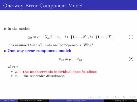
In the model:

yit = α+ X ′itβ + uit i ∈ {1, . . . ,N}, t ∈ {1, . . . ,T} (1)

it is assumed that all units are homogeneous. Why?One-way error component model:

ui,t = µi + εi,t (2)

where:I µi – the unobservable individual-specific effect;I εi,t – the remainder disturbance.


Fixed effects model

We can relax assumption that all individuals have the same coefficients

yit = αi + β1x1it + . . .+ βkxkit + uit (3)

where uit ∼ N (0, σ2u).

Note that an i subscript is added to only intercept αi but the slope coefficients,β1, . . ., βk are constant for all individuals.An individual intercept (αi) are include to control for individual-specificand time-invariant characteristics. That intercepts are called fixedeffects.Independent variables (x1it . . . xkit) cannot be time invariant.Fixed effects capture the individual heterogeneity.The estimation:i) The least squares dummy variable estimatorii) The fixed effects estimator


The Least Squares Dummy Variable Estimator

The natural way to estimate fixed effect for all individuals is to include anindicator variable. For example, for the first unit:

D1i ={

1 i = 10 otherwise (4)

The number of dummy variables equals N . It’s not feasible to use theleast square dummy variable estimator when N is largeWe might rewrite the fixed regression as follows:

yit =N∑

j=1αiDji + β1x1it + . . .+ βkxkit + ui,t (5)

Why α is missing?



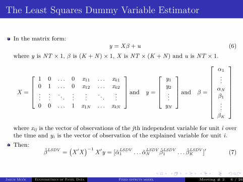
In the matrix form:y = Xβ + u (6)

where y is NT × 1, β is (K + N )× 1, X is NT × (K + N ) and u is NT × 1.

X =

1 0 . . . 0 x11 . . . xk10 1 . . . 0 x12 . . . xk2...

.... . .

......

. . ....

0 0 . . . 1 x1N . . . xkN

and y =

y1y2...

yN

and β =

α1...αNβ1...βK

where xij is the vector of observations of the jth independent variable for unit i overthe time and yi is the vector of observation of the explained variable for unit i.Then:

βLSDV =(X ′X

)−1 X ′y = [αLSDV1 . . . αLSDV

N βLSDV1 . . . βLSDV

K ]′ (7)



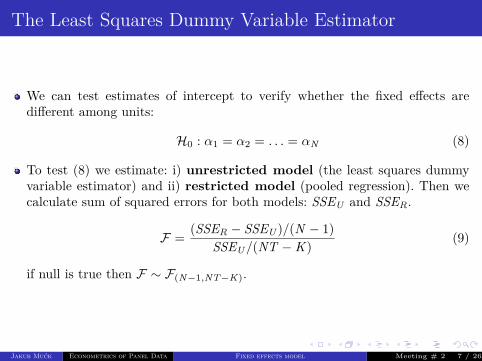
We can test estimates of intercept to verify whether the fixed effects aredifferent among units:

H0 : α1 = α2 = . . . = αN (8)

To test (8) we estimate: i) unrestricted model (the least squares dummyvariable estimator) and ii) restricted model (pooled regression). Then wecalculate sum of squared errors for both models: SSEU and SSER.

F = (SSER − SSEU )/(N − 1)SSEU/(NT −K ) (9)

if null is true then F ∼ F(N−1,NT−K).


The Fixed Effect (Within Group) Estimator

Let’s start with simple fixed effects specification for individual i:

yit = αi + β1x1it + . . .+ βkxkit + uit t = 1, . . . ,T (10)

Average the observation across time and using the assumption on time-invariantparameters we get:

yi = αi + β1x1i + . . .+ βk xki + ui (11)

where yi = 1T∑T

t=1 yit , x1i = 1T∑T

t=1 x1it , xki = 1T∑T

t=1 xkit and ui = 1T∑T

t=1 ui

Now we substract (11) from (10)

(yit − yi) = (αi − αi)︸︷︷︸=0

+ β1(x1it − x1i) + . . .+ βk(xitk − xki) + (uit − ui) (12)

Using notation: yit = (yit − yi), x1it = (x1it − x1i), xkit = (xkit − xki) uit = (uit − ui),we get

yit = β1x1t + . . .+ βk xkt + ui,t (13)Note that we don’t estimate directly fixed effects.


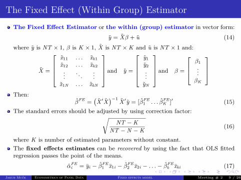
The Fixed Effect (Within Group) EstimatorThe Fixed Effect Estimator or the within (group) estimator in vector form:

y = Xβ + u (14)where y is NT × 1, β is K × 1, X is NT ×K and u is NT × 1 and:

X =

x11 . . . xk1x12 . . . xk2...

. . ....

x1N . . . xkN

and y =

y1y2...

yN

and β =

β1...βK

Then:

βFE =(X ′X

)−1 X ′y = [βFE1 . . . βFE

K ]′ (15)The standard errors should be adjusted by using correction factor:√

NT −KNT −N −K (16)

where K is number of estimated parameters without constant.The fixed effects estimates can be recovered by using the fact that OLS fittedregression passes the point of the means.

αFEi = yi − βFE

1 x1i − βFE2 x2i − . . .− βFE

k xki (17)


Empirical example

Grunfeld’s (1956) investment model:

Iit = α+ β1Kit + β2Fit + uit (18)

whereIit – the gross investment for firm i in year t;Kit – the real value of the capital stocked owned by firm i;Fit – is the real value of the firm (shares outstanding).

The dataset consists of 10 large US manufacturing firms over 20 years(1935–54).


Empirical example

Pooled OLS FEα −42.714 −58.744

(9.512) (12.454)[0.000] [0.000]

β1 0.231 0.310(0.025) (0.017)[0.000] [0.000]

β2 0.116 0.110(0.006) (0.012)[0.000] [0.000]

Note: The expressions in round and squared brackets stand for standard errors andprobability values corresponding to the null about parameter’s insignificance, respectively.

Iit = α+ β1Kit + β2Fit + uit


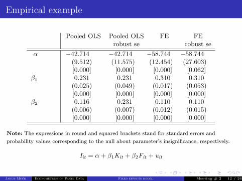
Empirical example

Pooled OLS Pooled OLS FE FErobust se robust se

α −42.714 −42.714 −58.744 −58.744(9.512) (11.575) (12.454) (27.603)[0.000] [0.000] [0.000] [0.062]

β1 0.231 0.231 0.310 0.310(0.025) (0.049) (0.017) (0.053)[0.000] [0.000] [0.000] [0.000]

β2 0.116 0.231 0.110 0.110(0.006) (0.007) (0.012) (0.015)[0.000] [0.000] [0.000] [0.000]




Outline




Jakub Mućk Econometrics of Panel Data Random Effect model Meeting # 2 13 / 26

Random Effect model

Let’s assume the following model

yit = α+ X ′itβ + uit , i ∈ {1, . . . ,N}, t ∈ {1, . . . ,T}. (19)

The error component (ut) is the sum of the individual specific random com-ponent (µi) and idiosyncratic disturbance (εi,t):

uit = µi + εit , (20)

where µi ∼ N (0, σ2µ);

and εi,t ∼ N (0, σ2ε).

Note that independent variables can be time invariant.Individual (random) effects are independent:

E (µi , µj) = 0 ifi 6= j. (21)

Estimation method: GLS (generalized least squares).


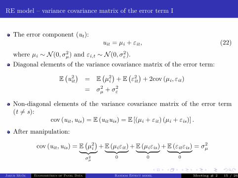
RE model – variance covariance matrix of the error term I

The error component (ut):uit = µi + εit , (22)

where µi ∼ N (0, σ2µ) and εi,t ∼ N (0, σ2

ε).Diagonal elements of the variance covariance matrix of the error term:

E(u2

it)

= E(µ2

i)

+ E(ε2

it)

+ 2cov (µi , εit)= σ2

µ + σ2ε

Non-diagonal elements of the variance covariance matrix of the error term(t 6= s):

cov (uit , uis) = E (uituis) = E [(µi + εit) (µi + εis)] .

After manipulation:

cov (uit , uis) = E(µ2

i)︸︷︷︸

σ2µ

+E (µiεit)︸︷︷︸0

+E (µiεis)︸︷︷︸0

+E (εitεis)︸︷︷︸0

= σ2µ


RE model – variance covariance matrix of the error term II

Finally, variance covariance matrix of the error term for given individual (i):

E (ui.u′i.) = Σu,i =(σ2µ + σ2

ε

)

1 ρ . . . ρ

ρ 1... ρ

......

. . ....

ρ ρ . . . 1

, (23)

whereρ =

σ2µ

σ2µ + σ2

ε

.

Note that Σu is block diagonal with equicorrelated diagonal elements Σu,ibut not spherical.Although disturbances from different (cross-sectional) units are independentpresence of the time invariant random effects (µi) leads to equi-correlationsamong regression errors belonging to the same (cross-sectional) unit.


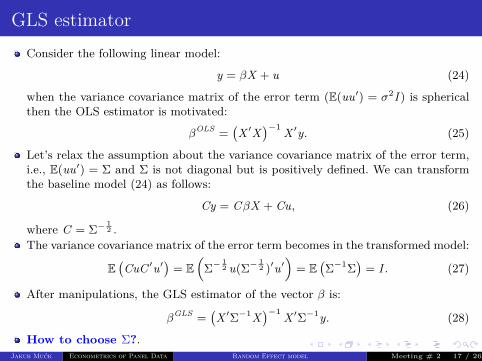
GLS estimatorConsider the following linear model:

y = βX + u (24)

when the variance covariance matrix of the error term (E(uu′) = σ2I ) is sphericalthen the OLS estimator is motivated:

βOLS =(X ′X

)−1 X ′y. (25)

Let’s relax the assumption about the variance covariance matrix of the error term,i.e., E(uu′) = Σ and Σ is not diagonal but is positively defined. We can transformthe baseline model (24) as follows:

Cy = CβX + Cu, (26)

where C = Σ− 12 .

The variance covariance matrix of the error term becomes in the transformed model:

E(CuC ′u′

)= E

(Σ−

12 u(Σ−

12 )′u′

)= E

(Σ−1Σ

)= I . (27)

After manipulations, the GLS estimator of the vector β is:

βGLS =(X ′Σ−1X

)−1 X ′Σ−1y. (28)

How to choose Σ?.Jakub Mućk Econometrics of Panel Data Random Effect model Meeting # 2 17 / 26

Model estimation: RE

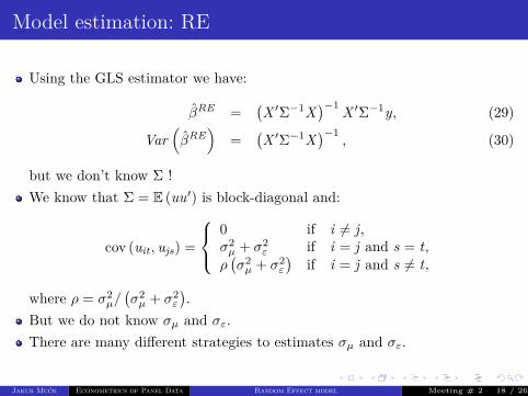
Using the GLS estimator we have:

βRE =(X ′Σ−1X

)−1 X ′Σ−1y, (29)

Var(βRE

)=

(X ′Σ−1X

)−1, (30)

but we don’t know Σ !We know that Σ = E (uu′) is block-diagonal and:

cov (uit , ujs) =

0 if i 6= j,σ2µ + σ2

ε if i = j and s = t,ρ(σ2µ + σ2

ε

)if i = j and s 6= t,

where ρ = σ2µ/(σ2µ + σ2

ε

).

But we do not know σµ and σε.There are many different strategies to estimates σµ and σε.


Model estimation: RE – example

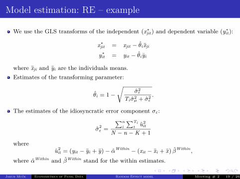
We use the GLS transforms of the independent (x∗jit) and dependent variable (y∗it):

x∗jit = xjit − θi xji

y∗it = yit − θi yi

where xji and yi are the individuals means.Estimates of the transforming parameter:

θi = 1−√

σ2ε

Ti σ2µ + σ2

ε.

The estimates of the idiosyncratic error component σε:

σ2ε =

∑ni

∑Tit u2

it

N − n −K + 1

whereu2

it = (yit − yi + y)− αWithin − (xit − xi + x) βWithin ,

where αWithin and βWithin stand for the within estimates.


Model estimation: RE – example

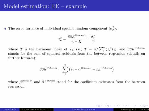
The error variance of individual specific random component (σ2µ):

σ2µ = SSRBetween

n −K − σ2ε

T

where T is the harmonic mean of Ti , i.e., T = n/∑n

i (1/Ti), and SSRBetween

stands for the sum of squared residuals from the between regression (details onfurther lectures):

SSRBetween =n∑i

(yi − αBetween − xi β

Between)where βBetween and αBetween stand for the coefficient estimates from the betweenregression.


Model estimation: RE – Swamy-Arora method

Method which gives more precise estimates in small samples and unbalanced panels.The estimation of σε (the idiosyncratic error component) is the same=⇒ it bases on the residuals from the within regression.

The variance or the individual error term:

σ2µ,SA = SSRBetween − (n −K) σ2

ε

N − tr ,

where SSRBetween is the sum of the squared residuals from the between regressionand

tr = trace{(

X ′PX)−1 X ′ZZ ′X

}P = diag

{ 1Ti

eTi e′Ti

}Z = diag {eTi}

where eTi is a Ti × 1 vector of ones.


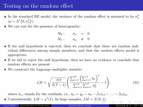
Testing on the random effectIn the standard RE model, the variance of the random effect is assumed to be σ2

µ

(µ ∼ N(0, σ2

µ

)).

We can test for the presence of heterogeneity:

H0 : σµ = 0H1 : σµ 6= 0

If the null hypothesis is rejected, then we conclude that there are random indi-vidual differences among sample members, and that the random effects model isappropriate.If we fail to reject the null hypothesis, then we have no evidence to conclude thatrandom effects are present.We construct the Lagrange multiplier statistic:

LM =√

NT2(T − 1)

(∑Ni=1

(∑Tt=1 uit

)2

∑Ni=1

∑Tt=1 u2

it

− 1

), (31)

where ui,t stands for the residuals, i.e., uit = yit − α0 − β1x1it − . . .− βkxkit .Conventionally, LM ∼ χ2(1). In large samples, LM ∼ N (0, 1).


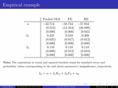
Empirical example

Pooled OLS FE REα −42.714 −58.744 −57.834

(9.512) (12.454) (28.899)[0.000] [0.000] [0.045]

β1 0.231 0.310 0.308(0.025) (0.017) (0.012)[0.000] [0.000] [0.000]

β2 0.116 0.110 0.110(0.006) (0.012) (0.010)[0.000] [0.000] [0.000]




Empirical example

Table: The estimates of the RE model

σµ 84.20σε 52.77ρ 0.72LM 798.16H0 : σµ = 0 [0.000]


Outline




Jakub Mućk Econometrics of Panel Data Comparison of Fixed and Random Effect model Meeting # 2 25 / 26

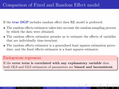
Comparison of Fixed and Random Effect model

If the true DGP includes random effect then RE model is preferred:The random effects estimator takes into account the random sampling processby which the data were obtained.The random effects estimator permits us to estimate the effects of variablesthat are individually time-invariant.The random effects estimator is a generalized least squares estimation proce-dure, and the fixed effects estimator is a least squares estimator.

Endogenous regressorsIf the error term is correlated with any explanatory variable thenboth OLS and GLS estimators of parameters are biased and inconsistent.

Jakub Mućk Econometrics of Panel Data Comparison of Fixed and Random Effect model Meeting # 2 26 / 26

Econometrics of Panel Data - Warsaw School of …web.sgh.waw.pl/~jmuck/EoPD/Meeting2.pdf ·...

Documents

Transcript of Econometrics of Panel Data - Warsaw School of …web.sgh.waw.pl/~jmuck/EoPD/Meeting2.pdf ·...