Econometrics of Energy Markets - Centre de Recherche …€¦ · Students will be trained with the...

Econometrics of Energy MarketsMSc Energy, Finance, Carbon

Université Paris Dauphine

Julien Chevallier∗

December 10, 2010

• Goal:

The objective of this course is to provide students with agood command of time-series tools that may be used for theanalysis of energy markets. The course covers a wide rangeof applications in the oil, natural gas, coal, electricity andCO2 markets. The emphasis is placed on financial economet-rics, through the use of linear regression models, vector au-toregressive models, cointegration models, and GARCH(p,q)models. Students will be trained with the Eviews sofwtarein computer labs in order to replicate research papers in thefield of their choice.

• Pre-requisites: Econometrics I and II.

• Structure: 18 hours course (equivalent to 2.5 ECTS credits) in com-puter rooms, divided in 6 lectures of 3 hours. Practical applicationsunder Eviews software.

• Assessment: 2-hour written exam.

• Eligibility: Students enrolled in the MSc Energy, Finance, Carbon -both in research and professional majors - may register for this course.Students from other MSc need the explicit agreement of the teacherbefore starting the course to be registered. The course is closed tostudents outside of Paris Dauphine University.

∗Paris Dauphine University (CGEMP/LEDa), Place du Marechal de Lattre de Tas-signy, 75775 Paris Cedex 16, France. [email protected]

1

MSc Energy, Finance, Carbon Econometrics of Energy Markets

1 Topic #1: Linear Regression Models

Required reading: Weisberg, S. Applied Linear Regression. Wiley

Series in Probability and Statistics: Chapters #2,3,4,8, 10

1.1 The linear regression model

1.1.1 Presentation

1.1.2 Matrix Notation

1.2 Estimation and Properties of the Estimators

1.2.1 Estimation of regression coefficients

1.2.2 Hypotheses and properties of the estimators

1.2.3 Variance analysis and quality of the adjustment

1.3 Statistical Tests

1.3.1 The role of hypotheses

1.3.2 The construction of tests

1.4 Variance analysis

1.4.1 Variance analysis table and global significance test of the

regression

1.4.2 Other tests in variance analysis

1.5 Use of Dummy Variables

1.5.1 Construction and purpose of dummy variables

1.5.2 Examples

1.6 Forecasting

1.6.1 Conditional forecasting2


1.6.2 Reliability of forecasting and confidence interval

1.7 Multicolinearity and Variables Selection

1.7.1 Partial correlation

1.7.2 Multicolinearity

1.7.3 Selection of explanatory variables

1.8 Model misspecification

1.8.1 Errors autocorrelation

• Problem identification

• Generalized OLS estimator

• Detecting errors autocorrelation

• Estimation procedures in presence of errors autocorrelation

1.8.2 Residuals stability tests

• Rolling regressions

• CUSUM test

1.8.3 Heteroskedasticity

• Problem identification

• Correcting the heteroskedasticity

• Detecting the heteroskedasticity

• Other tests: the ARCH test

3


1.9 Problem Set #1

Download the dataset at the following address:

https://sites.google.com/site/jpchevallier/teaching/data_efc.zip

1.9.1 Qualitative observation of coal, natural gas, and power spot

prices trajectories

Plot the daily spot price trajectories of EEX coal and EEX natural

gas prices.

Comment:

- do you observe spikes (upside peaks followed by downside jumps) in

coal and/or gas prices?

- are the trajectories formed by random oscillations? do the price series

evolve around a random trend?

- does volatility seem higher and spikes more frequent during some spe-

cific periods?

Plot the daily spot price trajectory of Powernext EPEX elec-

tricity prices.

Comment:

- do you observe a seasonal pattern in the power spot price series? is

that different from coal and gas prices?

- can you identify whether downside peaks in power spot price series

correspond to bank holidays?

- are the spikes in power spot prices sharper than those observed in other

price series? if yes, which one(s)?

- are the trajectories of power spot prices mean-reverting (characterized

by random oscillations around a long-term average)?

4


- does volatility seem higher and spikes more frequent during specific

periods?

The seasonality of some commodity spot prices arises from the system-

atic variations of the demand or supply across hours/days/season and from

the impossibility or the difficulty of storing the commodity to absorb these

demand variations.

Mean-reversion in commodity prices can be explained by the following

mechanisms: when prices are high, producers are urged to use their spare

production capacity (inducing short-term reversion in the prices) or to drill

new wells (inducing long-term mean reversion in the prices) and consumers

tend to decrease their consumption e.g. by switching to substitutes, prompt-

ing the prices to go down; when prices are low, producers reduce the quantity

put on the market by stopping or storing production and consumers increase

their consumption e.g. by switching away from substitutes, which prompts

the prices to go up.

1.9.2 Seasonality in Power Prices

Plot the auto-correlations functions of the daily Powernext EPEX

spot price..

- Do you observe correlation peaks following a specific pattern?

- Which prices between day d and day d− n seem more correlated than

prices with other lags?

Before modelling the random part of the spot prices, it is necessary to

filter out the weekly seasonality present in the prices. A simple way of doing

this is to:

- compute the average log price Ld for d = days-of-week.

- substract from these average log prices the global average log price

5


L across all days to obtain an additive seasonality adjustment term Ld =

Ld− L, such that∑n

d=1Ld = 0

- calculate the seasonality adjustment factors πd = exp(Ld) such that

Πnd=1

πd = 1

- divide the prices of the original series by these adjustment factors to

obtain the deseasonalized price series : St =St

πdt

where dt is the week day of

date t

Report the adjustment factors for each day of the week.

- when do you observe that prices are the highest (which day-of week)?

Plots the deseasonalized price series, where you have removed

the bank holidays.

- Do you still observe any systematic patterns (compared to the previous

figure)?

Plot the auto-correlation functions of the two deseasonalized

series.

- Do you still observe regular bumps occurring every interval between

day d and day d− n?

Remark :

- to deseasonalize the hourly spot prices, it is necessary to repeat the above

procedure for each of the 24 hourly time series H1, H2..., H24

- when a yearly seasonality is present, one can perform an Ordinary Least

Square regression of the log prices on sinusoidal functions of period 1 year (in some

situations, 6 months and 3 months seasonal patterns must be added) to obtain

the deseasonalized data ; however, in many situations, the yearly seasonality is not

constant and therefore cannot be well represented by trigonometric series of yearly

seasonality : this phenomenon is due to the variability of weather and storage con-

6


ditions across winters ; in these situations, a wavelet analysis might help decompos-

ing the signal into the sum of a long-term trend, a yearly seasonality with varying

shapes (determined essentially by the strength and the starting/ending dates of the

winter), and a residual noise which will be modeled as a mean-reverting process.

7


2 Topic #2: Basics of Time-Series Econometrics

Required reading: Lutkepohl, H. and Kratzig, M. 2004. Applied

Time Series Econometrics, Cambridge University Press: Chapter

#2.

2.1 Wold’s decomposition theorem

2.2 Lag operator

2.3 ARMA Processes

2.3.1 AR and MA processes

2.3.2 ARMA process

2.4 Stationarity

2.4.1 Definition and properties

2.4.2 Simple and partial autocorrelation functions

2.4.3 White-noise tests

2.5 Problems linked to non-stationarity and unit root tests

2.5.1 DS and TS processes

2.5.2 Unit root tests (ADF, PP, KPSS) and sequential test pro-

cedures

2.6 Chow’s break test

2.6.1 Principle of the test

2.6.2 Sub-samples estimation

8


2.7 Problem Set #2

2.7.1 Stationarity Tests in Power, Coal and Natural Gas Spot

Prices

Statistically, mean-reversion is evidenced by testing the nullity of the coeffi-

cient α in the following regression:

∆xt = xt+1 − xt = αxt + β + et

This test is called the Dickey-Fuller test :

- if α is significantly negative, then we say that the process xt has no

unit root, or that it is stationary, inducing a mean-reverting behavior for the

prices;

- if α is not significantly different from 0, then we say that the process

xt ’has a unit root’, inducing a random walk behavior for the prices.

In practice, Augmented-Dickey-Fuller (ADF) or Phillips-Peron (PP) tests

are used rather than Dickey-Fuller. These tests are based on the same prin-

ciple but corrects for potential serial autocorrelation and time trend in ∆xt

through a more complicated regression :

∆xt =L∑

i=1

βi∆xt−i + αxt + β1t+ β2 + et

The ADF test tests the null hypothesis H0 that č α = 0 (the alternative

hypothesis H1 being that α < 0) by computing the Ordinary Least Squares

(OLS) estimate of α in the previous equation and its t-statistics t; then,

the statistics of the test is the t-statistics tα of coefficient α, which follows

under H0 a known law (studied by Fuller and here denoted Ful). The test

computes the p-value p, which is the probability of Ful ≤ t under H0. If

9


p < 0.05, H0 can be safely rejected and H1 accepted: we conclude that the

series ’xt has no unit root’.

Extensions of these stationarity tests were also developed by Phillips and

Perron (PP, 1988) and Kwiatkowski, Phillips, Schmidt, and Shin (KPSS,

1992).

Report the ADF, PP, and KPSS tests for logarithmic Pow-

ernext electricity, Powernext gas, EEX gas and EEX coal spot

prices.

- What do you conclude? For which time-series can H0 be rejected? For

which time-series can you not reject H0?

- Detail the methodology to transform non-stationary variables to sta-

tionary, and the possible bias induced if the process is TS or DS.

2.7.2 Calibration of Mean-Reversion Models

The simplest mean-reversion model is the so-called AR(1) model:

xt+1 = ρxt + β + et+1

where the (et) are i.i.d with law N(0, σ2).

The calibration proceeds in two steps :

1. the coefficients ρ and β are determined by OLS regression of xt+1 on

xt;

2. σ is computed as the standard deviation of the residuals of the regres-

sion

Calibrate this model to the electricity, coal and gas log spot

prices.

10


The mean-reversion characteristic time is computed as τ = 1

1−ρ. It equals

15 days for electricity, 30 days for coal and gas. We are faced now with four

types of problem using the mean-reversion model :

1. the residuals of the AR(1) model are correlated (test the hypothesis

H0 that the residuals are uncorrelated using the Box-Pierce

test): this could be dealt with by switching to the ADF model;

2. the residuals do not follow a normal distribution (test the hypothesis

H0 that the residuals follow a Gaussian law; this test is called

the Jarque-Bera test). This difficulty could be overcome by:

• replacing the normal distribution by a density presenting fat tails

(e.g. the Normal Inverse Gaussian or Generalized Error Distribu-

tion), but in this case, nothing would guarantee that large posi-

tive jumps will first occur and then be followed by large negative

jumps;

• by introducing the possibility of random positive jumps occurring

at random times (the negative ’jumps’ being generated by the

mean-reversion parameter α = ρ− 1:

xt+1 − xt = αxt + β + et+1 + qt+1Jt+1

where qt+1 is a random variable taking values 1 (jump) or 0 (no

jump) with probabilities p and 1−p and Jt+1 is a positive random

jump; but in this case, the mean-reversion speed α will be too

high to account for mean-reversion in normal periods as it has

to capture the mean-reversion in both normal periods and spike

regimes.

11


3. the residuals present heteroscedasticity: their variance is not constant

in time (test the hypothesis H0 that the squared residuals are

uncorrelated using the Box-Pierce test); this could be overcome

by introducing a GARCH (Generalized Auto Regressive Conditional

Heteroscedasticity) model (see Topic 5).

To visualize these difficulties, plot the graphs testing the relevance

of AR(1) model on electricity, coal and gas log prices.

A second test of relevance for a model (M) is to compare the observed

trajectories with the ones generated by the model (M).

- What do you observe? Which simulated path under the AR(1) model

with normal noise does not look like the observed one (absence of peaks, too

large volatility compared to normal periods, etc.)?

- Which simulated path looks more like the observed path, apart from

the absence of peaks and the non-stochastic and non-seasonal volatility?

Assess the realism of the paths generated by the AR(1) model

(with NIG noise) and the random positive jumps model for coal

natural gas.

Plot the observed and simulated paths under the random pos-

itive jumps model with reasonable choice of parameters.

- What do you observe? Which model produces much more realistic

paths than the simple auto-regressive the AR(1) model?

Note that to produce fast mean-reverting jumps, the parameter α has

to be highly negative, provoking excessive mean-reversion speed in normal

periods.

12


3 Topic #3: Vector AutoRegressive Models

Required reading: Watson, M.W. 1994. Vector autoregressions

and cointegration. Handbook of Econometrics 4, 2843-2915.

3.1 VAR Model Representation

3.1.1 Example

3.1.2 General representation

3.1.3 ARMAX representation

3.2 Parameters estimation

3.2.1 Estimation method

3.2.2 Lag determination

3.2.3 Forecasting

3.3 VAR Dynamics

3.3.1 VMA representation

3.3.2 Shocks analysis: Impulse Response Functions

3.3.3 Variance decomposition

3.4 Causality

3.4.1 Causality in the Granger sense

3.4.2 Causality in the Sims sense

13


3.5 Problem Set #3

Dependence models for stationary commodity prices

The traditional model for correlated stationary prices is the Vector-Auto-

Regressive model (VAR), which is the multi-variate extension of the Auto-

Regressive model.

Let Zt =

X1t

X2t

be the vector process formed of the two (properly

deseasonalized) log prices. Then, the VAR(p) model reads :

Zt = C + Γ1Zt−1 + . . .+ ΓpZt−p + ǫt

where C =

C1

C2

is a constant vector, Γ1, . . . ,Γp are 2x2 matrices and

the vector process ǫt =

ǫ1t

ǫ2t

is formed of independent random variables

following a centered bi-variate normal distribution N(0,∑

).

The calibration of the model VAR(p) proceeds in three classic steps:

1. the optimal order p is selected using an information criterion, which is

an indicator of the relevance of a model, giving a positive weight to the

likelihood of the model and a negative weight to the number of model

parameters ; e.g., the Schwartz Information Criterion (SIC) is equal

to 2LL − ln(T )n, where LL is the log-likelihood, T is the number of

observations and n is the number of parameters of the model.

2. once p is known, C,Γ1, . . . ,Γp are determined by OLS.

3. lastly, the standard deviation and correlation of the residuals give ma-

trix∑

14


Perform the calibration of the VAR model on the pairs Pow-

ernext electricity/gas and EEX gas/coal.

Report the following results:

1. the lag order optimizing the information criteria;

2. the results of the two OLS regressions on lagged prices;

3. the correlation between the electricty and natural gas residuals.

Assess whether the causality runs positively (negatively) from

Powernext electricity (natural gas) to natural gas (electricity), and

explain why with respect to the regression coefficients of electricity

(natural gas) on the lagged natural gas (electricity) prices (sign &

significance).

Repeat the analysis with EEX gas/coal prices.

More generally, we will say that a process P 1t Granger causes P 2

t at the or-

der p if, in the linear regression of P 2t on lagged prices P 1

t−1, . . . , P1t−p, P

2t−1, . . . , P

2t−p,

at least one of the regression coefficients of P 1t on the lagged prices P 2

t−1, . . . , P2t−p

is significantly different from 0. The intuition behind Granger causality is

that the information on past prices P 2t−1, . . . , P

2t−p is relevant to forecast P 1

t

at future time t.

Granger causality is examined using the Granger causality test testing

the null hypothesis H0 that all regression coefficients of P 1t on the lagged

prices P 2t−1, . . . , P

2t−p are null. A p-value lower than 0.05 means that H0 can

be rejected (and causality accepted) with 95% confidence level.

Perform the Granger causality tests on the pairs Powernext

electricity/gas and EEX gas/coal.

How well does the VAR(p) model perform to account for the

spikes observed in the trajectories of previous problem sets?

15


A model capturing correlated jumps between commodity spot prices is

proposed by Benth and Kettler (2006) : the idea consists in describing the

gas and electricity log spot prices by a VAR(1) process with non-Gaussian

correlated residuals modeled by a copula representation.

The idea behind copulas is to disentangle the problems of fitting the

margin distributions and the dependence structure. Typically, the first task

is performed first (using e.g. Normal Inverse Gaussian distribution for each

residual separately), followed by the maximum-likelihood fit of a chosen class

of copula.

Perform IRF analysis based on the most appropriate choice of

decomposition for the pairs Powernext electricity/gas and EEX

gas/coal.

Perform variance decomposition analysis for the pairs Pow-

ernext electricity/gas and EEX gas/coal.

16


4 Topic #4: Cointegration and Error Correction

Models

Required reading: Watson, M.W. 1994. Vector autoregressions

and cointegration. Handbook of Econometrics 4, 2843-2915.

4.1 Examples

4.2 The concept of cointegration

4.2.1 Properties of the order of integration of a time-series

4.2.2 Conditions for cointegration

4.2.3 The Error Correction Model

4.3 Cointegration between 2 variables

4.3.1 Cointegration test between 2 variables: : the Engle-Granger

procedure

4.3.2 Estimation of the Error Correction Model

4.4 Cointegration between k variables

4.4.1 Cointegration test between k variables: the Johansen pro-

cedure

4.4.2 Estimation of the Error Correction Model

4.4.3 Dynamics and Vector Error Correction Models

4.4.4 Cointegration Relation Tests

4.4.5 Summary of the test procedure

17


4.5 Problem Set #4

4.5.1 Dependence models for non-stationary commodity prices

For non-stationary processes, it is impossible to use a VAR(p) model, which

intrinsically applies to mean-reverting time series. Therefore, we use the

concept of cointegration :we look for a stationary linear combination of the

two series, which will represent the long-run equilibrium and we study the

error-correction mechanisms insuring the reversion to the long-run equilib-

rium. For example, when we study the correlation between crude oil and

gasoline, it is reasonable to test whether the crack-spread is mean-reverting

and to expect a correction of an abnormally high/low crack spread via crude

oil or gasoline prices.

Let us apply this idea to the pair of EEX gas/Powernext gas spot prices,

for which you have studied stationarity in Problem Set #2.

Report the results of the OLS regression of EEX gas spot log

prices on Powernext gas spot log prices.

Apply the 3 standard stationarity tests (ADF, PP, KPSS) to

the residuals of the regression.

- which obtain p-value do you obtain for the Augmented-Dickey-Fuller

test and for the Phillips-Perron test?

- can you safely reject the hypothesis of existence of a unit root, hence

conclude to the stationarity of the residuals?

The last step of the cointegration model consists in describing the dy-

namics of the two series in terms of the residuals of the long-term relation:

∆Xet

∆Xe′

t

=

µe

µe′

+∑p

k=1Γk

∆Xet−k

∆Xe′

t−k

+

Πe

Πe′

Rt+

ǫet

ǫe′

t

where

• e stands for EEX gas, and e′ stands for Powernext gas;

18


• Xet is the log spot price of energy e at time t;

• the 2x1 vector process ∆Zt =(

∆Xet = Xe

t+1 −Xet ,∆Xe′

t = Xe′

t+1 −Xe′

t

)

′

is the vector of EEX gas and Powernext gas price returns;

• µ = (µX,e, µX,e′) is the 1x2 vector composed of the constant part of

the drifts;

• Γk are 2x2 matrices expressing dependence on lagged returns;

• (Rt = Xet − βXe′

t ) is the process composed of the deviations to the

long-term relation between the EEX gas and Powernext gas log spot

prices;

• Π is a 2x1 vector matrix expressing sensitivity to the deviations to the

long-term relation between the EEX gas and Powernext gas prices;

• the residual shocks (ǫet , ǫe′

t ) are assumed to be i.i.d with a centered

bi-variate normal distribution N(0,∑

).

Calibrate the model by following the following steps:

1. check, using unit root tests, that the log prices of EEX gas and Pow-

ernext gas are non stationary and integrated of order one: this amounts

to checking that they are difference stationary, i.e. ∆Xet and ∆Xe′

t are

stationary;

2. check that they are cointegrated, i.e. β exists such that Rt = Xet −βXe′

t

is stationary. This can be done by performing an OLS regression of Xet

on Xe′

t or more rigorously by using the Johansen cointegration test;

3. then, the optimal lag p is selected using an information criterion;

19


4. compute Γ and Π by OLS regression of the returns on lagged returns

and past deviation (Rt).

5. the standard deviation and correlation of the residuals (ǫet , ǫe′

t ) give

matrix∑

- concerning step #4: do you observe that either EEX gas or Powernext

gas returns correct the deviations to the long-term equilibrium?

- can you conclude that EEX gas or Powernext gas is the leader in the

long-term price discovery?

- can you identify a positive causality runs from EEX gas returns to

Powernext gas returns (or conversely)?

- do you should observe that EEX gas price evolution is completely in-

dependent of Powernext gas prices?

4.5.2 VECM Analysis

We want to introduce an error-correction mechanism on the levels and on

the slopes between the energies e and e′.

Let Xt be a vector of N variables, all I(1):

Xt = Φ1Xt−1 + . . . +ΦpXt−p + ǫt

with ǫt ∼ WGN(0,Ω), WGN denotes the White Gaussian Noise, Ω

denotes the variance covariance matrix, and Φi (i = 1, . . . , p) are parameter

matrices of size (NxN).

Under the null H0, there exists r cointegration relationships between N

variables, i.e. Xt is cointegrated with rank r.

The error correction model writes:

20


∆Xt = Π1∆Xt−1 + . . .+Πp−1∆Xt−p+1 +ΠpXt−p + ǫt

where the matrices Πi (i = 1, . . . , p) are of size (NxN).

All variables are I(0), except Xt−p which is I(1).

For all variables to be I(0), ΠpXt−p needs to be I(0) as well.

Let Πp = −βα′, where α′ is an (r,N) matrix which contains r cointegra-

tion vectors, and β is an (N, r) matrix which contains the weights associated

with each vector.

If there exists r cointegration relationships, then Rk(Πp) = r. Johansen’s

cointegration tests are based on this condition.

∆Xt = Π1∆Xt−1 + . . .+Πp−1∆Xt−p+1 − βα′Xt−p + ǫt

Estimate the VECM through maximum likelihood methods.

Compute the trace test statistics and maximum eigenvalue test

statistics associated with Johansen’s methodology.

Plot two examples of simulated price paths under the VECM

model.

- What do you observe from these two graphs?

- Does the VECM model generate drastically different long-term price

behaviors?

When evaluating the risk of multi-commodity spot exposures, it is im-

portant to filter out the economically non-plausible paths. It is therefore

crucial to complement a statistical model with some economic insights giv-

ing e.g. some deterministic reasonable bounds for gas and coal prices in

the long-term. Then, a constrained VECM model can be simulated with

reflecting upside and downside (possibly time-dependent but deterministic)

21


barriers representing the economic upper and lower bounds for commodity

prices in the long-term.

22


5 Topic #5: GARCH(p,q) Models

Required reading: Bollerslev, B., Engle, R.F., Nelson, D.B. 1994.

ARCH models. Handbook of Econometrics 4, 2959-3038.

5.1 General presentation and problem identification

5.2 ARCH models

5.2.1 Model specifications

5.2.2 Properties of the ARCH(1) model

5.3 ARCH Model tests

5.4 Estimation method and forecasting

5.5 GARCH Processes

5.5.1 Model specification

5.5.2 Test and estimation method of GARCH models

5.6 Other GARCH models

5.6.1 ARCH-in-mean

5.6.2 EGARCH

5.6.3 TGARCH

5.6.4 IGARCH

23


5.7 Problem Set #5

Download BlueNext CO2 spot prices for Phase II at the following address:

https://sites.google.com/site/jpchevallier/teaching/data_efc.zip

5.7.1 Calibrating GARCH models for carbon prices

Pre-estimation

Examine the descriptive statistics for CO2 price series: how well

do they seem to fit GARCH(p, q) models specifications?

Examine the plots of autocorrelation, partial autocorrelation,

and autocorrelation of squared logreturns for the CO2 price series.

You should observe:

• Little serial correlation in the raw returns (P-value of the Ljung-Box

test at the 5% level).

• Significant serial correlation in the squared returns (P-value of the

Ljung-Box test at the 5% level).

• Evidence of heteroskedasticity (ARCH test at the 5% level).

GARCH(p, q) estimation

1. Using the Box-Jenkins methodology, configure the ARMA(p, q)

processes that provide the best fit to the CO2 time-series.

2. Estimate the corresponding GARCH(p, q) model for the CO2

price series.

Yt = θX ′

t + ǫt

24


σ2t = ω +

p∑

i=1

αiǫ2t−i +

q∑

j=1

βjσ2t−j

with σ2t the conditional variance, which is function of a constant term

ω, the ARCH term ǫ2t−i, and the GARCH term σ2t−j .

Comment on:

• the statistical significance of the parameters obtained in the mean and

variance equations;

• the sensitivity of the results obtained to the estimation methodology

(usually QML and BHHH);

• the value of the Ljung-Box test;

• the value of the ARCH test;

• the plot of autocorrelation of squared logreturns for the CO2 price

series;

• the innovations, conditional standard deviations, and standardized in-

novations of the GARCH (p, q) model.

You should observe:

• No correlation.

• Little volatility clustering. Modeling similar to Benz and Truck (2009).

• Including a dummy variable for the structural break from April 25 to

June 23, 2006 is not significant.

Other GARCH(p, q) models

25


Consider other models than the standard GARCH(p, q) model with a

Gaussian conditional probability distribution.

Let us recall the specification for the conditional variance proposed by

Nelson (1991):

log(σ2t ) = ω +

p∑

i=1

αi

∣

∣

∣

∣

ǫt−i

σt−i

∣

∣

∣

∣

+

q∑

j=1

βj log(σ2t−j) +

r∑

k=1

γkǫt−k

σt−k

where γ tests for the presence of the leverage effect1.

The PARCH specification allows to model the standard deviation rather

than the variance, and may be written as follows (Ding et al. (1993)):

σδt = ω +

p∑

i=1

αi(|ǫt−i| − γiǫt−i)δ +

q∑

j=1

βjσδt−j

with δ > 0, |γi| ≤ 1 ∀i = 1, . . . , τ , γi = 0 ∀i > τ , τ < p. δ is the

power parameter of the standard deviation, and γ parameters to capture

asymmetry up to order τ .

Finally, the asymmetric TGARCH model by Zakoian (1994) may be writ-

ten as:

σ2t = ω +

p∑

i=1

αiǫ2t−i +

q∑

j=1

βjσ2t−j +

r∑

k=1

γkǫ2t−kΓt−k

where Γt = 1 if ǫt < 0, and 0 otherwise. ǫt−i > 0 and ǫt−i < 0 denote,

respectively, good and bad news.

Do you observe any improvement with GJR-GARCH, EGARCH,

PARCH or alternative specification structures in the variance equa-

tion based on likelihood ratio tests, AIC and BIC?

1Recall that the leverage effect implies a higher level of volatility associated to decreas-ing prices in the financial economics literature.

26


5.7.2 Multivariate analysis

Include other energy variables in your analysis (e.g., coal, gas, . . . ).

Compute the matrix of cross-correlations between energy vari-

ables: can you detect some problematic multicollinearities?

Report the GARCH(p, q) estimates for the CO2 with coal and/or

natural gas regressors.

Which variables are significant? Drop non-significant variable

to obtain your reduced form model.

How can you interpret the sign of the coefficients obtained?

Provide the plot of autocorrelation of squared logreturns, innovations,

conditional standard deviations and standardized innovations, along with

usual diagnostic tests.

27


6 Textbooks

• Hamilton, J.D. 1996. Time Series Analysis, Princeton University Press.

• Lutkepohl, H. and Kratzig, M. 2004. Applied Time Series Economet-

rics, Cambridge University Press.

• Vogelvang, B. 2005. Econometrics: Theory & Applications With Eviews,

Pearson Education Limited.

• Weisberg, S. Applied Linear Regression. Wiley Series in Probability

and Statistics.

28


7 Past Exams (2009-2010)

1) Consider the time-series in Figure 1:

• Briefly describe the variables that you observe, as well as their be-

haviour. What are the differences between the two panels? (1 pt)

MAR07 JUL07 DEC07 MAY08 SEP08 FEB09−10

−5

0

5

10

15

20

25

30

Pric

e in

EU

R/to

n of

CO

2

EUACERSPREAD

0 100 200 300 400 500 6002

2.5

3

3.5

Figure 1: Raw time-series (top panel) and natural logarithms (bottom panel)of the ECX EUA December 2008/2009 Futures and Reuters CER Price Indexfrom March 9, 2007 to March 31, 2009

29


2) Consider the descriptive statistics in Table 1:

• Briefly comment on the descriptive statistics that you observe for each

variable (1 pt)

Variable Mean Median Max Min Std.Dev.

Skew. Kurt.

Raw Price Series

EUA 20.40389 21.52000 29.33000 8.20000 4.459218 -0.765966 3.031938CER 15.85798 16.06875 22.8500 7.484615 2.986495 -0.351494 3.135252

Natural Logarithms

EUA 2.986643 3.068983 3.378611 2.104134 0.255164 -1.323179 4.275898CER 2.743941 2.776876 3.128951 2.012850 0.205511 -0.994736 4.182189

Table 1: Summary Statistics for the Raw Time Series and Natural Loga-rithms

Note: EUA refers to ECX EUA December 2008/2009 Futures, and CER toReuters CER Price Index. Std.Dev. stands for Standard Deviation, Skew.for Skewness, and Kurt. for Kurtosis. The number of observations is 529.

30


In what follows, the ECX EUA December 2008/2009 and Reuters CER

Price Index Raw Series are expressed in natural logarithms.

3) Comment on Tables 2 and 3:

• Which cointegration space can you identify, given a 5% significance

level? Provide detailed comments as to which statistics you use, and

how you read Tables 2 and 3. (2 pts)

Hypothesis Statistic 10% 5% 1%

r ≤ 1 1.65 6.50 8.18 11.65r=0 6.81 12.91 14.90 19.19

Table 2: Cointegration Rank: Maximum Eigenvalue Statistic

Hypothesis Statistic 10% 5% 1%

r ≤ 1 1.65 6.50 8.18 11.65r=0 8.46 15.66 17.95 23.52

Table 3: Cointegration Rank: Trace Statistic

31


4) Comment on Tables 4 to 6:

• Based on your conclusion in Question #3, interpret the following Error

Correction Model. (2 pts)

Variable EUA(1) CER(1)

EUA(1) 1.0000 1.0000CER(1) -1.291699 0.2616575

Table 4: Cointegration Vector

Note: EUA refers to ECX EUA December 2008/2009 Futures, and CER

to Reuters CER Price Index, transformed to natural logarithms. Lag orderin parenthesis. The number of observations is 529.

Variable EUA(1) CER(1)

EUA.d 0.01979082 -0.003906266CER.d 0.02820092 -0.001641289

Table 5: Model Weights


to Reuters CER Price Index, transformed to natural logarithms. Lag orderin parenthesis. .d refers to difference. The number of observations is 529.

Variable EUA.d CER.d

Error Correction Term

ect -0.0197908 -0.0282009

Deterministic

constant 0.0106349 0.0154190

Lagged differences

EUA.d(1) -0.0641515 -0.0504123CER.d(1) 0.2307197 0.1423340

Table 6: VECM with r = 1


to Reuters CER Price Index, transformed to natural logarithms. Lag orderin parenthesis. .d refers to difference. ect refers to the Error CorrectionTerm. The number of observations is 529.

32


In what follows, the ECX EUA December 2008/2009 and Reuters CER

Price Index Raw Series are expressed in log-returns.


• Briefly describe the variables that you observe, as well as their be-

haviour. What are the differences compared to Figure 1? (1 pt)

MAR07 JUL07 DEC07 MAY08 SEP08 FEB09−0.2

−0.15

−0.1

−0.05

0

0.05

0.1

0.15

EUACER

Figure 2: Raw time-series (left panel) and logreturns (right panel) of theECX EUA December 2008/2009 Futures and Reuters CER Price Index fromMarch 9, 2007 to March 31, 2009

33


6) Consider the descriptive statistics in Table 7:

• Briefly comment on the descriptive statistics that you observe for each

variable (1 pt)

Variable Mean Median Max Min Std.Dev.

Skew. Kurt.

Log-Returns

EUA -0.000437 0.0001 0.113659 -0.094346 0.026833 -0.060828 4.868026CER -0.000309 0.0001 0.112545 -0.110409 0.024441 -0.370323 5.961950

Table 7: Summary Statistics for the Log-Returns

Note: EUA refers to ECX EUA December 2008/2009 Futures, and CER toReuters CER Price Index. Std.Dev. stands for Standard Deviation, Skew.for Skewness, and Kurt. for Kurtosis. The number of observations is 529.

34


You are given the following information:

• Optimal lag selection: AIC(n)=4, HQ(n)=1, SC(n)=1, FPE(n)=4.

• p-value of the Portmanteau test < 5% for VAR(1) residuals.

7) Comment on Tables 8 and 9:

• Provide detailed comments of the static VAR analysis for both vari-

ables. (3 pts)

Variable Estimate Std. Er-ror

t-value Pr(>| t |)

Lagged levels

EUA(1) -0.06061 0.08233 -0.736 0.46193CER(1) 0.2454*** 0.08952 2.741 0.00634EUA(2) -0.1504* 0.08227 -1.828 0.06806CER(2) 0.01805 0.08981 0.201 0.84082EUA(3) -0.1275 0.08234 -1.549 0.12198CER(3) 0.2056** 0.08992 2.287 0.02261EUA(4) 0.152601* 0.08203 1.860 0.06342CER(4) -0.07958 -0.09050 -0.879 0.37965Deterministic

const. 0.003480 0.002344 1.484 0.13831trend -0.000015** 0.000008 -1.912 0.05646

ResidualsStd.Error

0.02613

R-Squared 0.07136AdjustedR-Squared

0.0551

F-Statistic 0.00001

Table 8: VAR(4) Model Results for the EUA Variable


to Reuters CER Price Index. Lag order in parenthesis. Std.Error standsfor Standard Error, const. for deterministic constant, and trend fordeterministic trend. p-value is given for the F-Statistic. *** denotes 1%, **5%, and * 1% significance levels. The number of observations is 529.

35


Variable Estimate Std.Error

t-value Pr(>| t |)

Lagged levels

EUA(1) -0.05705 0.07546 -0.756 0.44995CER(1) 0.1627** 0.08206 1.983 0.04787EUA(2) -0.08439 0.07541 -1.119 0.26360CER(2) -0.01538 0.08232 -0.187 0.85188EUA(3) -0.1937*** 0.07547 -2.566 0.01056CER(3) 0.2476*** 0.08242 3.004 0.00279EUA(4) 0.1201 0.07519 1.597 0.11079CER(4) 0.001684 0.08296 0.020 0.98381Deterministic

const. 0.002553 0.002149 1.188 0.23532trend -0.00001 0.000007 -1.517 0.12979

ResidualsStd.Error

0.02395

R-Squared 0.06089AdjustedR-Squared

0.04445

F-Statistic 0.00016

Table 9: VAR(4) Model Results for the CER Variable


to Reuters CER Price Index. Lag order in parenthesis. Std.Error standsfor Standard Error, const. for deterministic constant, and trend fordeterministic trend. The number of observations is 529.

36


8) Comment on Table 10:

• Analyze the diagnostic tests for the VAR(4) model. Can you conclude

that the model is well-specified? (1 pt)

Test Statistic D.F. p-value

Portmanteau 57.4878 48 0.16ARCH VAR 97.1946 9 0.01JB VAR 147.6817 4 0.01Kurtosis 143.5005 2 0.01Skewness 4.1811 2 0.1236

Table 10: Diagnostic tests of VAR(4) Model

Note: Portmanteau is the asymptotic Portmanteau test with a maximumlag of 16, ARCH VAR is the multivariate ARCH test with a maximum lagof order 5, JB is the Jarque Berra normality test for multivariate seriesapplied to the residuals of the VAR(4), Kurtosis and Skewness are separatetests for multivariate skewness and kurtosis.

37



• What can you conclude concerning the Granger causality tests? (1 pt)

Test Statistic p-value

Cause=CER

Granger 3.2237 0.01215Instant 218.49 0.0001

Cause=EUA

Granger 2.7535 0.02695Instant 218.49 0.0001

Table 11: Granger Causality Tests

38



• Briefly comment on the impulse response functions that you observe

for each variable (2 pts)

• Given your analysis in Questions #3 to #9, which decomposition order

has been chosen to compute these graphs? (1 pt)

2 4 6 8 10

−0.

20−

0.15

−0.

10−

0.05

0.00

0.05

0.10

cer

Impulse Response from eua

2 4 6 8 10

0.00

00.

001

0.00

20.

003

0.00

40.

005

0.00

6

eua

Orthogonal Impulse Response from cer (cumulative)

Figure 3: Impulse responses from EUA to CER (top panel) and from CERto EUA (bottom panel) Variables of the VAR(4) Model

39


In what follows, the GARCH(p,q) model with a Gaussian conditional

probability distribution has been estimated by Quasi-Maximum Likelihood

with the BHHH algorithm.


• Provide detailed comments for each parameter of the GARCH(p,q)

model. (2 pts)

Mean Equation

α -0.0002(0.0006)

Variance Equation

κ 0.0002***(0.0000)

β 0.1110(0.1207)

φ 0.3194***(0.0504)

Diagnostic Tests

Ljung-Box 0.9631ARCH test 0.9687Log-Likelihood 1331.7AIC -2619.3BIC -2602.8

Table 12: GARCH estimates for the CER-EUA Spread

Note: The values reported in parentheses are the standard errors. ***indicates 1% level significance, ** 5% level significance, and * 1% levelsignificance. The model estimated is:

spread = α+ ǫt

σ2t = κ+ βσ2

t−1 + φǫ2t−1

40



• What can you conclude with respect to the autocorrelation structure

of GARCH estimates? (1 pt)

0 5 10 15 20−0.2

0

0.2

0.4

0.6

0.8

Lag

Sam

ple

Aut

ocor

rela

tion

Sample Autocorrelation Function (ACF)

Figure 4: GARCH(1,1) model autocorrelation of squared logreturns of theCER-EUA Spread

41



• As a diagnostic check of these estimates, what can you conclude from

Figure 5? (1 pt)

MAR07 MAY07 JUL07 OCT07 DEC07 FEB08 MAY08 JUL08 SEP08 DEC08−0.1

0

0.1Innovations

Inno

vatio

n

MAR07 MAY07 JUL07 OCT07 DEC07 FEB08 MAY08 JUL08 SEP08 DEC080

0.02

0.04

0.06Conditional Standard Deviations

Sta

ndar

d D

evia

tion

MAR07 MAY07 JUL07 OCT07 DEC07 FEB08 MAY08 JUL08 SEP08 DEC08−5

0

5

Inno

vatio

n

Standardized Innovations

CER−EUA 08

Figure 5: GARCH(1,1) model of the CER-EUA Spread innovations (toppanel), conditional standard deviations (middle panel) and standardized in-novations (bottom panel)

42

Econometrics of Energy MarketsMSc Energy, Finance, Carbon

Université Paris Dauphine, Spring 2011

Julien Chevallier∗, Yannick Le Pen†

January 21, 2011

2 hours. No documents allowed. No calculator allowed.

Exam

∗Université Paris Dauphine (CGEMP/LEDa), Place du Maréchal de Lattre de Tassigny,75775 Paris Cedex 16, France. [email protected]

†Université Paris Dauphine (CGEMP/LEDa), Place du Maréchal de Lattre de Tassigny,75775 Paris Cedex 16, France. [email protected]

1


1 Exercise #1 (5 points)

In ‘Crude Oil Volatility: Hedgers or Investors’ (Economics Bulletin 30(4),2877-2883), Milunovich and Ripple (2010) evaluate differential effects of thetrading activity of two classes of traders: hedgers and general investors, onthe volatility of the NYMEX crude oil futures returns.

They select 4 variables:

1. the Standard & Poor’s 500 stock market index (S&P500);

2. Morgan Stanley Capital International (MSCI) US Government long-term bond index;

3. NYMEX Light Sweet Crude Oil Futures Prices;

4. West Texas Intermediate (WTI) Crude Oil Spot Prices.

1) Comment the descriptive statistics in Figure 1 (1 point):

Figure 1: Summary Statistics - weekly returns (%)

2


The authors estimate the conditional variance for crude oil futures returnseries based on Nelson’s (1991) EGARCH model:

ln(σ2

f,t) = ω + α

∣

∣

∣

∣

uf,t−1

σf,t−1

∣

∣

∣

∣

+ βuf,t−1

σf,t−1

+ γ(ht−1 −H)2 + δ(wf,t−1 −W f )2 (1)

where:

• The log of the conditional variance equation ln(σ2f,t) for the oil futures

return is specified as an EGARCH process with two additional volatilityspillovers terms (ht−1 −H)2 and (wf,t−1 −W f )

2.

• (ht−1−H)2 is the squared deviation of the conditional hedge ratio ht−1

from its unconditional value H, and acts as a measure of the conditionalhedge ratio volatility. A positive (negative) and statistically significantγ coefficient would indicate that the rebalancing of hedged positions inone period increases (decreases) oil futures price volatility in the nextperiod.

• (wf,t−1 − W f )2 is a proxy for the volatility of the optimal portfolio

crude oil futures weight wf,t−1. Statistical significance and sign of thecoefficient δ are interpreted in the same manner as for γ.

• The optimal hedge ratio ht and the portfolio weights wt are computedusing standard mean-variance optimization formulas1.

• The variableuf,t−1

σf,t−1

is the standardized oil futures return and controls

for an asymmetric response in the conditional volatility.

1A single horizon mean-variance investor chooses the tangency portfolio that has the

following vector of weights: wt =

∑−1

t µ

i′∑−1

t µ, where

∑

is the unconditional covariance

matrix. The optimal hedge ratio is given by ht =σf,s,t

σ2

f,t

. µ is a 4 × 1 vector of excess

expected returns set equal to their historical averages, while i is a 4× 1 vector of ones.

3


2) Comment the resulting coefficient estimates of the crude oilconditional volatility reported in Figure 2 (2 points):

Figure 2: Crude oil conditional volatility from the EGARCH model

The model implies that, when hedgers and investors set out to incorporatea futures contract into a hedging or investment portfolio strategy, they willbegin with some benchmark for the level of inclusion2. Having established abenchmark, market participants will then monitor the market and rebalanceto maintain an optimal position.

A natural relationship to monitor is the deviation between the uncondi-tional (benchmark) values and their time-varying conditional counterparts:

• when a re-estimated time varying optimal conditional hedge ratio devi-ates from the benchmark, the hedger will have an incentive to rebalancethe hedged position;

• similarly, this is the case for the investor with respect to the optimalportfolio weight.

The rebalancing induces trading activity, and the more volatile is the de-viation between the benchmark and the optimal conditional measure, themore we expect trading activity to increase and to influence the volatility ofreturns.

2Within this framework, the benchmarks are the optimal unconditional hedge ratio andthe optimal unconditional portfolio weight for crude oil.

4


3) Interpret the results obtained in Figures 3 and 4 (2 points):

Figure 3: Estimated conditional crude oil futures hedge ratio

Note: Conditional confidence interval bounds are calculated as ht ± 2√

(ht −H)2.

Figure 4: Estimated conditional crude oil futures portfolio weightNote: Conditional confidence interval bounds are calculated as wf,t ±

2√

(wf,t −W f )2.

5


2 Exercise #2 (5 points)

In ‘The role of market fundamentals and speculation in recent price changesfor crude oil’ (Energy Policy 39, 105-115), Kaufmann (2011) examines howrecent changes in crude oil future prices may be related to market fundamen-tals and/or speculative pressures (by ‘noise traders’).

The author examines the causal relationships among the following vari-ables:

• a monthly measure of dry cargo bulk freight rates (SHIP3 measured inlogs);

• the refiner’s acquisition cost of foreign oil;

• the US average landed price of crude oil from non-OPEC nations;

• the US average landed price of crude oil from OPEC nations;

• the average fob price for US oil imports;

• the fob price for crude oil from non-OPEC nations;

• the fob price for OPEC nations.

3According to Kilian (2009), changes in the dry cargo bulk rates reflect changes ineconomic activities that drive oil demand.

6


4) Interpret the results of the Granger causality tests in Figure5 (1 point):

Figure 5: Tests of Granger causality for a VAR that includes the SHIP index(measured in logs), the percent change in global crude oil production, andlogged real oil prices(as deflated by the PPI)

There is a consensus among analysts that the crude oil market is unified,which implies that prices for various grades of crude oil from different partsof the globe should cointegrate. This ‘Law of One Price’ implies that arbi-trage opportunities will realign prices for different grades of crude oil if theirprices diverge by amounts greater than the spread that is implied by physicalmeasures of quality and arbitrage transaction costs.

To test this hypothesis, the author estimates the cointegrating relation-ship between the price for WTI and Dubai-Fateh (DuFa) using dynamicordinary least squares:

WTIt = α + βDuFat + µt (2)

• Market fundamentals dictate that these crude oils have a different price,because they have a different specific gravity. Specifically, WTI has ahigher price because WTI (39.6) is ‘lighter’ than Dubai-Fateh (32).

• Nonetheless, the law of one price implies that the price difference be-tween these two crude oils (or any two crude oils) should be stationaryaround a constant ‘spread’.

• Furthermore, large deviations from the price spread should be elimi-nated fairly quickly because large deviations enhance arbitrage oppor-tunities.

7


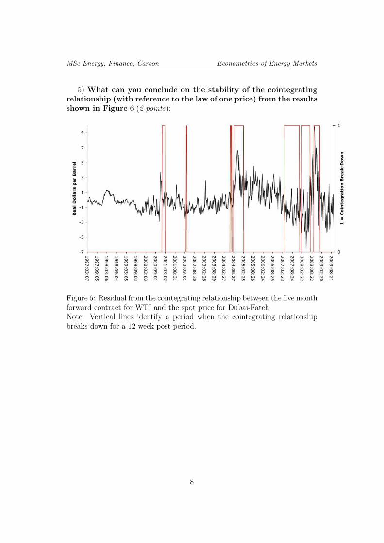
5) What can you conclude on the stability of the cointegratingrelationship (with reference to the law of one price) from the resultsshown in Figure 6 (2 points):

Figure 6: Residual from the cointegrating relationship between the five monthforward contract for WTI and the spot price for Dubai-FatehNote: Vertical lines identify a period when the cointegrating relationshipbreaks down for a 12-week post period.

8


If speculative expectations play an important role in price formation, thecointegrating relationship dictated by the law of one price could break downfor extended periods.

To test for a break down in the long-run cointegrating relationship be-tween the five month contract for WTI and the spot price for Dubai-Fateh,the author uses a test statistic developed by Andrews and Kim (2006):

R =T+m∑

t=T+1

(

T+m∑

s=t

µt

)2

(3)

where (µ) is the residual from the cointegrating relationship for the priceof the two crude oils, m is the length of the post break sample period (12weeks), and T is the end of the pre-break period during which the prices forthe two crude oils cointegrate. The test statistic evaluates the null hypothesisthat the cointegrating relationship does not change in the post break downperiod relative to the pre break period.

6) What can you conclude on the break down in the cointegrat-ing relationship (with reference to Andrews and Kim’s (2006) teststatistic) from the results shown in Figure 6? (2 points)

9

Exercice 3 ( 10 points)

This exercise is based on the paper « Co-integration of ICE Gas Oil and Crude oil futures », Westgaard

et al., Energy Economics, 2011, 311-320.

In this paper, the authors study the spread between ICE1 Gas oil and Crude oil futures prices with

various length up to 12 months. This is also defined as the “crack spread”, as gas oil is produced

when oil is “cracked” in refineries.

The authors expect Gas oil and Brent Crude oil futures traded on ICE Futures Europe to be co-

integrated. In this case, the spread between them will be stationary.

The authors use daily futures prices. The different contracts’ lengths are 1, 2 , 3 , 6 and 12 months.

The crude oil prices series are named C and the Gas oil contracts G with numbers indicating the

length of the contract: C1, C2,…C12, G1,..,G12. The natural logarithm of prices are defined as lnC and

lnG. The natural logarithm of price differences from day t-1 to day t are defined as lnDC and lnDG

respectively. The price differences between contracts is defined as GC = G-C for a given maturity

(GC1, GC2,…GC12).

Data include 3958 observations from 15 april 1994 to 9 november 2009 for the 1 and 2 months

contracts. For the 3,6 and 12 months contracts, daily prices are collected from 1 march 2002 to 9

november 2009 and include 3956 observations.

1. In figure 3 above are displayed the prices for the different maturities. What conclusion can

you make about the behavior of each single serie and the hypothesis of co-integration

between Gas Oil price G and Crude oil price C?

1 ICE : Intercontinental Exchange London.

2. The authors give the following statistics for each prices in natural logarithm.

Augmented Dickey Fuller test are run with a constant, a trend and two lagged difference

variables.

a. Do the prices follow a normal (gaussian distribution) and why?

b. Are the prices autocorrelated and why?

c. Do the prices have a unit root and why?

3. On the following table, you find the same information for the difference of the natural

logarithm of prices

a. Do the price log-difference follow a normal

(gaussian distribution) and why?

b. Are the price log-difference autocorrelated and why?

c. Do the price log-difference have a unit root and why? What conclusion can you infer

about the behavior of the prices in log?

d. Are the required conditions for a test for co-integration between each lnCi and lnGi

satisfied?

4. In a first step, the authors focus of the behavior of the crack spreadt = price Gas oil,t – price Crude

oil, t for each contract length.

a. Suppose the crack spread is stationary. Can we conclude that price Gas oil,t and price Crude oil,t

are cointegrated? What is the cointegrating relationship in this case?

b. The following figures display the crack spread for each contract length. For which

contract length we have more chance to find a cointegration relations between price Gas

oil,t and price Crude oil,t ?

c. The following table gives you some statistics for the different crack spread. For which

contract length, answer if the spread is stationary or not. For which length do we find

cointegration between price Gas oil,t and price Crude oil,t ?

5. The authors now apply the Johansen test for co-integration. For each contract length, they

report the result of the test of 0 against 1 co-integration relation. The results are the

following

a. For each case, say if we accept or reject the hypothesis of 0 cointegration relation. You

can consider different critical level for the test.

b. According to the previous results, what can you conclude about the robustness of results

to the contract length?

c. What can you say about the robustness of results to the time period? What difference

characterizes these two time periods and could explain these results?

Econometrie des marches de l’energie

Examen Partiel

Yannick Le Pen, Julien Chevallier

Jeudi 22 mars 2012

Exercice I (10 points)

Cet exercice utilise les resultats publies dans l’article de Brown et Yucel (2008) ”What drives natural gasprices?”, The Energy journal, 29(2), 45-60.

Les auteurs de cet article etudient la relation entre le prix du gaz naturel et le prix du petrole brut aux Etats-Unis. L’objectif est de verifier si le prix du gaz naturel suit l’evolution du prix du petrole brut, ce dernier etantfixe sur le marche mondial. La principale raison d’une relation entre ces deux prix est la possibilite techniquede passer assez rapidement de l’une a l’autre de ces deux sources d’energie, notamment dans la productiond’electricite. Cet effet de substitution empecherait les prix de s’eloigner l’un de l’autre a long terme.

Les auteurs utilisent des series hebdomadaires sur la periode du 13 juin 1997 au 8 juin 2007. Ils considerentles variables suivantes :

• PHH prix du gas naturel Henry Hub 1

• PWTI prix du petrole brut West Texas Intermediate (WTI)2

Les auteurs veulent de plus evaluer l’effet d’autres variables sur la relation entre les prix du gaz naturel et dupetrole. Ils considerent les variables suivantes :

• HDD : heating degree days

• HDDDEV : deviations above normal heating degree days

• CDD : cooling degree days

• CDD : deviations above cooling degree days

• Storage diff : difference entre les stocks a une semaine t et la moyenne des stocks pour cette meme semaineau cours des 5 annees precedentes

• SHUT IN : evenement ponctuel (du type ouragan) interrompant la production.

Dans un premier temps, les auteurs verifient si les series utilisees sont stationnaires ou non. Il utilisent le testde Dickey-Fuller augmente et resument leurs resultats dans le tableau 1 Unit Root Tests.

1Henry Hub, pres de la Nouvelle Orleans est le noeud par lequel transite le plus grand volume de gaz naturel aux Etats-Unis.Il est proche des regions ou se concentrent les plus grands gisements de gaz naturel conventionnels.

2Le West Texas Intermediate est un type de petrole souvent utilise comme benchmark pour la fixation du prix du brut, commepar exemple le Brent (mer du nord) en Europe.

1

1. Decrivez le test de racine unitaire de Dickey-Fuller augmente: hypotheses nulle et alternative, equationestimee, statistique de test.

2. Indiquez, en justifiant vos reponses, quelles variables peuvent etre interpretees comme stationnaires etnon stationnaires a l’issue de ce test ? Pour quelle raison, la colonne ”First difference” ne contient pas unresultat pour toutes les series ?

3. En vous appuyant sur la definition de la stationnarite du second ordre, pouvait-on anticiper intuitivementde tels resultats ?

Les auteurs verifient maintenant l’existence d’une relation de cointegration entre le prix du gas naturel et leprix du petrole. Ils considerent la relation de cointegration suivante :

ln(PHH,t) = γ + βln(PWTI,t) + ut

4. Les conditions d’application d’un test de cointegration sont-elles satisfaites ? Combien de relations decointegration peut-on theoriquement obtenir entre ces deux variables.

5. Les resultats du test de cointegration de Johansen sont reportes dans le tableau 2 Bi-Variate Cointe-gration Tests. Existe-t-il des relations de cointegration ? si oui, ecrire cette relation.

6. Que peut-on dire que l’effet a long terme d’une augmentation de 1% du prix du petrole sur celui du gaznaturel ?

Les auteurs integrent la relation de cointegration representee par CIt−1 dans le modele a correction d’erreur(MCE) suivant :

∆PHH,t = a+ αCIt−1 +

n∑i=1

bi∆PWTI,t−i +

n∑i=1

ci∆PHH,t−i + εt

7. Donnez l’expression de CIt−1.

8. Decrivez comment la variation du prix du gas naturel est decomposee dans le modele a correction d’erreur?

9. L’estimation du MCE est donnee dans le tableau 3 Error-Correction Models of the Change inNatural Gas Price. La relation de cointegration intervient-elle vraiment dans la dynamique du prix dugaz naturel ? Quel sera l’effet d’un prix du gaz surevalue par rapport a sa valeur de long terme sur lavariation a court terme ? Est-ce conforme a l’effet attendu ?

Les auteurs ajoutent les variables de temperature, de stock et d’evenements climatiques au MCE :

∆PHH,t = a +αCIt−1 +

n∑i=1

bi∆PWTI,t−i +

n∑i=1

ci∆PHH,t−i + d1HDDt + d2HDDDEVt

+ d3CDDt + d4CDDDEVt + d5STORDIFFt + d6SHUTINt + εt

10. Compte tenue de leur caracterisation, peut-on ajouter ces variables sans risque de regression mal specifiee(spurious regression)?

11. Ces variables supplementaires sont-elles significatives et augmentent-elles le pouvoir explicatif du MCE ?

12. Le prix du petrole cause-t-il le prix du gaz naturel ?

2

Exercice II (10 points)

Cet exercice est base sur l’article de Ying Fan et Jin-Hua Xu intitule ‘What has driven oil prices since 2000? Astructural change perspective’ et publie dans la revue Energy Economics 33 (2011), 1082-1094.

La periode couverte dans cet article est: 7 Janvier 2000 - 11 Septembre 2009.

Considerez le modele de fondamentaux du prix du petrole suivant:

pt = αi + βoi(L)pt + βgi(L)goldt + βsi(L)bdit + βui(L)usdxt + βpi(L)sp500t + εt (1)

avec pt la transformation logarithmique du prix futures du petrole West Texas Intermediate (WTI), goldt latransformation logarithmique du prix futures de l’or Commodity Exchange (COMEX), bdit la transformationlogarithmique du Baltic Dry Index3, usdxt la transformation logarithmique de l’US Dollar Index4, sp500t latransformation logarithmique de l’index US S&P 5005, εt le terme d’erreur, L l’operateur retard et LXt = Xt−1.Les coefficients βoi(L), βgi(L), βsi(L), βui(L), βpi(L) sont des polynomes en L.

Question #13 (0,5 point)

Rappelez brievement l’interet de la transformation logarithmique des variables dans le modele represente parl’equation (1).

Question #14 (1 point)

Quelle(s) remarque(s) pouvez-vous enoncez avant meme l’analyse econometrique concernant la validite et lapertinence de ce modele (Eq.(1))?

Considerez a present un modele alternatif de fondamentaux du prix du petrole:

pt =αi + βoi(L)pt + βgi(L)goldt + βsi(L)bdit + βui(L)usdxt + βpi(L)sp500t

+ βn1i(L)noncomm1t + +βn2i(L)noncomm2t + φiD01t + λiD03t + εt(2)

avec noncomm1t la difference premiere de la position (en %) des agents non-commerciaux6, noncomm2tla difference premiere de la position longue (en %) des agents non-commerciaux, D01t une variable indica-trice (dummy) capturant les attaques terroristes du 11 Septembre, et D03t une variable indicatrice (dummy)capturant les effets de la Seconde Guerre du Golfe.

3Le Baltic Dry Index est une mesure des fondamentaux offre-demande sur le marche du petrole. Il s’agit d’un indicateur decroissance economique base sur le taux de remplissage des cargos.

4L’US Dollar Index represente la valeur du dollar en comparaison avec un panier d’autres monnaies etrangeres.5L’index Standard & Poor’s 500 est une mesure mondiale des marches d’action.6La Commodities Futures Trading Commission (CFTC) distingue 2 types d’agents intervenant sur le marche du petrole: les

agents commerciaux (producteurs et exportateurs de petrole) interesses par la delivrance physique du barril de petrole, et les agentsnon-commerciaux (banques d’investissement, hedge fund, traders, brokers) interesses par le trading de produits derives sans notionde delivrance physique du produit.

5

Question #15 (1,5 points)

Quelles sont les principales differences entre les modeles de fondamentaux du prix du petrole decrit par lesequations (1) et (2)?

En quoi l’Eq.(2) repond-t-elle a des limitations que vous aviez pu identifier dans votre reponse a la questionprecedente?

6

Question #16 (3 points)

Considerez les resultats d’estimation reproduits dans le Tableau 6 ‘Full period results’ sur la periode completeallant du 7 Janvier 2000 au 11 Septembre 2009:

• Commentez la significativite statistique de chaque variable pour les 2 premieres colonnes.

• Deduisez-en des interpretations economiques en terme de fondamentaux du prix du petrole.

• Quel est l’interet d’avoir estime une nouvelle fois le modele dans la 3eme colonne?


A la lecture du Tableau 7 ‘Relatively calm market period results’, vos conclusions demurent-elles inchangeessur la sous-periode allant du 7 Janvier 2000 au 12 Mars 2004?

7


Le Tableau 8 ‘Bubble accumulation period and Global economic crisis period results’ couvre 2 autres sous-periodes:

1. du 19 Mars 2004 au 06 Juin 2008: quelles sont les raisons pouvant justifier la formation d’une bullespeculative sur le marche du petrole? quelles sont vos conclusions d’apres les resultats d’estimation?

2. du 13 Juin 2008 au 11 Septembre 2009: la crise financiere a-t-elle conduit a un changement de fondamen-taux sur le marche du petrole? Justifiez votre reponse en fonction des resultats d’estimation.

8

Econometrics of Energy Markets - Centre de Recherche …€¦ · Students will be trained with the...

Documents

Transcript of Econometrics of Energy Markets - Centre de Recherche …€¦ · Students will be trained with the...