Econometrics and Quantitative Chapter 1site.iugaza.edu.ps/ssafi/files/2012/09/Lectures-20121.pdf ·...

1-٠© 2011 Pearson Addison-Wesley. All rights reserved.

Econometrics and Quantitative Analysis

Using Econometrics: A Practical Guide

A.H. Studenmund

6th Edition. Addison Wesley Longman

Instructor: Dr. Samir Safi

Associate Professor of Statistics

Fall 2012

Chapter 1

An Overview of Regression

Analysis

Copyright © 2011 Pearson Addison-Wesley.

All rights reserved.

Slides by Niels-Hugo BlunchWashington and Lee University

1-٢© 2011 Pearson Addison-Wesley. All rights reserved.

What is Econometrics?

• Econometrics literally means “economic measurement”

• It is the quantitative measurement and analysisof actual economic and business phenomena—and so involves:

– economic theory

– Statistics

– Math

– observation/data collection

1-٣© 2011 Pearson Addison-Wesley. All rights reserved.

What is Econometrics? (cont.)

• Three major uses of econometrics:

– Describing economic reality

– Testing hypotheses about economic theory

– Forecasting future economic activity

• So econometrics is all about questions: the researcher (YOU!) first asks questions and then uses econometrics to answer them

1-٤© 2011 Pearson Addison-Wesley. All rights reserved.

Example

• Consider the general and purely theoretical relationship:

Q = f(P, Ps, Yd) (1.1)

• Econometrics allows this general and purely theoretical relationship to become explicit:

Q = 27.7 – 0.11P + 0.03Ps + 0.23Yd (1.2)

1-٥© 2011 Pearson Addison-Wesley. All rights reserved.

What is Regression Analysis?

• Economic theory can give us the direction of a change, e.g. the change in the demand for dvd’s following a price decrease (or price increase)

• But what if we want to know not just “how?” but also “how much?”

• Then we need:

– A sample of data

– A way to estimate such a relationship

• one of the most frequently ones used is regression analysis

1-٦© 2011 Pearson Addison-Wesley. All rights reserved.

What is Regression Analysis? (cont.)

• Formally, regression analysis is a statistical technique that attempts to “explain”movements in one variable, the dependentvariable, as a function of movements in a set of other variables, the independent (or explanatory) variables, through the quantification of a single equation

1-٧© 2011 Pearson Addison-Wesley. All rights reserved.

Example

• Return to the example from before:

Q = f(P, Ps, Yd) (1.1)

• Here, Q is the dependent variable and P, Ps, Yd are the independent variables

• Don’t be deceived by the words dependent and independent, however

– A statistically significant regression result does not necessarily imply causality

– We also need:

• Economic theory

• Common sense

1-٨© 2011 Pearson Addison-Wesley. All rights reserved.

Single-Equation Linear Models

• The simplest example is:

Y = + X (1.3)

• The are denoted “coefficients”

– is the “constant” or “intercept” term

– is the “slope coefficient”: the amount that Y will change when X increases by one unit; for a linear model, is constant over the entire function

0β1

β

' sβ

0β

1β

1β

1-٩© 2011 Pearson Addison-Wesley. All rights reserved.

Figure 1.1Graphical Representation of the

Coefficients of the Regression Line

1-١٠© 2011 Pearson Addison-Wesley. All rights reserved.

Single-Equation Linear Models (cont.)

• Application of linear regression techniques requires that the equation be linear—such as (1.3)

• By contrast, the equation

Y = + X2 (1.4)

is not linear

• What to do? First define

Z = X2 (1.5)

• Substituting into (1.4) yields:

Y = + Z (1.6)

• This redefined equation is now linear (in the coefficients and in the variables Y and Z)

0β

0β

0β

1β

1β

1β

1-١١© 2011 Pearson Addison-Wesley. All rights reserved.


• Is (1.3) a complete description of origins of variation in Y?

• No, at least four sources of variation in Y other than the variation in the included Xs:

• Other potentially important explanatory variables may be missing(e.g., X2 and X3)

• Measurement error

• Incorrect functional form

• Purely random and totally unpredictable occurrences

• Inclusion of a “stochastic error term” (ε) effectively “takes care” of all these other sources of variation in Y that are NOT captured by X, so that (1.3) becomes:

Y = β0 + β1X + ε (1.7)

1-١٢© 2011 Pearson Addison-Wesley. All rights reserved.


• Two components in (1.7):

– deterministic component (β0 + β1X)

– stochastic/random component (ε)

• Why “deterministic”?

– Indicates the value of Y that is determined by a given value of X (which is assumed to be non-stochastic)

– Alternatively, the det. comp. can be thought of as the expected value of Y given X—namely E(Y|X)—i.e. the mean (or average) value of the Ys associated with a particular value of X

– This is also denoted the conditional expectation (that is, expectation of Y conditional on X)

1-١٣© 2011 Pearson Addison-Wesley. All rights reserved.

Example: Aggregate Consumption Function

• Aggregate consumption as a function of aggregate income may be lower (or higher) than it would otherwise have been due to:– consumer uncertainty—hard (impossible?) to measure, i.e. is an

omitted variable

– Observed consumption may be different from actual consumption due to measurement error

– The “true” consumption function may be nonlinear but a linear one is estimated (see Figure 1.2 for a graphical illustration)

– Human behavior always contains some element(s) of pure chance; unpredictable, i.e. random events may increase or decrease consumption at any given time

• Whenever one or more of these factors are at play, the observed Y will differ from the Y predicted from the deterministic part, β0 + β1X

1-١٤© 2011 Pearson Addison-Wesley. All rights reserved.

Figure 1.2 Errors Caused by Using a Linear Functional

Form to Model a Nonlinear Relationship

1-١٥© 2011 Pearson Addison-Wesley. All rights reserved.

Extending the Notation

• Include reference to the number of observations

– Single-equation linear case:

Yi = β0 + β1Xi + εi (i = 1,2,…,N) (1.10)

• So there are really N equations, one for each observation

• the coefficients, β0 and β1, are the same

• the values of Y, X, and ε differ across observations

1-١٦© 2011 Pearson Addison-Wesley. All rights reserved.

Extending the Notation (cont.)

• The general case: multivariate regression

Yi = β0 + β1X1i + β2X2i + β3X3i + εi (i = 1,2,…,N)(1.11)

• Each of the slope coefficients gives the impact of a one-unit increase in the corresponding X variable on Y, holding the other included independent variables constant (i.e., ceteris paribus)

• As an (implicit) consequence of this, the impact of variables that are not included in the regression are not held constant (we return to this in Ch. 6)

1-١٧© 2011 Pearson Addison-Wesley. All rights reserved.

Example: Wage Regression

• Let wages (WAGE) depend on:

– years of work experience (EXP)

– years of education (EDU)

– gender of the worker (GEND: 1 if male, 0 if female)

• Substituting into equation (1.11) yields:

WAGEi = β0 + β1EXPi + β2EDUi + β3GENDi + εi

(1.12)

1-١٨© 2011 Pearson Addison-Wesley. All rights reserved.

Indexing Conventions

• Subscript “i” for data on individuals (so called “cross section” data)

• Subscript “t” for time series data (e.g., series of years, months, or days—daily exchange rates, for example )

• Subscript “it” when we have both (for example, “panel data”)

1-١٩© 2011 Pearson Addison-Wesley. All rights reserved.

The Estimated Regression Equation

• The regression equation considered so far is the “true”—but unknown—theoretical regression equation

• Instead of “true,” might think about this as the populationregression vs. the sample/estimated regression

• How do we obtain the empirical counterpart of the theoretical regression model (1.14)?

• It has to be estimated

• The empirical counterpart to (1.14) is:

(1.16)

• The signs on top of the estimates are denoted “hat,” so that we have “Y-hat,” for example

iiXY 10

ˆˆˆ ββ +=

1-٢٠© 2011 Pearson Addison-Wesley. All rights reserved.

The Estimated Regression Equation (cont.)

• For each sample we get a different set of estimated regression coefficients

• Y is the estimated value of Yi (i.e. the dependent variable for observation i); similarly it is the prediction of E(Yi|Xi) from the regression equation

• The closer Y is to the observed value of Yi, the better is the “fit” of the equation

• Similarly, the smaller is the estimated error term, ei, often denoted the “residual,” the better is the fit

1-٢١© 2011 Pearson Addison-Wesley. All rights reserved.

The Estimated Regression Equation (cont.)

• This can also be seen from the fact that

(1.17)

• Note difference with the error term, εi, given as

(1.18)

• This all comes together in Figure 1.3

1-٢٢© 2011 Pearson Addison-Wesley. All rights reserved.

Figure 1.3 True and Estimated Regression Lines

1-٢٣© 2011 Pearson Addison-Wesley. All rights reserved.

Example: Using Regression to Explain Housing prices

• Houses are not homogenous products, like corn or gold, that have generally known market prices

• So, how to appraise a house against a given asking price?

• Yes, it’s true: many real estate appraisers actually use regression analysis for this!

• Consider specific case: Suppose the asking price was $230,000

1-٢٤© 2011 Pearson Addison-Wesley. All rights reserved.

Example: Using Regression to Explain Housing prices (cont.)

• Is this fair / too much /too little?

• Depends on size of house (higher size, higher price)

• So, collect cross-sectional data on prices (in thousands of $) and sizes (in square feet) for, say, 43 houses

• Then say this yields the following estimated regression line:

(1.23)ii

SIZECEIPR 138.00.40ˆ +=

1-٢٥© 2011 Pearson Addison-Wesley. All rights reserved.

Figure 1.5 A Cross-Sectional Model of Housing Prices

1-٢٦© 2011 Pearson Addison-Wesley. All rights reserved.


• Note that the interpretation of the intercept term is problematic in this case (we’ll get back to this later, in Section 7.1.2)

• The literal interpretation of the intercept here is the price of a house with a size of zero square feet…

1-٢٧© 2011 Pearson Addison-Wesley. All rights reserved.


• How to use the estimated regression line / estimated regression coefficients to answer the question?

– Just plug the particular size of the house, you are interested in (here, 1,600 square feet) into (1.23)

– Alternatively, read off the estimated price using Figure 1.5

• Either way, we get an estimated price of $260.8 (thousand, remember!)

• So, in terms of our original question, it’s a good deal—go ahead and purchase!!

• Note that we simplified a lot in this example by assuming that only size matters for housing prices

1-٢٨© 2011 Pearson Addison-Wesley. All rights reserved.

Table 1.1a Data for and Results of the Weight-Guessing Equation

1-٢٩© 2011 Pearson Addison-Wesley. All rights reserved.

Table 1.1b Data for and Results of the Weight-Guessing Equation

1-٣٠© 2011 Pearson Addison-Wesley. All rights reserved.

Figure 1.4 A Weight-Guessing Equation

1-٣١© 2011 Pearson Addison-Wesley. All rights reserved.

Key Terms from Chapter 1

• Regression analysis

• Dependent variable

• Independent (or explanatory) variable(s)

• Causality

• Stochastic error term

• Linear

• Intercept term

• Slope coefficient

• Multivariate regression model

• Expected value

• Residual

• Time series

• Cross-sectional data set

1-٣٢© 2011 Pearson Addison-Wesley. All rights reserved.

Chapter 2

Ordinary Least Squares

1-٣٣© 2011 Pearson Addison-Wesley. All rights reserved. 2-٣٣© 2011 Pearson Addison-Wesley. All rights reserved.

Estimating Single-Independent-Variable Models with OLS

• Recall that the objective of regression analysis is to start from:

(2.1)

• And, through the use of data, to get to:

(2.2)

• Recall that equation 2.1 is purely theoretical, while equation (2.2) is it empirical counterpart

• How to move from (2.1) to (2.2)?

1-٣٤© 2011 Pearson Addison-Wesley. All rights reserved. 2-٣٤© 2011 Pearson Addison-Wesley. All rights reserved.

Estimating Single-Independent-Variable Models with OLS (cont.)

• One of the most widely used methods is Ordinary Least Squares (OLS)

• OLS minimizes (i = 1, 2, …., N) (2.3)

• Or, the sum of squared deviations of the vertical distancebetween the residuals (i.e. the estimated error terms) and the estimated regression line

• We also denote this term the “Residual Sum of Squares”(RSS)

1-٣٥© 2011 Pearson Addison-Wesley. All rights reserved. 2-٣٥© 2011 Pearson Addison-Wesley. All rights reserved.


• Similarly, OLS minimizes:

• Why use OLS?

• Relatively easy to use

• The goal of minimizing RSS is intuitively / theoretically appealing

• This basically says we want the estimated regression equation to be as close as possible to the observed data

• OLS estimates have a number of useful characteristics

2)ˆ(

i

N

i

iYY −∑

1-٣٦© 2011 Pearson Addison-Wesley. All rights reserved. 2-٣٦© 2011 Pearson Addison-Wesley. All rights reserved.


• OLS estimates have at least two useful characteristics:

• The sum of the residuals is exactly zero

• OLS can be shown to be the “best” estimator when certain specific conditions hold (we’ll get back to this in Chapter 4)

– Ordinary Least Squares (OLS) is an estimator

– A given produced by OLS is an estimate

1-٣٧© 2011 Pearson Addison-Wesley. All rights reserved. 2-٣٧© 2011 Pearson Addison-Wesley. All rights reserved.


How does OLS work?

• First recall from (2.3) that OLS minimizes the sum of the squared residuals

• Next, it can be shown (see Exercise 12) that the coefficients that ensure that for the case of just one independent variable are:

(2.4)

(2.5)

1-٣٨© 2011 Pearson Addison-Wesley. All rights reserved. 2-٣٨© 2011 Pearson Addison-Wesley. All rights reserved.

Estimating Multivariate Regression Models with OLS

• In the “real world” one explanatory variable is not enough

• The general multivariate regression model with K independent variables is:

Yi = β0 + β1X1i + β2X2i + ... + βKXKi + εi (i = 1,2,…,N)(1.13)

• Biggest difference with single-explanatory variable regression model is in the interpretation of the slope coefficients

– Now a slope coefficient indicates the change in the dependent variable associated with a one-unit increase in the explanatory variable holding the other explanatory variables constant

1-٣٩© 2011 Pearson Addison-Wesley. All rights reserved. 2-٣٩© 2011 Pearson Addison-Wesley. All rights reserved.

Estimating Multivariate Regression Models with OLS (cont.)

• Omitted (and relevant!) variables are therefore not

held constant

• The intercept term, β0, is the value of Y when all the Xs and the error term equal zero

• Nevertheless, the underlying principle of minimizing the summed squared residuals remains the same

1-٤٠© 2011 Pearson Addison-Wesley. All rights reserved. 2-٤٠© 2011 Pearson Addison-Wesley. All rights reserved.

Example: financial aid awards at a liberal arts college

• Dependent variable:

• FINAIDi: financial aid (measured in dollars of grant) awarded to the ith applicant

1-٤١© 2011 Pearson Addison-Wesley. All rights reserved. 2-٤١© 2011 Pearson Addison-Wesley. All rights reserved.

Example: financial aid awards at a liberal arts college

• Theoretical Model:

(2.9)

(2.10)

where:

– PARENTi: The amount (in dollars) that the parents of the ith student are judged able to contribute to college expenses

– HSRANKi: The ith student’s GPA rank in high school, measured as a percentage (i.e. between 0 and 100)

1-٤٢© 2011 Pearson Addison-Wesley. All rights reserved. 2-٤٢© 2011 Pearson Addison-Wesley. All rights reserved.

Example: financial aid awards at a liberal arts college (cont.)

• Estimate model using the data in Table 2.2 to get:

(2.11)

• Interpretation of the slope coefficients?

– Graphical interpretation in Figures 2.1 and 2.2

1-٤٣© 2011 Pearson Addison-Wesley. All rights reserved. 2-٤٣© 2011 Pearson Addison-Wesley. All rights reserved.

Figure 2.1 Financial Aid as a Function of Parents’ Ability to Pay

1-٤٤© 2011 Pearson Addison-Wesley. All rights reserved. 2-٤٤© 2011 Pearson Addison-Wesley. All rights reserved.

Figure 2.2 Financial Aid as a Function of High School Rank

1-٤٥© 2011 Pearson Addison-Wesley. All rights reserved. 2-٤٥© 2011 Pearson Addison-Wesley. All rights reserved.

Total, Explained, and Residual Sums of Squares

• (2.12)

• (2.13)

• TSS = ESS + RSS

• This is usually called the decomposition of variance

1-٤٦© 2011 Pearson Addison-Wesley. All rights reserved. 2-٤٦© 2011 Pearson Addison-Wesley. All rights reserved.

Figure 2.3 Decomposition of the

Variance in Y

1-٤٧© 2011 Pearson Addison-Wesley. All rights reserved. 2-٤٧© 2011 Pearson Addison-Wesley. All rights reserved.

Evaluating the Quality of a Regression Equation

Checkpoints here include the following:

1. Is the equation supported by sound theory?

2. How well does the estimated regression fit the data?

3. Is the data set reasonably large and accurate?

4. Is OLS the best estimator to be used for this equation?

5. How well do the estimated coefficients correspond to the expectationsdeveloped by the researcher before the data were collected?

6. Are all the obviously important variables included in the equation?

7. Has the most theoretically logical functional form been used?

8. Does the regression appear to be free of major econometric problems?

*These numbers roughly correspond to the relevant chapters in the book

1-٤٨© 2011 Pearson Addison-Wesley. All rights reserved. 2-٤٨© 2011 Pearson Addison-Wesley. All rights reserved.

Describing the Overall Fit of the Estimated Model

• The simplest commonly used measure of overall fit is the coefficient of determination, R2:

(2.14)

• Since OLS selects the coefficient estimates that minimizes RSS, OLS provides the largest possible R2 (within the class of linear models)

1-٤٩© 2011 Pearson Addison-Wesley. All rights reserved. 2-٤٩© 2011 Pearson Addison-Wesley. All rights reserved.

Figure 2.4 Illustration of Case Where R2 = 0

1-٥٠© 2011 Pearson Addison-Wesley. All rights reserved. 2-٥٠© 2011 Pearson Addison-Wesley. All rights reserved.

Figure 2.5 Illustration of Case Where R2 = .95

1-٥١© 2011 Pearson Addison-Wesley. All rights reserved. 2-٥١© 2011 Pearson Addison-Wesley. All rights reserved.

Figure 2.6 Illustration of Case Where R2 = 1

1-٥٢© 2011 Pearson Addison-Wesley. All rights reserved. 2-٥٢© 2011 Pearson Addison-Wesley. All rights reserved.

The Simple Correlation Coefficient, r

• This is a measure related to R2

• r measures the strength and direction of the linear relationship between two variables:

– r = +1: the two variables are perfectly positivelycorrelated

– r = –1: the two variables are perfectly negativelycorrelated

– r = 0: the two variables are totally uncorrelated

1-٥٣© 2011 Pearson Addison-Wesley. All rights reserved. 2-٥٣© 2011 Pearson Addison-Wesley. All rights reserved.

The adjusted coefficient of determination

• A major problem with R2 is that it can never decrease if another independent variable is added

• An alternative to R2 that addresses this issue is the adjusted R2 or R2:

(2.15)

Where N – K – 1 = degrees of freedom

1-٥٤© 2011 Pearson Addison-Wesley. All rights reserved. 2-٥٤© 2011 Pearson Addison-Wesley. All rights reserved.

The adjusted coefficient of determination (cont.)

• So, R2 measures the share of the variation of Y around its mean that is explained by the regression equation, adjusted for degrees of freedom

• R2 can be used to compare the fits of regressions with the same dependent variable and different numbers of independent variables

• As a result, most researchers automatically use instead of R2 when evaluating the fit of their estimated regressions equations

1-٥٥© 2011 Pearson Addison-Wesley. All rights reserved. 2-٥٥© 2011 Pearson Addison-Wesley. All rights reserved.

Table 2.1a The Calculation of Estimated Regression

Coefficients for the Weight/Height Example

1-٥٦© 2011 Pearson Addison-Wesley. All rights reserved. 2-٥٦© 2011 Pearson Addison-Wesley. All rights reserved.

Table 2.1b The Calculation of Estimated Regression

Coefficients for the Weight/Height Example

1-٥٧© 2011 Pearson Addison-Wesley. All rights reserved. 2-٥٧© 2011 Pearson Addison-Wesley. All rights reserved.

Table 2.2a Data for the Financial Aid Example

1-٥٨© 2011 Pearson Addison-Wesley. All rights reserved. 2-٥٨© 2011 Pearson Addison-Wesley. All rights reserved.

Table 2.2b Data for the Financial Aid Example

1-٥٩© 2011 Pearson Addison-Wesley. All rights reserved. 2-٥٩© 2011 Pearson Addison-Wesley. All rights reserved.

Table 2.2c Data for the Financial Aid Example

1-٦٠© 2011 Pearson Addison-Wesley. All rights reserved. 2-٦٠© 2011 Pearson Addison-Wesley. All rights reserved.

Table 2.2d Data for the Financial Aid Example

1-٦١© 2011 Pearson Addison-Wesley. All rights reserved. 2-٦١© 2011 Pearson Addison-Wesley. All rights reserved.


• Ordinary Least Squares (OLS)

• Interpretation of a multivariate regression coefficient

• Total sums of squares

• Explained sums of squares

• Residual sums of squares

• Coefficient of determination, R2

• Simple correlation coefficient, r

• Degrees of freedom

• Adjusted coefficient of determination , R2

1-٦٢© 2011 Pearson Addison-Wesley. All rights reserved.

Chapter 3

Learning to Use Regression Analysis

1-٦٣© 2011 Pearson Addison-Wesley. All rights reserved.

Steps in Applied Regression Analysis

• The first step is choosing the dependent variable – this step is determined by the purpose of the research (see Chapter 11 for details)

• After choosing the dependent variable, it’s logical to follow the following sequence:

1. Review the literature and develop the theoretical model

2. Specify the model: Select the independent variables and the functional form

3. Hypothesize the expected signs of the coefficients

4. Collect the data. Inspect and clean the data

5. Estimate and evaluate the equation

6. Document the results

1-٦٤© 2011 Pearson Addison-Wesley. All rights reserved.

Step 1: Review the Literature and Develop the Theoretical Model

• Perhaps counter intuitively, a strong theoretical foundation is the best start for any empirical project

• Reason: main econometric decisions are determined by the underlying theoretical model

• Useful starting points:

– Journal of Economic Literature or a business oriented publication of abstracts

– Internet search, including Google Scholar

– EconLit, an electronic bibliography of economics literature (for more details, go to www.EconLit.org)

1-٦٥© 2011 Pearson Addison-Wesley. All rights reserved.

Step 2: Specify the Model: Independent Variables and Functional Form

• After selecting the dependent variable, the specification of a model involves choosing the following components:

1. the independent variables and how they should be measured,

2. the functional (mathematical) form of the variables, and

3. the properties of the stochastic error term

1-٦٦© 2011 Pearson Addison-Wesley. All rights reserved.

Step 2: Specify the Model: Independent Variables and

Functional Form (cont.)

• A mistake in any of the three elements results in a specification error

• For example, only theoretically relevant explanatory variables should be included

• Even so, researchers frequently have to make choices –also denoted imposing their priors

• Example:

• when estimating a demand equation, theory informs us that prices of complements and substitutes of the good in question are important explanatory variables

• But which complements—and which substitutes?

1-٦٧© 2011 Pearson Addison-Wesley. All rights reserved.

Step 3: Hypothesize the Expected Signs of the Coefficients

• Once the variables are selected, it’s important to hypothesize the expected signs of the regression coefficients

• Example: demand equation for a final consumption good

• First, state the demand equation as a general function:

(3.2)

• The signs above the variables indicate the hypothesized sign of the respective regression coefficient in a linear model

1-٦٨© 2011 Pearson Addison-Wesley. All rights reserved.

Step 4: Collect the Data & Inspect and Clean the Data

• A general rule regarding sample size is “the more observations the better”

• as long as the observations are from the same general population!

• The reason for this goes back to notion of degrees of freedom (mentioned first in Section 2.4)

• When there are more degrees of freedom:

• Every positive error is likely to be balanced by a negative error (see Figure 3.2)

• The estimated regression coefficients are estimated with a greater deal of precision

1-٦٩© 2011 Pearson Addison-Wesley. All rights reserved.

Figure 3.1 Mathematical Fit of a Line to Two Points

1-٧٠© 2011 Pearson Addison-Wesley. All rights reserved.

Figure 3.2 Statistical Fit of a Line to Three Points

1-٧١© 2011 Pearson Addison-Wesley. All rights reserved.

Step 4: Collect the Data & Inspect and Clean the Data (cont.)

• Estimate model using the data in Table 2.2 to get:

• Inspecting the data—obtain a printout or plot (graph) of the data

• Reason: to look for outliers

– An outlier is an observation that lies outside the range of the rest of the observations

• Examples:

– Does a student have a 7.0 GPA on a 4.0 scale?

– Is consumption negative?

1-٧٢© 2011 Pearson Addison-Wesley. All rights reserved.

Step 5: Estimate and Evaluate the Equation

• Once steps 1–4 have been completed, the estimation part is quick

– using Eviews or Stata to estimate an OLS regression takes less than a second!

• The evaluation part is more tricky, however, involving answering the following questions:

– How well did the equation fit the data?

– Were the signs and magnitudes of the estimated coefficients as expected?

• Afterwards may add sensitivity analysis (see Section 6.4 for details)

1-٧٣© 2011 Pearson Addison-Wesley. All rights reserved.

Step 6: Document the Results

• A standard format usually is used to present estimated regression results:

(3.3)

• The number in parentheses under the estimated coefficient is the estimated standard error of the estimated coefficient, and the t-value is the one used to test the hypothesis that the true value of the coefficient is different from zero (more on this later!)

1-٧٤© 2011 Pearson Addison-Wesley. All rights reserved.

Case Study: Using Regression Analysis to Pick Restaurant Locations

• Background:

• You have been hired to determine the best location for the next Woody’s restaurant (a moderately priced, 24-hour, family restaurant chain)

• Objective:

• How to decide location using the six basic steps of applied regression analysis, discussed earlier?

1-٧٥© 2011 Pearson Addison-Wesley. All rights reserved.

Step 1: Review the Literature and Develop the Theoretical Model

• Background reading about the restaurant industry

• Talking to various experts within the firm

– All the chain’s restaurants are identical and located in suburban, retail, or residential environments

– So, lack of variation in potential explanatory variables to helpdetermine location

– Number of customers most important for locational decision

� Dependent variable: number of customers (measured by the number of checks or bills)

1-٧٦© 2011 Pearson Addison-Wesley. All rights reserved.

Step 2: Specify the Model: Independent Variables and Functional Form

• More discussions with in-house experts reveal three major determinants of sales:

– Number of people living near the location

– General income level of the location

– Number of direct competitors near the location

1-٧٧© 2011 Pearson Addison-Wesley. All rights reserved.

Step 2: Specify the Model: Independent Variables and Functional Form (cont.)

• Based on this, the exact definitions of the independent variables you decide to include are:

– N = Competition: the number of direct competitors within a two-mile radius of the Woody’s location

– P = Population: the number of people living within a three-mile radius of the location

– I = Income: the average household income of the population measured in variable P

• With no reason to suspect anything other than linear functional form and a typical stochastic error term, that’s what you decide to use

1-٧٨© 2011 Pearson Addison-Wesley. All rights reserved.

Step 3: Hypothesize the Expected Signs of the Coefficients

• After talking some more with the in-house experts and thinking some more, you come up with the following:

(3.4)

1-٧٩© 2011 Pearson Addison-Wesley. All rights reserved.

Step 4: Collect the Data & Inspect and Clean the Data

• You manage to obtain data on the dependent and independent variables for all 33 Woody’s restaurants

• Next, you inspect the data

• The data quality is judged as excellent because:

• Each manager measures each variable identically

• All restaurants are included in the sample

• All information is from the same year

• The resulting data is as given in Tables 3.1 and 3.3 in the book (using Eviews and Stata, respectively)

1-٨٠© 2011 Pearson Addison-Wesley. All rights reserved.

Step 5: Estimate and Evaluate the Equation

• You take the data set and enter it into the computer

• You then run an OLS regression (after thinking the model over one last time!)

• The resulting model is:

Estimated coefficients are as expected and the fit is reasonable

• Values for N, P, and I for each potential new location are then obtained and plugged into (3.5) to predict Y

(3.5)

1-٨١© 2011 Pearson Addison-Wesley. All rights reserved.

Step 6: Document the Results

• The results summarized in Equation 3.5 meet our documentation requirements

• Hence, you decide that there’s no need to take this step any further

1-٨٢© 2011 Pearson Addison-Wesley. All rights reserved.

Table 3.1aData for the Woody’s Restaurants Example

(Using the Eviews Program)

1-٨٣© 2011 Pearson Addison-Wesley. All rights reserved.

Table 3.1bData for the Woody’s Restaurants Example


1-٨٤© 2011 Pearson Addison-Wesley. All rights reserved.

Table 3.1cData for the Woody’s Restaurants Example


1-٨٥© 2011 Pearson Addison-Wesley. All rights reserved.

Table 3.2aActual Computer Output


1-٨٦© 2011 Pearson Addison-Wesley. All rights reserved.

Table 3.2bActual Computer Output


1-٨٧© 2011 Pearson Addison-Wesley. All rights reserved.

Table 3.3Data for the Woody’s Restaurants Example

(Using the Stata Program)

1-٨٨© 2011 Pearson Addison-Wesley. All rights reserved.

Table 3.3bData for the Woody’s Restaurants Example

(Using the Stata Program)

1-٨٩© 2011 Pearson Addison-Wesley. All rights reserved.

Table 3.4aActual Computer Output(Using the Stata Program)

1-٩٠© 2011 Pearson Addison-Wesley. All rights reserved.

Table 3.4bActual Computer Output(Using the Stata Program)

1-٩١© 2011 Pearson Addison-Wesley. All rights reserved.


• The six steps in applied regression analysis

• Dummy variable

• Cross-sectional data set

• Specification error


1-٩٢© 2011 Pearson Addison-Wesley. All rights reserved.

Chapter 4

The Classical Model

1-٩٣© 2011 Pearson Addison-Wesley. All rights reserved. 4-٩٣© 2011 Pearson Addison-Wesley. All rights reserved.

The Classical Assumptions

• The classical assumptions must be met in order for OLS estimators to be the best available

• The seven classical assumptions are:

I. The regression model is linear, is correctly specified, and has an additive error term

II. The error term has a zero population mean

III. All explanatory variables are uncorrelated with the error term

IV. Observations of the error term are uncorrelated with each other (no serial correlation)

V. The error term has a constant variance (no heteroskedasticity)

VI. No explanatory variable is a perfect linear function of any other explanatory variable(s) (no perfect multicollinearity)

VII. The error term is normally distributed (this assumption is optional but usually is invoked)

1-٩٤© 2011 Pearson Addison-Wesley. All rights reserved. 4-٩٤© 2011 Pearson Addison-Wesley. All rights reserved.

I: linear, correctly specified, additive error term

• Consider the following regression model:

Yi = β0 + β1X1i + β2X2i + ... + βKXKi + εi (4.1)

• This model:

– is linear (in the coefficients)

– has an additive error term

• If we also assume that all the relevant explanatory variables are included in (4.1) then the model is also correctly specified

1-٩٥© 2011 Pearson Addison-Wesley. All rights reserved. 4-٩٥© 2011 Pearson Addison-Wesley. All rights reserved.

II: Error term has a zero population mean

• As was pointed out in Section 1.2, econometricians add a stochastic (random) error term to regression equations

• Reason: to account for variation in the dependent variable that is not explained by the model

• The specific value of the error term for each observation is determined purely by chance

• This can be illustrated by Figure 4.1

1-٩٦© 2011 Pearson Addison-Wesley. All rights reserved. 4-٩٦© 2011 Pearson Addison-Wesley. All rights reserved.

Figure 4.1 An Error Term Distribution with a Mean of Zero

1-٩٧© 2011 Pearson Addison-Wesley. All rights reserved. 4-٩٧© 2011 Pearson Addison-Wesley. All rights reserved.

III: All explanatory variables are uncorrelated with the error term

• If not, the OLS estimates would be likely to attribute to the X some of the variation in Y that actually came from the error term

• For example, if the error term and X were positively correlated then the estimated coefficient would probably be higher than it would otherwise have been (biased upward)

• This assumption is violated most frequently when a researcher omits an important independent variable from an equation

1-٩٨© 2011 Pearson Addison-Wesley. All rights reserved. 4-٩٨© 2011 Pearson Addison-Wesley. All rights reserved.

IV: No serial correlation of error term

• If a systematic correlation does exist between one observation of the error term and another, then it will be more difficult for OLS to get accurate estimates of the standard errors of the coefficients

• This assumption is most likely to be violated in time-series models:

– An increase in the error term in one time period (a random shock, for example) is likely to be followed by an increase in the nextperiod, also

– Example: Hurricane Katrina

• If, over all the observations of the sample εt+1 is correlated with εtthen the error term is said to be serially correlated (or auto-correlated), and Assumption IV is violated

• Violations of this assumption are considered in more detail in Chapter 9

1-٩٩© 2011 Pearson Addison-Wesley. All rights reserved. 4-٩٩© 2011 Pearson Addison-Wesley. All rights reserved.

V: Constant variance / No heteroskedasticity in error term

• The error term must have a constant variance

• That is, the variance of the error term cannot change for each observation or range of observations

• If it does, there is heteroskedasticity present in the error term

• An example of this can bee seen from Figure 4.2

1-١٠٠© 2011 Pearson Addison-Wesley. All rights reserved. 4-١٠٠© 2011 Pearson Addison-Wesley. All rights reserved.

Figure 4.2 An Error Term Whose Variance Increases as Z Increases

(Heteroskedasticity)

1-١٠١© 2011 Pearson Addison-Wesley. All rights reserved. 4-١٠١© 2011 Pearson Addison-Wesley. All rights reserved.

VI: No perfect multicollinearity

• Perfect collinearity between two independent variables implies that:

– they are really the same variable, or

– one is a multiple of the other, and/or

– that a constant has been added to one of the variables

• Example:

– Including both annual sales (in dollars) and the annual sales tax paid in a regression at the level of an individual store, all in the same city

– Since the stores are all in the same city, there is no variation in the percentage sales tax

1-١٠٢© 2011 Pearson Addison-Wesley. All rights reserved. 4-١٠٢© 2011 Pearson Addison-Wesley. All rights reserved.

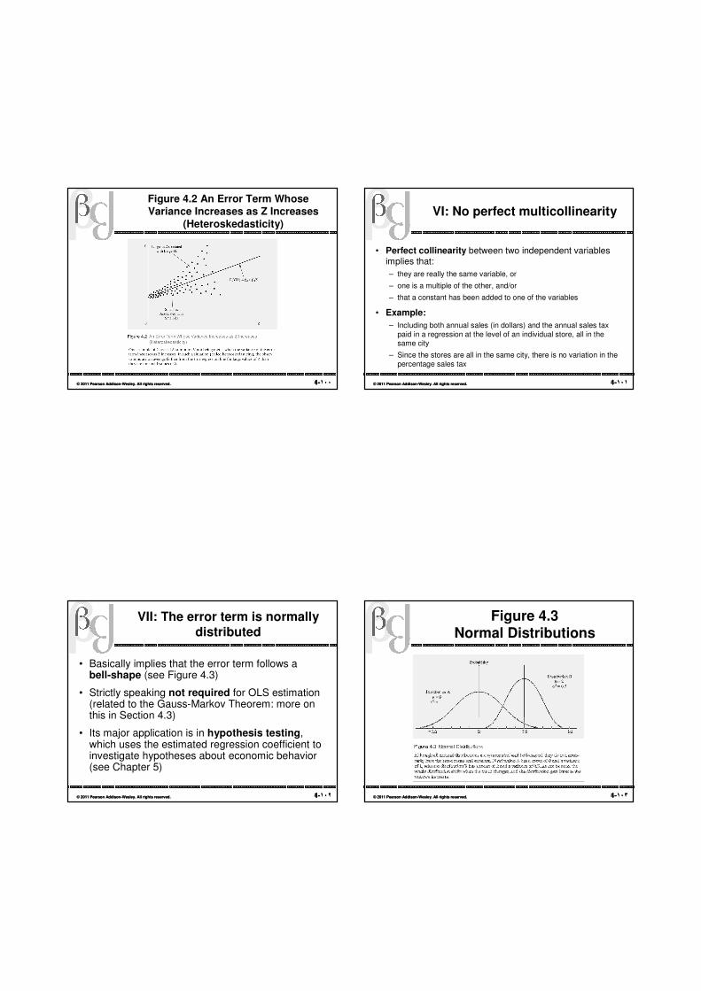
VII: The error term is normally distributed

• Basically implies that the error term follows a bell-shape (see Figure 4.3)

• Strictly speaking not required for OLS estimation (related to the Gauss-Markov Theorem: more on this in Section 4.3)

• Its major application is in hypothesis testing, which uses the estimated regression coefficient to investigate hypotheses about economic behavior (see Chapter 5)

1-١٠٣© 2011 Pearson Addison-Wesley. All rights reserved. 4-١٠٣© 2011 Pearson Addison-Wesley. All rights reserved.

Figure 4.3 Normal Distributions

1-١٠٤© 2011 Pearson Addison-Wesley. All rights reserved. 4-١٠٤© 2011 Pearson Addison-Wesley. All rights reserved.

The Sampling Distribution of

• We saw earlier that the error term follows a probability distribution (Classical Assumption VII)

• But so do the estimates of β!

– The probability distribution of these values across different samples is called the sampling distribution of

• We will now look at the properties of the mean, the variance, and the standard error of this sampling distribution

1-١٠٥© 2011 Pearson Addison-Wesley. All rights reserved. 4-١٠٥© 2011 Pearson Addison-Wesley. All rights reserved.

Properties of the Mean

• A desirable property of a distribution of estimates in that its mean equals the true mean of the variables being estimated

• Formally, an estimator is an unbiased estimator if its sampling distribution has as its expected value the true value of .

• We also write this as follows:

(4.9)

• Similarly, if this is not the case, we say that the estimator isbiased

1-١٠٦© 2011 Pearson Addison-Wesley. All rights reserved. 4-١٠٦© 2011 Pearson Addison-Wesley. All rights reserved.

Properties of the Variance

• Just as we wanted the mean of the sampling distribution to be centered around the true population , so too it is desirable for the sampling distribution to be as narrow (or precise) as possible.

– Centering around “the truth” but with high variability might be of very little use.

• One way of narrowing the sampling distribution is to increase the sampling size (which therefore also increases the degrees of freedom)

• These points are illustrated in Figures 4.4 and 4.5

1-١٠٧© 2011 Pearson Addison-Wesley. All rights reserved. 4-١٠٧© 2011 Pearson Addison-Wesley. All rights reserved.

Figure 4.4Distributions of

1-١٠٨© 2011 Pearson Addison-Wesley. All rights reserved. 4-١٠٨© 2011 Pearson Addison-Wesley. All rights reserved.

Figure 4.5 Sampling Distribution of for Various Observations (N)

1-١٠٩© 2011 Pearson Addison-Wesley. All rights reserved. 4-١٠٩© 2011 Pearson Addison-Wesley. All rights reserved.

Properties of the Standard Error

• The standard error of the estimated coefficient, SE( ), is the square root of the estimated variance of the estimated coefficients.

• Hence, it is similarly affected by the sample size and the other factors discussed previously

– For example, an increase in the sample size will decrease the standard error

– Similarly, the larger the sample, the more precise the coefficient estimates will be

1-١١٠© 2011 Pearson Addison-Wesley. All rights reserved. 4-١١٠© 2011 Pearson Addison-Wesley. All rights reserved.

The Gauss-Markov Theorem and the Properties of OLS Estimators

• The Gauss-Markov Theorem states that:

– Given Classical Assumptions I through VI (Assumption VII, normality, is not needed for this theorem), the Ordinary Least Squares estimator of –k is the minimum variance estimator from among the set of all linear unbiased estimators of –k, for k = 0, 1, 2, …, K

• We also say that “OLS is BLUE”: “Best (meaning minimum variance) Linear Unbiased Estimator”

1-١١١© 2011 Pearson Addison-Wesley. All rights reserved. 4-١١١© 2011 Pearson Addison-Wesley. All rights reserved.

The Gauss-Markov Theorem and the Properties of OLS Estimators (cont.)

• The Gauss-Markov Theorem only requires the first six classical assumptions

• If we add the seventh condition, normality, the OLS coefficient estimators can be shown to have the following properties:

– Unbiased: the OLS estimates coefficients are centered around the true population values

– Minimum variance: no other unbiased estimator has a lower variance for each estimated coefficient than OLS

– Consistent: as the sample size gets larger, the variance gets smaller, andeach estimate approaches the true value of the coefficient being estimated

– Normally distributed: when the error term is normally distributed, so are the estimated coefficients—which enables various statistical tests requiring normality to be applied (we’ll get back to this in Chapter 5)

1-١١٢© 2011 Pearson Addison-Wesley. All rights reserved. 4-١١٢© 2011 Pearson Addison-Wesley. All rights reserved.

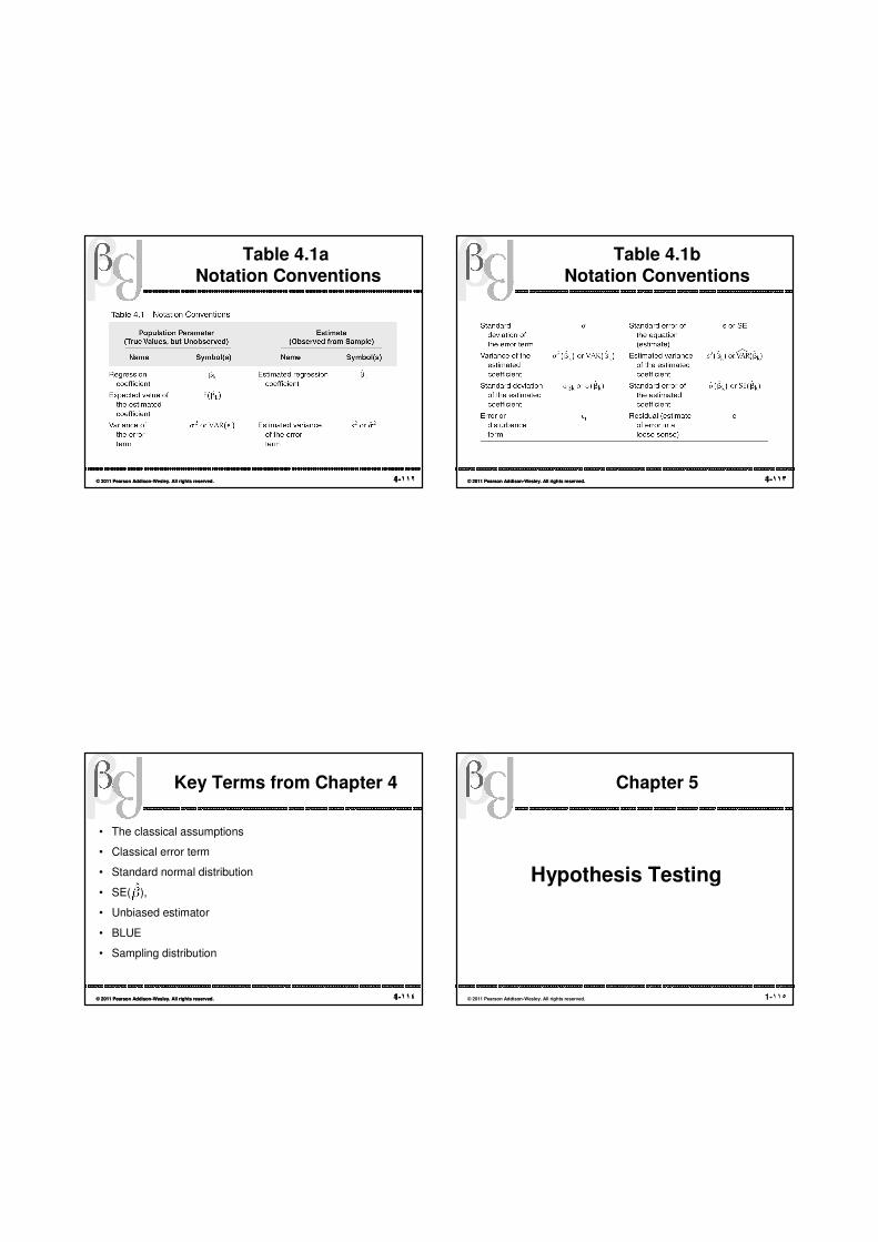
Table 4.1aNotation Conventions

1-١١٣© 2011 Pearson Addison-Wesley. All rights reserved. 4-١١٣© 2011 Pearson Addison-Wesley. All rights reserved.

Table 4.1bNotation Conventions

1-١١٤© 2011 Pearson Addison-Wesley. All rights reserved. 4-١١٤© 2011 Pearson Addison-Wesley. All rights reserved.


• The classical assumptions

• Classical error term

• Standard normal distribution

• SE( ),

• Unbiased estimator

• BLUE

• Sampling distribution

1-١١٥© 2011 Pearson Addison-Wesley. All rights reserved.

Chapter 5

Hypothesis Testing

1-١١٦© 2011 Pearson Addison-Wesley. All rights reserved.

What Is Hypothesis Testing?

• Hypothesis testing is used in a variety of settings

– The Food and Drug Administration (FDA), for example, tests new products before allowing their sale

• If the sample of people exposed to the new product shows some side effect significantly more frequently than would be expected to occur by chance, the FDA is likely to withhold approval of marketing that product

– Similarly, economists have been statistically testing various relationships, for example that between consumption and income

• Note here that while we cannot prove a given hypothesis (for example the existence of a given relationship), we often can reject a given hypothesis (again, for example, rejecting the existence of a given relationship)

1-١١٧© 2011 Pearson Addison-Wesley. All rights reserved.

Classical Null and Alternative Hypotheses

• The researcher first states the hypotheses to be tested

• Here, we distinguish between the null and the alternativehypothesis:

– Null hypothesis (“H0”): the outcome that the researcher does not

expect (almost always includes an equality sign)

– Alternative hypothesis (“HA”): the outcome the researcher doesexpect

• Example:

H0: β ≤ 0 (the values you do not expect)

HA: β > 0 (the values you do expect)

1-١١٨© 2011 Pearson Addison-Wesley. All rights reserved.

Type I and Type II Errors

• Two types of errors possible in hypothesis testing:

– Type I: Rejecting a true null hypothesis

– Type II: Not rejecting a false null hypothesis

• Example: Suppose we have the following null and alternative hypotheses:

H0: β ≤ 0

HA: β > 0

– Even if the trueβ really is not positive, in any one sample we might still observe an estimate of β that is sufficiently positive to lead to the rejection of the null hypothesis


1-١١٩© 2011 Pearson Addison-Wesley. All rights reserved.

Figure 5.1 Rejecting a True Null Hypothesis Is a Type I Error

1-١٢٠© 2011 Pearson Addison-Wesley. All rights reserved.

Type I and Type II Errors (cont.)

• Alternatively, it’s possible to obtain an estimate of β that is close enough to zero (or negative) to be considered “not significantly positive”

• Such a result may lead the researcher to “accept” the null hypothesis that β ≤ 0 when in truth β > 0

• This is a Type II Error; we have failed to reject a false null hypothesis!


1-١٢١© 2011 Pearson Addison-Wesley. All rights reserved.

Figure 5.2 Failure to Reject a False Null Hypothesis Is a Type II Error

1-١٢٢© 2011 Pearson Addison-Wesley. All rights reserved.

Decision Rules of Hypothesis Testing

• To test a hypothesis, we calculate a sample statistic that determines when the null hypothesis can be rejected depending on the magnitude of that sample statistic relative to a preselected critical value (which is found in a statistical table)

• This procedure is referred to as a decision rule

• The decision rule is formulated before regression estimates are obtained

• The range of possible values of the estimates is divided into two regions, an “acceptance” (really, non-rejection) region and a rejection region

• The critical value effectively separates the “acceptance”/non-rejection region from the rejection region when testing a null hypothesis

• Graphs of these “acceptance” and rejection regions are given in Figures 5.3 and 5.4

1-١٢٣© 2011 Pearson Addison-Wesley. All rights reserved.

Figure 5.3 “Acceptance” and Rejection Regions for a One-Sided Test of ββββ

1-١٢٤© 2011 Pearson Addison-Wesley. All rights reserved.

Figure 5.4 “Acceptance” and Rejection Regions for a Two-Sided Test of ββββ

1-١٢٥© 2011 Pearson Addison-Wesley. All rights reserved.

The t-Test

• The t-test is the test that econometricians usually use to test hypotheses about individual regression slope coefficients

– Tests of more than one coefficient at a time (joint hypotheses) are typically done with the F-test, presented in Section 5.6

• The appropriate test to use when the stochastic error term is normally distributed and when the variance of that distribution must be estimated

– Since these usually are the case, the use of the t-test for hypothesis testing has become standard practice in econometrics

1-١٢٦© 2011 Pearson Addison-Wesley. All rights reserved.

The t-Statistic

• For a typical multiple regression equation:

(5.1)

we can calculate t-values for each of the estimated coefficients

– Usually these are only calculated for the slope coefficients, though (see Section 7.1)

• Specifically, the t-statistic for the kth coefficient is:

(5.2)

1-١٢٧© 2011 Pearson Addison-Wesley. All rights reserved.

The Critical t-Value and the t-Test Decision Rule

• To decide whether to reject or not to reject a null hypothesis based on a calculated t-value, we use a critical t-value

• A critical t-value is the value that distinguishes the “acceptance”region from the rejection region

• The critical t-value, tc, is selected from a t-table (see Statistical Table B-1 in the back of the book) depending on:

– whether the test is one-sided or two-sided,

– the level of Type I Error specified and

– the degrees of freedom (defined as the number of observations minus the number of coefficients estimated (including the constant) or N – K – 1)

1-١٢٨© 2011 Pearson Addison-Wesley. All rights reserved.

The Critical t-Value and the t-Test Decision Rule (cont.)

• The rule to apply when testing a single regression coefficient ends up being that you should:

Reject H0 if |tk| > tc and if tk also has the sign implied by HA

Do not reject H0 otherwise

1-١٢٩© 2011 Pearson Addison-Wesley. All rights reserved.


• Note that this decision rule works both for calculated t-values and critical t-values for one-sided hypotheses around zero (or another hypothesized value, S):

H0: βk ≤ 0 H0: βk ≤ S

HA: βk > 0 HA: βk > S

H0: βk ≥ 0 H0: βk ≥ S

HA: βk < 0 HA: βk < S

1-١٣٠© 2011 Pearson Addison-Wesley. All rights reserved.


• As well as for two-sided hypotheses around zero (or another hypothesized value, S):

H0: βk = 0 H0: βk = S

HA: βk ≠ 0 HA: βk ≠ S

• From Statistical Table B-1 the critical t-value for a one-tailed test at a given level of significance is exactly equal to the critical t-value for a two-tailed test at twice the level of significance of the one-tailed test—as also illustrated by Figure 5.5

1-١٣١© 2011 Pearson Addison-Wesley. All rights reserved.

Figure 5.5 One-Sided and Two-Sided t-Tests

1-١٣٢© 2011 Pearson Addison-Wesley. All rights reserved.

Choosing a Level of Significance

• The level of significance must be chosen before a critical value can be found, using Statistical Table B

• The level of significance indicates the probability of observing an estimated t-value greater than the criticalt-value if the null hypothesis were correct

• It also measures the amount of Type I Error implied by a particular critical t-value

• Which level of significance is chosen?

– 5 percent is recommended, unless you know something unusual about the relative costs of making Type I and Type II Errors

1-١٣٣© 2011 Pearson Addison-Wesley. All rights reserved.

Confidence Intervals

• A confidence interval is a range that contains the true value of an item a specified percentage of the time

• It is calculated using the estimated regression coefficient, thetwo-sided critical t-value and the standard error of the estimated coefficient as follows:

(5.5)

• What’s the relationship between confidence intervals and two-sided hypothesis testing?

• If a hypothesized value fall within the confidence interval, then we cannot reject the null hypothesis

1-١٣٤© 2011 Pearson Addison-Wesley. All rights reserved.

p-Values

• This is an alternative to the t-test

• A p-value, or marginal significance level, is the probability of observing a t-score that size or larger (in absolute value) if the null hypothesiswere true

• Graphically, it’s two times the area under the curve of the t-distribution between the absolute value of the actual t-score and infinity.

• In theory, we could find this by combing through pages and pages of statistical tables

• But we don’t have to, since we have EViews and Stata: these (and other) statistical software packages automatically give thep-values as part of the standard output!

• In light of all this, the p-value decision rule therefore is:

Reject H0 if p-valueK < the level of significance and if has the sign implied by HA

1-١٣٥© 2011 Pearson Addison-Wesley. All rights reserved.

Examples of t-Tests: One-Sided

• The most common use of the one-sided t-test is to determine whether a regression coefficient is significantly different from zero (in the direction predicted by theory!)

• This involves four steps:

1. Set up the null and alternative hypothesis

2. Choose a level of significance and therefore a critical t-value

3. Run the regression and obtain an estimated t-value (or t-score)

4. Apply the decision rule by comparing calculated t-value with thecritical t-value in order to reject or not reject the null hypothesis

• Let’s look at each step in more detail for a specific example:

1-١٣٦© 2011 Pearson Addison-Wesley. All rights reserved.

Examples of t-Tests: One-Sided (cont.)

• Consider the following simple model of the aggregate retail sales of new cars:

(5.6)

Where:

Y = sales of new cars

X1 = real disposable income

X2 = average retail price of a new car adjusted by the consumer price index

X3 = number of sports utility vehicles sold

• The four steps for this example then are as follows:

1-١٣٧© 2011 Pearson Addison-Wesley. All rights reserved.

Step 1: Set up the null and alternative hypotheses

• From equation 5.6, the one-sided hypotheses are set up as:

1. H0: β1 ≤ 0HA: β1 > 0

2. H0: β2 ≥ 0 HA: β2 < 0

3. H0: β3 ≥ 0HA: β3 < 0

• Remember that a t-test typically is not run on the estimate of the constant termβ0

1-١٣٨© 2011 Pearson Addison-Wesley. All rights reserved.

Step 2: Choose a level of significance and therefore a critical t-value

• Assume that you have considered the various costs involved in making Type I and Type II Errors and have chosen 5 percent as the level of significance

• There are 10 observations in the data set, and so there are 10 – 3 – 1 = 6 degrees of freedom

• At a 5-percent level of significance, the critical t-value, tc, can be found in Statistical Table B-1 to be 1.943

1-١٣٩© 2011 Pearson Addison-Wesley. All rights reserved.

Step 3: Run the regression and obtain an estimated t-value

• Use the data (annual from 2000 to 2009) to run the regression on your OLS computer package

• Again, most statistical software packages automatically report the t-values

• Assume that in this case the t-values were 2.1, 5.6, and –0.1 for β1, β2, and β3, respectively

1-١٤٠© 2011 Pearson Addison-Wesley. All rights reserved.

Step 4: Apply the t–test decision rule

• As stated in Section 5.2, the decision rule for the t-test is to:

Reject H0 if |tk| > tc and if tk also has the sign implied by HA

• In this example, this amounts to the following three conditions:

For β1: Reject H0 if |2.1| > 1.943 and if 2.1 is positive.

For β2: Reject H0 if |5.6| > 1.943 and if 5.6 is positive.

For β3: Reject H0 if |–0.1| > 1.943 and if –0.1 is positive.

• Figure 5.6 illustrates all three of these outcomes

1-١٤١© 2011 Pearson Addison-Wesley. All rights reserved.

Figure 5.6a One-Sided t-Tests of the Coefficients of the New Car Sales Model

1-١٤٢© 2011 Pearson Addison-Wesley. All rights reserved.

Figure 5.6b One-Sided t-Tests of the Coefficients of the New Car Sales Model

1-١٤٣© 2011 Pearson Addison-Wesley. All rights reserved.

Examples of t-Tests: Two-Sided

• The two-sided test is used when the hypotheses should be rejected if estimated coefficients are significantly different from zero, or a specific nonzero value, in either direction

• So, there are two cases:

1. Two-sided tests of whether an estimated coefficient is significantly different from zero, and

2. Two-sided tests of whether an estimated coefficient is significantly different from a specific nonzero value

• Let’s take an example to illustrate the first of these (the second case is merely a generalized case of this, see the textbook for details), using the Woody’s restaurant example in Chapter 3:

1-١٤٤© 2011 Pearson Addison-Wesley. All rights reserved.

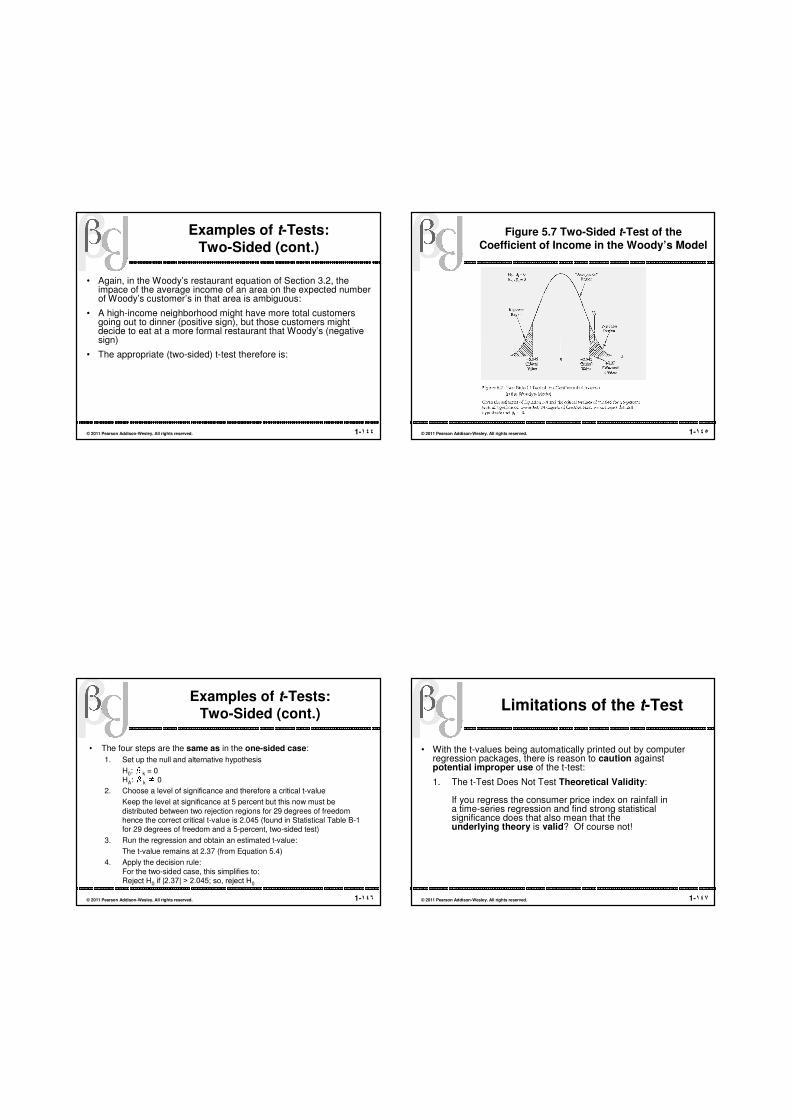
Examples of t-Tests: Two-Sided (cont.)

• Again, in the Woody’s restaurant equation of Section 3.2, the impace of the average income of an area on the expected number of Woody’s customer’s in that area is ambiguous:

• A high-income neighborhood might have more total customers going out to dinner (positive sign), but those customers might decide to eat at a more formal restaurant that Woody’s (negative sign)

• The appropriate (two-sided) t-test therefore is:

1-١٤٥© 2011 Pearson Addison-Wesley. All rights reserved.

Figure 5.7 Two-Sided t-Test of the Coefficient of Income in the Woody’s Model

1-١٤٦© 2011 Pearson Addison-Wesley. All rights reserved.

Examples of t-Tests: Two-Sided (cont.)

• The four steps are the same as in the one-sided case:

1. Set up the null and alternative hypothesis

H0: βk = 0HA: βk≠ 0

2. Choose a level of significance and therefore a critical t-value

Keep the level at significance at 5 percent but this now must bedistributed between two rejection regions for 29 degrees of freedom hence the correct critical t-value is 2.045 (found in Statistical Table B-1 for 29 degrees of freedom and a 5-percent, two-sided test)

3. Run the regression and obtain an estimated t-value:

The t-value remains at 2.37 (from Equation 5.4)

4. Apply the decision rule:For the two-sided case, this simplifies to:Reject H0 if |2.37| > 2.045; so, reject H0

1-١٤٧© 2011 Pearson Addison-Wesley. All rights reserved.

Limitations of the t-Test

• With the t-values being automatically printed out by computer regression packages, there is reason to caution against potential improper use of the t-test:

1. The t-Test Does Not Test Theoretical Validity:

If you regress the consumer price index on rainfall ina time-series regression and find strong statistical significance does that also mean that the underlying theory is valid? Of course not!

1-١٤٨© 2011 Pearson Addison-Wesley. All rights reserved.

Limitations of the t-Test

2. The t-Test Does Not Test “Importance”:

The fact that one coefficient is “more statistically significant” than another does not mean that it is also more important in explaining the dependent variable—but merely that we have more evidenceof the sign of the coefficient in question

3. The t-Test Is Not Intended for Tests of the Entire Population:

From the definition of the t-score, given by Equation5.2, it is seen that as the sample size approaches the population (whereby the standard error will approach zero—since the standard error decreases as N increases), the t-score will approach infinity!

1-١٤٩© 2011 Pearson Addison-Wesley. All rights reserved.

The F-Test of Overall Significance

We can test for the predictive power of the entire model using the F statistic

• Generally these compare two sources of variation

• F = V1/V2 and has two df parameters

• Here V1 = ESS/K has K df

• And V2 = RSS/(n-K-1) has n-K-1 df

Usually will see several pages of these; one or two pages at

each specific level of significance (.10, .05, .01).

Value of F at a

specific significance level

Numerator d.f.

denom.

d.f.

F Tables F Test Hypotheses

H0: β1 = β2 = …= βK = 0 (None of the Xs help explain Y)

Ha: Not all βs are 0 (At least one X is useful)

H0: R2 = 0 is an equivalent hypothesis

Reject H0 if F≥Fc

Do Not Reject H0 if F<Fc

The critical F-value, Fc, is determined from Statistical Tables

B-2 or B3 depending on a level of significance, αααα, and degrees

of freedom, df1=K , (K, the number of the independent

variables) and df2=n-k-1

Example: The Woody's restaurant

• Since there are 3 independent variables, the null and alternative hypotheses are:

H0: ββββN = ββββP = ββββI = 0

Ha: Not all ββββs are 0

• From E-Views output, F=15.65, Fc(0.05;3,29)=2.93

• Fc is well below the calculated F-value of 15.65, so we can rejectthe null hypothesis and conclude that the Woody's equation does indeed have a significance of overall fit.

1-١٥٣© 2011 Pearson Addison-Wesley. All rights reserved.


• Null hypothesis

• Alternative hypothesis

• Type I Error

• Level of significance

• Two-sided test

• Decision rule

• Critical value

• t-statistic

• Confidence interval

• p-value

1-١٥٤© 2011 Pearson Addison-Wesley. All rights reserved.

Chapter 6

Model Specification: Choosing the Independent Variables

1-١٥٥© 2011 Pearson Addison-Wesley. All rights reserved.

Specifying an Econometric Equation and Specification Error

• Before any equation can be estimated, it must be completely specified

• Specifying an econometric equation consists of three parts, namely choosing the correct:

– independent variables

– functional form

– form of the stochastic error term

• Again, this is part of the first classical assumption from Chapter 4

• A specification error results when one of these choices is made incorrectly

• This chapter will deal with the first of these choices (the two other choices will be discussed in subsequent chapters)

1-١٥٦© 2011 Pearson Addison-Wesley. All rights reserved.

Omitted Variables

• Two reasons why an important explanatory variable might have been left out:

– we forgot…

– it is not available in the dataset, we are examining

• Either way, this may lead to omitted variable bias(or, more generally, specification bias)

• The reason for this is that when a variable is not included, it cannot be held constant

• Omitting a relevant variable usually is evidence that the entire equation is a suspect, because of the likely bias of the coefficients.

1-١٥٧© 2011 Pearson Addison-Wesley. All rights reserved.

The Consequences of an Omitted Variable

• Suppose the true regression model is:

(6.1)

Where is a classical error term

• If X2 is omitted, the equation becomes instead:

(6.2)

Where:

(6.3)

• Hence, the explanatory variables in the estimated regression (6.2) are not

independent of the error term (unless the omitted variable is uncorrelatedwith all the included variables—something which is very unlikely)

• But this violates Classical Assumption III!

1-١٥٨© 2011 Pearson Addison-Wesley. All rights reserved.

The Consequences of an Omitted Variable (cont.)

• What happens if we estimate Equation 6.2 when Equation 6.1 is the truth?

• We get bias!

• What this means is that:

(6.4)

• The amount of bias is a function of the impact of the omitted variable on the dependent variable times a function of the correlation between the includedand the omitted variable

• Or, more formally:

(6.7)

• So, the bias exists unless:

1. the true coefficient equals zero, or

2. the included and omitted variables are uncorrelated

1-١٥٩© 2011 Pearson Addison-Wesley. All rights reserved.

Correcting for an Omitted Variable

• In theory, the solution to a problem of specification bias seems easy: add the omitted variable to the equation!

• Unfortunately, that’s easier said than done, for a couple of reasons

1. Omitted variable bias is hard to detect: the amount of bias introduced can be small and not immediately detectable

2. Even if it has been decided that a given equation is suffering from omitted variable bias, how to decide exactly which variable to include?

• Note here that dropping a variable is not a viable strategy to help cure omitted variable bias:

– If anything you’ll just generate even more omitted variable bias on the remaining coefficients!

1-١٦٠© 2011 Pearson Addison-Wesley. All rights reserved.

Correcting for an Omitted Variable (cont.)

• What if:

– You have an unexpected result, which leads you to believe that you have an omitted variable

– You have two or more theoretically sound explanatory variables as potential “candidates” for inclusion as the omitted variable to the equation is to use

• How do you choose between these variables?

• One possibility is expected bias analysis

– Expected bias: the likely bias that omitting a particular variable would have caused in the estimated coefficient of one of the included variables

1-١٦١© 2011 Pearson Addison-Wesley. All rights reserved.

Correcting for an Omitted Variable (cont.)

• Expected bias can be estimated with Equation 6.7:

(6.7)

• When do we have a viable candidate?

– When the sign of the expected bias is the same as the signof the unexpected result

• Similarly, when these signs differ, the variable is extremely unlikely to have caused the unexpected result

1-١٦٢© 2011 Pearson Addison-Wesley. All rights reserved.

Irrelevant Variables

• This refers to the case of including a variable in an equation when it does not belong there

• This is the opposite of the omitted variables case—and so the impact can be illustrated using the same model

• Assume that the true regression specification is:

(6.10)

• But the researcher for some reason includes an extra variable:

(6.11)

• The misspecified equation’s error term then becomes:

(6.12)

1-١٦٣© 2011 Pearson Addison-Wesley. All rights reserved.

Irrelevant Variables (cont.)

• So, the inclusion of an irrelevant variable will not cause bias

(since the true coefficient of the irrelevant variable is zero, and so the second term will drop out of Equation 6.12)

• However, the inclusion of an irrelevant variable will:

– Increase the variance of the estimated coefficients, and this increased variance will tend to decrease the absolute magnitude of their t-scores

– Decrease the R2 (but not the R2)

• Table 6.1 summarizes the consequences of the omitted variable and the included irrelevant variable cases (unless r12 = 0)

1-١٦٤© 2011 Pearson Addison-Wesley. All rights reserved.

Table 6.1 Effect of Omitted Variables and Irrelevant Variables on the Coefficient Estimates

1-١٦٥© 2011 Pearson Addison-Wesley. All rights reserved.

Four Important Specification Criteria

• We can summarize the previous discussion into four criteria to help decide whether a given variable belongs in the equation:

1. Theory: Is the variable’s place in the equation unambiguous and theoretically sound?

2. t-Test: Is the variable’s estimated coefficient significant in the expected direction?

3. R2: Does the overall fit of the equation (adjusted for degrees of freedom) improve when the variable is added to the equation?

4. Bias: Do other variables’ coefficients change significantly when the variable is added to the equation?

• If all these conditions hold, the variable belongs in the equation

• If none of them hold, it does not belong

• The tricky part is the intermediate cases: use sound judgment!

1-١٦٦© 2011 Pearson Addison-Wesley. All rights reserved.

Specification Searches

• Almost any result can be obtained from a given dataset, by simply specifying different regressions until estimates with the desired properties are obtained

• Hence, the integrity of all empirical work is open to question

• To counter this, the following three points of Best Practices in Specification Searches are suggested:

1. Rely on theory rather than statistical fit as much as possible when choosing variables, functional forms, and the like

2. Minimize the number of equations estimated (except for sensitivity analysis, to be discussed later in this section)

3. Reveal, in a footnote or appendix, all alternative specifications estimated

1-١٦٧© 2011 Pearson Addison-Wesley. All rights reserved.

Sequential Specification Searches

• The sequential specification search technique allows a researcher to:

– Estimate an undisclosed number of regressions

– Subsequently present a final choice (which is based upon an unspecified set of expectations about the signs and significance of the coefficients) as if it were only a specification

• Such a method misstates the statistical validity of the regression results for two reasons:

1. The statistical significance of the results is overestimated because the estimations of the previous regressions are ignored

2. The expectations used by the researcher to choose between various regression results rarely, if ever, are disclosed

1-١٦٨© 2011 Pearson Addison-Wesley. All rights reserved.

Bias Caused by Relying on the t-Test to Choose Variables

• Dropping variables solely based on low t-statistics may lead to two different types of errors:

1. An irrelevant explanatory variable may sometimes be included in the equation (i.e., when it does not belong there)

2. A relevant explanatory variables may sometimes be dropped from the equation (i.e., when it does belong)

• In the first case, there is no bias but in the second case there is bias

• Hence, the estimated coefficients will be biased every time an excludedvariable belongs in the equation, and that excluded variable will be left outevery time its estimated coefficient is not statistically significantly different from zero

• So, we will have systematic bias in our equation!

1-١٦٩© 2011 Pearson Addison-Wesley. All rights reserved.

Sensitivity Analysis

• Contrary to the advice of estimating as few equations as possible

(and based on theory, rather than fit!), sometimes we see journal article authors listing results from five or more specifications

• What’s going on here:

• In almost every case, these authors have employed a technique called sensitivity analysis

• This essentially consists of purposely running a number of alternative specifications to determine whether particular results are robust (not statistical flukes) to a change in specification

• Why is this useful? Because true specification isn’t known!

1-١٧٠© 2011 Pearson Addison-Wesley. All rights reserved.

Data Mining

• Data mining involves exploring a data set to try to uncover empirical regularities that can inform economic theory

• That is, the role of data mining is opposite that of traditionaleconometrics, which instead tests the economic theory on a data set

• Be careful, however!

– a hypothesis developed using data mining techniques must be tested on a different data set (or in a different context) than the one used to develop the hypothesis

– Not doing so would be highly unethical: After all, the researcher already knows ahead of time what the results will be!

1-١٧١© 2011 Pearson Addison-Wesley. All rights reserved.


• Omitted variable

• Irrelevant variable

• Specification bias

• Sequential specification search

• Specification error

• The four specification criteria

• Expected bias

• Sensitivity analysis

1-١٧٢© 2011 Pearson Addison-Wesley. All rights reserved.

Chapter 7

Model Specification: Choosing a Functional Form

1-١٧٣© 2011 Pearson Addison-Wesley. All rights reserved.

The Use and Interpretation of the Constant Term

• An estimate of β0 has at least three components:

1. the true β0

2. the constant impact of any specification errors (an omitted variable, for example)

3. the mean of ε for the correctly specified equation (if not equal to zero)

• Unfortunately, these components can’t be distinguished from one another because we can observe only β0, the sum of the three components

• As a result of this, we usually don’t interpret the constant term

• On the other hand, we should not suppress the constant term, either, as illustrated by Figure 7.1

1-١٧٤© 2011 Pearson Addison-Wesley. All rights reserved.

Figure 7.1 The Harmful Effect of Suppressing the Constant Term

1-١٧٥© 2011 Pearson Addison-Wesley. All rights reserved.

Alternative Functional Forms

• An equation is linear in the variables if plotting the function in terms of X and Y generates a straight line

• For example, Equation 7.1:

Y = β0 + β1X + ε (7.1)

is linear in the variables but Equation 7.2:

Y = β0 + β1X2 + ε (7.2)

is not linear in the variables

• Similarly, an equation is linear in the coefficients only if the coefficients

appear in their simplest form—they:

– are not raised to any powers (other than one)

– are not multiplied or divided by other coefficients

– do not themselves include some sort of function (like logs or exponents)

1-١٧٦© 2011 Pearson Addison-Wesley. All rights reserved.

• For example, Equations 7.1 and 7.2 are linear in the coefficients, while Equation 7:3:

(7.3)

is not linear in the coefficients

• In fact, of all possible equations for a single explanatory variable, only functions of the general form:

(7.4)

are linear in the coefficients β0 and β1

Alternative Functional Forms (cont.)

1-١٧٧© 2011 Pearson Addison-Wesley. All rights reserved.

Linear Form

• This is based on the assumption that the slope of the relationship between the independent variable and the dependent variable is constant:

• For the linear case, the elasticity of Y with respect to X (the percentage change in the dependent variable caused by a 1-percent increase in the independent variable, holding the other variables in the equation constant) is:

1-١٧٨© 2011 Pearson Addison-Wesley. All rights reserved.

What Is a Log?

• If e (a constant equal to 2.71828) to the “bth power” produces x, then b is the log of x:

b is the log of x to the base e if: eb = x

• Thus, a log (or logarithm) is the exponent to which a given base must be taken in order to produce a specific number

• While logs come in more than one variety, we’ll use only natural logs (logs to the base e) in this text

• The symbol for a natural log is “ln,” so ln(x) = b means that (2.71828) b = x or, more simply,

ln(x) = b means that eb = x

• For example, since e2 = (2.71828) 2 = 7.389, we can state that:

ln(7.389) = 2

Thus, the natural log of 7.389 is 2! Again, why? Two is the power of e that produces 7.389

1-١٧٩© 2011 Pearson Addison-Wesley. All rights reserved.

What Is a Log? (cont.)

• Let’s look at some other natural log calculations:

ln(100) = 4.605

ln(1000) = 6.908

ln(10000) = 9.210

ln(1000000) = 13.816

n(100000) = 11.513

• Note that as a number goes from 100 to 1,000,000, its natural log goes from 4.605 to only 13.816! As a result, logs can be used in econometrics if a researcher wants to reduce the absolute size of the numbers associated with the same actual meaning

• One useful property of natural logs in econometrics is that they make it easier to figure out impacts in percentage terms (we’ll see this when we get to the double-

log specification)

1-١٨٠© 2011 Pearson Addison-Wesley. All rights reserved.

Double-Log Form

• Here, the natural log of Y is the dependent variable and the natural log of X is the independent variable:

(7.5)

• In a double-log equation, an individual regression coefficient can be interpreted as an elasticity because:

(7.6)

• Note that the elasticities of the model are constant and the slopes are not

• This is in contrast to the linear model, in which the slopes are constant but the elasticities are not

1-١٨١© 2011 Pearson Addison-Wesley. All rights reserved.

Figure 7.2 Double-Log Functions

1-١٨٢© 2011 Pearson Addison-Wesley. All rights reserved.

Semilog Form

• The semilog functional form is a variant of the double-log equation in which some but not all of the variables (dependent and independent) are expressed in terms of their natural logs.

• It can be on the right-hand side, as in:

Yi = β0 + β1lnX1i + β2X2i + εi (7.7)

• Or it can be on the left-hand side, as in:

lnY = β0 + β1X1 + β2X2 + ε (7.9)

• Figure 7.3 illustrates these two different cases

1-١٨٣© 2011 Pearson Addison-Wesley. All rights reserved.

Figure 7.3 Semilog Functions

1-١٨٤© 2011 Pearson Addison-Wesley. All rights reserved.

Polynomial Form

• Polynomial functional forms express Y as a function of independent variables, some of which are raised to powers other than 1

• For example, in a second-degree polynomial (also called a quadratic) equation, at least one independent variable is squared:

Yi = β0 + β1X1i + β2(X1i)2 + β3X2i + εi (7.10)

• The slope of Y with respect to X1 in Equation 7.10 is:

(7.11)

• Note that the slope depends on the level of X1

1-١٨٥© 2011 Pearson Addison-Wesley. All rights reserved.

Figure 7.4 Polynomial Functions

1-١٨٦© 2011 Pearson Addison-Wesley. All rights reserved.

Inverse Form

• The inverse functional form expresses Y as a function of the reciprocal (or inverse) of one or more of the independent variables (in this case, X1):

Yi = β0 + β1(1/X1i) + β2X2i + εi (7.13)

• So X1 cannot equal zero

• This functional form is relevant when the impact of a particularindependent variable is expected to approach zero as that independent variable approaches infinity

• The slope with respect to X1 is:

(7.14)

• The slopes for X1 fall into two categories, depending on the sign of β1 (illustrated in Figure 7.5)

1-١٨٧© 2011 Pearson Addison-Wesley. All rights reserved.

Figure 7.5 Inverse Functions

1-١٨٨© 2011 Pearson Addison-Wesley. All rights reserved.

Table 7.1 Summary of Alternative Functional Forms

1-١٨٩© 2011 Pearson Addison-Wesley. All rights reserved.

Lagged Independent Variables

• Virtually all the regressions we’ve studied so far have been “instantaneous” in nature

• In other words, they have included independent and dependent variables from the same time period, as in:

Yt = β0 + β1X1t + β2X2t + εt (7.15)

• Many econometric equations include one or more lagged independent variables like X1t-1 where “t–1” indicates that the observation of X1 is from the time period previous to time period t, as in the following equation:

Yt = β0 + β1X1t-1 + β2X2t + εt (7.16)

1-١٩٠© 2011 Pearson Addison-Wesley. All rights reserved.

Using Dummy Variables

• A dummy variable is a variable that takes on the values of 0 or 1, depending on whether a condition for a qualitative attribute (such as gender) is met

• These conditions take the general form:

(7.18)

• This is an example of an intercept dummy (as opposed to a slope dummy, which is discussed in Section 7.5)

• Figure 7.6 illustrates the consequences of including an intercept dummy in a linear regression model

1-١٩١© 2011 Pearson Addison-Wesley. All rights reserved.

Figure 7.6 An Intercept Dummy

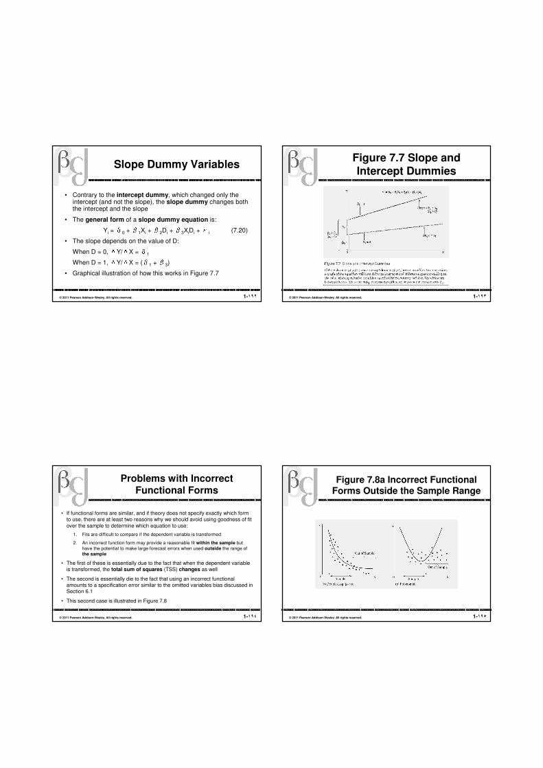
1-١٩٢© 2011 Pearson Addison-Wesley. All rights reserved.

Slope Dummy Variables

• Contrary to the intercept dummy, which changed only the intercept (and not the slope), the slope dummy changes both the intercept and the slope

• The general form of a slope dummy equation is:

Yi = β0 + β1Xi + β2Di + β3XiDi + εi (7.20)

• The slope depends on the value of D:

When D = 0, ΔY/ΔX = β1

When D = 1, ΔY/ΔX = (β1 + β3)

• Graphical illustration of how this works in Figure 7.7

1-١٩٣© 2011 Pearson Addison-Wesley. All rights reserved.

Figure 7.7 Slope and Intercept Dummies

1-١٩٤© 2011 Pearson Addison-Wesley. All rights reserved.

Problems with Incorrect Functional Forms

• If functional forms are similar, and if theory does not specify exactly which form to use, there are at least two reasons why we should avoid using goodness of fit over the sample to determine which equation to use:

1. Fits are difficult to compare if the dependent variable is transformed

2. An incorrect function form may provide a reasonable fit within the sample but have the potential to make large forecast errors when used outside the range of the sample

• The first of these is essentially due to the fact that when the dependent variable is transformed, the total sum of squares (TSS) changes as well

• The second is essentially die to the fact that using an incorrect functional amounts to a specification error similar to the omitted variables bias discussed in Section 6.1

• This second case is illustrated in Figure 7.8

1-١٩٥© 2011 Pearson Addison-Wesley. All rights reserved.

Figure 7.8a Incorrect Functional Forms Outside the Sample Range

1-١٩٦© 2011 Pearson Addison-Wesley. All rights reserved.

Figure 7.8b Incorrect Functional Forms Outside the Sample Range

1-١٩٧© 2011 Pearson Addison-Wesley. All rights reserved.


• Elasticity

• Double-log functional form

• Semilog functional form

• Polynomial functional form

• Inverse functional form

• Slope dummy

• Natural log

• Omitted condition

• Interaction term

• Linear in the variables

• Linear in the coefficients

1-١٩٨© 2011 Pearson Addison-Wesley. All rights reserved.

Chapter 8

Multicollinearity

1-١٩٩© 2011 Pearson Addison-Wesley. All rights reserved.

Introduction and Overview

• The next three chapters deal with violations of the Classical Assumptions and remedies for those violations

• This chapter addresses multicollinearity; the next two chapters are on serial correlation and heteroskedasticity

• For each of these three problems, we will attempt to answer the following questions:

1. What is the nature of the problem?

2. What are the consequences of the problem?

3. How is the problem diagnosed?

4. What remedies for the problem are available?

1-٢٠٠© 2011 Pearson Addison-Wesley. All rights reserved.

Perfect Multicollinearity

• Perfect multicollinearity violates Classical Assumption VI, which specifies that no explanatory variable is a perfect linear function of any other explanatory variables

• The word perfect in this context implies that the variation in one explanatory variable can be completely explained by movements in another explanatory variable

– A special case is that of a dominant variable: an explanatory variable is definitionally related to the dependent variable

• An example would be (Notice: no error term!):

X1i = α0 + α1X2i (8.1)

where the αs are constants and the Xs are independent variables in:

Yi = β0 + β1X1i + β2X2i + εi (8.2)

• Figure 8.1 illustrates this case

1-٢٠١© 2011 Pearson Addison-Wesley. All rights reserved.

Figure 8.1 Perfect Multicollinearity

1-٢٠٢© 2011 Pearson Addison-Wesley. All rights reserved.

Perfect Multicollinearity (cont.)

• What happens to the estimation of an econometric equation where there is perfect multicollinearity?

– OLS is incapable of generating estimates of the regression coefficients

– most OLS computer programs will print out an error message in such a situation

• What is going on?

• Essentially, perfect multicollinearity ruins our ability to estimate the coefficients because the perfectly collinear variables cannot be distinguished from each other:

• You cannot “hold all the other independent variables in the equation constant” if every time one variable changes, another changes in an identical manner!

• Solution: one of the collinear variables must be dropped (they are essentially identical, anyway)

1-٢٠٣© 2011 Pearson Addison-Wesley. All rights reserved.

Imperfect Multicollinearity

• Imperfect multicollinearity occurs when two (or more) explanatory variables are imperfectly linearly related, as in:

X1i = α0 + α1X2i + ui (8.7)

• Compare Equation 8.7 to Equation 8.1

– Notice that Equation 8.7 includes ui, a stochastic error term

• This case is illustrated in Figure 8.2

1-٢٠٤© 2011 Pearson Addison-Wesley. All rights reserved.

Figure 8.2 Imperfect Multicollinearity

1-٢٠٥© 2011 Pearson Addison-Wesley. All rights reserved.

The Consequences of Multicollinearity

There are five major consequences of multicollinearity:

1. Estimates will remain unbiased

2. The variances and standard errors of the estimates will increase:

a. Harder to distinguish the effect of one variable from the effect of another, so much more likely to make large errors in estimating the βs than without multicollinearity

b. As a result, the estimated coefficients, although still unbiased, now come from distributions with much larger variances and, therefore, larger standard errors (this point is illustrated in Figure 8.3)

1-٢٠٦© 2011 Pearson Addison-Wesley. All rights reserved.

Figure 8.3 Severe Multicollinearity

Increases the Variances of the s

1-٢٠٧© 2011 Pearson Addison-Wesley. All rights reserved.

The Consequences of Multicollinearity (cont.)

3. The computed t-scores will fall:

a. Recalling Equation 5.2, this is a direct consequence of 2. above

4. Estimates will become very sensitive to changes in specification:

a. The addition or deletion of an explanatory variable or of a few observations

will often cause major changes in the values of the s when significant multicollinearity exists

b. For example, if you drop a variable, even one that appears to be statistically insignificant, the coefficients of the remaining variables in the equation sometimes will change dramatically

c. This is again because with multicollinearity, it is much harder to distinguish

the effect of one variable from the effect of another

5. The overall fit of the equation and the estimation of the coefficients of nonmulticollinear variables will be largely unaffected

1-٢٠٨© 2011 Pearson Addison-Wesley. All rights reserved.

The Detection of Multicollinearity

• First realize that that some multicollinearity exists in every

equation: all variables are correlated to some degree (even if completely at random)

• So it’s really a question of how much multicollinearity exists in an equation, rather than whether any multicollinearity exists

• There are basically two characteristics that help detect the degree of multicollinearity for a given application:

1. High simple correlation coefficients

2. High Variance Inflation Factors (VIFs)

• We will now go through each of these in turn:

1-٢٠٩© 2011 Pearson Addison-Wesley. All rights reserved.

High Simple Correlation Coefficients

• If a simple correlation coefficient, r, between any two explanatory variables is high in absolute value, these two particular Xs are highly correlated and multicollinearity is a potential problem

• How high is high?

– Some researchers pick an arbitrary number, such as 0.80

– A better answer might be that r is high if it causes unacceptably large variances in the coefficient estimates in which we’re interested.

• Caution in case of more than two explanatory variables:

– Groups of independent variables, acting together, may cause multicollinearity without any single simple correlation coefficient being high enough to indicate that multicollinearity is present

– As a result, simple correlation coefficients must be considered to be sufficient but not necessary tests for multicollinearity

1-٢١٠© 2011 Pearson Addison-Wesley. All rights reserved.

High Variance Inflation Factors (VIFs)

The variance inflation factor (VIF) is calculated from two steps:

1. Run an OLS regression that has Xi as a function of all the other explanatory variables in the equation—For i = 1, this equation would be:

X1 = α1 + α2X2 + α3X3 + … + αKXK + v (8.15)

where v is a classical stochastic error term

2. Calculate the variance inflation factor for :

(8.16)

where is the unadjusted from step one

1-٢١١© 2011 Pearson Addison-Wesley. All rights reserved.

High Variance Inflation Factors (VIFs) (cont.)

• From Equation 8.16, the higher the VIF, the more severe the effects of mulitcollinearity

• How high is high?

• While there is no table of formal critical VIF values, a common rule of thumb is that if a given VIF is greater than 5, the multicollinearity is severe

• As the number of independent variables increases, it makes sense to increase this number slightly

• Note that the authors replace the VIF with its reciprocal, , called tolerance, or TOL

• Problems with VIF:

– No hard and fast VIF decision rule

– There can still be severe multicollinearity even with small VIFs

– VIF is a sufficient, not necessary, test for multicollinearity

1-٢١٢© 2011 Pearson Addison-Wesley. All rights reserved.

Remedies for Multicollinearity

Essentially three remedies for multicollinearity:

1. Do nothing:a. Multicollinearity will not necessarily reduce the t-

scores enough to make them statistically insignificant and/or change the estimated coefficients to make them differ from expectations

b. the deletion of a multicollinear variable that belongsin an equation will cause specification bias

2. Drop a redundant variable:a. Viable strategy when two variables measure

essentially the same thing b. Always use theory as the basis for this decision!

1-٢١٣© 2011 Pearson Addison-Wesley. All rights reserved.

Remedies for Multicollinearity (cont.)

3. Increase the sample size:

a. This is frequently impossible but a useful alternative to be considered if feasible

b. The idea is that the larger sample normally will reduce the variance of the estimated coefficients, diminishing the impact of the multicollinearity

1-٢١٤© 2011 Pearson Addison-Wesley. All rights reserved.

Table 8.1a

1-٢١٥© 2011 Pearson Addison-Wesley. All rights reserved.

Table 8.1a

1-٢١٦© 2011 Pearson Addison-Wesley. All rights reserved.

Table 8.2a

1-٢١٧© 2011 Pearson Addison-Wesley. All rights reserved.

Table 8.2b

1-٢١٨© 2011 Pearson Addison-Wesley. All rights reserved.

Table 8.2c

1-٢١٩© 2011 Pearson Addison-Wesley. All rights reserved.

Table 8.2d

1-٢٢٠© 2011 Pearson Addison-Wesley. All rights reserved.

Table 8.3a

1-٢٢١© 2011 Pearson Addison-Wesley. All rights reserved.

Table 8.3b

1-٢٢٢© 2011 Pearson Addison-Wesley. All rights reserved.


• Perfect multicollinearity

• Severe imperfect multicollinearity

• Dominant variable

• Auxiliary (or secondary) equation

• Variance inflation factor

• Redundant variable

1-٢٢٣© 2011 Pearson Addison-Wesley. All rights reserved.

Chapter 9

Serial Correlation

1-٢٢٤© 2011 Pearson Addison-Wesley. All rights reserved.

Pure Serial Correlation

• Pure serial correlation occurs when Classical Assumption IV, which assumes uncorrelated observations of the error term, is violated (in a correctly specified equation!)

• The most commonly assumed kind of serial correlation is first-order serial correlation, in which the current value of the error term is a function of the previous value of the error term:εt = ρεt–1 + ut (9.1)

where: ε = the error term of the equation in questionρ = the first-order autocorrelation coefficient

u = a classical (not serially correlated) error term

1-٢٢٥© 2011 Pearson Addison-Wesley. All rights reserved.

Pure Serial Correlation (cont.)

• The magnitude of ρ indicates the strength of the serial correlation:

– If ρ is zero, there is no serial correlation

– As ρ approaches one in absolute value, the previous observation of the error term becomes more important in determining the current value of εt and a high degree of serial correlation exists

– For ρ to exceed one is unreasonable, since the error term effectively would “explode”

• As a result of this, we can state that:

–1 < ρ < +1 (9.2)

1-٢٢٦© 2011 Pearson Addison-Wesley. All rights reserved.

• The sign of ρ indicates the nature of the serial correlation in an equation:

• Positive:

– implies that the error term tends to have the same sign from one time period to the next

– this is called positive serial correlation

• Negative:

– implies that the error term has a tendency to switch signs from negative to positive and back again in consecutive observations

– this is called negative serial correlation

• Figures 9.1–9.3 illustrate several different scenarios

Pure Serial Correlation (cont.)

1-٢٢٧© 2011 Pearson Addison-Wesley. All rights reserved.

Figure 9.1a Positive Serial Correlation

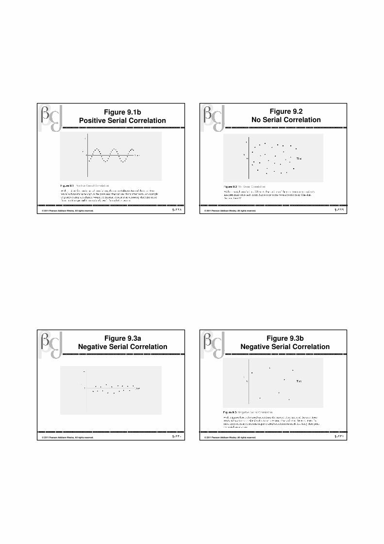
1-٢٢٨© 2011 Pearson Addison-Wesley. All rights reserved.

Figure 9.1b Positive Serial Correlation

1-٢٢٩© 2011 Pearson Addison-Wesley. All rights reserved.

Figure 9.2 No Serial Correlation

1-٢٣٠© 2011 Pearson Addison-Wesley. All rights reserved.

Figure 9.3a Negative Serial Correlation

1-٢٣١© 2011 Pearson Addison-Wesley. All rights reserved.

Figure 9.3b Negative Serial Correlation

1-٢٣٢© 2011 Pearson Addison-Wesley. All rights reserved.

Impure Serial Correlation

• Impure serial correlation is serial correlation that is caused by a specification error such as:

– an omitted variable and/or

– an incorrect functional form

• How does this happen?

• As an example, suppose that the true equation is:

(9.3)

where εt is a classical error term. As shown in Section 6.1, if X2 is accidentally omitted from the equation (or if data for X2 are unavailable), then:

(9.4)

• The error term is therefore not a classical error term

1-٢٣٣© 2011 Pearson Addison-Wesley. All rights reserved.

Impure Serial Correlation (cont.)

• Instead, the error term is also a function of one of the explanatory variables, X2

• As a result, the new error term, ε* , can be serially correlated even if the true error term ε, is not

• In particular, the new error term will tend to be serially correlated when:

1. X2 itself is serially correlated (this is quite likely in a time series) and

2. the size of ε is small compared to the size of

• Figure 9.4 illustrates 1., for the case of U.S. disposable income

1-٢٣٤© 2011 Pearson Addison-Wesley. All rights reserved.

Figure 9.4 U.S. Disposable Income as a Function of Time

1-٢٣٥© 2011 Pearson Addison-Wesley. All rights reserved.

Impure Serial Correlation (cont.)

• Turn now to the case of impure serial correlation caused by an incorrect functional form

• Suppose that the true equation is polynomial in nature:

(9.7)

but that instead a linear regression is run:

(9. 8)

• The new error term ε* is now a function of the true error term and of the differences between the linear and the polynomial functional

forms

• Figure 9.5 illustrates how these differences often follow fairlyautoregressive patterns

1-٢٣٦© 2011 Pearson Addison-Wesley. All rights reserved.

Figure 9.5a Incorrect Functional Form as a Source of Impure Serial Correlation

1-٢٣٧© 2011 Pearson Addison-Wesley. All rights reserved.

Figure 9.5b Incorrect Functional Form as a Source of Impure Serial Correlation

1-٢٣٨© 2011 Pearson Addison-Wesley. All rights reserved.

The Consequences of Serial Correlation

• The existence of serial correlation in the error term of an equation violates Classical Assumption IV, and the estimation of the equation with OLS has at least three consequences:

1. Pure serial correlation does not cause bias in the coefficient estimates

2. Serial correlation causes OLS to no longer be the minimum variance estimator (of all the linear unbiased estimators)

3. Serial correlation causes the OLS estimates of the SE to be biased, leading to unreliable hypothesis testing. Typically the bias in the SE estimate is negative, meaning that OLS underestimates the standard errors of the coefficients (and thus overestimates the t-scores)

1-٢٣٩© 2011 Pearson Addison-Wesley. All rights reserved.

The Durbin–Watson d Test

• Two main ways to detect serial correlation:

– Informal: observing a pattern in the residuals like that in Figure 9.1

– Formal: testing for serial correlation using the Durbin–Watson d test

• We will now go through the second of these in detail

• First, it is important to note that the Durbin–Watson d test is only applicable if the following three assumptions are met:

1. The regression model includes an intercept term

2. The serial correlation is first-order in nature: εt = ρεt–1 + ut

where ρ is the autocorrelation coefficient and u is a classical (normally distributed) error term

3. The regression model does not include a lagged dependent variable(discussed in Chapter 12) as an independent variable

1-٢٤٠© 2011 Pearson Addison-Wesley. All rights reserved.

• The equation for the Durbin–Watson d statistic for T observations is:

(9.10)

where the ets are the OLS residuals

• There are three main cases:

1. Extreme positive serial correlation: d = 0

2. Extreme negative serial correlation: d ≈ 4

3. No serial correlation: d ≈ 2

The Durbin–Watson d Test (cont.)

1-٢٤١© 2011 Pearson Addison-Wesley. All rights reserved.

• To test for positive (note that we rarely, if ever, test for negative!) serial correlation, the following steps are required:

1. Obtain the OLS residuals from the equation to be tested and calculate the d statistic by using Equation 9.10

2. Determine the sample size and the number of explanatory variables and then consult Statistical Tables B-4, B-5, or B-6 in Appendix B to find the upper critical d value, dU, and the lower critical d value, dL, respectively (instructions for the use of these tables are also in that appendix)


1-٢٤٢© 2011 Pearson Addison-Wesley. All rights reserved.


3. Set up the test hypotheses and decision rule:

H0: ρ ≤ 0 (no positive serial correlation)

HA: ρ > 0 (positive serial correlation)�if d < dL Reject H0

if d > dU Do not reject H0

if dL ≤ d ≤ dU Inconclusive

• In rare circumstances, perhaps first differenced equations, a two-sided d test might be appropriate

• In such a case, steps 1 and 2 are still used, but step 3 is now:

1-٢٤٣© 2011 Pearson Addison-Wesley. All rights reserved.

3. Set up the test hypotheses and decision rule:

H0: ρ = 0 (no serial correlation)

HA: ρ≠ 0 (serial correlation)

if d < dL Reject H0

if d > 4 – dL Reject H0

if 4 – dU > d > dU Do Not Reject H0

Otherwise Inconclusive

Figure 9.6 gives an example of a one-sided Durbin Watson dtest


1-٢٤٤© 2011 Pearson Addison-Wesley. All rights reserved.

Figure 9.6 An Example of a One-Sided Durbin–Watson d Test

1-٢٤٥© 2011 Pearson Addison-Wesley. All rights reserved.

Remedies for Serial Correlation

• The place to start in correcting a serial correlation problem is to look carefully at the specification of the equation for possible errors that might be causing impure serial correlation:

– Is the functional form correct?

– Are you sure that there are no omitted variables?

– Only after the specification of the equation has bee reviewed carefully should the possibility of an adjustment for pure serial correlation be considered

• There are two main remedies for pure serial correlation:

1. Generalized Least Squares

2. Newey-West standard errors

• We will no discuss each of these in turn

1-٢٤٦© 2011 Pearson Addison-Wesley. All rights reserved.

Generalized Least Squares

• Start with an equation that has first-order serial correlation:

(9.15)

• Which, if εt = ρεt–1 + ut (due to pure serial correlation), also equals:

(9.16)

• Multiply Equation 9.15 by ρ and then lag the new equation by one period, obtaining:

(9.17)

1-٢٤٧© 2011 Pearson Addison-Wesley. All rights reserved.

Generalized Least Squares (cont.)

• Next, subtract Equation 9.107 from Equation 9.16, obtaining:

(9.18)

• Finally, rewrite equation 9.18 as:

(9.19)

(9.20)

1-٢٤٨© 2011 Pearson Addison-Wesley. All rights reserved.


• Equation 9.19 is called a Generalized Least Squares(or “quasi-differenced”) version of Equation 9.16.

• Notice that:

1.The error term is not serially correlateda. As a result, OLS estimation of Equation 9.19 will be

minimum variance

b. This is true if we know ρ or if we accurately estimateρ)

2.The slope coefficientβ1 is the same as the slope coefficient of the original serially correlated equation, Equation 9.16. Thus coefficients estimated with GLS have the same meaning as those estimated with OLS.

1-٢٤٩© 2011 Pearson Addison-Wesley. All rights reserved.


3. The dependent variable has changed compared to that in Equation 9.16. This means that the GLS is not directly comparable to the OLS.

4. To forecast with GLS, adjustments like those discussed in Section 15.2 are required

• Unfortunately, we cannot use OLS to estimate a GLS model because GLS equations are inherently nonlinearin the coefficients

• Fortunately, there are at least two other methodsavailable:

1-٢٥٠© 2011 Pearson Addison-Wesley. All rights reserved.

The Cochrane–Orcutt Method

• Perhaps the best known GLS method

• This is a two-step iterative technique that first produces an estimate of ρ and then estimates the GLS equation using that estimate.

• The two steps are:1. Estimate ρ by running a regression based on the residuals of the equation

suspected of having serial correlation:

et = ρet–1 + ut (9.21)

where the ets are the OLS residuals from the equation suspected of having pure serial correlation and ut is a classical error term

2. Use this to estimate the GLS equation by substituting into Equation 9.18 and using OLS to estimate Equation 9.18 with the adjusted data

• These two steps are repeated (iterated) until further iteration results in little change in

• Once has converged (usually in just a few iterations), the last estimate of step 2 is used as a final estimate of Equation 9.18

1-٢٥١© 2011 Pearson Addison-Wesley. All rights reserved.

The AR(1) Method

• Perhaps a better alternative than Cochrane–Orcutt for GLS models

• The AR(1) method estimates a GLS equation like Equation 9.18 by estimating β0, β1 and ρ simultaneously with iterative nonlinear regression techniques (that are well beyond the scope of this chapter!)

• The AR(1) method tends to produce the same coefficient estimates as Cochrane–Orcutt

• However, the estimated standard errors are smaller

• This is why the AR(1) approach is recommended as long as your software can support such nonlinear regression

1-٢٥٢© 2011 Pearson Addison-Wesley. All rights reserved.

Newey–West Standard Errors

• Again, not all corrections for pure serial correlation involve Generalized Least Squares

• Newey–West standard errors take account of serial correlation by correcting the standard errors without changing the estimated coefficients

• The logic begin Newey–West standard errors is powerful:

– If serial correlation does not cause bias in the estimated coefficients but does impact the standard errors, then it makes sense to adjust the estimated equation in a way that changes the standard errors but not the coefficients

1-٢٥٣© 2011 Pearson Addison-Wesley. All rights reserved.

Newey–West Standard Errors (cont.)

• The Newey–West SEs are biased but generally more accurate than uncorrected standard errors for large samples in the face of serial correlation

• As a result, Newey–West standard errors can be used for t-tests and other hypothesis tests in most samples without the errors of inference potentially caused by serial correlation

• Typically, Newey–West SEs are larger than OLS SEs, thus producing lower t-scores

1-٢٥٤© 2011 Pearson Addison-Wesley. All rights reserved.


• Impure serial correlation

• First-order serial correlation

• First-order autocorrelation coefficient

• Durbin–Watson d statistic

• Generalized Least Squares (GLS)

• Positive serial correlation

• Newey–West standard errors

1-٢٥٥© 2011 Pearson Addison-Wesley. All rights reserved.

Chapter 10

Heteroskedasticity

1-٢٥٦© 2011 Pearson Addison-Wesley. All rights reserved. 10-٢٥٦© 2011 Pearson Addison-Wesley. All rights reserved.

Pure Heteroskedasticity

• Pure heteroskedasticity occurs when Classical Assumption V, which assumes constant variance of the error term, is violated (in a correctly specified equation!)

• Classical Assumption V assumes that:

(10.1)

• With heteroskedasticity, this error term variance is not constant

1-٢٥٧© 2011 Pearson Addison-Wesley. All rights reserved. 10-٢٥٧© 2011 Pearson Addison-Wesley. All rights reserved.

Pure Heteroskedasticity (cont.)

• Instead, the variance of the distribution of the error term depends on exactly which observation is being discussed:

(10.2)

• The simplest case is that of discrete heteroskedasticity, where the observations of the error term can be grouped into just two different distributions, “wide” and “narrow”

• This case is illustrated in Figure 10.1

1-٢٥٨© 2011 Pearson Addison-Wesley. All rights reserved. 10-٢٥٨© 2011 Pearson Addison-Wesley. All rights reserved.

Figure 10.1a Homoskedasticity versus Discrete Heteroskedasticity

1-٢٥٩© 2011 Pearson Addison-Wesley. All rights reserved. 10-٢٥٩© 2011 Pearson Addison-Wesley. All rights reserved.

Figure 10.1b Homoskedasticity versus Discrete Heteroskedasticity

1-٢٦٠© 2011 Pearson Addison-Wesley. All rights reserved. 10-٢٦٠© 2011 Pearson Addison-Wesley. All rights reserved.

Pure Heteroskedasticity (cont.)

• Heteroskedasticity takes on many more complex forms, however, than the discrete heteroskedasticity case

• Perhaps the most frequently specified model of pure heteroskedasticity relates the variance of the error term to an exogenous variable Zi as follows:

(10.3)

(10.4)

where Z, the “proportionality factor,” may or may not be in the equation

• This is illustrated in Figures 10.2 and 10.3

1-٢٦١© 2011 Pearson Addison-Wesley. All rights reserved. 10-٢٦١© 2011 Pearson Addison-Wesley. All rights reserved.

Figure 10.2 A Homoskedastic Error Term with Respect to Zi

1-٢٦٢© 2011 Pearson Addison-Wesley. All rights reserved. 10-٢٦٢© 2011 Pearson Addison-Wesley. All rights reserved.

Figure 10.3 A Heteroskedastic Error Term with Respect to Zi

1-٢٦٣© 2011 Pearson Addison-Wesley. All rights reserved. 10-٢٦٣© 2011 Pearson Addison-Wesley. All rights reserved.

Impure Heteroskedasticity

• Similar to impure serial correlation, impure heteroskedasticity is heteroskedasticity that is caused by a specification error

• Contrary to that case, however, impure heteroskedasticity almost always originates from an omitted variable (rather than an incorrect functional form)


– The portion of the omitted effect not represented by one of the included explanatory variables must be absorbed by the error term.

– So, if this effect has a heteroskedastic component, the error term of the

misspecified equation might be heteroskedastic even if the error term of the true equation is not!

• This highlights, again, the importance of first checking that the specification is correct before trying to “fix” things…

1-٢٦٤© 2011 Pearson Addison-Wesley. All rights reserved. 10-٢٦٤© 2011 Pearson Addison-Wesley. All rights reserved.

The Consequences of Heteroskedasticity

• The existence of heteroskedasticity in the error term of an equation violates Classical Assumption V, and the estimation of the equation with OLS has at least three consequences:

1. Pure heteroskedasticity does not cause bias in the coefficient estimates

2. Heteroskedasticity typically causes OLS to no longer be the minimum variance estimator (of all the linear unbiased

estimators)

3. Heteroskedasticity causes the OLS estimates of the SE to be biased, leading to unreliable hypothesis testing. Typically the bias in the SE estimate is negative, meaning that OLS

underestimates the standard errors (and thus overestimates the t-scores)

1-٢٦٥© 2011 Pearson Addison-Wesley. All rights reserved. 10-٢٦٥© 2011 Pearson Addison-Wesley. All rights reserved.

Testing for Heteroskedasticity

• Econometricians do not all use the same test for heteroskedasticity because heteroskedasticity takes a number of different forms, and its precise manifestation in a given equation is almost never known

• Before using any test for heteroskedasticity, however, ask the following:

1. Are there any obvious specification errors? – Fix those before testing!

2. Is the subject of the research likely to be afflicted with heteroskedasticity? – Not only are cross-sectional studies the most frequent source of

heteroskedasticity, but cross-sectional studies with large variations in the size of the dependent variable are particularly susceptible to heteroskedasticity

3. Does a graph of the residuals show any evidence of heteroskedasticity? – Specifically, plot the residuals against a potential Z proportionality factor

– In such cases, the graph alone can often show that heteroskedasticity is or is not likely

– Figure 10.4 shows an example of what to look for: an expanding (or contracting) range of the residuals

1-٢٦٦© 2011 Pearson Addison-Wesley. All rights reserved. 10-٢٦٦© 2011 Pearson Addison-Wesley. All rights reserved.

Figure 10.4 Eyeballing Residuals for Possible Heteroskedasticity

1-٢٦٧© 2011 Pearson Addison-Wesley. All rights reserved. 10-٢٦٧© 2011 Pearson Addison-Wesley. All rights reserved.

The Park Test

The Park test has three basic steps:

1. Obtain the residuals of the estimated regression equation:

(10.6)

2. Use these residuals to form the dependent variable in a second regression:

(10.7)

where: ei = the residual from the ith observation from Equation 10.6

Zi = your best choice as to the possible proportionality factor (Z)ui = a classical (homoskedastic) error term

1-٢٦٨© 2011 Pearson Addison-Wesley. All rights reserved. 10-٢٦٨© 2011 Pearson Addison-Wesley. All rights reserved.

The Park Test

3. Test the significance of the coefficient of Z in Equation 10.7 with a t-test:

– If the coefficient of Z is statistically significantly different from

zero, this is evidence of heteroskedastic patterns in the residuals with respect to Z

– Potential issue: How do we choose Z in the first place?

1-٢٦٩© 2011 Pearson Addison-Wesley. All rights reserved. 10-٢٦٩© 2011 Pearson Addison-Wesley. All rights reserved.

The White Test

• The White test also has three basic steps:

1. Obtain the residuals of the estimated regression equation:

– This is identical to the first step in the Park test

2. Use these residuals (squared) as the dependent variable in a second equation that includes as explanatory variables each X from the original equation, the square of each X, and the product of each X times every other X—for example, in the case of three explanatory variables:

(10.9)

1-٢٧٠© 2011 Pearson Addison-Wesley. All rights reserved. 10-٢٧٠© 2011 Pearson Addison-Wesley. All rights reserved.

The White Test (cont.)

3. Test the overall significance of Equation 10.9 with the chi-square test

– The appropriate test statistic here is NR2, or the sample size (N) times the coefficient of determination (the unadjusted R2) of Equation 10.9

– This test statistic has a chi-square distribution with degrees of freedom equal to the number of slope coefficients in Equation 10.9

– If NR2 is larger than the critical chi-square value found in Statistical Table B-8, then we reject the null hypothesis and conclude that it's likely that we have heteroskedasticity

– If NR2 is less than the critical chi-square value, then we cannot reject the null hypothesis of homoskedasticity

1-٢٧١© 2011 Pearson Addison-Wesley. All rights reserved. 10-٢٧١© 2011 Pearson Addison-Wesley. All rights reserved.

Remedies for Heteroskedasticity

• The place to start in correcting a heteroskedasticity problem is to look carefully at the specification of the equation for possible errors that might be causing impure heteroskedasticity :

– Are you sure that there are no omitted variables?

– Only after the specification of the equation has been reviewed carefully should the possibility of an adjustment for pure heteroskedasticity be considered

• There are two main remedies for pure heteroskedasticit1

1. Heteroskedasticity-corrected standard errors

2. Redefining the variables

• We will now discuss each of these in turn:

1-٢٧٢© 2011 Pearson Addison-Wesley. All rights reserved. 10-٢٧٢© 2011 Pearson Addison-Wesley. All rights reserved.

Heteroskedasticity-Corrected Standard Errors

• Heteroskedasticity-corrected errors take account of heteroskedasticity correcting the standard errors without changing the estimated coefficients

• The logic behind heteroskedasticity-corrected standard errors is power

– If heteroskedasticity does not cause bias in the estimated coefficients but does impact the standard errors, then it makes sense to adjust the estimated equation in a way that changes the standard errors but not the coefficients

1-٢٧٣© 2011 Pearson Addison-Wesley. All rights reserved. 10-٢٧٣© 2011 Pearson Addison-Wesley. All rights reserved.

Heteroskedasticity-Corrected Standard Errors (cont.)

• The heteroskedasticity-corrected SEs are biased but generally more accurate than uncorrected standard errors for large samples in the face of heteroskedasticity

• As a result, heteroskedasticity-corrected standard errors can be used for t-tests and other hypothesis tests in most samples without the errors of inference potentially caused by heteroskedasticity

• Typically heteroskedasticity-corrected SEs are larger than OLS SEs, thus producing lower t-scores

1-٢٧٤© 2011 Pearson Addison-Wesley. All rights reserved. 10-٢٧٤© 2011 Pearson Addison-Wesley. All rights reserved.

Redefining the Variables

• Sometimes it’s possible to redefine the variables in a way that avoids heteroskedasticity

• Be careful, however:

– Redefining your variables is a functional form specification

change that can dramatically change your equation!

• In some cases, the only redefinition that's needed to rid an equation of heteroskedasticity is to switch from a linear functional form to a double-log functional form:

– The double-log form has inherently less variation than the linear form, so it's less likely to encounter heteroskedasticity

1-٢٧٥© 2011 Pearson Addison-Wesley. All rights reserved. 10-٢٧٥© 2011 Pearson Addison-Wesley. All rights reserved.

Redefining the Variables (cont.)

• In other situations, it might be necessary to completely rethink the research project in terms of its underlying theory

• For example, a cross-sectional model of the total expenditures by the governments of different cities may generate heteroskedasticity by containing both large and small cities in the estimation sample

• Why?

– Because of the proportionality factor (Z) the size of the cities

1-٢٧٦© 2011 Pearson Addison-Wesley. All rights reserved. 10-٢٧٦© 2011 Pearson Addison-Wesley. All rights reserved.

Redefining the Variables (cont.)

• This is illustrated in Figure 10.5

• In this case, per capita expenditures would be a logical dependent variable

• Such a transformation is shown in Figure 10.6

• Aside: Note that Weighted Least Squares (WLS), that some authors suggest as a remedy for heteroskedasticity, has some serious potential drawbacks and can therefore generally is not be recommended (see Footnote 14, p. 355, for details)

1-٢٧٧© 2011 Pearson Addison-Wesley. All rights reserved. 10-٢٧٧© 2011 Pearson Addison-Wesley. All rights reserved.

Figure 10.5 An Aggregate City Expenditures Function

1-٢٧٨© 2011 Pearson Addison-Wesley. All rights reserved. 10-٢٧٨© 2011 Pearson Addison-Wesley. All rights reserved.

Figure 10.6 A Per Capita City Expenditures Function

1-٢٧٩© 2011 Pearson Addison-Wesley. All rights reserved. 10-٢٧٩© 2011 Pearson Addison-Wesley. All rights reserved.

Table 10.1a

1-٢٨٠© 2011 Pearson Addison-Wesley. All rights reserved. 10-٢٨٠© 2011 Pearson Addison-Wesley. All rights reserved.

Table 10.1b

1-٢٨١© 2011 Pearson Addison-Wesley. All rights reserved. 10-٢٨١© 2011 Pearson Addison-Wesley. All rights reserved.

Table 10.1c

1-٢٨٢© 2011 Pearson Addison-Wesley. All rights reserved. 10-٢٨٢© 2011 Pearson Addison-Wesley. All rights reserved.


• Impure heteroskedasticity

• Pure heteroskedasticity

• Proportionality factor Z

• The Park test

• The White test

• Heteroskedasticity-corrected standard errors

1-٢٨٣© 2011 Pearson Addison-Wesley. All rights reserved.

Chapter 11

Running Your Own Regression Project

1-٢٨٤© 2011 Pearson Addison-Wesley. All rights reserved.

Choosing Your Topic

• There are at least three keys to choosing a topic:

1. Try to pick a field that you find interesting and/or that you know something about

2. Make sure that data are readily available with a reasonable sample (we suggest at least 25 observations)

3. Make sure that there is some substance to your topic

– Avoid topics that are purely descriptive or virtually tautological in nature

– Instead, look for topics that address an inherently interesting economic or behavioral question or choice

1-٢٨٥© 2011 Pearson Addison-Wesley. All rights reserved.

Choosing Your Topic (cont.)

• Places to look:

– your textbooks and notes from previous economics classes

– economics journals

• For example, Table 11.1 contains a list of the journals cited so far in this textbook (in order of the frequency of citation)

1-٢٨٦© 2011 Pearson Addison-Wesley. All rights reserved.

Table 11.1a

Sources of Potential Topic Ideas

1-٢٨٧© 2011 Pearson Addison-Wesley. All rights reserved.

Table 11.1b

Sources of Potential Topic Ideas

1-٢٨٨© 2011 Pearson Addison-Wesley. All rights reserved.

Collecting Your Data

• Before any quantitative analysis can be done, the data must be:

– collected

– organized

– entered into a computer

• Usually, this is a time-consuming and frustrating task because of:

– the difficulty of finding data

– the existence of definitional differences between theoretical variables and their empirical counterparts

– and the high probability of data entry errors or data transmission errors

• But time spent thinking about and collecting the data is well spent, since a researcher who knows the data sources and definitions is much less likely to make mistakes using or interpreting regressions run on that data

• We will now discuss three data collection issues in a bit more detail 1-٢٨٩© 2011 Pearson Addison-Wesley. All rights reserved.

What Data to Look For

• Checking for data availability means deciding what specific variables you want to study:

– dependent variable

– all relevant independent variables

• At least 5 issues to consider here:

1. Time periods:

– If the dependent variable is measured annually, the explanatory variables should also be measured annually and not, say, monthly

2. Measuring quantity:

– If the market and/or quality of a given variable has changed over time, it makes little sense to use quantity in units

– Example: TVs have changed so much over time that it makes more sense to use quantity in terms of monetary equivalent: more comparable across time

1-٢٩٠© 2011 Pearson Addison-Wesley. All rights reserved.

What Data to Look For (cont.)

3. Nominal or real terms?

– Depends on theory – essentially: do we want to “clean” for inflation?

– TVs, again: probably use real terms

4. Appropriate variable definitions depend on whether data are cross-sectional or time-series

– TVs, again: national advertising would be a good candidate for an explanatory variable in a time-series model, while advertising in or near

each state (or city) would make sense in a cross-sectional model

5. Be careful when reading (and creating!) descriptions of data:

– Where did the data originate?

– Are prices and/or income measured in nominal or real terms?

– Are prices retail or wholesale?1-٢٩١© 2011 Pearson Addison-Wesley. All rights reserved.

Where to Look forEconomic Data

• Although some researchers generate their own data through surveys or other techniques (see Section 11.3), the vast majority of regressions are run on publicly available data

• Good sources here include:

1. Government publications:

– Statistical Abstract of the U.S.

– the annual Economic Report of the President

– the Handbook of Labor Statistics

– Historical Statistics of the U.S. (published in 1975)

– Census Catalog and Guide

1-٢٩٢© 2011 Pearson Addison-Wesley. All rights reserved.

Where to Look for Economic Data (cont.)

2. International data sources:

– U.N. Statistical Yearbook

– U.N. Yearbook of National Account Statistics

3. Internet resources:

– “Resources for Economists on the Internet”

– Economagic

– WebEC

– EconLit (www.econlit.org)

– “Dialog”

– Links to these sites and other good sources of data are on the text’s Web site: www.pearsonhighered.com/studenmund 1-٢٩٣© 2011 Pearson Addison-Wesley. All rights reserved.

Missing Data

• Suppose the data aren’t there?– What happens if you choose the perfect variable and

look in all the right sources and can’t find the data?– The answer to this question depends on how much

data is missing:

1. A few observations:– in a cross-section study:

• Can usually afford to drop these observations from the sample

– in a time-series study:• May interpolate value (taking the mean of adjacent values)

1-٢٩٤© 2011 Pearson Addison-Wesley. All rights reserved.

Missing Data (cont.)

2. No data at all available (for a theoretically relevant variable!):– From Chapter 6, we know that this is likely to cause

omitted variables bias

– A possible solution here is to use a proxy variable

– For example, the value of net investment is a variable that is not measured directly in a number of countries

– Instead, might use the value of gross investment as a proxy, the assumption being that the value of gross investment is directly proportional to the value of net investment

1-٢٩٥© 2011 Pearson Addison-Wesley. All rights reserved.

Advanced Data Sources

• So far, all the data sets have been:1. cross-sectional or time-series in nature

2. been collected by observing the world around us, instead being created

• It turns out, however, that:1. time-series and cross-sectional data can be pooled to form panel

data

2. data can be generated through surveys

• We will now briefly introduce these more advanced data sources and explain why it probably doesn't make sense to use these data sources on your first regression project:

1-٢٩٦© 2011 Pearson Addison-Wesley. All rights reserved.

Surveys

• Surveys are everywhere in our society and are used for many different purposes—examples include:– marketing firms using surveys to learn more about

products and competition

– political candidates using surveys to finetune their campaign advertising or strategies

– governments using surveys for all sorts of purposes, including keeping track of their citizens with instruments like the U.S. Census

1-٢٩٧© 2011 Pearson Addison-Wesley. All rights reserved.

Surveys (cont.)

• While running your own survey might be tempting as a way of obtaining data for your own project, running a survey is not as easy as it might seem surveys:

– must be carefully thought through; it’s virtually impossible to go

– back to the respondents and add another question later

– must be worded precisely (and pretested) to avoid confusing the respondent or "leading" the respondent to a particular answer

– must have samples that are random and avoid the selection, survivor, and nonresponse biases explained in Section 17.2

• As a result, we don't encourage beginning researchers to run their own surveys...

1-٢٩٨© 2011 Pearson Addison-Wesley. All rights reserved.

Panel Data

• Again, panel data are formed when cross-sectional and time-series data sets are pooled to create a single data set

• Two main reasons for using panel data:

– To increase the sample size

– To provide an insight into an analytical question that can't be

obtained by using time-series or cross-sectional data alone

1-٢٩٩© 2011 Pearson Addison-Wesley. All rights reserved.

Panel Data (cont.)

• Example: suppose we’re interested in the relationship between budget deficits and interest rates but only have 10 years’ of annual data to study – But ten observations is too small a sample for a reasonable

regression!

– However, if we can find time-series data on the same economic variables-interest rates and budget deficits—for the same ten years for six different countries, we’ll end up with a sample of 10*6 = 60 observations, which is more than enough

– The result is a pooled cross-section time-series data set—a panel data set!

– Panel data estimation methods are treated in Chapter 16

1-٣٠٠© 2011 Pearson Addison-Wesley. All rights reserved.

Practical Advice for Your Project

• We now move to a discussion of practical advice about actually doing applied econometric work

• This discussion is structured in three parts:

1. The 10 Commandments of Applied Econometrics (by Peter Kennedy)

2. What to check if you get an unexpected sign

3. A collection of a dozen practical tips, brought together from other sections of this text that are worth reiterating specifically in the context of actually doing applied econometric work

1-٣٠١© 2011 Pearson Addison-Wesley. All rights reserved.

Practical Advice for Your Project

• We now move to a discussion of practical advice about actually doing applied econometric work

• This discussion is structured in three parts:

1. The 10 Commandments of Applied Econometrics (by Peter Kennedy)

2. What to check if you get an unexpected sign

3. A collection of a dozen practical tips, brought together from other sections of this text that are worth reiterating specifically in the context of actually doing applied econometric work

1-٣٠٢© 2011 Pearson Addison-Wesley. All rights reserved.

The 10 Commandments of Applied Econometrics

1. Use common sense and economic theory:

Example: match per capita variables with per capita variables, use real exchange rates to explain real imports or exports, etc

2. Ask the right questions:

Ask plenty of, perhaps, seemingly silly questions to ensure that you fully understand the goal of the research

3. Know the context:

Be sure to be familiar with the history, institutions, operating constraints, measurement peculiarities, cultural customs, etc, underlying the object under study

4. Inspect the data:

a. This includes calculating summary statistics, graphs, and data cleaning (including checking filters)

b. The objective is to get to know the data well

1-٣٠٣© 2011 Pearson Addison-Wesley. All rights reserved.

5. Keep it sensibly simple:

a. Begin with a simple model and only complicate it if it fails

b. This both goes for the specifications, functional forms, etc and for the estimation method

6. Look long and hard at your results:

a. Check that the results make sense, including signs and magnitudes

b. Apply the “laugh test”

7. Understand the costs and benefits of data mining:

a. “Bad” data mining: deliberately searching for a specification that “works”(i.e. “torturing” the data)

b. “Good” data mining: experimenting with the data to discover empirical regularities that can inform economic theory and be tested on a second data set

The 10 Commandments of Applied Econometrics (cont.)

1-٣٠٤© 2011 Pearson Addison-Wesley. All rights reserved.


8. Be prepared to compromise:

a. The Classical Assumptions are only rarely are satisfied

b. Applied econometricians are therefore forced to compromise and adopt suboptimal solutions, the characteristics and consequences of which are not always known

c. Applied econometrics is necessarily ad hoc: we develop our analysis, including responses to potential problems, as we go along…

9. Do not confuse statistical significance with meaningful magnitude:

a. If the sample size is large enough, any (two-sided) hypothesis can be rejected (when large enough to make the SEs small enough)

b. Substantive significance—i.e. “how large?”—is also important, not just statistical significance

1-٣٠٥© 2011 Pearson Addison-Wesley. All rights reserved.


10. Report a sensitivity analysis:

a. Dimensions to examine:

i. sample period

ii. the functional form

iii. the set of explanatory variables

iv. the choice of proxies

b. If results are not robust across the examined dimensions, then this casts doubt on the conclusions of the research

1-٣٠٦© 2011 Pearson Addison-Wesley. All rights reserved.

What to Check If You Get an Unexpected Sign

1. Recheck the expected sign

Were dummy variables computed “upside down,” for example?

2. Check your data for input errors and/or outliers

3. Check for an omitted variable

The most frequent source of significant unexpected signs

4. Check for an irrelevant variable

Frequent source of insignificant unexpected signs

5. Check for multicollinearity

Multicollinearity increases the variances and standard errors of the estimated coefficients, increasing the chance that a coefficient could have an unexpected sign

1-٣٠٧© 2011 Pearson Addison-Wesley. All rights reserved.

6. Check for sample selection bias

An unexpected sign sometimes can be due to the fact that the

observations included in the data were not obtained randomly

7. Check your sample size

The smaller the sample size, the higher the variance on SEs

8. Check your theory

If nothing else is apparently wrong, only two possibilities remain: the theory is wrong or the data is bad

What to Check If You Get an Unexpected Sign

1-٣٠٨© 2011 Pearson Addison-Wesley. All rights reserved.

A Dozen Practical Tips Worth Reiterating

1. Don’t attempt to maximize (Chapter 2)

2. Always review the literature and hypothesize the signsof your coefficients before estimating a model (Chapter 3)

3. Inspect and clean your data before estimating a model. Know that outliers should not be automatically omitted; instead, they should be investigated to make sure that they belong in the sample (Chapter 3)

4. Know the Classical Assumptions cold! (Chapter 4)

5. In general, use a one-sided t-test unless the expected sign of the coefficient actually is in doubt (Chapter 5)

R2

1-٣٠٩© 2011 Pearson Addison-Wesley. All rights reserved.

6. Don’t automatically discard a variable with an insignificant t-score. In general, be willing to live with a variable with a t-score lower than the critical value in order to decrease the chance of omitting a relevant variable (Chapter 6)

7. Know how to analyze the size and direction of the biascaused by an omitted variable (Chapter 6)

8. Understand all the different functional form options and their common uses, and remember to choose your functional form primarily on the basis of theory, not fit(Chapter 7)

A Dozen Practical Tips Worth Reiterating (cont.)

1-٣١٠© 2011 Pearson Addison-Wesley. All rights reserved.

9. Multicollinearity doesn’t create bias; the estimated variances are large, but the estimated coefficients themselves are unbiased: So, the most-used remedy for multicollinearity is to do nothing (Chapter 8)

10. If you get a significant Durbin–Watson, Park, or White test, remember to consider the possibility that a specification error might be causing impure serial correlation or heteroskedasticity. Don’t change your estimation technique from OLS to GLS or use adjusted standard errors until you have the best possible specification. (Chapters 9 and 10)


1-٣١١© 2011 Pearson Addison-Wesley. All rights reserved.

11. Adjusted standard errors like Newey–West standard errors or HC standard errors use the OLS coefficient estimates. It’s the standard errors of the estimated coefficients that change, not the estimated coefficients themselves. (Chapters 9 and 10)

12. Finally, if in doubt, rely on common sense and economic theory, not on statistical tests


1-٣١٢© 2011 Pearson Addison-Wesley. All rights reserved.

The Ethical Econometrician

• We think that there are two reasonable goals for econometricians when estimating models:1. Run as few different specifications as possible while

still attempting to avoid the major econometric problems• The only exception is sensitivity analysis, described in

Section 6.4

2. Report honestly the number and type of different specifications estimated so that readers of the research can evaluate how much weight to give to your results

1-٣١٣© 2011 Pearson Addison-Wesley. All rights reserved.

Writing Your Research Report

• Most good research reports have a number of elements in common:– A brief introduction that defines the dependent variable and states

the goals of the research

– A short review of relevant previous literature and research

– An explanation of the specification of the equation (model):

• Independent variables

• functional forms

• expected signs of (or other hypotheses about) the slope coefficients

– A description of the data:

• generated variables

• data sources

• data irregularities (if any)

1-٣١٤© 2011 Pearson Addison-Wesley. All rights reserved.

Writing Your Research Report (cont.)

• A presentation of each estimated specification, using our standard documentation format– If you estimate more than one specification, be sure to explain which one is

best (and why!)

• A careful analysis of the regression results:

– discussion of any econometric problems encountered

– complete documentation of all:

• equations estimated

• tests run

• A short summary/conclusion that includes any policy recommendations or suggestions for further research

• A bibliography

• An appendix that includes all data, all regression runs, and all relevant computer output

1-٣١٥© 2011 Pearson Addison-Wesley. All rights reserved.

Table 11.2a Regression User’s Checklist

1-٣١٦© 2011 Pearson Addison-Wesley. All rights reserved.

Table 11.2b Regression User’s Checklist

1-٣١٧© 2011 Pearson Addison-Wesley. All rights reserved.

Table 11.2c Regression User’s Checklist

1-٣١٨© 2011 Pearson Addison-Wesley. All rights reserved.

Table 11.2d Regression User’s Checklist

1-٣١٩© 2011 Pearson Addison-Wesley. All rights reserved.

Table 11.3a Regression User’s Guide

1-٣٢٠© 2011 Pearson Addison-Wesley. All rights reserved.

Table 11.3b Regression User’s Guide

1-٣٢١© 2011 Pearson Addison-Wesley. All rights reserved.

Table 11.3c Regression User’s Guide

1-٣٢٢© 2011 Pearson Addison-Wesley. All rights reserved.


• Choosing a research topic

• Data collection

• Missing data

• Surveys

• Panel data

• The 10 Commandments of Applied Econometrics

• What to Check If You Get An Unexpected Sign

• A Dozen Practical Tips Worth Reiterating

• The Ethical Econometrician

• Writing your research report

• A Regression User’s Checklist

• A Regression User’s Guide

1-٣٢٣© 2011 Pearson Addison-Wesley. All rights reserved.

Chapter 12

Time-Series Models

1-٣٢٤© 2011 Pearson Addison-Wesley. All rights reserved.

Dynamic Models: Distributed Lag Models

• An (ad hoc) distributed lag model explains the current value of Y as a function of current and past values of X, thus “distributing” the impact of X over a number of time periods

• For example, we might be interested in the impact of a change in the money supply (X) on GDP (Y) and model this as:

Yt = α0 + β0Xt + β1Xt–1 + β2Xt–2 + ... + βpXt–p + εt (12.2)

• Potential issues from estimating Equation 12.2 with OLS:

1. The various lagged values of X are likely to be severely multicollinear, making coefficient estimates imprecise

1-٣٢٥© 2011 Pearson Addison-Wesley. All rights reserved.

Dynamic Models: Distributed Lag Models (cont.)

2. In large part because of this multicollinearity, there is no guarantee that the estimated coefficients will follow the smoothly declining pattern that economic theory would suggest

Instead, it’s quite typical to get something like:

3. The degrees of freedom tend to decrease, sometimes substantially, since we have to:

a. estimate a coefficient for each lagged X, thus increasing K and lowering

the degrees of freedom (N – K – 1)

b. decrease the sample size by one for each lagged X, thus lowering the

number of observations, N, and therefore the degrees of freedom (unless data for lagged Xs outside the sample are available)

1-٣٢٦© 2011 Pearson Addison-Wesley. All rights reserved.

What Is a Dynamic Model?

• The simplest dynamic model is:

(12.3)

• Note that Y is on the left-hand side as Yt, and on the right-hand side as Yt–1

– It’s this difference in time period that makes the equation dynamic

• Note that there is an important connection between a dynamic model such as the Equation 12.3 and a distributed lag model such as Equation 12.2

Yt= α

0+ β

0X

t+ λY

t−1+ u

t

1-٣٢٧© 2011 Pearson Addison-Wesley. All rights reserved.

What Is a Dynamic Model? (cont.)

Yt = α0 + β0Xt + β1Xt–1 + β2Xt–2 + ... + βpXt–p + εt

(12.2)

where: β1 = λβ0 (12.8)β2 = λ2β0β3 = λ3β0

.

.βp = λPβ0

• As long as λ is between 0 and 1, these coefficients will indeed smoothly decline, as shown in Figure 12.1

1-٣٢٨© 2011 Pearson Addison-Wesley. All rights reserved.

Figure 12.1 Geometric Weighting Schemes for Various Dynamic Models

1-٣٢٩© 2011 Pearson Addison-Wesley. All rights reserved.

Serial Correlation and Dynamic Models

• The consequences of serial correlation depend crucially on the type of model in question:

1. Ad hoc distributed lag models:

– serial correlation has the effects outlined in Section 9.2:

• causes no bias in the OLS coefficients themselves

• causes OLS to no longer be the minimum variance unbiased estimator

• causes the standard errors to be biased

2. Dynamic models:

– Now serial correlation causes bias in the coefficients produced by OLS

• Compounding all this this is the fact that the consequences, detection, and remedies for serial correlation that we discussed in Chapter 9 are all either incorrect or need to be modified in the presence of a lagged dependent variable

• We will now discuss the issues of testing and correcting for serial correlationin dynamic models in a bit more detail

1-٣٣٠© 2011 Pearson Addison-Wesley. All rights reserved.

Testing for Serial Correlation in Dynamic Models

• Using the Lagrange Multiplier to test for serial correlation for a typical dynamic model involves three steps:

1. Obtain the residuals of the estimated equation:

2. Use these residuals as the dependent variable in an auxiliary

regression that includes as independent variables all those on the right-hand side of the original equation as well as the lagged residuals:

et= Y

t− öY

t= Y

t− öα

0− öβ

0X

1t− λY

t−1

1-٣٣١© 2011 Pearson Addison-Wesley. All rights reserved.

Testing for Serial Correlation in Dynamic Models (cont.)

3. Estimate Equation 12.18 using OLS and then test the null hypothesis that a3 = 0 with the following test statistic:

LM = N*R2 (12.19)

where: N = the sample size R2 is the unadjusted coefficient of determination

both of the auxiliary equation, Equation 12.18

For large samples, LM has a chi-square distribution with degrees of freedom equal to the number of restrictions in the null hypothesis (in this case, one).

If LM is greater than the critical chi-square value from Statistical Table B-8, then we reject the null hypothesis that a3 = 0 and conclude that there is indeed serial correlation in the original equation

1-٣٣٢© 2011 Pearson Addison-Wesley. All rights reserved.

Correcting for Serial Correlation in Dynamic Models

• There are essentially three strategies for attempting to rid a dynamic model of serial correlation:

• improving the specification:

– Only relevant if the serial correlation is impure

• instrumental variables:

– substituting an “instrument” (a variable that is highly correlated with YM but is uncorrelated with ut) for Yt: in the original equation effectively eliminates the correlation between Ytl and ut

– Problem: good instruments are hard to come by (also see Section 14.3)

• modified GLS:

– Technique similar to the GLS procedure outlined in Section 9.4

– Potential issues: sample must be large and the standard

1-٣٣٣© 2011 Pearson Addison-Wesley. All rights reserved.

Granger Causality

• Granger causality, or precedence, is a circumstance in which one time series variable consistently and predictably changes before another variable

• A word of caution: even if one variable precedes (“Granger causes”) another, this does not mean that the first variable “causes” the other to change

• There are several tests for Granger causality

• They all involve distributed lag models in one form or another, however

• We’ll discuss an expanded version of a test originally developed by Granger

1-٣٣٤© 2011 Pearson Addison-Wesley. All rights reserved.

Granger Causality (cont.)

• Granger suggested that to see if A Granger-caused Y, we should run:

Yt = β0 + β1Yt–1 + ... + βpYt–p + α1At–1 + ... + αpAt–p + εt

(12.20)

and test the null hypothesis that the coefficients of the lagged As (the αs) jointly equal zero

• If we can reject this null hypothesis using the F-test, then we have evidence that A Granger-causes Y

• Note that if p = 1, Equation 12.20 is similar to the dynamic

model, Equation 12.3

• Applications of this test involve running two Granger tests, one in each direction

1-٣٣٥© 2011 Pearson Addison-Wesley. All rights reserved.

• That is, run Equation 12.20 and also run:

At = β0 + β1At–1 + ... + βpAt–p + α1Yt–1 + ... + αpYt–p + εt

(12.21)

testing for Granger causality in both directions by testing the null hypothesis that the coefficients of the lagged Ys (again, the αs) jointly equal zero

• If the F-test is significant for Equation 12.20 but notfor Equation 12.21, then we can conclude that A Granger-causes Y

Granger Causality (cont.)

1-٣٣٦© 2011 Pearson Addison-Wesley. All rights reserved.

Spurious Correlation and Nonstationarity

• Independent variables can appear to be more significant than they actually are if they have the same underlying trend as the dependent variable

• Example: In a country with rampant inflation almost any nominal variable will appear to be highly correlated with all other nominal variables

• Why?

– Nominal variables are unadjusted for inflation, so every nominal variable will have a powerful inflationary component

• Such a problem is an example of spurious correlation:

– a strong relationship between two or more variables that is not caused by a real underlying causal relationship

– If you run a regression in which the dependent variable and one or more independent variables are spuriously correlated, the result is a spurious regression, and the t-scores and overall fit of such spurious regressions are likely to be overstated and untrustworthy

1-٣٣٧© 2011 Pearson Addison-Wesley. All rights reserved.

Stationary and Nonstationary Time Series

• a time-series variable, Xt, is stationary if:

1. the mean of Xt is constant over time,

2. the variance of Xt is constant over time, and

3. the simple correlation coefficient between Xt and Xt–k depends on the length of the lag (k) but on no other variable (for all k)

• If one or more of these properties is not met, then Xt is nonstationary

• If a series is nonstationary, that problem is often referred to as nonstationarity

1-٣٣٨© 2011 Pearson Addison-Wesley. All rights reserved.

Stationary and Nonstationary Time Series (cont.)

• To get a better understanding of these issues, consider the case where Yt is generated by an equation that includes only past values of itself (an autoregressive equation):

Yt = γYt–1 + vt (12.22)

where vt is a classical error term

• Can you see that if | γ | < 1, then the expected value of Yt will eventually approach 0 (and therefore be stationary) as the sample size gets bigger and bigger? (Remember, since vt is a classical error term, its expected value = 0)

• Similarly, can you see that if | γ | > 1, then the expected value of Yt will continuously increase, making Yt nonstationary?

• This is nonstationarity due to a trend, but it still can cause spurious regression results

1-٣٣٩© 2011 Pearson Addison-Wesley. All rights reserved.

Stationary and Nonstationary Time Series (cont.)

• Most importantly, what about if |γ| = 1? In this case:

Yt = Yt–1 + vt (12.23)

• This is a random walk: the expected value of Yt does not converge on any value, meaning that it is nonstationary

• This circumstance, where γ = 1 in Equation 12.23 (or similar equations), is called a unit root

• If a variable has a unit root, then Equation 12.23 holds, and the variable follows a random walk and is nonstationary

1-٣٤٠© 2011 Pearson Addison-Wesley. All rights reserved.

The Dickey–Fuller Test

• From the previous discussion of stationarity and unit roots, it makes sense to estimate Equation 12.22:

Yt = γYt–1 + vt (12.22)

and then determine if |γ| < 1 to see if Y is stationary

• This is almost exactly how the Dickey-Fuller test works:

1. Subtract Yt–1 from both sides of Equation 12.22, yielding:

(Yt – Yt–1) = (γ – 1)Yt–1 + vt (12.26)

1-٣٤١© 2011 Pearson Addison-Wesley. All rights reserved.

The Dickey–Fuller Test (cont.)

If we define ΔYt = Yt – Yt–1 then we have the simplest form of the Dickey–Fuller test:ΔYt = β1Yt–1 + vt (12.27)

where β1 = γ – 1

• Note: alternative Dickey-Fuller tests additionally include a constant and/or a constant and a trend term

2. Set up the test hypotheses:

H0: β1 = 0 (unit root)

HA: β1 < 0 (stationary)

1-٣٤٢© 2011 Pearson Addison-Wesley. All rights reserved.

The Dickey–Fuller Test (cont.)

3. Set up the decision rule:

If is statistically significantly less than 0, then we can reject the null hypothesis of nonstationarity

If is not statistically significantly less than 0, then we cannot reject the null hypothesis of nonstationarity

• Note that the standard t-table does not apply to Dickey–Fuller tests

• For the case of no constant and no trend (Equation 12.27) the large-sample values for tc are listed in Table 12.1

1-٣٤٣© 2011 Pearson Addison-Wesley. All rights reserved.

Table 12.1 Large-Sample Critical Values for the Dickey–Fuller Test

1-٣٤٤© 2011 Pearson Addison-Wesley. All rights reserved.

Cointegration

• If the Dickey–Fuller test reveals nonstationarity, what should we do?

• The traditional approach has been to take first differences(ΔY = Yt – Yt–1 and ΔX = Xt – Xt–1) and use them in place of Yt and Xt in the regressions

• Issue: the first-differencing basically ”throws away information”

about the possible equilibrium relationships between the variables

• Alternatively, one might want to test whether the time-series are cointegrated, which means that even though individual variables might be nonstationary, it’s possible for linear combinations of nonstationary variables to be stationary

1-٣٤٥© 2011 Pearson Addison-Wesley. All rights reserved.

Cointegration (cont.)

• To see how this works, consider Equation 12.24:

(12.24)

• Assume that both Yt and Xt have a unit root

• Solving Equation 12.24 for ut, we get:

(12.30)

• In Equation 12.24, u t is a function of two nonstationary variables, so u t might be expected also to be nonstationary

• Cointegration refers to the case where this is not the case:

• Yt and Xt are both non-stationary, yet a linear combination of them, as given by Equation 12.24, is stationary


– This could happen if economic theory supports Equation 12.24 as an equilibrium

1-٣٤٦© 2011 Pearson Addison-Wesley. All rights reserved.

Cointegration (cont.)

• We thus see that if Xt and Yt are cointegrated then OLS estimation

of the coefficients in Equation 12.24 can avoid spurious results

• To determine if Xt and Yt are cointegrated, we begin with OLS estimation of Equation 12.24 and calculate the OLS residuals:

(12.31)

• Next, perform a Dickey-Fuller test on the residuals

– Remember to use the critical values from the Dickey-Fuller Table!

• If we are able to reject the null hypothesis of a unit root in the residuals, we can conclude that Xt and Yt are cointegrated and our OLS estimates are not spurious

1-٣٤٧© 2011 Pearson Addison-Wesley. All rights reserved.

A Standard Sequence of Steps for Dealing with Nonstationary Time Series

1. Specify the model (lags vs. no lags, etc)

2. Test all variables for nonstationarity (technically unit roots) using the appropriate version of the Dickey–Fuller test

3. If the variables don’t have unit roots, estimate the equation in its original units (Y and X)

4. If the variables have unit roots, test the residuals of the equation for cointegration using the Dickey–Fuller test

5. If the variables have unit roots but are not cointegrated, then change the functional form of the model to first differences (∆∆∆∆X and ∆∆∆∆Y) and estimate the equation

6. If the variables have unit roots and also are cointegrated, then estimatethe equation in its original units

1-٣٤٨© 2011 Pearson Addison-Wesley. All rights reserved.


• Dynamic model

• Ad hoc distributed lag model

• Lagrange Multiplier Serial Correlation test

• Granger causality

• Nonstationary series

• Dickey–Fuller test

• Unit root

• Random walk

• Cointegration

1-٣٤٩© 2011 Pearson Addison-Wesley. All rights reserved.

Chapter 13

Dummy Dependent Variable Techniques

1-٣٥٠© 2011 Pearson Addison-Wesley. All rights reserved.

The Linear Probability Model

• The linear probability model is simply running OLS for a regression, where the dependent variable is a dummy (i.e. binary) variable:

(13.1)

where Di is a dummy variable, and the Xs, βs, and ε are typical independent variables, regression coefficients, and an error term, respectively

• The term linear probability model comes from the fact that the right side of the equation is linear while the expected value of the left side measures the probability that Di = 1

1-٣٥١© 2011 Pearson Addison-Wesley. All rights reserved.

Problems with the Linear Probability Model

1. R2 is not an accurate measure of overall fit:

– Di can equal only 1 or 0, but must move in a continuous fashion from one extreme to the other (as also illustrated in Figure 13.1)

– Hence, is likely to be quite different from Di for some range of Xi

– Thus, R2 is likely to be much lower than 1 even if the model actually does an exceptional job of explaining the choices involved

– As an alternative, one can instead use , a measure based on the percentage of the observations in the sample that a particular estimated

equation explains correctly

– To use this approach, consider a > .5 to predict that Di = 1 and a < .5 to predict that Di = 0 and then simply compare these predictions with the actual Di

2. is not bounded by 0 and 1:

– The alternative binomial logit model, presented in Section 13.2, will address this issue

R2p

1-٣٥٢© 2011 Pearson Addison-Wesley. All rights reserved.

Figure 13.1 A Linear Probability Model

1-٣٥٣© 2011 Pearson Addison-Wesley. All rights reserved.

The Binomial Logit Model

• The binomial logit is an estimation technique for equations with dummy dependent variables that avoids the unboundedness problem of the linear probability model

• It does so by using a variant of the cumulative logistic function:

(13.7)

• Logits cannot be estimated using OLS but are instead estimated by maximum likelihood (ML), an iterative estimation technique that is especially useful for equations that are nonlinear in the coefficients

• Again, for the logit model is bounded by 1 and 0

• This is illustrated by Figure 13.2

1-٣٥٤© 2011 Pearson Addison-Wesley. All rights reserved.

Figure 13.2 Is Bounded by 0

and 1 in a Binomial Logit Model

1-٣٥٥© 2011 Pearson Addison-Wesley. All rights reserved.

Interpreting Estimated Logit Coefficients

• The signs of the coefficients in the logit model have the same meaning as in the linear probability (i.e. OLS) model

• The interpretation of the magnitude of the coefficients differs, though, the dependent variable has changed dramatically.

• That the “marginal effects” are not constant can be seen from Figure 13.2: the slope (i.e. the change in probability) of the graph of the logit changes as moves from 0 to 1!

• We’ll consider three ways for helping to interpret logit coeffcients meaningfully:

1-٣٥٦© 2011 Pearson Addison-Wesley. All rights reserved.

Interpreting Estimated Logit Coefficients (cont.)

1. Change an average observation:

– Create an “average” observation by plugging the means of all the independent variables into the estimated logit equation and then calculating an “average”

– Then increase the independent variable of interest by one unit and recalculate the

– The difference between the two s then gives the marginal effect

2. Use a partial derivative:

– Taking a derivative of the logit yields the result that the change in the expected value of caused by a one unit increase in holding constant the other independent variables in the equation equals

– To use this formula, simply plug in your estimates of and Di

– From this, again, the marginal impact of X does indeed depend on the value of

3. Use a rough estimate of 0.25:

– Plugging in into the previous equation, we get the (more handy!) result that multiplying a logit coefficient by 0.25 (or dividing by 4) yields an equivalent linear probability model coefficient

1-٣٥٧© 2011 Pearson Addison-Wesley. All rights reserved.

Other Dummy Dependent Variable Techniques

• The Binomial Probit Model:

– Similar to the logit model this an estimation technique for equations with dummy dependent variables that avoids the unboundedness problemof the linear probability model

– However, rather than the logistic function, this model uses a variant of the cumulative normal distribution

• The Multinomial Logit Model:

– Sometimes there are more than two qualitative choices available

– The sequential binary model estimates such choices as a series of binary decisions

– If the choice is made simultaneously, however, this is not appropriate

– The multinomial logit is developed specifically for the case with more

than two qualitative choices and the choice is made simultaneously

1-٣٥٨© 2011 Pearson Addison-Wesley. All rights reserved.


• Linear probability model

•

• Binomial logit model

• The interpretation of an estimated logit coefficient

• Binomial probit model

• Sequential binary model

• Multinomial logit model

R2p

1-٣٥٩© 2011 Pearson Addison-Wesley. All rights reserved.

Chapter 14

Simultaneous Equations

1-٣٦٠© 2011 Pearson Addison-Wesley. All rights reserved.

The Nature of Simultaneous Equations Systems

• In a typical econometric equation:

Yt = β0 + β1X1t + β2X2t + εt (14.1)

a simultaneous system is one in which Y has an effect on at least one of the Xs in addition to the effect that the Xs have on Y

• Jargon here involves feedback effects, dual causality as well as X and Y being jointly determined

Such systems are usually modeled by distinguishing between variables that are simultaneously determined (the Ys, called endogenous

variables) and those that are not (the Xs, called exogenous variables):

Y1t = α0 + α1Y2t + α2X1t + α3X2t + ε1t (14.2)

Y2t = β0 + β1Y1t + β2X3t + β3X2t + ε2t (14.3)

1-٣٦١© 2011 Pearson Addison-Wesley. All rights reserved.

The Nature of Simultaneous Equations Systems (cont.)

• Equations 14.2 and 14.3 are examples of structural

equations

• Structural equations characterize the underlying

economic theory behind each endogenous variable by expressing it in terms of both endogenous and exogenous variables

• For example, Equations 14.2 and 14.3 could be a demand and a supply equation, respectively

1-٣٦٢© 2011 Pearson Addison-Wesley. All rights reserved.

The Nature of Simultaneous Equations Systems (cont.)

• The term predetermined variable includes all exogenous variables and lagged endogenous variables

– “Predetermined” implies that exogenous and lagged endogenous variables are determined outside the system of specified equations or prior to the current period

• The main problem with simultaneous systems is that they violate Classical Assumption III (the error term

and each explanatory variable should be uncorrelated)

1-٣٦٣© 2011 Pearson Addison-Wesley. All rights reserved.

Reduced-Form Equations

• An alternative way of expressing a simultaneous equations system is through the use of reduced-form equations

• Reduced-form equations express a particular endogenous variable solely in terms of an error term and all the predetermined (exogenous plus lagged endogenous) variables in the simultaneous system

1-٣٦٤© 2011 Pearson Addison-Wesley. All rights reserved.

Reduced-Form Equations (cont.)

• The reduced-form equations for the structural Equations 14.2 and 14.3 would thus be:

Y1t = π0 + π1X1t + π2X2t + π3X3t + v1t (14.6)

Y2t = π4 + π5X1t + π6X2t + π7X3t + v2t (14.7)

where the vs are stochastic error terms and the πs are called reduced-form coefficients

1-٣٦٥© 2011 Pearson Addison-Wesley. All rights reserved.

Reduced-Form Equations (cont.)

There are at least three reasons for using reduced-form equations:

1. Since the reduced-form equations have no inherent simultaneity, they do not violate Classical Assumption III

– Therefore, they can be estimated with OLS without encountering the problems discussed in this chapter

2. The interpretation of the reduced-form coefficients as impact

multipliers means that they have economic meaning and useful applications of their own

3. Reduced-form equations play a crucial role in Two-Stage Least

Squares, the estimation technique most frequently used for simultaneous equations (discussed in Section 14.3)

1-٣٦٦© 2011 Pearson Addison-Wesley. All rights reserved.

The Bias of Ordinary Least Squares (OLS)

• Simultaneity bias refers to the fact that in a simultaneous system, the expected values of the OLS-estimated structural coefficients are not equal to the trueβs, that is:

(14.10)

• The reason for this is that the two error terms of Equation 14.11 and 14.12 are correlated with the endogenous variables when they appear as explanatory variables

• As an example of how the application of OLS to simultaneous equations estimation causes bias, a Monte Carlo experiment was conducted for a supply and demand model

• As Figure 14.2 illustrates, the sampling distributions differed greatly from the “true” distributions defined in the Monte Carlo experiment

1-٣٦٧© 2011 Pearson Addison-Wesley. All rights reserved.

Figure 14.2 Sampling Distributions Showing Simultaneity Bias of OLS Estimates

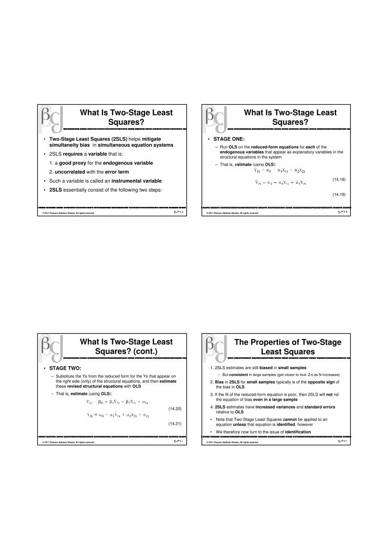
1-٣٦٨© 2011 Pearson Addison-Wesley. All rights reserved.

What Is Two-Stage Least Squares?

• Two-Stage Least Squares (2SLS) helps mitigate simultaneity bias in simultaneous equation systems

• 2SLS requires a variable that is:

1. a good proxy for the endogenous variable

2. uncorrelated with the error term

• Such a variable is called an instrumental variable

• 2SLS essentially consist of the following two steps:

1-٣٦٩© 2011 Pearson Addison-Wesley. All rights reserved.

What Is Two-Stage Least Squares?

• STAGE ONE:

– Run OLS on the reduced-form equations for each of the endogenous variables that appear as explanatory variables in the structural equations in the system

– That is, estimate (using OLS):

(14.18)

(14.19)

1-٣٧٠© 2011 Pearson Addison-Wesley. All rights reserved.

What Is Two-Stage Least Squares? (cont.)

• STAGE TWO:

– Substitute the Ys from the reduced form for the Ys that appear on the right side (only) of the structural equations, and then estimate

these revised structural equations with OLS

– That is, estimate (using OLS):

(14.20)

(14.21)

1-٣٧١© 2011 Pearson Addison-Wesley. All rights reserved.

The Properties of Two-Stage Least Squares

1. 2SLS estimates are still biased in small samples

– But consistent in large samples (get closer to true βs as N increases)

2. Bias in 2SLS for small samples typically is of the opposite sign of the bias in OLS

3. If the fit of the reduced-form equation is poor, then 2SLS will not rid the equation of bias even in a large sample

4. 2SLS estimates have increased variances and standard errors

relative to OLS

• Note that Two-Stage Least Squares cannot be applied to an equation unless that equation is identified, however

• We therefore now turn to the issue of identification

1-٣٧٢© 2011 Pearson Addison-Wesley. All rights reserved.

What Is the Identification Problem?

• Identification is a precondition for the application of 2SLS to equations in simultaneous systems

• A structural equation is identified only when enough of the system’s predetermined variables are omitted from the equation in question to allow that equation to be distinguished from all the others in the system

– Note that one equation in a simultaneous system might be identified and another might not

• Most simultaneous systems are fairly complicated, so econometricians need a general method by which to determine whether equations are identified

• The method typically used is the order condition of identification, to which we now turn

1-٣٧٣© 2011 Pearson Addison-Wesley. All rights reserved.

The Order Condition of Identification

• Is a systematic method of determining whether a particular equation in a simultaneous system has the potential to be identified

• If an equation can meet the order condition, then it is almost always identified

• We thus say that the order condition is a necessary but not sufficient condition of identification

1-٣٧٤© 2011 Pearson Addison-Wesley. All rights reserved.

The Order Condition of Identification (cont.)

• THE ORDER CONDITION:

– A necessary condition for an equation to be identified is that the number of predetermined (exogenous plus lagged

endogenous) variables in the system be greater than or

equal to the number of slope coefficients in the equation of interest

• Or, in equation form, a structural equation meets the order condition if:

# predetermined variables ≥ # slope coefficients

(in the simultaneous system) (in the equation)

1-٣٧٥© 2011 Pearson Addison-Wesley. All rights reserved.

Figure 14.1 Supply and Demand Simultaneous Equations

1-٣٧٦© 2011 Pearson Addison-Wesley. All rights reserved.

Figure 14.3A Shifting Supply Curve

1-٣٧٧© 2011 Pearson Addison-Wesley. All rights reserved.

Figure 14.4When Both Curves Shift

1-٣٧٨© 2011 Pearson Addison-Wesley. All rights reserved.

Table 14.1aData for a Small Macromodel

1-٣٧٩© 2011 Pearson Addison-Wesley. All rights reserved.

Table 14.1bData for a Small Macromodel

1-٣٨٠© 2011 Pearson Addison-Wesley. All rights reserved.


• Endogenous variable

• Predetermined variable

• Structural equation

• Reduced-form equation

• Simultaneity bias

• Two-Stage Least Squares

• Identification

• Order condition for identification

1-٣٨١© 2011 Pearson Addison-Wesley. All rights reserved.

Chapter 15

Forecasting

1-٣٨٢© 2011 Pearson Addison-Wesley. All rights reserved.

What Is Forecasting?

• In general, forecasting is the act of predicting the future

• In econometrics, forecasting is the estimation of the expected value of a dependent variable for observations that are not part of the same

data set

• In most forecasts, the values being predicted are for time periods in

the future, but cross-sectional predictions of values for countries or people not in the sample are also common

• To simplify terminology, the words prediction and forecast will be used interchangeably in this chapter

– Some authors limit the use of the word forecast to out-of-sample prediction for a time series

1-٣٨٣© 2011 Pearson Addison-Wesley. All rights reserved.

What Is Forecasting? (cont.)

• Econometric forecasting generally uses a single linear equation to predict or forecast

• Our use of such an equation to make a forecast can be summarized into two steps:

1. Specify and estimate an equation that has as its dependent variable the item that we wish to forecast:

(15.2)

1-٣٨٤© 2011 Pearson Addison-Wesley. All rights reserved.

What Is Forecasting? (cont.)

2. Obtain values for each of the independent variables for the observations for which we want a forecast and substitute them into our forecasting equation:

(15.3)

• Figure 15.1 illustrates two examples

1-٣٨٥© 2011 Pearson Addison-Wesley. All rights reserved.

Figure 15.1a Forecasting Examples

1-٣٨٦© 2011 Pearson Addison-Wesley. All rights reserved.

Figure 15.1b Forecasting Examples

1-٣٨٧© 2011 Pearson Addison-Wesley. All rights reserved.

More Complex Forecasting Problems

• The forecasts generated in the previous section are quite simple, however, and most actual forecasting involves one or more additional questions—for example:

1. Unknown Xs: It is unrealistic to expect to know the values for the independent variables outside the sample

• What happens when we don’t know the values of the independent variables for the forecast period?

2. Serial Correlation: If there is serial correlation involved, the forecasting equation may be estimated with GLS

• How should predictions be adjusted when forecasting equations are estimated with GLS?

1-٣٨٨© 2011 Pearson Addison-Wesley. All rights reserved.

More Complex Forecasting Problems (cont.)

3. Confidence Intervals: All the previous forecasts were single values, but such single values are almost never exactly right, so maybe it would be more helpful if we forecasted a confidence interval instead

• How can we develop these confidence intervals?

4. Simultaneous Equations Models: As we saw in Chapter 14, many economic and business equations are part of simultaneous models

• How can we use an independent variable to forecast a dependent variable when we know that a change in value of the dependent variable will change, in turn, the value of the independent variable that we used to make the forecast?

1-٣٨٩© 2011 Pearson Addison-Wesley. All rights reserved.

Conditional Forecasting (Unknown X Values for the Forecast Period)

• Unconditional forecast: all values of the independent variables are known with certainty

– This is rare in practice

• Conditional forecast: actual values of one or more of the independent variables are not known

– This is the more common type of forecast

1-٣٩٠© 2011 Pearson Addison-Wesley. All rights reserved.

Conditional Forecasting (Unknown X Values for the Forecast Period) (cont.)

• The careful selection of independent variables can sometimes help avoid the need for conditional forecasting

• This opportunity can arise when the dependent variable can be expressed as a function of leading indicators:

– A leading indicator is an independent variable the movements of which anticipate movements in the dependent variable

– The best known leading indicator, the Index of Leading

Economic Indicators, is produced each month

1-٣٩١© 2011 Pearson Addison-Wesley. All rights reserved.

Forecasting with Serially Correlated Error Terms

• Recall from Chapter 9 that when serial correlation is severe, one remedy is to run Generalized Least Squares (GLS) as noted in Equation 9.18:

(9.18)

• If Equation 9.18 is estimated, the dependent variable will be:

(15.7)

• Thus, if a GLS equation is used for forecasting, it will producepredictions of Y*T + 1 rather than of YT+1

• Such predictions thus will be of the wrong variable!

1-٣٩٢© 2011 Pearson Addison-Wesley. All rights reserved.

Forecasting with Serially Correlated Error Terms (cont.)

• If forecasts are to be made with a GLS equation, Equation 9.18 should first be solved for YT before forecasting is attempted:

(15.8)

• Next, substitute T+1 for t (to forecast time period T+1) and insert estimates for the coefficients, ρs and Xs into the equation to get:

(15.9)

• Equation 15.9 thus should be used for forecasting when an equation has been estimated with GLS to correct for serial correlation

1-٣٩٣© 2011 Pearson Addison-Wesley. All rights reserved.

Forecasting Confidence Intervals

• The techniques we use to test hypotheses can also be adapted to create forecasting confidence intervals

• Given a point forecast, all we need to generate a confidence interval around that forecast are tc, the critical t-value (for the desired level of confidence), and SF, the estimated standard error of the forecast:

(15.11)

• The critical t-value, tc, can be found in Statistical Table B-1 (for a two-tailed test with T-K-1 degrees of freedom)

1-٣٩٤© 2011 Pearson Addison-Wesley. All rights reserved.

Forecasting Confidence Intervals (cont.)

• Lastly, the standard error of the forecast, SF, for an equation with just one independent variable, equals the square root of the forecast error variance:

(15.13)

where:

s2 = the estimated variance of the error term

T = the number of observations in the sample

XT+1 = the forecasted value of the single independent variable

= the arithmetic mean of the observed Xs in the sample

• Figure 15.2 illustrates an example of a forecast confidence interval

X

1-٣٩٥© 2011 Pearson Addison-Wesley. All rights reserved.

Figure 15.2 A Confidence Interval for

1-٣٩٦© 2011 Pearson Addison-Wesley. All rights reserved.

Forecasting with Simultaneous Equations Systems

• How should forecasting be done in the context of a simultaneous model?

• There are two approaches to answering this question, depending on whether there are lagged endogenous variables on the right-hand side of any of the equations in the system:

1-٣٩٧© 2011 Pearson Addison-Wesley. All rights reserved.

Forecasting with Simultaneous Equations Systems (cont.)

1. No lagged endogenous variables in the system:

• the reduced-form equation for the particular endogenous variable can be used for forecasting because it represents the simultaneous solution of the system for the endogenous variable being forecasted

2. Lagged endogenous variables in the system:

• then the approach must be altered to take into account the dynamic

interaction caused by the lagged endogenous variables

• For simple models, this sometimes can be done by substitutingfor the lagged endogenous variables where they appear in the reduced-form equations

• If such a manipulation is difficult, however, then a technique called simulation analysis can be used

1-٣٩٨© 2011 Pearson Addison-Wesley. All rights reserved.

ARIMA Models

• ARIMA is a highly refined curve-fitting device that uses current and past values of the dependent variable to produce often accurate short-term forecasts of that variable

– Examples of such forecasts are stock market price predictions created by brokerage analysts (called “chartists” or “technicians”) based entirely on past patterns of movement of the stock prices

• If ARIMA models thus essentially ignores economic theory (by ignoring “traditional” explanatory variables), why use them?

• The use of ARIMA is appropriate when:

– little or nothing is known about the dependent variable being forecasted,

– the independent variables known to be important cannot be forecasted effectively

– all that is needed is a one or two-period forecast1-٣٩٩© 2011 Pearson Addison-Wesley. All rights reserved.

ARIMA Models (cont.)

• The ARIMA approach combines two different specifications (called processes) into one equation:

1. An autoregressive process (AR):

• expresses a dependent variable as a function of past values of the dependent variable

• This is similar to the serial correlation error term function of Chapter 9 and to the dynamic model of Chapter 12

2. a moving average process (MA):

• expresses a dependent variable as a function of past values of the error term

• Such a function is a moving average of past error term observations that can be added to the mean of Y to obtain a moving average of past values of Y

1-٤٠٠© 2011 Pearson Addison-Wesley. All rights reserved.


• To create an ARIMA model, we begin with an econometric equation with no independent variables:

• and then add to it both the autoregressive and moving-average processes:

(15.17)

where the θs and the φs are the coefficients of the autoregressive

and moving-average processes, respectively, and p and q are the number of past values used of Y and ε, respectively

1-٤٠١© 2011 Pearson Addison-Wesley. All rights reserved.


• Before this equation can be applied to a time series, however, it must be ensured that the time series is stationary, as defined in Section 12.4

• For example, a non-stationary series can often be converted

into a stationary one by taking the first difference:

(15.18)

• If the first differences do not produce a stationary series, then first differences of this first-differenced series can be taken—i.e. a second-difference transformation:

(15.19)

1-٤٠٢© 2011 Pearson Addison-Wesley. All rights reserved.


• If a forecast of Y* or Y** is made, then it must be converted back into

Y terms

• For example, if d = 1 (where d is the number of differences taken to make Y stationary), then:

(15.20)

• This conversion process is similar to integration in mathematics, so the “I” in ARIMA stands for “integrated”

• ARIMA thus stands for Auto-Regressive Integrated Moving Average

– An ARIMA model with p, d, and q specified is usually denoted as ARIMA (p,d,q) with the specific integers chosen inserted for p, d, and q

– If the original series is stationary and d therefore equals 0, this is sometimes shortened to ARMA

1-٤٠٣© 2011 Pearson Addison-Wesley. All rights reserved.


• Unconditional forecast

• Conditional forecast

• Leading indicator

• Confidence interval (of forecast)

• Autoregressive process

• Moving-average process

• ARIMA(p,d,q)

1-٤٠٤© 2011 Pearson Addison-Wesley. All rights reserved.

Chapter 16

Experimental and Panel Data

1-٤٠٥© 2011 Pearson Addison-Wesley. All rights reserved.

Random Assignment Experiments

• When medical researchers want to examine the effect of a new drug, they use an experimental design called an random assignment experiment

• In such experiments, two groups are chosen randomly:

1. Treatment group: receives the treatment (a specific medicine, say)

2. Control group: receives a harmless, ineffective placebo

• The resulting equation is:

OUTCOMEi = β0 + β1TREATMENTi + εi (16.1)

where:

OUTCOMEi = a measure of the desired outcome in the ith individual

TREATMENTi = a dummy variable equal to 1 for individuals in the treatment group and 0 for individuals in the control group

1-٤٠٦© 2011 Pearson Addison-Wesley. All rights reserved.

Random Assignment Experiments (cont.)

• But random assignment can’t always control for all possible other factors—though sometimes we may be able to identify some of these factors and add them to our equation

• Let’s say that the treatment is job training:

– Suppose that random assignment, by chance, results in one group having more males and being slightly older than the other group

– If gender and age matter in determining earnings, then we can control for the different composition of the two groups by including gender and age in our regression equation:

OUTCOMEi = β0 + β1TREATMENTi + β2X1i + β3X2i + εi (16.2)

where: X1 = dummy variable for the individual’s gender

X2 = the individual’s age

1-٤٠٧© 2011 Pearson Addison-Wesley. All rights reserved.


• Unfortunately, random assignment experiments are not common in economics because they are subject to problems that typically do not plague medical experiments—e.g.:

1. Non-Random Samples:

• Most subjects in economic experiments are volunteers, and samples of volunteers often aren’t random and therefore may not be representative of the overall population

• As a result, our conclusions may not apply to everyone

2. Unobservable Heterogeneity:

• In Equation 16.2, we added observable factors to the equation to avoid omitted variable bias, but not all omitted factors in economics are observable

• This “unobservable omitted variable” problem is called unobserved

heterogeneity

1-٤٠٨© 2011 Pearson Addison-Wesley. All rights reserved.


3. The Hawthorne Effect:

• Human subjects typically know that they’re being studied, and they usually know whether they’re in the treatment group or the control group

• The fact that human subjects know that they’re being observed sometimes can change their behavior, and this change in behavior could

clearly change the results of the experiment

4. Impossible Experiments:

• It’s often impossible (or unethical) to run a random assignment experiment in economics

• Think about how difficult it would be to use a random assignmentexperiment to study the impact of marriage on earnings!

1-٤٠٩© 2011 Pearson Addison-Wesley. All rights reserved.

Natural Experiments

• Natural experiments (or quasi-experiments) are similar to random assignment experiments, except:

– observations fall into treatment and control groups “naturally” (because of an exogenous event) instead of being randomly assigned by the researcher

– By “exogenous event” is meant that the natural event must not be under the control of either of the two groups

1-٤١٠© 2011 Pearson Addison-Wesley. All rights reserved.

Natural Experiments (cont.)

• The appropriate regression equation for such a natural experiment is:ΔOUTCOMEi = β0 + β1TREATMENTi + β2X1i + β3X2i + εi (16.3)

where:ΔOUTCOMEi is defined as the outcome after the treatment minus the outcome before the treatment for the ith observationβ1 is called the difference-in-differences estimator, and it measures the difference between the change in the treatment group and the change in the control group, holding constant X1 and X2

• Figure 16.1 illustrates an example of a natural experiment

1-٤١١© 2011 Pearson Addison-Wesley. All rights reserved.

Figure 16.1 Treatment and Control Groups for Los Angeles

1-٤١٢© 2011 Pearson Addison-Wesley. All rights reserved.

What Are Panel Data?

• Panel (or longitudinal) data combine time-series and cross-

sectional data such that observations on the same variables from the same cross sectional sample are followed over two or more different time periods

• Why use panel data? At least three reasons—using panel data:

1. certainly will increase sample sizes!

2. can help provide insights into analytical questions that can’t be

answered by using time-series or cross-sectional data alone:

• Allows determining whether the same people are unemployed year after year or whether different individuals are unemployed in different years

3. often allow researchers to avoid omitted variable problems that otherwise would cause bias in cross-sectional studies

1-٤١٣© 2011 Pearson Addison-Wesley. All rights reserved.

What Are Panel Data? (cont.)

• There are four different kinds of variables that we encounter when we use panel data:

1. Variables that can differ between individuals but don’t change

over time:

• e.g., gender, ethnicity, and race

2. Variables that change over time but are the same for all

individuals in a given time period:

• e.g., the retail price index and the national unemployment rate

3. Variables that vary both over time and between individuals:

• e.g., income and marital status

4. Trend variables that vary in predictable ways:

• e.g., an individual’s age

1-٤١٤© 2011 Pearson Addison-Wesley. All rights reserved.

The Fixed Effects Model

• There are several alternative panel data estimation procedures

• Most researchers use the fixed effects model, which allows each cross-sectional unit to have a different intercept:

Yit = β0 + β1Xit + β2D2i + ... + βNDNi + vit (16.4)

where:

D2 = intercept dummy equal to 1 for the second cross-sectional entity and 0 otherwise

DN = intercept dummy equal to 1 for the Nth cross-sectional entity and 0 otherwise

• Note that Y, X, and v have two subscripts!

1-٤١٥© 2011 Pearson Addison-Wesley. All rights reserved.

The Fixed Effects Model (cont.)

• One major advantage of the fixed effects model is that it avoids bias

due to omitted variables that don’t change over time

– e.g., race or gender

– Such time-invariant omitted variables often are referred to as unobserved

heterogeneity or a fixed effect

• To understand how this works, consider what Equation 16.4 would look like with only two years worth of data:

Yit = β0 + β1Xit + β2D2i + vit (16.5)

• Let’s decompose the error term, vit, into two components, a classical error term (εit) and the unobserved impact of the time-invariant

omitted variables (ai):

vit = εit + ai (16.6)

1-٤١٦© 2011 Pearson Addison-Wesley. All rights reserved.


• If we substitute Equation 16.6 into Equation 16.5, we get:

Yit = β0 + β1Xit + β2D2i + εit + ai (16.7)

• Next, average Equation 16.7 over time for each observation i, thus producing:

Yi = β0 + β1Xi + β2D2i + εi + ai (16.8)

where the bar over a variable indicates the mean of that variable across time

• Note that ai, β2D2i, and β0 don’t have bars over them because they’re constant over time

1-٤١٧© 2011 Pearson Addison-Wesley. All rights reserved.


• If we now subtract Equation 16.8 from Equation 16.7, we get:

• Note that ai, β2, D2i, and β0 are subtracted out because they’re in both equations

• We’ve therefore shown that estimating panel data with the fixed effects model does indeed drop the ai out of the equation

• Hence, the fixed effects model will not experience bias due to time-

invariant omitted variables!

• Example: The death penalty and the murder rate:

– Figures 16.2 and 16.3 illustrates the importance of the fixed-effects model: the unlikely (positive) result from the cross-section model is reversed by the fixed effects model!

1-٤١٨© 2011 Pearson Addison-Wesley. All rights reserved.

Figure 16.2 In a Single-Year Cross-Sectional Model, the Murder Rate

Appears to Increase with Executions

1-٤١٩© 2011 Pearson Addison-Wesley. All rights reserved.

Figure 16.3 In a Panel Data Model, the Murder Rate Decreases with Executions

1-٤٢٠© 2011 Pearson Addison-Wesley. All rights reserved.

The Random Effects Model

• Recall that the fixed effects model is based on the assumption that each cross-sectional unit has its own intercept

• The random effects model instead is based on the assumption that the intercept for each cross-sectional unit is drawn from

a distribution (that is centered around a mean intercept)

• Thus each intercept is a random draw from an “intercept distribution” and therefore is independent of the error term for any particular observation

– Hence the term random effects model

1-٤٢١© 2011 Pearson Addison-Wesley. All rights reserved.

The Random Effects Model (cont.)

• Advantages of the random effects model:

1. more degrees of freedom than a fixed effects model

• This is because rather than estimating an intercept for virtually every cross-sectional unit, all we need to do is to estimate the parameters that describe the distribution of the intercepts.

2. Can now also estimate time-invariant explanatory variables(like race or gender).

• Disadvantages of the random effects model:

1. Most importantly, the random effects estimator requires us to assume that ai is uncorrelated with the independent variables, the Xs, if we’re going to avoid omitted variable bias

• This may be an overly strong assumption in many cases

1-٤٢٢© 2011 Pearson Addison-Wesley. All rights reserved.

Choosing Between Fixed and Random Effects

• One key is the nature of the relationship between ai and the Xs:

– If they’re likely to be correlated, then it makes sense to use the fixed effects model

– If not, then it makes sense to use the random effects model

• Can also use the Hausman test to examine whether there is correlation between ai and X

• Essentially, this procedure tests to see whether the regression coefficients under the fixed effects and random effects models are statistically different from each other

– If they are different, then the fixed effects model is preferred

– If the they are not different, then the random effects model is preferred(or estimates of both the fixed effects and random effects models are provided)

1-٤٢٣© 2011 Pearson Addison-Wesley. All rights reserved.

Table 16.1a

1-٤٢٤© 2011 Pearson Addison-Wesley. All rights reserved.

Table 16.1b

1-٤٢٥© 2011 Pearson Addison-Wesley. All rights reserved.

Table 16.1c

1-٤٢٦© 2011 Pearson Addison-Wesley. All rights reserved.

Table 16.1d

1-٤٢٧© 2011 Pearson Addison-Wesley. All rights reserved.

Table 16.1e

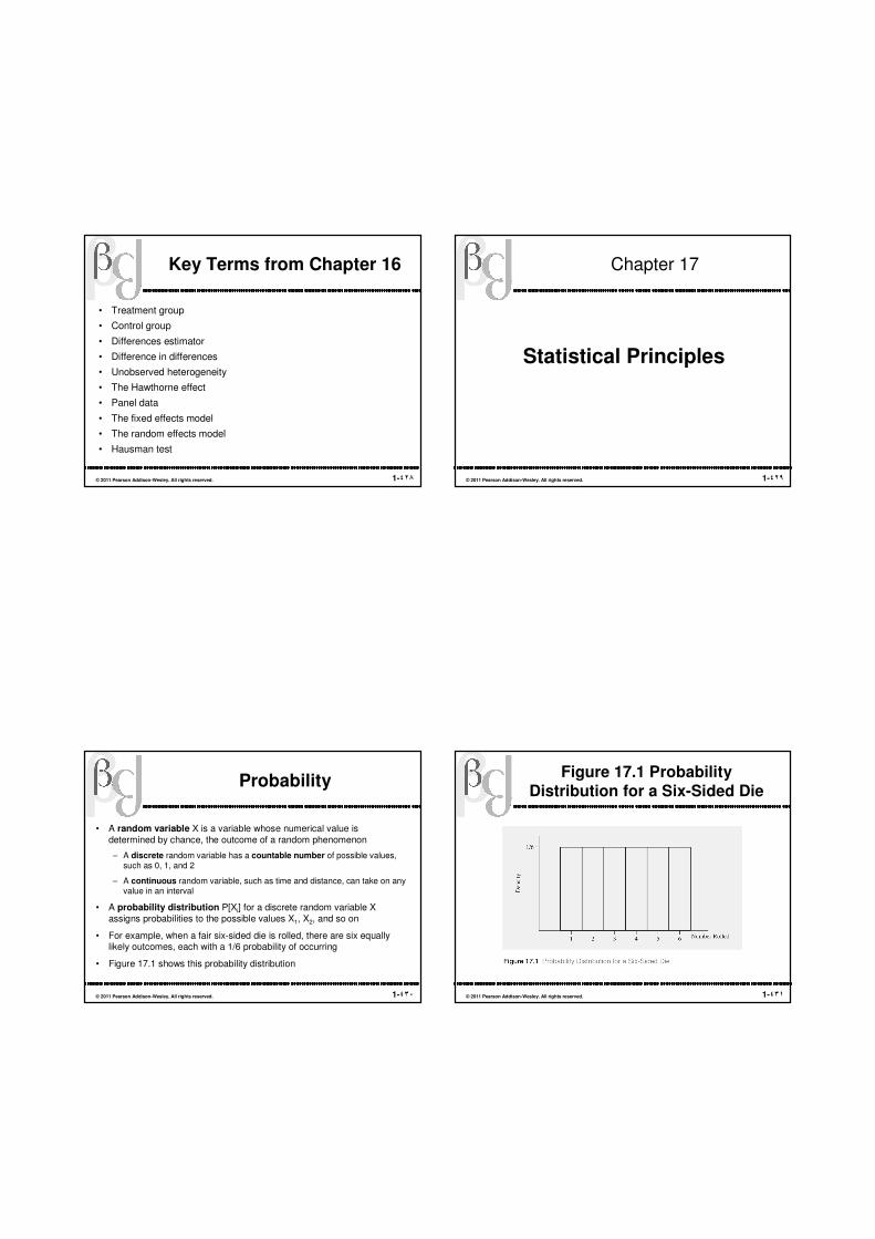
1-٤٢٨© 2011 Pearson Addison-Wesley. All rights reserved.


• Treatment group

• Control group

• Differences estimator

• Difference in differences

• Unobserved heterogeneity

• The Hawthorne effect

• Panel data

• The fixed effects model

• The random effects model

• Hausman test

1-٤٢٩© 2011 Pearson Addison-Wesley. All rights reserved.

Chapter 17

Statistical Principles

1-٤٣٠© 2011 Pearson Addison-Wesley. All rights reserved.

Probability

• A random variable X is a variable whose numerical value is determined by chance, the outcome of a random phenomenon

– A discrete random variable has a countable number of possible values, such as 0, 1, and 2

– A continuous random variable, such as time and distance, can take on any value in an interval

• A probability distribution P[Xi] for a discrete random variable X assigns probabilities to the possible values X1, X2, and so on

• For example, when a fair six-sided die is rolled, there are six equally likely outcomes, each with a 1/6 probability of occurring

• Figure 17.1 shows this probability distribution

1-٤٣١© 2011 Pearson Addison-Wesley. All rights reserved.

Figure 17.1 Probability Distribution for a Six-Sided Die

1-٤٣٢© 2011 Pearson Addison-Wesley. All rights reserved.

Mean, Variance, and Standard Deviation

• The expected value (or mean) of a discrete random variable X is a weighted average of all possible values of X, using the probability of each X value as weights:

(17.1)

• the variance of a discrete random variable X is a weighted average, for all possible values of X, of the squared difference between X and its expected value, using the probability of each X value as weights:

(17.2)

• The standard deviation σ is the square root of the variance

µ = E[X] = X

iP[X

i]

i

∑

σ2 = E[(X − µ)2 ] = (X

i− µ)2P[X

i]

i

∑

1-٤٣٣© 2011 Pearson Addison-Wesley. All rights reserved.

Continuous Random Variables

• Our examples to this point have involved discrete random variables, for which we can count the number of possible outcomes:

– The coin can be heads or tails; the die can be 1, 2, 3, 4, 5, or 6

• For continuous random variables, however, the outcome can be any

value in a given interval

– For example, Figure 17.2 shows a spinner for randomly selecting a point on a circle

• A continuous probability density curve shows the probability that the outcome is in a specified interval as the corresponding area under the curve

– This is illustrated for the case of the spinner in Figure 17.3

1-٤٣٤© 2011 Pearson Addison-Wesley. All rights reserved.

Figure 17.2 Pick a Number, Any Number

1-٤٣٥© 2011 Pearson Addison-Wesley. All rights reserved.

Figure 17.3 A Continuous Probability Distribution for the Spinner

1-٤٣٦© 2011 Pearson Addison-Wesley. All rights reserved.

Standardized Variables

• To standardize a random variable X, we subtract its mean and then divide by its standard deviation :

(17.3)

• No matter what the initial units of X, the standardized random variable Z has a mean of 0 and a standard deviation of 1

• The standardized variable Z measures how many standard deviations X is above or below its mean:

– If X is equal to its mean, Z is equal to 0

– If X is one standard deviation above its mean, Z is equal to 1

– If X is two standard deviations below its mean, Z is equal to –2

• Figures 17.4 and 17.5 illustrates this for the case of dice and fair coin flips, respectively

Z =

X − µ

σ

1-٤٣٧© 2011 Pearson Addison-Wesley. All rights reserved.

Figure 17.4a Probability Distribution for Six-Sided Dice, Using Standardized Z

1-٤٣٨© 2011 Pearson Addison-Wesley. All rights reserved.

Figure 17.4b Probability Distribution for Six-Sided Dice, Using Standardized Z

1-٤٣٩© 2011 Pearson Addison-Wesley. All rights reserved.

Figure 17.4c Probability Distribution for Six-Sided Dice, Using Standardized Z

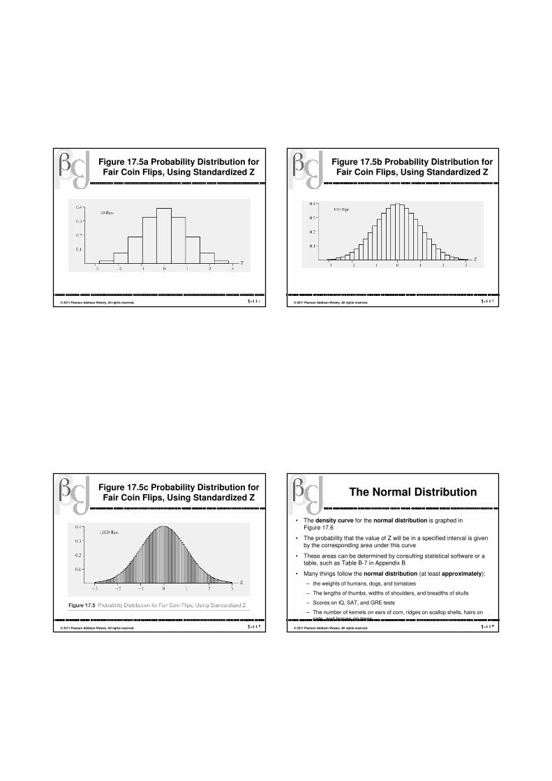
1-٤٤٠© 2011 Pearson Addison-Wesley. All rights reserved.

Figure 17.5a Probability Distribution for Fair Coin Flips, Using Standardized Z

1-٤٤١© 2011 Pearson Addison-Wesley. All rights reserved.

Figure 17.5b Probability Distribution for Fair Coin Flips, Using Standardized Z

1-٤٤٢© 2011 Pearson Addison-Wesley. All rights reserved.

Figure 17.5c Probability Distribution for Fair Coin Flips, Using Standardized Z

1-٤٤٣© 2011 Pearson Addison-Wesley. All rights reserved.

The Normal Distribution

• The density curve for the normal distribution is graphed in Figure 17.6

• The probability that the value of Z will be in a specified interval is given by the corresponding area under this curve

• These areas can be determined by consulting statistical software or a table, such as Table B-7 in Appendix B

• Many things follow the normal distribution (at least approximately):

– the weights of humans, dogs, and tomatoes

– The lengths of thumbs, widths of shoulders, and breadths of skulls

– Scores on IQ, SAT, and GRE tests

– The number of kernels on ears of corn, ridges on scallop shells, hairs on cats, and leaves on trees

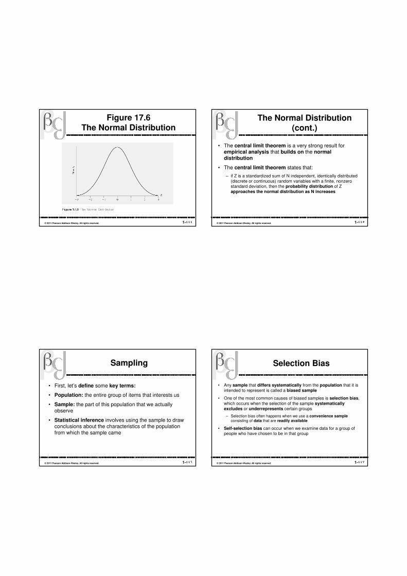
1-٤٤٤© 2011 Pearson Addison-Wesley. All rights reserved.

Figure 17.6 The Normal Distribution

1-٤٤٥© 2011 Pearson Addison-Wesley. All rights reserved.

The Normal Distribution (cont.)

• The central limit theorem is a very strong result for empirical analysis that builds on the normal distribution

• The central limit theorem states that:

– if Z is a standardized sum of N independent, identically distributed (discrete or continuous) random variables with a finite, nonzerostandard deviation, then the probability distribution of Z approaches the normal distribution as N increases

1-٤٤٦© 2011 Pearson Addison-Wesley. All rights reserved.

Sampling

• First, let’s define some key terms:

• Population: the entire group of items that interests us

• Sample: the part of this population that we actually observe

• Statistical inference involves using the sample to draw conclusions about the characteristics of the population from which the sample came

1-٤٤٧© 2011 Pearson Addison-Wesley. All rights reserved.

Selection Bias

• Any sample that differs systematically from the population that it is intended to represent is called a biased sample

• One of the most common causes of biased samples is selection bias, which occurs when the selection of the sample systematically

excludes or underrepresents certain groups

– Selection bias often happens when we use a convenience sampleconsisting of data that are readily available

• Self-selection bias can occur when we examine data for a group of people who have chosen to be in that group

1-٤٤٨© 2011 Pearson Addison-Wesley. All rights reserved.

Survivor and Nonresponse Bias

• A retrospective study looks at past data for a contemporaneously selected sample

– for example, an examination of the lifetime medical records of 65-year-olds

• A prospective study, in contrast, selects a sample and then tracks the members over time

• By its very design, retrospective studies suffer from survivor bias: we necessarily exclude members of the past population who are no longer around!

• Nonresponse bias: The systematic refusal of some groups to

participate in an experiment or to respond to a poll

1-٤٤٩© 2011 Pearson Addison-Wesley. All rights reserved.

The Power of Random Selection

• In a simple random sample of size N from a given population:

– each member of the population is equally likely to be included in the sample

– every possible sample of size N from this population has an equal chance of being selected

• How do we actually make random selections?

• We would like a procedure that is equivalent to the following:

– put the name of each member of the population on its own slip of paper

– drop these slips into a box

– mix thoroughly

– pick members out randomly

• In practice, random sampling is usually done through some sort of numerical identification combined with a computerized random selection of numbers

1-٤٥٠© 2011 Pearson Addison-Wesley. All rights reserved.

Estimation

• First, some terminology:

• Parameter: a characteristic of the population whose value is unknown, but can be estimated

• Estimator: a sample statistic that will be used to estimate the value of the population parameter

• Estimate: the specific value of the estimator that is obtained in one particular sample

• Sampling variation: the notion that because samples are chosen randomly, the sample average will vary from sample to sample, sometimes being larger than the population mean and sometimes lower

1-٤٥١© 2011 Pearson Addison-Wesley. All rights reserved.

Sampling Distributions

• The sampling distribution of a statistic is the probability distribution

or density curve that describes the population of all possible valuesof this statistic

– For example, it can be shown mathematically that if the individual observations are drawn from a normal distribution, then the sampling distribution for the sample mean is also normal

– Even if the population does not have a normal distribution, the sampling distribution of the sample mean will approach a normal distribution as the sample size increases

• It can be shown mathematically that the sampling distribution for the sample mean has the following mean and standard deviation:

(17.5) Mean of X = µ

Standard deviation of X = µ / N

1-٤٥٢© 2011 Pearson Addison-Wesley. All rights reserved.

The Mean of the Sampling Distribution

• A sample statistic is an unbiased estimator of a population parameter if the mean of the sampling distribution of this statistic is equal to the value of the population parameter

• Because the mean of the sampling distribution of X is μ, X is an unbiased estimator of μ

1-٤٥٣© 2011 Pearson Addison-Wesley. All rights reserved.

The Standard Deviation of the Sampling Distribution

• One way of gauging the accuracy of an estimator is with its standard deviation:

– If an estimator has a large standard deviation, there is a substantial probability that an estimate will be far from its mean

– If an estimator has a small standard deviation, there is a high probability that an estimate will be close to its mean

1-٤٥٤© 2011 Pearson Addison-Wesley. All rights reserved.

The t-Distribution

• When the mean of a sample from a normal distribution is standardized by subtracting the mean of its sampling distribution and dividing by the standard deviation of its sampling distribution, the resulting Z variable

has a normal distribution

• W.S. Gosset determined (in 1908) the sampling distribution of the variable that is created when the mean of a sample from a normaldistribution is standardized by subtracting and dividing by itsstandard error (≡ the standard deviation of an estimator):

1-٤٥٥© 2011 Pearson Addison-Wesley. All rights reserved.

The t-Distribution (cont.)

• The exact distribution of t depends on the sample size,

– as the sample size increases, we are increasingly confident of the accuracy of the estimated standard deviation

• Table B-1 at the end of the textbook shows some probabilities for various t-distributions that are identified by the number of degrees of freedom:

degrees of freedom = # observations - # estimated parameters

1-٤٥٦© 2011 Pearson Addison-Wesley. All rights reserved.

Confidence Intervals

• A confidence interval measures the reliability of a given statistic such as X

• The general procedure for determining a confidence interval for a population mean can be summarized as:

1. Calculate the sample average X

2. Calculate the standard error of X by dividing the sample standard deviation s by the square root of the sample size N

3. Select a confidence level (such as 95 percent) and look in Table B-1 with N-1 degrees of freedom to determine the t-value that corresponds to this probability

4. A confidence interval for the population mean is then given by:

X ± t * s / N

1-٤٥٧© 2011 Pearson Addison-Wesley. All rights reserved.

Sampling from Finite Populations

• Notably, a confidence interval does not depend on the size of the population

• This may first seem surprising: if we are trying to estimate a characteristic of a large population, then wouldn’t we also need a large sample?

• The reason why the size of the population doesn’t matter is that the chances that the luck of the draw will yield a sample whose meandiffers substantially from the population mean depends on the size of the sample and the chances of selecting items that are far from the population mean

– That is, not on how many items there are in the population

1-٤٥٨© 2011 Pearson Addison-Wesley. All rights reserved.


• Random variable

• Probability distribution

• Expected Value

• Mean

• Variance

• Standard deviation

• Standardized random variable

• Population

• Sample

• Selection, survivor, and nonresponse bias

• Sampling distribution

• Population mean

• Sample mean

• Population standard deviation

• Sample standard deviation


• Confidence interval

Econometrics and Quantitative Chapter 1site.iugaza.edu.ps/ssafi/files/2012/09/Lectures-20121.pdf ·...

Documents

Transcript of Econometrics and Quantitative Chapter 1site.iugaza.edu.ps/ssafi/files/2012/09/Lectures-20121.pdf ·...