Econometrica,Vol.70,No.1(January,2002),223–262yacine/mle.pdf · Cii=0 4, and D0such that for...

Econometrica, Vol. 70, No. 1 (January, 2002), 223–262

MAXIMUM LIKELIHOOD ESTIMATION OF DISCRETELY SAMPLEDDIFFUSIONS: A CLOSED-FORM APPROXIMATION APPROACH

By Yacine Aït-Sahalia1

When a continuous-time diffusion is observed only at discrete dates, in most casesthe transition distribution and hence the likelihood function of the observations is notexplicitly computable. Using Hermite polynomials, I construct an explicit sequence ofclosed-form functions and show that it converges to the true (but unknown) likelihoodfunction. I document that the approximation is very accurate and prove that maximizingthe sequence results in an estimator that converges to the true maximum likelihood esti-mator and shares its asymptotic properties. Monte Carlo evidence reveals that this methodoutperforms other approximation schemes in situations relevant for financial models.

Keywords: Maximum-likelihood estimation, continuous-time diffusion, discrete sam-pling, transition density, Hermite expansion.

1� introduction

Consider a continuous-time parametric diffusion

dXt = ��Xt��dt+�Xt� �dWt(1.1)

where Xt is the state variable, Wt a standard Brownian motion, ��·�· and �·�·are known functions, and � an unknown parameter vector in an open boundedset � ⊂RK . Diffusion processes are widely used in financial models, for instanceto represent the stochastic dynamics of asset returns, exchange rates, interestrates, macroeconomic factors, etc.While the model is written in continuous time, the available data are always

sampled discretely in time. Ignoring the difference can result in inconsistent esti-mators (see, e.g., Merton (1980) and Melino (1994)). A number of econometricmethods have been recently developed to estimate the parameters of (1.1), with-out requiring that a continuous record of observations be available. Some of thesemethods are based on simulations (Gouriéroux, Monfort, and Renault (1993),Gallant and Tauchen (1996)), others on the generalized method of moments(Hansen and Scheinkman (1995), Duffie and Glynn (1997), Kessler and Sorensen

1 I am grateful to David Bates, René Carmona, Freddy Delbaen, Ron Gallant, Lars Hansen, BjarkeJensen, Per Mykland, Peter C. B. Phillips, Rolf Poulsen, Peter Robinson, Chris Rogers, Angel Ser-rat, Chris Sims, George Tauchen, and in particular a co-editor and three anonymous referees forvery helpful comments and suggestions. Robert Kimmel and Ernst Schaumburg provided excellentresearch assistance. This research was supported by an Alfred P. Sloan Research Fellowship and bythe NSF under Grant SBR-9996023. Mathematica code to calculate the closed-form density sequencecan be found at http://www.princeton.edu/∼yacine.

223

224 yacine aït-sahalia

(1999)), nonparametric density-matching (Aït-Sahalia (1996a, 1996b)), nonpara-metric regression for approximate moments (Stanton (1997)), or are Bayesian(Eraker (1997) and Jones (1997)).As in most contexts, provided one trusts the parametric specification (1.1),

maximum-likelihood is the method of choice. The major caveat in the presentcontext is that the likelihood function for discrete observations generated by (1.1)cannot be determined explicitly for most models. Let pX��x�x0� � denote theconditional density of Xt+� = x given Xt = x0 induced by the model (1.1), alsocalled the transition function. Assume that we observe the process at dates �t =i��i= 0� � � � � n�, where �> 0 is fixed.2 Bayes’ rule combined with the Markoviannature of (1.1), which the discrete data inherit, imply that the log-likelihoodfunction has the simple form

�n��≡n∑i=1ln{pX��Xi� �X�i−1��

}�(1.2)

For some of the rare exceptions where pX is available in closed-form, see Wong(1964); in finance, the models of Black and Scholes (1973), Vasicek (1977), Cox,Ingersoll, and Ross (1985), and Cox (1975) all rely on the known closed-formexpressions.If sampling of the process were continuous, the situation would be simpler.

First, the likelihood function for a continuous record can be obtained by meansof a classical absolutely continuous change of measure (see, e.g., Basawa andPrakasa Rao (1980)).3 Second, when the sampling interval goes to zero, expan-sions for the transition function “in small time” are available in the statisti-cal literature (see, e.g., Azencott (1981)). Dacunha-Castelle and Florens-Zmirou(1986) calculate expressions for the transition function in terms of functionalsof a Brownian Bridge. With discrete-time sampling, the available methods tocompute the likelihood function involve either solving numerically the Fokker-Planck-Kolmogorov partial differential equation (see, e.g., Lo (1988)) or simu-lating a large number of sample paths along which the process is sampled veryfinely (see Pedersen (1995) and Santa-Clara (1995)). Neither method producesa closed-form expression to be maximized over �: the criterion function takeseither the form of an implicit solution to a partial differential equation, or a sumover the outcome of the simulations.By contrast, I construct a closed-form sequence p�JX of approximations to the

transition density, hence from (1.2) a sequence ��J n of approximations to the log-likelihood function �n. I also provide empirical evidence that J = 2 or 3 isamply adequate for models that are relevant in finance.4 Since the expression

2 See Section 3.1 for extensions to the cases where the sampling interval � is time-varying and evenpossibly random.3 Note that the continuous-observation likelihood is only defined if the diffusion function is

known.4 In addition, Jensen and Poulsen (1999) have recently completed a comparison of the method of

this paper against four alternatives: a discrete Euler approximation of the continuous-time model

maximum likelihood estimation 225

Notes: This figure reports the average uniform absolute error of various density approximation techniques applied to the Vasicek,Cox-Ingersoll-Ross and Black-Scholes models. “Euler” refers to the discrete-time, continuous-state, first-order Gaussian approxi-mation scheme for the transition density given in equation (5.4); “Binomial Tree” refers to the discrete-time, discrete-state (two)approximation; “Simulations” refers to an implementation of Pedersen (1995)’s simulated-likelihood method; “PDE” refers to thenumerical solution of the Fokker-Planck-Kolmogorov partial differential equation satisfied by the transition density, using the Crank-Nicolson algorithm. For implementation details on the different methods considered, see Jensen and Poulsen (1999).

Figure 1.—Accuracy and speed of different approximation methods for pX .

��J n to be maximized is explicit, the effort involved is minimal, identical to astandard maximum-likelihood problem with a known likelihood function. Exam-ples are contained in a companion paper (Aït-Sahalia (1999)), which provides,for different models, the corresponding expression of p�JX . Besides makingmaximum-likelihood estimation feasible, these closed-form approximations haveother applications in financial econometrics. For instance, they could be used forderivative pricing, for indirect inference (see Gouriéroux, Monfort, and Renault(1993)), which in its simplest version uses an Euler approximation as instrumen-tal model, or for Bayesian inference—basically whenever an expression for thetransition density is required.The paper is organized as follows. Section 2 describes the sequence of den-

sity approximations and proves its convergence. Section 3 studies the propertiesof the resulting maximum-likelihood estimator. In Section 4, I show how to cal-culate in closed-form the coefficients of the approximation and readers primar-ily interested in applying these results to a specific model can go there directly.

(1.1), a binomial tree approximation, the numerical solution of the PDE, and simulation-based meth-ods, all in the context of various specifications and parameter values that are relevant for interestrate and stock return models. To give an idea of the relative accuracy and speed of these approxima-tions, Figure 1 summarizes their main results. As is clear from the figure, the approximation of thetransition function derived here provides a degree of accuracy and speed that is unmatched by anyof the other methods.


Section 5 gives the results of Monte Carlo simulations. Section 6 concludes. Allproofs are in the Appendix.

2� a sequence of expansions of the transition function

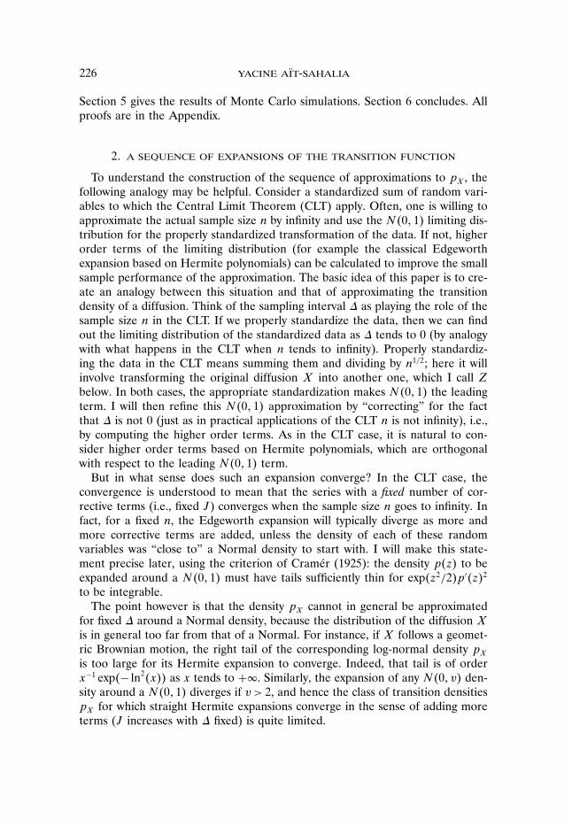
To understand the construction of the sequence of approximations to pX , thefollowing analogy may be helpful. Consider a standardized sum of random vari-ables to which the Central Limit Theorem (CLT) apply. Often, one is willing toapproximate the actual sample size n by infinity and use the N�0�1 limiting dis-tribution for the properly standardized transformation of the data. If not, higherorder terms of the limiting distribution (for example the classical Edgeworthexpansion based on Hermite polynomials) can be calculated to improve the smallsample performance of the approximation. The basic idea of this paper is to cre-ate an analogy between this situation and that of approximating the transitiondensity of a diffusion. Think of the sampling interval � as playing the role of thesample size n in the CLT. If we properly standardize the data, then we can findout the limiting distribution of the standardized data as � tends to 0 (by analogywith what happens in the CLT when n tends to infinity). Properly standardiz-ing the data in the CLT means summing them and dividing by n1/2; here it willinvolve transforming the original diffusion X into another one, which I call Zbelow. In both cases, the appropriate standardization makes N�0�1 the leadingterm. I will then refine this N�0�1 approximation by “correcting” for the factthat � is not 0 (just as in practical applications of the CLT n is not infinity), i.e.,by computing the higher order terms. As in the CLT case, it is natural to con-sider higher order terms based on Hermite polynomials, which are orthogonalwith respect to the leading N�0�1 term.But in what sense does such an expansion converge? In the CLT case, the

convergence is understood to mean that the series with a fixed number of cor-rective terms (i.e., fixed J ) converges when the sample size n goes to infinity. Infact, for a fixed n, the Edgeworth expansion will typically diverge as more andmore corrective terms are added, unless the density of each of these randomvariables was “close to” a Normal density to start with. I will make this state-ment precise later, using the criterion of Cramér (1925): the density p�z to beexpanded around a N�0�1 must have tails sufficiently thin for exp�z2/2p′�z2

to be integrable.The point however is that the density pX cannot in general be approximated

for fixed � around a Normal density, because the distribution of the diffusion Xis in general too far from that of a Normal. For instance, if X follows a geomet-ric Brownian motion, the right tail of the corresponding log-normal density pXis too large for its Hermite expansion to converge. Indeed, that tail is of orderx−1 exp�− ln2�x as x tends to +. Similarly, the expansion of any N�0� v den-sity around a N�0�1 diverges if v > 2, and hence the class of transition densitiespX for which straight Hermite expansions converge in the sense of adding moreterms (J increases with � fixed) is quite limited.


To obtain nevertheless an expansion that converges as more correction termsare added while � remains fixed, I will show that the transformation of thediffusion process X into Z in fact guarantees (unlike the CLT situation) thatthe resulting variable Z has a density pZ that belongs to the class of densitiesfor which the Hermite series converges as more polynomial terms are added.I will then construct a convergent Hermite series for pZ. Since Z is a knowntransformation of X, I will be able to revert the transformation from X to Z andby the Jacobian formula obtain an expansion for the density of X. As a resultof transforming Z back into X, which in general is a nonlinear transformation(unless �x�� is independent of the state variable x), the leading term of theexpansion for the density pX will be a deformed, or stretched, Normal densityrather than the N�0�1 leading term of the expansion for pZ. The rest of thissection makes this basic intuition rigorous. In particular, Theorem 1 will provethat such an expansion converges uniformly to the unknown pX .

2�1� Assumptions and First Transformation X→ Y

I start by making fairly general assumptions on the functions � and . In par-ticular, I do not assume that � and satisfy the typical growth conditions atinfinity, nor do I restrict attention to stationary diffusions only. Let DX = �x� xdenote the domain of the diffusion X. I will consider the two cases whereDX = �−�+ and DX = �0�+. The latter case is often relevant in finance,when considering models for asset prices or nominal interest rates. In addi-tion, the function is often specified in financial models in such a way thatlimx→0+ �x��= 0 and � and/or violate the linear growth conditions near theboundaries. For these reasons, I will devise a set of assumptions where growthconditions (without constraint on the sign of the drift function near the bound-aries) are replaced by assumptions on the sign of the drift near the boundaries(without restriction on the growth of the coefficients). The assumptions are:

Assumption 1 (Smoothness of the Coefficients): The functions ��x�� and�x�� are infinitely differentiable in x, and three times continuously differentiablein �, for all x ∈DX and � ∈�.

Assumption 2 (Non-Degeneracy of the Diffusion):1. If DX = �−�+, there exists a constant c such that �x�� > c > 0 for

all x ∈DX and � ∈�.2. If DX = �0�+� limx→0+ �x�� = 0 is possible, but then there exist con-

stants #0 > 0� $ > 0� % ≥ 0 such that �x�� ≥ $x% for all 0 < x ≤ #0 and � ∈ �.Whether or not limx→0+ �x��= 0, is a nondegenerate on �0�+, that is: foreach # > 0, there exists a constant c# such that �x��≥ c# > 0 for all x ∈ '#�+(and � ∈�.

The first step I employ towards constructing the sequence of approximationsto pX consists in standardizing the diffusion function of X, i.e., transforming X


into Y defined as5

Y ≡ )�X��=∫ X

du/�u��(2.1)

where any primitive of the function 1/ may be selected, i.e., the constant ofintegration is irrelevant. Because > 0 on DX , the function ) is increasing andinvertible for all � ∈ �. It maps DX into DY = �y� y, the domain of Y , wherey ≡ limx→x+ )�x�� and y ≡ limx→x− )�x��. For example, if DX = �0�+ and�x��= x%, then Y = �1−%X1−% if 0< %< 1 (so DY = �0�+, Y = ln�X if%= 1 (so DY = �−�+ and Y =−�%−1X−�%−1 if %> 1 (so DY = �−�0.For a given model under consideration, assume that the parameter space � isrestricted in such a way that DY is independent of � in �. This restriction on �is inessential, but it helps keep the notation simple. By applying Itô’s Lemma, Yhas unit diffusion, that is

dYt = �Y �Yt� �dt+dWt� where(2.2)

�Y �y��=��)−1�y� �� )−1�y� ��

− 12,

,x�)−1�y� ��

Assumption 3 (Boundary Behavior): For all � ∈ ��Y �y�� and its deriva-tives with respect to y and � have at most polynomial growth6 near the bound-aries and limy→y+ or y− -Y �y�� <+ where −-Y is the potential, i.e., -Y �y��≡−��2Y �y��+ ,�Y �y��/,y�/2.

1. Left Boundary: If y = 0, there exist constants .0�/�0 such that for all 0 <y ≤ .0 and � ∈ ��Y �y�� ≥ /y−0 where either 0 > 1 and / > 0, or 0 = 1 and/≥ 1. If y =−, there exist constants E0 > 0 and K > 0 such that for all y ≤−E0and � ∈��Y �y��≥Ky.

2. Right Boundary: If y = +, there exist constants E0 > 0 and K > 0 suchthat for all y ≥E0 and � ∈��Y �y��≤Ky. If y = 0, there exist constants .0�/�0such that for all 0 > y ≥ −.0 and � ∈ ��Y �y�� ≤ −/ �y�−0 where either 0 > 1and / > 0 or 0= 1 and /≥ 1/2.

Note that -Y is not restricted from going to − near the boundaries. Assump-tion 3 is formulated in terms of the function �Y for reasons of convenience, butthe restriction it imposes on the original functions � and follows from (2.1).Assumption 3 only restricts how large �Y can grow if it has the “wrong” sign,meaning that �Y is positive near y and negative near y: then linear growth is themaximum possible rate. But if �Y has the “right” sign, the process is being pulled

5 The same transformation, sometimes referred to as the Lamperti transform, has been used, forinstance, by Florens (1999).6 Define an infinitely differentiable function f as having at most polynomial growth if there exists

an integer p ≥ 0 such that �y � −p�f �y� is bounded above in a neighborhood of infinity. If p = 1� f issaid to have at most linear growth, and if p= 2 at most quadratic growth. Near 0, polynomial growthmeans that �y�+p�f �y� is bounded.


back away from the boundaries and I do not restrict how fast mean-reversionoccurs (up to an arbitrary large polynomial rate for technical reasons). The con-straints on the behavior of the function �Y are essentially the best possible forthe following reasons. If �Y has the wrong sign near an infinity boundary, andgrows faster than linearly, then Y explodes (i.e., can reach the infinity boundary)in finite time. Near a zero boundary, say y = 0, if there exist / > 0 and 0 < 1such that �Y �y�� ≤ ky−0 in a neighborhood of 0+, then 0 becomes attainable.The behavior of the diffusion Y implied by the assumptions made is fully char-acterized by the following proposition, where TY ≡ inf�t ≥ 0 �Yt �∈ DY = �y� y�denotes the exit time from DY :

Proposition 1: Under Assumptions 1–3, (2.2) admits a weak solution �Yt � t ≥0�, unique in probability law, for every distribution of its initial value Y0.7 Theboundaries of DY are unattainable, in the sense that Prob�TY == 1. Finally, if+ is a right boundary, then it is natural if, near +� ��Y �y�� ≤Ky and entranceif �Y �y�� ≤−Ky5 for some 5 > 1. If − is a left boundary, then it is natural if,near −� ��Y �y�� ≤K�y� and entrance if �Y �y��≥K�y�5 for some 5 > 1. If 0is a boundary (either right or left), then it is entrance.8

Note also that Assumption 3 neither requires nor implies that the process isstationary. When both boundaries of the domain DY are entrance boundaries,then the process is necessarily stationary with common unconditional (marginal)density for all Yt

6Y �y��≡ exp{2∫ y

�Y �u��du

}/∫ y

yexp

{2∫ v

�Y �u��du

}dv�(2.3)

provided that the initial random variable Y0 is itself distributed with density(2.3) (see, e.g., Karlin and Taylor (1981)). When at least one of the boundariesis natural, stationarity is neither precluded nor implied in that the (only) pos-sible candidate for stationary density, 6Y , may or may not be integrable near

7 A weak solution to (2.2) in the interval DY is a pair �Y �W, a probability space and a filtra-tion, such that �Y �W satisfies the stochastic integral equation that underlies the stochastic differen-tial equation (2.2). For a formal definition, see, e.g., Karatzas and Shreve (1991, Definition 5.5.20).Uniqueness in law means that two solutions would have identical finite-dimensional distributions, i.e.,in particular the same observable implications for any discrete-time data. From the perspective of sta-tistical inference from discrete observations, this is therefore the appropriate concept of uniqueness.8 Natural boundaries can neither be reached in finite time, nor can the diffusion be started or

escape from there. Entrance boundaries, such as 0, cannot be reached starting from an interior pointin DY = �0�+, but it is possible for Y to begin there. In that case, the process moves quicklyaway from 0 and never returns there. Typically, economic considerations require the boundaries tobe unattainable; however, they say little about how the process would behave if it were to start at theboundary, or whether that is even possible, and hence it is sensible to allow both types of boundarybehavior.


the boundaries.9 Next, I show that the diffusion Y admits a smooth transitiondensity:

Proposition 2: Under Assumptions 1–3, Y admits a transition densitypY ��y �y0� � that is continuously differentiable in �> 0, infinitely differentiable iny ∈DY and y0 ∈DY , and three times continuously differentiable in � ∈�. Further-more, there exists ��> 0 such that for every � ∈ �0� ��, there exist positive constantsCi� i = 0� � � � �4, and D0 such that for every � ∈� and �y� y0 ∈D2

Y :

0< pY ��y �y0� �≤ C0�−1/2e−3�y−y0

2/8�eC1�y−y0��y0�+C2 �y−y0�+C3�y0�+C4y20 �(2.4) ∣∣, pY ��y �y0� �/,y∣∣(2.5)

≤D0�−1/2e−3�y−y0

2/8�P��y�� y0�eC1�y−y0��y0�+C2 �y−y0�+C3�y0�+C4y20 �where P is a polynomial of finite order in ��y�� y0�, with coefficients uniformlybounded in � ∈�. Finally, if �Y ≤ 0 near the right boundary + and �Y ≥ 0 nearthe left boundary (either 0 or −), then �=+.

The next result shows that these properties essentially extend to the diffusionX of original interest.

Corollary 1: Under Assumptions 1–3, (1.1) admits a weak solution �Xt � t ≥0�, unique in probability law, for every distribution of its initial value X0. Theboundaries of DX are unattainable, in the sense that Prob�TX = = 1 whereTX ≡ inf�t ≥ 0 �Xt �∈DX�. In addition, X admits a transition density pX��x�x0� �which is continuously differentiable in �> 0, infinitely differentiable in x ∈DX andx0 ∈DX, and three times continuously differentiable in � ∈�.

2�2� Second Transformation Y → Z

The bound (2.4) implies that the tails of pY have a Gaussian-like upper bound.In light of the discussion at the beginning of Section 2 about the requirementsfor convergence of a Hermite series, this is a big step forward. However, whileY , thanks to its unit diffusion �Y = 1, is “closer” to a Normal variable than Xis, it is not practical to expand pY . This is due to the fact that pY gets peakedaround the conditional value y0 when � gets small. And a Dirac mass is not aparticularly appealing leading term for an expansion. For that reason, I performa further transformation. For given �> 0� � ∈�, and y0 ∈R, define the “pseudo-normalized” increment of Y as

Z ≡ �−1/2�Y −y0�(2.6)

9 For instance, both an Ornstein-Uhlenbeck process, where �Y �y�� = 5�0−y, and a Brownianmotion, where �Y �y��= 0, satisfy the assumptions made, and both have natural boundaries at −and +. Yet the former process is stationary, due to mean-reversion, while the latter (null recurrent)is not.


Of course, since I do not require that �→ 0, I make no claim regarding thedegree of accuracy of this standardization device, hence the term “pseudo.” How-ever, I will show that for fixed ��Z defined in (2.6) happens to be close enoughto a N�0�1 variable to make it possible to create a convergent series of expan-sions for its density pZ around a N�0�1. In other words, Z turns out to be theappropriate transformation of X if we are going to start an expansion with aN�0�1 term. Expansions starting with a different leading term could be con-sidered (with matching orthogonal polynomials) but, should � in fact be small,they would have the drawback of starting with an inadequate leading term andtherefore requiring additional correction.10

Let pY ��y�y0� � denote the conditional density of Yt+��Yt , and define thedensity function of Z

pZ��z�y0� �≡ �1/2pY ��1/2z+y0�y0� ��(2.7)

Once I have obtained a sequence of approximations to the function �z� y0 �→pZ��z�y0� �, I will backtrack and infer a sequence of approximations to thefunction �y� y0 �→ pY ��y�y0� � by inverting (2.7):

pY ��y�y0� �≡ �−1/2pZ��−1/2�y−y0�y0� ��(2.8)

and then back to the object of interest �x�x0 �→pX��x�x0� �, by applying againthe Jacobian formula for the change of density:

pX��x�x0� �= �x��−1×pY ��)�x��)�x0� �� (2.9)

2�3� Approximation of the Transition Function of the Transformed Data

So this leaves us with the need to approximate the density function pZ. Forthat purpose, I construct a Hermite series expansion for the conditional densityof the variable Zt , which has been constructed precisely so that it is close enoughto a N�0�1 variable for an expansion around a N�0�1 density to converge. Theclassical Hermite polynomials are

Hj�z≡ ez2/2 d

j

dzj[e−z

2/2]� j ≥ 0�(2.10)

and let <�z≡ e−z2/2/√26 denote the N�0�1 density function. Also, define

p�JZ ��z �y0� �≡ <�z

J∑j=0=�jZ ��y0� �Hj�z(2.11)

as the Hermite expansion of the density function z �→ pZ��z�y0� � (for fixed��y0, and �).11 By orthonormality of the Hermite polynomials, divided by

√j!�

10 This is because the limiting form of the density for a diffusion, which is driven by a Brownianmotion, is Gaussian. However a different leading term would be appropriate for processes of adifferent kind (for example driven by a non-Brownian Lévy process).11 Hence the boundary behavior of the transition density approximation is designed to match that

of the true density as the forward variable (not the backward variable) nears the boundaries of thesupport: under the assumptions made, pZ → 0 near the boundaries.


with respect to the L2�< scalar product weighted by the Normal density, thecoefficients =�jZ are given by

=�jZ ��y0� �≡ �1/j!

∫ +

−Hj�zpZ��z�y0� �dz�(2.12)

Section 4 will indicate how to approximate these coefficients in closed-form,yielding a fully explicit sequence of approximations to pZ.By analogy with (2.8), I can then form the sequence of approximations to pY

as

p�JY ��y�y0� �≡ �−1/2p�JZ ��−1/2�y−y0�y0� �(2.13)

and finally approximate pX by mimicking (2.9), i.e.,

p�JX ��x�x0� �≡ �x��−1p�JY ��)�x��)�x0� �� (2.14)

The following theorem proves that the expansion (2.14) converges uniformlyas more terms are added, and that the limit is indeed the true (but unknown)density function pX .

Theorem 1: Under Assumptions 1–3, there exists �> 0 (given in Proposition 1)such that for every � ∈ �0��, � ∈� and �x�x0 ∈D2

X:

p�JX ��x�x0� �−→

J→pX��x�x0� ��(2.15)

In addition, the convergence is uniform in � over � and in x0 over compact subsetsof DX . If �x�� > c > 0 on DX, then the convergence is further uniform in xover the entire domain DX . If DX = �0�+ and limx→0+ �x�� = 0, then theconvergence is uniform in x in each interval of the form '.�+� . > 0.

3� a sequence of approximations tothe maximum-likelihood estimator

I now study the properties of the sequence of maximum-likelihood estima-tors ��J n derived from maximizing over � in � the approximate likelihood func-tion computed from p

�JX , i.e., (1.2) with pX replaced by p

�JX .

12 I will show that��J n converges as J → to the true (but uncomputable in practice) maximum-likelihood estimator �n. I further prove that when the sample size gets larger(n→), one can find Jn → such that ��Jnn converges to the true parametervalue �0.13

12 The roots of the Hermite polynomials are such that p�JX > 0 on an interval '−cJ � cJ ( with cJ →as J →. Let aJ be a positive sequence converging to 0 as J →. Define $J as a (smooth) versionof the trimming index taking value 1 if p�JX > aJ and aJ otherwise. Before taking the logarithm,replace p�JX by $Jp

�JX . It is shown in the Appendix that such trimming is asymptotically irrelevant.

13 This setup is different from either the psuedo-maximum likelihood one (see White (1982) andGouriéroux, Monfort, and Trognon (1984)), or the semi-nonparametric case (Gallant and Nychka


3�1� Likelihood Function: Initial Observation andRandom Sampling Extension

When defining the log-likelihood function in (1.2), I ignored the unconditionaldensity of the first observation, ln�60�X0� �, because it is dominated by thesum of the conditional density terms ln�pX��Xi� �X�i−1�� as n→. Thesample contains only one observation on the unconditional density 6 and n onthe transition function, so that the information on 60 contained in the sampledoes not increase with n. All the distributional properties below will be asymp-totic, so the definition (1.2) is appropriate for the log-likelihood function (seeBillingsley (1961)). In any case, re-introducing the term ln�60�X0� � back intothe log-likelihood poses no difficulty.Note also that I have assumed for convenience that � is identical across pairs

of successive observations. If instead � varies deterministically, say �i is the timeinterval between the �i− 1th and ith observations, then it is clear from (1.2)that it suffices to replace � by its actual value �i when evaluating the transitiondensity for the ith pair of observations. If the sampling interval is random, thenone can write down the joint likelihood function of the pair of observations and�i and utilize Bayes’ Rule to express it as the product of the conditional densityof the ith observation Xi given the �i− 1th and �i, times the marginal den-sity q of �i: that is pX��i� Xi � Xi−1� �×q��j�/ where / is a parameter vectorparameterizing the sampling density.14 If the sampling process is independent ofX and �, then the marginal density is irrelevant for the likelihood maximiza-tion and the conditional density is the same function pX as before, evaluated atthe realization �i. Hence for the purpose of estimating �, the criterion function(1.2) is unchanged and as in the deterministic case it suffices to replace � by therealization �i corresponding to the time interval between the �i− 1th and ithobservations. By contrast, when the sampling interval is random and informa-tive about the parameters of the underlying process (for example, if more rapidarrivals of trade signal an increase of price volatility), then the joint density can-not be integrated out as simply. I now return to the base case of fixed samplingat interval �.

3�2� Properties of the Maximum-Likelihood Estimator

To analyze the properties of the estimators �n and ��J n , I introduce the

following notation. Define the K × K identity matrix as Id and Li�� ≡

(1987)). We are in a somewhat atypical situation in the sense that the psuedo-likelihood does approx-imate the true likelihood function, and we wish to exploit this fact. In particular, the choice of Jis independent of n and J can always be chosen sufficiently large to make the resulting estimatorarbitrarily close to the true MLE. This paper is not concerned with the potential misspecification ofthe true likelihood function, i.e., it accepts (1.1) as the data generating process, but then does notrequire that the densities belong to specific classes such as the linear exponential family.14 To insure that Theorem 1 remains applicable when � is not constant, assume that the distribution

of � has a support contained in an interval of the form �B� B where 0< B < B < �. In this case, theconvergence in Theorem 1 is uniform in �.


ln�pX��Xi� �X�i−1�� . Li�� (and additional dots) denotes differentiationwith respect to �, and T denotes transposition. The score vector Vn�� ≡∑n

i=1 Li�� is a martingale. Corollary 1 proved that pX admits three continuousderivatives with respect to � in �; the same holds for p�JX by direct inspection ofits expression given in Section 2.3. Next define

in��≡n∑i=1E�'Li��Li��

T (� Hn��≡−n∑i=1Li��(3.1)

In��≡ diag�in�� Tn��≡−n∑i=1

...Li��

The finiteness of in�� for every n is proved as part of Proposition 3 below.Note that if the process is not stationary. E�'Li��Li��

T ( varies with the timeindex i because it depends on the joint distribution of �Xi��X�i−1�. The squareroot of the diagonal element in in�� will determine the appropriate speeds ofconvergence for the corresponding component of �n−�0, and I define the localI 1/2n ��-neighborhoods of the true parameter as N.

n �� ≡ �� ∈ �/�I 1/2n ��−�� ≤ .�, where �� denotes the Euclidean norm on �K . Recall that E�'Hn��(=in��.15 To identify the parameters, we make the following assumption.

Assumption 4 (Identification): The true parameter vector �0 belongs to ��In�� is invertible,

I−1n ��a�s−→0 as n→� uniformly in � ∈��(3.2)

and Rn�� ≡ I−1/2n ��Tn��I−1/2n �� is uniformly bounded in probability for all �

in an I 1/2n ��-neighborhood of �.

If X is a stationary diffusion, a sufficient condition that guarantees (3.2) is thatfor all k = 1� � � � �K� � ∈�, and x0 ∈DX ,

0< 'I��(kk =∫ x

x

∫ x

x�, ln�pX��x �x0� �/,�k�2pX��x�x0� �dxdx0(3.3)

<+uniformly in � (where pX��x�x0� � = pX��x �x0� �6�x0� � denotes thejoint density of observations sampled � units of time apart) since in thatcase I−1n �� = n−1I−1��

a�s�−→ 0. For the upper bound, it is sufficient that�, ln�pX��x �x0� �/,�k� remain bounded as x varies in DX , but not necessary.For the lower bound, it is sufficient that ,pX��x �x0� �/,�k not be zero in a

15 The order of differentiation with respect to � and integration with respect to the conditionaldensity pX (i.e., computation of conditional expectations) can be interchanged due to the smoothnessof the log-likelihood resulting from Corollary 1.


region �x�x0 where the joint density has positive mass, i.e., the transition func-tion pX must not be uniformly flat in the direction of any one of the param-eters �k. Otherwise ,pX��x �x0� �/,�k ≡ 0 for all �x�x0 and the parametervector cannot be identified. Furthermore, a sufficient condition for (3.3) is that��x��=��x��0 and �x��= �x��0 for 6-almost all x imply � = �0. I showin the proof of Proposition 3 that the boundedness condition on Rn�� inAssumption 4 is automatically satisfied in the stationary case. A nonstationaryexample is provided in Section 5.The strategy I employ to study the asymptotic properties of ��J n is to first

determine those of �n (see Proposition 3) and then show that ��J n and �n share the

same asymptotic properties provided one lets J go to infinity with n (Theorem 2).In Proposition 3, I show that general results pertaining to time series asymptotics(see, e.g., Basawa and Scott (1983) and Jeganathan (1995)) can be applied to thepresent context. These properties follow from first establishing that the likelihoodratio has the locally asymptotically quadratic (LAQ) structure, i.e.,

�n��+ I−1/2n ��hn−�n��= hnSn��−hTnGn��hn/2+op�1(3.4)

for every bounded sequence hn such that �+ I−1/2n ��hn ∈ �, where Sn�� ≡I−1/2n ��Vn�� and Gn�� ≡ I−1/2n ��Hn��I

−1/2n ��. Then, depending upon the

joint distribution of �Sn�Gn, different cases arise:

Proposition 3: Under Assumptions 1–4, and for � ∈ �0� ��, the likelihoodratio satisfies the LAQ structure (3.4), the MLE �n is consistent and has the follow-ing properties:i. (Locally Asymptotically Mixed Normal Structure): If

�Sn��0�Gn��0d−→�G1/2��0×Z�G��0(3.5)

where Z is a N�0� Id variable independent of the possibly random but almost surelyfinite and positive definite matrix G��, then

I 1/2n ��0��n−�0 d−→G−1/2��0×N�0� Id�(3.6)

Suppose that �n ∈� is an alternative estimator such that for any h ∈RK and � ∈�,

I 1/2n ��n−�− I−1/2n ��hd−→F �� under P

�+I1/2n ��h(3.7)

where F �� is a proper law, not necessarily Normal. Then �n has maximum con-centration in that class, i.e., is closer to �0 than �n is, in the sense that for any . > 0

limn→Prob�0

(I 1/2n ��0��n−�0 ∈ C.

)≥ limn→Prob�0

(I 1/2n ��0��n−� ∈ C.

)(3.8)

where C. ≡ '−.�+.(K . Further, if �n has the distribution I 1/2n ��0��n − �0d−→

G−1/2��0×N�0� V0 under P�0 , then V0− Id is non-negative definite.


ii. (Locally Asymptotically Normal Structure): If X is a stationary diffusion,then a special case of the LAMN structure arises where (3.3) is a sufficient con-dition for Assumption 4, i�� ≡ E�'L1��L1��

T ( is Fisher’s information matrix,in�� = ni�� I�� ≡ diag�i�� In�� = nI��G�� = I−1/2��i��I−1/2�� is anonrandom matrix and (3.6) reduces to

n1/2��n−�0 d−→N�0� i(�0

−1)�(3.9)

The efficiency result simplifies to the Fisher-Rao form: i��0−1 is the smallest pos-sible asymptotic variance among that of all consistent and asymptotically Normalestimators of �0.iii. (Locally Asymptotically Brownian Functional structure): If

�Sn��0�Gn��0d−→

(∫ 10MJ dWJ�

∫ 10MJM

TJ dJ

)(3.10)

where �MJ�WJ is a Gaussian process such thatWJ is a standard Brownian motion,then

I 1/2n ��0��n−�0 d−→(∫ 1

0MJM

TJ dJ

)−1×∫ 10MJ dWJ�(3.11)

If MJ and WJ are independent, then LABF is a special case of LAMN, but nototherwise.

If one had normed the difference ��n − �0 by the stochastic factordiag�Hn��0�

1/2 rather than by the deterministic factor I 1/2n ��0, then the asymp-totic distribution of the estimator would have been N�0� Id rather thanG−1/2��0×N�0� Id (see the example in Section 5). In other words, the stochas-tic norming, while intrinsically more complicated, may be useful if the distribu-tion of G��0 is intractable, since in that case, the distribution of I 1/2n ��0��n−�0need not be asymptotically Normal (and depends on �0) whereas that of thestochastically normed difference would simply be N�0� Id. None of these diffi-culties are present in the stationary case, where G�� is nonrandom.16

Sufficient conditions can be given that insure that the LAMN structure holds:for instance, if Gn��

p−→G�� uniformly in �� over compact subsets of �� then(3.5) necessarily holds by applying Theorem 1 in Basawa and Scott (1983, page34). Note also that when the parameter vector is multidimensional, the K diag-onal terms of i1/2n ��0 do not necessarily go to infinity at the same rate, unlikethe common rate n1/2 in the stationary case (see again the example in Section 5).Proposition 3 is not an end in itself since in our context �n cannot be com-puted explicitly. It becomes useful however when one proves that the approxi-mate maximum-likelihood estimator ��J n is a good substitute for �n, in the sense

16 In the terminology of Basawa and Scott (1983), when G�� is deterministic (resp. random), themodel is called ergodic (resp. nonergodic). But the LAMN situation where G�� is random is onlyone particularly tractable form of nonergodicity.


that the asymptotic properties of �n identified in Proposition 3 carry over to ��J n .

For technical reasons, a minor refinement of Assumption 2 is needed:

Assumption 5 (Strengthening of Assumption 2 in the limiting case where0= 1 and the diffusion is degenerate at 0): Recall the constant % in Assumption2(2), and the constants 0 and / in Assumption 3(1). If 0 = 1, then either % ≥ 1with no restriction on /, or / ≥ 2%/�1−% if 0 ≤ % < 1. If 0 > 1, no restriction isrequired.

The following theorem shows that ��J n inherit the asymptotic properties of the(uncomputable) true MLE �n:

Theorem 2: Under Assumptions 1–5, and for � ∈ �0� �:i. Fix the sample size n. Then as J →� ��J n

p−→�n under P�0 .ii. As n→, a sequence Jn → can be chosen sufficiently large to deliver any

rate of convergence of ��Jnn to �n. In particular, there exists a sequence Jn → suchthat ��Jnn − �n = op�I

−1/2n ��0 under P�0 which then makes ��Jnn and �n share the

same asymptotic distribution described in Proposition 3.

4� explicit expressions for the density expansion

I now turn to the explicit computation of the terms in the density expansion.Theorem 1 showed that

pZ��z �y0� �= <�z∑j=0=�jZ ��y0� �Hj�z�(4.1)

Recall that p�JZ ��z�y0� � denotes the partial sum in (4.1) up to j = J . From(2.12), we have

=�jZ ��y0� �= �1/j !

∫ +

−Hj�zpZ��z �y0� �dz(4.2)

= �1/j !∫ +

−Hj�z�

1/2pY(��1/2z+y0�y0� �

)dz

= �1/j !∫ +

−Hj

(�−1/2�y−y0

)pY ��y�y0� �dy

= �1/j !E[Hj

(�−1/2�Yt+�−y0

)�Yt = y0� �]

so that the coefficients =�jZ are specific conditional moments of the process Y . Assuch, they can be computed in a number of ways, including for instance MonteCarlo integration. A particularly attractive alternative is to calculate explicitly aTaylor series expansion in � for the coefficients =�jZ . Let f �y� y0 be a polynomial.


Taylor’s Theorem applied to the function s �→ E'f �Yt+s� y0�Yt = y0( yields

E[f �Yt+�� y0

∣∣Yt = y0]= K∑

k=0Ak�� · f �y0� y0

�k

k!(4.3)

+E[AK+1�� · f �Yt+B� y0∣∣Yt = y0

] �K+1

�K+1!where A�� is the infinitesimal generator of the diffusion Y , defined as the opera-tor A��M f �→�Y �·� �,f /,y+�1/2,2f /,y2. The following proposition providessufficient conditions under which the series (4.3) is convergent:

Proposition 4: Under Assumptions 1–3, suppose that for the relevant bound-aries of DY = �y� y, near y = +M �Y �y�� ≤ −Ky5 for some 5 > 1; neary =−M �Y �y��≥K�y�5 for some 5 > 1; near y = 0M �Y �y��≥ /y−0 for some0 > 1 and / > 0; and near y = 0 �Y �y�� ≤ −/�y�−0 for some 0 > 1 and / > 0.Then the diffusion Y is stationary with unconditional density 6Y and the series (4.3)converges in L2�6Y for fixed � > 0.

Now let p�J �KZ denote the Taylor series up to order K in � of p�JZ . Theseries for the first seven Hermite coefficients �j = 0� � � � �6 are given by =�0Z = 1,and to order K = 3 by:

=�1�3Z =−�Y�1/2−

(2�Y�

'1(Y +�'2(Y

)�3/2

/4(4.4)

− (4�Y�

'1(2Y +4�2Y�'2(Y +6�'1(Y �'2(Y +4�Y�'3(Y +�'4(Y

)�5/2

/24�

=�2�3Z = (

�2Y +�'1(Y)�/2+ (

6�2Y�'1(Y +4�'1(2Y +7�Y�'2(Y +2�'3(Y

)�2

/12(4.5)

+ (28�2Y�

'1(2Y +28�2Y�'3(Y +16�'1(3Y +16�3Y�'2(Y +88�Y�'1(Y �'2(Y

+21�'2(2Y +32�'1(Y �'3(Y +16�Y�'4(Y +3�'5(Y)�3

/96�

=�3�3Z =−(�3Y +3�Y�'1(Y +�'2(Y

)�3/2

/6− (

12�3Y�'1(Y +28�Y�'1(2Y(4.6)

+22�2Y�'2(Y +24�'1(Y �'2(Y +14�Y�'3(Y +3�'4(Y)�5/2

/48�

=�4�3Z = (

�4Y +6�2Y�'1(Y +3�'1(2Y +4�Y�'2(Y +�'3(Y)�2

/24(4.7)

+ (20�4Y�

'1(Y +50�3Y�'2(Y +100�2Y�'1(2Y +50�2Y�'3(Y +23�Y�'4(Y

+180�Y�'1(Y �'2(Y +40�'1(3Y +34�'2(2Y +52�'1(Y �'3(Y +4�'5(Y)�3

/240�

=�5�3Z =−(�5Y +10�3Y�'1(Y +15�Y�'1(2Y +10�2Y�'2(Y(4.8)

+10�'1(Y �'2(Y +5�Y�'3(Y +�'4(Y)�5/2

/120�

=�6�3Z = (

�6Y +15�4Y�'1(Y +15�'1(3Y +20�3Y�'2(Y +15�'1(Y �'3(Y +45�2Y�'1(2Y(4.9)

+10�'2(2Y +15�2Y�'3(Y +60�Y�'1(Y �'2(Y +6�Y�'4(Y +�'5(Y)�3

/720�


where I have used the more compact notation �'k(mY for �,k�Y �y0� �/,yk0

m.Different ways of gathering the terms are available (as in the CLT, where for

example both the Edgeworth and Gram-Charlier expansions are based on a Her-mite expansion). Here, if we gather all the terms according to increasing powersof � instead of increasing order of the Hermite polynomials, and let p�KZ ≡p��KZ

(and similarly for Y , so that p�KY ��y �y0� �= �−1/2p�KZ

(��−1/2�y−y0�y0� �

),

and then for X), we obtain an explicit representation of p�KY , given by

p�KY ��y�y0��=�−1/2<

(y−y0�1/2

)exp

(∫ y

y0

�Y �w��dw

) K∑k=0ck�y�y0��

�k

k!(4.10)

where c0�y�y0� �= 1 and for all j ≥ 1:

cj�y�y0��= j�y−y0−j∫ y

y0

�w−y0j−1(4.11)

×{-Y �w��cj−1�w�y0��+

(,2cj−1�w�y0��

/,w2

)/2}dw�

Finally, note that in general, conditional moments of the process Y need notbe analytic in time,17 in which case (4.3) and (4.10) must be interpreted strictlyas Taylor series. Even when that is the case, their relevance for empirical worklies in the fact that including a small number of terms (one, two, or three) makesthe approximation very accurate for the values these variables typically take infinancial econometrics, as we shall now see.18

5� accuracy of the approximations andmonte carlo evidence

While Figure 1 shows that the approximation of pX was extremely accurate asa function of the state variables, it does not necessarily imply that the resultingparameter estimates would in practice necessarily be close to the true MLE, aswas proved theoretically in Theorem 2. To answer that question, I perform MonteCarlo experiments. Consider first the Ornstein-Uhlenbeck specification, dXt =−5Xtdt+ dWt , where � ≡ �5�2 and DX = �−�+. The process X hasa Gaussian transition density with mean x0e−5� and variance �1− e−25�2

/25.

In this case, Y = )�X��= −1X� �Y �y��=−5y, and the additional terms in17 Note however that as a result of Theorem 1 the transition function is analytic in the forward

state variable. The expansion is designed to deliver an approximation of the density function y �→pY ��y �y0� � for a fixed value of the backward (conditioning) variable y0. Therefore, except in thelimit where � becomes infinitely small, it is not designed to reproduce the limiting behavior of pY inthe limit where y0 tends to the boundaries. The expansion delivers the correct behavior for y tendingto the boundaries, except in the limiting situation of �Y �y�� ∼ /y−1 in Assumption 3.1 where it isonly appropriate if � becomes infinitesimally small.18 See also the companion paper (Aït-Sahalia (1999)) for examples and an application to the

estimation of interest rate models.


the approximation p�JZ need only correct for the inadequacy of the conditionalmoments in the leading term p

�0Z , not for any non-Gaussianity. In other words,

in the transformation from X to Y being linear, there is no deformation orstretching of the Gaussian leading term when going from the approximation ofpY to that of pX . By specializing Proposition 3 to this model, one obtains thefollowing asymptotic distributions for the MLE:19

Corollary 2: (Asymptotic Distribution of the MLE for the Ornstein-Uhlenbeck Model):

i. If 5 > 0 (LAN, stationary case):

√n

((5n2n

)−(52

))(5.1)

d−→N

(00

)�

e25�−1�2

2�e25�−1−25�5�2

2�e25�−1−25�5�2

4(�e25�−12+252�2�e25�+1+45��e25�−1

)52�2�e25�−1

�ii. If 5 < 0 (LAMN, explosive case), assume X0 = 0; then

e−�n+15��e−25�−1 �5n−5

d−→G−1/2×N�0�1 and√n�2n−2

d−→N�0�24(5.2)

where G has a P2 [1] distribution independent of the N�0�1. G−1/2×N�0�1 is aCauchy distribution.

iii. If 5= 0 (LAQ, unit root case), assume X0 = 0; then

n5nd−→�1−W 2

1 /(2�

∫ 10W 2

t dt

)and

√n�2n −2

d−→N�0�24(5.3)

where Wt denotes a standard Brownian motion.

In Monte Carlo experiments, I study the behavior of the true MLE of � (whichis computable in this example since the transition function is known in closed-form), the Euler estimator, and the estimators of this paper corresponding toone and two orders in � respectively. The Euler approximation correspondsto a simple discretization of the continuous-time stochastic differential equa-tion, where the differential equation (1.1) is replaced by the difference equationXt+�−Xt = ��Xt� � ��+�Xt� �

√�.t+� with .t+� ∼N�0�1, so that

pEulerX ��x�x0� �=�26�2�x0� �−1/2(5.4)

×exp{−(x−x0−��x0� ��)2/2�2�x0� �}�19 Since there is no confusion possible in what follows, the subscript 0 is omitted when denoting

the true parameter values.


I set the true value of 2 at 1.0, and examine the behavior of the variousestimators of 5 and 2 for the different cases of Corollary 2, by setting 5= 10,5, and 1 (stationary root LAN), 5= 0 (unit root LABF), and 5=−1 (explosiveroot LAMN). For each value of the parameters, I perform M = 5�000 MonteCarlo simulations of the sample paths generated by the model, each containingn= 1�000 observations.These Monte Carlo experiments answer four separate questions. Firstly, how

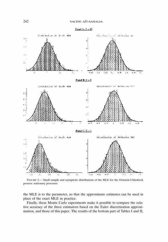
accurate are the various asymptotic distributions in Corollary 2? This questionis answered in Figures 2 and 3, where I plot the finite sample distributionsof the estimators (histograms) and the corresponding asymptotic distribution(solid line). The asymptotic distribution of �n − � reported in Panels A–C ofFigure 2 is from (5.1). Not surprisingly, as the drift parameter 5 makes the pro-cess closer and closer to a unit root (5 decreasing from 10 to 1), the quality ofthe asymptotic approximation (5.1) deteriorates and the small sample distributionstarts to resemble (5.3), which is strongly skewed. This only affects the driftparameter; the estimator of 2 behaves in small samples as predicted by theasymptotic distribution—which is compatible with the fact that the distributionfor estimating 2 is continuous when going through the 5= 0 boundary. Panel Aof Figure 3 reports results for the unit root case, with the asymptotic distributiongiven in (5.3). In the explosive case �5 < 0, Panel B of Figure 3 is based onthe Cauchy distribution (5.2), while Panel C exploits the possibility of randomnorming to obtain a Gaussian asymptotic distribution of the drift coefficient (see(A.69) in the Appendix). The diffusion estimator is identical in both Panels Band C, and is therefore not repeated in Panel C. Since the rate of convergencein nonstationary cases varies, both Panels B and C report the distribution of thedrift estimator scaled by the relevant rate of convergence, rather than the rawdistribution of 5n−5 as in all other panels. The simulations show that in bothnonstationary cases, and in the stationary case when sufficiently far away from aunit root, the asymptotic distribution of the drift estimator is an accurate guideto its small sample distribution.The second question these experiments address is: what is the dispersion of

the MLE around the true value? Tables I and II report the first four momentsof the finite sample and asymptotic distributions. For each of the parametervalues and the M samples, I also report in these tables the first two momentsof the differences between the true MLE estimators of 5 and 2, their Eulerversions and the estimators from using the method of this paper with one andtwo terms. This makes it possible, thirdly, to compare the MLE dispersion, orsampling noise, to the distance between the MLE and the various approximationsunder consideration. In particular, when selecting the order of approximation, itis unnecessary to select a value larger than what is required to make the distancebetween ��J n and �n an order of magnitude smaller than the distance between�n and the true value � (as measured by the exact MLE sampling distribution).These simulations show that the parameter estimates obtained with one and evenmore so two terms are several orders of magnitude closer to the exact MLE than


Figure 2.— Small sample and asymptotic distributions of the MLE for the Ornstein-Uhlenbeckprocess: stationary processes.

the MLE is to the parameter, so that the approximate estimates can be used inplace of the exact MLE in practice.Finally, these Monte Carlo experiments make it possible to compare the rela-

tive accuracy of the three estimators based on the Euler discretization approxi-mation, and those of this paper. The results of the bottom part of Tables I and II,


Figure 3.— Small sample and asymptotic distributions of the MLE for the Ornstein-Uhlenbeckprocess: nonstationary processes.

comparing the differences between the approximate and exact estimators, showthat the estimators with one and even more so with two terms are substantiallymore accurate than the Euler estimator, even though the latter is in an idealsituation in this example. Indeed, since the true transition function is Gaussian,the only approximation involved in the Euler estimation consists in using firstorder Taylor series expansions of the true conditional mean and variances rather


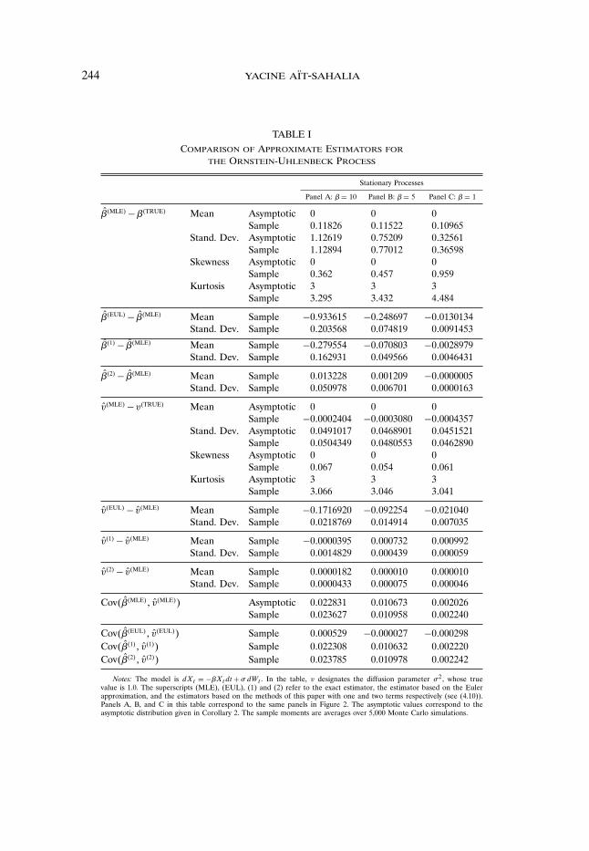
TABLE IComparison of Approximate Estimators for

the Ornstein-Uhlenbeck Process

Stationary Processes

Panel A: 5= 10 Panel B: 5= 5 Panel C: 5= 1

5�MLE−5�TRUE Mean Asymptotic 0 0 0Sample 0�11826 0�11522 0�10965

Stand. Dev. Asymptotic 1�12619 0�75209 0�32561Sample 1�12894 0�77012 0�36598

Skewness Asymptotic 0 0 0Sample 0�362 0�457 0�959

Kurtosis Asymptotic 3 3 3Sample 3�295 3�432 4�484

5�EUL− 5�MLE Mean Sample −0�933615 −0�248697 −0�0130134Stand. Dev. Sample 0�203568 0�074819 0�0091453

5�1− 5�MLE Mean Sample −0�279554 −0�070803 −0�0028979Stand. Dev. Sample 0�162931 0�049566 0�0046431

5�2− 5�MLE Mean Sample 0�013228 0�001209 −0�0000005Stand. Dev. Sample 0�050978 0�006701 0�0000163

v�MLE−v�TRUE Mean Asymptotic 0 0 0Sample −0�0002404 −0�0003080 −0�0004357




v�EUL− v�MLE Mean Sample −0�1716920 −0�092254 −0�021040Stand. Dev. Sample 0�0218769 0�014914 0�007035

v�1− v�MLE Mean Sample −0�0000395 0�000732 0�000992Stand. Dev. Sample 0�0014829 0�000439 0�000059

v�2− v�MLE Mean Sample 0�0000182 0�000010 0�000010Stand. Dev. Sample 0�0000433 0�000075 0�000046

Cov�5�MLE� v�MLE Asymptotic 0�022831 0�010673 0�002026Sample 0�023627 0�010958 0�002240

Cov�5�EUL� v�EUL Sample 0�000529 −0�000027 −0�000298Cov�5�1� v�1 Sample 0�022308 0�010632 0�002220Cov�5�2� v�2 Sample 0�023785 0�010978 0�002242

Notes: The model is dXt = −5Xtdt+ dWt . In the table, v designates the diffusion parameter 2, whose truevalue is 1.0. The superscripts (MLE), (EUL), (1) and (2) refer to the exact estimator, the estimator based on the Eulerapproximation, and the estimators based on the methods of this paper with one and two terms respectively (see (4.10)).Panels A, B, and C in this table correspond to the same panels in Figure 2. The asymptotic values correspond to theasymptotic distribution given in Corollary 2. The sample moments are averages over 5,000 Monte Carlo simulations.


TABLE IIComparison of Approximate Estimators for the Ornstein-Uhlenbeck Process

Non-Stationary Processes

Unit Root Explosive Root Explosive RootPanel A: 5= 0 Panel B: 5=−1 Panel C: 5=−1

5�MLE−5�TRUE Mean Asymptotic 0�09226 0 0Sample 0�09274 0�6026 0�0153

Stand. Dev. Asymptotic 0�16701 + 1Sample 0�16494 70�0266 1�0239

Skewness Asymptotic 2�265 undefined 0Sample 2�154 27�685 0�0428

Kurtosis Asymptotic 11�582 undefined 3Sample 9�527 1588�61 3�002

5�EUL− 5�MLE Mean Sample −0�00034314Stand. Dev. Sample 0�001004

5�1− 5�MLE Mean Sample 0�0000179Stand. Dev. Sample 0�0003434

5�2− 5�MLE Mean Sample −0�000000039Stand. Dev. Sample 0�000000313

v�MLE−v�TRUE Mean Asymptotic 0 0 0Sample 0�0002837 −0�001027 −0�001027




v�EUL− v�MLE Mean Sample −0�001782Stand. Dev. Sample 0�003171

v�1− v�MLE Mean Sample 0�000103Stand. Dev. Sample 0�000045

v�2− v�MLE Mean Sample 0�000011Stand. Dev. Sample 0�000044

Cov�5�MLE� v�MLE Asymptotic 0 0 0Sample 0�0003960 −1�0910−10 −1�0910−10

Cov�5�EUL� v�EUL Sample −0�0001255Cov�5�1� v�1 Sample 0�0003955Cov�5�2� v�2 Sample 0�0003953

Notes: The same notes as in Table I apply. In the explosive case, the dispersion of the simulated data around the meanof the process (zero) makes it impractical to simulate the approximate estimators. The panels match those of Figure 3. Thediffusion estimators in Panels B and C are identical.


TABLE IIIComparison of Approximate Estimators for the Vasicek,

Cox-Ingersoll-Ross, and Black-Scholes Models

Vasicek Cox-Ingersoll-Ross Black-ScholesdXt = 5�0−Xtdt dXt = 5�0−Xtdt dXt = 5Xt dt

+ dWt +X�5t dWt +Xt dWt

5�MLE−5�TRUE Mean 0�099674 0�09711 −0�0002561Stand. Dev. 0�178366 0�18772 0�0468815

5�EUL− 5�MLE Mean −0�015993 −0�00164 0�0017667Stand. Dev. 0�009873 0�03250 0�0008121

5�1− 5�MLE Mean −0�003675 0�00053 −0�0020946Stand. Dev. 0�005003 0�00105 0�0017052

5�2− 5�MLE Mean −0�000012 −0�00036 0�0000197Stand. Dev. 0�000270 0�00494 0�0000294

0�MLE−0�TRUE Mean 0�000023341 0�0006947 not applicableStand. Dev. 0�009078321 0�0011893 not applicable

0�EUL− 0�MLE Mean −0�000000003 0�0000089 not applicableStand. Dev. 0�000000071 0�0001789 not applicable

0�1− 0�MLE Mean 0�000001102 0�0001747 not applicableStand. Dev. 0�000109126 0�0002057 not applicable

0�2− 0�MLE Mean −0�000000017 −0�0000009 not applicableStand. Dev. 0�000003544 0�0001322 not applicable

�MLE−�TRUE Mean 0�00008690 0�000560 −0�00000165Stand. Dev. 0�00101568 0�004905 0�00966928

�EUL− �MLE Mean −0�00073620 −0�002768 0�00562312Stand. Dev. 0�00022012 0�001492 0�00189766

�1− �MLE Mean −0�00000043 0�000029 0�00005585Stand. Dev. 0�00000248 0�000391 0�00006205

�2− �MLE Mean −0�00000002 0�000013 −0�00000058Stand. Dev. 0�00000029 0�000387 0�00000117

Cov�5�MLE� �MLE 0�0000308 0�000202 0�00003267Cov�5�EUL� �EUL −0�0000077 −0�000017 0�00227254Cov�5�1� �1 0�0000305 0�000199 0�00003588Cov�5�2� �2 0�0000308 0�000200 0�00003262

Cov�5�MLE� 0�MLE 0�0000368 −0�00102 not applicableCov�5�EUL� 0�EUL 0�0000345 −0�00099 not applicableCov�5�1� 0�1 0�0000371 −0�00102 not applicableCov�5�2� 0�2 0�0000367 −0�00102 not applicable

Cov�0�MLE� �MLE 0�0000003112 0�0000006 not applicableCov�0�EUL� �EUL 0�0000002616 0�0000057 not applicableCov�0�1� �1 0�0000003134 0�0000006 not applicableCov�0�2� �2 0�0000003112 0�0000006 not applicable

Notes: The true values of the parameters, chosen to be realistic for US interest rates (Vasicek and CIR) and stockprices (Black-Scholes) respectively, are: 5= 0�5�0= 0�06� = 0�03 (Vasicek), 5= 0�5�0= 0�06� = 0�15 (CIR), and5= 0�2� = 0�3 (Black-Scholes). All moments reported are averages over 5,000 Monte Carlo replications.


than the exact expressions. By contrast, the approximate estimators correspond-ing to one and two terms mimic the moments of the MLE finite sample distribu-tion extremely closely, often to multiple accurate decimal places. Further MonteCarlo experiments for three standard models in finance (Black-Scholes (1973),Vasicek (1977), Cox-Ingersoll-Ross (1985)) reported in Table III reveal that theestimators proposed here outperform by orders of magnitude the Euler estima-tor, especially in non-Gaussian situations.

6� conclusions

This paper has constructed a series of explicit functions, based on Hermiteexpansions and converging to the conditional density of the diffusion process,under mild regularity conditions. This method makes maximum-likelihood a prac-tical option for the estimation of parameters in discretely-sampled diffusion mod-els. Beyond maximum-likelihood, the formulae for the expansion of pX applyto any specification of ��2, including nonparametric ones. Different types ofevidence have been provided in favor of this method. First, it largely outper-forms discrete approximations, binomial trees, PDE methods, and simulation-based methods in a direct comparison of speed and accuracy (Figure 1). Second,Monte Carlo experiments show that maximizing the log-likelihood approxima-tion provides parameter estimates that are very close to the true MLE (TablesI, II, and III) and outperforms by several orders of magnitude the alternativemethods—not only in terms of computational speed and ease of implementationbut also in terms of accuracy.Extensions to multi-dimensional diffusions (including unobservable state vari-

ables to be integrated out of the likelihood function, such as stochastic volatility)and applications to derivative pricing will be considered in future work. A furtherappeal of this method lies in its potential to be generalized to yet other typesof Markov processes, such as those driven by non-Brownian Lévy processes forinstance. As I remarked earlier, this generalization would involve different scalingX→ Y → Z, a non-Gaussian leading term for pZ (in this case a natural choiceis the limiting transition density of the driving process), and orthogonal functionsthat correspond to this leading term. But the basic principle remains valid: firstform an orthogonal series to approximate the density and prove its convergence;then determine its coefficients using repeated iterations of the infinitesimal gen-erator of the Markov process under consideration.

Department of Economics, Princeton University, Princeton, NJ 08544-1021,U.S.A., and NBER; [email protected]; http://www.princeton.edu/∼yacine

Manuscript received December, 1997; final revision received October, 2000.

APPENDIX: Proofs

Proof of Proposition 1: I treat the case where DY = �0�+, the other boundary configura-tions being dealt with similarly. Let sY �v��≡ exp�−

∫ v 2�Y �u��du� be the scale density of Y and


SY �y�� ≡∫ ysY �v� �dv its scale function.20 In each case, the lower limit of integration is a fixed

value in DY , the choice of which is irrelevant in what follows (i.e., for the purpose of determiningwhether or not the relevant quantities below are infinite or not). Let mY �v�� ≡ 1/sY �v�� be thespeed density of Y .

Step 1—Existence and unicity in law of a weak solution: This follows from the Engelbert-Schmidtcriterion (see, e.g., Theorem 5.5.15 in Karatzas and Shreve (1991), replacing � by DY throughout).To apply this result, note that continuity of �Y (and of course Y = 1) implies the local integrabilityrequirements for ��Y �/ 2Y and 1/ 2Y . Explosions are ruled out in Step 2 of this proof.

Step 2—Unattainability of the boundaries 0 and +: DefineQ ≡

∫ +

y

{∫ v

ymY �u��du

}sY �v��dv =

∫ +

y

{∫ +

usY �v��dv

}mY �u��du�

Q0 ≡∫ y

0

{∫ y

vmY �u��du

}sY �v��dv =

∫ y

0

{∫ u

0sY �v��dv

}mY �u��du�

(A.1)

From Feller’s test for explosions, Prob�TY = = 1 if and only if Q = and Q0 = (see, e.g.,Karatzas and Shreve (1991, Theorem 5.5.29) or Karlin and Taylor (1981, Section 15.6)). Near y=+,Assumption 3.1 gives the upper bound �Y �y��≤Ky for all y ≥E (without restraining how negative�Y can get); thus

Q =∫ +

y

{∫ +

usY �v��dv

}s−1Y �u��du=

∫ +

y

∫ +

ue−

∫ vu 2�Y �w��dw dvdu(A.2)

≥∫ +

y

∫ +

ue−

∫ vu 2Kwdwdvdu=

∫ +

y

{∫ +

ue−Kv

2dv

}eKu

2du�

Now by integration by parts∫ +

ue−Kv

2dv =

∫ +

uv−1ve−Kv

2dv = �2Ku−1e−Ku

2 − �2K−1∫ +

uv−2e−Kv

2dv

and, since∫ +u

v−2e−Kv2dv < u−2 ∫ +

ue−Kv

2dv, it follows that

(1+ �2K−1u−2) ∫ +

ue−Kv

2dv > �2Ku−1e−Ku

2� or∫ +

ue−Kv

2dv >

(2Ku+u−1)−1e−Ku2 �

Therefore

Q ≥∫ +

y

{∫ +

ue−Kv

2dv

}eKu

2du≥

∫ +

y�2Ku+u−1−1e−Ku

2eKu

2du=+�(A.3)

If y = 0, there exist constants .0�/�0 such that for all 0< y ≤ .0 and � ∈��Y �y�� ≥ /y−0 whereeither 0 > 1 and / > 0, or 0= 1 and k ≥ 1. If 0 > 1, we have for 0< v ≤ .0

sY �v��= exp{∫

v2�Y �w��dw

}≥ exp

{∫v2/w−0dw

}= /0 exp

{2/�0−1v−�0−1}(A.4)

and hence∫ u0 sY �v��dv =+. If however 0= 1,

sY �v��≥ exp{∫

v2/w−1dw

}= k0exp�−2/ ln�v�= k0v

−2/(A.5)

20 The scale function has the following intuitive interpretation: with x < a < x0 < b < x, the proba-bility that X will reach a before b (resp. b before a) starting from x0 is

(S�b��−S�x0� �/�S�b��−

S�a��)(resp. one minus this number). Taking the limit b→ x− and a→ x+ respectively, we see that

under Assumption 2.2 the probability that X will reach either boundary of DX in finite time is zero.


and∫ u0 sY �v��dv ≥

∫ u0 k0v

−2/ dv =+ again since we have assumed that /≥ 1 when 0= 1 (in fact,/ ≥ 1/2 would be enough to obtain an entrance boundary, but we have also required that / ≥ 1to insure that limy→0+ -Y �y�� < + since -Y �y�� = /�1−/y−2 if �Y �y�� = /y−1). In all theseinequalities, k0 denotes a different positive and finite constant. It follows from

∫ u0 sY �v��dv = +

and the finiteness of the measure mY in the second equality defining Q0 that Q0 =, i.e., y = 0 toois unattainable.

Step 3—Boundary classification for y = +∗: The boundary + is a natural boundary whenQ = N = , and an entrance boundary when Q = and N < (see, e.g., Karlin and Taylor(1981, Table 6.2)), where

N ≡∫ +

y

{∫ v

ysY �u��du

}mY �v��dv =

∫ +

y

{∫ +

umY �v��dv

}sY �u��du�(A.6)

Under Assumption 3, consider first the case where there exists E > 0 such that −Ky ≤�Y �y��≤Kyfor all y ≥ E. We then have

N =∫ +

y

{∫ +

umY �v��dv

}m−1

Y �u��du=∫ +

y

∫ +

ue∫ vu 2�Y �w��dw dvdu(A.7)

≥∫ +

y

∫ +

ue−

∫ vu 2Kwdw dvdu=

∫ +

y

{∫ +

ue−Kv

2dv

}eKu

2du=+

as in (A.3). If instead we have �Y �y��≤−Ky5� 5 > 1, for all y ≥ E, then

N =∫ +

y

∫ +

ue∫ vu 2�Y �w��dw dvdu≤

∫ +

y

∫ +

ue−

∫ vu 2Kw

5dw dvdu(A.8)

=∫ +

y

{∫ +

ue−Sv

5+1dv

}eSu

5+1du

where S ≡ 2�5+1−1K. By integration by parts∫ +

ue−Sv

5+1dv =

∫ +

uv−5v5e−Sv

5+1dv

= �S�5+1−1u−5e−Su5+1 − S−1�5+1−2

∫ +

uv−5−1e−Sv

5+1dv�

hence∫ +u

e−Sv5+1

dv < �2K−1u−5e−Su5+1 . So

N ≤∫ +

y

{∫ +

ue−Sv

5+1dv

}eSu

5+1du < �2K−1

∫ +

yu−5e−Su

5+1eSu

5+1du <+�(A.9)

Step 4—Boundary classification for y = 0: Among unattainable boundaries (i.e., given that Q0 =), whether 0 is an entrance or a natural boundary depends upon whether N0 < or N0 = respectively, where

N0 ≡∫ y

0

{∫ y

vsY �u��du

}mY �v��dv =

∫ y

0

{∫ u

0mY �v��dv

}sY �u��du�(A.10)

We have in all cases �Y �w��≥ /w−1 for some / > 0 (since if 0 > 1��Y �w��≥ /w−0 > /w−1; notethat this constant / is not necessarily ≥ 1/2). Then we can bound N0 as follows:

N0 =∫ y

0

∫ u

0exp

{∫ v

u2�Y �w��dw

}dvdu=

∫ y

0

∫ u

0exp

{−∫ u

v2�Y �w��dw

}dvdu(A.11)

≤∫ y

0

∫ u

0e−

∫uv 2//wdw dvdu=

∫ y

0

{∫ u

0v2/ dv

}u−2/ du= �2/+1−1

∫ y

0

{u2/+1

}u−2/ du

= �2/+1−1y2/2 <+�Therefore y = 0 is an entrance boundary for all 0≥ 1.


Proof of Proposition 2: Step 1—Existence of the transition density pY : Consider first thecase where DY = �−�+. The fact that Girsanov’s Theorem can be applied to Y follows fromKaratzas and Shreve (1991, 5.5.38); note that the explosion time of Y �TY , is infinity with probability1 as was proved in Proposition 1. By Girsanov’s formula, for every A in the usual -field,

Prob(Y� ∈A �Y0 = y0� �

)= E'M� ·1�W� ∈A�W0 = y0((A.12)

where 1�· denotes the indicator function and the nonnegative supermartingale

M� ≡ exp{∫ �

0�Y �WJ��dWJ −

12

∫ �

0�2Y �WJ��dJ

}(A.13)

is in fact a martingale for all �> 0. Setting TY ��y�y0� �≡E'M��W� = y�W0 = y0(, (A.12) becomes

Prob�Y� ∈A �Y0 = y0� �=∫ +

−1�y ∈ATY ��y �y0� �pBM��y �y0dy(A.14)

where pBM��y �y0 = �26�−1/2 exp{− �y− y02/�2�}. The existence of the transition density pY

follows from (A.14), and is given by pY ��y �y0� � = TY ��y �y0� �pBM��y �y0. Integration byparts inside the conditional expectation defining TY and the scaling property of Brownian motionallows TY to be further simplified (see Gihman and Skorohod (1972, Chapter 3.13), Dacunha-Castelleand Florens-Zmirou (1986), or Rogers (1985)) so that

pY ��y �y0� �= �26�−1/2e−�y−y02/2�+∫ yy0 �Y �w��dwE

[e�

∫ 10 -Y

(�1−uy0+uy+�1/2Bu��

)du

](A.15)

where �Bu/u ∈ '0�1(� designates a Brownian Bridge with B0 = B1 = 0.Step 2—Bound for pY : The strict positivity of pY (lower bound) follows from (A.15). From

Assumption 3, we obtain∫ yy0�Y �w��dw ≤H +L�y−y0��1+�y0�+Q�y−y02 for all �y� y0 in D2

Y ,where H�L, and Q are positive constants (if y ≥ 0, decompose the integral from y0 to E0, where�Y is bounded as a continuous function on a compact interval, and then from E0 to y, where �Yis bounded by Ky; a similar argument holds for y ≤ 0). Hence in general Q = K. This is an upperbound for the integral itself, not its absolute value. Then by the continuity of -Y �w�� in w, and itslimit behavior near the boundaries under Assumption 3, it follows that there exists ) ≥ 0 such that-Y �w��≤ ) for all w> 0 and � ∈� (in general, however, -Y will not be bounded below). Therefore

E

[exp

{�∫ 10-Y

(�1−uy0+uy+�1/2Bu��

)du

}]≤ e)��(A.16)

Collecting all terms we have that

pY ��y�y0� �≤ �26�−1/2e−�y−y02/2�+H+L�y−y0 ��1+�y0 �+K�y−y02 ×e)�(A.17)

≤ C0�−1/2e−3�y−y0

2/8�×eC1 �y−y0 � �y0 �+C2 �y−y0 �+C3 �y0 �+C4y20

provided that −1/�2�+Q ≤ −3/�8�, i.e., that 0 < � ≤ � ≡ �8Q−1. It is clear from the argumentthat we could replace 3/�8� in the bound for pY by any number less than but arbitrarily close to1/�2�, at the cost of reducing �, but this will not be necessary. Further, when �Y ≤ 0 near + and�Y ≥ 0 near −, Q can be set to 0 in the bound for

∫ yy0�Y �w��dw and hence � = + (in which

case we could also replace 3/�8� by 1/�2�).Step 3—Differentiability of pY : Suppose for now that we are allowed to differentiate under the

expectation sign in (A.15). It follows from the assumed smoothness of � and (hence �Y and -Y )


that

,pY ��y �y0� �,y

= �26�−1/2e�y−y022� +∫ yy0 �Y �w��dw(A.18)

×{{

− �y−y0�

+�Y �y��}E

[e�

∫ 10 -Y

(�1−uy0+uy+�1/2Bu��

)du

]+E

[�∫ 10u-′

Y

(�1−uy0+uy+�1/2Bu��

)du

×e�∫ 10 -Y

(�1−uy0+uy+�1/2Bu��

)du

]}where -′

Y �w�� ≡ ,-Y �w��/,w. The functions under the expectations depend continuously on yand I will now show that they are bounded by variables having constant expectation themselves.By uniform convergence, differentiating under the expectation will then have been legitimate andresult in a continuous derivative. First, we have � − �y− y0/�+�Y �y�� ≤ Q1��y�� y0� where Q1

is a polynomial of degree one in ��y�� y0�, with coefficients uniformly bounded in � ∈ �. Second∣∣E[AeB]∣∣≤ E[�A�eB] combined with (A.16) imply∣∣∣∣E[� ∫ 10 u-′

Y

(�1−uy0+uy+�1/2Bu��

)du×e�

∫ 10 -Y

(�1−uy0+uy+�1/2Bu��

)du

]∣∣∣∣(A.19)

≤ �E

[∫ 10u

∣∣∣∣-′Y

(�1−uy0+uy+�1/2Bu��

)∣∣∣∣du]e)��To bound the expected value on the right-hand side, recall that -′

Y �w�� has at most polynomialgrowth, thus in particular at most exponential growth. Hence there exists - > 0 and G> 0 such that�-′

Y �w�� ≤Ge-�w� and thus

E

[∫ 10u∣∣-′

Y

(�1−uy0+uy+�1/2Bu��

)∣∣du](A.20)

≤GE

[∫ 10ue��1−uy0+uy+�

1/2Bu � du]

=G∫ 10uE

[e��1−uy0+uy+�

1/2Bu �]du≤G∫ 10ue��1−uy0 �+�uy�E

[e�1/2 �Bu �]du�

Bu is distributed as N�0�u�1−u. If N is distributed as N�0� 2, the density of �N � is given by2�26−1/2−1 exp�−x2/2 2��x ≥ 0. Therefore for any constant a:

E'ea�N �(= 2�26−1/2−1∫ +

0eaxe−x

2/22dx = 2�26−1/2−1ea22/2

∫ +

0e−�x−a

22/22dx(A.21)

= ea22/2�26−1/2−1

∫ +

−e−�x−a

22/22dx = ea22/2

and it follows that E'e�1/2 �Bu �(= e�u�1−u/2. Hence

E

[∫ 10u∣∣-′

Y

(�1−uy0+uy+�1/2Bu��

)∣∣du]≤G∫ 10ue�1−u�y0 �+u�y�+�u�1−u/2 du≤Ge�y0 �+�y�(A.22)

(since u runs from 0 to 1) and we obtain (2.5) for all 0 < � < �, where the constant D0 is uniformin � and P is a polynomial of finite degree with coefficients also uniform in �.

Step 4—Consider finally (briefly) the case where DY = �0�+. What is required in the proof ofTheorem 1 is to show that the integral

∫ew2/2�,pZ��w�y0� �/,w�2dw converges. That is, after a

change of variable Z→ Y , we need to show that the integral∫ +

0�1/2e�y−y0

2/2��,pY ��y�y0� �/,y�2 dy


converges at both boundaries 0+ and +. The boundary 0+ is either an entrance or a naturalboundary for Y , and in both cases limy→0+ ,pY ��y�y0� �/,y = 0 (see McKean (1956, Remark 4.2,page 541). Hence the integral converges at the left boundary 0. The change of measure in Step 1above is no longer applicable in its simplest form, because the distribution of Y and that of aBrownian motion are no longer absolutely continuous with respect to one another since Y is nowdistributed on a subset of the real line whereas a Brownian motion is distributed on the entire realline. However, we can still transform Y into a Brownian motion, but the Radon-Nikodym derivativeis only a local martingale instead of a martingale. Girsanov’s Theorem now gives for y > 0� y0 > 0:

pY ��y �y0� �= pBM��y �y0e∫ yy0�Y �w��dwE

[e∫�0 -Y �Wu��du

∣∣W� = y�W0 = y0�� < T0]

(A.23)

where inside the expectation W follows the law of a Brownian motion and T0 indicates the first timeW hits 0. From (A.23), the same bounds can be derived.

Proof of Corollary 1: The existence and unicity in law of a solution of (1.1) follows, as inProposition 1, from an application of Theorem 5.5.15 in Karatzas and Shreve (1991) replacing � byDX throughout. Note that �x�� > 0 for every x in DX and � in �; hence the nondegeneracy con-dition of the theorem is fulfilled (the only possible local degeneracy of , if any, occurs as x→ 0+,but 0 �∈DX). The continuity of � and implies the local integrability requirements for ��/ 2 and1/ 2. Explosions are ruled out by showing that Prob�TX == 1. This in turn follows from the factthat Yt = )�Xt� �. The fact that )�x�� tends to one of the boundaries of DY when x tends to oneof the boundaries of DX means that X would not be able to reach one of its boundaries withoutY also doing so. But we already know that Y cannot do it (recall Proposition 1). Hence X cannotexplode. Finally, the existence of pX and its derivatives follows from the Jacobian formula; specifi-cally pX��x �x0� � = �x��−1pY ��)�x�� )�x0� �� and the differentiability of pY proved inProposition 2 (and of course the differentiability of and ) which results from Assumption 2) extendto pX .

Proof of Theorem 1: Step 1—Let � > 0 be the constant defined in Proposition 2 (possibly�=). Let AX be a compact set contained in DX , and consider x0 in AX . Let AY be the compactset that contains the values of )�x0� � as x0 varies in AX and � in the closure of � (recall that � isbounded). Define S��x�x0� �≡ �−1/2�)�x��−)�x0� �. We seek to bound:

�pX��x�x0� �−p�JX ��x�x0� �� = �x��−1�−1/2�pZ��S��x�x0� ��)�x0� �� (A.24)

−p�JZ �� S��x�x0� ��)�x0� �� For that purpose, we will bound the jth coefficient in the approximating function p�JZ . The =

�JZ ’s

in (2.12) are well-defined since by (2.4), the moments uY ��y0� �� j ≡∫ +− �y�jpY ��y�y0� �dy are

finite for all j ≥ 0 as a result of

uY ��y0� �� j≤ e�C3 �y0 �+C4y20 �C0�1/2

∫ +

−�w−y0�j e�−3w2/8�+C1 �y0 � �w�+C2 �w�� dw(A.25)

where the variable y has been changed to w= y−y0. For each � and y0 there exists a value y��y0≥0 such that for all w� �w� ≥ y��y0 implies that −3w2/8�+C1�y0� �w � +C2�w� ≤ −5w2/16�.Next, integration by parts with �j+1Hj�z=−dHj+1�z/dz yields

=�jZ ��y0� �= �j!−1

∫ +

−Hj�wpZ��w�y0� �dw(A.26)

=− �j!−1�j+1−1∫ +

−H ′

j+1�wpZ��w �y0� �dw

=− ��j+1!−1Hj+1�wpZ��w�y0 � �]+

−

+ ��j+1!−1∫ +

−Hj+1�w�,pZ��w�y0 � �/,w�dw�


With y = y0+�1/2w and (2.4), we have that0< pZ��w�y0� �≤ a0 exp�−3w2/8�exp�a1�w��y0�+a2�w�+a3�y0�+a4y20�(A.27)

where the constants ai� i= 0� � � � �4, are uniform in � ∈�. By Theorem II in Stone (1928), there existsa constant K such that for all z in R and every integer j , �Hj�z� ≤K�j!1/2j−1/4�1+2−5/4�z5/2��ez2/4.Therefore ∣∣��j+1!−1Hj+1�wpZ��w �y0� �

∣∣(A.28)

≤ ��j+1!−1/2�j+1−1/4K�1+�w5/2/25/4��ew2/4a0e−3w2/8ea1 �w� �y0 �+a2 �w�+a3 �y0 �+a4y20

and hence ��j+1!−1Hj+1�wpZ��w�y0� �]+− = 0.

Step 2—Proof that the expansion p�JZ of pZ converges: Define

Wj��y0� �≡ �j!−1∫ +

−Hj�w�,pZ��w�y0� �/,w�dw�(A.29)

We can bound the terms of order j ≥ 1 in the series for pZ according to

�=�jZ ��y0� �Hj�z� = ��j+1!−1∣∣∣∣ ∫ +

−Hj+1�w�,pZ��w �y0� �/,w�dw

∣∣∣∣�Hj�z�(A.30)

= �Wj+1��y0� ��Hj�z�≤K

{1+ ∣∣z5/2/25/4∣∣}ez2/4×�j−1/4�j!1/2�Wj+1��y0� ��

≤K�1+�z5/2/25/4��ez2/4×�j−1/4�j+1−1/2��j+1!1/2�Wj+1��y0� ��≤K�1+�z5/2/25/4��ez2/4�j−1/2�j+1−1+ �j+1!W2j+1��y0� ��/2

since �05� ≤ �02 +52/2. The first series on the right-hand side, ∑ j−1/2�j + 1−1, is convergent. Itremains to prove that the series

∑j=0 j!W2j ��y0� � converges. The integral

∫ +− e

w2/2�,pZ��w �y0� �/,w�2dw converges, since from (2.5) one can conclude that:

�,pZ��w �y0� �/,w� ≤ b0e−3w2/8R��w�� y0�eb1 �w��y0 �+b2 �w�+b3 �y0 �+b4y20(A.31)

where R is a polynomial of finite order in ��w�� y0� with coefficients uniform in � ∈ �, and wherethe constants bi� i = 0� � � � �4, are uniform in � ∈�.Then expand the squared term in

0 ≤∫ +

−ew2/2

{,pZ��w�y0� �/,w−<�w

J∑j=0Wj��y0� �Hj�w

}2dw

=∫ +

−ew2/2�,pZ��w �y0� �/,w�2 dw

−2�26−1/2J∑j=0Wj��y0� �

∫ +

−�,pZ��w �y0� �/,w�HJ �wdw

+�26−1J∑j=0

J∑k=0Wj��y0� �Wk��y0� �

∫ +

−e−w

2/2Hj�wHk�wdw

=∫ +

−ew2/2�,pZ��w �y0� �/,w�2 dw− �26−1/2

J∑j=0j!W2j ��y0� �

and the (dominated) convergence of the series on the right-hand side follows. Further, the seriesconverges uniformly with respect to � in � and to y0 in the compact set AY .


Hence p�JZ ��z �y0� �=<�z∑J

j=0 =�jZ ��y0� �Hj�z is convergent as J →. Note that the con-

vergence is uniform in z over the entire real line since the two series in (A.30) are independent of zand hence converge uniformly with respect to z. The convergence is also uniform with respect to �in � and y0 in the compact set AY .

Step 3—Proof that the limit of p�JZ ��z �y0� � (which we now know exists) is indeed

pZ��z �y0� �: Let qZ��z �y0� � ≡ limJ→ p�JZ ��z �y0� �. qZ is continuous in z as the uniform

limit of a series of continuous functions. Further, with .j+1 ≡ j−1/2�j + 1−1 + �j + 1!W2j+1��y0� �,note that there exists a constant K0 such that

<�z∣∣=�jZ ��y0� �Hj�z

∣∣≤K�1+ ∣∣z5/2/25/4∣∣�e−z2/4.j+1 ≤K0e−3z2/8.j+1(A.32)

(for z large enough) and hence qZ satisfies the same bound as pZ (which itself follows from that ofpY in Proposition 2). Therefore the integral �k!−1

∫ +− qZ��w �y0� �Hk�wdw exists and

�k!−1∫ +

−p�JZ ��w �y0� �Hk�wdw(A.33)

= �k!−1J∑j=0=�jZ ��y0� �

∫ +

−�26−1/2e−w

2/2Hj�wHk�wdw

={=�kZ ��y0� � if k ≤ J

0 if k > J

because∫ +− �26

−1/2e−w2/2Hj�wHk�wdw = j! if k = j , and 0 otherwise (see, e.g., Sansone (1991,

page 308)). Hence it follows that �k!−1 ∫ +− qZ��w�y0� �Hk�wdw = =k��y0� �, and so pZ and

qZ have the same =k coefficients for all k ≥ 0. To finish, consider two continuous functions satisfyingthe same first bound as in Proposition 2 and sharing the same =k coefficients for all k: they mustbe equal. Indeed, define the difference rZ��w�y0; �≡ qZ��w�y0� �−pZ��w�y0� �. The integralof rZ against polynomials wk of all orders k ≥ 0 is equal to zero (since any polynomial of order kis a linear combination of the first k polynomials Hk) and therefore by Weierstrass’s approximationtheorem the function rZ is identically zero.

Step 4—Back to pX : I have shown that, for every . > 0, there exists J.�AY �� such that forall J ≥ J.�AY ��, the bound

∣∣pZ��z�y0� �−p�JZ ��z�y0� �∣∣ ≤ . holds for all z ∈ R�y0 ∈AY , and

� ∈�. If is globally nondegenerate under Assumption 2(1), −1�x�� < c−1 <+ implies that forall J ≥ J.�AX��

∣∣pX��x�x0� �−p�JX ��x�x0� �∣∣≤ . for all x in R, x0 ∈AX and � ∈�. If not, for

every . > 0, there exists a constant c. such that −1�x�� < c−1. <+ for all x ∈ '.�+ and � ∈�.Therefore the uniform convergence of p�JZ to pZ for z in R implies the uniform convergence of p

�JX

to pX for x in '.�+� since for such x’s equation (A.24) implies∣∣pX��x �x0� �−p�JX ��x �x0� �∣∣(A.34)

≤ c−1. �−1/2∣∣pZ��S��x�x0� ��)�x0� �� −p�JZ �� S��x�x0� ��)�x0� ��

∣∣�Proof of Proposition 3: First verify that (3.4) holds. By Taylor’s Theorem, we have

�n(�+ I−1/2n ��hn

)−�n��= hnI−1/2n ��n��+hTn I−1/2n ��n

˜��I−1/2n ��hn/2(A.35)

for every bounded sequence hn such that �+ I−1/2n ��hn ∈ �, with �n between � and �+ I−1/2n ��hn.Now under Assumption 4, we have, again by Taylor’s Theorem,∥∥I−1/2n ��n��I

−1/2n ��−Gn��

∥∥≤ ∥∥I−1/2n ��...� n�

˜�I−1/2n ��∥∥×∥∥I−1/2n ��

∥∥(A.36)

where the first term on the right-hand side is bounded in probability as the norm of Rn��˜�, while

the second term, which arises because both � and ˜� are in the same I 1/2n ��-neighborhood, goes tozero, so

�n(�+ I−1/2n ��hn

)−�n��= hnSn��−hTnGn��hn/2+op�1�(A.37)


Therefore under (3.5) we have the LAMN structure (see, e.g., Jeganathan (1995, Definition 3,page 837)), and under (3.10) the LABF structure (see, e.g., Jeganathan (1995, Definition 4,page 850)).By Taylor’s Theorem applied to the score function, �n��− �n�� = −�n��n− �, i.e., Sn�� =

I−1/2n ��Vn��= I−1/2n ��Hn��I−1/2n ��I 1/2n ��n−� so

I 1/2n ��n−�=[I−1/2n ��Hn��I

−1/2n ��

]−1Sn��(A.38)

and hence as in (A.36) we have

I 1/2n ��n−�−G−1n ��Sn��= op�1�(A.39)

Now both (3.6) and (3.11) follow from the joint convergence in distribution of �Sn�Gn underLAMN and LABF respectively, and the Continuous Mapping Theorem (e.g., Hall and Heyde (1980,Theorem A.3, page 276) applied to (A.39). The efficiency statement (3.8) under LAMN follows fromapplying Theorem 3 in Basawa and Scott (1983, Chapter 2.4, Theorem 3, page 60); the Normalasymptotic variance comparison follows from Chapter 2.3, Corollary 2, page 53.Under stationarity, the convergence in (3.5) follows from the Central Limit Theorem and the Law

of Large Numbers (see, e.g., Hall and Heyde (1980)), and the fact that E�

[n−1Hn��

] = n−1in�� =i��, so

Gn�� = I−1/2n ��Hn��I−1/2n ��= I−1/2��

[n−1Hn��

]I−1/2��(A.40)

p→ I−1/2��i��I−1/2��≡G��

G�� is a nonrandom positive definite matrix provided that i�� is (which is guaranteed by (3.2)),and we obtain the classical result (3.9) (see, e.g., Billingsley (1961)).I now show that the condition on Rn�� in Assumption 4 is automatically satisfied under sta-

tionarity. In (A.15), let

b��≡∫ y

y0

�Y �w��dw� fu��≡ �-Y(�1−uy0+uy+�1/2Bu��

)� c��≡

∫ 10fu��du�(A.41)

q��≡ ln(pY ��y �y0� �)=− ln�26�/2− �y−y02/2�+b��+ ln(E'ec��()�(A.42)

and recall that �Y and -Y , hence fu and c, are three times differentiable in � under Assumption 2.1.From (A.42), it follows that

q��= b��+ E'c��ec��(

E'ec��(� q��= b��+ E'�c��+ c��2ec��(

E'ec��(− E'c��ec��(2

E'ec��(2�(A.43)

...q��= ...b��+ E'�

...c ��+3c��c��+ c��3ec��(

E'ec��((A.44)

− 3E'�c��+ c��2ec��(E'c��ec��(

E'ec��(2+ 2E'c��e

c��(3

E'ec��(3�

where for simplicity I use the same notation as if the parameter vector were one-dimensional. Letv�� play the role of c�� c��+ c��2, and ...c ��+3c��c��+ c��3 respectively and apply Holder’sInequality, with p = 4/3 and r = 4, to

�E'v��ec��(� ≤ E'�v��ec��(= E'ec��/pec��/q �v��(≤ E'ec��(1/pE'ec��v��q(1/q �(A.45)

Under Assumption 3, the function v�� has at most polynomial growth in w and as a result itfollows from the same calculations as in (A.19)–(A.22), and the fact that c��≤ ) that

E'ec��v��q(1/q ≤Ge)+�y0 �+�y�(A.46)


(where G is a constant) for all the v�� listed above. We therefore have shown that�E'v��ec��(�/E'ec��(≤Ge)+�y0 �+�y�E'ec��(1/p−1 ≤Ge)+�y0 �+�y�E'ec��(−1/4. Recall next that �Y � �Y , and...�Y all have at most polynomial growth. Hence there exist a constant G and a finite order polynomial

P such that �q��≤P��y��y0�+Gea�)+�y�+�y0 ��E'ec��(−1/4�

�q��≤P��y��y0�+Gea�)+�y�+�y0 ��E'ec��(−1/4+E'ec��(−1/2��...q��≤P��y��y0�+Gea�)+�y�+�y0 ��E'ec��(−1/4+E'ec��(−1/2+E'ec��(−3/4�

(A.47)

From this it follows that

E[�q��∣∣Y0 = y0

]≤ ∫ y

y

{P��y�� y0�+Gea�)+�y�+�y0 �E'ec��(−1/4

}(A.48)

× �26�−1/2e−�y−y02/2�+b��E'ec��( dyis finite (the negative powers of E'ec��( get compensated), and similarly for E'�q��∣∣Y0 = y0( andE'�...q��∣∣Y0 = y0(. Hence E'�

...q��( is bounded, and by the Law of Large Numbers

Rn�� = I−1/2n ��Tn��I−1/2n ��

p−→ I−1/2��E[...q��

]I−1/2��(A.49)

which is a finite constant, uniformly bounded in �.By using the top inequality in (A.47) and squaring it, it also follows as in (A.48) that E'�q��2∣∣Y0 =

y0( is bounded (the highest negative power becomes �E'ec��(−1/42 and therefore in�� is finite.The fact that the derivatives of ln�pX are bounded follows from the bounds just given for the

derivatives of ln�pY , and the differentiation chain rule applied to (2.9). Under Assumption 2, 1/ isbounded (except possibly near a 0 boundary) and the function ) defined in (2.1) and its derivativeshave at most polynomial growth. The same bounds as in (A.48) (with negative powers E'ec��(−1/2

and E'ec��(−3/4 similarly annihilated by E'ec��( apply to the second and third derivatives of ln�pY with respect to y and y0 rather than �. Thus

, ln�pX,�

=−

+ , ln�pY ,�

+ )�x� � , ln�pY ,y

+ )�x0� �, ln�pY ,y0

(A.50)

(and the next two derivatives) are bounded similarly to (A.48) using the bounds for the derivativesof ln�pY in (A.50).

Proof of Theorem 2: Step 1—Fix . > 0 and x0 ∈ R. Let r�J X ��x�x0� � = pX��x�x0� �−p�JX ��x�x0� �,

R�JX ��x�x0��≡ sup

�∈�

∣∣r�J X ��x�x0� �∣∣(A.51)

and also define the corresponding quantities for Y and Z. By Theorem 1, the conver-gence of p�JY ��y�y0� � to pY ��y�y0� � is uniform in y over DY and in � over �, and iny0 over bounded subsets AY of Dy . Hence there exists J.��AY �� such that for all J ≥J.��AY ��M sup�∈� supy∈DY supy0∈AY �r�J Y ��y�y0� ��< .. Now recall:

�pX��x�x0� �−p�JX ��x�x0� �� = �x��−1∣∣pY ��)�x��)�x0� ��

−p�JY ��)�x��)�x0� �� ∣∣

and for given x0 let AY be the set of y0 described by )�x0� � as � varies in �. Since � is bounded and) is continuous in � ( is by Assumption 2.1), AY is bounded. It follows that for all J ≥ J.��AY ��

R�JX ��x�x0��≤ sup

�∈�

{�x��−1

}× sup�∈�

supy∈DY

supy0∈AY

∣∣r�J Y ��y�y0� �∣∣≤ sup

�∈�

{�x��−1

}×.�(A.52)


Let Q−1�x ≡ sup�∈��x��−1�, which is finite by the boundedness of � and the continuity of−1 in �. Then for m= 1 and m= 2, we have that∣∣∣∣E�0

[{R�JX ��Xt+��Xt��

}m∣∣Xt = x0

]∣∣∣∣≤ ∫ x

x

∣∣R�JX ��x�x0��

∣∣mpX��x�x0� �0dx(A.53)

≤ .m∫ x

xQ−m�xpX��x�x0� �0dx

i.e., limJ→E�0

[{R�JX ��Xt+��Xt��

}m∣∣Xt = x0] = 0 for m = 1�2� provided that we prove that the

two integrals∫ xxQ−m�xpX��x�x0� �0dx�m= 1�2� converge.

Step 2—Bounding the integral in the right-hand side of (A.53): A difficulty only arises when DX =�0�+� limx→0+ �x��= 0 (otherwise Q−m�x≤ c−m and then ∫ x

xQ−m�xpX��x�x0� �0dx ≤ c−m).

Applying the change of variable X→Y , I will prove convergence of the integral∫ yyQ−m�)−1�y� �×

pY ��y�y0� �dy �Q−1 means 1/Q whereas )−1 represents the inverse of the function )). We needto consider the two cases where y ≡ limx→0+ )�x�� is either 0+ or −. Under Assumption 2.1, wehave that −1�x�� ≤ $−1x−% for all 0< x ≤ #0 and � ∈�. For 0< x ≤ #0, we have

∫ x0 du/�u�� ≤∫ x

0 $−1u−% du = $−1�1−%−1x1−% if 0 ≤ % < 1, and therefore y = 0+ by taking the limit as x tends to

0+. Let x = )−1�y� �, and I have just shown that for y near 0+� y ≤ $−1�1−%−1x1−%, from which itfollows that )−1�y� �≥ �$�1−%y1/�1−% and consequently

Q−m�)−1�y� �≤ $−m')−1�y� �(−m% ≤ $−m�$�1−%y−m%/�1−%�(A.54)

So naturally the upper bound tends to + as y tends to 0+. The issue is whether this upper boundincreases faster than pY decreases as y tends to 0+. To answer this question, we need to call uponAssumption 3.1. For 0< y ≤ .0,

e∫ y.0

�Y �w��dw = e−∫ .0y �Y �w��dw ≤ e−/

∫ .0y w−0dw =

{.−/0 y

/ if 0= 1�e/�0−1.

−�0−10 −/�0−1y−�0−1 if 0 > 1�

(A.55)

will provide an upper bound to pY for y near 0+ (see the proof of Proposition 2; the other termsare bounded near 0+). It is clear that if 0 > 1 the left tail of pY decays exponentially fast, while theupper bound for

Q−m�)−1�y� �≤ $−m')−1�y� �(−m% ≤ $−m�$�1−%y−m%/�1−%(A.56)

increases only geometrically, so the integral will converge. If 0 = 1, then the tail of pY is boundedabove by y/ and therefore the integral will converge if /≥ 2%/�1−%. This is given by Assumption 5.If instead %≥ 1, then

y = limx→0+

∫ x

+−1�u��du=

∫ #0

+−1�u��du+ lim

x→0+

∫ x

#0

−1�u��du

where∫ #0+

−1�u��du≤ 0and

limx→0+

∫ x

#0

−1�u��du≤ limx→0+

∫ x

#0

$−1u−% du= limx→0+

{$−1 ln�x if %= 1�−$−1�%−1−1x−�%−1 if % > 1�

(A.57)

which is −, so y = − when % ≥ 1. In that case, we have for y near y M Q−m�)−1�y� � ≤$−m')−1�y� �(−m%. Let x = )−1�y� �. From the same calculation as above, we have y ≤ $−1 ln�x if%= 1. Thus )−1�y� � ≥ e$y and therefore Q−m�)−1�y� � ≤ $−me−m%$y . Now from (A.17), we knowthat pY is bounded above by a term of the form e−3y

2/8�, so the integral of e−m%$ye−3y2/8� converges fory near −. If %> 1� y≤−$−1�%−1−1x−�%−1 and therefore )−1�y� �≥ �−$�%−1y−1/�%−1, and thus


Q−m�)−1�y� � ≤ $−m�−$�%−1ym%/�%−1, which again tends to + as y tends to −, but not fastenough to overcome the decay e−3y2/8� of pY . Hence the integral

∫ yyQ−m�)−1�y� �pY ��y �y0� �dy

converges near y =− when %≥ 1. Therefore from (A.53) we conclude that

limJ→

E�0

[�R

�JX ��Xt+��Xt��

m �Xt = x0]= 0 for m= 1�2�(A.58)

Step 3—The convergence of its first two moments given by (A.58) to zero imply by Chebyshev’sInequality that the sequence R�J

X ��Xt+��Xt�� converges to zero in probability, given Xt = x0,that is:

limJ→

Prob(∣∣R�J

X ��Xt+��Xt��∣∣> .�Xt = x0� �0

)= 0�(A.59)

By Bayes’ Rule we have

Prob(∣∣R�J

X ��Xt+��Xt��∣∣> .��0)(A.60)

=∫ +

−Prob

(∣∣RJX��Xt+��Xt��

∣∣> .∣∣Xt = x0� �0)6t�x0� �0dx0

where 6t�x0� �0≡ ,Prob�Xt ≤ x0� �0/,x0 denotes the unconditional (or marginal) density of Xt atthe true parameter value. Note that since we are not assuming that the process is strictly station-ary, that density depends on t. Now since 0 ≤ Prob(∣∣R�J

X ��Xt+��Xt��∣∣ > .�Xt = x0� �0

) ≤ 1 and∫ +− 6t�x0� �0dx0 = 1 it follows from Lebesgue’s Dominated Convergence Theorem (see, e.g., Haaserand Sullivan (1991, Theorem 6.8.6)) that

limJ→

Prob(∣∣R�J

X ��Xt+��Xt��∣∣> .��0)= 0�(A.61)

Step 4—Convergence as J →: I have now established that

p�JX ��Xt+��Xt��

p−→ pX��Xt+��Xt�� as J →�

Before taking the logarithm of p�JX , we need to trim it to insure that it is positive on the entire supportDX . The roots of the Hermite polynomials are such that p

�JX > 0 on an interval '−cJ � cJ ( with cJ →

as J →. Let aJ be a positive sequence converging to 0 as J →. Define $J as a (smooth) versionof the trimming index taking value 1 if p�JX > aJ and aJ otherwise. As a consequence of the bound(2.4), pX is tight, i.e., for every . > 0 there always exists a compact space K. ⊂ DX that contains1−. of the mass of the density pX . As a result, trimming by $J is asymptotically irrelevant (as J →), that is $J

p−→ 1. It follows that $Jp�JX

p−→ pX and furthermore ln'$Jp�JX ��Xt+� �Xt��(

p−→ln'pX��Xt+��Xt��( by the continuity of the logarithm. Thus for any given n we have obtained that��J n ��

p−→ �n�� as J →, uniformly in �. The convergence of the respective argmax in ��J n

p−→ �nas J → is then an application of standard methods since ��J n �� and �n�� and their derivativesare both continuous in � for all n and J . This proves part (i) of the Theorem.

Step 5—Convergence as n→ . From Step 4, a value of Jn can be chosen for each n to make��Jnn − �n� arbitrarily small in probability. In particular, one can select Jn → such that ��Jnn − �n =op�I

−1/2n ��0 as n→. This proves part (ii) of the theorem.

Proof of Proposition 4:21 Under the assumptions made on �Y , the boundaries are entrance(see Proposition 1). The former insures stationarity of Y (see the discussion following Proposition1). It is also the case that the scale measure sY �v��≡ exp�−

∫ v 2�Y �u��du� diverges exponentiallyfast at each boundary. The spectrum of A�� is discrete, from Section 4.1 in Hansen, Scheinkman,

21 I am grateful to Ernst Schaumburg for providing a key element in this proof.


and Touzi (1998).22 That is, there exists a countable number of eigenvalues -p and eigenfunc-tions <p� p = 0�1� � � � , forming an orthonormal basis in L2�6Y such that for all functions f inthe domain of A��, A�� · f = ∑

p=0 -p�f �<p�<p where �·� ·� denotes the natural inner productof L2�6Y . Now polynomials f and their iterates (by repeated application of the generator) retaintheir polynomial growth characteristic near the boundaries; so they are all in L2�6Y and satisfylimy→y f

′�y/sY �y�� = limy→y f′�y/sY �y�� = 0. This follows from the exponential divergence of

sY �y� � near both boundaries whereas polynomials and their iterates diverge at most polynomially(recall that under Assumption 3 �Y and its derivatives have at most polynomial growth; multiply-ing and adding functions with polynomial growth yields a function still with polynomial growth).Using then the Hansen, Scheinkman, and Touzi (1998, page 10) characterization of the domain ofthe generator of a scalar diffusion, polynomials and their iterates are in the domain of the gen-erator. Since f is in L2�6Y , it follows that f = ∑

p=0⟨f �<p

⟩<p with

∑p=0

⟨f �<p

⟩2<. Moreover,

Ak�� · f =∑p=0 -

kp

⟨f �<p

⟩<p. Therefore:

K∑k=0Ak�� · fk!−1�k =

K∑k=0

(∑p=0-kp�f �<p�<p

)k!−1�k =

∑p=0

(K∑k=0-kpk!−1�k

)�f �<p�<p(A.62)

by Fubini’s Theorem. Y being a time-reversible diffusion, its eigenvalues -p are all real and negative.Therefore �∑K

k=0 -kpk!−1�k� ≤ 1, with limit exp�-p�≤ 1, and it follows that

∑p=0

(K∑k=0-kpk!−1�k

)2�f �<p�2 ≤

∑p=0

�f �<p�2 <(A.63)

for all J and by the dominated convergence theorem the series∑K

k=0Ak�� · fk!−1�k converges as

K→.

Proof of Corollary 2: Step 1—Part (i) follows directly from (3.9).Step 2—Part (ii): With the notation .i� ≡Xi�− e−5�X�i−1�, the matrices Hn�� In�� and G��

of Section 3 can be calculated explicitly. It is easy to see that the terms of Hn�� are of the form:

[Hn��

]11= a1��n+a2��

n∑i=1X2

�i−1�+a3��n∑i=1X�i−1�.i�+a4��

n∑i=1.2i��(A.64)

[Hn��

]22= b1��n+b2��

n∑i=1.2i��(A.65)

[Hn��

]12= c2��

n∑i=1X�i−1�.i�+c3��

n∑i=1.2i��(A.66)

where ak� bk, and ck are functions of the parameters �. Now E[∑n

i=1X2�i−1�

]and E

[∑ni=1 .

2i�

]are

asymptotically equivalent as n→ to e−2n5� 2/25�e−25�−1 and n 2�e−25�−1/25 respectively, andE[∑n

i=1X�i−1�.i�]= 0 (see White (1958) and Anderson (1959)). So to calculate an asymptotic equiv-

alent for In�� = diag�E�'Hn��(� we only need a2�� = 25�2e−25�/ 2�e−25�− 1, b1�� = −1/2 4�

22 Natural boundaries do not necessarily lead to a discrete spectrum (for example, in some instancesa mixed discrete-continuous spectrum results). A stationary Ornstein-Uhlenbeck process (i.e., onewith positive mean reversion) is an example of a process with natural boundaries and a discretespectrum. What Proposition 4 shows is that having a discrete spectrum is a sufficient condition forthe convergence of the series (4.3).


and b2�� = 5/2 6�e−25�−1 to obtain that 'In��(11 is equivalent to e−2�n+15��2/�e−25�−12 while'In��(22 = n/2 4. Finally,

Gn��=(

'Hn��(11/'In��(11 'Hn��(12/√'In��(11'In��(22

'Hn��(12/√'In��(11'In��(22 'Hn��(22/'In��(22

)p−→G��

=(P2'1( 00 1

)�

(A.67)

because �25�1− e−25�/ 2e−2n5��∑ni=1X

2�i−1�

p−→ P2'1( = N�0�12, while∑n

i=1 .2i� = Op�n

1/2 and∑ni=1X�i−1�.i� = Op�e

−n5�. Therefore (5.2) follows, which is a non-Gaussian distribution underdeterministic scaling by the asymptotic equivalent of

√'In��(11. Since

Prob('G−1/2(11×N�0�1≤z

)=Prob(N�0�1≤z'G1/2(11)=∫ +

0

∫ z√g

−

e−n2/2

√26

e−g/2√26g

dndg(A.68)

yields by differentiation with respect to z the density 1/6�1+z2� 'G−1/2(11×N�0�1 is the Cauchydistribution. Alternatively, we obtain a Gaussian distribution under random scaling by the asymptoticequivalent of

√'Hn��(11:√25�2

∑ni=1X

2�i−1�

2�e25�−1 �5n−5 d−→N�0�1�(A.69)

Step 3—Part (iii): 'In��0(11 is asymptotically equivalent to �−2E[∑n

i=1X2�i−1�

], i.e., to n2�2/2,

when 5= 0. Further,

'Sn��0(1 = 'In��0(−1/211

{2−1n�−−2

n∑i=1X�i−1�.i�−2−1−2

n∑i=1.2i�

}�(A.70)

'Gn��0(11 = 'In��0(−111

{6−1n�2+�−2

n∑i=1X2

�i−1�+�−2n∑i=1X�i−1�.i�+�3−1−2

n∑i=1.2i�

}�(A.71)

Thus('Sn��0(1� 'Gn��0(11

) d−→(2−1/2�1−W 2

1 �2∫ 10 W

2J dJ

)since from White (1958):

(∑ni=1X�i−1�.i�2n 2�

�

∑ni=1X

2�i−1�

n2 2�

)d−→(W 21 −1�

∫ 10W 2

J dJ

)�(A.72)

And (5.3) follows from (3.11) with MJ =WJ and 2∫ 10 WJ dWJ =

∫ 10 dW

2J −

∫ 10 dJ =W 2

1 − 1. In thiscase the convergence Gn →G occurs in distribution but not in probability (which as discussed in thetext would have been sufficient to insure an LAMN likelihood ratio structure). In both nonstationarycases �5 ≤ 0, Assumption 4, including the boundedness condition on Rn, is verified explicitly fromthe exact expression of the likelihood function (whose second and third derivatives diverge at thesame rate: differentiate once more with respect to � the expressions (A.64)–(A.66)). Finally, when5≤ 0 but not when 5 > 0, the asymptotic distribution of the diffusion coefficient 2 is unaffected bythe estimation of the drift, since the convergence rate of the latter is faster when 5≤ 0.

REFERENCES

Aït-Sahalia, Y. (1996a): “Nonparametric Pricing of Interest Rate Derivative Securities,” Econo-metrica, 64, 527–560.


(1996b): “Testing Continuous-Time Models of the Spot Interest Rate,” Review of FinancialStudies, 9, 385–426.

(1999): “Transition Densities for Interest Rate and Other Nonlinear Diffusions,” Journal ofFinance, 54, 1361–1395.

Anderson, T. W. (1959): “On Asymptotic Distributions of Parameters of Stochastic DifferenceEquations,” Annals of Mathematical Statistics, 30, 676–687.

Azencott, R. (1981): Géodésiques et Diffusions en Temps Petit, ed. by R. Azencott. Paris, France:Société Mathématique de France.

Basawa, I. V., and B. L. S. Prakasa Rao (1980): Statistical Inference for Stochastic Processes.London, UK: Academic Press.

Basawa, I. V., and D. J. Scott (1983): Asymptotic Optimal Inference for Non-ergodic Models, Lec-ture Notes in Statistics 17. New York, NY: Springer Verlag.

Billingsley, P. (1961): Statistical Inference for Markov Processes. Chicago, IL: The University ofChicago Press.

Black, F., and M. Scholes (1993): “The Pricing of Options and Corporate Liabilities,” Journal ofPolitical Economy, 81, 637–654.

Cox, J. C. (1975): “The Constant Elasticity of Variance Option Pricing Model,” published in a specialissue of The Journal of Portfolio Management, 1996, 15–17.

Cox, J. C., J. E. Ingersoll, and S. A. Ross (1985): “A Theory of the Term Structure of InterestRates,” Econometrica, 53, 385–407.

Cramér, H. (1925): “On Some Classes of Series Used in Mathematical Statistics,” Proceedings ofthe Sixth Scandinavian Mathematical Congress, 399–425.

Dacunha-Castelle, D., and D. Florens-Zmirou (1986): “Estimation of the Coefficients of aDiffusion from Discrete Observations,” Stochastics, 19, 263–284.

Duffie, D., and P. Glynn (1997): “Estimation of Continuous-Time Markov Processes Sampled atRandom Time Intervals,” Mimeo, Stanford University.

Eraker, B. (1997): “MCMC Anaysis of Diffusion Models with Application to Finance,” Mimeo,Norwegian School of Economics, Bergen.

Florens, D. (1999): “Estimation of the Diffusion Coefficient from Crossings,” Statistical Inferencefor Stochastic Processes, 1, 175–195.

Gallant, A. R., and D. W. Nychka (1987): “Semi-nonparametric Maximum-Likelihood Estima-tion,” Econometrica, 55, 363–390.

Gallant, A. R., and G. Tauchen (1996): “Which Moments to Match?” Econometric Theory, 12,657–681.

Gihman, I. I., and A. V. Skorohod (1972): Stochastic Differential Equations. New York, NY:Springer-Verlag.

Gouriéroux, C., A. Monfort, and E. Renault (1993): “Indirect Inference,” Journal of AppliedEconometrics, 8, S85–S118.

Gouriéroux, C., A. Monfort, and A. Trognon (1984): “Pseudo Maximum Likelihood Meth-ods: Theory,” Econometrica, 52, 681–700.

Haaser, N. B., and J. A. Sullivan (1991): Real Analysis. New York, NY: Dover.Hall, P., and C. C. Heyde (1980): Martingale Limit Theory and its Applications. San Diego, CA:Academic Press.

Hansen, L. P., and J. A. Scheinkman (1995): “Back to the Future: Generating Moment Implica-tions for Continuous Time Markov Processes,” Econometrica, 63, 767–804.

Hansen, L. P., J. A. Scheinkman, and N. Touzi (1998): “Identification of Scalar Diffusions UsingEigenvectors,” Journal of Econometrics, 86, 1–32.

Jeganathan, P. (1995): “Some Aspects of Asymptotic Theory with Applications to Time SeriesModels,” Econometric Theory, 11, 818–887.

Jensen, B., and R. Poulsen (1999): “A Comparison of Approximation Techniques for TransitionDensities of Diffusion Processes,” Mimeo, Aarhus University.

Jones, C. S. (1997): “Bayesian Analysis of the Short-Term Interest Rate,” Mimeo, The WhartonSchool, University of Pennsylvania.


Karatzas, I., and S. E. Shreve (1991): Brownian Motion and Stochastic Calculus. New York, NY:Springer-Verlag.

Karlin, S., and H. M. Taylor (1981): A Second Course in Stochastic Processes. New York, NY:Academic Press.

Kessler, M., and M. Sorensen (1999): “Estimating Equations Based on Eigenfunctions for aDiscretely Observed Diffusion,” Bernoulli, 5, 299–314.

Lo, A. W. (1988): “Maximum Likelihood Estimation of Generalized Itô Processes with DiscretelySampled Data,” Econometric Theory, 4, 231–247.

McKean, H. P. Jr. (1956): “Elementary Solutions for Certain Parabolic Partial Differential Equa-tions,” Transactions of the American Mathematical Society, 82, 519–548.

Melino, A. (1994): “Estimation of Continuous-Time Models in Finance,” in Advances in Economet-rics, Sixth World Congress, Volume II, ed. by C. Sims. Cambridge, UK: Cambridge University Press.

Merton, R. C. (1980): “On Estimating the Expected Return on the Market: An Exploratory Inves-tigation,” Journal of Financial Economics, 8, 323–361.

Pedersen, A. R. (1995): “A New Approach to Maximum-Likelihood Estimation for StochasticDifferential Equations Based on Discrete Observations,” Scandinavian Journal of Statistics, 22,55–71.

Rogers, L. C. G. (1985): “Smooth Transition Densities for One-Dimensional Diffusions,” Bulletinof the London Mathematical Society, 17, 157–161.

Sansone, G. (1991): Orthogonal Functions. New York, NY: Dover.Santa-Clara, P. (1995): “Simulated Likelihood Estimation of Diffusion with an Application to theShort Term Interest Rate,” Mimeo, UCLA.

Stanton, R. (1997): “A Nonparametric Model of Term Structure Dynamics and the Market Priceof Interest Rate Risk,” Journal of Finance, 52, 1973–2002.

Stone, M. H. (1928): “Development in Hermite Polynomials,” Annals of Mathematics, 29, 1–13.Vasicek, O. (1977): “An Equilibrium Characterization of the Term Structure,” Journal of FinancialEconomics, 5, 177–188.

White H. (1982): “Maximum Likelihood Estimation of Misspecified Models,” Econometrica, 50,1–25.

White J. S. (1958): “The Limiting Distribution of the Serial Correlation Coefficient in the ExplosiveCase,” Annals of Mathematical Statistics, 29, 1188–1197.

Wong, E. (1964): “The Construction of a Class of Stationary Markov Processes,” in Stochastic Pro-cesses in Mathematical Physics and Engineering, Proceedings of Symposia in Applied Mathematics,16, ed. by R. Bellman. Providence, RI: American Mathematical Society, pp. 264–276.

Econometrica,Vol.70,No.1(January,2002),223–262yacine/mle.pdf · Cii=0 4, and D0such that for...

Documents

Transcript of Econometrica,Vol.70,No.1(January,2002),223–262yacine/mle.pdf · Cii=0 4, and D0such that for...