ECONOMETRIC ANALYSIS OF STATE HEALTH … . ECONOMETRIC ANALYSIS OF STATE HEALTH EXPENDITURES:...
29
1 ECONOMETRIC ANALYSIS OF STATE HEALTH EXPENDITURES: METHODOLOGY AND MODEL SPECIFICATION Introduction Periodically, the Office of the Actuary (OACT) in the Centers for Medicare & Medicaid Services (CMS) estimates State Health Expenditure Accounts (SHEA) data. Detailed tables for the historical SHEA data and methods by State of Provider and State of Residence are available online. 1,2 In addition, an article describing these results by State of Residence is published in the journal Health Affairs. 3 Beginning with the 2011 release of these estimates (for data through 2009), OACT also prepared supplemental econometric analysis of the state health spending data. The findings were discussed in the article accompanying the release and its appendix, as well as in a detailed methods paper, all of which were published in the journal Medicare & Medicaid Research Review. 4 For the current release, covering 1991-2014, this econometric analysis was updated. The main purpose of this econometric analysis and related research is to augment the descriptive analysis of the state health spending accounts data with additional quantitative investigation based on multivariate regression analysis. The regression analysis focuses on the level of per capita total personal health care spending by state of residence and state-level factors associated with geographic variation in health spending between states. To assess the robustness of the results, several model variations and methodologies are employed. The most recent historical period included in this update of the econometric analysis (2010-2014) covers a period of substantial economic and policy change. First, the most recent recession through 2009 was followed by a period of historically slow growth in health expenditures. 5 Second, the passage of the Affordable Care Act (ACA) in 2010 and its major health insurance coverage expansions of Medicaid and Marketplace coverage in 2014 represent substantial policy change captured in this analysis. Several modeling variations were estimated to understand the impacts of these changes on regional variation. This paper provides an overview of the data, sources, and methods used in OACT’s econometric analysis. Furthermore, the paper also provides a discussion of the results and findings from this analysis.
Transcript of ECONOMETRIC ANALYSIS OF STATE HEALTH … . ECONOMETRIC ANALYSIS OF STATE HEALTH EXPENDITURES:...

1
ECONOMETRIC ANALYSIS OF STATE HEALTH EXPENDITURES: METHODOLOGY AND MODEL SPECIFICATION
Introduction Periodically, the Office of the Actuary (OACT) in the Centers for Medicare & Medicaid Services (CMS) estimates State Health Expenditure Accounts (SHEA) data. Detailed tables for the historical SHEA data and methods by State of Provider and State of Residence are available online.1,2 In addition, an article describing these results by State of Residence is published in the journal Health Affairs.3
Beginning with the 2011 release of these estimates (for data through 2009), OACT also prepared supplemental econometric analysis of the state health spending data. The findings were discussed in the article accompanying the release and its appendix, as well as in a detailed methods paper, all of which were published in the journal Medicare & Medicaid Research Review.4 For the current release, covering 1991-2014, this econometric analysis was updated.
The main purpose of this econometric analysis and related research is to augment the descriptive analysis of the state health spending accounts data with additional quantitative investigation based on multivariate regression analysis. The regression analysis focuses on the level of per capita total personal health care spending by state of residence and state-level factors associated with geographic variation in health spending between states. To assess the robustness of the results, several model variations and methodologies are employed.
The most recent historical period included in this update of the econometric analysis (2010-2014) covers a period of substantial economic and policy change. First, the most recent recession through 2009 was followed by a period of historically slow growth in health expenditures.5 Second, the passage of the Affordable Care Act (ACA) in 2010 and its major health insurance coverage expansions of Medicaid and Marketplace coverage in 2014 represent substantial policy change captured in this analysis. Several modeling variations were estimated to understand the impacts of these changes on regional variation.
This paper provides an overview of the data, sources, and methods used in OACT’s econometric analysis. Furthermore, the paper also provides a discussion of the results and findings from this analysis.

2
Table of Contents Background and Literature Review Data
o State Health Expenditure Accounts o Exogenous Data
Personal Income and Price Proxies Insurance and Coverage-Related Factors Health Care Capacity Health Status
Methods Revisions to the Model Specification Results
o Pooled Model o Fixed Effects Model o Between Model o Annual Models o Specification Variants
Adjusting for Price The Recent Recession and Regional Variation Major Coverage Expansions under the Affordable Care Act
Conclusion Appendix
o List of References for Exhibit 2 o Endnotes

3
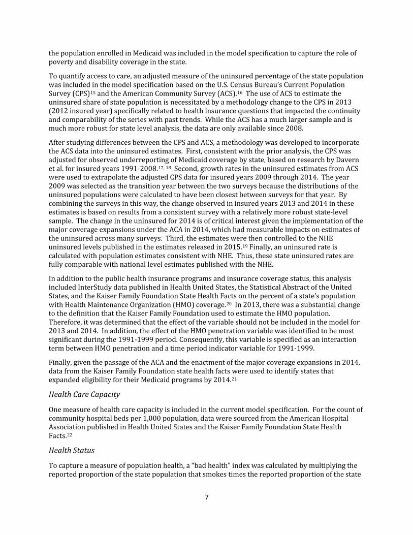
Background and Literature Review The map below (Exhibit 1) illustrates the extent of state-level variation in per capita personal health care expenditures in 2014. Some of the highest levels of per capita health spending were observed in the Northeast and Mid-Atlantic regions, whereas some of the lowest levels were observed in the Southwest region.
Exhibit 1: Personal Health Care Spending Per Capita by State Of Residence, Calendar Year 2014
SOURCES: U.S. Census Bureau; and Centers for Medicare and Medicaid Services, Office of the Actuary, National Health Statistics Group
While there is a large body of literature devoted to understanding the factors associated with geographic variation in health care spending, much of the focus is on individual-level spending (specifically, per beneficiary spending), sub-state regional spending (such as hospital referral region), and Medicare spending. Only a small subset of this research focuses on state-level variation in health spending, and an even smaller number focus on personal health care spending per capita (for all payers) as in this econometric analysis of the SHEA data.
Among the research studies that focus on state-level spending, several common factors were identified that were associated with variation in the level of state-level health spending. These factors tended to fall into the following major categories: income, provider supply or health care capacity, population demographics, health status indicators, insurance coverage types, insured status, and a measure of time (such as a time trend or period fixed effects). A state- level price proxy is also included in some cases (although such a variable is not readily available, so proxies are used to attempt to identify some of the variation associated with price). On the other hand, some studies use national inflation measures, given that a standard state level price index is not readily available. An overview of relevant studies with detailed factors is included in Exhibit 2.

4
Exhibit 2: Research on Geographic Variation in Health Care Spending
Study Year Authors Title Analysis
Measure of Variation / Dependent
Variable
Explanatory Factors Level of data aggregation
2004 DiMatteo
The macro determinants of health expenditure in
the US and Canada: assessing the impact of
income, age distribution, and time
Regression analysis
Real personal health care spending per
capita Income, age, region indicators, time indicators State
2008 Congressional Budget Office
Geographic Variation in Health Care Spending
Regression analysis
Per enrollee Medicare Spending Income Metropolitan
Statistical Area
2009 Acemoglu,
Finkelstein, Notowidigdo
Income and Health Spending: Evidence from
Oil Price Shocks
Regression analysis,
Instrumental Variable
regression
Hospital spending per region/state,
Hospital spending divided by
utilization weight for the population
Income per region (oil reserves as instrument) and Gross Domestic Product by state, state and period fixed
effects
Economic Sub Regions, State
2010 Baker, Bundorf, Kessler
HMO Coverage Reduces Variations in the Use of
Health Care Among Patients Under Age Sixty-
Five
Coefficients of variation and tests
of equality by insurance type on risk adjusted data
(based on regression analysis)
Utilization measures in under
65 population
Type of private health insurance coverage; Risk adjustment controlled for race, sex, age, income, and
area fixed effects Enrollee
2010
Chernew, Sabik, Chandra,
Gibson, Newhouse
Geographic Correlation Between Large-Firm
Commercial Spending and Medicare Spending
Descriptive analysis,
Correlations of utilization and
spending metrics between Medicare (risk adjusted) and
Private payers.
Medicare and Non-Medicare spending and utilization per
capita
Age, sex, and race Hospital Referral Region
2010 Franzini, Mikhail, Skinner
McAllen And El Paso Revisited: Medicare
Variations Not Always Reflected In The Under-
Sixty-Five Population
Descriptive analysis,
comparison of Medicare (risk adjusted) and Private Health
Insurance spending and use
Medicare and Private Health
Insurance: Medical spending per
enrollee, Cost per unit, Use per
enrollee
Age, sex, race, regional Medicare price deflator based on prior research, Medicare hospital wage index
Hospital Referral Region
2010
Gottlieb, Zhou, Song, Andrews,
Skinner, Sutherland
Prices Don't Drive Regional Medicare
Spending Variations
Descriptive analysis of
spending (adjusted for risk and price level differences)
Medicare medical spending per capita,
average usage Price, age, sex, race Hospital Referral
Region
2010 Mittler, Landon, Fisher, Cleary,
Zaslavsky
Market Variations in Intensity of Medicare
Service Use and Beneficiary Experiences
with Care
Correlations, Regression
analysis
End-of-life spending and use per enrollee
Controls for spending and intensity of use included price, age, sex, race and illness; Additional controls for patient perception of care were age, education, health
status, regional effects, Medicare Advantage penetration
Hospital Referral Region
2010
Phillipson, Seabury,
Lockwood, Goldman,
Lakdawalla
Geographic Variation in Health Care: The Role of
Private Markets
Regression analysis
Spending and Use for Medicare and
Private Health Insurance enrollees
Age, sex, income, health status, period and area fixed effects
Metropolitan Statistical Area
2010 Rettenmaier, Saving
Perspectives on the Geographic Variation in
Health Spending
Regression analysis,
Instrumental Variable
regression, Regression on
means over time
Personal health care spending per capita, Medicare spending per enrollee, Non-
Medicare-Non-Medicaid spending
per capita
Income, age, sex, race, educational attainment, bad health index (% current smoker*% obese), health
sector wage, share under 65 population that is uninsured, state fixed effects
State
2010 Rettenmaier, Wang
Regional Variations in Medical Spending and
Utilization: A Longitudinal Analysis of US Medicare Population
Regression analysis (pooled
and rolling annual regressions), coefficient of
variation
Medicare real spending per
enrollee, Utilization
Age, sex, race, death rate, proportion living in an urban area, educational attainment, income, income
inequality, active non-federal physicians per state, per capita number of community hospital beds, trend (for
pooled regressions), indicator variables for various Medicare policy changes; price proxies developed from
national PCE index from the BEA combined with regional price index from the BLS.
State
2010 Wright, Ricketts
The road to efficiency? Re-examining the impact
of the primary care physician workforce on health care utilization
rates
Regression analysis
Various utilization measures per 1,000
population
Proportion primary care physicians (of total physicians), physician density, population density, age,
sex, race, income, per capita number of community hospital beds
Metropolitan Statistical Area,
County
2010
Zuckerman, Waidmann, Berenson,
Hadley
Clarifying Sources of Geographic Differences in
Medicare Spending
Regression analysis
Medicare real spending per
enrollee
Demographics (age, sex, urban and rural shares of the population, race or ethnic group), health status (self-
reported, smoking, body-mass index, prior diagnosis), family income groups, share with supplementary
health insurance, supply variables (share physicians in primary care, number of physician and hospital beds per 1000 population, number of residents per bed,
proximity to a teaching hospital)
Enrollee

5
Study Year Authors Title Analysis
Measure of Variation / Dependent
Variable
Explanatory Factors Level of data aggregation
2013 Chen, Okunade, Lubiani
Quality-Quantity Decomposition of Income Elasticity of U.S. Hospital Care Expenditure Using State-Level Panel Data
Regression analysis
Real hospital spending per capita
Income, inpatient days, hospital characteristics, age, insurance coverage rate by type and status, time trend State
2015 Bose
Determinants of Per Capita State-Level Health
Expenditures in the United States: A Spatial
Panel Analysis
Regression analysis (spatial panel models)
Real hospital spending per capita
Income (Gross Domestic Product by state), insurance coverage, Medicaid expenditures, counts of physicians and hospitals/beds per state population, poverty rate,
age, uninsured rate, unemployment rate
State
2015 Herring, Trish
Explaining the Growth in US Health Care Spending
Using State-Level Variation in Income,
Insurance, and Provider Market Dynamics
Regression analysis,
autoregressive process
Real personal health care spending per
capita
Income, poverty rate, unemployment rate, health insurance coverage rates by type, uninsured rate,
supply measures (counts of physician, hospital beds, market concentration indicators), regulatory indicators
(related to malpractice), self-reported health status, percent of population living in nonmetropolitan area,
autoregressive parameter, state fixed effects
State
Source: Office of the Actuary, National Health Statistics Group; Complete citations are listed in the Appendix section at the end of the paper.
In addition to identifying key factors associated with geographic variation in state-level health spending, there were also other technical challenges to consider in the initial design of this econometric analysis. The first is related to the state-level unit of analysis. Specifically, modeling at the state level involves the use of average metrics versus individual level metrics, which results in higher levels of multicollinearity and endogeneity. For example, the number of physicians in a state may not be related to an individual’s income, but it may be related to the attractiveness of a state’s overall average per capita personal income to physicians or workers in general.4
Another challenge is the time-series-cross-sectional structure of our dataset: 50 state units for each year. The nature of the data set, as well as a Hausman test, suggested the use of a fixed effects model, which accounts for cross-sectional units (such as states) that are consistently geographically fixed over time, as opposed to random effects, which assume a randomly sampled population.6 However, state fixed effects are correlated with many state-level variables that do not change substantially over time, and thus the coefficients for these variables cannot be estimated efficiently using fixed effects models, creating a trade-off between the advantages of fixed effects and capturing the effects of slow moving variables.4 Finally, though state fixed effects models can reduce serial correlation, the method will not necessarily eliminate it. Researchers have used various other tools to address serial correlation (such as adding in autoregressive terms or lagged dependent variables), but those methods (dynamic models) inherently change the research question and modeling approach from a spending level focus to a growth focus.
As a result of these econometric challenges, a number of modeling approaches have been employed in this analysis. Both pooled and fixed effects models are estimated, in addition to a “between” model (a model based on the means by state over time), annual regressions, and several other modeling variants that are constructed to provide sensitivity testing to changes in methodology.7 Based on the broad perspective that these models provide, the factors that are most robust across methods are identified and discussed in this analysis.

6
Data In addition to State Health Expenditure Accounts (SHEA) and enrollment data compiled by OACT, several other state-level characteristics are also incorporated into this econometric analysis. The various sources are discussed in more detail below.
State Health Expenditure Accounts The SHEA data are a subset of the National Health Expenditure Accounts (NHEA) and represent a consistent set of estimates that utilize the same methodology for all states and all years.3 The SHEA are based on the Personal Health Care (PHC) component of the NHEA, which is defined as total spending on health care goods and services; however, it is important to note that PHC (and therefore the SHEA) exclude several NHEA categories: administration and the net cost of private health insurance, government public health activities, and investment in research, structures, and equipment.3
Some SHEA data are excluded from the analysis due to outlier behavior or limited availability. The District of Columbia was excluded from the modeling dataset, as it was an outlier in interstate flows of health spending, health spending per capita, and multiple indicators related to health spending (consistent with the prior analysis).8 Though OACT has developed estimates of private health insurance spending, the data are only available from 2001-2014, and thus it is not incorporated into the modeling and analysis presented here.
In addition to SHEA data, OACT also prepares estimates of Medicare and Medicaid enrollment by state using the latest available source data at the time of estimation.9 The use of enrollment data as part of the model specification is discussed further in the next section.
Exogenous Data
Personal Income and Price Proxies
Personal income per capita was calculated using total personal income by state from the Bureau of Economic Analysis (BEA)10 divided by U.S. Census Bureau’s state population estimates from July of 2016.11 Both income and health expenditures were deflated using the chain-weighted Personal Consumption Expenditures (PCE) price index from the BEA.
Data from the BEA on Regional Price Parities (RPPs) were also utilized in this analysis to study the effects of state variation in prices. These data are not specific to industry and cover a limited period (2008-14); thus in order to have an index that covers the entire sample, the data were additionally back cast to 1991.12,13 These data have evolved from preliminary research and analysis that had been conducted by analysts at the BEA on RPPs, which OACT used in the prior analysis in combination with a regional Consumer Price Index from the US Bureau of Labor Statistics as a proxy for a regional price deflator.4,14 In the current analysis, these RPPs were combined with the Personal Consumption Expenditure Deflator to develop an implicit regional price deflator consistent with the BEA’s calculations used to estimate real personal income by state.13 Ideally, the current analysis would have also included a health-specific price parity, but such data were not available.
Insurance and Coverage-Related Factors
The model specification also includes several categories of insurance coverage type and status. First, the share of the population enrolled in Medicare was included in the model specification to primarily capture the role of the elderly population on state level spending. Second, the share of
7
the population enrolled in Medicaid was included in the model specification to capture the role of poverty and disability coverage in the state.
To quantify access to care, an adjusted measure of the uninsured percentage of the state population was included in the model specification based on the U.S. Census Bureau’s Current Population Survey (CPS)15 and the American Community Survey (ACS).16 The use of ACS to estimate the uninsured share of state population is necessitated by a methodology change to the CPS in 2013 (2012 insured year) specifically related to health insurance questions that impacted the continuity and comparability of the series with past trends. While the ACS has a much larger sample and is much more robust for state level analysis, the data are only available since 2008.
After studying differences between the CPS and ACS, a methodology was developed to incorporate the ACS data into the uninsured estimates. First, consistent with the prior analysis, the CPS was adjusted for observed underreporting of Medicaid coverage by state, based on research by Davern et al. for insured years 1991-2008.17, 18 Second, growth rates in the uninsured estimates from ACS were used to extrapolate the adjusted CPS data for insured years 2009 through 2014. The year 2009 was selected as the transition year between the two surveys because the distributions of the uninsured populations were calculated to have been closest between surveys for that year. By combining the surveys in this way, the change observed in insured years 2013 and 2014 in these estimates is based on results from a consistent survey with a relatively more robust state-level sample. The change in the uninsured for 2014 is of critical interest given the implementation of the major coverage expansions under the ACA in 2014, which had measurable impacts on estimates of the uninsured across many surveys. Third, the estimates were then controlled to the NHE uninsured levels published in the estimates released in 2015.19 Finally, an uninsured rate is calculated with population estimates consistent with NHE. Thus, these state uninsured rates are fully comparable with national level estimates published with the NHE.
In addition to the public health insurance programs and insurance coverage status, this analysis included InterStudy data published in Health United States, the Statistical Abstract of the United States, and the Kaiser Family Foundation State Health Facts on the percent of a state’s population with Health Maintenance Organization (HMO) coverage.20 In 2013, there was a substantial change to the definition that the Kaiser Family Foundation used to estimate the HMO population. Therefore, it was determined that the effect of the variable should not be included in the model for 2013 and 2014. In addition, the effect of the HMO penetration variable was identified to be most significant during the 1991-1999 period. Consequently, this variable is specified as an interaction term between HMO penetration and a time period indicator variable for 1991-1999.
Finally, given the passage of the ACA and the enactment of the major coverage expansions in 2014, data from the Kaiser Family Foundation state health facts were used to identify states that expanded eligibility for their Medicaid programs by 2014.21
Health Care Capacity
One measure of health care capacity is included in the current model specification. For the count of community hospital beds per 1,000 population, data were sourced from the American Hospital Association published in Health United States and the Kaiser Family Foundation State Health Facts.22
Health Status
To capture a measure of population health, a “bad health” index was calculated by multiplying the reported proportion of the state population that smokes times the reported proportion of the state

8
population that is obese (multiplied by 100), based on Behavioral Risk Factor Surveillance System survey data from the Centers for Disease Control and Prevention (CDC)23; this index ideally captures the intersection of residents that share these two unhealthy behaviors by state.24 To assess the reasonability of this conceptual metric, a comparison was made between the bad health index value and the value obtained from a 2006 study, which measured the co-occurrence of these two behaviors on a national basis.25 The researchers from the 2006 study used data from the National Health Interview Survey and found overlap between the populations that are obese and smoke (4.7 percent of the U.S. population on average in 2002), a finding similar to the overlap indicated by the bad health index estimates (cross-state estimated average of 5.2 percent for the same year).25 In addition, the bad health index was also compared with the age-adjusted death rates from the CDC’s National Vital Statistics Reports for 2013 and 2014.26 For both years, there was a relatively high correlation (88.1 percent for each year), suggesting that the bad health index is related to severe health conditions and is not an unreasonable metric to use to control for health status.
See Exhibit 3 below for details on these variables and their associated descriptive statistics.
Exhibit 3: Dependent Variable and Independent Variables Selected for Per Capita Personal Health Care Model, Descriptive Statistics, (1991-2014)
Independent Variables N Mean Std.
Dev. Min Max Personal health care spending per capita, adjusted by the PCE deflator to 2009 dollars
1200 $5,627 $1,489 $2,841 $10,136
Personal Income per capita, adjusted by the PCE deflator to 2009 dollars
1200 $35,341 $7,038 $19,929 $61,305
Community hospital beds per 1,000 population 1200 3.1 1.0 1.7 7.0
Percent of the population enrolled in Medicare 1200 14.7 2.4 4.7 22.5
Bad health index (smoking rate*obesity rate) 1200 4.7 1.5 1.5 9.6
Percent of the population that is uninsured 1200 12.2 3.9 4.2 25.7
HMO penetration (percent of the population by state with coverage from a Health Maintenance Organization)
1200 17.8 12.1 0.0 59.7
Percent of the population enrolled in Medicaid 1200 13.2 4.8 3.2 33.7

9
Methods Several variations of multivariate regression models were estimated to study the relationship between state level characteristics with geographic variation in health spending and also the robustness of these state characteristics across various estimation methods. The base model is estimated via Ordinary Least Squares (OLS), both with state fixed effects (fixed effects model) and without state fixed effects (pooled model). The structure of these models are as follows:
Fixed Effects Model
Yi,t = α + βXi,t + δTrendt + γStatei + νi,t
Pooled OLS Model
Yi,t
= α + βXi,t
+ δTrendt + μ
i,t
Yi,t is the natural log of per capita total health care expenditures deflated by the PCE price index by state i(excluding District of Columbia) and year t (t = 1991 to 2014). Xi,t is a vector of the state-specific characteristics described in the previous section and Exhibit 3. Trendt is a linear time trend. Statei denotes binary indicator variables for each of the states (i = 1 to 50), and vi,t and μi,t represent the error terms for the fixed effects and pooled models, respectively. In addition, clustered standard errors were utilized to account for cross-sectional (contemporaneous) correlation and heteroskedasticity.
Additional sensitivity analysis specific to time-series-cross-sectional data was conducted to understand the robustness of various state factors effects across methods: 1) a “between” model, in which the mean of the dependent variable is regressed on the means of the independent variables, and 2) a set of incremental, annual regressions covering the full timeseries. In the “between” and annual models, the model specification is identical to the pooled model shown above and applied to 50 state observations. The standard errors calculated under both of these approaches were adjusted using the White correction for heteroskedasticity. The goal of estimating these variants related to the time dimension of the data is to understand the potential effects of serial correlation on variable significance when the time dimension is either removed from or transformed in the data set.
Finally, variants of the pooled and fixed effects models were studied to understand the implications of the newly available data for regional prices, the recent recession, and the major coverage expansion under the ACA on variation in health spending. First, to estimate the regression incorporating the regional price data, personal health care spending per capita and personal income per capita were both divided by the overall RPP series (for all goods and services) and then by the PCE deflator series.13 This adjustment ideally deflates these spending series into real dollars that account for regional price differences over time. Second, to study the recession, the pooled and fixed effects models were estimated over differing time periods; in addition, there were also regressions based solely on income (to isolate economic impacts). Third, regressions were estimated to study the effects of the 2014 coverage expansions. In these regressions, several variables were added to the specification such as interactions of a 2014 indicator variable with key variables that would be inherently effected by the ACA (i.e. the share of the population that is uninsured and the share that is enrolled in Medicaid).

10
Revisions to the Model Specification Though this analysis largely builds from the prior published analysis on state health spending data by OACT,4 relationships between the state characteristics and state health spending change over time. As such, the econometric work has been updated to reflect both revisions in the data and the extended sample period. Accordingly, in the process of updating the prior OACT analysis, some variables were removed from the specification, while new ones were added (variables included in current specification are described in Exhibit 3). Despite these changes, the model specification is rather similar to that from the prior econometric analysis. Exhibit 4 provides a comparison between the previously published OACT pooled and fixed effects models (models [A] and [B]) with the revised models (models [C] and [D]). These changes are also described in the following paragraphs.
Three state demographic characteristics were removed from the prior model specification. The first variable removed was the gender variable (women aged 20-44 as a share of the state population), which was meant to capture the effects on health spending associated with women of child bearing age.4 During the previous analysis, this variable was observed to be the most negatively trended variable in the data set (due to the declining trend of baby-boomers in this group as they aged through the 1991-2009 period). Despite an a priori expectation of relatively higher spending associated with this group for child birth related health expenditures, the coefficient for this variable was previously found to be negative in regression analysis with fixed effects (although positive in the previous pooled model). Since the last analysis, the declining trend in the series has become more severe. Accordingly, it appears that the variable is mostly capturing an effect of age combined with the declining trend of baby boomers in this group and, as a result, the variable was removed from the specification. Second, the variable representing race was also removed from the specification (specifically, the share of non-Hispanic, African Americans of the state population). In the prior regressions, this variable was marginally significant across various regression methods. With the new and revised data, this variable was not identified to be significant across several methods and was thus removed from the specification. Third, the elderly share of the population was removed from the specification and replaced with a more specific Medicare coverage variable (discussed further below).
On the other hand, two new variables were added to the specification during this update. First, the share of the state population over 65 years of age was replaced with the share of the state population enrolled in Medicare. The share of the state population enrolled in Medicare is more closely related to state health spending than the share of the elderly population, since it is a more direct measure of health insurance coverage. Interestingly, the estimated effect of these two variables is nearly identical, but more significant for the Medicare share variable than the elderly share variable, which is intuitive given there is essentially universal coverage for this age group. Second, the share of the population enrolled in Medicaid was added. This addition was a function of two key factors: the need to capture varying access to care across states for low income individuals (and those eligible who are aged or disabled) and the need to capture the effects of the Medicaid expansion in 2014.

11
Exhibit 4: Comparison of Prior Published Models with Revised Models
[A] [B] [C] [D]
Dependent Variable: Log of Total PHC Spending Per Capita (2009$)
Previously Published Pooled Model† Previously Published
Fixed Effects Model† Pooled Model Fixed Effects Model
Independent variables Coef.(Std.Err.) Coef.(Std.Err.) Coef.(Std.Err.) Coef.(Std.Err.) Constant 1.047*** (0.210) 4.306*** (0.596) 0.266* (0.191) 1.078** (0.628) Log of Personal Income per capita (2009$) 0.598*** (0.018) 0.426*** (0.062) 0.718*** (0.018) 0.641*** (0.059) Community Hospital Beds per 1,000 population 0.019*** (0.003) 0.034*** (0.012) 0.024*** (0.002) 0.025** (0.014) % of Population enrolled in Medicare - - 0.020*** (0.001) 0.010* (0.007) Bad Health Index (%Smoker*%Obese*100) 0.023*** (0.004) 0.008*** (0.004) 0.017*** (0.003) 0.006 (0.005) % Uninsured Population -0.001* (0.001) 0.000 (0.001) -0.001* (0.001) 0.008*** (0.002) % HMO Population*Dummy Variable (1991-1999)† -0.001*** (0.000) -0.002*** (0.000) -0.001** (0.001) -0.001** (0.001) % of Population enrolled in Medicaid - - 0.006*** (0.001) 0.004*** (0.001) Time Trend 0.027*** (0.002) 0.022*** (0.003) 0.014*** (0.001) 0.019*** (0.002) % of Women aged 20-44 0.029*** (0.009) -0.040*** (0.006) - - % of Non-Hispanic African Americans -0.001* (0.001) 0.001 (0.004) - - % of Population over 65 years 0.029*** (0.002) 0.016*** (0.006) - - Sample 1991-2009 1991-2009 1991-2014 1991-2014 n 950 950 1200 1200 Adjusted R-squared 0.890 0.973 0.921 0.969
Notes: Personal Consumption Expenditure (PCE) deflator was used to adjust spending to 2009 dollars. Coefficients and standard errors (in parentheses). Standard errors are adjusted for cross-equation (contemporaneous) correlation as well as different error variances in each cross-section (heteroskedasticity). Numbers with ***, **, and * are significant at the 5%, 10%, and 20% levels, respectively. †Note, that for the HMO population variable, the full sample of HMO data was used in the estimate (1991-2009) for models [A] and [B}. Thus, for models [A] and [B], there was not an interaction term used for the HMO variable.

12
Results Overall, the various regression methods conducted suggest that several state characteristics are important for understanding geographic variation in health spending. The factors that are most robust across modeling methods are personal income per capita, the share of the population enrolled in Medicare, the share of the population enrolled in Medicaid, the supply of community hospital beds, and the share of the population that is uninsured. Health status and HMO penetration are less robust to changes in methodology. Detailed results for the current pooled and fixed effects models are shown above in Exhibit 4. The results for the between and annual models are shown in Exhibits 5 and 6, respectively.
Pooled Model Consistent with research on national-level health spending patterns over time, measures of income (personal income per capita) and indicators of technology (captured by the linear time trend) are highly significant factors explaining variation in state-level health care spending. 27,28 Although per capita income is intended to measure differences in state resources to pay for health care, due to the lack of a state or regional price measure, the cross-state income effect estimated also includes a pricing effect (discussed in more detail below). As a result, the reasonableness of our income coefficient (0.718) was assessed based on comparisons with coefficients estimated in similar studies on cross-state or subnational income elasticity (which tended to range from 0.5 to 0.724,29,30).
Notably, compared to previous OACT estimates, the cross-state income elasticity estimated with data through 2014 substantially increased in magnitude. This change occurs even if 2014, the year of the major coverage expansions under the ACA, is excluded. While some of this change is due to data and model revisions, this change also coincides with the most recent recession and associated modest recovery, which was followed by the slowest rates of growth in health spending observed over the history of the NHE accounts data. In this context, the revised elasticity estimate does not seem unreasonable.
The inclusion of a linear time trend suggested roughly a 1.4-percent increase in health spending per year (implicitly associated with technological advances), which was lower than that observed among some earlier studies that estimate separate income and time trend coefficients in health spending regressions. 24, 27 It was also lower compared to OACT’s prior analysis on state health spending.4 Similar to the cross-state income elasticity, the trend also seems to have been influenced by the recession and the historically low health spending growth that occurred in the years that followed. While this current analysis includes this post-recession period, other studies largely do not.
The share of the state population enrolled in either Medicare or Medicaid was associated with relatively higher state spending levels. A one percent increase in the share of the state population enrolled in Medicare is associated with an estimated increase in real personal health care spending per capita of 2.0 percent. This is slightly lower than the coefficient estimated in OACT’s prior pooled model regression for relative spending associated with the share of the population over 65 years of age. However, the change in the magnitude of the coefficient is likely the net effect of several factors. Contributing to a lower magnitude in the coefficient, per beneficiary growth over 2010-14 was the lowest observed in the history of the program.31 Underlying the slow growth were legislated payment update reductions to Medicare providers, low provider payment updates related to the recession, and Medicare-specific policy and legislative factors that also impacted spending growth (such as the readmission program and the two-midnight policy).32,33 In addition,
13
the entrance of the baby-boom generation into the program over this period substantially contributed to the program’s enrollment growth, but at the same time brought the average age of the beneficiary down (implying relatively less spending per new beneficiary on average), which would tend to dampen the magnitude of the coefficient that measures the effect of coverage over time. Conversely, replacing the elderly share of the state population with the Medicare enrollment share tends to increase the magnitude of the coefficient (as the variable is more directly associated with health spending for this population and also includes a small share of the beneficiary population who qualifies for the program but is under age 65).
Similarly, a 1-percent increase in the share of the state population enrolled in Medicaid is associated with a relative increase in real personal health care spending per capita (of 0.6 percent). The relatively lower coefficient magnitude compared to that of Medicare seems reasonable given the differences in spending for each program on a per capita basis (which would implicitly include effects from Medicaid’s lower relative provider payment rates compared to Medicare). Medicaid spending on personal health care per capita is 27 percent lower than Medicare (in 2013), which implies that the coefficient should also be lower for Medicaid (since the coefficient is measuring an impact on overall spending per capita). The coefficient magnitude is actually estimated to be lower by 71 percent, however. This additional difference in coefficient magnitudes is likely somewhat explainable by the effect of dual enrollees (people who are enrolled in both Medicare and Medicaid, who tend to spend more on health care than younger, non-disabled Medicaid enrollees), which suggests that some of the effect of Medicaid coverage might also be captured in the estimated Medicare enrollment coefficient. This is further supported by the 1991-2013 correlation between the two variables (sample correlation is significant at 38.3 percent). While the correlation is statistically significant, it was not found to be high enough to suggest removal from the model specification.
On the other hand, the lack of insurance, as measured by the share of the population that is uninsured, was associated with a relative decrease in personal health care spending per capita. A 1-percent increase in the share of the uninsured of the state population was associated with a 0.1-percent decline in real personal health care spending per capita. In the pooled model, this factor was marginally significant, but in the between model and annually estimated models (discussed later), this variable was found to be highly significant, particularly during this most recent recession. The negative coefficient likely reflects limited access to and resources to pay for medical care due to lack of insurance coverage.24 The recession had a notable impact on health spending not only through slower growth in income or slower growth in inflation, but also due to the large loss of employment and thus access to employer-sponsored insurance.34
A 1-percent increase in the share of state residents enrolled in an HMO (from 1991-1999) was associated with a 0.1-percent decrease in health spending, likely related to HMOs’ tighter management of health care utilization relative to other types of insurance.35,36 The choice to include the interaction of the HMO variable with the 1991-1999 period variable reflects the period in which HMOs’ impact on utilization and health spending was most substantial. It also removed the impact of the change in the HMO data series definition in 2013.
Community hospital beds per 1,000 population, which is a measure of health care capacity, was estimated to have a positive estimated coefficient. An increase of one hospital bed per 1000 population was associated with an estimated 2.5-percent increase in real personal health care spending per capita by state. This coefficient magnitude is in line with the previous OACT pooled regression. In addition, other researchers identified comparatively higher health spending for certain insured populations where there were higher concentrations of hospital beds.37

14
Finally, consistent with prior analysis, the bad health index also had an estimated positive sign, indicating higher medical costs in states with higher shares of residents with relatively lower health status. Thus, a 1-percentage point increase in the bad health index (smoking rate * obesity rate * 100) was associated with an estimated 1.7-percent increase in real personal health care spending per capita by state. As discussed earlier in the paper, OACT has found a high correlation (about 88 percent) with the age-adjusted death rate with the bad health index (over several years), which bolsters its usefulness as a health status indicator. Since the last analysis, rates of obesity have continued to increase and also have demonstrated an increasing correlation with the time trend.23 Thus, the approach of using the interaction term between obesity and smoking rates tends to reduce multicollinearity.
Fixed Effects Model Consistent with our prior analysis, an F-ratio test indicated that the fixed effects coefficients are statistically significant versus the assumption that the constant is shared across the states.4 This was expected given the limited number of state-level variables available. However, as stated previously, state fixed effects are likely to be correlated with slow moving state characteristics of interest. As such, it is expected that not all of the variables in the specification will be robust to both the pooled and fixed effects models. Accordingly, the results showed that while most factors were robust to both methods, two factors became either insignificant or inconsistent with theory.
As was the case in previous analysis, the cross-state income elasticity estimated in the fixed effects model remained highly significant. However, contrary to prior OACT analysis, the coefficient for the variable declined only slightly from 0.718 to 0.641 (a 0.08 difference from the pooled model compared to the prior analysis through 2009 that exhibited an estimated difference of 0.17). In prior analysis, the reduction in the income elasticity between the pooled and fixed effects models was thought to be related to state fixed effects potentially picking up price variation across states. Interestingly, this change in the divergence between models looks to be largely a function of the addition to the sample of the post-recession period, in which health spending growth and medical inflation rates were historically low as indicated earlier. If the revised data and model are used in a regression, but limited to 1991-2009, the pattern of the larger differential between the pooled model income coefficients (0.667) and the fixed effects model income coefficient (0.398) observed in the prior OACT analysis holds. Overall, this might be an indication that price variation was reduced during the recession. Additional analysis conducted with the limited data available on the regional price parities is discussed in more detail below. In general, the ability of this variable to explain most of the variation in health spending between states (in and of itself) and its statistical significance between models supports the robustness of this factor to both methods.
In addition to income, several other factors retained significance (or had only minor losses in significance) and had somewhat similar coefficient magnitudes between the pooled and fixed effects models. This suggests that these factors were more robust to the inclusion of fixed effects. The coefficient for the number of community hospital beds per 1,000 population was nearly identical between the pooled and fixed effects models. Coefficient magnitudes for the shares of the state population enrolled in Medicare and Medicaid were slightly lower, while the magnitude of the trend coefficient increased slightly, although all remained in a similar order of magnitude.
Conversely, some independent variables from the pooled model specification either became insignificant or had estimated coefficients inconstant with theory in the fixed effects model. In the fixed effects model, the bad health index exhibited a substantial loss in significance, indicating that the factor is not robust to this method. In addition, while the uninsured share of the state population retained significance, its coefficient changed signs, which is counter to the theory for

15
inclusion into the specification. In the pooled model, an increase in the uninsured is associated with a decrease in health spending, while in the fixed effects model, the opposite occurs, which suggests that this factor is less robust to the fixed effects specification.
As discussed earlier, since fixed effects ideally represent regional characteristics that do not change over time, they interact with exogenous state-level characteristics that also do not change substantially over time. The current set of independent variables vary little over time, particularly when compared to the variation across states. An analysis of the coefficients of variation (COV), measured by the ratio of the standard deviation to the mean, was used to demonstrate the difference in period-specific and cross-sectional specific variation. For all variables that were included in the model specification, the cross-sectional variation exceeded period-specific variation. As such, the addition of state fixed effects to the model would be expected to greatly increase the multicollinearity in the model and thus make these coefficients more difficult to estimate efficiently. Consequently, the addition of fixed effects resulted in a loss of significance and an unreasonable change in sign for two factors in the specification.
Between Model The “between” model was estimated using the means of all the variables over time (see results in Exhibit 5 below). The between model is conceptually similar to the pooled model, but attempts to remove the element of time from the regression and thus theoretically addresses two key issues: 1) it removes the need for fixed effects and associated multicollinearity between state fixed effects and the independent variables and 2) it also removes relationships with prior period variables and consequently, serial correlation arising from slow-moving variables. However, this technique is not as useful for examining periodic effects, such as economic cycles, and the use of the mean for each variable makes it more challenging to identify statistically significant relationships. Therefore, while the “between” model results were somewhat similar to those of the pooled model, some variables become only marginally significant or insignificant.
Despite the challenges, this alternative modeling approach helps to identify which independent variables have relatively more robust relationships with variation in health spending. Accordingly, several variables remained highly significant with rather similar estimated coefficient magnitudes: real personal income per capita, the share of the population enrolled in Medicare, the share of the population enrolled in Medicaid, and the share of the population that is uninsured. Given that income has previously shown robustness across various methods, it’s not surprising to find that it remains robust in this method. In addition, the public coverage variables would be expected to have a strong and consistent relationship with health spending variation since they are directly related to health spending. However, the uninsured variable is more cyclical in nature. Thus, in one sense, it is somewhat surprising to see this variable remain highly significant in this method; although, this factor’s importance in this setting may be an indication of the severity of the recent recession and modest recovery that followed, which coincided with substantial losses of coverage during and just after the recession.
The count of community hospital beds and the bad health index both became less statistically significant in this method, although the estimated coefficients were similar. While not quite as robust as the other factors, the marginal significance does suggest that these factors are still important to consider in explaining geographic variation in health spending. On the other hand, the estimate of the coefficient for HMO penetration showed a substantial decline in significance. This is not too surprising given that the effect is expected to be concentrated in the 1990s and would thus be diminished when averaged over time, which further supports limiting this variable’s effects to the 1990s in the pooled model.

16
Exhibit 5: Comparison of Pooled and Between Models [A] [B]
Dependent Variable: Log of Total PHC Spending Per Capita (2009$) Pooled Model1 Between Model2,3
Independent variables Coef.(Std.Err.) Coef.(Std.Err.) Constant 0.266* (0.191) 0.536 (0.939) Log of Personal Income per capita (2009$) 0.718*** (0.018) 0.728*** (0.094) Community Hospital Beds per 1,000 population 0.024*** (0.002) 0.021* (0.013) % of Population enrolled in Medicare 0.020*** (0.001) 0.018** (0.009) Bad Health Index (%Smoker*%Obese*100) 0.017*** (0.003) 0.020** (0.011) % Uninsured Population -0.001* (0.001) -0.005*** (0.002) % HMO Population*Dummy Variable (1991-1999) -0.001** (0.001) -0.001 (0.001) % of Population enrolled in Medicaid 0.006*** (0.001) 0.008*** (0.003) Time Trend 0.014*** (0.001) - Sample 1991-2014 Average over 1991-2014 n 1200 50 Adjusted R-squared 0.921 0.742
Notes: Personal Consumption Expenditure (PCE) deflator was used to adjust spending to 2009 dollars. Coefficients and standard errors (in parentheses). Numbers with ***, **, and * are significant at the 5%, 10%, and 20% levels, respectively. 1Standard errors are adjusted for cross-equation (contemporaneous) correlation as well as different error variances in each cross-section (heteroskedasticity). 2Standard errors are adjusted for heteroskedasticity using the White correction. 3For the "Between" model, all variables were averaged over 1991-2014 to obtain a sample of 50 average values by state for the dependent and independent variables. "Pooled" model, the HMO variable was only included for 1991-1999.
Annual Models Another method to test the robustness of these state characteristics is an approach in which 24 year-specific regressions are estimated individually (Exhibit 6). Since the time dimension is estimated separately, state fixed effects are not needed and serial correlation is removed. Like the between model, this approach is meant to remove some of the inefficiencies created by slow-moving variables combined with the inclusion of fixed effects. On the other hand, unlike the between model, this approach allows for the tracking of time-related effects by looking at the change in coefficient estimates and their significance incrementally over time. Hence, this method allows for the possibility that various factors will be more or less important during different periods within the overall sample. Consistent with prior analysis, the resulting coefficient magnitudes were more comparable to the pooled model (versus the fixed effects model), suggesting that the pooled model explains mostly cross-sectional variation.
Accordingly, there was fluctuation in the magnitudes and/or significance of the estimated coefficients over time for all of the variables in the model. As seen previously, the income coefficient was highly significant over time and the coefficient ranged from 0.6 to 0.8 (increasing noticeably after 2008), which was close to the pooled model estimate of 0.718. The slight increasing trend, particularly after 2008, suggests that this effect is tied to the recession. The data set contains two recessions (the start of the sample at 1991 excludes the beginning of the 1990-1991 contraction). After the 2001 recession, the income coefficient showed a marked uptick in 2002. For the most recent recession, there was another substantial uptick in the magnitude of the income coefficient during the recessionary period, which is not surprising given the substantial decline in income and loss of employment that occurred. Thus, the timing of the responsiveness of health spending to income changes was more immediate in the last recession, which is not surprising given its relative severity.
In addition to income, the variables that were at least marginally significant (at the 20 percent level) for at least half of these regressions include: percent of the state population enrolled in Medicare, percent of the state population enrolled in Medicaid, percent of the population that is uninsured, and community hospital beds per 1,000 population (although the significance of community hospital beds was more concentrated in the earlier part of the sample and less so in later years). The coefficient for the share of the population enrolled in Medicare is somewhat stable overtime, rounding to 0.02 for the majority of the annual regressions (mirroring the magnitude of

17
the pooled coefficient of 0.02). The coefficient for the share of the population enrolled in Medicaid oscillates fairly closely around its average of 0.007 over the 24 periods (rather close to the pooled coefficient of 0.006). Interestingly, the magnitude for the coefficient for Medicaid ticks down slightly during or just after a recession. This may be capturing a cyclical effect of a temporary per enrollee spending trend when an increasing share of relatively less expensive non-aged, non-disabled enrollees (who are comparatively less expensive than the aged and disabled beneficiaries) enter the Medicaid program due to short-term financial difficulty.38 In the 2000s, the uninsured share of the population tended to be more significant with a higher magnitude compared to the coefficient estimated in the pooled regression. This is likely due to the share of the uninsured population reflecting cyclical effects of recent recessions and in 2014, expanded insurance coverage under the ACA; hence, it is inherently capturing two key factors that have substantially impacted health spending in recent years. The coefficients for the count of community hospital beds per capita was most significant in the 1990s and early 2000s, rounding to about 0.03 during those years, compared to 0.024 for the pooled model. The trend in this coefficient during this time is capturing a period of a relative decline in community hospital beds as the population grew, particularly in the 1990s. Given the trend of hospital inpatient services shifting to outpatient services during this time, encouraged by the rapid growth of HMO plans in the 1990s, the decline in capacity and the decline in its ability to explain variation across states, seems reasonable. Consequently, during the most recent portion of the sample, hospital capacity has become less of a significant factor in explaining variation in health spending versus the other economic and age variables. Finally, the bad health index and the share of the population enrolled in a HMO were only occasionally significant, suggesting that these variables are less robust to this change in methodology.
In this method, lower adjusted R-squared estimates were observed compared to the full panel data set regressions, which, as in past analysis, suggests that serial correlation causes some bias in the adjusted R-squared for the pooled models. There also seems to be a cyclical pattern in the adjusted R-squared with relatively higher values occurring during or just after a period of recession, indicating that state-level economic factors become more dominant in explaining health spending variation during periods of economic contraction.

18
Exhibit 6: Individual Year Regressions Dependent Variable: Log of Total PHC Spending Per Capita (2009$)
Independent Variables:
Year Constant
Log of Personal
Income per capita
(2009$)
Community Hospital Beds
per 1,000 population
% of Population enrolled in Medicare
Bad Health Index
% Uninsured Population
% HMO Population
% of Population enrolled in Medicaid
Time Trend
(linear) Adj. R^2
1991 0.852 0.672 0.031 0.013 0.015 0.002 0.002 0.010 - 0.791 1992 0.766 0.676 0.028 0.016 0.023 0.002 0.003 0.009 - 0.783 1993 0.353 0.715 0.031 0.017 0.013 0.003 0.002 0.011 - 0.762 1994 -0.234 0.769 0.033 0.021 0.016 0.003 0.002 0.009 - 0.762 1995 0.251 0.730 0.034 0.022 0.015 0.001 0.001 0.006 - 0.707 1996 0.353 0.726 0.023 0.022 0.014 0.001 -0.001 0.007 - 0.647 1997 1.127 0.651 0.029 0.021 0.017 0.001 0.000 0.005 - 0.623 1998 1.378 0.630 0.031 0.020 0.015 -0.002 0.000 0.006 - 0.659 1999 1.073 0.655 0.027 0.025 0.013 0.000 0.000 0.007 - 0.644 2000 1.056 0.661 0.033 0.023 0.013 -0.001 -0.001 0.006 - 0.663 2001 1.372 0.642 0.033 0.018 0.020 -0.005 -0.001 0.006 - 0.657 2002 0.843 0.698 0.032 0.019 0.018 -0.003 -0.001 0.005 - 0.654 2003 0.731 0.714 0.024 0.021 0.016 -0.004 -0.001 0.005 - 0.640 2004 1.437 0.655 0.018 0.019 0.022 -0.007 -0.001 0.004 - 0.620 2005 1.680 0.646 0.002 0.020 0.014 -0.012 -0.003 0.006 - 0.610 2006 1.957 0.617 0.020 0.017 0.011 -0.010 -0.002 0.007 - 0.623 2007 1.519 0.662 0.008 0.017 0.014 -0.011 -0.002 0.008 - 0.661 2008 1.173 0.687 0.006 0.021 0.007 -0.007 -0.002 0.008 - 0.678 2009 0.660 0.736 0.012 0.023 0.004 -0.004 -0.002 0.007 - 0.727 2010 0.833 0.725 0.011 0.019 0.009 -0.006 -0.002 0.007 - 0.745 2011 0.481 0.752 0.002 0.019 0.018 -0.006 -0.002 0.007 - 0.745 2012 1.074 0.694 0.007 0.021 0.012 -0.005 -0.002 0.007 - 0.682 2013 0.679 0.732 -0.003 0.021 0.019 -0.006 -0.002 0.006 - 0.674 2014 0.913 0.709 0.007 0.021 0.019 -0.005 -0.001 0.004 - 0.631
Notes: Personal Consumption Expenditure (PCE) deflator was used to adjust spending to 2009 dollars. Numbers in bold-italic are significant at the 5% level. Numbers in bold are significant at the 10% level. Numbers in italics are significant at the 20% level. Standard errors are corrected for heteroskedasticity using the White correction. Shaded rows indicate recession periods as indicated by the National Bureau of Economic Research.
Specification Variants
Adjusting for Price
To assess the impact of using a state-level price indicator and to differentiate the impact of regional price trends, additional pooled regressions were estimated using a newly developed state price indicator (RPP) from the BEA. As mentioned earlier, these RPPs were only available over a limited period of time, and were thus back cast to cover the full sample period. The RPPs were then combined with the PCE deflator to obtain an implicit regional price deflator in these regressions. Despite the limited availability, the variable is useful in giving a potential indication of the portion of the cross-state income elasticity that is related to price effects. Results are shown in Exhibit 7.
As expected, the inclusion of a price adjustment (to the income and health spending variables) in the pooled model reduced the income elasticity from 0.718 to 0.652. This mirrors the pattern seen with the magnitude of the reduction of the income elasticity between the pooled and fixed effects model in the current analysis (0.718 in the pooled model to 0.641 in the fixed effects model). Thus, the income elasticity in the regressions where this price adjustment is not included is likely capturing some price effects. On the other hand, in prior OACT estimates with a sample of 1991-2009, both the incorporation of experimental state-specific prices (from 0.598 to 0.429) and the addition of fixed effects to the pooled model (from 0.598 to 0.426) reduced the income elasticity more significantly and by a similar order of magnitude. In a regression with the sample reduced to 2009 (based on revised data), the differential between the price and non-price adjusted income elasticity coefficients increases to 0.111 (0.557 in the price adjusted pooled model versus 0.667 in the non-price adjusted model). This finding suggests that the post-recession period is driving some of the difference in the price adjusted coefficient.

19
Comparing all these results, it appears that the addition of the post-recession period to the sample results in a smaller share of the magnitude of the income elasticity being driven by price variation. During this post-recession period of historically low rates of medical inflation, this reduction in the impact of the price adjustment on the income elasticity suggests that the recession may have resulted in dampened variation in regional price growth. In line with this, the variation in the RPPs has declined after 2008 with their annual coefficients of variation declining from 8.9 percent in 2009 to 8.5 percent in 2013. Recent research by Beraja, Hurst, and Ospina found that the severity of regional recessions was strongly related to local inflation rates.39 Thus, this change in the measured income coefficient when regional price is accounted for between OACT’s prior and current analysis is likely tied to the recession and slow recovery that followed, which experienced a period of historically slow price growth.
Generally, with the exception of the income coefficient, these estimated coefficient and magnitudes for the other variables were similar to those of the pooled model without the price adjustment. In a couple of cases (community hospital beds per 1,000 population and the bad health index), the magnitude of the coefficient increased somewhat, likely indicating some regional price interaction with those variables.
Exhibit 7: Comparison of Current Models with Regional Price Adjusted Models [A] [B] [C] [D] [E] [F]
Dependent Variable: Log of Total PHC Spending Per Capita (2009$)
Pooled Model Fixed Effects Model
Pooled Model Adjusted for
Price
Fixed Effects Model
Adjusted for Price
Pooled Model Not Adj. for
Price (1991-2009)
Pooled Model Adjusted for
Price (1991-2009)
Independent variables Coef.(Std.Err.) Coef.(Std.Err.) Coef.(Std.Err.) Coef.(Std.Err.) Coef.(Std.Err.) Coef.(Std.Err.)
Constant 0.266* (0.191)
1.078** (0.628)
0.865*** (0.289)
0.449 (0.587)
0.694*** (0.173)
1.720*** (0.226)
Log of Personal Income per capita (2009$) 0.718*** (0.018)
0.641*** (0.059)
0.652*** (0.028)
0.699*** (0.056)
0.667*** (0.017)
0.557*** (0.022)
Community Hospital Beds per 1,000 population
0.024*** (0.002)
0.025** (0.014)
0.039*** (0.003)
0.034*** (0.013)
0.027*** (0.002)
0.044*** (0.002)
% of Population enrolled in Medicare 0.020*** (0.001)
0.010* (0.007)
0.020*** (0.001)
0.012** (0.007)
0.021*** (0.001)
0.022*** (0.001)
Bad Health Index (%Smoker*%Obese*100) 0.017*** (0.003)
0.006 (0.005)
0.025*** (0.003)
0.004 (0.005)
0.012*** (0.003)
0.022*** (0.003)
% Uninsured Population -0.001* (0.001)
0.008*** (0.002)
-0.002* (0.001)
0.008*** (0.002)
-0.002** (0.001)
-0.002*** (0.001)
% HMO Population*Dummy Variable (1991-1999)
-0.001** (0.001)
-0.001** (0.001)
-0.001*** (0.001)
-0.001*** (0.001)
0.000 (0.000)
-0.001* (0.000)
% of Population enrolled in Medicaid 0.006*** (0.001)
0.004*** (0.001)
0.005*** (0.001)
0.004*** (0.001)
0.007*** (0.001)
0.006*** (0.001)
Time Trend 0.014*** (0.001)
0.019*** (0.002)
0.015*** (0.001)
0.018*** (0.002)
0.019*** (0.001)
0.022*** (0.001)
Sample 1991-2014 1991-2014 1991-2014 1991-2014 1991-2009 1991-2009 n 1200 1200 1200 1200 950 950 Adjusted R-squared 0.921 0.969 0.922 0.970 0.917 0.921
Notes: Personal Consumption Expenditure (PCE) deflator was used to adjust spending to 2009 dollars. Coefficients and standard errors (in parentheses). Standard errors are adjusted for cross-equation (contemporaneous) correlation as well as different error variances in each cross-section (heteroskedasticity). Numbers with ***, **, and * are significant at the 5%, 10%, and 20% levels, respectively.
The Recent Recession and Regional Variation
As shown throughout this paper, the results across several methods suggest that the severity of the most recent recession and the slow recovery that followed substantially influenced the estimated impact of state economic characteristics on health spending variation. Most notably, the cross-state income elasticity was most responsive to the inclusion of the post-recession period of historically slow personal health care spending growth, particularly in the presence of historically slow inflation rates and declining price variation.
To dig into the effect of the post-recession years on state health spending, supplementary pooled and fixed effects regressions were estimated over different time periods within the available state health expenditure data (Exhibit 8). The two additional periods estimated were 1991-2009 (to compare to the sample in OACT’s prior analysis, which includes the recent recession, but not the

20
post-recession period) and 1991-2013 (to study the impact of the post-recession period, where health spending grew at the lowest rates observed over the history of the NHEA data, but excludes 2014, when substantial policy changes occurred under the ACA). Notably, national personal health care spending per capita grew at the slowest rates in the history of the NHEA accounts for 2010-2013, which is consistent with the pattern of health spending growth following patterns in economic growth with a lag as has been consistently found at the aggregate level.34 However, since these state-level models are focused on level relationships, the effects of the recessions are observed in regional level relationships, but also with a lag. For the pooled models, the estimated income coefficient increased from 0.667 in the 1991-2009 regression to 0.702 in the 1991-2013 regression. More notable is the increase in the income coefficient in the fixed effects model from 0.398 in the 1991-2009 regression to 0.629 in the 1991-2013 regression. Further, the difference in magnitude between the pooled and fixed effects model estimates of the income coefficient (thought to be related to regional price variation captured with the income variable) falls substantially from 0.269 to 0.073 between the 1991-2009 and 1991-2013 regressions. Thus, the inclusion of the post-recession period tends to increase the magnitude of the cross-state income elasticity, suggesting that the effect is sensitive to economic cycles. In addition, as stated earlier, the reduction of the magnitude of the difference between the estimated income elasticity between the pooled and fixed effects models with the inclusion of the post-recession period is consistent with regional price variation playing a smaller role in explaining regional variation in health spending after the recession.
Another way to study the importance of economic factors on health spending is to estimate the share of the geographic variation in health spending explained in a regression in which only economic variables are included in the model. In pooled, state-level regressions (without fixed effects), real personal income per capita explains 58 percent of the geographic variation in health spending by itself, and 82 percent if a trend is included in the specification. This is consistent with the strong relationship observed between health spending and economic growth (income) at the national level.34 Thus, regional patterns in health spending are highly responsive to regional differences in local economic strength. Consequently, the regions that experienced relatively more substantial economic downturns during the most recent recession (with some of the largest decelerations in average personal income per capita spending growth by state) also experienced some of the largest slowdowns in personal health care spending per capita growth over this period.
The importance of economic factors is further supported by the results of incremental, annual regressions, discussed previously, which suggest that during or just after periods of economic contraction, economic factors become even more dominant in explaining health spending variation. To isolate the impact of the economic cycles on the share of variation explained over time, additional annual regressions were estimated over 1991 through 2014 with only income (and a constant). The adjusted R-squared estimates follow a similar cyclical pattern as seen with the annual estimates with the all the variables included in the specification (and are thus not shown here for brevity’s sake). However, the cyclical pattern is more defined in that there is a notable uptick in the adjusted R-squared estimates following recessionary periods. Specifically, there are local maxima in the adjusted R-squared at 2003 and 2010, associated with the 2001 and 2007-2009 recessions, respectively.40 Note that since the SHEA data start at 1991, part of the 1990-1991 recessionary period is truncated. This trend further supports the finding that regional economic growth (here specifically measure by personal income per capita) becomes more important in explaining variation in health spending in the periods following a recession. These results are also indicative of the cyclical underpinnings of the recent slowdown in health spending after the recession.
Exhibit 8: Comparison of Current Models Estimated Over Different Sample Periods

21
[A] [B] [C] [D] [E] [F] [G] [H]
Dependent Variable: Log of Total PHC Spending Per Capita (2009$)
Pooled Model (1991-2009)
Pooled Model (1991-2013)
Pooled Model
(full sample)
Fixed Effects Model (1991-2009)
Fixed Effects Model (1991-2013)
Fixed Effects Model
(full sample)
Pooled Model
(Income Only)
Pooled Model
(Income & Trend Only)
Independent variables Coef. (Std.Err.)
Coef. (Std.Err.)
Coef. (Std.Err.)
Coef. (Std.Err.)
Coef. (Std.Err.)
Coef. (Std.Err.)
Coef. (Std.Err.)
Coef. (Std.Err.)
Constant 0.694*** (0.173)
0.420*** (0.182)
0.266* (0.191)
3.223*** (0.708)
1.205** (0.658)
1.078** (0.628) - -
Log of Personal Income per capita (2009$)
0.667*** (0.017)
0.702*** (0.018)
0.718*** (0.018)
0.398*** (0.070)
0.629*** (0.062)
0.641*** (0.059)
0.823*** (0.003)
0.780*** (0.002)
Community Hospital Beds per 1,000 population
0.027*** (0.002)
0.025*** (0.002)
0.024*** (0.002)
0.026*** (0.013)
0.023* (0.014)
0.025** (0.014) - -
% of Population enrolled in Medicare 0.021*** (0.001)
0.020*** (0.001)
0.020*** (0.001)
0.032*** (0.006)
0.012* (0.007)
0.010* (0.007) - -
Bad Health Index (%Smoker*%Obese*100)
0.012*** (0.003)
0.015*** (0.003)
0.017*** (0.003)
0.003 (0.005)
0.002 (0.005)
0.006 (0.005) - -
% Uninsured Population -0.002** (0.001)
-0.002*** (0.001)
-0.001* (0.001)
0.003*** (0.001)
0.006*** (0.001)
0.008*** (0.002) - -
% HMO Population*Dummy Variable (1991-1999)
0.000 (0.000)
-0.001** (0.001)
-0.001** (0.001)
-0.001* (0.000)
-0.001** (0.001)
-0.001** (0.001) - -
% of Population enrolled in Medicaid 0.007*** (0.001)
0.007*** (0.001)
0.006*** (0.001)
0.004*** (0.001)
0.004*** (0.001)
0.004*** (0.001) - -
Time Trend 0.019*** (0.001)
0.016*** (0.001)
0.014*** (0.001)
0.026*** (0.002)
0.020*** (0.002)
0.019*** (0.002) - 0.020***
(0.001) Sample 1991-2009 1991-2013 1991-2014 1991-2009 1991-2013 1991-2014 1991-2014 1991-2014 n 950 1150 1200 950 1150 1200 1200 1200 Adjusted R-squared 0.917 0.922 0.921 0.974 0.969 0.969 0.578 0.823
Notes: Personal Consumption Expenditure (PCE) deflator was used to adjust spending to 2009 dollars. Coefficients and standard errors (in parentheses). Standard errors are adjusted for cross-equation (contemporaneous) correlation as well as different error variances in each cross-section (heteroskedasticity). Numbers with ***, **, and * are significant at the 5%, 10%, and 20% levels, respectively.
Major Coverage Expansions under the Affordable Care Act
The implementation of the major health insurance coverage expansions through the Medicaid program and Health Insurance Marketplaces under the ACA substantially contributed to an overall acceleration in personal health care spending growth at the national level in 2014, though effects were most evident at the payer level. 41 Similarly, at the state-level, though most states exhibited some acceleration in personal health care spending per capita growth regardless of whether or not they elected to expand their Medicaid program, growth rates for per capita spending were similar between expansion and non-expansion states.3 Despite this similarity between expansion and non-expansion states, there were observable changes in the estimated impact of state-level factors associated with state health spending variation in 2014. Based on the available data, key state-level factors were studied to assess the impact of the coverage expansion on state health spending variation: 1) the uninsured share of the state population and 2) Medicaid enrollment as a share of the state population. Results are show below in Exhibit 9.
The population who generally gained coverage in 2014 (either through Medicaid or the Marketplaces) as measured by the change in the uninsured rate by state, were estimated to contribute more to spending in 2014 compared to prior changes in the uninsured rate. This was measured by including an additional interaction effect in the model specification for the pooled model (defined as the share of the population that is uninsured multiplied with an indicator for the year 2014). Because of the interactions of the state uninsured rate with state fixed effects, the results of the pooled model are the focus of the following discussion. In this model, a 1-percent decrease in the share of the state population that is uninsured is associated with a 0.2-percent increase in real health spending through 2013, but rises to a net effect of 0.9 percent in 2014 (shown in Exhibit 9 in column [A] and calculated as the sum of the coefficient for the base uninsured term and the coefficient for the interaction term). Historically, the uninsured rate is closely tied to economic cycles and as such, becomes more important during and just after recessions. However, given the coverage expansion under the ACA to Medicaid and private health insurance (which includes the Marketplaces), the estimated impact on health spending from the decline in the uninsured rate in 2014 was notably different compared to prior changes in the uninsured rate by state. In addition to capturing the effect of gaining insurance in 2014, the

22
interaction variable is likely also capturing the effects of new benefits requirements under the ACA. For example, for people gaining coverage in the Marketplaces, benefits were required to be more comprehensive compared to prior individually purchased health insurance plans (with exceptions for some grandfathered plans).42 In addition, new regulations went into effect to that restricted insurers from denying coverage or charging higher premiums to consumers based on pre-existing conditions.43 Consequently, the relatively larger effect estimated in 2014 is likely reflecting some of these enhanced benefits requirements under the ACA.
In reviewing the impact of Medicaid enrollment as a share of the population, it is useful to look at the national trend in Medicaid spending. National Medicaid spending on personal health care grew by 12.3 percent in 2014 in aggregate. Conversely, per enrollee Medicaid spending declined by 1.1 percent nationally (and specifically declined by 5.1 percent in expansion states and grew 5.1 in non-expansion states).3 These trends are indicative of the population who gained coverage in Medicaid under the ACA compared to prior increases in Medicaid enrollment at the state level. Specifically, for the states that elected to expand their Medicaid program, coverage was expanded for the population under 65 years of age. This indicates that the aged and disabled populations (who are disproportionately more expensive compared to younger, non-aged or non-disabled enrollees) represent a smaller share of the Medicaid population in 2014 compared to prior years for the states that elected to expand Medicaid coverage.38 Hence, the average Medicaid enrollee in a state that expanded in 2014 would be expected to spend less given that they were less likely to be aged and disabled compared to states that did not expand their program. This is in contrast to prior Medicaid coverage changes over the history, which would not have been comparable to the coverage expansion under the ACA. Thus, for states that expanded, it could be expected that the overall impact of a percent increase in the share of the population enrolled in Medicaid on spending per capita would not be as large in 2014 compared to prior years.
Given the context of the changes in the Medicaid population due to the coverage expansion, the estimated effect of additional Medicaid coverage (as measured by the enrollment share of the state population) on state health spending was lower in 2014 compared to the estimated historical effect of increases in coverage through 2013. This was measured by including an additional interaction effect in the model specification for both the pooled and fixed effects models (defined as the share of the population enrolled in Medicaid multiplied with an indicator for the year 2014). In the pooled model with this interaction term, a 1-percent increase in the Medicaid enrollee share of the state population was associated with a 0.7-percent increase in real health spending through 2013, but was estimated at 0.2 percent in 2014 (shown in Exhibit 9 under the net effects for 2014 in column [B]). A similar reduction in the 2014 effect was also observed in the fixed effects model. Looking at the Medicaid 2014 expansion from another perspective, additional pooled and fixed effects models were run with an indicator variable representing the decision to expand eligibility of the Medicaid program by state in 2014 (data not shown). In both models, this indicator variable was estimated to have a negative coefficient. Despite the relatively lower 2014 impact on spending compared to the years prior, the net impact on spending from increasing the share of Medicaid enrollees in a state is positive in 2014; this means that although the new enrollees were relatively less expensive on average compared to prior enrollees, increased enrollment in the program was still associated with relatively higher overall per capita health spending by state.
The relative magnitude of the net estimated effects for 2014 for the share of Medicaid enrollees and the 2014 uninsured rate reflects the scope of their effects. The 2014 net effect for the estimated impact of the change in the uninsured on relative health spending by state is substantially larger than the estimated net for 2014 for Medicaid coverage. In essence, the uninsured net effect is a broader effect capturing all changes in coverage across all insurance types (including Medicaid) and thus substantially larger than the estimated net effect for 2014 Medicaid coverage.

23
Though these results suggest that these policy-driven changes in coverage differ in their impact on health spending in 2014 relative to historical patterns, these estimates do not explicitly isolate the effects of the ACA. On the other hand, they are a reasonable approximation of the differential directions of the impacts of the coverage expansions on variation across states. Consequently, from these results, it can be inferred that general gains in coverage were associated with a larger corresponding increases in health spending on average than observed historically. In addition, individuals who gained coverage in the Medicaid program in 2014, particularly in states that expanded their eligibility, contributed relatively less to health spending on average compared to those who gained Medicaid coverage prior to 2014.
Exhibit 9: Comparison of 2014 Effects with Prior Period Effects [A] [B] [C]
Dependent Variable: Log of Total PHC Spending Per Capita (2009$)
Pooled Model (Uninsured with 2014 Indicator)
Pooled Model (Medicaid
Enrollment Share 2014)
Fixed Effects Model (Medicaid
Enrollment Share 2014)
Independent variables Coef.(Std.Err.) Coef.(Std.Err.) Coef.(Std.Err.) Constant 0.409*** (0.175) 0.410*** (0.175) 1.197** (0.612) Log of Personal Income per capita (2009$) 0.703*** (0.017) 0.703*** (0.017) 0.628*** (0.058) Community Hospital Beds per 1,000 population 0.025*** (0.002) 0.025*** (0.002) 0.020* (0.014) % of Population enrolled in Medicare 0.020*** (0.001) 0.020*** (0.001) 0.015*** (0.007) Bad Health Index (%Smoker*%Obese*100) 0.015*** (0.002) 0.015*** (0.002) 0.003 (0.005) % Uninsured Population -0.002*** (0.001) -0.002*** (0.001) 0.006*** (0.001) % HMO Population*Dummy Variable (1991-1999) -0.001** (0.001) -0.001** (0.000) -0.001** (0.001) % of Population enrolled in Medicaid 0.006*** (0.001) 0.007*** (0.001) 0.004*** (0.001) Time Trend 0.016*** (0.001) 0.016*** (0.001) 0.019*** (0.002) Net effect estimated for 2014† Share Uninsured Population -0.009 - - Share Population Enrolled In Medicaid - 0.002 0.001 Sample 1991-2014 1991-2014 1991-2014 n 1200 1200 1200 Adjusted R-squared 0.924 0.924 0.970
Notes: Personal Consumption Expenditure (PCE) deflator was used to adjust spending to 2009 dollars. Coefficients and standard errors (in parentheses). Standard errors are adjusted for cross-equation (contemporaneous) correlation as well as different error variances in each cross-section (heteroskedasticity). Numbers with ***, **, and * are significant at the 5%, 10%, and 20% levels, respectively. †The net effect is calculated as the sum of the coefficient for the base variable plus the coefficient of the 2014 interaction variable with the base variable. Note that the interaction terms were both significant at the 5% level.

24
Conclusion The analysis presented in this paper updates and builds upon prior work by OACT to better understand and quantify the effect of relevant state-level factors on per capita personal health spending. Throughout this analysis, several state-level factors remained highly statistically significant across the majority of methodologies tested. First and foremost, personal income per capita (and the trend where applicable) remained highly significant, demonstrating a positive association with health spending throughout all methods and time periods tested, in addition to explaining the majority of the variation in health spending. In addition, the shares of the population that are enrolled in Medicare or Medicaid were also positively associated with health spending and robust across methodologies. The share of the uninsured was negatively associated with health spending and was significant across most methods and has increased noticeably in importance during the years following the recession. Finally, though the number of community hospital beds per 1,000 population was estimated to be positively associated with health spending and robust across methods, it was shown to be more critical to explaining variation in the 1990s and early 2000s.
In addition, the incremental or annual regressions demonstrate that the economic variables (personal income per capita and the uninsured rate) increase in magnitude and significance and become more critical to explaining variation in health spending across states during or just after recessionary periods. In line with this, the estimated impacts of these variables were particularly sensitive to the inclusion of the 2010-2013 post-recessionary period. This is consistent with findings at the national level regarding the significant relationship between income and health spending. This is also indicative of the cyclical underpinnings of slow growth in personal health care spending per capita after the last recession.
Finally, the major coverage expansions under the Affordable Care Act likely contributed to higher personal health care spending per capita in states that experienced some of the largest reductions in the uninsured population in 2014.

25
Appendix List of References for Exhibit 2
(in order as presented in the Exhibit)
Di Matteo L. The macro determinants of health expenditure in the United States and Canada: assessing the impact of income, age distribution, and time. Health Policy (Amsterdam). 2005; 71: 23-42.
Congressional Budget Office. Geographic variation in health care spending [Internet]. Washington (DC): CBO; 2008 Feb 15. Publication No. 2978 [cited 2017 Jun 2]. Available from http://www.cbo.gov/ publication/41669
Acemoglu D, Finkelstein A, Ntowidigdo M. Income and health spending: evidence from oil price shocks [Internet]. Cambridge (MA): NBER; 2009 Feb. Working Paper No. 14744 [cited 2017 Jun 2]. Available from: http://www.nber.org/papers/w14744
Baker LC, Bundorf MK, Kessler DP. HMO coverage reduces variations in the use of health care among patients under age sixty-five. Health Aff (Millwood). 2010; 29(11): 2068–2074.
Chernew ME, Sabik LM, Chandra A, Gibson TB, Newhouse JP. Geographic correlation between large-firm commercial spending and Medicare spending. Am J Manag Care. 2010; 16(2):131-138.
Franzini L, Mikhail OI, Skinner JS. McAllen and El Paso revisited: Medicare variations not always reflected in the under-sixty-five population. Health Aff (Millwood). 2010; 29(12): 2302–2309.
Gottlieb DJ, Zhou W, Song Y, Andrews KG, Skinner JS, Sutherland JM. Prices don't drive regional Medicare spending variations. Health Aff (Millwood). 2010; 29(3): 537-543.
Mittler JN, Landon BE, Fisher ES, Cleary PD, Zaslavsky AM. Market variations in intensity of Medicare service use and beneficiary experiences with care. Health Services Research. 2010; 45(3): 647-669.
Philipson TJ, Seabury SA, Lockwood LM, Goldman DP, Lakdawalla DN. Geographic variation in health care: the role of private markets. Brookings Papers on Economic Activity. 2010: 325-355.
Rettenmaier AJ, Saving TR. Perspectives on the geographic variation in health care spending [Internet]. Dallas (TX): National Center for Policy Analysis; 2009 Jul 29 [cited 2017 June 1]. Available from http://www.ncpa.org/pub/perspectives-on-the-geographic-variation-in-health-care-spending
Rettenmaier AJ, Wang Z. Regional variations in medical spending and utilization: a longitudinal analysis of US Medicare population. Health Economics 2012; 21(2): 67-82.
Wright DB, Ricketts TC. The road to efficiency? Reexamining the impact of the primary care workforce on health care utilization rates. Social Science & Medicine 2010; 70: 2006–2010.
Zuckerman S, Waidmann T, Berenson R, Hadley J. Clarifying sources of geographic differences in Medicare spending. New England Journal of Medicine. 2010; 363(1): 54–62.

26
Chen W, Okunade A, Lubiani GG. Quality-quantity decomposition of income elasticity of U.S. hospital care expenditure using state-level panel data. Health Economics. 2014; 23:1340-1352.
Bose S. Determinants of per capita state-level health expenditures in the United States: a spatial panel analysis. Journal of Regional Analysis & Policy. 2015; 45(1): 93-107.
Herring B, Trish E. Explaining the growth in US health care spending using state-level variation in income, insurance, and provider market dynamics. Inquiry. 2015; 52:1-11.
Endnotes
1 Centers for Medicare and Medicaid Services. Health expenditures by state of provider, 1980-2014 [Internet]. Baltimore (MD): CMS; 2017 Jun 14 [cited 2017 Jun 14]. Available from: https://www.cms.gov/Research-Statistics-Data-and-Systems/Statistics-Trends-and-Reports/NationalHealthExpendData/NationalHealthAccountsStateHealthAccountsProvider.html
2 Centers for Medicare and Medicaid Services. Health expenditures by state of residence, 1991-2014 [Internet]. Baltimore (MD): CMS; 2017 Jun 14 [cited 2017 Jun 14]. Available from: https://www.cms.gov/Research-Statistics-Data-and-Systems/Statistics-Trends-and-Reports/NationalHealthExpendData/NationalHealthAccountsStateHealthAccountsResidence.html 3 Lassman D, Sisko AM, Catlin A, Barron, MC, Benson J, Cuckler GA, et al. Health spending by state of residence, 1991-2014. Health Aff (Millwood). 2017; 36(8). 4 Cuckler G, Sisko A. Modeling per capita state health expenditure variation: state-level characteristics matter. Medicare & Medicaid Research Review 2013; 3(4): E1-E21.
5 Martin AB, Hartman M, Benson J, Catlin A, National Health Expenditure Accounts Team. National health spending in 2014: faster growth driven by coverage expansion and prescription drug spending. Health Aff (Millwood). 2016; 35:1:150-160. 6 Beck N. Time-series-cross-section data: what have we learned in the past few years? Annual Review of Political Science. 2001; 4: 271-293. 7 Suggested in Wilson S, Butler D. A lot more to do: the sensitivity of time-series-cross-section analysis to simple alternative specifications. Political Analysis 2007; 15(2): 101–123. 8 Cuckler G, Martin A, Whittle L, Heffler S, Sisko A, Lassman D et al. Health spending by state of residence, 1991-2009. Medicare & Medicaid Research Review 2011; 1(4):E1-E31. 9 Medicaid enrollment is based on unpublished analysis by the CMS Office of the Actuary of data from the Medicaid Analytical eXtract (MAX) for the non-expansion population and from the CMS-64 Quarterly Expense Reports for expansion population; enrollment was estimated for the non-expansion population when MAX data was not available. Medicare enrollment is based on Centers for Medicare & Medicaid Services, Office of Enterprise Data and Analytics. Denominator File. Baltimore (MD): CMS. 10 Bureau of Economic Analysis. Regional Economic Accounts (“Data - Interactive Tables: Personal Income and Employment” with title “State Annual Personal Income and Employment”) [Internet]. Washington (DC): BEA; [last revised 2016 Dec; cited 2017 Jun 2]. Available from: https://www.bea.gov/regional/ 11 U.S. Census Bureau, Population Division. State Population Totals Tables: 2010-2016 (“Table 1. Annual Estimates of the Resident Population for the United States, Regions, States, and Puerto Rico:

27
April 1, 2010 to July 1, 2016 (NST-EST2016-01)”) [Internet]. Washington (DC): Census; [cited 2017 Jun 2]. Available from: https://www.census.gov/data/tables/2016/demo/popest/state-total.html 12 U.S. Bureau of Economic Analysis. Regional Economic Accounts (“Data - Interactive Tables: Personal Income and Employment” with title “Real Personal Income and Regional Price Parities”) [Internet]. Washington (DC): BEA; [cited 2017 Jun 2]. Available from: https://www.bea.gov/regional/ 13 U.S. Bureau of Economic Analysis, Real personal income for states and metropolitan areas, 2014 [Internet].Washington (DC):BEA; 2016 Jul 7 [cited 2017 Jun 2]. Available from: https://www.bea.gov/newsreleases/regional/rpp/rpp_newsrelease.htm 14 Aten B, Figueroa, E, Martin, T. Research spotlight: regional price parities by expenditure class, 2005–2009. Survey of Current Business 2011; 91(5): 73–87. 15 Flood S, King M, Ruggles S, Warren JR. Integrated Public Use Microdata Series, Current Population Survey: Version 4.0. [dataset]. Minneapolis (MN): University of Minnesota, 2015 [cited 2017 Jun 2]. http://doi.org/10.18128/D030.V4.0. 16 United States Census Bureau American FactFinder. 2009-2015 American Community Survey (“S2701 : Health Insurance Coverage Status”) [Internet]. Washington (DC): U.S. Census Bureau American Community Survey Office, 2015 [cited 2017 Mar 2]. Available from: https://factfinder.census.gov/faces/nav/jsf/pages/index.xhtml. 17 Davern M, Klerman JA, Ziegenfuss J, Lynch V, Greenberg C. A partially corrected estimate of Medicaid enrollment, uninsurance: results from an imputational model developed off linked survey, administrative data. Journal of Economic and Social Measurement 2009; 34(4): 219-240. 18 Updated adjustment estimates were provided to OACT by J. Ziegenfuss by email on September 6, 2011. 19 Centers for Medicare & Medicaid Services. Table 22 Health Insurance Enrollment and Uninsured [Internet]. Baltimore (MD): CMS; 2016 Dec 6 [cited 2017 Jun 2]. Available from: https://www.cms.gov/Research-Statistics-Data-and-Systems/Statistics-Trends-and-Reports/NationalHealthExpendData/Downloads/Tables.zip 20 HealthLeaders-InterStudy. Persons Enrolled in Health Maintenance Organizations (HMO’s) by State (1991, 1995–2011) [Internet]. Nashville (TN); HealthLeaders-InterStudy [cited 2017 Jun 2]. Available from: http://www.healthleaders-interstudy.com/
21 Kaiser Family Foundation. Status of State Action on the Medicaid Expansion Decision [Internet]. Washington (DC): Kaiser Family Foundation [cited Jun 2] Available from http://kff.org/health-reform/state-indicator/state-activity-around-expanding-medicaid-under-the-affordable-care-act\
22 American Hospital Association, Community hospital beds per 1,000 resident population, by state 1991, 2001–2011 [Internet]. Chicago (IL): AHA [cited 2017 Jun 2]. Available from: http://www.aha.org 23 Centers for Disease Control and Prevention. Behavioral Risk Factor Surveillance System [Internet]. Atlanta (GA): CDC, 2011 [cited 2017 Jun 2].Available from http://www.cdc.gov/brfss/ 24 Rettenmaier AJ, Saving TR. Perspectives on the geographic variation in health care spending [Internet]. Dallas (TX): National Center for Policy Analysis; 2009 Jul 29 [cited 2017 June 1].

28
Available from http://www.ncpa.org/pub/perspectives-on-the-geographic-variation-in-health-care-spending
25 Healton, CG, Vallone, D, McCausland KL, Xiao H, Green M. Smoking, obesity, and their co-occurrence in the United States: cross-sectional analysis. BMJ (Clinical Research Ed). 2006; 333:25-26.
26 Centers for Disease Control and Prevention, National Center for Health Statistics. Compressed Mortality File, 1999-2015 [dataset]. 2016 Dec [cited 2017 May 16]. In CDC WONDER Online Database [Internet]. Atlanta (GA): CDC. 2016 Dec. Available at: http://wonder.cdc.gov/cmf-icd10.html 27 Smith S, Newhouse J, Freeland, M. Income, insurance, and technology: why does health spending outpace economic growth? Health Aff (Millwood). 2009; 28(5): 1276-1284. 28 Di Matteo L. The macro determinants of health expenditure in the United States and Canada: assessing the impact of income, age distribution, and time. Health Policy (Amsterdam). 2005; 71: 23-42. 29 Getzen TE. Health care is an individual necessity and a national luxury: applying multilevel decision models to the analysis of health care expenditures. Journal of Health Economics. 2000; 19:259-270. 30 Analysis provided by L. Sheiner by email on November 7, 2011. 31 Boards of Trustees. 2016 annual report of the Boards of Trustees of the Federal Hospital Insurance and Federal Supplementary Medical Insurance Trust Funds [Internet]. Baltimore (MD): Centers for Medicare and Medicaid Services; 2016 Jun 22 [cited 2017 Jun 2]. Available from: https://www.cms.gov/Research-Statistics-Data-and-Systems/Statistics-Trends-and-Reports/ReportsTrustFunds/Downloads/TR2016.pdf 32 Centers for Medicare and Medicaid Services. Hospital readmissions reduction program [Internet]. Baltimore (MD): CMS; [cited 2017 Jun 2]. Available from: https://www.medicare.gov/hospitalcompare/readmission-reduction-program.html 33 Centers for Medicare and Medicaid Services. Fact sheet: two-midnight rule [Internet]. Baltimore (MD): CMS; 2017 Jul 1[cited 2017 Jun 2]. Available from: https://www.cms.gov/Newsroom/MediaReleaseDatabase/Fact-sheets/2015-Fact-sheets-items/2015-07-01-2.html
34 Centers for Medicare and Medicaid Services. Projections of National Health Expenditures: methodology and model specification [Internet]. Baltimore (MD): CMS; 2017 Feb 15[cited 2017 Jun 2]. Available from: https://www.cms.gov/Research-Statistics-Data-and-Systems/Statistics-Trends-and-Reports/NationalHealthExpendData/Downloads/ProjectionsMethodology.pdf 35 Martin AB, Whittle L, Heffler S, Barron MC, Sisko A, Washington B. (2007). Health spending by state of residence, 1991–2004. Health Aff (Millwood). 2007; 26(6): w651–w663. 36 Philipson TJ, Seabury SA, Lockwood LM, Goldman DP, Lakdawalla DN. Geographic variation in health care: the role of private markets. Brookings Papers on Economic Activity. 2010: 325-355. 37 Although this study was conducted based on Medicare enrollees, a similar positive association was identified. See Rettenmaier AJ, Wang Z. Regional variations in medical spending and utilization: a longitudinal analysis of US Medicare population. Health Economics 2012; 21(2): 67-82.

29
38 Truffer CJ, Wolfe CJ, Rennie KE. 2016 actuarial report on the financial outlook for Medicaid [Internet]. Baltimore (MD): Centers for Medicare and Medicaid Services; [cited 2017 Jun 2]. Available from: https://www.medicaid.gov/medicaid/financing-and-reimbursement/downloads/medicaid-actuarial-report-2016.pdf 39 Beraja M, Hurst E, Ospina J. The aggregate implications of regional business cycles [Internet]. Cambridge (MA): NBER; 2016 Feb. Working Paper No. 21956 [cited 2017 Jun 2]. Available from http://www.nber.org/papers/w21956 40 National Bureau of Economic Research. US business cycle expansions and contractions [Internet]. Cambridge (MA): NBER [cited 2017 Jun 2]. Available from http://www.nber.org/cycles.html
41 Martin AB, Hartman M, Washington B, Catlin A, National Health Expenditure Accounts Team. National health spending: faster growth in 2015 as coverage expands and utilization increases. Health Aff (Millwood). 2017; 36(1):166-176.
42 Keehan SP, Cuckler GA, Sisko AM, Madison AM, Smith SD, Stone DA, Poisal JA, Wolfe CJ, Lizonitz JM. National Health Expenditure Projections, 2014–24: Spending Growth Faster Than Recent Trends. Health Aff (Millwood). 2015; 34:8:1407-1417. 43 US Department of Health and Human Services. Pre-Existing Conditions [Internet]. Washington (DC): HHS [cited 2017 Jun 2]. Available from https://www.hhs.gov/healthcare/about-the-aca/pre-existing-conditions/index.html