ECON 361: Income Distributions and Problems of Inequality · · 2017-01-17ECON 361: Income...

1/44

ECON 361: Income Distributions and Problems ofInequality

David Rose

Queen’s University

January 16, 2017

2/44

Last class...

I Poverty Lines

I Poverty Measures

Today...

I Headcount vs. Poverty Gap Index

I Basic statistics and econometrics review

3/44

An Animal and its Footprint: Probability and Statistics(Kalid Azad, http://betterexplained.com)

I Probability: start with an animal (model) and predict whatfootprints (data) it will make

I Statistics: study a footprint (data) and try to figure out whatanimal (model) produced it

Example: Flipping a coin

http://betterexplained.com

4/44

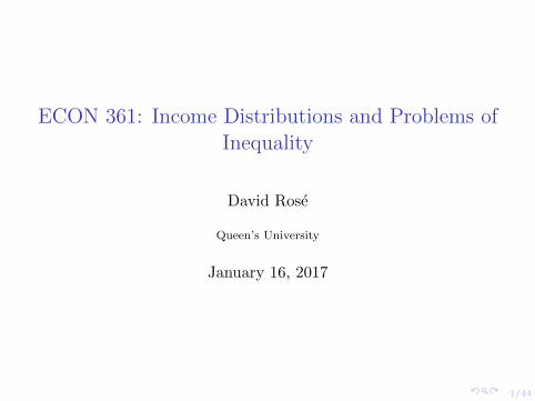
Fundamental Concepts

I Population: includes all members of the group we are studying orcollecting info about

I Sample: A subset of the population

Since observing the population is often impossible (or prohibitivelyexpensive), we study samples to learn about the population.

5/44

Example: Suppose we’re interested in studying the IQ of Canadians.

We randomly sample from the population of Canada and administer IQtests ... now what?

Question: How can we summarize the data to make learning about itmanageable?

Two types of measures that are useful:

1. Measures of central tendency: trying to come up with a“typical” data point

2. Measures of dispersion: trying to capture how spread out theobservations are

6/44

measures of central tendency

sample mean (a.k.a. the sample average):

x =1

n

n∑i=1

xi

median: obtained by ordering each of the n observations from smallestto largest value and then the median is:

x =

(n+ 1

2

)thordered value if n is odd

and

x = average of(n

2

)thand

(n+ 1

2

)thordered values if n is even

7/44

Example: MCT

8/44

Measures of Dispersion:

Range: The difference between the highest observation and lowestobservations

Interquartile range: The difference between the 75th and 25thpercentile (excludes obs. in the tails)

Sample variance: captures the average squared distance ofobservations from the sample mean

s2 =1

N − 1

N∑i=1

(xi − x)2

9/44

Example: Measures of Dispersion

10/44

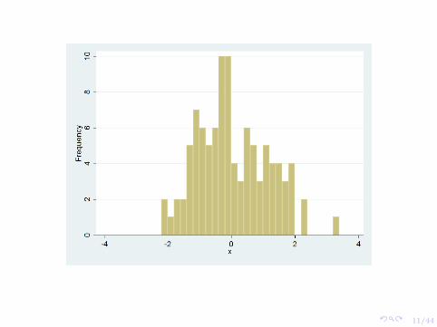
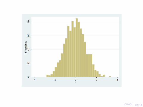
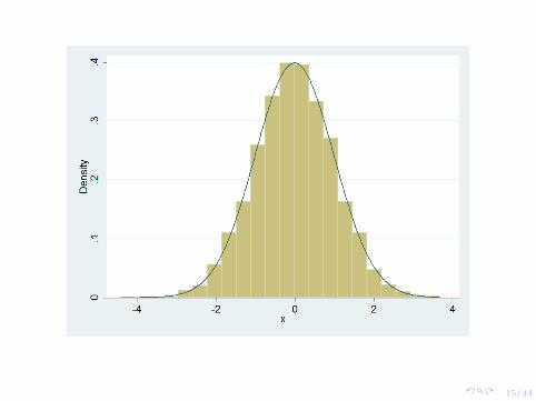
Frequency distribution: think histogram!

Each bin represents an interval of the random variable (say X) and thefrequency with which X falls in the given interval.

Next slides are frequency distributions for 100 and 1000 observationsthat are normally distributed with mean 0 and variance 1.

The frequency distribution then groups all values in to bins and tells usthe number of values observed in each bin.

14/44

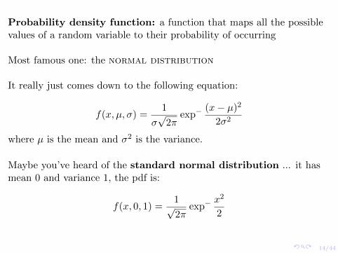
Probability density function: a function that maps all the possiblevalues of a random variable to their probability of occurring

Most famous one: the normal distribution

It really just comes down to the following equation:

f(x, µ, σ) =1

σ√

2πexp−

(x− µ)2

2σ2

where µ is the mean and σ2 is the variance.

Maybe you’ve heard of the standard normal distribution ... it hasmean 0 and variance 1, the pdf is:

f(x, 0, 1) =1√2π

exp−x2

2

16/44

This is an example of a probability distribution: (f(x) = P (X = x))

I the probability distribution is very similar to the frequencydistribution

I the y axis tells us the probability that an observation falls within acertain bin.

Question: how do you think the probabilities are related to thefrequency?

I probability = (# of obs in a bin) / (# obs in the sample)

17/44

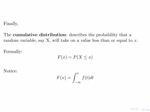
Finally,

The cumulative distribution: describes the probability that arandom variable, say X, will take on a value less than or equal to x.

Formally:F (x) = P (X ≤ x)

Notice:

F (x) =

∫ x

−∞f(t)dt

19/44

Some notes on distributions:

I The distribution is symmetric if the left half is a mirror image ofthe right half

I A positive skewness occurs when the right half of thedistribution is stretched out (compared with the left)

I A negative skewness occurs when the left half of the distributionis stretched out (compared with the right)

I The kurtosis captures the amount of ‘stretching’ in thedistribution. More formally, it indicates the amount of mass in thetails of the distribution.

20/44

Frequency distribution of Canadian After-Tax Income (from 2006Census PUMF):

21/44

Probability distribution of Canadian After-Tax Income (from 2006Census PUMF):

22/44

Cumulative distribution of Canadian After-Tax Income:

23/44

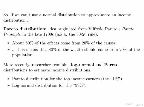
So, if we can’t use a normal distribution to approximate an incomedistribution ...

Pareto distribution: idea originated from Vilfredo Pareto’s ParetoPrinciple in the late 1700s (a.k.a. the 80-20 rule).

I About 80% of the effects come from 20% of the causes.

I ... this means that 80% of the wealth should come from 20% of thepopulation.

More recently, researchers combine log-normal and Paretodistributions to estimate income distributions.

I Pareto distribution for the top income earners (the “1%”)

I Log-normal distribution for the “99%”.

24/44

0 10 20 30 40 50

0.0

0.2

0.4

x

dpar

eto(

x)

25/44

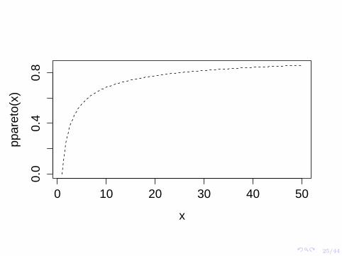
0 10 20 30 40 50

0.0

0.4

0.8

x

ppar

eto(

x)

26/44

Hypothesis testing: The Ontario Avg. Wage

I Suppose you are told that average earnings in Ontario are$20.00/hour.

I You collect data from a sample of individuals and calculate themean of your sample to be $22.46 (i.e. Y ).

I Given our data, we might question whether the population meanreally is $20.00 ...

How do we go about formulating this in a meaningful hypothesis test?

27/44

Null hypothesis: “The population mean wage is $20/hrHo: µY = 20

Alternative hypothesis: : “The population mean wage is not $20/hrHa: µY 6= 20

I This is known as a two-sided test because our alternativehypothesis contains both the possibility that µY > 20 and µY < 20.

We either reject Ho or fail to reject Ho, but in general we do not saythat we accept Ho.

28/44

Central limit theorem Y ∼ N (µY , σ2Y

).

z-statistic: a way to “standardize” Y :

I Z =∣∣∣ Y−µYσY

∣∣∣ and Z ∼ N (0, 1)

I When σY is unknown we calculate the t-statistic. It’s very similarto the z-statistic except it uses S.E.(Y ) which is close to σY inlarge samples.

I t =∣∣∣ Y−µYS.E.(Y )

∣∣∣ and t ∼ N (0, 1)

Rejection rule: We reject Ho if |tact| ≥ |t∗|

29/44

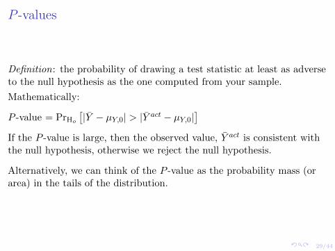
P -values

Definition: the probability of drawing a test statistic at least as adverseto the null hypothesis as the one computed from your sample.

Mathematically:

P -value = PrHo

[|Y − µY,0| > |Y act − µY,0|

]If the P -value is large, then the observed value, Y act is consistent withthe null hypothesis, otherwise we reject the null hypothesis.

Alternatively, we can think of the P -value as the probability mass (orarea) in the tails of the distribution.

31/44

P-Values: The Intuition

A p-value answers the question:

I If our null hypothesis (H0) is correct, what’s the probability thatwe would observe a particular sample statistic in our sample?’

Back to our avg. wage example:

I We calculate Y = $22.46 in our sample

I The null hypothesis is that µY = $20.00 ... clearly these aredifferent numbers

I But what’s the probability that this difference in the two numbersis just caused by randomness?

32/44

Confidence Intervals:

Due to random error we can’t recover the true population parameter(for example the mean, µ) using only sample information.

But we can use information from our sample to come up with a set ofvalues that contains µ with some specified probability.

I We’re using sample statistics to say something meaningful aboutthe true parameters.

33/44

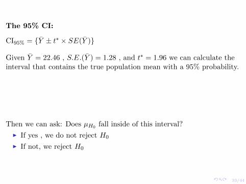
The 95% CI:

CI95% = {Y ± t∗ × SE(Y )}

Given Y = 22.46 , S.E.(Y ) = 1.28 , and t∗ = 1.96 we can calculate theinterval that contains the true population mean with a 95% probability.

Then we can ask: Does µH0 fall inside of this interval?

I If yes , we do not reject H0

I If not, we reject H0

34/44

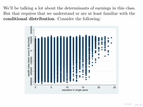
We’ll be talking a lot about the determinants of earnings in this class.But that requires that we understand or are at least familiar with theconditional distribution. Consider the following:

-300

000

-200

000

-100

000

010

0000

2000

00w

ealth

inde

x fa

ctor

sco

re (5

dec

imal

s)

0 5 10 15 20 25education in single years

35/44

01.

0e-0

62.0

e-06

3.0e

-064

.0e-

06D

ensi

ty

-300000 -200000 -100000 0 100000wealth index factor score (5 decimals)

02.

0e-0

64.

0e-0

66.

0e-0

6D

ensi

ty


02.

0e-0

64.0e

-066.0e

-068.0e

-061.0e

-05

Den

sity


05.

0e-0

61.

0e-0

51.

5e-0

5D

ensi

ty


36/44

The conditional distribution describes the distribution of a randomvariable, Y , conditional on the variable, X, taking on a given value:

Pr(Y = y|X = x) =Pr(X = x, Y = y)

Pr(X = x)

Other important formulae:

I Covariance:

Cov(x, y) =1

N

N∑i=1

(xi − x)(yi − y)

I If x and y are uncorrelated, the covariance is 0.I If x increases and y increases, the covariance is positive.I If x increases and y decreases, the covariance is negative.

37/44

Another linear measure of correlation that is bounded between -1 and 1is the correlation coefficient:

ρ =Cov(x, y)√

Var(x)√

Var(y)

38/44

-500

000

5000

010

0000

1500

00(m

ean)

hv2

71


39/44

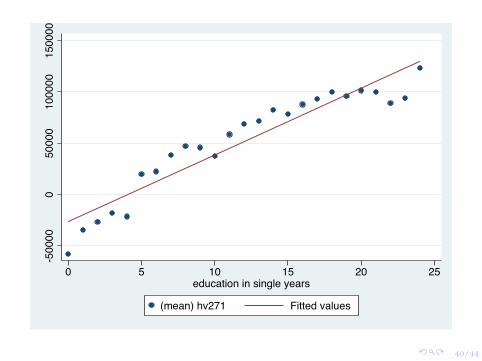
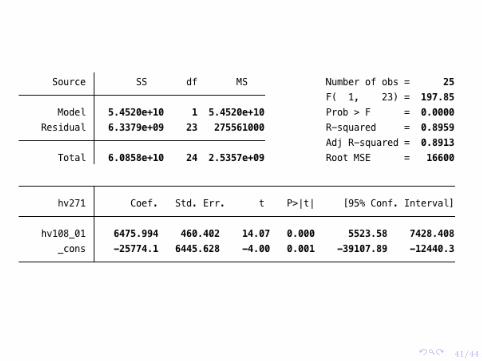
So how would an economist estimate a relationship between educationand income (or in this case, the wealth index)?

The linear regression model postulates just that - a linear relationshipbetween two (or more) variables.

Yi = β0 + β1Xi + εi

Where, β0 is the intercept, β1 is the slope, Yi is the dependent variable,Xi is the independent variable and εi is an error component.

The parameters (β0 and β1 are chosen such that the sum of squaredresiduals are minimized.

40/44

-500

000

5000

010

0000

1500

00


(mean) hv271 Fitted values

42/44

420 QUARTERLY JOURNAL OF ECONOMICS

and I/GDP is 0.59 for the intermediate sample, and the correlation between SCHOOL and the population growth rate is -0.38. Thus, including human-capital accumulation could alter substantially the estimated impact of physical-capital accumulation and population growth on income per capita.

C. Results Table II presents regressions of the log of income per capita on

the log of the investment rate, the log of n + g + 8, and the log of the percentage of the population in secondary school. The human- capital measure enters significantly in all three samples. It also

TABLE II ESTIMATION OF THE AUGMENTED SOLOW MODEL

Dependent variable: log GDP per working-age person in 1985

Sample: Non-oil Intermediate OECD Observations: 98 75 22 CONSTANT 6.89 7.81 8.63

(1.17) (1.19) (2.19) ln(I/GDP) 0.69 0.70 0.28

(0.13) (0.15) (0.39) ln(n + g + 5) -1.73 -1.50 -1.07

(0.41) (0.40) (0.75) ln(SCHOOL) 0.66 0.73 0.76

(0.07) (0.10) (0.29) R2 0.78 0.77 0.24 s.e.e. 0.51 0.45 0.33 Restricted regression: CONSTANT 7.86 7.97 8.71

(0.14) (0.15) (0.47) ln(I/GDP) - ln(n + g + 5) 0.73 0.71 0.29

(0.12) (0.14) (0.33) ln(SCHOOL) - ln(n + g + 5) 0.67 0.74 0.76

(0.07) (0.09) (0.28) R2 0.78 0.77 0.28 s.e.e. 0.51 0.45 0.32 Test of restriction:

p-value 0.41 0.89 0.97 Implied a 0.31 0.29 0.14

(0.04) (0.05) (0.15) Implied , 0.28 0.30 0.37

(0.03) (0.04) (0.12)

Note. Standard errors are in parentheses. The investment and population growth rates are averages for the period 1960-1985. (g + 8) is assumed to be 0.05. SCHOOL is the average percentage of the working-age population in secondary school for the period 1960-1985.

This content downloaded from 130.15.32.38 on Mon, 15 Sep 2014 12:21:17 PMAll use subject to JSTOR Terms and Conditions

420 QUARTERLY JOURNAL OF ECONOMICS

and I/GDP is 0.59 for the intermediate sample, and the correlation between SCHOOL and the population growth rate is -0.38. Thus, including human-capital accumulation could alter substantially the estimated impact of physical-capital accumulation and population growth on income per capita.

C. Results Table II presents regressions of the log of income per capita on

the log of the investment rate, the log of n + g + 8, and the log of the percentage of the population in secondary school. The human- capital measure enters significantly in all three samples. It also

TABLE II ESTIMATION OF THE AUGMENTED SOLOW MODEL

Dependent variable: log GDP per working-age person in 1985

Sample: Non-oil Intermediate OECD Observations: 98 75 22 CONSTANT 6.89 7.81 8.63

(1.17) (1.19) (2.19) ln(I/GDP) 0.69 0.70 0.28

(0.13) (0.15) (0.39) ln(n + g + 5) -1.73 -1.50 -1.07

(0.41) (0.40) (0.75) ln(SCHOOL) 0.66 0.73 0.76

(0.07) (0.10) (0.29) R2 0.78 0.77 0.24 s.e.e. 0.51 0.45 0.33 Restricted regression: CONSTANT 7.86 7.97 8.71

(0.14) (0.15) (0.47) ln(I/GDP) - ln(n + g + 5) 0.73 0.71 0.29

(0.12) (0.14) (0.33) ln(SCHOOL) - ln(n + g + 5) 0.67 0.74 0.76

(0.07) (0.09) (0.28) R2 0.78 0.77 0.28 s.e.e. 0.51 0.45 0.32 Test of restriction:

p-value 0.41 0.89 0.97 Implied a 0.31 0.29 0.14

(0.04) (0.05) (0.15) Implied , 0.28 0.30 0.37

(0.03) (0.04) (0.12)

Note. Standard errors are in parentheses. The investment and population growth rates are averages for the period 1960-1985. (g + 8) is assumed to be 0.05. SCHOOL is the average percentage of the working-age population in secondary school for the period 1960-1985.

This content downloaded from 130.15.32.38 on Mon, 15 Sep 2014 12:21:17 PMAll use subject to JSTOR Terms and Conditions

43/44

Some notes:

I Pay attention to the magnitude of the coefficient estimates.

I Note if the regression is in log form and also note how it isestimated: probit, logit, tobit, etc.

I P -values, t statistics, standard errors, clustering, bootstrap (whatvalues are listed in parentheses).

I R2 measures goodness of fit, it tells us the fraction of the variancein Y explained by the variance in X.

44/44

Next class, “papers in poverty measurement”, readings:

1. Osberg, Lars and Kuan Xu (1999). Poverty Intensity: How Well DoCanadian Provinces Compare? Canadian Public Policy, 25(2),179-195.

2. Osberg, Lars (2000). Poverty in Canada and the United States:Measurement, Trends, and Implications. The Canadian Journal ofEconomics, 33(4), 847-877.

3. Chen, Shaohua and Martin Ravallion (2010). The DevelopingWorld is Poorer Than We Thought, but No Less Successful in theFight Against Poverty. The Quarterly Journal of Economics,124(4), 1577-1625.

ECON 361: Income Distributions and Problems of Inequality · · 2017-01-17ECON 361: Income...

Documents

Transcript of ECON 361: Income Distributions and Problems of Inequality · · 2017-01-17ECON 361: Income...