The Econ Exchange The Econ Exchange - Department of Economics

ECON 337901
FINANCIAL ECONOMICS
Peter Ireland
Boston College
Spring 2018
These lecture notes by Peter Ireland are licensed under a Creative Commons Attribution-NonCommerical-ShareAlike4.0 International (CC BY-NC-SA 4.0) License. http://creativecommons.org/licenses/by-nc-sa/4.0/.
3 Making Choices in Risky Situations
A Criteria for Choice Over Risky Prospects
B Preferences and Utility Functions
C Expected Utility Functions
D The Expected Utility Theorem
E The Allais Paradox
F Generalizations of Expected Utility
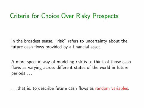
Criteria for Choice Over Risky Prospects
In the broadest sense, “risk” refers to uncertainty about thefuture cash flows provided by a financial asset.
A more specific way of modeling risk is to think of those cashflows as varying across different states of the world in futureperiods . . .
. . . that is, to describe future cash flows as random variables.
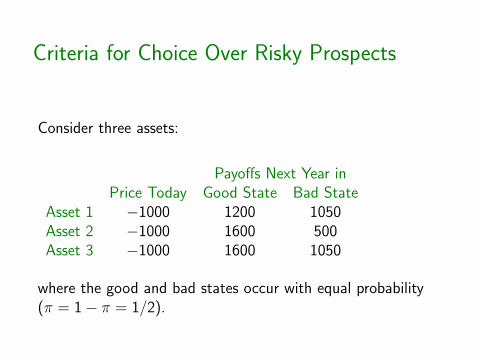
Criteria for Choice Over Risky Prospects
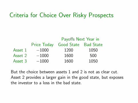
Consider three assets:
Payoffs Next Year inPrice Today Good State Bad State
Asset 1 −1000 1200 1050Asset 2 −1000 1600 500Asset 3 −1000 1600 1050
where the good and bad states occur with equal probability(π = 1− π = 1/2).
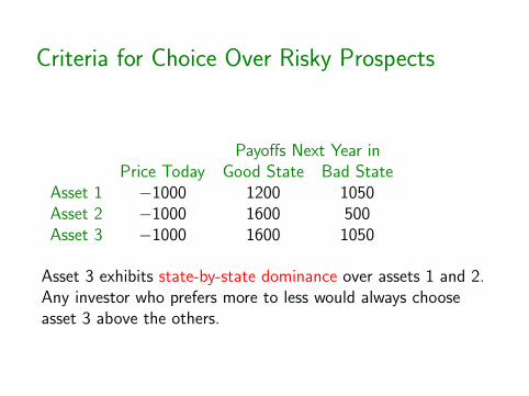
Criteria for Choice Over Risky Prospects
Payoffs Next Year inPrice Today Good State Bad State
Asset 1 −1000 1200 1050Asset 2 −1000 1600 500Asset 3 −1000 1600 1050
Asset 3 exhibits state-by-state dominance over assets 1 and 2.Any investor who prefers more to less would always chooseasset 3 above the others.
Criteria for Choice Over Risky Prospects
Payoffs Next Year inPrice Today Good State Bad State
Asset 1 −1000 1200 1050Asset 2 −1000 1600 500Asset 3 −1000 1600 1050
But the choice between assets 1 and 2 is not as clear cut.Asset 2 provides a larger gain in the good state, but exposesthe investor to a loss in the bad state.
Criteria for Choice Over Risky Prospects
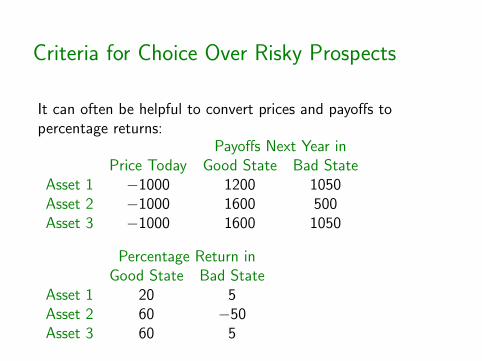
It can often be helpful to convert prices and payoffs topercentage returns:
Payoffs Next Year inPrice Today Good State Bad State
Asset 1 −1000 1200 1050Asset 2 −1000 1600 500Asset 3 −1000 1600 1050
Percentage Return inGood State Bad State
Asset 1 20 5Asset 2 60 −50Asset 3 60 5

Criteria for Choice Over Risky Prospects
In probability theory, if a random variable X can take on npossible values, X1,X2, . . . ,Xn, with probabilitiesπ1, π2, . . . , πn, then the expected value of X is
E (X ) = π1X1 + π2X2 + . . . + πnXn,
the variance of X is
σ2(X ) = π1[X1 − E (X )]2
+π2[X2 − E (X )]2 + . . . + πn[Xn − E (X )]2,
and the standard deviation of X is σ(X ) = [σ2(X )]1/2.
Criteria for Choice Over Risky Prospects
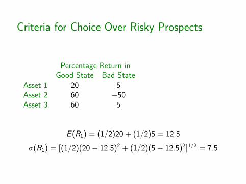
Percentage Return inGood State Bad State
Asset 1 20 5Asset 2 60 −50Asset 3 60 5
E (R1) = (1/2)20 + (1/2)5 = 12.5
σ(R1) = [(1/2)(20− 12.5)2 + (1/2)(5− 12.5)2]1/2 = 7.5

Criteria for Choice Over Risky Prospects
Percentage Return inGood State Bad State E (R) σ(R)
Asset 1 20 5 12.5 7.5Asset 2 60 −50Asset 3 60 5
E (R2) = (1/2)60 + (1/2)(−50) = 5
σ(R2) = [(1/2)(60− 5)2 + (1/2)(−50− 5)2]1/2 = 55

Criteria for Choice Over Risky Prospects
Percentage Return inGood State Bad State E (R) σ(R)
Asset 1 20 5 12.5 7.5Asset 2 60 −50 5 55Asset 3 60 5
E (R3) = (1/2)60 + (1/2)5 = 32.5
σ(R3) = [(1/2)(60− 32.5)2 + (1/2)(5− 32.5)2]1/2 = 27.5
Criteria for Choice Over Risky Prospects
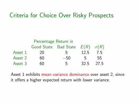
Percentage Return inGood State Bad State E (R) σ(R)
Asset 1 20 5 12.5 7.5Asset 2 60 −50 5 55Asset 3 60 5 32.5 27.5
Asset 1 exhibits mean-variance dominance over asset 2, sinceit offers a higher expected return with lower variance.

Criteria for Choice Over Risky Prospects
Percentage Return inGood State Bad State E (R) σ(R)
Asset 1 20 5 12.5 7.5Asset 2 60 −50 5 55Asset 3 60 5 32.5 27.5
But notice that by the mean-variance criterion, asset 3dominates asset 2 but not asset 1, even though on astate-by-state basis, asset 3 is clearly to be preferred.

Criteria for Choice Over Risky Prospects
Consider two more assets:
Percentage Return inGood State Bad State E (R) σ(R)
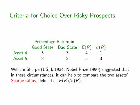
Asset 4 5 3Asset 5 8 2
Again, neither exhibits state-by-state dominance, so let’s tryto use the mean-variance criterion again.

Criteria for Choice Over Risky Prospects
Percentage Return inGood State Bad State E (R) σ(R)
Asset 4 5 3Asset 5 8 2
E (R4) = (1/2)5 + (1/2)3 = 4
σ(R4) = [(1/2)(5− 4)2 + (1/2)(3− 4)2]1/2 = 1
E (R5) = (1/2)8 + (1/2)2 = 5
σ(R5) = [(1/2)(8− 5)2 + (1/2)(2− 5)2]1/2 = 3

Criteria for Choice Over Risky Prospects
Percentage Return inGood State Bad State E (R) σ(R)
Asset 4 5 3 4 1Asset 5 8 2 5 3
Neither asset exhibits mean-variance dominance either.
Criteria for Choice Over Risky Prospects
Percentage Return inGood State Bad State E (R) σ(R)
Asset 4 5 3 4 1Asset 5 8 2 5 3
William Sharpe (US, b.1934, Nobel Prize 1990) suggested thatin these circumstances, it can help to compare the two assets’Sharpe ratios, defined as E (R)/σ(R).

Criteria for Choice Over Risky Prospects
Percentage Return inGood State Bad State E (R) σ(R) E/σ
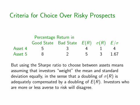
Asset 4 5 3 4 1 4Asset 5 8 2 5 3 1.67
Comparing Sharpe ratios, asset 4 is preferred to asset 5.
Criteria for Choice Over Risky Prospects
Percentage Return inGood State Bad State E (R) σ(R) E/σ
Asset 4 5 3 4 1 4Asset 5 8 2 5 3 1.67
But using the Sharpe ratio to choose between assets meansassuming that investors “weight” the mean and standarddeviation equally, in the sense that a doubling of σ(R) isadequately compensated by a doubling of E (R). Investors whoare more or less averse to risk will disagree.
Criteria for Choice Over Risky Prospects
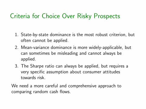
1. State-by-state dominance is the most robust criterion, butoften cannot be applied.
2. Mean-variance dominance is more widely-applicable, butcan sometimes be misleading and cannot always beapplied.
3. The Sharpe ratio can always be applied, but requires avery specific assumption about consumer attitudestowards risk.
We need a more careful and comprehensive approach tocomparing random cash flows.

Preferences and Utility Functions
Of course, economists face a more general problem of thiskind.
Even if we accept that more (of everything) is preferred toless, how do consumers compare different “bundles” of goodsthat may contain more of one good but less of another?
Microeconomists have identified a set of conditions that allowa consumer’s preferences to be described by a utility function.
Preferences and Utility Functions
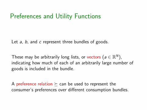
Let a, b, and c represent three bundles of goods.
These may be arbitrarily long lists, or vectors (a ∈ RN),indicating how much of each of an arbitrarily large number ofgoods is included in the bundle.
A preference relation � can be used to represent theconsumer’s preferences over different consumption bundles.

Preferences and Utility Functions
The expressiona � b
indicates that the consumer strictly prefers a to b,
a ∼ b
indicates that the consumer is indifferent between a and b, and
a � b
indicates that the consumer either strictly prefers or isindifferent between a and b.

Preferences and Utility Functions
A1 The preference relation is assumed to be complete: Forany two bundles a and b, either a � b, b � a, or both, and inthe latter case a ∼ b.
The consumer has to decide whether he or she prefers onebundle to another or is indifferent between the two.Ambiguous tastes are not allowed.
Preferences and Utility Functions
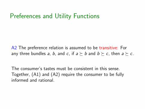
A2 The preference relation is assumed to be transitive: Forany three bundles a, b, and c , if a � b and b � c , then a � c .
The consumer’s tastes must be consistent in this sense.Together, (A1) and (A2) require the consumer to be fullyinformed and rational.
Preferences and Utility Functions
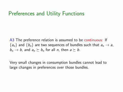
A3 The preference relation is assumed to be continuous: If{an} and {bn} are two sequences of bundles such that an → a,bn → b, and an � bn for all n, then a � b.
Very small changes in consumption bundles cannot lead tolarge changes in preferences over those bundles.
Preferences and Utility Functions
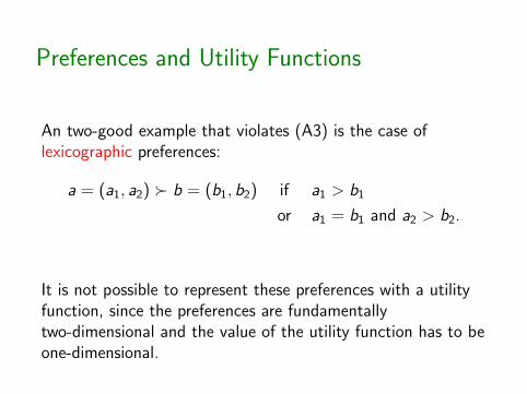
An two-good example that violates (A3) is the case oflexicographic preferences:
a = (a1, a2) � b = (b1, b2) if a1 > b1
or a1 = b1 and a2 > b2.
It is not possible to represent these preferences with a utilityfunction, since the preferences are fundamentallytwo-dimensional and the value of the utility function has to beone-dimensional.

Preferences and Utility Functions
The following theorem was proven by Gerard Debreu in 1954.
Theorem If preferences are complete, transitive, andcontinuous, then they can be represented by a continuous,real-valued utility function. That is, if (A1)-(A3) hold, there isa continuous function u : Rn 7→ R such that for any twoconsumption bundles a and b,
a � b if and only if u(a) ≥ u(b).

Preferences and Utility Functions
Note that if preferences are represented by the utility functionu,
a � b if and only if u(a) ≥ u(b),
then they are also represented by the utility function v , where
v(a) = F (u(a))
and F : R 7→ R is any increasing function.
The concept of utility as it is used in standard microeconomictheory is ordinal, as opposed to cardinal.
Expected Utility Functions
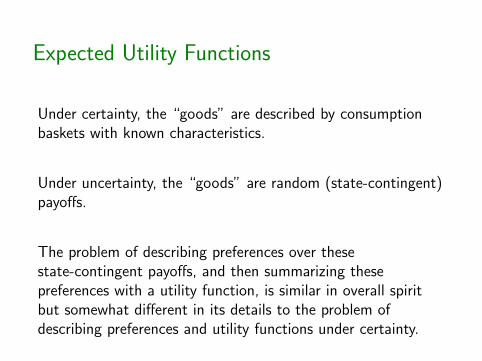
Under certainty, the “goods” are described by consumptionbaskets with known characteristics.
Under uncertainty, the “goods” are random (state-contingent)payoffs.
The problem of describing preferences over thesestate-contingent payoffs, and then summarizing thesepreferences with a utility function, is similar in overall spiritbut somewhat different in its details to the problem ofdescribing preferences and utility functions under certainty.
Expected Utility Functions
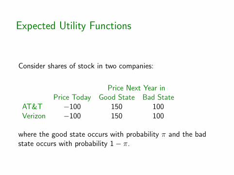
Consider shares of stock in two companies:
Price Next Year inPrice Today Good State Bad State
AT&T −100 150 100Verizon −100 150 100
where the good state occurs with probability π and the badstate occurs with probability 1− π.

Expected Utility Functions
Price Next Year inPrice Today Good State Bad State
AT&T −100 150 100Verizon −100 150 100
probability π 1− π
We will assume that if the two assets provide exactly the samestate-contingent payoffs, then investors will be indifferentbetween them.

Expected Utility Functions
Price Next Year inPrice Today Good State Bad State
AT&T −100 150 100Verizon −100 150 100
probability π 1− π
1. Investors care only about payoffs and probabilities.
Expected Utility Functions
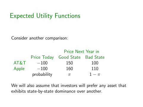
Consider another comparison:
Price Next Year inPrice Today Good State Bad State
AT&T −100 150 100Apple −100 160 110
probability π 1− π
We will also assume that investors will prefer any asset thatexhibits state-by-state dominance over another.

Expected Utility Functions
Price Next Year inPrice Today Good State Bad State
AT&T −100 150 100Apple −100 160 110
probability π 1− π
2. If u(p) measures utility from the payoff p in any particularstate, then u is increasing.
Expected Utility Functions
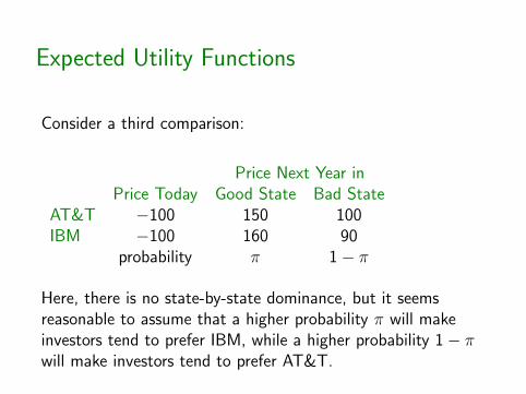
Consider a third comparison:
Price Next Year inPrice Today Good State Bad State
AT&T −100 150 100IBM −100 160 90
probability π 1− π
Here, there is no state-by-state dominance, but it seemsreasonable to assume that a higher probability π will makeinvestors tend to prefer IBM, while a higher probability 1− πwill make investors tend to prefer AT&T.

Expected Utility Functions
Price Next Year inPrice Today Good State Bad State
AT&T −100 150 100IBM −100 160 90
probability π 1− π
3. Investors should care more about states of the world thatoccur with greater probability.

Expected Utility Functions
A criterion that has all three of these properties was suggestedby Blaise Pascal (France, 1623-1662): base decisions on theexpected payoff,
E (p) = πpG + (1− π)pB ,
where pG and pB , with pG > pB , are the payoffs in the goodand bad states.
Expected Utility Functions
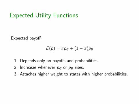
Expected payoff
E (p) = πpG + (1− π)pB
1. Depends only on payoffs and probabilities.
2. Increases whenever pG or pB rises.
3. Attaches higher weight to states with higher probabilities.

Expected Utility Functions
Nicolaus Bernoulli (Switzerland, 1687-1759) pointed to aproblem with basing investment decisions exclusively onexpected payoffs: it ignores risk. To see this, specialize theprevious example by setting π = 1− π = 1/2 but add, as well,a third asset:
Price Next Year inPrice Today Good State Bad State
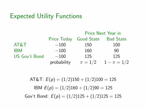
AT&T −100 150 100IBM −100 160 90US Gov’t Bond −100 125 125
probability π = 1/2 1− π = 1/2
Expected Utility Functions
Price Next Year inPrice Today Good State Bad State
AT&T −100 150 100IBM −100 160 90US Gov’t Bond −100 125 125
probability π = 1/2 1− π = 1/2
AT&T: E (p) = (1/2)150 + (1/2)100 = 125
IBM E (p) = (1/2)160 + (1/2)90 = 125
Gov’t Bond: E (p) = (1/2)125 + (1/2)125 = 125
Expected Utility Functions
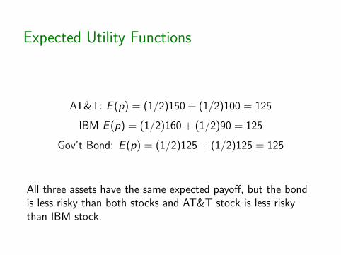
AT&T: E (p) = (1/2)150 + (1/2)100 = 125
IBM E (p) = (1/2)160 + (1/2)90 = 125
Gov’t Bond: E (p) = (1/2)125 + (1/2)125 = 125
All three assets have the same expected payoff, but the bondis less risky than both stocks and AT&T stock is less riskythan IBM stock.
Expected Utility Functions
Gabriel Cramer (Switzerland, 1704-1752) and Daniel Bernoulli(Switzerland, 1700-1782) suggested that more reliablecomparisons could be made by assuming that the utilityfunction u over payoffs in any given state is concave as well asincreasing.
This implies that investors prefer more to less, but havediminishing marginal utility as payoffs increase.
Expected Utility Functions
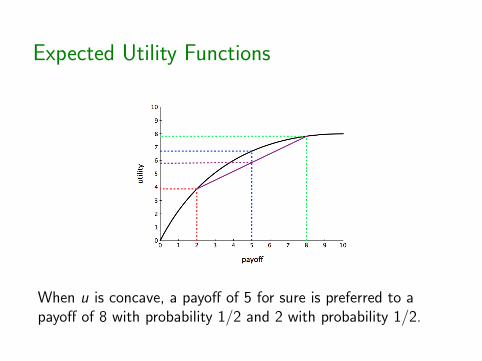
When u is concave, a payoff of 5 for sure is preferred to apayoff of 8 with probability 1/2 and 2 with probability 1/2.

Expected Utility Functions
About two centuries later, John von Neumann (Hungary,1903-1957) and Oskar Morgenstern (Germany, 1902-1977)worked out the conditions under which investors’ preferencesover risky payoffs could be described by an expected utilityfunction such as
U(p) = E [u(p)] = πu(pG ) + (1− π)u(pB),
where the Bernoulli utility function over payoffs u is increasingand concave and the von Neumann-Morgenstern expectedutility function U is linear in the probabilities.

Expected Utility Functions
von Neumann and Morgenstern’s axiomatic derivation ofexpected utility appeared in the second edition of their book,Theory of Games and Economic Behavior, published in 1947.
U(p) = E [u(p)] = πu(pG ) + (1− π)u(pB)
Linearity in the probabilities is the “defining characteristic” ofthe expected utility function U(p).

The Expected Utility Theorem
The simple lottery (x , y , π) offers payoff x with probability πand payoff y with probability 1− π.
The Expected Utility Theorem
The simple lottery (x , y , π) offers payoff x with probability πand payoff y with probability 1− π.
In this definition, x and y can be monetary payoffs, as in thestock and bond examples from before.
Alternatively, they can be additional lotteries!
The Expected Utility Theorem
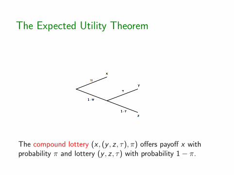
The compound lottery (x , (y , z , τ), π) offers payoff x withprobability π and lottery (y , z , τ) with probability 1− π.

The Expected Utility Theorem
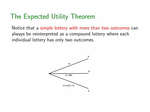
Notice that a simple lottery with more than two outcomes canalways be reinterpreted as a compound lottery where eachindividual lottery has only two outcomes.
The Expected Utility Theorem
Notice that a simple lottery with more than two outcomes canalways be reinterpreted as a compound lottery where eachindividual lottery has only two outcomes.

The Expected Utility Theorem
Notice that a simple lottery with more than two outcomes canalways be reinterpreted as a compound lottery where eachindividual lottery has only two outcomes.
The Expected Utility Theorem
Notice that a simple lottery with more than two outcomes canalways be reinterpreted as a compound lottery where eachindividual lottery has only two outcomes.
So restricting ourselves to lotteries with only two outcomesdoes not entail any loss of generality in terms of the numberof future states that are possible.
But to begin describing preferences over lotteries, we need tomake additional assumptions.

The Expected Utility Theorem
B1a A lottery that pays off x with probability one is the sameas getting x for sure: (x , y , 1) = x .
B1b Investors care about payoffs and probabilities, but not thespecific ordering of the states: (x , y , π) = (y , x , 1− π)
B1c In evaluating compound lotteries, investors care onlyabout the probabilities of each final payoff:(x , z , π) = (x , y , π + (1− π)τ) if z = (x , y , τ).

The Expected Utility Theorem
B2 There exists a preference relation � defined on lotteriesthat is complete and transitive.
Again, this amounts to requiring that investors are fullyinformed and rational.
The Expected Utility Theorem
B3 The preference relation � defined on lotteries iscontinuous.
Hence, very small changes in lotteries cannot lead to very largechanges in preferences over those lotteries.
The Expected Utility Theorem
By the previous theorem, we already know that (B2) and (B3)are sufficient to guarantee the existence of a utility functionover lotteries and, by (B1a), payoffs received with certainty aswell.
What remains is to identify the extra assumptions thatguarantee that this utility function is linear in the probabilies,that is, of the von Neumann-Morgenstern (vN-M) form.
The Expected Utility Theorem
B4 Independence axiom: For any two lotteries (x , y , π) and(x , z , π), y � z if and only if (x , y , π) � (x , z , π).
This assumption is controversial and unlike any made intraditional microeconomic theory: you would not necessarywant to assume that a consumer’s preferences oversub-bundles of any two goods are independent of how much ofa third good gets included in the overall bundle. But it isneeded for the utility function to take the vN-M form.

The Expected Utility Theorem
There is a technical assumption that makes the expectedutility theorem easier to prove.
B5 There is a best lottery b and a worst lottery w .
This assumption will automatically hold if there are only afinite number of possible payoffs and if the independenceaxiom holds.

The Expected Utility Theorem
Finally, there are two additional assumptions that, strictlyspeaking, follow from those made already:
B6 (implied by (B3)) Let x , y , and z satisfy x � y � z . Thenthere exists a probability π such that (x , z , π) ∼ y .
B7 (implied by (B4)) Let x � y . Then (x , y , π1) � (x , y , π2) ifand only if π1 > π2.
The Expected Utility Theorem
Theorem (Expected Utility Theorem) If (B1)-(B7) hold, thenthere exists a utility function U defined over lotteries such that
U((x , y , π)) = πu(x) + (1− π)u(y).
Note that we can prove the theorem simply by “constructing”the utility functions U and u with the desired properties.

The Expected Utility Theorem
Begin by settingU(b) = 1
U(w) = 0.
For any lottery z besides the best and worst, (B6) implies thatthere exists a probability πz such that (b,w , πz) ∼ z and (B7)implies that this probability is unique. For this lottery, set
U(z) = πz .
The Expected Utility Theorem
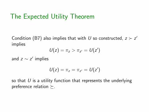
Condition (B7) also implies that with U so constructed, z � z ′
impliesU(z) = πz > πz ′ = U(z ′)
and z ∼ z ′ implies
U(z) = πz = πz ′ = U(z ′)
so that U is a utility function that represents the underlyingpreference relation �.
The Expected Utility Theorem
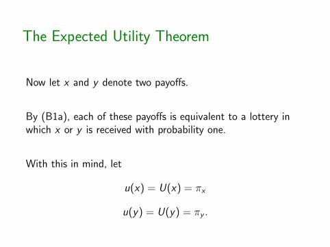
Now let x and y denote two payoffs.
By (B1a), each of these payoffs is equivalent to a lottery inwhich x or y is received with probability one.
With this in mind, let
u(x) = U(x) = πx
u(y) = U(y) = πy .

The Expected Utility Theorem
Finally, let π denote a probability and consider the lotteryz = (x , y , π).
Condition (B1c) implies
(x , y , π) ∼ ((b,w , πx), (b,w , πy ), π) ∼ (b,w , ππx + (1−π)πy )
But this last expression is equivalent to
U(z) = U(x , y , π) = ππx + (1− π)πy = πu(x) + (1− π)u(y),
confirming that U has the vN-M form.

The Expected Utility Theorem
Note that the key property of the vN-M utility function
U(z) = U(x , y , π) = πu(x) + (1− π)u(y),
its linearity in the probabilities π and 1− π, is not preservedby all transformations of the form
V (z) = F (U(z)),
where F is an increasing function.
In this sense, vN-M utility functions are cardinal, not ordinal.

The Expected Utility Theorem
On the other hand, given a vN-M utility function
U(z) = U(x , y , π) = πu(x) + (1− π)u(y),
consider an affine transformation
V (z) = αU(z) + β
and define
v(x) = αu(x) + β and v(y) = αu(y) + β
The Expected Utility Theorem
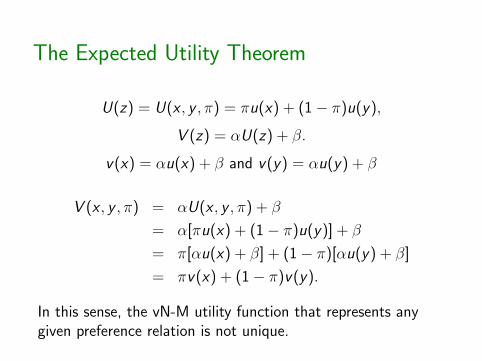
U(z) = U(x , y , π) = πu(x) + (1− π)u(y),
V (z) = αU(z) + β.
v(x) = αu(x) + β and v(y) = αu(y) + β
V (x , y , π) = αU(x , y , π) + β
= α[πu(x) + (1− π)u(y)] + β
= π[αu(x) + β] + (1− π)[αu(y) + β]
= πv(x) + (1− π)v(y).
In this sense, the vN-M utility function that represents anygiven preference relation is not unique.
The Allais Paradox
As mentioned previously, the independence axiom has beenand continues to be a subject of controversy and debate.
Maurice Allais (France, 1911-2010, Nobel Prize 1988)constructed a famous example that illustrates why theindependence axiom might not hold in his paper “LeComportement de L’Homme Rationnel Devant Le Risque:Critique Des Postulats et Axiomes De L’Ecole Americaine,”Econometrica Vol.21 (October 1953): pp.503-546.
The Allais Paradox
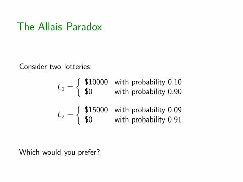
Consider two lotteries:
L1 =
{$10000 with probability 0.10$0 with probability 0.90
L2 =
{$15000 with probability 0.09$0 with probability 0.91
Which would you prefer?
The Allais Paradox
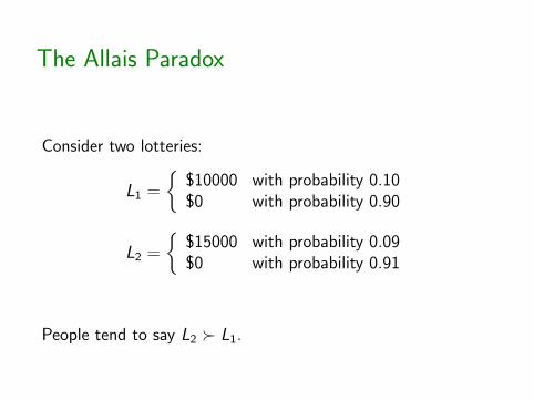
Consider two lotteries:
L1 =
{$10000 with probability 0.10$0 with probability 0.90
L2 =
{$15000 with probability 0.09$0 with probability 0.91
People tend to say L2 � L1.

The Allais Paradox
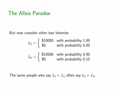
But now consider other two lotteries:
L3 =
{$10000 with probability 1.00$0 with probability 0.00
L4 =
{$15000 with probability 0.90$0 with probability 0.10
Which would you prefer?
The Allais Paradox
But now consider other two lotteries:
L3 =
{$10000 with probability 1.00$0 with probability 0.00
L4 =
{$15000 with probability 0.90$0 with probability 0.10
The same people who say L2 � L1 often say L3 � L4.
The Allais Paradox
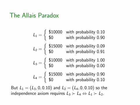
L1 =
{$10000 with probability 0.10$0 with probability 0.90
L2 =
{$15000 with probability 0.09$0 with probability 0.91
L3 =
{$10000 with probability 1.00$0 with probability 0.00
L4 =
{$15000 with probability 0.90$0 with probability 0.10
But L1 = (L3, 0, 0.10) and L2 = (L4, 0, 0.10) so theindependence axiom requires L3 � L4 ⇔ L1 � L2.

The Allais Paradox
L1 =
{$10000 with probability 0.10$0 with probability 0.90
L2 =
{$15000 with probability 0.09$0 with probability 0.91
L3 =
{$10000 with probability 1.00$0 with probability 0.00
L4 =
{$15000 with probability 0.90$0 with probability 0.10
The Allais paradox suggests that feelings about probabilitiesmay not always be “linear,” but linearity in the probabilities isprecisely what defines vN-M utility functions.

Generalizations of Expected Utility
Another potential limitation of expected utility is that it doesnot capture preferences for early or late resolution ofuncertainty.
A generalization of expected utility that makes this distinctionis proposed by David Kreps and Evan Porteus, “TemporalResolution of Uncertainty and Dynamic Choice Theory,”Econometrica Vol.46 (January 1978): pp.185-200.

Generalizations of Expected Utility
To model preferences for the temporal resolution ofuncertainty, consider two assets.
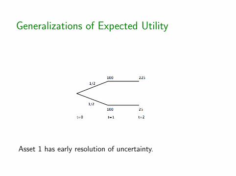
Both assets pay off $100 next year for sure. And both assetspay off $225 with probability 1/2 and $25 with probability 1/2two years from now.
But for asset 1, the payoff two years from now is revealed oneyear from now, whereas for asset 2, the payoff two years fromnow does not get revealed until the beginning of the secondyear.
Generalizations of Expected Utility
Asset 1 has early resolution of uncertainty.

Generalizations of Expected Utility
Asset 2 has late resolution of uncertainty.
Generalizations of Expected Utility
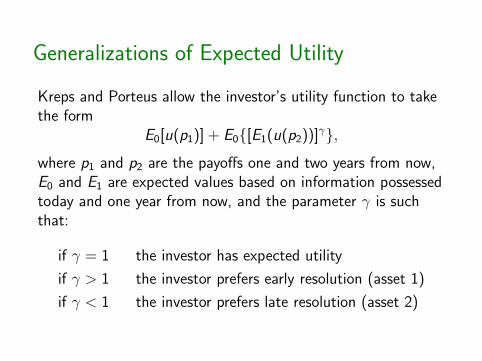
Kreps and Porteus allow the investor’s utility function to takethe form
E0[u(p1)] + E0{[E1(u(p2))]γ},
where p1 and p2 are the payoffs one and two years from now,E0 and E1 are expected values based on information possessedtoday and one year from now, and the parameter γ is suchthat:
if γ = 1 the investor has expected utility
if γ > 1 the investor prefers early resolution (asset 1)
if γ < 1 the investor prefers late resolution (asset 2)

Generalizations of Expected Utility
To see how this works, let
u(p) = p1/2
and call the state that leads to the 225 payoff two years fromnow the “good state” and the state that leads to the 25 payofftwo years from now the “bad state.”
Generalizations of Expected Utility
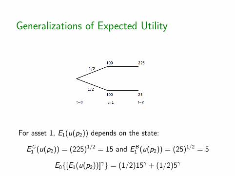
For asset 1, E1(u(p2)) depends on the state:
EG1 (u(p2)) = (225)1/2 = 15 and EB
1 (u(p2)) = (25)1/2 = 5
E0{[E1(u(p2))]γ} = (1/2)15γ + (1/2)5γ

Generalizations of Expected Utility
For asset 1:
E0{[E1(u(p2))]γ} = (1/2)15γ + (1/2)5γ
E0[u(p1)] = (1/2)(100)1/2 + (1/2)(100)1/2 = 10.
Generalizations of Expected Utility
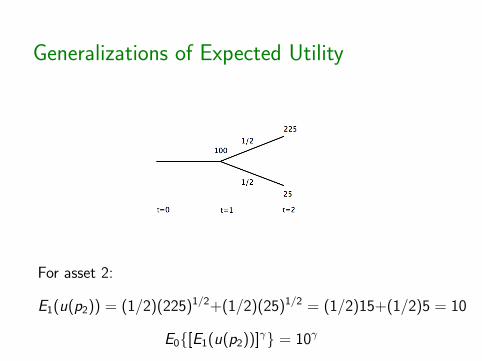
For asset 2:
E1(u(p2)) = (1/2)(225)1/2+(1/2)(25)1/2 = (1/2)15+(1/2)5 = 10
E0{[E1(u(p2))]γ} = 10γ

Generalizations of Expected Utility
For asset 2:E0{[E1(u(p2))]γ} = 10γ
E0[u(p1)] = 100.
Generalizations of Expected Utility
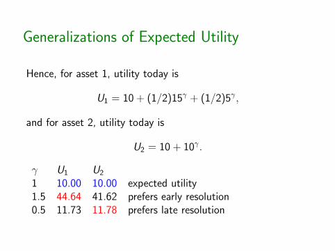
Hence, for asset 1, utility today is
U1 = 10 + (1/2)15γ + (1/2)5γ,
and for asset 2, utility today is
U2 = 10 + 10γ.
γ U1 U2
1 10.00 10.00 expected utility1.5 44.64 41.62 prefers early resolution0.5 11.73 11.78 prefers late resolution
Generalizations of Expected Utility
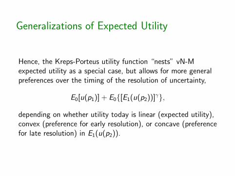
Hence, the Kreps-Porteus utility function “nests” vN-Mexpected utility as a special case, but allows for more generalpreferences over the timing of the resolution of uncertainty,
E0[u(p1)] + E0{[E1(u(p2))]γ},
depending on whether utility today is linear (expected utility),convex (preference for early resolution), or concave (preferencefor late resolution) in E1(u(p2)).
Generalizations of Expected Utility
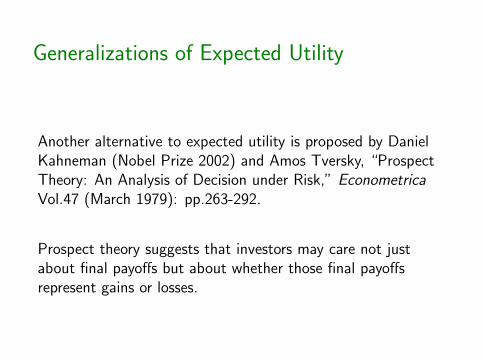
Another alternative to expected utility is proposed by DanielKahneman (Nobel Prize 2002) and Amos Tversky, “ProspectTheory: An Analysis of Decision under Risk,” EconometricaVol.47 (March 1979): pp.263-292.
Prospect theory suggests that investors may care not justabout final payoffs but about whether those final payoffsrepresent gains or losses.
Generalizations of Expected Utility
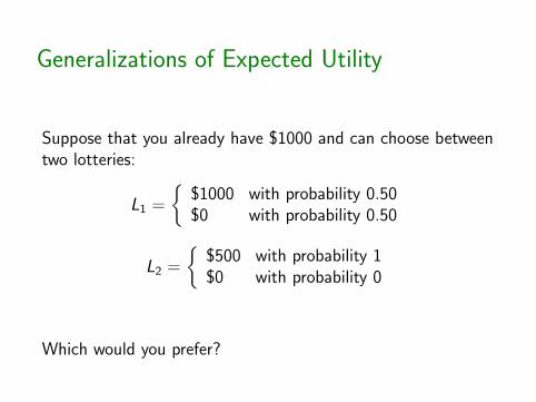
Suppose that you already have $1000 and can choose betweentwo lotteries:
L1 =
{$1000 with probability 0.50$0 with probability 0.50
L2 =
{$500 with probability 1$0 with probability 0
Which would you prefer?
Generalizations of Expected Utility
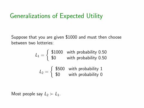
Suppose that you are given $1000 and must then choosebetween two lotteries:
L1 =
{$1000 with probability 0.50$0 with probability 0.50
L2 =
{$500 with probability 1$0 with probability 0
Most people say L2 � L1.

Generalizations of Expected Utility
Suppose instead that you are given $2000 and must thenchoose between two lotteries:
L3 =
{−$1000 with probability 0.50$0 with probability 0.50
L4 =
{−$500 with probability 1$0 with probability 0
Which would you prefer?
Generalizations of Expected Utility
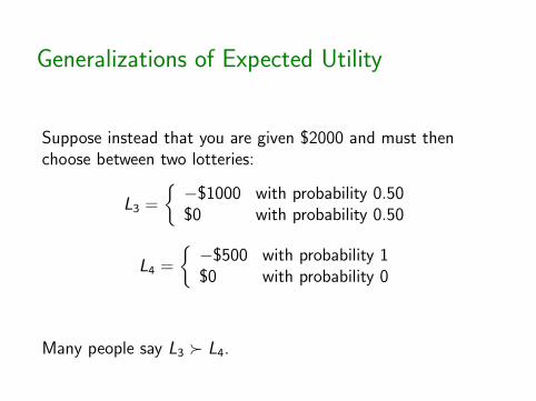
Suppose instead that you are given $2000 and must thenchoose between two lotteries:
L3 =
{−$1000 with probability 0.50$0 with probability 0.50
L4 =
{−$500 with probability 1$0 with probability 0
Many people say L3 � L4.

Generalizations of Expected Utility
But in terms of final payoffs, L1 is identical to L3 and L2 isidentical to L4:
L1 =
{$1000 + $1000 with probability 0.50$1000 + $0 with probability 0.50
L2 =
{$1000 + $500 with probability 1$1000 + $0 with probability 0
L3 =
{$2000− $1000 with probability 0.50$2000 + $0 with probability 0.50
L4 =
{$2000− $500 with probability 1$2000 + $0 with probability 0
suggesting that respondents do care about gains versus losses.

Generalizations of Expected Utility
Expected utility remains the dominant framework for analyzingeconomic decision-making under uncertainty.
But a very active line of ongoing research continues to explorealternatives and generalizations.


![Economics (ECON) ECON 1402 [0.5 credit] Also listed as ...](https://static.fdocuments.in/doc/165x107/6157d782ce5a9d02d46fb3da/economics-econ-econ-1402-05-credit-also-listed-as-.jpg)