Microeconomics Business Operations. Warm Up What is microeconomics?

1
ECON 312/302: MICROECONOMICS II
Lecture 6: W/C 7th March 2016
FACTOR MARKETS 1
Dr Ebo Turkson
Chapter 15
Factor Markets
Part 1

2
15 - 3 Copyright © 2012 Pearson Education. All rights reserved.
Topics
• Competitive Factor Market.
Competitive factor and output markets
• Effect of Monopolies on Factor Markets.
Competitive factor and monopolized output
markets
Monopolized factor and Competitive output
markets
Monopolist in successive markets
15 - 4 Copyright © 2012 Pearson Education. All rights reserved.
Topics
• Monopsony.
the only buyer of a good in a given market.
• Welfare Effects
A comparative Analysis
3
15 - 5 Copyright © 2012 Pearson Education. All rights reserved.
Competitive Factor Market
• Factor markets are competitive when
there are many small buyers and sellers.
• Here the firm is a price taker. i.e. the
wage rate is given (w is given).
15 - 6 Copyright © 2012 Pearson Education. All rights reserved.
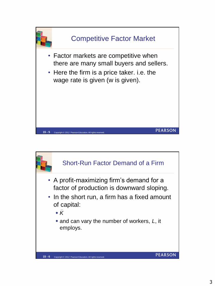
Short-Run Factor Demand of a Firm
• A profit-maximizing firm’s demand for a
factor of production is downward sloping.
• In the short run, a firm has a fixed amount
of capital:
K
and can vary the number of workers, L, it
employs.
4
15 - 7 Copyright © 2012 Pearson Education. All rights reserved.
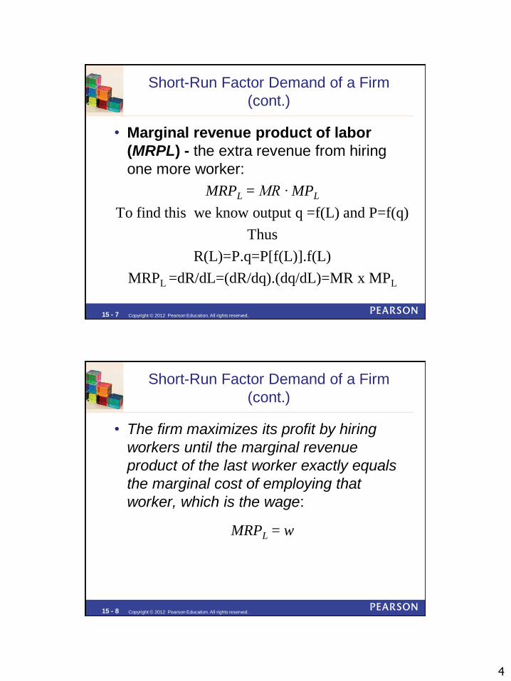
Short-Run Factor Demand of a Firm
(cont.)
• Marginal revenue product of labor
(MRPL) - the extra revenue from hiring
one more worker:
MRPL = MR ∙ MPL
To find this we know output q =f(L) and P=f(q)
Thus
R(L)=P.q=P[f(L)].f(L)
MRPL =dR/dL=(dR/dq).(dq/dL)=MR x MPL
15 - 8 Copyright © 2012 Pearson Education. All rights reserved.
Short-Run Factor Demand of a Firm
(cont.)
• The firm maximizes its profit by hiring
workers until the marginal revenue
product of the last worker exactly equals
the marginal cost of employing that
worker, which is the wage:
MRPL = w

5
15 - 9 Copyright © 2012 Pearson Education. All rights reserved.
Short-Run Factor Demand of a Firm
(cont.)
• A competitive firm faces an infinitely
elastic demand for its output at the market
price, p, so:
MR = p
and
MRPL = p ∙ MPL
15 - 10 Copyright © 2012 Pearson Education. All rights reserved.
Short-Run Factor Demand of a Firm
(cont.)
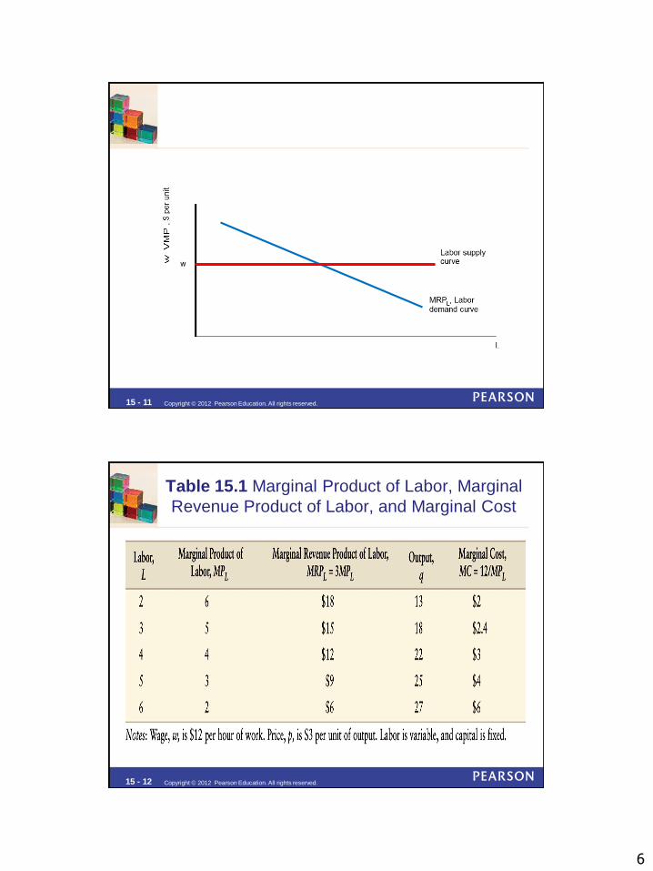
• The competitive firm hires labor to the point at
which:
MRPL = p ∙ MPL = w (1)
• The wage line is the supply of labor the firm faces.
It is horizontal (infinitely elastic)
• The marginal revenue product of labor curve,
MRPL, is the firm’s demand curve for labor
Its downward sloping because although P is fixed MPL
declines as more labour is employed.
6
15 - 11 Copyright © 2012 Pearson Education. All rights reserved.
15 - 12 Copyright © 2012 Pearson Education. All rights reserved.
Table 15.1 Marginal Product of Labor, Marginal
Revenue Product of Labor, and Marginal Cost

7
15 - 13 Copyright © 2012 Pearson Education. All rights reserved.
Figure 15.1 The Relationship Between
Labor Market and Output Market Equilibriaw
,V
MP
L, $ p
er
unit
Labor supplycurve
MRPL, Labor
demand curve
L, Workers per hour
620 3 4 5
(a) Labor Profit-Maximizing Condition
6
w = 12
9
18
15
MC
,p, $ p
er
unit
MC
p
27130 18 22 25
2
3
2.4
6
4
q, Units of output per hour
(b) Output Profit-Maximizing Condition
15 - 14 Copyright © 2012 Pearson Education. All rights reserved.
Profit Maximization Using Labor or Output
• The output profit-maximizing condition from
Chapter 8, MC = p, is equivalent to the labor
profit-maximizing condition in Equation 15.1.
• By dividing Equation 1 by MPL , we find that:
MCMP
wp
L
8
15 - 15 Copyright © 2012 Pearson Education. All rights reserved.
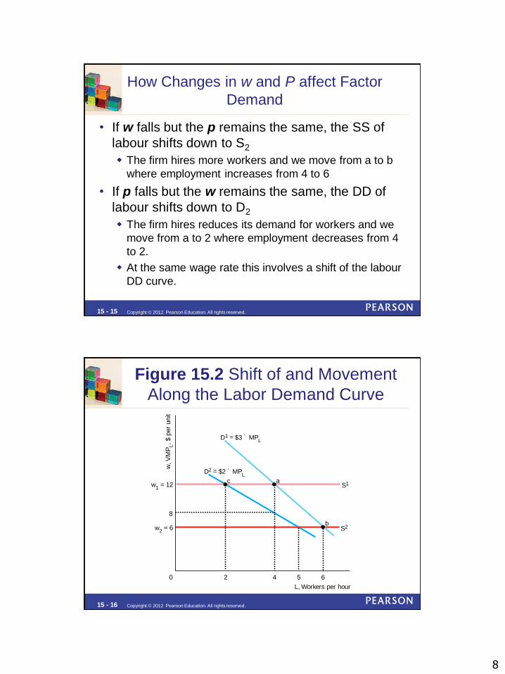
How Changes in w and P affect Factor
Demand
• If w falls but the p remains the same, the SS of
labour shifts down to S2
The firm hires more workers and we move from a to b
where employment increases from 4 to 6
• If p falls but the w remains the same, the DD of
labour shifts down to D2
The firm hires reduces its demand for workers and we
move from a to 2 where employment decreases from 4
to 2.
At the same wage rate this involves a shift of the labour
DD curve.
15 - 16 Copyright © 2012 Pearson Education. All rights reserved.
Figure 15.2 Shift of and Movement
Along the Labor Demand Curve
w,V
MP
L, $ p
er
unit
542 6
D2 = $2 ´ MPL
D1 = $3 ´ MPL
L, Workers per hour
0
8
w1
= 12
w2
= 6
S1
S2
a
b
c
9
15 - 17 Copyright © 2012 Pearson Education. All rights reserved.
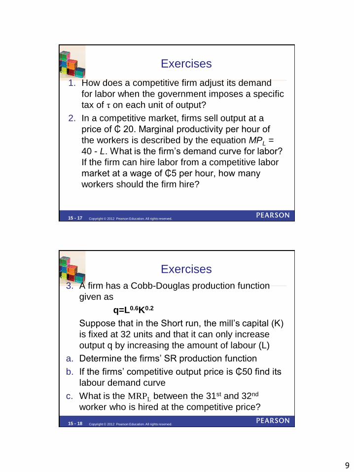
Exercises
1. How does a competitive firm adjust its demand
for labor when the government imposes a specific
tax of τ on each unit of output?
2. In a competitive market, firms sell output at a
price of ₵ 20. Marginal productivity per hour of
the workers is described by the equation MPL =
40 - L. What is the firm’s demand curve for labor?
If the firm can hire labor from a competitive labor
market at a wage of ₵5 per hour, how many
workers should the firm hire?
15 - 18 Copyright © 2012 Pearson Education. All rights reserved.
Exercises
3. A firm has a Cobb-Douglas production function
given as
q=L0.6K0.2
Suppose that in the Short run, the mill’s capital (K)
is fixed at 32 units and that it can only increase
output q by increasing the amount of labour (L)
a. Determine the firms’ SR production function
b. If the firms’ competitive output price is ₵50 find its
labour demand curve
c. What is the MRPL between the 31st and 32nd
worker who is hired at the competitive price?
10
15 - 19 Copyright © 2012 Pearson Education. All rights reserved.
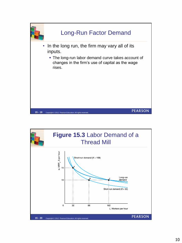
Long-Run Factor Demand
• In the long run, the firm may vary all of its
inputs.
The long-run labor demand curve takes account of
changes in the firm’s use of capital as the wage
rises.
15 - 20 Copyright © 2012 Pearson Education. All rights reserved.
Figure 15.3 Labor Demand of a
Thread Mill
11
15 - 21 Copyright © 2012 Pearson Education. All rights reserved.
Exercises
4. A firm has a Cobb-Douglas production function
given as
q=ALαKβ
a. Solve for the factor demand functions
b. If the firms’ competitive output price is p find the
wage rate
c. What is the share of the firms revenue paid to
labour and capital?
d. If α=0.6, β=0.2 and A=1 find the LR labour and
capital demand curve equations
15 - 22 Copyright © 2012 Pearson Education. All rights reserved.
Short-Run Factor Demand of a Firm
(cont.)
• The firm maximizes its profit by hiring
workers until the marginal revenue
product of the last worker exactly equals
the marginal cost of employing that
worker, which is the wage:
MRPL = w
12
15 - 23 Copyright © 2012 Pearson Education. All rights reserved.
Short-Run Factor Demand of a Firm
(cont.)
• The competitive firm hires labor to the point at
which:
MRPL = p ∙ MPL = w (1)
• The wage line is the supply of labor the firm faces.
It is horizontal (infinitely elastic)
• The marginal revenue product of labor curve,
MRPL, is the firm’s demand curve for labor
Its downward sloping because although P is fixed MPL
declines as more labour is employed.
15 - 24 Copyright © 2012 Pearson Education. All rights reserved.
Exercises
3. A firm has a Cobb-Douglas production function
given as
q=L0.6K0.2
Suppose that in the Short run, the mill’s capital (K)
is fixed at 32 units and that it can only increase
output q by increasing the amount of labour (L)
a. Determine the firms’ SR production function
b. If the firms’ competitive output price is ₵50 find its
labour demand curve
c. What is the MRPL between the 31st and 32nd
worker who is hired at the competitive price?

13
15 - 25 Copyright © 2012 Pearson Education. All rights reserved.
Long-Run Factor Demand
• In the long run, the firm may vary all of its
inputs.
The long-run labor demand curve takes account of
changes in the firm’s use of capital as the wage
rises.
15 - 26 Copyright © 2012 Pearson Education. All rights reserved.
Figure 15.3 Labor Demand of a
Thread Mill

14
15 - 27 Copyright © 2012 Pearson Education. All rights reserved.
Exercises
4. A firm has a Cobb-Douglas production function
given as
q=ALαKβ
a. Solve for the factor demand functions
b. If the firms’ competitive output price is p find the
wage rate
c. What is the share of the firms revenue paid to
labour and capital?
d. If α=0.6, β=0.2 and A=1 find the LR labour and
capital demand curve equations