
Ecology of Flows and Drift Wave Turbulence: Reduced Models ...
148
UNIVERSITY OF CALIFORNIA, SAN DIEGO Ecology of Flows and Drift Wave Turbulence: Reduced Models and Applications A dissertation submitted in partial satisfaction of the requirements for the degree Doctor of Philosophy in Engineering Sciences (Engineering Physics) by Rima Hajjar Committee in charge: Professor George R. Tynan, Chair Professor Patrick H. Diamond, Co-Chair Professor Farhat Beg Professor Kevin Quest Professor Daniel Tartakovsky 2018
Transcript of Ecology of Flows and Drift Wave Turbulence: Reduced Models ...
UNIVERSITY OF CALIFORNIA, SAN DIEGO
Ecology of Flows and Drift Wave Turbulence: Reduced Models and Applications
A dissertation submitted in partial satisfaction of therequirements for the degree
Doctor of Philosophy
in
Engineering Sciences (Engineering Physics)
by
Rima Hajjar
Committee in charge:
Professor George R. Tynan, ChairProfessor Patrick H. Diamond, Co-ChairProfessor Farhat BegProfessor Kevin QuestProfessor Daniel Tartakovsky
2018
Copyright
Rima Hajjar, 2018
All rights reserved.
The dissertation of Rima Hajjar is approved, and it is accept-
able in quality and form for publication on microfilm and
electronically:
Co-Chair
Chair
University of California, San Diego
2018
iii
DEDICATION
To my father Joseph, my mother Bernadette,
to my sisters Nisrine, Rosine, Nelly, Soha and Nicole,
and most importantly, to my husband Avram.
iv
EPIGRAPH
Alice: Would you tell me, please, which way I ought to go from here?
The Cheshire Cat: That depends a good deal on where you want to get to.
Alice: I don’t much care where.
The Cheshire Cat: Then it doesn’t much matter which way you go.
Alice: ...So long as I get somewhere.
The Cheshire Cat: Oh, you’re sure to do that, if only you walk long enough.
—Lewis Caroll, Alice in wonderland
v
TABLE OF CONTENTS
Signature Page . . . . . . . . . . . . . . . . . . . . . . . . . . . . . . . . . . . . . . . iii
Dedication . . . . . . . . . . . . . . . . . . . . . . . . . . . . . . . . . . . . . . . . . . iv
Epigraph . . . . . . . . . . . . . . . . . . . . . . . . . . . . . . . . . . . . . . . . . . . v
Table of Contents . . . . . . . . . . . . . . . . . . . . . . . . . . . . . . . . . . . . . . vi
List of Figures . . . . . . . . . . . . . . . . . . . . . . . . . . . . . . . . . . . . . . . . ix
List of Tables . . . . . . . . . . . . . . . . . . . . . . . . . . . . . . . . . . . . . . . . xi
Acknowledgements . . . . . . . . . . . . . . . . . . . . . . . . . . . . . . . . . . . . . xii
Vita . . . . . . . . . . . . . . . . . . . . . . . . . . . . . . . . . . . . . . . . . . . . . xiv
Abstract of the Dissertation . . . . . . . . . . . . . . . . . . . . . . . . . . . . . . . . . xv
Chapter 1 INTRODUCTION . . . . . . . . . . . . . . . . . . . . . . . . . . . . . 11.1 Nuclear Fusion: Concepts and Definitions . . . . . . . . . . . . . . 11.2 Classical, Neoclassical, and Anomalous Transport . . . . . . . . . . 41.3 Turbulence and Instabilities . . . . . . . . . . . . . . . . . . . . . . 61.4 Drift Waves and Drift Wave Instabilities . . . . . . . . . . . . . . . 7
1.4.1 Linear Analysis and Linear Solutions . . . . . . . . . . . . 71.4.2 Hasegawa-Mima Equation . . . . . . . . . . . . . . . . . . 131.4.3 Hasegawa-Wakatani Equations . . . . . . . . . . . . . . . . 14
1.5 The Drift Wave- Zonal Flow Relation . . . . . . . . . . . . . . . . 151.6 The Drift Wave-Axial Flow Relation . . . . . . . . . . . . . . . . . 191.7 Dissertation Outline . . . . . . . . . . . . . . . . . . . . . . . . . . 21
Chapter 2 THE ECOLOGY OF FLOWS AND DRIFT WAVE TURBULENCE INCSDX: A MODEL . . . . . . . . . . . . . . . . . . . . . . . . . . . . . 262.1 INTRODUCTION . . . . . . . . . . . . . . . . . . . . . . . . . . 262.2 THE MODEL AND ITS STRUCTURE . . . . . . . . . . . . . . . 312.3 CALCULATING THE TURBULENT FLUXES . . . . . . . . . . . 37
2.3.1 The Turbulent Particle Flux . . . . . . . . . . . . . . . . . 372.3.2 The Vorticity Flux, the Perpendicular Reynolds Stress and
theReynolds Work . . . . . . . . . . . . . . . . . . . . . . . . 40
2.4 THE PARALLEL REYNOLDS STRESS 〈vxvz〉 . . . . . . . . . . . 422.4.1 Calculating the Expression for 〈vxvz〉 . . . . . . . . . . . . 44
vi
2.4.2 Analogy to Pipe Flow: A Simple Approach to the Physics ofthe 〈kmkz〉 Correlator . . . . . . . . . . . . . . . . . . . . . 45
2.5 THE RADIAL MIXING LENGTH lmix . . . . . . . . . . . . . . . 482.5.1 Case of a purely azimuthal shear . . . . . . . . . . . . . . . 482.5.2 Case of azimuthal and axial shear . . . . . . . . . . . . . . 50
2.6 SUMMARY AND DISCUSSION OF THE MODEL . . . . . . . . 512.7 REDUCING THE MODEL . . . . . . . . . . . . . . . . . . . . . . 52
2.7.1 Equations and Fluxes . . . . . . . . . . . . . . . . . . . . . 532.7.2 Closure by Slaving . . . . . . . . . . . . . . . . . . . . . . 54
2.8 CONCLUSION . . . . . . . . . . . . . . . . . . . . . . . . . . . . 542.9 Acknowledgments . . . . . . . . . . . . . . . . . . . . . . . . . . 59
Chapter 3 MODELING ENHANCED CONFINEMENT IN DRIFT WAVE TURBU-LENCE . . . . . . . . . . . . . . . . . . . . . . . . . . . . . . . . . . . 603.1 Introduction . . . . . . . . . . . . . . . . . . . . . . . . . . . . . . 603.2 Structure of the 3-Field Reduced Model. . . . . . . . . . . . . . . . 64
3.2.1 The Mixing Length . . . . . . . . . . . . . . . . . . . . . . 663.2.2 Expressions for the Turbulent Fluxes . . . . . . . . . . . . . 673.2.3 Viscosity and Diffusion Coefficients . . . . . . . . . . . . . 70
3.3 Model Predictions of Plasma Profiles. . . . . . . . . . . . . . . . . 713.3.1 Diffusive Vorticity Flux: Π =−χ∂xu . . . . . . . . . . . . 723.3.2 Vorticity Flux with Residual Stress: Π = Πres−χ∂xu . . . . 78
3.4 Validation Metrics for Model Comparison with Experiment. . . . . 803.5 What is the Criterion for Turbulence Suppression? . . . . . . . . . . 823.6 Discussion ans Conclusions. . . . . . . . . . . . . . . . . . . . . . 843.7 Acknowledgments . . . . . . . . . . . . . . . . . . . . . . . . . . 85
Chapter 4 DYNAMICS OF ZONAL SHEAR COLLAPSE FOR HYDRODYNAMICELECTRONS . . . . . . . . . . . . . . . . . . . . . . . . . . . . . . . . 904.1 Introduction . . . . . . . . . . . . . . . . . . . . . . . . . . . . . . 904.2 Basic System and Linear Stability Analysis . . . . . . . . . . . . . 944.3 Reduced Model . . . . . . . . . . . . . . . . . . . . . . . . . . . . 97
4.3.1 The equations . . . . . . . . . . . . . . . . . . . . . . . . . 974.4 Expressions for the Turbulent Fluxes . . . . . . . . . . . . . . . . . 99
4.4.1 The Particle Flux: 〈nvx〉 . . . . . . . . . . . . . . . . . . . 1004.4.2 The Vorticity Flux: 〈vx∇2
⊥φ〉 . . . . . . . . . . . . . . . . . 1014.4.3 Fluxes and Reynolds Work in Adiabatic and Hydrodynamic
Limits. . . . . . . . . . . . . . . . . . . . . . . . . . . . . 1034.5 Simplification by Slaving: A Predator-Prey Model . . . . . . . . . . 1054.6 Fate of Zonal Flows in the Hydrodynamic Limit α 1 . . . . . . . 107
4.6.1 Physical Picture: Energy-Momentum Flux Physics . . . . . 1084.6.2 Scalings of Transport Fluxes with α . . . . . . . . . . . . . 1094.6.3 Potential Vorticity Mixing and Zonal Shear Collapse . . . . 111
vii
4.7 Relevance to Density Limit nG . . . . . . . . . . . . . . . . . . . . 1134.8 Conclusion . . . . . . . . . . . . . . . . . . . . . . . . . . . . . . 1154.9 Acknowledgments . . . . . . . . . . . . . . . . . . . . . . . . . . 118
Chapter 5 SUMMARY AND FUTURE DIRECTIONS . . . . . . . . . . . . . . . . 120
Bibliography . . . . . . . . . . . . . . . . . . . . . . . . . . . . . . . . . . . . . . . . 124
viii
LIST OF FIGURES
Figure 1.1: Fusion reaction rates versus temperature. . . . . . . . . . . . . . . . . . . 3Figure 1.2: Magnetic configuration inside a tokamak. . . . . . . . . . . . . . . . . . . 4Figure 1.3: Controlled Sheared Decorrelation eXperiment (CSDX) . . . . . . . . . . . 5Figure 1.4: Geometry of the problem, showing the density gradient and the magnetic
field vector. . . . . . . . . . . . . . . . . . . . . . . . . . . . . . . . . . . 7Figure 1.5: Drift wave perturbation reproduced from [Pec13]. The solid line indicates
a contour of constant density, while the electric fields and the ion velocitiesare indicated by small arrows. Charge densities are indicated by + and -symbols. Regions with enhanced density are shaded for clarity. . . . . . . 10
Figure 1.6: Direct energy cascade in 3D turbulent systems. . . . . . . . . . . . . . . . 16Figure 1.7: Dual cascade in 2D turbulent systems. . . . . . . . . . . . . . . . . . . . . 16Figure 1.8: Tilting and shearing of the eddies. . . . . . . . . . . . . . . . . . . . . . . 17Figure 1.9: Generation of zonal flows by triad coupling. The wavenumbers of the drift
waves are bigger than that of the zonal flow:~k1,~k2~kZF . . . . . . . . . . 18Figure 1.10: Spectral imbalance in the parallel wavenumber space [LDXT16]. . . . . . 20Figure 1.11: Scaling comparison between standard tokamak, tokamak transport barrier
regime, and CSDX [CAT+16]. . . . . . . . . . . . . . . . . . . . . . . . . 21Figure 1.12: (De)-evolutionary tree of plasma models showing the organization of the
dissertation. . . . . . . . . . . . . . . . . . . . . . . . . . . . . . . . . . . 25
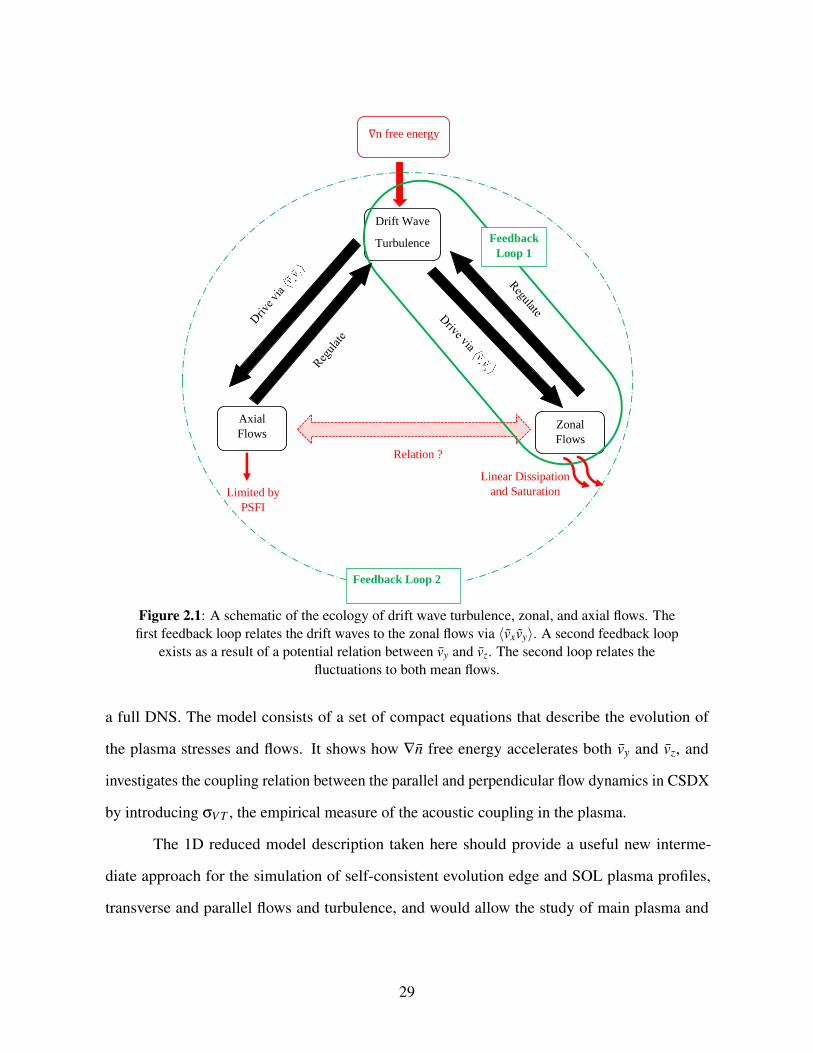
Figure 2.1: A schematic of the ecology of drift wave turbulence, zonal, and axial flows.The first feedback loop relates the drift waves to the zonal flows via 〈vxvy〉.A second feedback loop exists as a result of a potential relation between vyand vz. The second loop relates the fluctuations to both mean flows. . . . . 29
Figure 2.2: Feedback loop between axial and zonal flows via 〈kmkz〉. A strong zonalflow shear can affect the axial flow. . . . . . . . . . . . . . . . . . . . . . 43
Figure 2.3: The future of CSDX: particle and axial momentum sources enhance theinteractions between flows and turbulence, and generate further couplingbetween the axial and perpendicular flow dynamics. . . . . . . . . . . . . 58
Figure 3.1: Experimental plasma profiles at different magnetic field values. Reprintedwith permission from Cui et al., Physics of Plasmas, 22, 050704 (2015).Copyright 2015 AIP Publishing. [CTD+15] . . . . . . . . . . . . . . . . . 62
Figure 3.2: Density profiles for S = 10 and S = 104 for increasing B. . . . . . . . . . . 74Figure 3.3: Fluxes for S = 104 for increasing B. . . . . . . . . . . . . . . . . . . . . . 75Figure 3.4: Diffusion coefficient for increasing B. . . . . . . . . . . . . . . . . . . . . 76Figure 3.5: Particle flux at S = 10 for increasing B and particle flux at constant B and
increasing S : Sblue < Sred < Sgreen < Sblack. . . . . . . . . . . . . . . . . . 76Figure 3.6: Purely outward particle flux at sufficiently long time . . . . . . . . . . . . 77Figure 3.7: Velocity shear, Reynolds Force and Reynolds work for increasing B at S = 104. 77Figure 3.8: Profiles with Πres and Dirichlet boundary conditions for cu = 6 and cu = 600. 86
ix
Figure 3.9: Profiles with Πres and Neumann boundary conditions for increasing B. . . . 87Figure 3.10: Profiles for l0 = 10−3ρs and increasing B. . . . . . . . . . . . . . . . . . . 88Figure 3.11: Profiles for Pr = 65000 and increasing B. Solid and dashed plots correspond
to data at t1 and t2 respectively. . . . . . . . . . . . . . . . . . . . . . . . 88Figure 3.12: PRe−tot as function of 1/Ln for increasing B. . . . . . . . . . . . . . . . . . 89Figure 3.13: RT time variations at x = 0.1, 0.6 and 0.8 (Blue, Green, Brown) for S = 40. 89Figure 3.14: RDT variations for S = 10 and increasing B . . . . . . . . . . . . . . . . . . 89
Figure 4.1: Outgoing wave energy flux and incoming momentum flux from/to perturbation.109Figure 4.2: A jump in the flow shear (in blue) over a scale length D is equivalent to a
vorticity gradient on that scale. . . . . . . . . . . . . . . . . . . . . . . . . 111Figure 4.3: Analogy of PV conservation in geostrophic waves and drift waves: (a)
change in local vorticity ~ω of a fluid element between θ1 and θ2 forces aflow generation, (b) density variation along the ∇n line from position 1 toposition 2 triggers a change in the flow (i.e., vorticity) so to conserve q. . . 112
Figure 4.4: Profile evolution in the hydrodynamic limit. The diagram shows a feedbackloop between the density and temperature via variations of α. A potentialpath for the development of MHD modes is also indicated. Inward turbulencespreading and steepening of adjacent ∇T from a state 1© (in blue) to a state2© (in red) are shown on the left. . . . . . . . . . . . . . . . . . . . . . . . 119
x
LIST OF TABLES
Table 1.1: Characteristics of CSDX plasma. . . . . . . . . . . . . . . . . . . . . . . . 22
Table 3.1: Scaling of kr with B . . . . . . . . . . . . . . . . . . . . . . . . . . . . . . 72Table 3.2: Particle loss rate 1/τ for increasing B. . . . . . . . . . . . . . . . . . . . . 82
Table 4.1: Scalings of the turbulent enstrophy ε, transport fluxes and vorticity gradientwith α in both adiabatic and hydrodynamic regimes. . . . . . . . . . . . . . 110
xi
ACKNOWLEDGEMENTS
Firstly, I would like to express my sincere gratitude to Prof. Patrick H. Diamond and Prof.
George R. Tynan for their continuous support of my PhD study, for their patience, motivation and
immense knowledge. Their guidance helped me complete a successful PhD degree and present
a decent scientific research. I would like to thank them for welcoming me into their research
group. My deepest appreciation goes to my lead academic advisor Patrick Diamond. Not only
was he the perfect PhD advisor, but also the best academic mentor I could have ever imagined.
His deep knowledge and sharp and constructive critic helped me become a better scientist. I will
be forever grateful for his patience and his help.
I would like to thank the members of my dissertation committee: Prof. Farhat Beg, Prof.
Kevin Quest, and Prof. Daniel Tartakovsky. Special gratitude goes to Prof. Tartakovsky. I will
always remember the fluid course he taught me as part of the PhD course requirements.
My sincere thanks also go to people of the lunch club: Leo Chousal, Rollie Hernandez,
Dr. Rongjie Hong, Dr. Saikat Thakur, Dr. Jonathan Yu, Dr. Anze Zloznik, and soon to be Dr.
Shota Abe, Dr. Jiacong Li and Dr. Michael J. Simmonds. I would like to thank each and every
one of them for the stimulating discussions we had, regarding both physics and non-physics
topics.
I would also like to thank Zachary Dake, Patrick Mallon and Lydia Ramirez from the
Mechanical and Aerospace Engineering department, as well as the assistant Dean and Director of
the Students Affairs and Admissions April Bjornsen for providing an immense help overcoming
many of the technical problems during my PhD. I am deeply appreciative of their assistance.
Of course, my deepest gratitude goes to my family: my father Joseph, my mother
Berandette, and my sisters: Nisrine, Rosine, Nelly, Soha and Nicole. Despite not being physically
present around me, I am sure they kept me in their hearts and minds. My family played a major
and important role in supporting all the decisions I took, decisions that allowed me to reach the
point of defending my PhD. I would also like to thank my mother-in-law for her assistance and
xii
support.
Lastly and most importantly, I am forever grateful to my husband Avram Dalton. Avram
was my source of motivation during the lonely times I spent wondering when I will finish my
PhD, or if I will ever finish it. I feel he shared with me the hurdles, the efforts, the good and the
bad of this PhD. I thank him for being the ONLY constant sound of reason and sanity during the
seven years I spent at UCSD, and I dedicate this degree to him.
Chapter 2 is a reprint of the material as it appears in the publication ”The Ecology of
Flows and Drift Wave Turbulence in CSDX: a Model” in the Journal of Physics of Plasmas 25,
022301 (2018). Hajjar R. J., Diamond P.H., Tynan G.R., American Institute of Physics, 2018.
The dissertation author was the primary investigator and author of this article.
Chapter 3 is a reprint of the material as it appears in the publication ”Modeling Enhanced
Confinement in Drift-Wave Turbulence” in the Journal of Physics of Plasmas 24, 062106 (2017).
Hajjar R. J., Diamond P. H., Ashourvan A., Tynan G. R, American Institute of Physics, 2017.
The dissertation author was the primary investigator and author of this article.
Chapter 4 is currently being prepared for submission for publication in ”On the Dynamics
of Zonal Shear Layer Collapse at High Density” in the Journal of Physics of Plasmas 2018.
Hajjar R. J., Diamond P. H., Malkov M., American Institute of Physics, 2018. The dissertation
author was the primary investigator and author of this article.
xiii
VITA
2007 B. S. in Physics, Lebanese University, Beirut, Lebanon.
2010 M. S. in Physics, American University of Beirut, Beirut, Lebanon.
2011-2018 Graduate Research Assistant and Teaching Assistant, University of California,San Diego, USA.
2018 Ph. D. in Engineering Sciences (Engineering Physics), University of California,San Diego, USA.
PUBLICATIONS
R. J. Hajjar, P. H. Diamond, M. Malkov, “On the Dynamics of Zonal Shear Layer Collapse atHigh Density”, Journal of Physics of Plasmas, (under preparation for submission for publication)
R. J. Hajjar, P. H. Diamond, G. R. Tynan, “The Ecology of Flows and Drift Wave Turbulence inCSDX: a Model”, Journal of Physics of Plasmas, 25, 022301, 2018.
R. J. Hajjar, P. H. Diamond, A. Ashourvan, G. R. Tynan,“Modeling Enhanced Confinement inDrift Wave Turbulence”, Journal Physics of Plasmas, 24, 062106, 2017.
R. Hajjar, E. M. Hollmann, S. I. Krashenninikov, R. P. Doerner, “Modeling of Aluminum ImpurityEntrainment in the PISCES-A He+ Plasma”, Journal of Nuclear Materials, 463, 664-667, 2015.
R. Hong, J. C. Li, S. Chakraborty Thakur, R. J. Hajjar, P. H. Diamond, G. R. Tynan, “Tracingthe Pathway from Drift-Wave Turbulence with Broken Symmetry to the Production of ShearedAxial Mean Flow”, Physical Review Letters (Accepted for publication)
R. Hong, J. C. Li, R. J. Hajjar, S. Chakraborty Thakur, P. H. Diamond, G. R. Tynan, “Gener-ation of Parasitic Axial Flow by Drift Wave Turbulence with Broken Symmetry: Theory andExperiment”, Journal of Physics of Plasmas (Submitted for publication)
xiv
ABSTRACT OF THE DISSERTATION
Ecology of Flows and Drift Wave Turbulence: Reduced Models and Applications
by
Rima Hajjar
Doctor of Philosophy in Engineering Sciences (Engineering Physics)
University of California, San Diego, 2018
Professor George R. Tynan, ChairProfessor Patrick H. Diamond, Co-Chair
In this dissertation, we present advances in turbulence modeling for magnetically confined
plasmas. We investigate the ecology of microscopic drift wave turbulence and the self-generated
macroscopic flows in magnetically confined plasmas. We formulate reduced models that self-
consistently describe the evolution of turbulence and mean plasma profiles (including flows) and
recover trends obtained from the CSDX device and HL-2A tokamak. The dissertation is divided
to three parts. The first part presents a reduced model that describes the interplay between drift
wave turbulence and zonal and axial flows in the adiabatic plasma of CSDX, where the electron
response is Boltzmann. The model explains how free energy released from the density gradient
xv
accelerates both axial and azimuthal flows in CSDX. A description of the interactions between
the disparate scales of the plasma via the parallel and perpendicular Reynolds stresses 〈vxvz〉 and
〈vxvy〉 is presented. Expressions for these stresses are decomposed into a diffusive component
that relaxes the flow profile, and a residual stress responsible for accelerating the corresponding
flow. Moreover, parallel and perpendicular flow dynamics are described using an extended
mixing length approach. This accounts for the degree of symmetry breaking in the parallel
direction and parametrizes the efficiency of ∇n in driving the axial flow. In the second part of the
dissertation, the relationship between drift waves and zonal flows is examined in depth via a more
specific model. Analytical results obtained from this model confirm the published experimental
data showing a suppression of turbulence with the increase in magnitude of the magnetic field
B. A new criterion for access to enhanced confinement is introduced. This criterion captured
by the dimensionless quantity RDT , compares the production rate of turbulent enstrophy due to
relaxation of the mean profiles, to the corresponding destruction rate via coupling to the mean
flow. When RDT > 1, the profiles steepen and enhanced confinement is accessible. In the third
paper, a novel idea for understanding the physics of the density limit problem in low β tokamaks
is presented. The collapse of the zonal shear flow when the electron response transitions from
Boltzmann to hydrodynamic scaling, along with cooling of the edge and the onset of MHD
activity is predicted by the observation that the zonal flow drive will drop as the electron parallel
diffusion time increases with density. This leads to a simple, verified understanding of the density
limit phenomenon in L-modes.
xvi
Chapter 1
INTRODUCTION
1.1 Nuclear Fusion: Concepts and Definitions
The greatest increase in demand for energy is envisaged to come from developing
countries where, with rapid urbanization, large-scale electricity generation will be required. With
environmental requirements for zero or low CO2 emission sources and the need to invest in a
viable energy mix, new energy sources must be developed. Since the 1950s, nuclear fusion has
been investigated as a means for humans to generate sustainable energy. As an alternative to
burning fossil fuels, nuclear fusion has the potential of producing high outputs of clean energy
that can be easily converted to electric power. In contrast to nuclear fission reactions, controlled
fusion reactions safely release high amount of energy while producing fewer radioactive particles.
In spite of currently remaining an experimental technology for power production, nuclear fusion
will be available as a future energy option, and should acquire a significant role in providing a
sustainable, secure and safe solution to tackle the global energy needs.
Plasma, also referred to as the fourth state of matter, is a hot ionized and charged gas that
can be classified into two categories: a natural plasma that occurs in the Sun, the stars and the
interstellar clouds..., and a laboratory or a man-made plasma. The latter is currently being studied
1
as a potential route to fusion energy. The primary fuel used in experimental fusion power plants
is composed of Hydrogen isotopes. The three nuclear reactions involving hydrogen isotopes are:
21H +2
1 H→32 He+1
0 n+3.27MeV (1.1)
21H +2
1 H→31 H +1
1 H +4.03MeV (1.2)
21H +3
1 H→42 He+1
0 n+17.59MeV (1.3)
Of these, the reaction with the highest cross section is a D-T reaction, where a nucleus of
deuterium (21H) fuses with a nucleus of tritium (3
1H) to produce an alpha particle (42He) and
a neutron. Because of the mass difference between the reactants and products, this reaction
produces an energy excess of 17.6 MeV , carried mostly by the light neutron. In advanced
nuclear reactor designs, the resultant neutron escapes the electromagnetic fields, and reacts with a
plasma breeder blanket composed mainly of Lithium (63Li) composites according to the following
reaction:
10n+6
3 Li→42 He+3
1 H +4.8MeV (1.4)
This reaction produces an additional alpha particle and another tritium nucleus, which
is recycled back to fuel the original (D-T) mixture in the reactor core. Conventional energy
conversion methods are then used to produce electric power out of the 4.8MeV exothermic
energy yielded by the Lithium reaction. Macroscopically, 1 kg of the D-T fuel produces 108kWh
of energy in the nuclear fusion process, enough to provide the requirement of a 1GW electric
power station per day [Wes04]. This means that, while a 103 MW coal-fired power plant requires
2.7 million tons of coal per year, a fusion plant will only require 250 kg of D-T fuel per year,
half of it being deuterium, the other half being tritium [ite].
For the Deuterium-Tritium reaction to occur, the D-T mixture needs to be heated to a
sufficiently high temperature to overcome the Coulomb repulsive force. At a sufficiently high
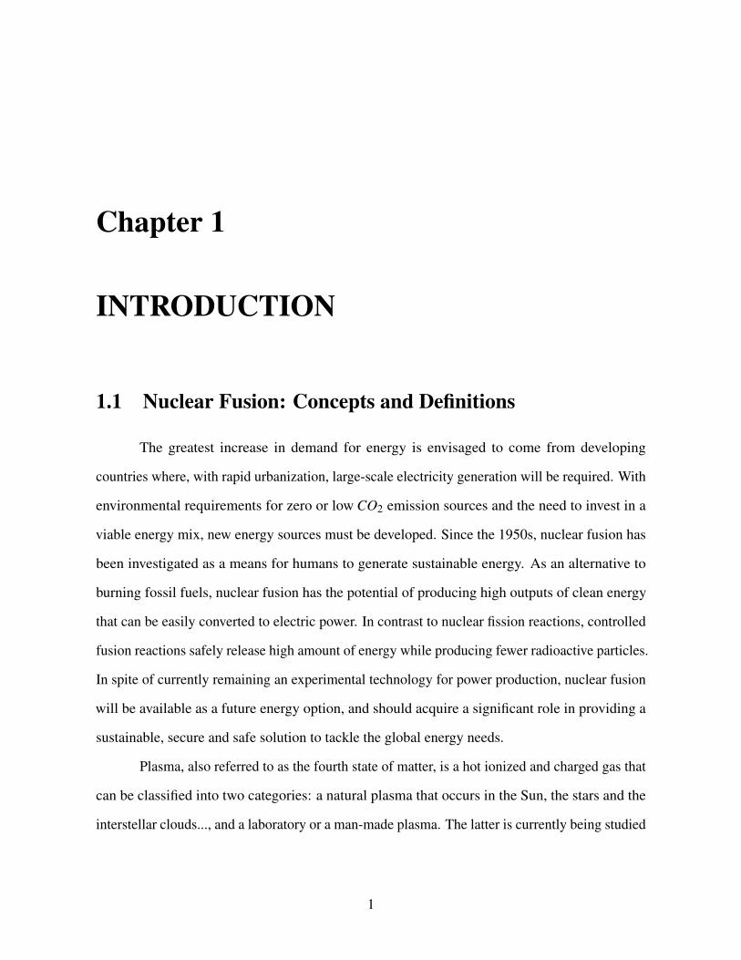
temperature (roughly > 10 keV ), the cross section of the D-T reaction is optimal as shown in
2
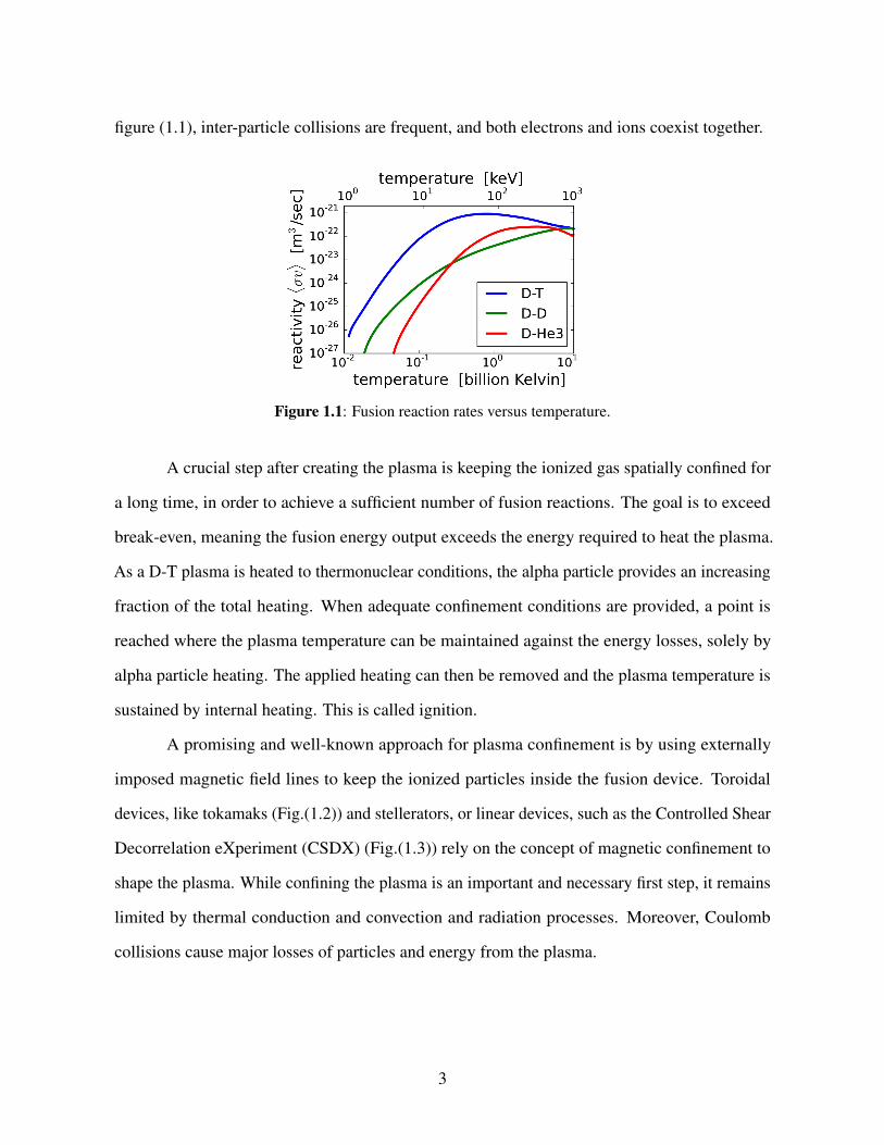
figure (1.1), inter-particle collisions are frequent, and both electrons and ions coexist together.
Figure 1.1: Fusion reaction rates versus temperature.
A crucial step after creating the plasma is keeping the ionized gas spatially confined for
a long time, in order to achieve a sufficient number of fusion reactions. The goal is to exceed
break-even, meaning the fusion energy output exceeds the energy required to heat the plasma.
As a D-T plasma is heated to thermonuclear conditions, the alpha particle provides an increasing
fraction of the total heating. When adequate confinement conditions are provided, a point is
reached where the plasma temperature can be maintained against the energy losses, solely by
alpha particle heating. The applied heating can then be removed and the plasma temperature is
sustained by internal heating. This is called ignition.
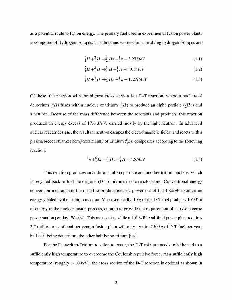
A promising and well-known approach for plasma confinement is by using externally
imposed magnetic field lines to keep the ionized particles inside the fusion device. Toroidal
devices, like tokamaks (Fig.(1.2)) and stellerators, or linear devices, such as the Controlled Shear
Decorrelation eXperiment (CSDX) (Fig.(1.3)) rely on the concept of magnetic confinement to
shape the plasma. While confining the plasma is an important and necessary first step, it remains
limited by thermal conduction and convection and radiation processes. Moreover, Coulomb
collisions cause major losses of particles and energy from the plasma.
3
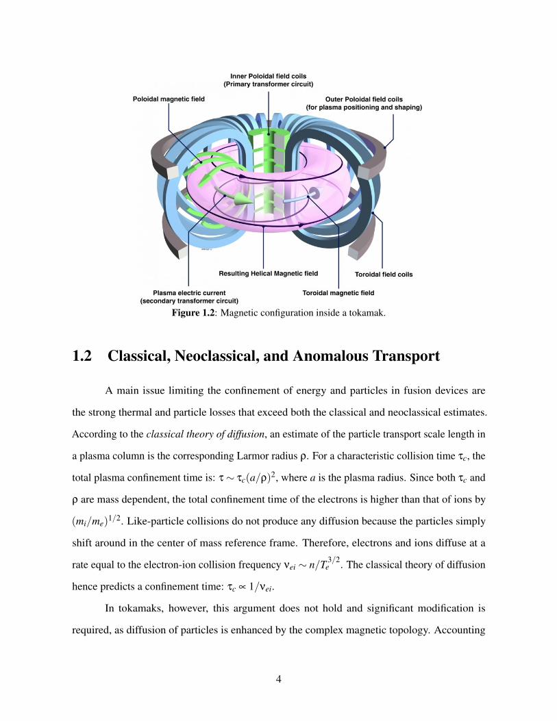
Figure 1.2: Magnetic configuration inside a tokamak.
1.2 Classical, Neoclassical, and Anomalous Transport
A main issue limiting the confinement of energy and particles in fusion devices are
the strong thermal and particle losses that exceed both the classical and neoclassical estimates.
According to the classical theory of diffusion, an estimate of the particle transport scale length in
a plasma column is the corresponding Larmor radius ρ. For a characteristic collision time τc, the
total plasma confinement time is: τ∼ τc(a/ρ)2, where a is the plasma radius. Since both τc and
ρ are mass dependent, the total confinement time of the electrons is higher than that of ions by
(mi/me)1/2. Like-particle collisions do not produce any diffusion because the particles simply
shift around in the center of mass reference frame. Therefore, electrons and ions diffuse at a
rate equal to the electron-ion collision frequency νei ∼ n/T 3/2e . The classical theory of diffusion
hence predicts a confinement time: τc ∝ 1/νei.
In tokamaks, however, this argument does not hold and significant modification is
required, as diffusion of particles is enhanced by the complex magnetic topology. Accounting
4
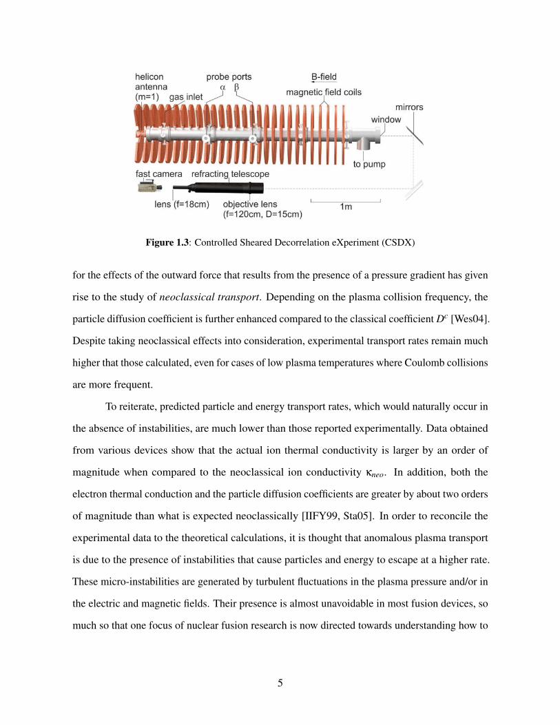
Figure 1.3: Controlled Sheared Decorrelation eXperiment (CSDX)
for the effects of the outward force that results from the presence of a pressure gradient has given
rise to the study of neoclassical transport. Depending on the plasma collision frequency, the
particle diffusion coefficient is further enhanced compared to the classical coefficient Dc [Wes04].
Despite taking neoclassical effects into consideration, experimental transport rates remain much
higher that those calculated, even for cases of low plasma temperatures where Coulomb collisions
are more frequent.
To reiterate, predicted particle and energy transport rates, which would naturally occur in
the absence of instabilities, are much lower than those reported experimentally. Data obtained
from various devices show that the actual ion thermal conductivity is larger by an order of
magnitude when compared to the neoclassical ion conductivity κneo. In addition, both the
electron thermal conduction and the particle diffusion coefficients are greater by about two orders
of magnitude than what is expected neoclassically [IIFY99, Sta05]. In order to reconcile the
experimental data to the theoretical calculations, it is thought that anomalous plasma transport
is due to the presence of instabilities that cause particles and energy to escape at a higher rate.
These micro-instabilities are generated by turbulent fluctuations in the plasma pressure and/or in
the electric and magnetic fields. Their presence is almost unavoidable in most fusion devices, so
much so that one focus of nuclear fusion research is now directed towards understanding how to
5
control and stabilize them.
1.3 Turbulence and Instabilities
Turbulence in plasma has several characteristic features. Indeed, the level of fluctuations
and the spectrum of turbulence are strongly influenced by the configuration of the plasma
and its thermodynamic state [YII03]. Although the most conspicuous instabilities observed in
tokamaks are of long wavelength, low-m MHD modes, such as those responsible for disruptions,
there appears to be little correlation between the intensity of these modes and the observed
electron loss rates in macroscopically stable plasmas. Such modes affect local transport in
the vicinity of their resonant surface, but do not appear to contribute to the overall electron
loss rate. Consequently, investigations have focused on short wavelength fluctuations, referred
to as micro-turbulence [Sta05]. In particular, investigations distinguished between turbulence
along the magnetic field B and turbulence perpendicular to B (in the radial direction), which
induces a variety of plasma responses, i.e., various plasma instabilities. There are two ways
for micro-turbulence to enhance the radial transport: the E×B drift across the confining field
lines resulting from the fluctuating electric fields, or parallel plasma motion along the magnetic
field lines with a fluctuating radial component. Most effort has been devoted to understanding
turbulent transport arising from E×B drifts.
One type of instability frequently observed in almost all fusion devices is that caused
by drift waves (DWs). Driven by radial inhomogeneities in the plasma density, drift waves are
inherently stable. However, a simple dissipation mechanism - such as parallel resistivity caused
by eletron-ion collisions - can drive them to be unstable. The transport of particles and energy
would then grow, leading to a loss of the plasma confinement in some cases.
6
1.4 Drift Waves and Drift Wave Instabilities
In this section, we introduce the drift waves, which are the main topic of investigation in
this dissertation. Drift waves are low-frequency electrostatic waves (ω ωi ωe) associated
with the presence of density gradients ∇n. They propagate in a direction almost perpendicular to
the magnetic field, so the B-parallel component of the wave vector k is small in such a way that
vth,i ω/kz vth,e. Here, the ion and electron thermal velocities are vth,i and vth,e, respectively
and ω is the frequency of the drift waves. Driven by the pressure gradient ∇p = T ∇n (assuming
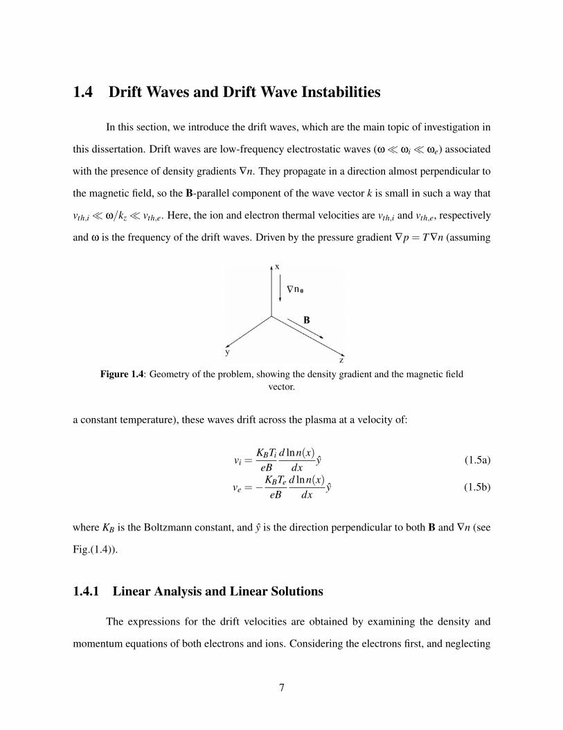
Figure 1.4: Geometry of the problem, showing the density gradient and the magnetic fieldvector.
a constant temperature), these waves drift across the plasma at a velocity of:
vi =KBTi
eBd lnn(x)
dxy (1.5a)
ve =−KBTe
eBd lnn(x)
dxy (1.5b)
where KB is the Boltzmann constant, and y is the direction perpendicular to both B and ∇n (see
Fig.(1.4)).
1.4.1 Linear Analysis and Linear Solutions
The expressions for the drift velocities are obtained by examining the density and
momentum equations of both electrons and ions. Considering the electrons first, and neglecting
7
their inertia in the parallel direction, we obtain the Boltzmann isothermal relation from the
momentum equation:∂ lnne
∂z≈ e
KBTe
∂φ
∂z(1.6)
or
ne = n0(x)exp[eφ/KBTe] (1.7)
The quasistatic process described by eq.(1.7) shows how the electrons respond instanta-
neously to the drift waves, moving almost spontaneously from a wave crest to a wave trough to
establish an equilibrium in the parallel direction. As for the ions, their velocity perpendicular to
the magnetic field is approximated by the E×B drift: ui =z×∇φ
B , where the electrostatic potential
E =−∇φ is introduced. The ion continuity equation then becomes:
∂ni
∂t+∇.(
z×∇φ
Bni) = 0 (1.8)
Keeping in mind the quasi-neutrality condition ne ≈ ni, combining eq.(1.7) and eq.(1.8) gives:
∂φ
∂t− KBTe
e∇φ× z
B.∇n0(x)n0(x)
= 0 (1.9)
Note that, for a plasma with constant magnetic field B, the ion perpendicular motion
is incompressible since ∇.(∇φ×B) = 0. The plasma fluctuations are thus associated with
variations in the density profile, as the ions move in and out along a density gradient taken in
the x-direction according to fig.(1.4). In order to obtain the corresponding dispersion relation
of these perturbations, we write the fluctuating electric potential as: φ = φ0(x)exp(iωt + ikyy),
where ω and ky are the frequency and the wavenumber of the corresponding turbulent mode.
From eq.(1.9), we obtain:
ω = ω? = uDe(x)ky (1.10)
8
where the electron diamagnetic velocity in the x direction is:
uDe(x) =−KBTe
eB.∇n0(x)n0(x)
(1.11)
Eq.(1.10) is a dispersion relation with only a real component. Therefore, it describes a
local and stable drift wave fluctuation. This peculiar result is a consequence of ignoring the ion
inertia in both parallel and perpendicular directions, which makes eq.(1.9) linear in φ(x) although
no linearization assumptions were actually made.
A general form of the dispersion relation is obtained by keeping the ion inertia in the
momentum equation for cold ions:
M(∂ui
∂t+ui.∇ui) = e(−∇φ+ui×B) (1.12)
The perpendicular ion velocity is then:
ui⊥ =−∇φ× zB− M
eB2 [∂
∂t(ui×B)+ui.∇(u×B)] (1.13a)
=−∇φ× zB− M
eB2
[∂
∂t− 1
B∇φ× z.∇
]∇⊥φ (1.13b)
The first term in eq.(1.13) represents the lowest order E×B drift. The second term represents the
ion polarization drift that makes ∇.ui 6= 0. The parallel component of the momentum equation
remains:
M(∂ui‖∂t
+ui.∇ui‖) =−e∂φ
∂z(1.14)
Using the quasi-neutrality condition ne ≈ ni, and assuming isothermal Boltzmann electrons, we
obtain the following nonlinear equation in φ(x):
∂φ
∂t+
KBTe
e∇.u+u.∇φ+
KBTe
en0(x)dn0(x)
dxu.x = 0 (1.15)
9
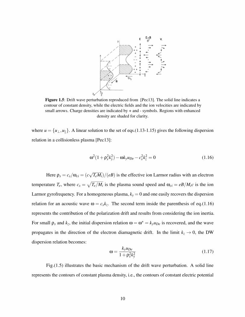
Figure 1.5: Drift wave perturbation reproduced from [Pec13]. The solid line indicates acontour of constant density, while the electric fields and the ion velocities are indicated bysmall arrows. Charge densities are indicated by + and - symbols. Regions with enhanced
density are shaded for clarity.
where u = u⊥,u‖. A linear solution to the set of eqs.(1.13-1.15) gives the following dispersion
relation in a collisionless plasma [Pec13]:
ω2(1+ρ
2s k2
y)−ωkyuDe− c2s k2
z = 0 (1.16)
Here ρs = cs/ωci = (c√
TeMi)/(eB) is the effective ion Larmor radius with an electron
temperature Te, where cs =√
Te/Mi is the plasma sound speed and ωci = eB/Mic is the ion
Larmor gyrofrequency. For a homogeneous plasma, ky = 0 and one easily recovers the dispersion
relation for an acoustic wave ω = cskz. The second term inside the parenthesis of eq.(1.16)
represents the contribution of the polarization drift and results from considering the ion inertia.
For small ρs and kz, the initial dispersion relation ω = ω? = kyuDe is recovered, and the wave
propagates in the direction of the electron diamagnetic drift. In the limit kz → 0, the DW
dispersion relation becomes:
ω =kyuDe
1+ρ2s k2
y(1.17)
Fig.(1.5) illustrates the basic mechanism of the drift wave perturbation. A solid line
represents the contours of constant plasma density, i.e., the contours of constant electric potential
10
(because of the Boltzmann equilibrium relation). When the polarization drift induced by the ion
inertia is neglected, the ion drift velocities are approximated to the lowest order by the E×B drift.
If the electric fields were steady, ions would drift with the local E×B velocity. However, because
of the fluctuating density, the plasma electric potential, and thus, the corresponding electric
field E are also fluctuating. Since E fluctuates in the y direction, ions are accelerated in the
x-direction, and their lowest order velocity is equal to vx = Ey/B =−ikyφ/B. The corresponding
dispersion relation is then that given by eq.(1.10). Because eq.(1.10) gives a non-imaginary
frequency: ω = kyuDe, there is no growth rate associated with such waves, which are considered
to be inherently stable.
To see how drift waves become unstable, one must realize that the ion drift velocity is
not really equal to the E×B drift, and that there are corrections due to the ion polarization drift.
When accounting for this additional drift, the electric potential lags the density fluctuations,
forcing ui to be outward where the plasma has already been shifted outward, and causing the
perturbations to grow. Without this polarization drift, n and φ would simply be 90 out of phase
and the motion of the waves would be purely diffusive [Che84]. An analytical derivation of
the corresponding dispersion relation for a drift wave instability is obtained by considering the
effects of the parallel plasma resistivity on the electron adiabatic response. Because the plasma
current is divergence free:
∇. j = ∇⊥. j⊥+∇‖. j‖ = 0
the perpendicular ion polarization drift will necessarily affect the electron parallel response via
the parallel plasma resistivity η‖. When writing the density and momentum equations for both
electrons and ions, it is essential to consider the momentum exchange terms that result from
electron-ion collisions. Such terms are directly proportional to the electron collision frequency
νei. An analytical derivation by [HW83] shows that the electron linear response is no longer
11
adiabatic, but rather equal to:nn0
=eφ
KBTe
ω?+ ibσ‖ω+ ibσ‖
(1.18)
where we have used the conventional notation b = ρ2s k2⊥ and σ‖ = (k2
z/k2y)(ωceωci/νei). The
density n0 is the average plasma density used as a normalization constant. Proceeding as above,
the linear dispersion relation that describes the evolution of the drift wave perturbation is equal
to:
ω2 + iσ‖
(ω(1+b)−ω
?)= 0 (1.19)
This quadratic equation bears a damped solution:
ωdamped =12
(− iσ‖(1+b)−
√4iσ‖ω?−σ2
‖(1+b)2)
(1.20)
as well as an unstable solution that describes the character of a drift wave instability:
ωunstable =12
(− iσ‖(1+b)+
√4iσ‖ω?−σ2
‖(1+b)2)
(1.21)
The analysis used to derive the previous dispersion relations was a linear analysis that
remains valid only for waves with small amplitudes. Moreover, two approximations were made
to derive these linear equations: the assumption of quasi-neutrality (plasma approximation) and
the omission of ion polarization drifts (ion inertia) in certain cases. The relaxation of these two
assumptions leads to weakly nonlinear physics described by the Hasegawa-Mima (HM) equation
and the nonlinear Hasegawa-Wakatani (HW) equations. In the following subsections, we relax
these two approximations, and perform a nonlinear analysis to get the corresponding dispersion
relation.
12
1.4.2 Hasegawa-Mima Equation
The Hasegawa-Mima equation describes a turbulent plasma regime where time scales are
fast (ω−1ci ∂/∂t 1), and parallel distance scale is long. Using this ordering, the perpendicular
ion velocity is still given by eq.(1.13), and the nonlinear equation for φ(x), i.e., eq.(1.15) is
re-written as:
∂φ
∂t− KBTe
e.∇⊥φ× z
B.∇⊥ lnn0−
c2s
ω2ci
(∂
∂t− ∇⊥φ× z
B.∇⊥
)∇
2⊥φ = 0 (1.22)
The previous equation is known as the Hasegawa-Mima equation. Upon normalization, it
becomes:∂
∂t
(∇
2⊥φ−φ
)+ z×∇⊥φ.∇⊥
(∇
2⊥φ
)−β
∂φ
∂y= 0 (1.23)
where the constant β = −d lnn0/dx measures the electron diamagnetic drift. The notation is
eased by introducing the Poisson brackets: f ,g= ∂x f ∂yg−∂xg∂y f , giving the final form of
the Hasegawa-Mima equation:
∂
∂t
(∇
2⊥φ−φ
)−β
∂φ
∂y+φ,∇2
⊥φ= 0 (1.24)
In its linear form, the Poisson brackets are dropped from the (HM) equation which becomes:
∂
∂t
(∇
2⊥φ−φ
)−β
∂φ
∂y= 0 (1.25)
The corresponding linear dispersion relation is then obtained as: ω = βky/(1+ k2⊥) = ω?/(1+
k2⊥). This is the same dispersion relation given by eq.(1.17).
13
1.4.3 Hasegawa-Wakatani Equations
A self-evident restriction of the Hasegawa-Mima equation is that it describes linearly
stable waves or fluctuations, i.e. any perturbation has to be imposed initially. This feature
violates the basic property of drift waves being unstable. The Hasegawa-Mima equation can
however readily be generalized to include this feature. For a divergence free electric current:
∇.J = 0 =⇒ ∇⊥.J⊥,i =−∇‖.J⊥,e. Here the perpendicular current driven by the ions is balanced
in the parallel direction by the electrons motion. The ion velocity is equal to:
v⊥,i =E×B
B2 − 1ωciB
d∇⊥φ
dt+
µii
ωciB∇
2(∇⊥φ) (1.26)
where an ion viscosity term µii has been added. Noting the plasma average density and resistivity
as n0 and η respectively:
∇⊥J⊥,i = en0∇⊥v⊥,i = en0∇⊥
[− 1
ωciBd∇⊥φ
dt+
µii
ωciB∇
2(∇⊥φ)]
In a similar way:
−∇‖J‖,e =−en0∇‖ve =−Te
ηe∇
2‖(
nn0− eφ
Te),
therefore:1
ωciB
[d∇2⊥φ
dt−µii∇
2(∇2⊥φ)]=
Te
ηe2n0∇
2‖(
nn0− eφ
Te) (1.27)
The electron continuity equation on the other hand gives: dn/dt +n∇.v = 0 or:
ddt
[lnn0 +
nn0
]=
Te
e2n0η∇
2‖
[ nn0− eφ
Te
](1.28)
A normalization of the time scale, the plasma density, and the plasma electric potential
14
by the ion cyclotron frequency t = ωcit, the average density: n = n/n0, and χ = eφ/Te gives:
dndt
+β∂χ
∂y=
Te
e2n0η
∂2
∂z2 (n−χ) (1.29a)
d∇2⊥χ
dt=
Te
e2n0η
∂2
∂z2 (n−χ)+µii∇4χ (1.29b)
The two previous equations constitute the Hasegawa- Wakatani (HW) equations. When linearized,
the Haseawa-Wakatani equations become:
∂n∂t
+β∂χ
∂y=
Te
e2n0η
∂2
∂z2 (n−χ) (1.30a)
∂∇2⊥χ
dt=
Te
e2n0η
∂2
∂z2 (n−χ)+µii∇4χ (1.30b)
By Fourier transform, it is readily shown that eq.(1.30a) reproduces eq.(1.18), and that the linear
dispersion relation is given by eq.(1.19)
1.5 The Drift Wave- Zonal Flow Relation
The results of the previous section show that, under certain conditions, drift waves can
become unstable. As the levels of turbulence inside the plasma increase, transport of particle
and energy is enhanced, and confinement is easily destroyed. Fortunately, the mechanism
of turbulence regulation via self-generation and amplification of zonal flows (ZFs) [DIIH05,
FII+04].
Formation of zonal flows is a well-known and well-documented phenomenon in 2D
turbulent systems [DIIH05]. In contrast to 3D turbulent systems, vortex stretching is inhibited
in 2D systems, and turbulence is characterized by an inverse energy cascade in which energy
is transferred to large spatial structures. In the inertial range, a direct enstrophy cascade where
turbulent energy is driven to smaller scales dominates. The turbulent energy is then dissipated
15
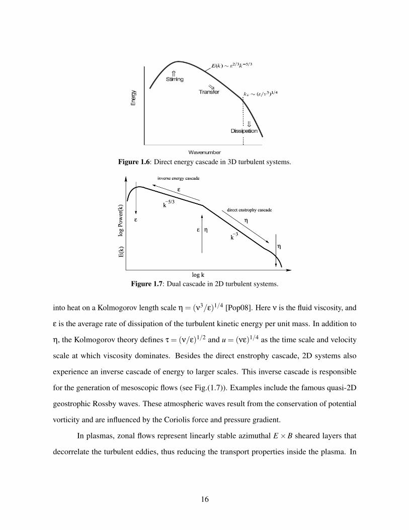
Figure 1.6: Direct energy cascade in 3D turbulent systems.
Figure 1.7: Dual cascade in 2D turbulent systems.
into heat on a Kolmogorov length scale η = (ν3/ε)1/4 [Pop08]. Here ν is the fluid viscosity, and
ε is the average rate of dissipation of the turbulent kinetic energy per unit mass. In addition to
η, the Kolmogorov theory defines τ = (ν/ε)1/2 and u = (νε)1/4 as the time scale and velocity
scale at which viscosity dominates. Besides the direct enstrophy cascade, 2D systems also
experience an inverse cascade of energy to larger scales. This inverse cascade is responsible
for the generation of mesoscopic flows (see Fig.(1.7)). Examples include the famous quasi-2D
geostrophic Rossby waves. These atmospheric waves result from the conservation of potential
vorticity and are influenced by the Coriolis force and pressure gradient.
In plasmas, zonal flows represent linearly stable azimuthal E ×B sheared layers that
decorrelate the turbulent eddies, thus reducing the transport properties inside the plasma. In
16
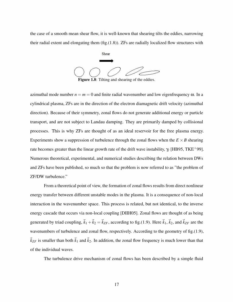
the case of a smooth mean shear flow, it is well-known that shearing tilts the eddies, narrowing
their radial extent and elongating them (fig.(1.8)). ZFs are radially localized flow structures with
Figure 1.8: Tilting and shearing of the eddies.
azimuthal mode number n = m = 0 and finite radial wavenumber and low eigenfrequency ω. In a
cylindrical plasma, ZFs are in the direction of the electron diamagnetic drift velocity (azimuthal
direction). Because of their symmetry, zonal flows do not generate additional energy or particle
transport, and are not subject to Landau damping. They are primarily damped by collisional
processes. This is why ZFs are thought of as an ideal reservoir for the free plasma energy.
Experiments show a suppression of turbulence through the zonal flows when the E×B shearing
rate becomes greater than the linear growth rate of the drift wave instability, γl [HB95, TKE+99].
Numerous theoretical, experimental, and numerical studies describing the relation between DWs
and ZFs have been published, so much so that the problem is now referred to as ”the problem of
ZF/DW turbulence.”
From a theoretical point of view, the formation of zonal flows results from direct nonlinear
energy transfer between different unstable modes in the plasma. It is a consequence of non-local
interaction in the wavenumber space. This process is related, but not identical, to the inverse
energy cascade that occurs via non-local coupling [DIIH05]. Zonal flows are thought of as being
generated by triad coupling,~k1 +~k2 =~kZF , according to fig.(1.9). Here~k1,~k2, and~kZF are the
wavenumbers of turbulence and zonal flow, respectively. According to the geometry of fig.(1.9),
~kZF is smaller than both~k1 and~k2. In addition, the zonal flow frequency is much lower than that
of the individual waves.
The turbulence drive mechanism of zonal flows has been described by a simple fluid
17
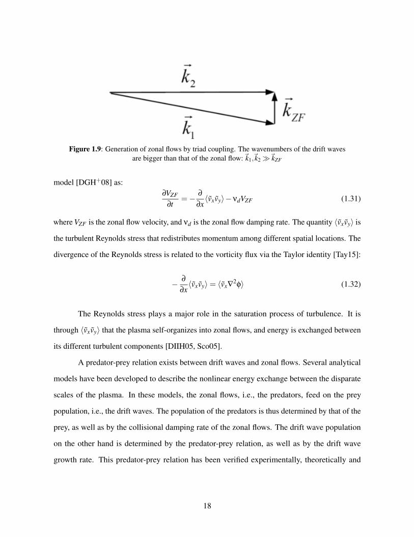
Figure 1.9: Generation of zonal flows by triad coupling. The wavenumbers of the drift wavesare bigger than that of the zonal flow:~k1,~k2~kZF
model [DGH+08] as:∂VZF
∂t=− ∂
∂x〈vxvy〉−νdVZF (1.31)
where VZF is the zonal flow velocity, and νd is the zonal flow damping rate. The quantity 〈vxvy〉 is
the turbulent Reynolds stress that redistributes momentum among different spatial locations. The
divergence of the Reynolds stress is related to the vorticity flux via the Taylor identity [Tay15]:
− ∂
∂x〈vxvy〉= 〈vx∇
2φ〉 (1.32)
The Reynolds stress plays a major role in the saturation process of turbulence. It is
through 〈vxvy〉 that the plasma self-organizes into zonal flows, and energy is exchanged between
its different turbulent components [DIIH05, Sco05].
A predator-prey relation exists between drift waves and zonal flows. Several analytical
models have been developed to describe the nonlinear energy exchange between the disparate
scales of the plasma. In these models, the zonal flows, i.e., the predators, feed on the prey
population, i.e., the drift waves. The population of the predators is thus determined by that of the
prey, as well as by the collisional damping rate of the zonal flows. The drift wave population
on the other hand is determined by the predator-prey relation, as well as by the drift wave
growth rate. This predator-prey relation has been verified experimentally, theoretically and
18
numerically [DIIH05, MRS09].
1.6 The Drift Wave-Axial Flow Relation
In addition to the drift wave-zonal flow relation, theoretical studies supported by ex-
perimental results reveal a similar relation between drift waves and the axial (parallel) flows
in both toroidal and linear plasmas [KIIe5, KIK+16, IKI+16]. Measurements from Alcator
C-Mod tokamak show that the observed intrinsic flow is proportional to the edge temperature
gradient [RHD+11]. The plasma behaves like a heat engine that uses the free energy to produce
an intrinsic flow. During this process, the temperature gradient excites turbulence, which not
only relaxes ∇T , but also drives a non-diffusive residual stress [KDG10]. In a similar vein,
measurements from PANTA linear device show a direct relation between the parallel Reynolds
stress and the parallel flows. These axial flows play an important role in stabilizing the plasma
and reducing certain MHD and resistive wall modes, particularly in large scale fusion devices
where parallel momentum injection via external Neutral Beam Injections (NBIs) is thought
to be insufficient on its own. The aforementioned experimental observations were explained
by theoretical investigations, which attribute an essential role to the parallel Reynolds stress
〈vxvz〉 in accelerating the formation of axial flows [DMG+09, KJD+11, DKG+13]. Similar to
the perpendicular Reynolds stress, the parallel Reynolds stress redistributes the momentum in
the parallel direction, and uses the ∇n free energy to accelerate vz. Specifically, it is the presence
of a non-zero parallel residual stress Πresxz = Πres
xz (∇n,∇Te) when the parallel symmetry is broken
that triggers the generation and acceleration of vz. The parallel residual stress is the counterpart
of the poloidal residual stress that accelerates the zonal flows. Experiments on TJ-II stellarator
confirm the existence of a significant turbulent residual parallel stress that produces a toroidal
intrinsic torque. An electrode biasing experiment on J-TEXT achieved a nearly zero toroidal
rotation profile, thereby showing that the intrinsic torque can be explained by the measured
19
residual stress [GmcHP+06]. Recently, a gyrokinetic simulation also predicted that the residual
stress generates the intrinsic torque, which is consistent with the measured rotation profile in
DIII-D [WGE+17].
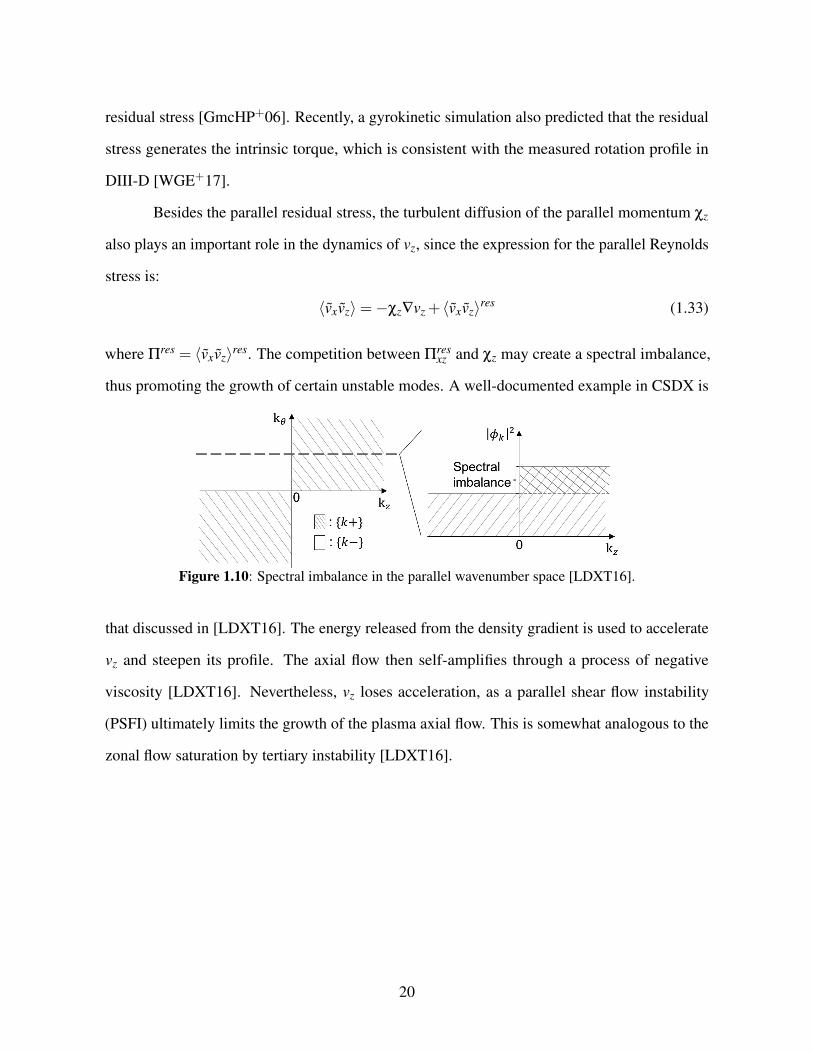
Besides the parallel residual stress, the turbulent diffusion of the parallel momentum χz
also plays an important role in the dynamics of vz, since the expression for the parallel Reynolds
stress is:
〈vxvz〉=−χz∇vz + 〈vxvz〉res (1.33)
where Πres = 〈vxvz〉res. The competition between Πresxz and χz may create a spectral imbalance,
thus promoting the growth of certain unstable modes. A well-documented example in CSDX is
Figure 1.10: Spectral imbalance in the parallel wavenumber space [LDXT16].
that discussed in [LDXT16]. The energy released from the density gradient is used to accelerate
vz and steepen its profile. The axial flow then self-amplifies through a process of negative
viscosity [LDXT16]. Nevertheless, vz loses acceleration, as a parallel shear flow instability
(PSFI) ultimately limits the growth of the plasma axial flow. This is somewhat analogous to the
zonal flow saturation by tertiary instability [LDXT16].
20
1.7 Dissertation Outline
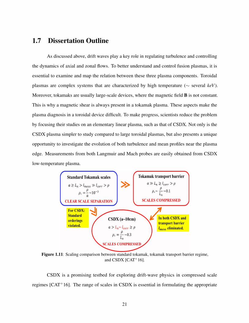
As discussed above, drift waves play a key role in regulating turbulence and controlling
the dynamics of axial and zonal flows. To better understand and control fusion plasmas, it is
essential to examine and map the relation between these three plasma components. Toroidal
plasmas are complex systems that are characterized by high temperature (∼ several keV ).
Moreover, tokamaks are usually large-scale devices, where the magnetic field B is not constant.
This is why a magnetic shear is always present in a tokamak plasma. These aspects make the
plasma diagnosis in a toroidal device difficult. To make progress, scientists reduce the problem
by focusing their studies on an elementary linear plasma, such as that of CSDX. Not only is the
CSDX plasma simpler to study compared to large toroidal plasmas, but also presents a unique
opportunity to investigate the evolution of both turbulence and mean profiles near the plasma
edge. Measurements from both Langmuir and Mach probes are easily obtained from CSDX
low-temperature plasma.
Figure 1.11: Scaling comparison between standard tokamak, tokamak transport barrier regime,and CSDX [CAT+16].
CSDX is a promising testbed for exploring drift-wave physics in compressed scale
regimes [CAT+16]. The range of scales in CSDX is essential in formulating the appropriate
21
physical models used to describe turbulence and flow dynamics as shown in figure (1.11). Note
that in CSDX, the normalized radius ρ? = ρ/a is comparable to that in H-mode edge transport
barrier regimes. Moreover, the mesoscopic length lmeso is eliminated from the scale ordering in
CSDX. This shows why CSDX is a useful venue, where studies of scale compression can be
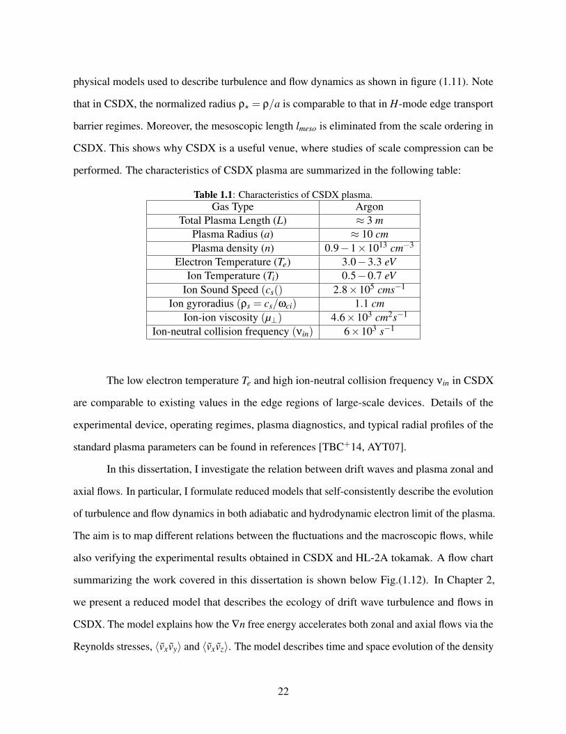
performed. The characteristics of CSDX plasma are summarized in the following table:
Table 1.1: Characteristics of CSDX plasma.Gas Type Argon
Total Plasma Length (L) ≈ 3 mPlasma Radius (a) ≈ 10 cmPlasma density (n) 0.9−1×1013 cm−3
Electron Temperature (Te) 3.0−3.3 eVIon Temperature (Ti) 0.5−0.7 eV
Ion Sound Speed (cs() 2.8×10⁵ cms−1
Ion gyroradius (ρs = cs/ωci) 1.1 cmIon-ion viscosity (µ⊥) 4.6×103 cm2s−1
Ion-neutral collision frequency (νin) 6×10³ s−1
The low electron temperature Te and high ion-neutral collision frequency νin in CSDX
are comparable to existing values in the edge regions of large-scale devices. Details of the
experimental device, operating regimes, plasma diagnostics, and typical radial profiles of the
standard plasma parameters can be found in references [TBC+14, AYT07].
In this dissertation, I investigate the relation between drift waves and plasma zonal and
axial flows. In particular, I formulate reduced models that self-consistently describe the evolution
of turbulence and flow dynamics in both adiabatic and hydrodynamic electron limit of the plasma.
The aim is to map different relations between the fluctuations and the macroscopic flows, while
also verifying the experimental results obtained in CSDX and HL-2A tokamak. A flow chart
summarizing the work covered in this dissertation is shown below Fig.(1.12). In Chapter 2,
we present a reduced model that describes the ecology of drift wave turbulence and flows in
CSDX. The model explains how the ∇n free energy accelerates both zonal and axial flows via the
Reynolds stresses, 〈vxvy〉 and 〈vxvz〉. The model describes time and space evolution of the density
22
n, the azimuthal and axial flows vy and vz, and the turbulent energy ε = 〈n2 + v2y + v2
z/2〉. The
model explains how the Reynolds stresses redistribute the momentum in the axial and azimuthal
directions. It also relates parallel to perpendicular flow dynamics by introducing a coupling
constant σvT . This constant measures the degree of parallel symmetry breaking, as well as the
correlator 〈kmkz〉, which is at the essence of the parallel residual stress. Chapter 2 presents a
complete picture of the different interactions that occur between turbulence and mean profiles,
including a detailed study of feedback loops that exist between different elements of the plasma.
In Chapter 3, I focus on the DW/ZF relation. A numerical validation and verification
of the turbulence regulation phenomenon in CSDX is presented. This turbulence regulation
has been observed experimentally in references [CTD+15, CAT+16]. For this purpose, another
reduced model that describes space and time evolution of n and vy, in addition to the usual
potential enstrophy ε = 〈(n−∇2φ)2/2〉 is formulated. Chapter 3 focuses only on the DW/ZF
relation in the adiabatic electron limit. It presents numerical results that describe the evolution of
the plasma mean and turbulent profiles, as the magnitude of the magnetic field B is varied. In
addition, a new criterion for turbulence saturation is established. This criterion is characterized by
the dimensionless quantity RDT , which compares the production rate of the turbulent enstrophy
due to the relaxation of the mean profiles, to the destruction rate of ε via coupling to the mean
flow because of the predator-prey relation.
Chapter 4 examines the relation between DWs and ZFs is examined in another plasma
limiting case, known as the hydrodynamic limit. In this case, the equations that describe the
behavior of the plasma density and vorticity decouple, and are essentially reduced to a 2D
Navier-Stokes equation. In contrast to the adiabatic limit, zonal flows are shown to collapse
in the hydrodynamic limit, and turbulence is enhanced instead of being suppressed. These
changes in the plasma dynamics are interpreted from a zonal flow production perspective. As
the adiabaticity parameter decreases, the particle transport increases, while the efficiency of
plasma zonal flows production decreases. The edge shear layer weakens, the thermal confinement
23
degrades, and an MHD activity is eventually triggered. This chapter is of particular interest in the
context of understanding the enhancement of turbulence and the collapse of the edge shear layer
in density limit experiments - a topic of crucial importance for future magnetic fusion devices.
Lastly, Chapter 5 summarizes the findings of this dissertation, points to future work on
the relation between turbulence and mean flows, and presents a list of potential experiments and
recommendations to further advance the experiments of this study.
24
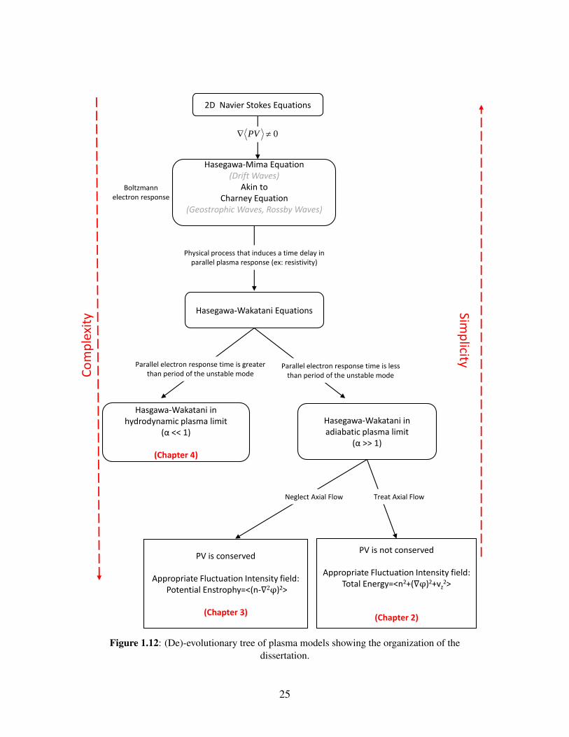
2D Navier Stokes Equations
Hasegawa-Mima Equation (Drift Waves)
Akin toCharney Equation
(Geostrophic Waves, Rossby Waves)
Boltzmann electron response
0 PV
Physical process that induces a time delay in parallel plasma response (ex: resistivity)
Hasegawa-Wakatani Equations
Parallel electron response time is greater than period of the unstable mode
Hasgawa-Wakatani in hydrodynamic plasma limit
(α << 1)
(Chapter 4)
PV is conserved
Appropriate Fluctuation Intensity field:Potential Enstrophy=<(n-∇2φ)2>
(Chapter 3)
Parallel electron response time is less than period of the unstable mode
Hasegawa-Wakatani in adiabatic plasma limit
(α >> 1)
Neglect Axial Flow
PV is not conserved
Appropriate Fluctuation Intensity field: Total Energy=<n2+(∇φ)2+vz
2>
(Chapter 2)
Treat Axial Flow
Co
mp
lexi
ty
Simp
licity
Figure 1.12: (De)-evolutionary tree of plasma models showing the organization of thedissertation.
25
Chapter 2
THE ECOLOGY OF FLOWS AND
DRIFT WAVE TURBULENCE IN CSDX:
A MODEL
2.1 INTRODUCTION
Drift wave (DW) turbulence is one of the fundamental issues in magnetically confined
plasmas, and continues to be a subject of interest for many experimental and theoretical stud-
ies [Ter00, DIIH05]. Driven by radial inhomogeneities, drift wave fluctuations increase the
turbulent transport of particles and energy, which leads ultimately to loss of the plasma particles,
heat, etc. One mechanism that regulates these fluctuations is the self-generation and amplification
of sheared E×B flows by turbulent stresses. This is related, but not identical to the inverse energy
cascade in a two-dimensional fluid that occurs via local coupling in the wavenumber space. Here,
the generation of zonal (azimuthal) flows occurs through non-local nonlinear energy transfer
between the small and large scales of the plasma [Hor99, Sco05, MRS09]. Such flows play an
important role in saturating the drift wave instabilities, in L−H transition, and in the formation
26
of internal transport barriers (ITBs) [KD03]. Drift wave turbulence is also responsible for the
generation of toroidal/axial flows, which play a crucial role in the macrostability of fusion grade
tokamak plasmas. In particular, intrinsic toroidal flows are needed in large scale devices, where
momentum input through NBI is not effective. Such flows stabilize some MHD and resistive wall
modes, suppress turbulence, and enhance the overall particle confinement [KJD+11, GTA+99].
The relationship between drift waves and zonal flows has been extensively studied, so
much so that the problem is now referred to as drift wave/zonal flow turbulence. Several self-
regulating predator-prey models were developed, where the drift wave fluctuations correspond to
the prey population and the zonal flows correspond to the predator population [DLCT94, II96,
IIFY99]. As the population of drift waves grows rapidly, it supports the predator population.
Zonal flows then control the drift waves by feeding on them, while being themselves regulated
by a predator-prey competition and by nonlinear damping [DIIH05]. The existing versions of
these models however, do not adequately address the problem of zonal flow saturation.
In a different vein, axial flow formation by turbulence requires a breaking in parallel
symmetry and a non-zero correlator 〈kzkm〉 = ∑m kzkm|φ|2. In tokamaks, it is (usually) the
magnetic shear that enables the parallel symmetry breaking. In linear devices however, B
is constant and standard mechanisms do not apply. Recently, a parallel symmetry breaking
mechanism that is based in drift wave turbulence and axial flow shear was developed [LDXT16].
This mechanism does not rely on complex magnetic geometry to generate a parallel residual
stress Πresxz ∝ 〈kzkm〉. The energy released from the density gradient is used to accelerate an axial
flow through a negative viscosity process. For strong flows, the parallel shear flow instability
(PSFI) controls the dynamics of vz.
Inverse energy cascade has been observed in both 2D and 3D systems [BMT12]. Ex-
amples include reversal of the flux of energy in geophysical flows subject to the Earth’s rota-
tion [MAP09], as well as in shallow fluid layers [XBFS11]. In plasmas, inverse energy cascade
that results in the generation of broadband turbulence and large scale coherent structures from
27
DW fluctuations is widely accepted now. With drift waves triggering the formation of both axial
and azimuthal flows (Fig.2.1), fundamental questions concerning the flow configuration arise:
What mechanisms regulate the self-organization process, and ordain the final configuration of
turbulence and flows in the plasma? How is energy partitioned between the fluctuations and the
different flows vz and vy in the plasma? Moreover, since fluctuations and mean flows constitute
an interdependent system, could there be a coupling relation between vy and vz? If so, what
determines the strength of this coupling? And most importantly, how does this coupling affect
the energy branching ratio in the plasma?
To answer these questions, we present in this paper a 1D (in radius) reduced k− ε type
model that describes the evolution of the three mean fields: density n, axial and azimuthal flows
vz and vy, as well as variations in the fluctuation intensity ε = 〈n2 +(∇⊥φ)2 + v2z 〉, in the linear
plasma of CSDX. The model is derived from the Hasegawa-Wakatani system with axial flow
evolution included. The model self-consistently relates variations in ε to the evolution of the
mean profiles via the particle flux 〈nvx〉, and the parallel and perpendicular Reynolds stresses
〈vxvz〉 and 〈vxvy〉. Because of parallel compression, the fluctuation intensity is the relevant
conserved field.
To explain the relation between vy and vz with respect to ε, the model uses a mixing
length lmix that reflects turbulence suppression by the axial and azimuthal flow shear. External
particle and axial flow sources which result from injection of neutrals and axial momentum, are
included in this model. When the work done by the fluctuations on the parallel flow is less than
that done on the perpendicular flow, the model can be reduced to a 2-field predator-prey model,
where the azimuthal flow feeds on the density population.
The model is a necessary intermediary between a 0D model that shows the structure of
the flows and fluctuations, and a full DNS. For a multiscale system such as CSDX, a reduced
model provides a route to an interpretation of the experimental results, and gives detailed insight
into the feedback loops between the disparate scales. At the same time, it avoids the labor of
28
Linear Dissipation and Saturation
Drift Wave
Turbulence
Zonal Flows
Axial Flows
Relation ?
Limited by PSFI
∇n free energy
Feedback Loop 1
Feedback Loop 2
Figure 2.1: A schematic of the ecology of drift wave turbulence, zonal, and axial flows. Thefirst feedback loop relates the drift waves to the zonal flows via 〈vxvy〉. A second feedback loop
exists as a result of a potential relation between vy and vz. The second loop relates thefluctuations to both mean flows.
a full DNS. The model consists of a set of compact equations that describe the evolution of
the plasma stresses and flows. It shows how ∇n free energy accelerates both vy and vz, and
investigates the coupling relation between the parallel and perpendicular flow dynamics in CSDX
by introducing σV T , the empirical measure of the acoustic coupling in the plasma.
The 1D reduced model description taken here should provide a useful new interme-
diate approach for the simulation of self-consistent evolution edge and SOL plasma profiles,
transverse and parallel flows and turbulence, and would allow the study of main plasma and
29
trace impurity dynamics across timescales ranging from a few turbulent correlation times up to
system equilibrium timescales. When modified to include toroidal and open-field line effects,
and extended to a 2D geometry along the magnetic field and binormal directions, our proposed
reduced model would bridge the gap between existing time-averaged fluid codes of the edge and
SOL region of confinement devices (see e.g. ref.[WRK+15]) which are incapable of capturing
such self-consistent dynamical phenomena, and fully turbulent direct numerical simulations
(see e.g. refs. [TGT+10, RMRP92]) which capture self-consistent profile and flow evolution but
are computationally expensive and thus difficult to use for long time scale dynamical evolution
studies. Such a new capability might be useful to study the self-consistent entrainment and
transport of eroded wall impurities in flowing edge and SOL plasma and the long-time migration
of these materials in the SOL and divertor regions of confinement devices. These obvious
extensions are left as future work.
The rest of the paper is organized as follows. Section 2.2 presents the structure of the
model, as well as a full derivation of the involved equations and an interpretation of each term of
these equations. Section 2.3 elaborates on the relation between drift waves and zonal flows, and
calculates the turbulent expressions for the particle flux and the vorticity flux. Expressions for the
perpendicular Reynolds stress and the Reynolds work are also presented. Section 2.4 is dedicated
to the parallel Reynolds stress. This sections explains how drift waves accelerate the axial flows
through 〈vxvz〉. An empirical constant σV T is introduced in this section. By analogy to pipe
flows, σV T is presented as a measure of the acoustic coupling or the efficiency of converting the
∇n energy to drive an axial flow. σV T is then used to establish a direct relation between the axial
and the azimuthal flow shear, as both residual stresses Πresxy and Πres
xz are proportional to ∇n. An
expression for the mixing length lmix that depends on both shears is derived in section 2.5. In
section 2.6, we give a summary and a discussion of the model, before reducing it to a 2-field
predator-prey model in section 2.7. Finally, conclusion and discussion are given in section 4.8.
30
2.2 THE MODEL AND ITS STRUCTURE
The basic equations are derived from the Hasegawa-Wakatani system [HW83, HW87],
with axial flow velocity vz evolution included. In a box of dimensions: 0≤ x≤ Lx, 0≤ y < Ly
and 0≤ z≤ Lz, and for a straight magnetic field B = Bz, these equations are [LD17]:
dndt
+vE .∇〈n〉+n0∇zvz =−v2
thνei
∇2z (φ− n)+D0∇
2⊥n+n, φ (2.1a)
d∇2⊥φ
dt+vE .∇〈∇2
⊥φ〉=−v2
thνei
∇2z (φ− n)+µ0∇
4⊥φ−νin(vy− vn)+∇2
⊥φ, φ (2.1b)
dvz
dt+vE .∇〈vz〉=−c2
s ∇zn+ν0∇2⊥vz−νin(vz− vn)+vz, φ (2.1c)
Here x, y and z are the radial, azimuthal and axial directions respectively. The fields
are normalized as follows: n≡ ne/n0, φ≡ eφ/Te, t ≡ ωcit, vz ≡ vz/cs and length≡ length/ρs.
n0 and Te are the average density and electron temperature respectively, ωci = eB/mi is the ion
cyclotron frequency, cs =√
Te/mi is the ion sound speed and ρs = cs/ωci is the ion Larmor
radius with temperature Te. vth and νei are the electron thermal velocity and the electron-ion
collision frequency, respectively. The total time derivative is: d/dt = ∂t +vE .∇, and the axial
ion pressure gradient is neglected in the vz equation. The neutral friction, proportional to the ion-
neutral collision frequency νin = nn√
8Ti/πmi, is a natural sink for energy that inverse cascades
to larger scales. This friction is especially significant near the plasma boundary. Its expression
can be further simplified by taking vn ≈ 0 close to the boundary. Terms that are proportional
to D0, µ0 and ν0 dissipate energy via viscous collisions. Finally, the nonlinear advection terms
are expressed as Poisson brackets: f ,g= ∂x f ∂yg−∂xg∂y f , and represent spatial scattering of
fluctuations.
The system of eqs.(2.1) describes a variety of linearly unstable modes. One eigenmode
of this system is the strongly damped ion drift wave with an eigenfrequency that satisfies the
31
relation: |ω| < |kzcs|. Here kz is the parallel wave number. Such a wave is heavily damped,
will be difficult to excite, and thus will not be considered here. A second solution to this
system describes the dynamics of the parallel shear flow instability (PSFI). The PSFI describes
turbulence production due to free energy released from parallel flow shear [KIK+16, KII16]. In
contrast to other linear plasmas [KIIe5, IKI+16], experimental results from the CSDX linear
device show that the parallel flow shear v′z is well below the critical threshold necessary to drive
PSFI [LD17]. The PSFI is thus heavily damped in CSDX, and will also not be considered here.
A third solution describes the dynamics of the coupled 3D drift-ion acoustic turbulence. In
this paper, we are mainly concerned with the coupling between the parallel and perpendicular
flow dynamics. Thus we focus only on the dynamics of the coupled drift-ion acoustic waves.
We decompose each field into a mean and a fluctuating part: f = 〈 f 〉+ f (x,y,z, t), where the
averaging is performed over the directions of symmetry y and z:
f (x, t) = 〈 f (x, t)〉= 1LzLy
∫ Lz
0dz
∫ Ly
0dy f (x,y,z, t)
where we assume that the plasma profiles do not change substantially along the axial direction.
In the presence of compressible parallel flows, conservation of potential vorticity (PV) -
and thus that of the potential enstrophy - is broken. Coupling between the PV fluctuations and
the parallel flow compression thus defines an energy transfer channel between the parallel and
perpendicular flow dynamics. This energy exchange influences the wave momentum density and
modifies the zonal momentum balance theorem [WDH12]. In its new form, the zonal momentum
balance theorem shows that coupling between drift-acoustic waves acts as a driving source that
allows stationary turbulence to excite zonal flows in the absence of any driving force or potential
enstrophy flux. The coupling drive involves both perpendicular and parallel dynamics, and does
not require symmetry breaking in the turbulence spectrum. Therefore, instead of using potential
32
enstrophy as the fluctuation intensity field, we use the mean fluctuation energy 〈ε〉 defined as:
〈ε〉= 1LzLy
L‖∫0
dz2π∫
0
dθε(r) =1
LzLy
∫ Lz
0dz
∫ Ly
0dyε(x) =
⟨n2 +(∇⊥φ)2 + v2
z⟩
2,
where z and y are the axial (parallel) and azimuthal (perpendicular) directions respectively, and
L‖ = Lz is the axial length of the plasma. Here we assume periodicity in the axial direction z.
The mean fluctuating energy 〈ε〉, interpreted as a sum of internal energy 〈n2〉 and kinetic energy:
〈(∇⊥φ)2〉+ 〈v2z 〉, is conserved up to dissipation and internal production, as demonstrated later.
The time evolution of 〈ε〉 is:
d〈ε〉dt
=1
LzLy
∫(n
dndt
+∇⊥φd∇⊥φ
dt+ vz
dvz
dt)dydz (2.2)
An expression for eq.(2.2) is obtained by multiplying the set of eqs.(2.1) by n, −φ and vz
respectively, and integrating along the directions of symmetry to get:
〈dε
dt〉=−〈nvx〉
dndx−〈vxvy〉
dvy
dx−〈vxvz〉
dvz
dx− 1
LzLy
v2th,e
νei
∫ [∂z(Φ− n)
]2dz−〈nvz〉
−νin
(〈v2
y〉+ 〈v2z 〉)− 1
LzLy
∫ (D0(∇⊥n)2 +µ0(∇
2⊥φ)2 +ν0(∇⊥vz)
2)
dydz
+1
LzLy
∫ (nn, φ− φ∇2
⊥φ, φ+ vzvz, φ)
dydz
(2.3)
Here we have used periodic boundary conditions in the y direction to obtain the fourth
term of the RHS of eq.(2.3). The first three terms on the RHS of eq.(2.3) are direct mean-
fluctuation coupling terms. They relate the variations of ε to the variations of the mean profiles
of n, vy and vz via 〈nvx〉, 〈vxvy〉 and 〈vxvz〉.
A common issue that arises while using such reduced models is the closure problem.
To obtain equations that contain only the mean quantities, we simplify the energy equation by
examining each term of eq.(2.3), in order to properly construct the equation for ε. In the case of
33
pure drift wave turbulence, the dvz/dx term is absent and ω < ω? ∝ ∇n. The density gradient
term is then the only source of energy production. It is positive definite, and represents the rate
at which free energy is extracted from the density gradient ∇n. The second term on the RHS of
eq.(2.3) is the Reynolds power. It represents the free energy coupled to the azimuthal flow vy
via the Reynolds stress 〈vxvy〉. For pure DWs and stable Kelvin-Helmholtz (KH) modes, this
energy is transfered to the mean flow and the Reynolds power is negative. The third term, on
the other hand, can represent either an energy source or an energy sink. Depending on the sign
of the cross phase between vx and vz, this term can be either positive or negative. A detailed
discussion of this cross phase relation and of the parallel Reynolds stress is deferred to a later
section. The dissipation term −∫[∂z(Φ− n)]2dz is associated with the phase difference between
the density fluctuations n and the electric potential fluctuations φ. This term is always negative.
In the frequently encountered case of weakly non-adiabatic electrons, this term is always smaller
than the energy input source term: −∫[∂z(Φ− n)]2dz −〈nvx〉∇n [SDSK13]. Indeed, for
n = (1− i∆)φ with ∆ 1 and ω ' |ω?|/(1+ k2⊥ρ2
s ), the estimates of the dissipation and the
energy input terms are: ω2(|ω?|−ω)2 and ω|ω?|(|ω?|−ω)2 respectively. With ω < |ω?|, the
dissipation term can be neglected from eq.(2.3). The 〈nvz〉 term represents parallel particle
flux. Since such flux can be experimentally zeroed, it will be omitted from the energy equation.
Terms that are proportional to D0, µ0 and ν0, represent collisional energy dissipation by direct
energy cascade. These terms damp the fluctuation energy at small scales at a rate√
ε/lmix.
We write the energy dissipation as ε3/2/lmix, and leave the discussion of the expression for
the turbulent mixing length lmix to a subsequent section. In addition to collisional dissipation,
ion-neutral collisions represent a nonlinear energy damping to larger scales. Both collisional
dissipation and neutral energy damping represent a sink of turbulent energy ε. Finally, the
nonlinear terms in eqs. (2.1) are related to the E×B drift, the polarization drift, and the axial drift
respectively. These terms represent the spreading of turbulence. This spreading is mesoscopic,
and involves two aspects. The first aspect is a perturbation in the local intensity gradient ∂xε,
34
i.e., a diffusion of the energy envelope to a more stable region away from its source. The second
aspect includes nonlinear interaction of the local fluctuations via inverse cascade. Based in the
three wave coupling, zonal flows created through inverse cascade shear the fluctuations and
regulate turbulence spreading [GDH06, GDH07]. We write this energy spreading as a Fickian
energy flux: Γε =−Dε∂xε =−lmixε1/2∂xε. An energy source P representing drift wave turbulent
energy production is added to eq.(2.3). The generation of these fluctuations results from the
relaxation of the mean profiles and represents the excitation in the linear phase. The energy
production term is linear in ε and proportional to γε, the characteristic growth rate of the DW
instabilities: P = γεε. The final form of eq.(2.3) then becomes:
∂ε
∂t+∂xΓε =−〈nvx〉
dndx−〈vxvz〉
dvz
dx−〈vxvy〉
dvy
dx− ε3/2
lmix+P (2.4)
In addition to eq.(2.4), the equations for n, vy and vz, which form the reduced model of
turbulence intensity for the modified Hasegawa-Wakatani model are:
∂n∂t
=− ∂
∂x〈vxn〉+Dc
∂2n∂x2 +Sn (2.5)
∂vz
∂t=− ∂
∂x〈vxvz〉+νc,‖
∂2vz
∂x2 −νinvz−νiivz +Svz (2.6)
∂vy
∂t=− ∂
∂x〈vxvy〉+νc,⊥
∂2vy
∂x2 −νinvy−νiivy +Svy (2.7)
Here we assumed that the electron pressure gradient does not vary neither in the axial nor in
the azimuthal direction. Note however that this assumption remains valid only in the case of
an attached plasma. When the pressure of the injected neutral gas is high enough, a detached
plasma is obtained, and axial and azimuthal variations of ∇pe are no longer equal to zero. The
first terms on the RHS of eqs.(4.8a-2.7) represent particle and momentum transport, while those
proportional to Dc, νc,⊥ and νc,‖ represent collisional diffusivity and viscosity respectively. A
35
particle source Sn representing the ionization of the injected neutrals is added to the density
equation. Similarly, axial and azimuthal momentum sources Svz and Svy representing external
input of momentum into the plasma are added to vy and vz equations. In CSDX however, no
external momentum is injected and Svz = Svy = 0, in contrast to refs. [IKI+16, KIK+16, KII17]
where external axial momentum is injected into the plasma. In eq.(2.7), the term proportional to
the ion-neutral collision frequency νin represents momentum transfer between ions and neutrals,
and is significant only in the boundary layer close to the plasma wall. The last term proportional
to νii represents viscous damping via ion-ion collisions. The expressions for viscous and diffusive
coefficients are [LL94]:
Dc =D
1+ω2ciτ
2i' De
(ωciτi)2 ∼4√
2πn0 lnΛe2√me
3√
Te(2.8a)
νc,⊥ = νi,⊥ =310
niTi
ω2ciτi∼
2√
πn20 lnΛe2m3/2
i
T 1/2i
(2.8b)
νc,‖ = νe,‖ = 0.73neTeτe ∼3√
meT 5/2e
4√
2π lnΛe4(2.8c)
The system formed by eqs.(2.4-2.7) conserve the total energy Etot in time, up to dissipa-
tion and production. Here Etot is equal to the sum of the turbulent energy ε and the mean energy
Emean =(n2 + v2
z +(∇⊥φ)2)/2. For zero energy flux conditions at the boundaries (∂xε = 0),
energy conservation (up to dissipation and production) is demonstrated as:
d〈Etot〉dt
=d〈ε〉dt
+d〈Emean〉
dt
=d〈ε〉dt
+12
∂
∂t
∫ [n2 + v2
z +(∇⊥φ)2]dzdy
=−〈nvx〉dndx−〈vxvz〉
dvz
dx−〈vxvy〉
dvy
dx+P− ε3/2
lmix
+ 〈nvx〉dndx
+ 〈vxvz〉dvz
dx+ 〈vxvy〉
dvy
dx
=−ε3/2
lmix+P
(2.9)
36
where the order of operations .. and 〈..〉 have been interchanged. Eqs.(2.4-2.7) thus constitute a
model that describes profile evolution for both parallel and perpendicular flows, in addition to
the plasma density, by self-consistently evolving turbulence as well as the mean profiles. This
model offers the possibility to explain the generation and acceleration of intrinsic axial flows as
a result of changes in the turbulence spectrum, governed by conservation of total energy Etot .
2.3 CALCULATING THE TURBULENT FLUXES
Eqs.(2.4-2.7) describe time and space evolution of the three mean fields: n, vy and vz,
in addition to the mean fluctuating energy ε. The solution of this system of equations requires
calculating the expressions for the different turbulent fluxes in terms of ε and the mean field
gradients. In this section, we determine the expressions for the various turbulent fluxes, with the
provision that these expressions are valid only in the case of nearly adiabatic electrons, that is
when k2z v2
th/(νei|ω|) 1. In this limit, quasi-linear theory is used to calculate the expressions for
the transport fluxes by Fourier decomposing each field as: fm = δ fm(x)ei[kmy+kzz−ωt] where ω =
ωr + i|γm|, with |γm| ωrm = ω?(1+k2
⊥ρ2s )−1. Here ω? = kmvd , where the electron diamagnetic
velocity is vd =−ρscs∇n = ρscs/Ln,
2.3.1 The Turbulent Particle Flux
The particle flux 〈nvx〉 is calculated after linearizing the density equation:
∂n∂t− vxvd +∇zvz =−
v2th
νei∇
2z (φ− n)+D0∇
2⊥n+n, φ (2.10)
The expression for the particle flux is then:
Γ = 〈nvx〉= ∑m
vd(α+ |γm|)−αωr/km
|ω/km + iα/km|2|δφ
2| (2.11)
37
In the case of classic resistive drift waves, |γm| 1 and the particle flux is:
Γ = ∑m
αvd−ωr/km
|ω/km + iα/km|2|δφ
2| (2.12)
where α = k2z v2
th/νei is the plasma adiabaticity parameter. The first term of the numerator
represents diffusive relaxation of the density gradient, while the second is due to pumping by
waves. The competition between these two terms is what ultimately sets the sign of Γ, i.e., the
direction of the particle flux. For adiabatic electrons: k2z v2
th/νei |ω|, and α (ωr, |γm|). The
particle flux then becomes:
Γ = 〈nvx〉= ∑m−k2
mρ2s c2
sα
.k2⊥ρ2
s
1+ k2⊥ρ2
s.
1n0
dndx
.|δφ2|
=−D.1n0
dndx
> 0
(2.13)
where the particle diffusion coefficient D is:
D = ∑m
k2mρ2
s c2s
α.
k2⊥ρ2
s
1+ k2⊥ρ2
s|δφ
2|=k2⊥ρ2
s
1+ k2⊥ρ2
s.〈δv2
x〉α≈ f ε
α(2.14)
The factor f introduced in eq.(2.14) represents the fraction of the fluctuation energy ε which is
kinetic energy of radial motion, i.e., f = 〈δv2x〉/ε.
Expression for the energy fraction f
Since the fluctuation energy ε is composed of internal energy as well as kinetic energy
for both radial and axial motion, we write the following expression for the fraction of ε allocated
to kinetic energy in the radial motion as:
f =〈δv2
x〉ε
=〈δv2
x〉〈δn2〉+ 〈δv2
x〉+ 〈δv2z 〉
38
Writing the density and radial velocity fluctuations as δn = (1− i∆)δφ and δvx =
−ik⊥ρscsδφ respectively, straightforward linearization of the axial velocity equation gives:
〈δv2z 〉=
(kmρscs∇vz− kzc2s (1+∆2))
ω2 +1/τ2c
〈δφ2〉
With τc = lmix/〈v2x〉1/2 = lmix/
√f ε, the denominator is equal to:
1ω2 +1/τ2
c=
l2mix(1+ k2
⊥ρ2s )
2(l2mixω?2 + f ε(1+ k2
⊥ρ2s )
2)
The final expression for f is:
f =k2⊥ρ2
s
(1+∆2)+ k2⊥ρ2
s +|kmρs∇vz− kzcs(1− i∆)|2
ω2 +1/τ2c
(2.15)
For adiabatic electrons and in the absence of mean axial shear (v′z = 0), f is:
f =k2⊥ρ2
s
1+ k2⊥ρ2
s + k2z c2
s/(ω2 +1/τ2
c)(2.16)
with ω = |ωr|= kmρscs/[Ln(1+k2⊥ρ2
s )] and 1/τ2c = ε/l2
mix. In the limit of small kz and pure DWs,
eq.(2.16) gives: f = k2⊥ρ2
s/(1+ k2⊥ρ2
s ) ' k2⊥ρ2
s and 〈δv2x〉 ' k2
⊥ρ2s ε, as expected for adiabatic
electrons. Eq.(2.15) includes the correlator 〈kmkz〉, which expresses the cross phase relation
between the velocity fluctuations in the radial direction (vx ∼ kmφ) and those in the axial
direction (vz ∼ kz p∼ kzTen). Here we assumed adiabatic response with constant temperature Te.
In CSDX, the parallel to perpendicular coupling is small in comparison to k2⊥ρ2
s , as indicated by
measurements of modest axial flow velocities [HLT+17, HLH+17]. The 〈kmkz〉 correlator can
thus be neglected in f . However, in the parallel Reynolds stress, 〈kmkz〉 appears as zeroth order
and so cannot be dropped. Here it will be expressed in terms of an empirical constant σV T that
will be introduced in a subsequent section.
39
2.3.2 The Vorticity Flux, the Perpendicular Reynolds Stress and the
Reynolds Work
The expression for the Reynolds force needed in eq.(2.7) is obtained from Taylor’s
identity: −∂x〈vxvy〉= 〈vx∇2⊥φ〉, which relates the Reynolds force to the vorticity flux, and links
the eddy fluxes of momentum and potential vorticity [Tay15]. When neutrals are negligible and
in the presence of an externally imposed azimuthal flow V0, the quasi-linear expression for the
vorticity flux Πxy is obtained after linearizing the vorticity equation [ADG16]:
Πxy = ∑m
−|γm|
vd +d〈∇2⊥φ〉/dx+V ′′0
|V ′0−ω|2
+|γm|vd +α
(vd +V0−ωr/km
)|ω+ iα−V ′0|2
k2
mρ2s c2
s |δφ2|
=−χnon−resonanty d(〈∇2
⊥φ〉+V ′0)/dx+Πresxy
=−χnon−resonanty d2(vy +V0)/dx2 +Π
resxy
(2.17)
Here 〈∇2⊥φ〉 is a self generated flow driven by the DW interaction. The expression for the
vorticity flux thus consists of a residual flux Πresxy and a diffusive part proportional to χnon−resonant
y :
χnon−resonanty = ∑
m
|γm||V ′0−ω|2
k2mρ
2s c2
s |δφ2| (2.18)
The denominator of χnon−resonanty is a competition between the wave frequency ω and
the flow shear V ′0. In CSDX, a comparison between the shearing rate V ′0 and the drift wave
frequency ω shows that V ′0 ω [CAT+16]. Thus we neglect the flow shear from the expression
for χnon−resonanty :
χnon−resonanty = ∑
m
|γm||ω|2
k2mρ
2s c2
s |δφ2|
We also mention that the total turbulent viscosity is: χtoty = χresonant
y +χnon−resonanty , where
40
χresonanty and χnon−resonant
y are the resonant and the nonresonant turbulent viscosities respectively.
Here χresonanty = ∑m k2
mρ2s c2
s πδ(ω− kmvy− kzvz) results from the resonance between the plasma
flows and the unstable mode of frequency ω [MD10]. Hereafter, we drop the resonant and
non− resonant superscripts to simplify the notation. The residual vorticity stress Πresxy is:
Πresxy = ∑
m
|γm|vd +α(vd−ωr/km)
|ω+ iα|2
k2
mρ2s c2
s |δφ2|−χyvd (2.19)
Note that it is through Πresxy that the free energy in the density gradient is converted into
positive Reynolds work, resulting in the generation of flow shear. The residual stress Πresxy is the
only term in the vorticity flux that survives when both vy and v′y vanish. Thus, it must be the
case that the density gradient ∇n accelerates the azimuthal flow from rest through Πresxy . For pure
Kelvin-Helmholtz modes, kz = α = 0 and the total stress is:
Πxy =−χyd〈∇2⊥φ〉/dx (2.20)
The residual vorticity of the pure KH modes is zero and the density gradient alone cannot
drive these instabilities. KH modes simply relax the E×B flow profile via viscous diffusion.
Using the expression for the particle flux, Πresxy is rewritten as [ADG16]:
Πresxy = Γ−χyvd (2.21)
In the near adiabatic limit, the particle flux Γ ∝ 1/α 1 as α |ω| and the residual
stress is: Πresxy =−χyvd =−χyρscs∇n. The expressions for χy and Πres
xy in this limit are:
χy = ∑m
|γm||ω|2
k2mρ
2s c2
s |δφ2|= τc〈δv2
x〉= lmix√
f ε
Πresxy =−∑
m
|γm|ω?k2mρsc2
s|ω|2
|δφ2|=−〈δv2
x〉τccs
ρsLn=− lmix
√f εωci
Ln
(2.22)
41
where the fluctuation correlation time is τc = lmix/√
f ε.
In addition to the Reynolds force, the expression for the local Reynolds power is needed
in eq.(2.4). For this, we write the Reynolds stress as:
〈vxvy〉=−χydvy
dx+ 〈vxvy〉res
The total Reynolds power PRe =∫(dvy/dx)〈vxvy〉dV where dV = dxdydz can then be written as:
PRe =∫ dvy
dx
(−χy
dvy
dx+ 〈vxvy〉res
)dV
=∫−χy
(dvy
dx
)2dV +
∫ dvy
dx〈vxvy〉resdV
=∫ −χy
(dvy
dx
)2− vy∂x
[〈vxvy〉res
]dV + vy〈vxvy〉res
∣∣∣bound
=∫−χy(
dvy
dx)2dV +
∫vyΠ
resxy dV
(2.23)
Here we drop the boundary term vy〈vxvy〉res∣∣∣bound
that results from integration by parts. We
justify this by the strong neutral drag (close to the plasma boundary), so the perpendicular flow
vy must vanish at the boundary due to no-slip condition. The local Reynolds power density is
thus:
〈vxvy〉dvy
dx=−χy
(dvy
dx
)2+ vyΠ
resxy (2.24)
2.4 THE PARALLEL REYNOLDS STRESS 〈vxvz〉
Adding axial flow to the Hasegawa-Wakatani equations breaks conservation of PV, and
thus that of potential enstrophy. Moreover, it introduces an energy transfer channel between the
parallel and perpendicular directions, via acoustic coupling. Experimental results show that when
drift waves dominate, the turbulence production due to the release of free energy in ∇n, can excite
secondary parallel flows [IKI+16, KIK+16, KII17, TGM+16]. Theoretical studies also show
42
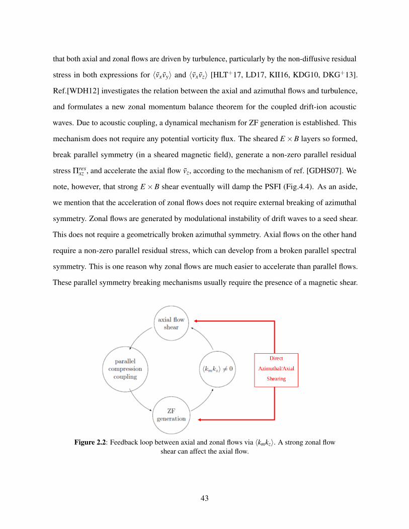
that both axial and zonal flows are driven by turbulence, particularly by the non-diffusive residual
stress in both expressions for 〈vxvy〉 and 〈vxvz〉 [HLT+17, LD17, KII16, KDG10, DKG+13].
Ref.[WDH12] investigates the relation between the axial and azimuthal flows and turbulence,
and formulates a new zonal momentum balance theorem for the coupled drift-ion acoustic
waves. Due to acoustic coupling, a dynamical mechanism for ZF generation is established. This
mechanism does not require any potential vorticity flux. The sheared E×B layers so formed,
break parallel symmetry (in a sheared magnetic field), generate a non-zero parallel residual
stress Πresxz , and accelerate the axial flow vz, according to the mechanism of ref. [GDHS07]. We
note, however, that strong E×B shear eventually will damp the PSFI (Fig.4.4). As an aside,
we mention that the acceleration of zonal flows does not require external breaking of azimuthal
symmetry. Zonal flows are generated by modulational instability of drift waves to a seed shear.
This does not require a geometrically broken azimuthal symmetry. Axial flows on the other hand
require a non-zero parallel residual stress, which can develop from a broken parallel spectral
symmetry. This is one reason why zonal flows are much easier to accelerate than parallel flows.
These parallel symmetry breaking mechanisms usually require the presence of a magnetic shear.
Figure 2.2: Feedback loop between axial and zonal flows via 〈kmkz〉. A strong zonal flowshear can affect the axial flow.
43
However, such mechanisms are not relevant to CSDX, since B is constant and magnetic shear
is absent. Symmetry breaking is then provided by a dynamical mechanism, based on DWs and
momentum evolution [LDXT16]. The growth rate of the DWs in CSDX is determined by the
frequency shift: |γ| ∼ ω?−ω. A test flow shear v′z changes this frequency shift, setting modes
with kmkz|v′z|> 0 to grow faster than those with kmkz|v′z|< 0, and causing a spectral imbalance in
the km− kz space to develop. This creates a parallel residual stress Πresxz =−|χres
z |∇vz. The latter
reinforces the test shear, and amplifies the parallel flow through a process of ’negative viscosity’.
If v′z keeps increasing, the parallel shear flow instability (PSFI) will occur [KIIe5, KIK+16].
When the PSFI is turned on, ∇vz saturates at the PSFI linear threshold and the total viscosity
remains positive: χtotz = χDW
z +χPSFIz −|χres
z | > 0. In CSDX, no external axial momentum is
injected into the plasma, and ∇vz never exceeds the critical value necessary to destabilize the
PSFI [LD17]. Turbulence production thus primarily accelerates the axial flow in CSDX without
destabilizing it.
2.4.1 Calculating the Expression for 〈vxvz〉
In the near adiabatic limit, the expression for the parallel stress 〈vxvz〉 is obtained by
writing vx =−ikmρscsφ and using eq.(2.1c) to get:
〈vxvz〉=−|γm|〈δv2
x〉|ω|2
dvz
dx+ 〈kmkz〉ρsc3
s
[ |γm||ω|2
+(ω?−ωr)
|ω|α
](2.25)
In obtaining the expression for 〈vxvz〉, we neglected the contribution of the flow shear V ′0
with respect to the wave frequency ω, as we did in the expression for 〈vxvy〉. Just like χy, the
total parallel diffusivity χz is equal to the sum of the resonant and the non-resonant part. The
first component of eq.(2.25) is a diffusive term that is written as −χzdvz/dx, where the turbulent
diffusivity is:
χz =|γm|〈δv2
x〉|ω|2
= τc〈δv2x〉= lmix
√f ε (2.26)
44
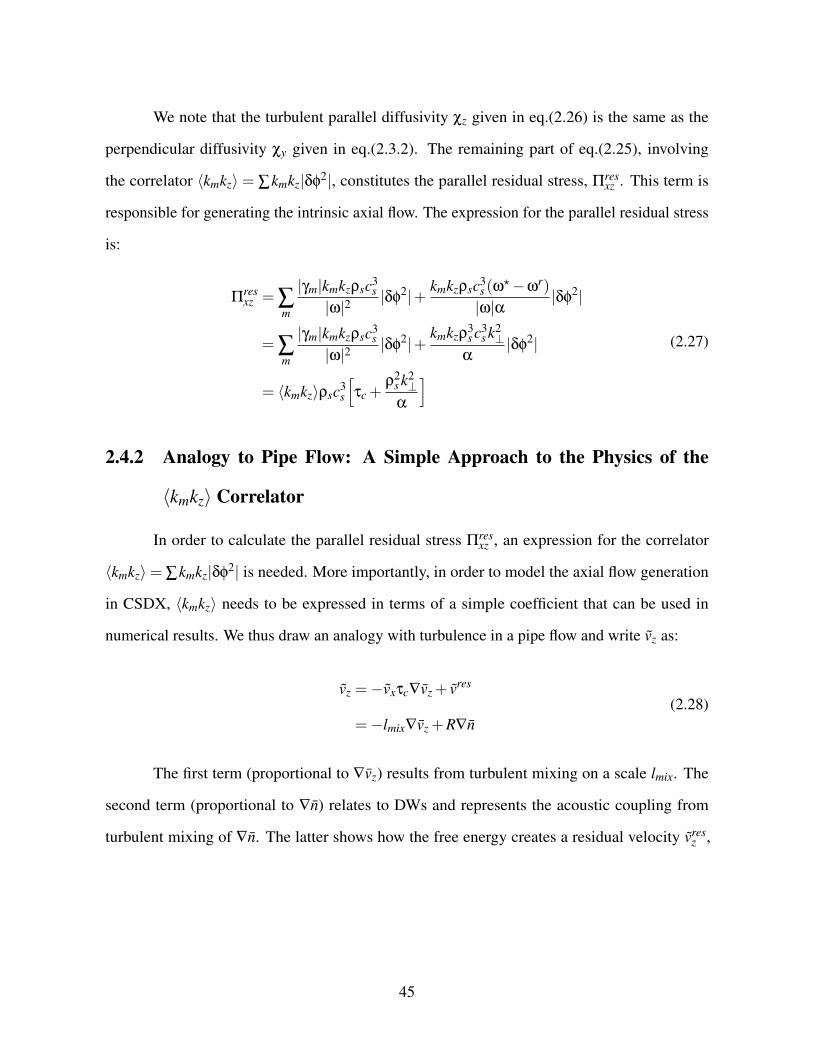
We note that the turbulent parallel diffusivity χz given in eq.(2.26) is the same as the
perpendicular diffusivity χy given in eq.(2.3.2). The remaining part of eq.(2.25), involving
the correlator 〈kmkz〉 = ∑kmkz|δφ2|, constitutes the parallel residual stress, Πresxz . This term is
responsible for generating the intrinsic axial flow. The expression for the parallel residual stress
is:
Πresxz = ∑
m
|γm|kmkzρsc3s
|ω|2|δφ
2|+ kmkzρsc3s (ω
?−ωr)
|ω|α|δφ
2|
= ∑m
|γm|kmkzρsc3s
|ω|2|δφ
2|+kmkzρ
3s c3
s k2⊥
α|δφ
2|
= 〈kmkz〉ρsc3s
[τc +
ρ2s k2⊥
α
](2.27)
2.4.2 Analogy to Pipe Flow: A Simple Approach to the Physics of the
〈kmkz〉 Correlator
In order to calculate the parallel residual stress Πresxz , an expression for the correlator
〈kmkz〉= ∑kmkz|δφ2| is needed. More importantly, in order to model the axial flow generation
in CSDX, 〈kmkz〉 needs to be expressed in terms of a simple coefficient that can be used in
numerical results. We thus draw an analogy with turbulence in a pipe flow and write vz as:
vz =−vxτc∇vz + vres
=−lmix∇vz +R∇n(2.28)
The first term (proportional to ∇vz) results from turbulent mixing on a scale lmix. The
second term (proportional to ∇n) relates to DWs and represents the acoustic coupling from
turbulent mixing of ∇n. The latter shows how the free energy creates a residual velocity vresz ,
45
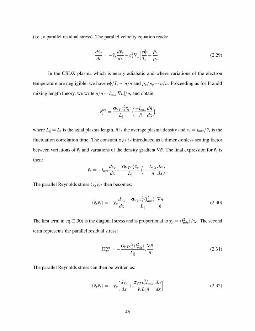
(i.e., a parallel residual stress). The parallel velocity equation reads:
dvz
dt=−vx
dvz
dx− c2
s ∇z
[eφ
Te+
pe
pe
](2.29)
In the CSDX plasma which is nearly adiabatic and where variations of the electron
temperature are negligible, we have eφ/Te ∼ n/n and pe/pe ∼ n/n. Proceeding as for Prandtl
mixing length theory, we write n/n∼ lmix|∇n|/n, and obtain:
vresz =
σV T c2s τc
L‖.(−lmix
ndndx
)
where L‖ = Lz is the axial plasma length, n is the average plasma density and τc = lmix/vx is the
fluctuation correlation time. The constant σV T is introduced as a dimensionless scaling factor
between variations of vz and variations of the density gradient ∇n. The final expression for vz is
then:
vz =−lmixdvz
dx+
σV T c2s τc
L‖.(− lmix
ndndx
),
The parallel Reynolds stress 〈vxvz〉 then becomes:
〈vxvz〉=−χzdvz
dx− σV T c2
s 〈l2mix〉
L‖.∇nn
(2.30)
The first term in eq.(2.30) is the diagonal stress and is proportional to χz = 〈l2mix〉/τc. The second
term represents the parallel residual stress:
Πresxz =−σV T c2
s 〈l2mix〉
L‖.∇nn
(2.31)
The parallel Reynolds stress can then be written as:
〈vxvz〉=−χz
[dvz
dx+
σV T c2s lmix
vxL‖n.dndx
](2.32)
46
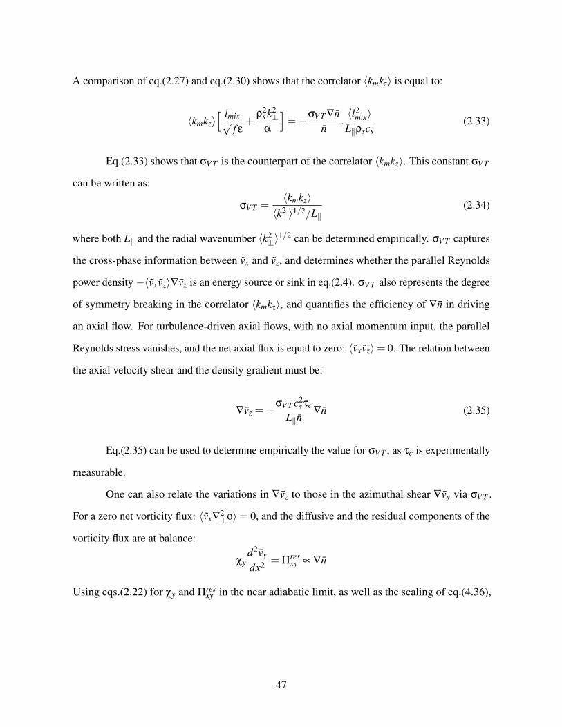
A comparison of eq.(2.27) and eq.(2.30) shows that the correlator 〈kmkz〉 is equal to:
〈kmkz〉[ lmix√
f ε+
ρ2s k2⊥
α
]=−σV T ∇n
n.〈l2
mix〉L‖ρscs
(2.33)
Eq.(2.33) shows that σV T is the counterpart of the correlator 〈kmkz〉. This constant σV T
can be written as:
σV T =〈kmkz〉〈k2⊥〉1/2/L‖
(2.34)
where both L‖ and the radial wavenumber 〈k2⊥〉
1/2 can be determined empirically. σV T captures
the cross-phase information between vx and vz, and determines whether the parallel Reynolds
power density −〈vxvz〉∇vz is an energy source or sink in eq.(2.4). σV T also represents the degree
of symmetry breaking in the correlator 〈kmkz〉, and quantifies the efficiency of ∇n in driving
an axial flow. For turbulence-driven axial flows, with no axial momentum input, the parallel
Reynolds stress vanishes, and the net axial flux is equal to zero: 〈vxvz〉= 0. The relation between
the axial velocity shear and the density gradient must be:
∇vz =−σV T c2
s τc
L‖n∇n (2.35)
Eq.(2.35) can be used to determine empirically the value for σV T , as τc is experimentally
measurable.
One can also relate the variations in ∇vz to those in the azimuthal shear ∇vy via σV T .
For a zero net vorticity flux: 〈vx∇2⊥φ〉= 0, and the diffusive and the residual components of the
vorticity flux are at balance:
χyd2vy
dx2 = Πresxy ∝ ∇n
Using eqs.(2.22) for χy and Πresxy in the near adiabatic limit, as well as the scaling of eq.(4.36),
47
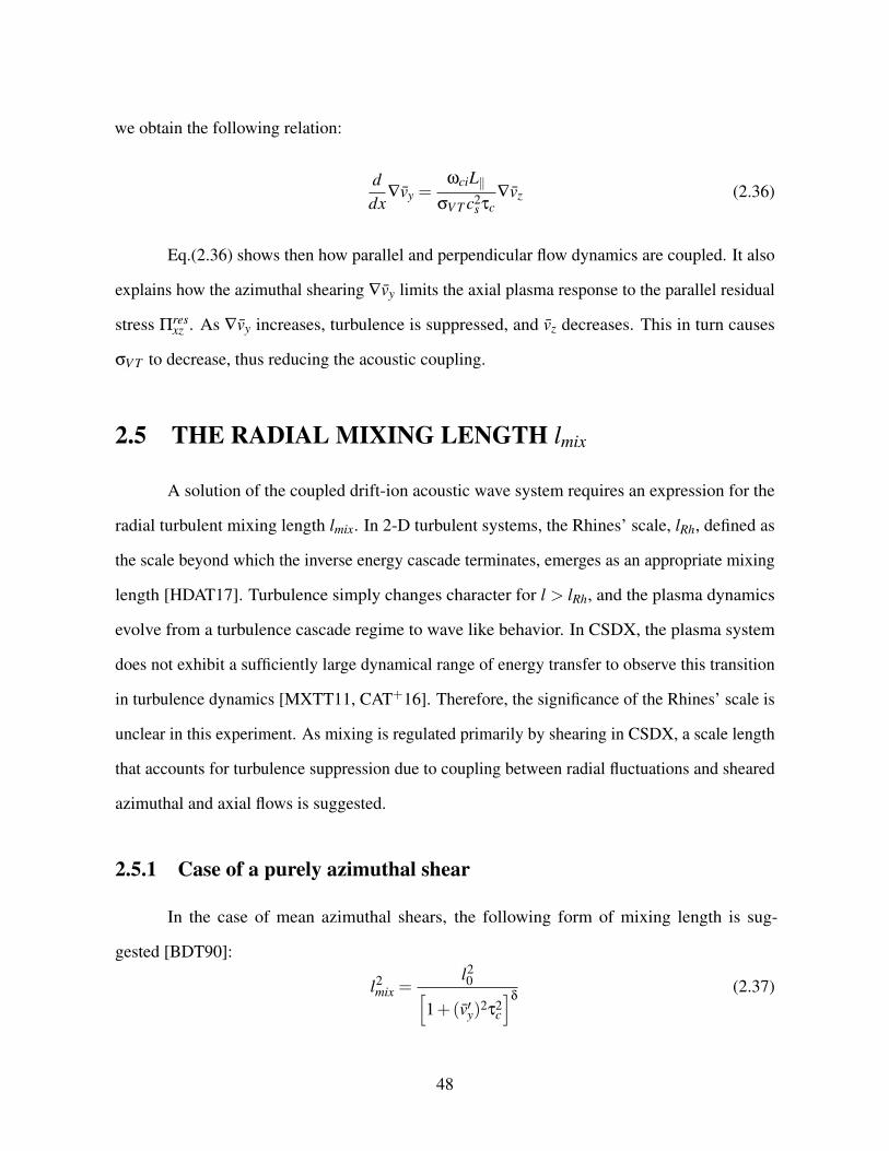
we obtain the following relation:
ddx
∇vy =ωciL‖
σV T c2s τc
∇vz (2.36)
Eq.(2.36) shows then how parallel and perpendicular flow dynamics are coupled. It also
explains how the azimuthal shearing ∇vy limits the axial plasma response to the parallel residual
stress Πresxz . As ∇vy increases, turbulence is suppressed, and vz decreases. This in turn causes
σV T to decrease, thus reducing the acoustic coupling.
2.5 THE RADIAL MIXING LENGTH lmix
A solution of the coupled drift-ion acoustic wave system requires an expression for the
radial turbulent mixing length lmix. In 2-D turbulent systems, the Rhines’ scale, lRh, defined as
the scale beyond which the inverse energy cascade terminates, emerges as an appropriate mixing
length [HDAT17]. Turbulence simply changes character for l > lRh, and the plasma dynamics
evolve from a turbulence cascade regime to wave like behavior. In CSDX, the plasma system
does not exhibit a sufficiently large dynamical range of energy transfer to observe this transition
in turbulence dynamics [MXTT11, CAT+16]. Therefore, the significance of the Rhines’ scale is
unclear in this experiment. As mixing is regulated primarily by shearing in CSDX, a scale length
that accounts for turbulence suppression due to coupling between radial fluctuations and sheared
azimuthal and axial flows is suggested.
2.5.1 Case of a purely azimuthal shear
In the case of mean azimuthal shears, the following form of mixing length is sug-
gested [BDT90]:
l2mix =
l20[
1+(v′y)2τ2c
]δ(2.37)
48
Here δ is the suppression parameter, τc is the fluctuation correlation time, and l0 is the
mixing scale for turbulence in CSDX in the absence of shear flow. When the azimuthal shearing
rate is greater than the fluctuations growth rate: v′y > |γm|, turbulent eddies are decorrelated and
turbulence is suppressed. Coupling between the azimuthal shearing and the turbulent radial
scattering of fluctuations can quench turbulence and decrease lmix. An empirical relation for
the scale length of turbulence l0 = [(k2r )
1/2]−1 is found by expressing the inverse radial wave
number k−1r as a function of the density fluctuations n normalized by the average plasma density
n [HDAT17]:
l0 ' 2.3ρ0.6s L0.3
n (2.38)
This suggests that the CSDX turbulent plasma diffusion coefficient scales like:
DCSDX ' DBρ0.6? (2.39)
where DB is the Bohm diffusive coefficient, and ρ? is the ion gyroradius normalized by the
inverse density gradient scale length: ρ? = ρ/Ln. Eq.(2.39) suggests that the scalings of diffusion
in CSDX fall in between the Bohm and gyroBohm diffusion scalings. For τc, we write:
1/τc =(
k2m(v′y)
2χy
)1/3(2.40)
where the wavenumber is km ' 1/l0 and the turbulent diffusivity is χy = τc〈δv2x〉= τc f ε. The
correlation time is then:
τc =[(v′y)2 f ε
l20
]−1/4
and the mixing length becomes:
l2mix = l2
0
[1+|v′y|l0√
f ε
]−1(2.41)
49
The structure of eq.(2.41) shows an intuitively plausible inverse relation between the shear and
the mixing length.
2.5.2 Case of azimuthal and axial shear
When both axial and azimuthal shear are present in the system, and when the azimuthal
shear rate is greater than the radial correlation rate: v′y >√
f ε/l0, the expression for the mixing
length becomes:
l2mix =
l20[
1+(
kmv′y + kzv′z)2
τ2c
] (2.42)
Here the wavenumbers can be chosen as: km = 1/l0 and kz = 1/L‖. The expression for the
mixing length is:
l2mix = l2
0
[1+( v′y
l0+
v′zL‖
)2 l20
f ε
]−1(2.43)
The structure of eq.(2.43) is not significantly different from that of eq.(2.41). Both
expressions show that lmix is inversely proportional to v′y/v′z: as the shear grows, the mixing
length lmix shrinks. This in turn reduces the turbulent energy ε, and increases the mean energy
because of total energy conservation. In CSDX, the effective mean azimuthal shear v′y dominates
the mean axial shear v′z.
50
2.6 SUMMARY AND DISCUSSION OF THE MODEL
In summary, the model consists of the equations:
∂n∂t
=− ∂
∂x〈vxn〉+Dc
∂2n∂x2 +Sn (2.44a)
∂vz
∂t=− ∂
∂x〈vxvz〉+νc,‖
∂2vz
∂x2 +Svz (2.44b)
∂vy
∂t=− ∂
∂x〈vxvy〉+νc,⊥
∂2vy
∂x2 −νin(vy− vn)−νiivy +Svy (2.44c)
∂ε
∂t−∂x(lmixε
1/2∂xε) =−〈nvx〉
dndx−〈vxvz〉
dvz
dx−〈vxvy〉
dvy
dx− ε3/2
lmix+P (2.44d)
The expressions for the turbulent fluxes and the Reynolds power density are:
〈nvx〉=−f ε
α.
k2⊥ρ2
s
1+ k2⊥ρ2
s.
1n0
dndx
(2.45a)
−∂〈vxvy〉
∂x=−lmix
√f ε
d2vy
dx2 −lmix√
f εωci
Ln(2.45b)
−〈vxvy〉dvy
dx=−lmix
√f ε
(dvy
dx
)2− vy
lmix√
f εωci
Ln(2.45c)
〈vxvz〉=−lmix√
f εdvz
dx+ 〈kmkz〉ρsc3
s
[ lmix√f ε
+ρ2
s k2⊥
α
](2.45d)
=−lmix√
f εdvz
dx− σV T c2
s 〈l2mix〉
L‖Ln(2.45e)
Here lmix and f are given by eq.(2.43) and eq.(2.15) respectively. The model evolves the
fields n, vy, vz and ε in space and time (x, t) using a slowly varying envelope approximation. In
addition, the model self consistently relates the evolution of turbulence to that of the parallel and
perpendicular flow dynamics. The coupling terms associating the turbulent energy to variations
51
of the mean profiles n, vy and vz, are expressed in terms of a mixing length lmix, the expression for
which depends on both axial and azimuthal shear (eq.(2.43)). The particle flux is purely diffusive:
〈nvx〉 = −D∇n. Both parallel and perpendicular Reynolds stresses consist of a diffusive part
(−χz∇vz and −χy∇vy), as well as a residual component proportional to ∇n that generates an
axial and an azimuthal flow.
The generated axial flow is associated with the correlator 〈kmkz〉 6= 0 that measures
the acoustic coupling. A version of this model introduces the empirical constant σV T in the
expression for 〈kmkz〉 (eq.(2.31)). This experimentally measurable constant relates the variations
of the axial shear to those of the density gradient, via eq.(4.36). It also shows how free energy
released from the density gradient can accelerate vz, even in the case of no axial momentum
input. In addition, this constant accounts for the strength of the parallel to perpendicular flow
coupling as: σV T ∼ 〈vxvz〉 ∼ 〈kmkz〉. This coupling is stated in eq.(2.36), which relates v′z to v′y
since both shears are dependent on the density gradient ∇n. Finally, we note that this model
manifests the well known relation between turbulence and azimuthal flows via the Reynolds
stress 〈vxvy〉 and also manifests a similar relation between fluctuations and axial flows via the
parallel Reynolds stress 〈vxvz〉. Numerical solutions of this model will be published in a future
work.
2.7 REDUCING THE MODEL
When the eddy turnover time τc = lmix/vx is smaller than the confinement time τcon f =
[n−1D∇2n]−1, the model can then be reduced to a 3 field model by slaving the expression for
ε to the mean profiles, and solving the equations for n, vy and vz. Experimental results from
CSDX show that the energy transfer to the axial flow via the parallel Reynolds power density:∫−∂x〈vxvz〉vzdx, i.e., the power exerted by turbulence on the axial flow, is less than that exerted
on the azimuthal profile via:∫−∂x〈vxvy〉vydx, by a factor of five [HLT+17, HLH+17]. The axial
52
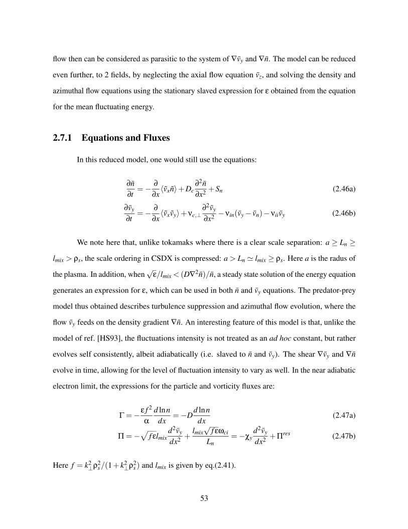
flow then can be considered as parasitic to the system of ∇vy and ∇n. The model can be reduced
even further, to 2 fields, by neglecting the axial flow equation vz, and solving the density and
azimuthal flow equations using the stationary slaved expression for ε obtained from the equation
for the mean fluctuating energy.
2.7.1 Equations and Fluxes
In this reduced model, one would still use the equations:
∂n∂t
=− ∂
∂x〈vxn〉+Dc
∂2n∂x2 +Sn (2.46a)
∂vy
∂t=− ∂
∂x〈vxvy〉+νc,⊥
∂2vy
∂x2 −νin(vy− vn)−νiivy (2.46b)
We note here that, unlike tokamaks where there is a clear scale separation: a ≥ Ln ≥
lmix > ρs, the scale ordering in CSDX is compressed: a > Ln ' lmix ≥ ρs. Here a is the radus of
the plasma. In addition, when√
ε/lmix < (D∇2n)/n, a steady state solution of the energy equation
generates an expression for ε, which can be used in both n and vy equations. The predator-prey
model thus obtained describes turbulence suppression and azimuthal flow evolution, where the
flow vy feeds on the density gradient ∇n. An interesting feature of this model is that, unlike the
model of ref. [HS93], the fluctuations intensity is not treated as an ad hoc constant, but rather
evolves self consistently, albeit adiabatically (i.e. slaved to n and vy). The shear ∇vy and ∇n
evolve in time, allowing for the level of fluctuation intensity to vary as well. In the near adiabatic
electron limit, the expressions for the particle and vorticity fluxes are:
Γ =−ε f 2
α
d lnndx
=−Dd lnn
dx(2.47a)
Π =−√
f εlmixd2vy
dx2 +lmix√
f εωci
Ln=−χy
d2vy
dx2 +Πres (2.47b)
Here f = k2⊥ρ2
s/(1+ k2⊥ρ2
s ) and lmix is given by eq.(2.41).
53
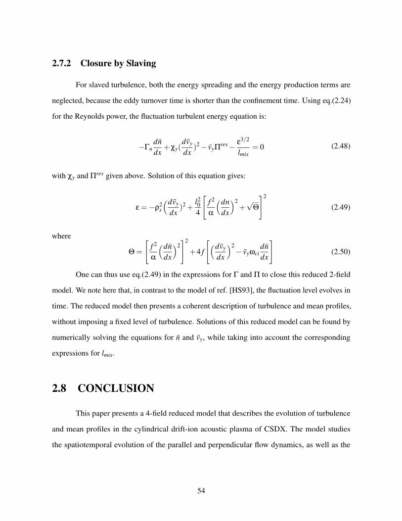
2.7.2 Closure by Slaving
For slaved turbulence, both the energy spreading and the energy production terms are
neglected, because the eddy turnover time is shorter than the confinement time. Using eq.(2.24)
for the Reynolds power, the fluctuation turbulent energy equation is:
−Γndndx
+χy(dvy
dx)2− vyΠ
res− ε3/2
lmix= 0 (2.48)
with χy and Πres given above. Solution of this equation gives:
ε =−ρ2s
(dvy
dx)2 +
l204
[f 2
α
(dndx
)2+√
Θ
]2
(2.49)
where
Θ =
[f 2
α
(dndx
)2]2
+4 f
[(dvy
dx
)2− vyωci
dndx
](2.50)
One can thus use eq.(2.49) in the expressions for Γ and Π to close this reduced 2-field
model. We note here that, in contrast to the model of ref. [HS93], the fluctuation level evolves in
time. The reduced model then presents a coherent description of turbulence and mean profiles,
without imposing a fixed level of turbulence. Solutions of this reduced model can be found by
numerically solving the equations for n and vy, while taking into account the corresponding
expressions for lmix.
2.8 CONCLUSION
This paper presents a 4-field reduced model that describes the evolution of turbulence
and mean profiles in the cylindrical drift-ion acoustic plasma of CSDX. The model studies
the spatiotemporal evolution of the parallel and perpendicular flow dynamics, as well as the
54
variations of the fluctuation intensity ε. Also, the model fills the gap in approach between a
0-D 2-field reduced model (n and vy), and a DNS of the three primitive equations. Moreover,
this reduced model yields a better physical interpretation for the mesoscopic results observed in
CSDX, while avoiding the computational cost of a full 4-field DNS.
A self-consistent description of the variations of three mean fields: density n, azimuthal
flow vy, and axial flow vz, in addition to the fluctuation intensity ε is presented here. Conservation
of the total (mean + turbulent) energy, including dissipation and internal energy production,
is a key element. Due to acoustic coupling, 〈n2 +(∇⊥φ)2 + v2z 〉 is the conserved energy field.
Because mixing occurs primarily by shearing in CSDX, the model employs a mixing length that
is inversely proportional to both axial and azimuthal flow shear (eq.(2.43)). However, we note
that in CSDX, v′y > v′z. The choice of a mixing length that is inversely proportional to the shear
closes the loop on the total energy, and allows development of improved confinement in CSDX.
Key elements of the model and its predications of experimental findings are:
1. Evolution of the profiles, including mean flows and turbulent stresses, in a cylindrical
plasma characterized by a constant magnetic field. The model explains how an increase
in the magnitude of B decreases the scale of turbulent transport and steepens the density
profile. Free energy released from ∇n accelerates then the azimuthal plasma flow vy, as
verified experimentally [CAT+16]. The current model is an extension of that presented in
ref.[HDAT17], where the predator/prey relation between DWs and ZFs was derived and
validated.
2. In the DW dominated plasma of CSDX, a test axial flow shear breaks the parallel symmetry,
which results in a residual stress Πresxz ∝ ∇n and an axial flow vz. Energy released from
∇n also accelerates vz via the parallel Reynolds stress 〈vxvz〉. This trend is in agreement
with the experimental results [HLT+17, HLH+17], and supports the analogy between the
plasma and an engine [KDG10]. The model thus unfolds a coupling relation between vz
and vy, as both flows are accelerated by the same free energy source.
55
3. The model reduces the evolution of plasma profiles to three fluxes: a particle diffusive flux,
as well as a parallel and perpendicular Reynolds stress with residual components Πresxz and
Πresxy . These fluxes regulate the transfer of energy between fluctuations and mean flows
and governs the ecology of flows and drift wave turbulence.
4. The model introduces an empirical constant σV T that measures the correlator 〈kmkz〉 =
∑m kmkz|φ|2. This correlator encodes the broken symmetry of turbulence, and quantifies the
efficiency of drift waves in driving Πresxz and vz through eq.(4.36). Because σV T measures
the cross phase relation between vx and vz, it determines the direction of energy transfer
between turbulence and axial flow.
5. Eq.(4.36) provides an expression for the critical density gradient necessary for onset of
an axial flow shear ∇vz. By balancing the residual and the diffusive components of the
parallel Reynolds stress, we obtain:
∣∣∣∇ncrit
n
∣∣∣= k2z v2
thνei
ω?L‖〈kmkz〉ρsc3
s τc
where τc is the correlation time. The model thus explains why a sheared vz flow was
observed only above a critical B value in CSDX, i.e., beyond a critical density gradient.
6. Through eq.(2.36), the model provides a direct expression for the parallel to perpendicular
flow coupling that is reported experimentally in refs.[HLT+17, HLH+17]. Because χy = χz,
and since both Πresxy and Πres
xz are proportional to ∇n, the relation:
d(∇vy)/dx∇vz
=Πres
xy
Πresxz
=ωciL‖
σV T c2s τc
is established, and σV T is interpreted as a measure of the magnitude of coupling between
∇vy and ∇vz.
56
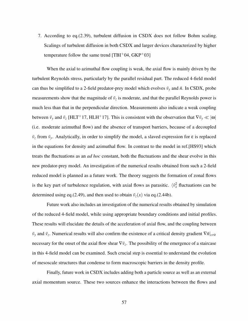
7. According to eq.(2.39), turbulent diffusion in CSDX does not follow Bohm scaling.
Scalings of turbulent diffusion in both CSDX and larger devices characterized by higher
temperature follow the same trend [TBI+04, GKP+03]
When the axial to azimuthal flow coupling is weak, the axial flow is mainly driven by the
turbulent Reynolds stress, particularly by the parallel residual part. The reduced 4-field model
can thus be simplified to a 2-field predator-prey model which evolves vy and n. In CSDX, probe
measurements show that the magnitude of vz is moderate, and that the parallel Reynolds power is
much less than that in the perpendicular direction. Measurements also indicate a weak coupling
between vy and vz [HLT+17, HLH+17]. This is consistent with the observation that ∇vy |ω|
(i.e. moderate azimuthal flow) and the absence of transport barriers, because of a decoupled
vz from vy. Analytically, in order to simplify the model, a slaved expression for ε is replaced
in the equations for density and azimuthal flow. In contrast to the model in ref.[HS93] which
treats the fluctuations as an ad hoc constant, both the fluctuations and the shear evolve in this
new predator-prey model. An investigation of the numerical results obtained from such a 2-field
reduced model is planned as a future work. The theory suggests the formation of zonal flows
is the key part of turbulence regulation, with axial flows as parasitic. 〈v2x fluctuations can be
determined using eq.(2.49), and then used to obtain vz(x) via eq.(2.44b).
Future work also includes an investigation of the numerical results obtained by simulation
of the reduced 4-field model, while using appropriate boundary conditions and initial profiles.
These results will elucidate the details of the acceleration of axial flow, and the coupling between
vy and vz. Numerical results will also confirm the existence of a critical density gradient ∇n|crit
necessary for the onset of the axial flow shear ∇vz. The possibility of the emergence of a staircase
in this 4-field model can be examined. Such crucial step is essential to understand the evolution
of mesoscale structures that condense to form macroscopic barriers in the density profile.
Finally, future work in CSDX includes adding both a particle source as well as an external
axial momentum source. These two sources enhance the interactions between the flows and
57
turbulence in the plasma, leading thereby to further coupling between vy and vz according to the
mechanism illustrated in fig.2.3. However, the azimuthal Reynolds power is much larger than
Drift Wave Turbulence
Zonal Flows Axial Flows
Coupling Relation
∇n Particle Source
Momentum Source
Figure 2.3: The future of CSDX: particle and axial momentum sources enhance theinteractions between flows and turbulence, and generate further coupling between the axial and
perpendicular flow dynamics.
the axial Reynolds power, so one may regard the axial flow evolution as parasitic to the drift
wavezonal flow system. This is consistent with the observation that V moderate azimuthal flow
shear) and thus there is no transport barrier.
58
2.9 Acknowledgments
The text and data in chapter 2 is a reprint of the material as it appears in ” The Ecology
of Flows and Drift Wave Turbulence in CSDX: a Model” in the Journal of Physics of Plasmas
25, 022301 (2018). Hajjar R. J., Diamond P.H., Tynan G.R., American Institute of Physics, 2018.
The dissertation author was the primary investigator and author of this article.
59
Chapter 3
MODELING ENHANCED
CONFINEMENT IN DRIFT WAVE
TURBULENCE
3.1 Introduction
Turbulent phenomena and their evolving properties in fluids are topics of both classical
and current significance. Of particular interest are the spectral features and transport properties
of turbulence in magnetized plasmas. Density and temperature gradients, typically present near
the edges of large scale magnetically confined devices, generate fluctuations that give rise to fully
developed drift wave (DW) instabilities. Such instabilities carry fluxes via cross-field transport
and limit the energy confinement time τE [Hor99, Gar01]. Suppression of these instabilities and
reduction of the cross-field transport rates are therefore essential requirements for achieving
enhanced confinement, in ITER and future tokamaks.
One way the plasma itself mitigates cross-field transport rates is via fluctuation driven
zonal flows (ZF). In laboratory plasmas, zonal flows are strongly sheared E×B layers. Generated
60
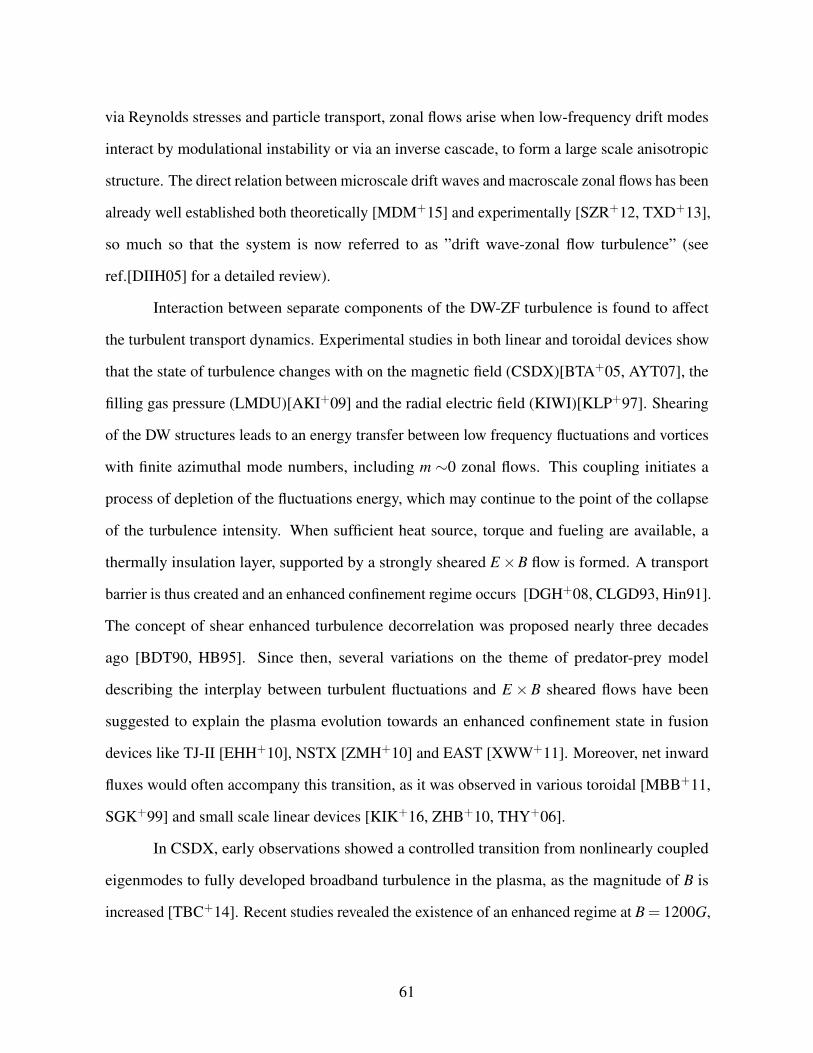
via Reynolds stresses and particle transport, zonal flows arise when low-frequency drift modes
interact by modulational instability or via an inverse cascade, to form a large scale anisotropic
structure. The direct relation between microscale drift waves and macroscale zonal flows has been
already well established both theoretically [MDM+15] and experimentally [SZR+12, TXD+13],
so much so that the system is now referred to as ”drift wave-zonal flow turbulence” (see
ref.[DIIH05] for a detailed review).
Interaction between separate components of the DW-ZF turbulence is found to affect
the turbulent transport dynamics. Experimental studies in both linear and toroidal devices show
that the state of turbulence changes with on the magnetic field (CSDX)[BTA+05, AYT07], the
filling gas pressure (LMDU)[AKI+09] and the radial electric field (KIWI)[KLP+97]. Shearing
of the DW structures leads to an energy transfer between low frequency fluctuations and vortices
with finite azimuthal mode numbers, including m ∼0 zonal flows. This coupling initiates a
process of depletion of the fluctuations energy, which may continue to the point of the collapse
of the turbulence intensity. When sufficient heat source, torque and fueling are available, a
thermally insulation layer, supported by a strongly sheared E×B flow is formed. A transport
barrier is thus created and an enhanced confinement regime occurs [DGH+08, CLGD93, Hin91].
The concept of shear enhanced turbulence decorrelation was proposed nearly three decades
ago [BDT90, HB95]. Since then, several variations on the theme of predator-prey model
describing the interplay between turbulent fluctuations and E ×B sheared flows have been
suggested to explain the plasma evolution towards an enhanced confinement state in fusion
devices like TJ-II [EHH+10], NSTX [ZMH+10] and EAST [XWW+11]. Moreover, net inward
fluxes would often accompany this transition, as it was observed in various toroidal [MBB+11,
SGK+99] and small scale linear devices [KIK+16, ZHB+10, THY+06].
In CSDX, early observations showed a controlled transition from nonlinearly coupled
eigenmodes to fully developed broadband turbulence in the plasma, as the magnitude of B is
increased [TBC+14]. Recent studies revealed the existence of an enhanced regime at B = 1200G,
61
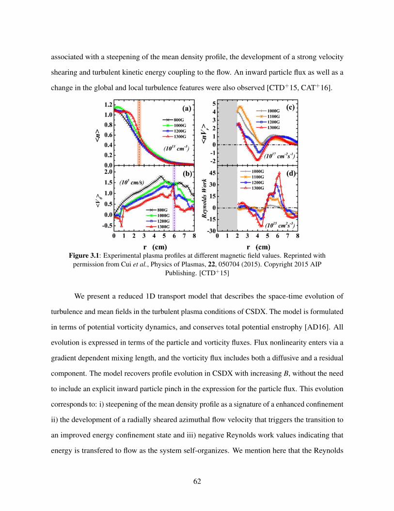
associated with a steepening of the mean density profile, the development of a strong velocity
shearing and turbulent kinetic energy coupling to the flow. An inward particle flux as well as a
change in the global and local turbulence features were also observed [CTD+15, CAT+16].
Figure 3.1: Experimental plasma profiles at different magnetic field values. Reprinted withpermission from Cui et al., Physics of Plasmas, 22, 050704 (2015). Copyright 2015 AIP
Publishing. [CTD+15]
We present a reduced 1D transport model that describes the space-time evolution of
turbulence and mean fields in the turbulent plasma conditions of CSDX. The model is formulated
in terms of potential vorticity dynamics, and conserves total potential enstrophy [AD16]. All
evolution is expressed in terms of the particle and vorticity fluxes. Flux nonlinearity enters via a
gradient dependent mixing length, and the vorticity flux includes both a diffusive and a residual
component. The model recovers profile evolution in CSDX with increasing B, without the need
to include an explicit inward particle pinch in the expression for the particle flux. This evolution
corresponds to: i) steepening of the mean density profile as a signature of a enhanced confinement
ii) the development of a radially sheared azimuthal flow velocity that triggers the transition to
an improved energy confinement state and iii) negative Reynolds work values indicating that
energy is transfered to flow as the system self-organizes. We mention here that the Reynolds
62
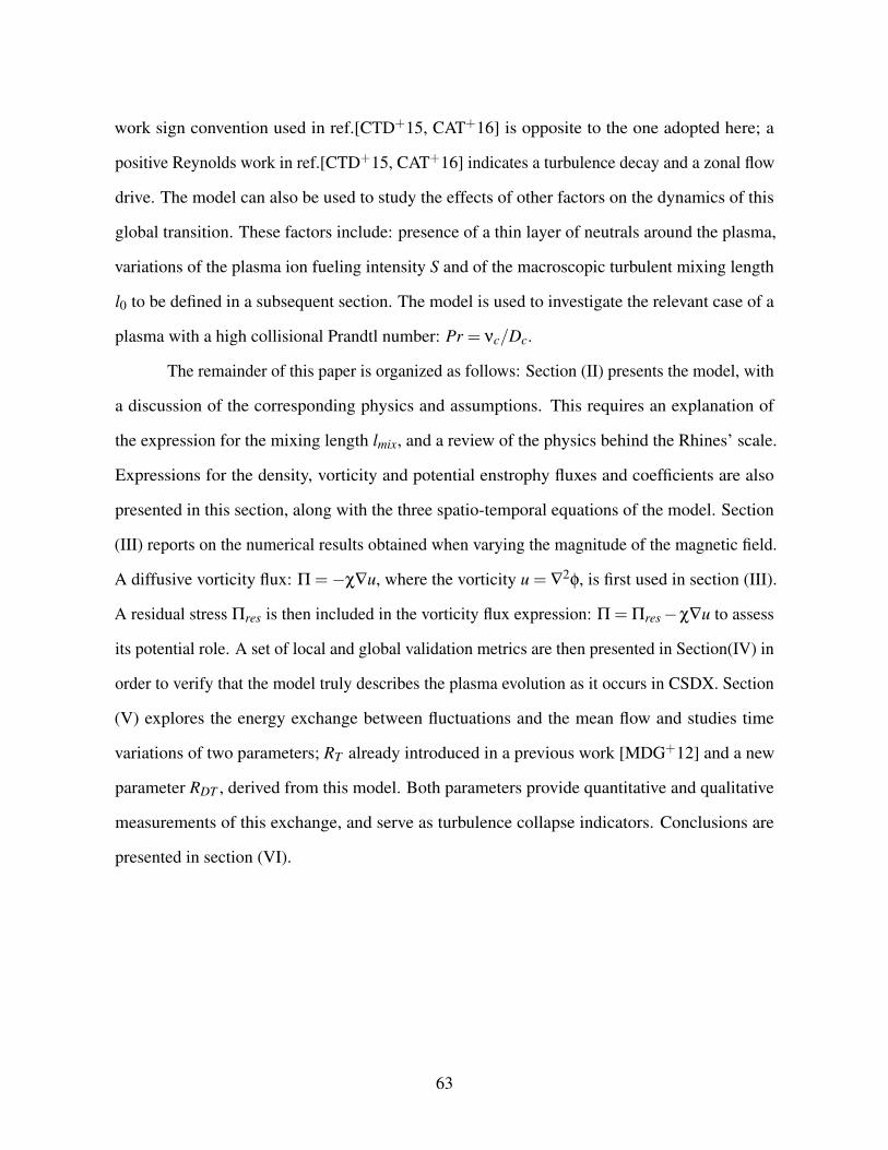
work sign convention used in ref.[CTD+15, CAT+16] is opposite to the one adopted here; a
positive Reynolds work in ref.[CTD+15, CAT+16] indicates a turbulence decay and a zonal flow
drive. The model can also be used to study the effects of other factors on the dynamics of this
global transition. These factors include: presence of a thin layer of neutrals around the plasma,
variations of the plasma ion fueling intensity S and of the macroscopic turbulent mixing length
l0 to be defined in a subsequent section. The model is used to investigate the relevant case of a
plasma with a high collisional Prandtl number: Pr = νc/Dc.
The remainder of this paper is organized as follows: Section (II) presents the model, with
a discussion of the corresponding physics and assumptions. This requires an explanation of
the expression for the mixing length lmix, and a review of the physics behind the Rhines’ scale.
Expressions for the density, vorticity and potential enstrophy fluxes and coefficients are also
presented in this section, along with the three spatio-temporal equations of the model. Section
(III) reports on the numerical results obtained when varying the magnitude of the magnetic field.
A diffusive vorticity flux: Π =−χ∇u, where the vorticity u = ∇2φ, is first used in section (III).
A residual stress Πres is then included in the vorticity flux expression: Π = Πres−χ∇u to assess
its potential role. A set of local and global validation metrics are then presented in Section(IV) in
order to verify that the model truly describes the plasma evolution as it occurs in CSDX. Section
(V) explores the energy exchange between fluctuations and the mean flow and studies time
variations of two parameters; RT already introduced in a previous work [MDG+12] and a new
parameter RDT , derived from this model. Both parameters provide quantitative and qualitative
measurements of this exchange, and serve as turbulence collapse indicators. Conclusions are
presented in section (VI).
63
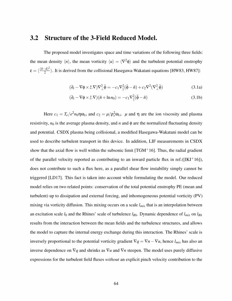
3.2 Structure of the 3-Field Reduced Model.
The proposed model investigates space and time variations of the following three fields:
the mean density 〈n〉, the mean vorticity 〈u〉 = 〈∇2φ〉 and the turbulent potential enstrophy
ε = 〈 (n−u)2
2 〉. It is derived from the collisional Hasegawa-Wakatani equations [HW83, HW87]:
(∂t−∇φ× z.∇)∇2⊥φ =−c1∇
2‖(φ− n)+ c2∇
2(∇2⊥φ) (3.1a)
(∂t−∇φ× z.∇)(n+ lnn0) =−c1∇2‖(φ− n) (3.1b)
Here c1 = Te/e2n0ηωci and c2 = µ/ρ2s ωci. µ and η are the ion viscosity and plasma
resistivity, n0 is the average plasma density, and n and φ are the normalized fluctuating density
and potential. CSDX plasma being collisional, a modified Hasegawa-Wakatani model can be
used to describe turbulent transport in this device. In addition, LIF measurements in CSDX
show that the axial flow is well within the subsonic limit [TGM+16]. Thus, the radial gradient
of the parallel velocity reported as contributing to an inward particle flux in ref.([IKI+16]),
does not contribute to such a flux here, as a parallel shear flow instability simply cannot be
triggered [LD17]. This fact is taken into account while formulating the model. Our reduced
model relies on two related points: conservation of the total potential enstrophy PE (mean and
turbulent) up to dissipation and external forcing, and inhomogeneous potential vorticity (PV)
mixing via vorticity diffusion. This mixing occurs on a scale lmix that is an interpolation between
an excitation scale l0 and the Rhines’ scale of turbulence lRh. Dynamic dependence of lmix on lRh
results from the interaction between the mean fields and the turbulence structures, and allows
the model to capture the internal energy exchange during this interaction. The Rhines’ scale is
inversely proportional to the potential vorticity gradient ∇q = ∇n−∇u, hence lmix has also an
inverse dependence on ∇q and shrinks as ∇u and ∇n steepen. The model uses purely diffusive
expressions for the turbulent field fluxes without an explicit pinch velocity contribution to the
64
particle flux. In fact, local expressions for the fluxes of n, u and ε as derived using the quasi-linear
theory are [ADG16]: Γn = −Dn∇n, Γε = −Dε∇ε and Π = Πres−χ∇u. A discussion of the
diffusion coefficients and the residual vorticity stress is deferred to a later section.
A full derivation of the model is available in ref.[AD16]. We mention here only the
relevant equations:
∂tu =−∂xΠ+µc∇2u (3.2a)
∂tn =−∂xΓn +Dc∇2n (3.2b)
∂tε =−∂xΓε +P− ε3/2− (Γn−Π)(∂xn−∂xu) (3.2c)
for mean density n and mean vorticity fields u, as well as for fluctuating potential enstrophy
ε = (n/n0−ρ2s ∇2eφ/Te)
2/2. Here, the fields are expanded into a mean and a fluctuating part:
n = 〈n〉+ n, vE = 〈v〉y+δv, u = 〈u〉+ u = ∂x〈v〉+ u. Fluxes of turbulent vorticity, density and
potential enstrophy fluxes are: Π = 〈vxu〉, Γn = 〈vxn〉 and Γε = 〈vxq2〉 respectively. Turbulent
enstrophy is related to the fluctuating potential vorticity q = n− u via: ε = 〈q2〉/2. µc and Dc are
plasma collisional viscosity and diffusivity, n and φ are normalized to n0 and Te/e, space and
times scales are normalized to ρs =√
miTe/eB and 1/ωci = mic/eB.
The first terms of the RHS of eqs.(3.2a-3.2c) represent a turbulent diffusive flux or
spreading of the corresponding field. In eq.(3.2c), P represents the enstrophy production due
to an external stirring, and replaces explicit linear instability which is not treated in this model.
Note that in this model formulation, the forcing serves only to initialize a background turbulence
level. It does not represent the turbulence drive in the steady state. Drive is due to ∇n relaxation,
i.e., Γn∇n term in eq.(3.2c). The turbulence and transport results are insensitive to the initializing
forcing, and we write it as: P =√
ε(u20− ε). This form of P reflects generation of enstrophy via
external stirring. Other forms of P ∝ ε are equally valid and generate similar results. Enstrophy
dissipation, proportional to ε3/2, is a direct outcome of the forward enstrophy cascade associated
65
with nonlinear dissipation of ε at smaller scales. The last term of eq.(3.2c) is a direct coupling
between the vorticity and density fluctuations, and is interpreted as an internal production of
potential enstrophy. As PV mixing occurs, mean PE values are converted into turbulent ones and
vice versa, while total PE is conserved. Eqs.(3.2a-3.2c) constitute a closed system that can be
solved numerically once expressions for the field fluxes are known. Since the model is diffusive,
expressions for the diffusion coefficients and the corresponding mixing length are thus needed.
Although CSDX is a cylindrical plasma, the previous equations are written in a 1D form. This
results from taking the axial and azimuthal average of the density, vorticity and enstrophy fields
in order to obtain the corresponding mean quantities: 〈n(r)〉, 〈u(r)〉= 〈∇2φ〉 and 〈ε(r)〉.
3.2.1 The Mixing Length
Central to the formulation of a Fickian flux is the use of a mixing length lmix. In this model
lmix is an interpolation between the external excitation dimension l0 and the Rhines’ scale of
turbulence lRh [Rhi75]. The dimension l0 is known from experiment, and thus an investigation of
lmix requires a study of the physics behind the Rhines’ scale. In 3D turbulence, vortex stretching
leads to enstrophy production that drives the fluid energy to smaller scales until it is removed
from the system by viscous dissipation. However, in quasi 2D turbulence, vortex stretching is by
definition inhibited and other nonlinear processes, such as vortex merging, play the prominent
role. In the 2D case, energy undergoes an inverse energy cascade towards larger scales, which
explains the emergence of large scale jets from small scale turbulent structures. As eddies
become bigger, their size increases and their overturning slows, which makes their dynamics
much more wave-like. The Rhines’ scale lRh can be interpreted as a transition length scale
between a turbulence dominated regime and wave-like dynamics [Rhi75], and is obtained by
balancing the turbulence characteristic rate, i.e., the eddy turnover rate, with the wave frequency.
In a DW system, an estimate of the eddy turnover rate is: 1/τc ≈ δv/lRh ≈√
ε, while the drift
wave frequency is: ω≈−kyvDe/(1+ k2⊥ρ2
s )≈ lRh∇q where vDe is the electron diamagnetic drift
66
velocity. Balancing these two scales then gives: lRh ≈√
ε/∇q =√
ε/∇(n−u).
In our model, l0 and lRh are the two significant length scales of the system. When
l0 lRh, the vorticity gradient is weak, and the natural estimate of the mixing length is simply
the external dimension: lmix ∼ l0. This prescription however is not accurate in the case of a
strong vorticity gradient, where ∇q can no longer be neglected. In this case, when the Rhines’
scale is much smaller than the stirring dimension (lRh l0), coupling between different scales is
stimulated. A reasonable estimate of the mixing length is then obtained by balancing the mean
kinetic energy dissipation rate and the mean PV gradient frequency [SM00]. The Rhines’ scale
is then the governing spatial structure for turbulence mixing in these cases of steep PV gradients,
generating lmix ∼ lRh. In between these two limiting cases, one should include the effect of finite
drift-Rossby frequency in lmix. This is achieved by writing lmix as an interpolation between l0
and lRh:
l2mix =
l20
1+(l0/lRh)2 =l20
1+ l20(∂x(n−u))2/ε
(3.3)
3.2.2 Expressions for the Turbulent Fluxes
Expressions for the turbulent density and vorticity fluxes were previously derived using
quasi-linear theory [ADG16]. In the near adiabatic regime in which parallel diffusion timescale
is the smallest characteristic time scale of the system, and in the absence of any shear, the drift
wave frequency is ω? = ωr = vdkm/(1+ k2⊥) where k2
⊥ =−∇2⊥φ/φ. Expressions for the fluxes
67
and the diffusion coefficients are:
Γn =−Dn∂x〈n〉 (3.4a)
Π = (χ−Dn)∂x〈n〉−χ∂2x〈v〉= Πres−χ∂x〈u〉 (3.4b)
Dn = ∑m
k2⊥
1+ k2⊥
k2mα〈δφ
2m〉 (3.4c)
χ = ∑m
|γm||V0−ω/km|2
〈δφ2m〉 (3.4d)
Here the dimensionless electron drift velocity is vd(x) =−d lnn0(x)/dx = χ∇n and the
plasma flow velocity is V0 = 〈v〉. The mode number is m = (m,n,l) with m, n and l being the az-
imuthal, axial and radial mode numbers respectively. ω = ωr + i|γm| is the mode eigenfrequency,
km and k‖ are the azimuthal and parallel wave numbers and α = ηk2‖ is the parallel diffusion rate.
The residual stress Πres in eq.(4.16) originates from a decomposition of the Reynolds
stress into a diffusive and non-diffusive components, and appears when the off-diagonal terms
of the poloidal Reynolds stress does not vanish. This results as a consequence of a symmetry
breaking mechanism in 〈krkθ〉 where 〈. . .〉 is a spectral average [DMG+09, GDH08]. Physically,
Πres converts parts of the diving particle flux to an azimuthal flow. Πres is responsible of
generation of plasma flows through the density gradient, even in the absence of any magnetic
shear [LDXT16]. Using quasi-linear theory, the residual stress Πres = Γn/n−χvd [ADG16].
In the adiabatic regime, the first term in the expression of Πres is negligible with respect to
the second one, simply because it is proportional to 1/α and α 1. One can thus label it as
the non-adiabatic term. When no flow is present, or when the flow velocity V0 is constant, the
vorticity flux reduces to Πres. Writing Γε =−Dε∂xε and plugging in the model equations, we
68
obtain the final form for the three field equations:
∂tn = ∂x[Dn∂xn]+Dc∂2xn (3.5a)
∂tu = ∂x[χ∂xu]+µc∂2xu−∂x[Πres] (3.5b)
∂tε = ∂x[Dε∂xε]+Πres(∂xn−∂xu)− (χ∂xu−Dn∂xn)(∂xn−∂xu)− ε3/2 +
√ε(u2
0− ε) (3.5c)
Eqs.(3.5a-3.5c) are rearranged and integrated to give:
∫ L
0∂t(ε+
(n−u)2
2)dx =
∫ L
0(P− ε
3/2−∂xΓε− (Γn−Π)(∂xn−∂xu)+(n−u)(∂tn−∂tu))dx
=∫ L
0(P− ε
3/2)dx
(3.6)
after neglecting the terms proportional to Dc and µc. This shows that the system conserves total
PE up to forcing and dissipation, as a result of enstrophy exchange between mean fields and
fluctuations. The internal turbulent PE production term is canceled by the corresponding loss
term in the evolution equation for the mean PE as a part of this enstrophy exchange. In view of
the total PE conservation elucidated above, we go back to eq.(3.3) to emphasize how crucial the
expression for lmix is in closing the feedback loop between the PV gradient and the corresponding
diffusion coefficient: as ∇q = ∇n−∇u steepens, the mean potential enstrophy (n−u)2
2 increases,
causing a drop in turbulent potential enstrophy ε as a result of total PE conservation. When ε
decreases, the mixing length and thus the corresponding PV diffusion coefficient shrink, leading
to a further increase in the PV gradient. Hence a closed feedback loop is generated.
69
3.2.3 Viscosity and Diffusion Coefficients
In the near adiabatic regime, the timescale ordering is: ηk2‖ωV ′0. Using |k2
m〈δφ2m〉|=
|〈δv2m〉| ≈ l2
mixε, the particle diffusion coefficient Dn is:
Dn = εl2mix/α (3.7)
where the resistive parallel diffusion rate has been rescaled as: α = (1+ k2⊥)α/k2
⊥. From dimen-
sional analysis, α is proportional to√
ε and the particle diffusion coefficient is: Dn = l2mix√
ε. As
for the vorticity diffusion coefficient, χ is not dominated by a large resistive parallel diffusion
rate. Unlike the expression for Dn, the denominator of eq.(3.4d) represents the competition
between the flow shear V ′0 and the wave frequency ω. In the absence of shear, instabilities are
density gradient driven collisional DWs, that are damped by viscous dissipation. Their growth
rate is then that of a drift wave: |γDW |= ω2/α, reduced by the dissipation rate |γµ|. The vorticity
diffusion coefficient is then:
χ = ∑m
(|γDW |− |γµ|)|k2m〈δφ2
m〉|ω2 = ∑
m
ω2
α|k2
m〈δφ2m〉|
ω2 ∼ εl2mixα
When a flow shear V ′0 is present, the vorticity diffusion coefficient χ is reduced, as the net
turbulence correlation time decreases. When incorporating the shear effect into the turbulence
correlation time, 1/α becomes: 1/α' 1/√
(k⊥δv)2 +(V ′0)2 ' 1/
√ε+q2, reflecting enstrophy
generation and presence of flow shear respectively. The vorticity diffusion coefficient χ then
becomes:
χ = εl2mix/
√ε+q2 = l2
mixε/√
α2 + cuu2 (3.8)
Here a coefficient cu reflecting the strength of the shear flow has been added to the
expression of χ. We will show later on that the numerical solutions for this model are insensitive
to the parameter cu. In a stationary regime,√
ε > q and the vorticity coefficient χ =√
εl2mix
70
found previously [BLSY98] is recovered. In a strong shear regime where q >√
ε, the vorticity
coefficient is χ = εl2mix/|q|. Finally, we use the following expression for Dε: Dε = l2
mixε/α. We
mention here that the model includes three different time scales: the wave frequency and growth
rate inverse time scales ω−1m and |γ|−1 appearing in the spectral sums of the diffusion coefficients
expressions, the correlation or eddy turnover time ε−1/2 appearing in the enstrophy equation,
and a diffusive time scale which characterizes the evolution of the mean field quantities as a
result of turbulent fluxes evolution. While the first two are fast time scales, the last one is a slow
(diffusive) one.
3.3 Model Predictions of Plasma Profiles.
In order to compare the model predictions to the experimental results obtained from
CSDX, we present in this section the density and vorticity profiles numerically predicted by the
model for different B values. Two forms of vorticity fluxes are considered. First, a diffusive
vorticity form: Π =−∂xu. Then, a residual stress Πres is added to the vorticity flux. The two
cases are then compared to evaluate any potential role of Πres. Before proceeding, we lay out the
experimental parameters of CSDX cylindrical magnetized helicon plasma: the plasma column has
a total length L = 2.8m and a radius a = 10cm. Argon plasma with the following characteristics
is produced: ne = 1013cm−3, Te = 4eV and Ti = 0.3−0.7eV . The magnitude of the magnetic
field B ranges between 800G and 1300G, giving ω−1ci ≈ 30µs and ρs = Cs/ωci ≈ 1cm where
Cs =√
Te/mi is the plasma sound speed. Argon neutrals are radially injected at a constant
flow rate of 25 sccm, and the corresponding neutral gas pressure Pgas = 3.2mTorr is equivalent
to a neutral density nn = 1014cm−3 [CTD+15, CAT+16]. Plasma neutral ionization rate at
Te = 5eV is S = nenn〈σionve〉 = 1017cm−3s−1, where 〈σionve〉 = 10−10cm3/s is the ionization
rate coefficient at 5eV. These values will be used in our calculations, in order to benchmark our
model predictions to the experimental results.
71
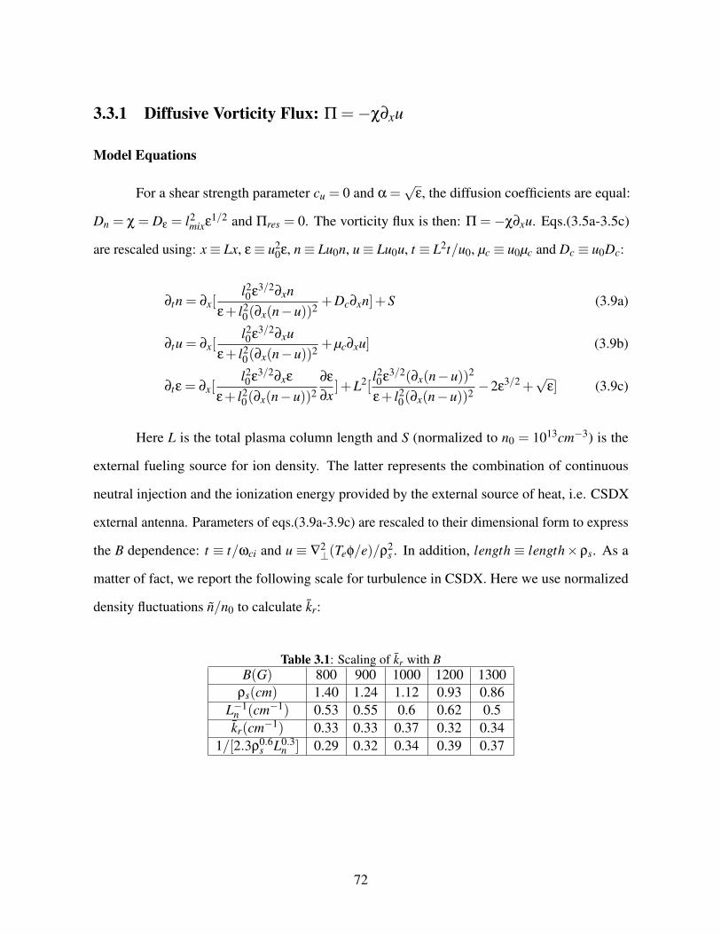
3.3.1 Diffusive Vorticity Flux: Π =−χ∂xu
Model Equations
For a shear strength parameter cu = 0 and α =√
ε, the diffusion coefficients are equal:
Dn = χ = Dε = l2mixε1/2 and Πres = 0. The vorticity flux is then: Π = −χ∂xu. Eqs.(3.5a-3.5c)
are rescaled using: x≡ Lx, ε≡ u20ε, n≡ Lu0n, u≡ Lu0u, t ≡ L2t/u0, µc ≡ u0µc and Dc ≡ u0Dc:
∂tn = ∂x[l20ε3/2∂xn
ε+ l20(∂x(n−u))2
+Dc∂xn]+S (3.9a)
∂tu = ∂x[l20ε3/2∂xu
ε+ l20(∂x(n−u))2
+µc∂xu] (3.9b)
∂tε = ∂x[l20ε3/2∂xε
ε+ l20(∂x(n−u))2
∂ε
∂x]+L2[
l20ε3/2(∂x(n−u))2
ε+ l20(∂x(n−u))2
−2ε3/2 +
√ε] (3.9c)
Here L is the total plasma column length and S (normalized to n0 = 1013cm−3) is the
external fueling source for ion density. The latter represents the combination of continuous
neutral injection and the ionization energy provided by the external source of heat, i.e. CSDX
external antenna. Parameters of eqs.(3.9a-3.9c) are rescaled to their dimensional form to express
the B dependence: t ≡ t/ωci and u ≡ ∇2⊥(Teφ/e)/ρ2
s . In addition, length ≡ length×ρs. As a
matter of fact, we report the following scale for turbulence in CSDX. Here we use normalized
density fluctuations n/n0 to calculate kr:
Table 3.1: Scaling of kr with BB(G) 800 900 1000 1200 1300
ρs(cm) 1.40 1.24 1.12 0.93 0.86L−1
n (cm−1) 0.53 0.55 0.6 0.62 0.5kr(cm−1) 0.33 0.33 0.37 0.32 0.34
1/[2.3ρ0.6s L0.3
n ] 0.29 0.32 0.34 0.39 0.37
72
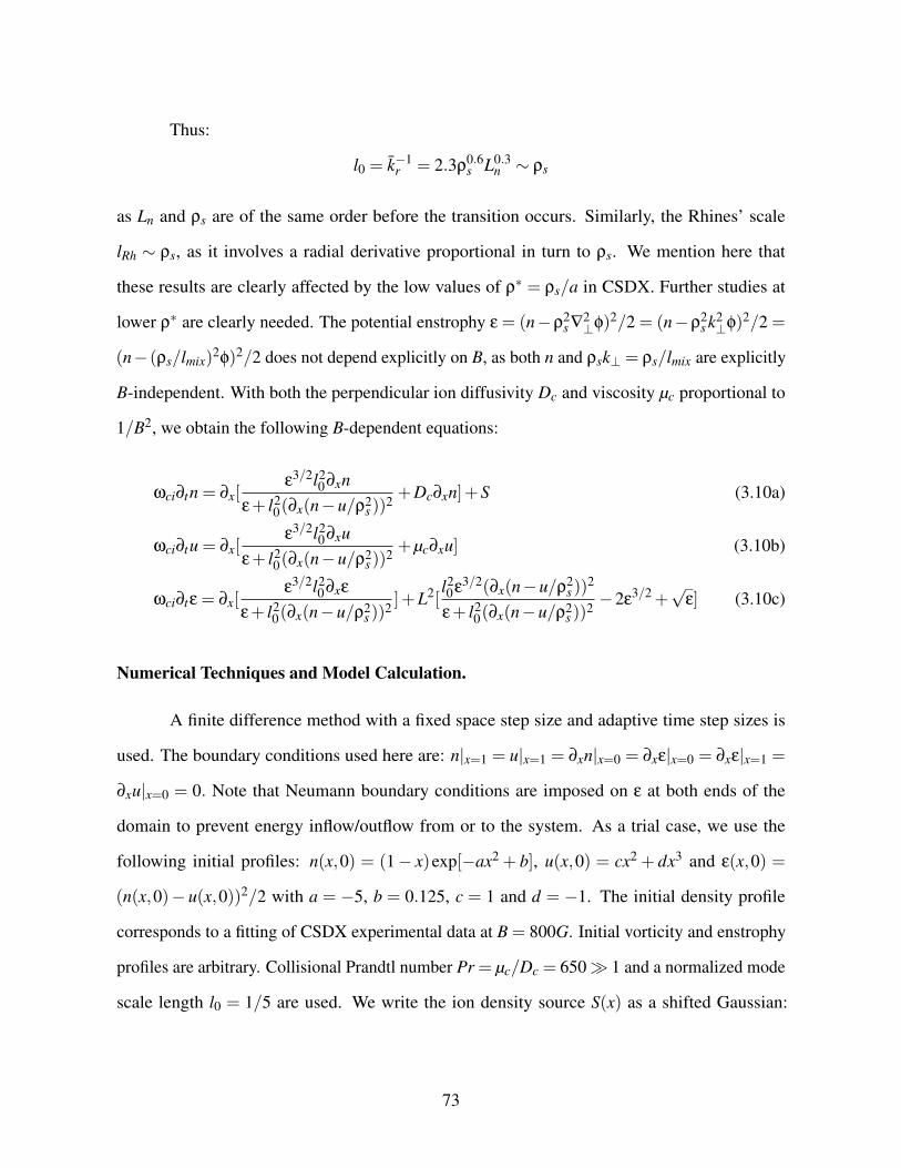
Thus:
l0 = k−1r = 2.3ρ
0.6s L0.3
n ∼ ρs
as Ln and ρs are of the same order before the transition occurs. Similarly, the Rhines’ scale
lRh ∼ ρs, as it involves a radial derivative proportional in turn to ρs. We mention here that
these results are clearly affected by the low values of ρ∗ = ρs/a in CSDX. Further studies at
lower ρ∗ are clearly needed. The potential enstrophy ε = (n−ρ2s ∇2⊥φ)2/2 = (n−ρ2
s k2⊥φ)2/2 =
(n− (ρs/lmix)2φ)2/2 does not depend explicitly on B, as both n and ρsk⊥ = ρs/lmix are explicitly
B-independent. With both the perpendicular ion diffusivity Dc and viscosity µc proportional to
1/B2, we obtain the following B-dependent equations:
ωci∂tn = ∂x[ε3/2l2
0∂xnε+ l2
0(∂x(n−u/ρ2s ))
2+Dc∂xn]+S (3.10a)
ωci∂tu = ∂x[ε3/2l2
0∂xuε+ l2
0(∂x(n−u/ρ2s ))
2+µc∂xu] (3.10b)
ωci∂tε = ∂x[ε3/2l2
0∂xε
ε+ l20(∂x(n−u/ρ2
s ))2]+L2[
l20ε3/2(∂x(n−u/ρ2
s ))2
ε+ l20(∂x(n−u/ρ2
s ))2−2ε
3/2 +√
ε] (3.10c)
Numerical Techniques and Model Calculation.
A finite difference method with a fixed space step size and adaptive time step sizes is
used. The boundary conditions used here are: n|x=1 = u|x=1 = ∂xn|x=0 = ∂xε|x=0 = ∂xε|x=1 =
∂xu|x=0 = 0. Note that Neumann boundary conditions are imposed on ε at both ends of the
domain to prevent energy inflow/outflow from or to the system. As a trial case, we use the
following initial profiles: n(x,0) = (1− x)exp[−ax2 + b], u(x,0) = cx2 + dx3 and ε(x,0) =
(n(x,0)− u(x,0))2/2 with a = −5, b = 0.125, c = 1 and d = −1. The initial density profile
corresponds to a fitting of CSDX experimental data at B = 800G. Initial vorticity and enstrophy
profiles are arbitrary. Collisional Prandtl number Pr = µc/Dc = 650 1 and a normalized mode
scale length l0 = 1/5 are used. We write the ion density source S(x) as a shifted Gaussian:
73
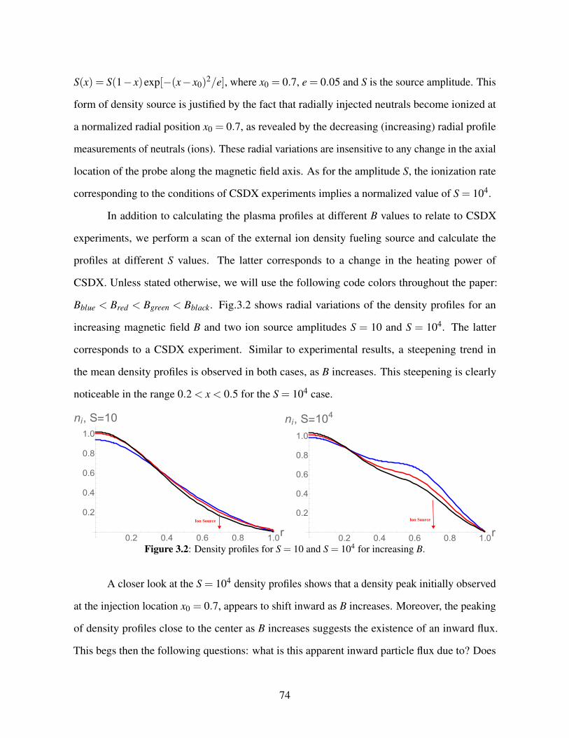
S(x) = S(1−x)exp[−(x−x0)2/e], where x0 = 0.7, e = 0.05 and S is the source amplitude. This
form of density source is justified by the fact that radially injected neutrals become ionized at
a normalized radial position x0 = 0.7, as revealed by the decreasing (increasing) radial profile
measurements of neutrals (ions). These radial variations are insensitive to any change in the axial
location of the probe along the magnetic field axis. As for the amplitude S, the ionization rate
corresponding to the conditions of CSDX experiments implies a normalized value of S = 104.
In addition to calculating the plasma profiles at different B values to relate to CSDX
experiments, we perform a scan of the external ion density fueling source and calculate the
profiles at different S values. The latter corresponds to a change in the heating power of
CSDX. Unless stated otherwise, we will use the following code colors throughout the paper:
Bblue < Bred < Bgreen < Bblack. Fig.3.2 shows radial variations of the density profiles for an
increasing magnetic field B and two ion source amplitudes S = 10 and S = 104. The latter
corresponds to a CSDX experiment. Similar to experimental results, a steepening trend in
the mean density profiles is observed in both cases, as B increases. This steepening is clearly
noticeable in the range 0.2 < x < 0.5 for the S = 104 case.
0.2 0.4 0.6 0.8 1.0r
0.2
0.4
0.6
0.8
1.0
ni, S=10
Ion Source
0.2 0.4 0.6 0.8 1.0r
0.2
0.4
0.6
0.8
1.0
ni, S=104
Ion Source
Figure 3.2: Density profiles for S = 10 and S = 104 for increasing B.
A closer look at the S = 104 density profiles shows that a density peak initially observed
at the injection location x0 = 0.7, appears to shift inward as B increases. Moreover, the peaking
of density profiles close to the center as B increases suggests the existence of an inward flux.
This begs then the following questions: what is this apparent inward particle flux due to? Does
74
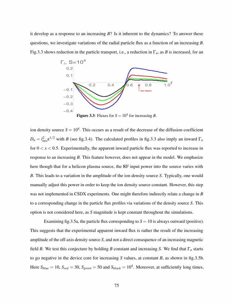
it develop as a response to an increasing B? Is it inherent to the dynamics? To answer these
questions, we investigate variations of the radial particle flux as a function of an increasing B.
Fig.3.3 shows reduction in the particle transport, i.e., a reduction in Γn, as B is increased, for an
0.2 0.4 0.6 0.8 1.0r
-0.4
-0.3
-0.2
-0.1
0.1
0.2
Γi, S=104
Ion Source
Figure 3.3: Fluxes for S = 104 for increasing B.
ion density source S = 104. This occurs as a result of the decrease of the diffusion coefficient
Dn = l2mixε1/2 with B (see fig.3.4). The calculated profiles in fig.3.3 also imply an inward Γn
for 0 < x < 0.5. Experimentally, the apparent inward particle flux was reported to increase in
response to an increasing B. This feature however, does not appear in the model. We emphasize
here though that for a helicon plasma source, the RF input power into the source varies with
B. This leads to a variation in the amplitude of the ion density source S. Typically, one would
manually adjust this power in order to keep the ion density source constant. However, this step
was not implemented in CSDX experiments. One might therefore indirectly relate a change in B
to a corresponding change in the particle flux profiles via variations of the density source S. This
option is not considered here, as S magnitude is kept constant throughout the simulations.
Examining fig.3.5a, the particle flux corresponding to S = 10 is always outward (positive).
This suggests that the experimental apparent inward flux is rather the result of the increasing
amplitude of the off-axis density source S, and not a direct consequence of an increasing magnetic
field B. We test this conjecture by holding B constant and increasing S. We find that Γn starts
to go negative in the device core for increasing S values, at constant B, as shown in fig.3.5b.
Here Sblue = 10, Sred = 30, Sgreen = 50 and Sblack = 104. Moreover, at sufficiently long times,
75
0.2 0.4 0.6 0.8 1.0r0.005
0.010
0.015
0.020
0.025
0.030
Diffusion coefficient, Dn
Figure 3.4: Diffusion coefficient for increasing B.
0.2 0.4 0.6 0.8 1.0r
0.005
0.010
0.015
0.020
0.025
0.030
Γi, S=10
Ion Source
0.2 0.4 0.6 0.8 1.0r
-0.04
-0.03
-0.02
-0.01
0.01
0.02
Γi at fixed B
Ion Source
Figure 3.5: Particle flux at S = 10 for increasing B and particle flux at constant B andincreasing S : Sblue < Sred < Sgreen < Sblack.
the calculated particle flux saturates, and Γn profiles are positive and show no indication of
inward flux (fig.3.6). We conclude then that the experimentally reported apparent inward flux
appears to be a consequence of a change in the source amplitude and its position. Thus, we
recover the apparent inward flux semi-qualitatively, using a diffusive model for Γn =−∂xn (no
particle pinch Vpinch, i.e., no off-diagonal term in Γn). It is essential to note here that experiments
corresponding to different heating powers have been performed in CSDX. Data collected from
these experiments show a dependence of both the direction and the amplitude of the particle flux
Γn on the input heating power. Further investigation of this data is of crucial importance to fully
understand the nature of this apparent inward flux.
In order to determine if the model captures the DW-ZF interactions in CSDX, we examine
variations of the shear flow and of the Reynolds work with B. Fig.3.7a shows the existence
of an azimuthal velocity shear layer in the radial direction, that gradually becomes stronger
76
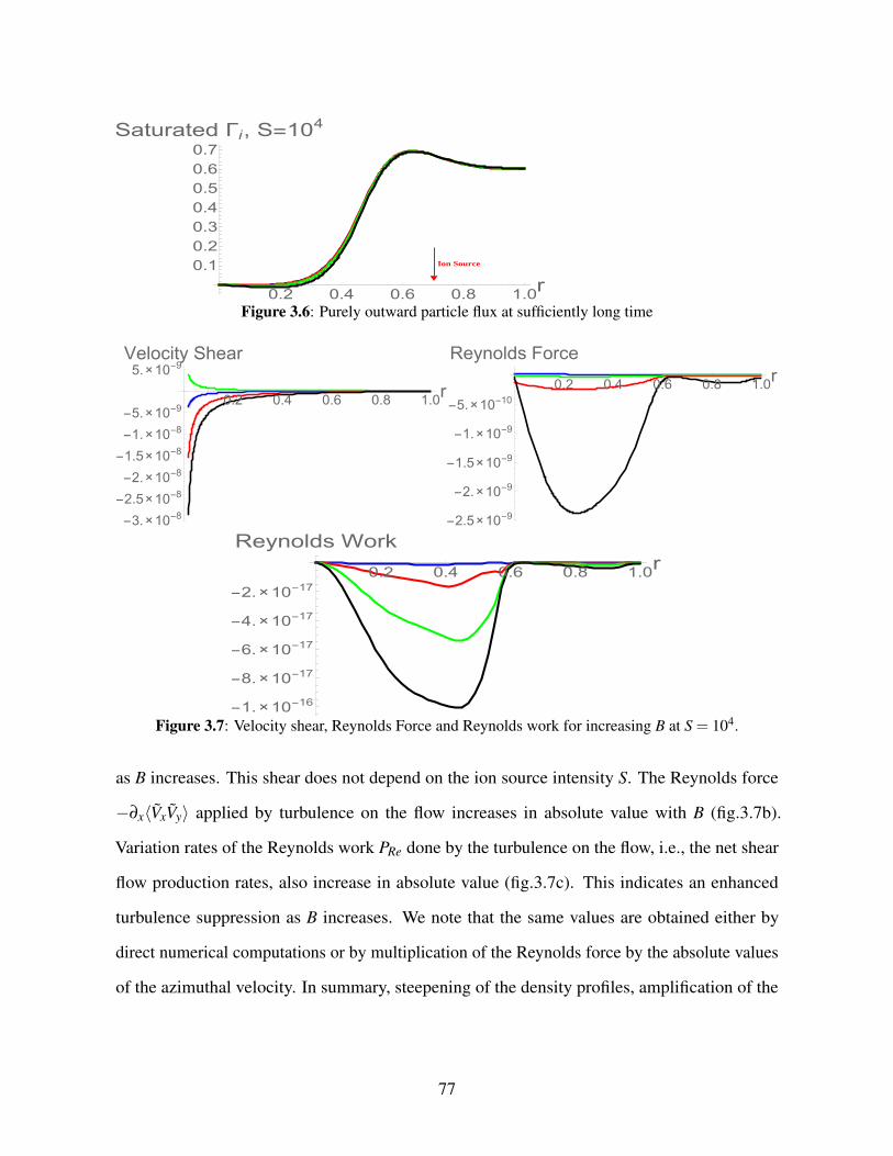
0.2 0.4 0.6 0.8 1.0r0.10.20.30.40.50.60.7
Saturated Γi, S=104
Ion Source
Figure 3.6: Purely outward particle flux at sufficiently long time
0.2 0.4 0.6 0.8 1.0r
-3.×10-8-2.5×10⁻⁸-2.×10-8
-1.5×10⁻⁸-1.×10-8-5.×10-9
5.×10-9Velocity Shear
0.2 0.4 0.6 0.8 1.0r
-2.5×10⁻⁹
-2.×10-9
-1.5×10⁻⁹
-1.×10-9
-5.×10-10
Reynolds Force
0.2 0.4 0.6 0.8 1.0r
-1.×10-16
-8.×10-17
-6.×10-17
-4.×10-17
-2.×10-17
Reynolds Work
Figure 3.7: Velocity shear, Reynolds Force and Reynolds work for increasing B at S = 104.
as B increases. This shear does not depend on the ion source intensity S. The Reynolds force
−∂x〈VxVy〉 applied by turbulence on the flow increases in absolute value with B (fig.3.7b).
Variation rates of the Reynolds work PRe done by the turbulence on the flow, i.e., the net shear
flow production rates, also increase in absolute value (fig.3.7c). This indicates an enhanced
turbulence suppression as B increases. We note that the same values are obtained either by
direct numerical computations or by multiplication of the Reynolds force by the absolute values
of the azimuthal velocity. In summary, steepening of the density profiles, amplification of the
77
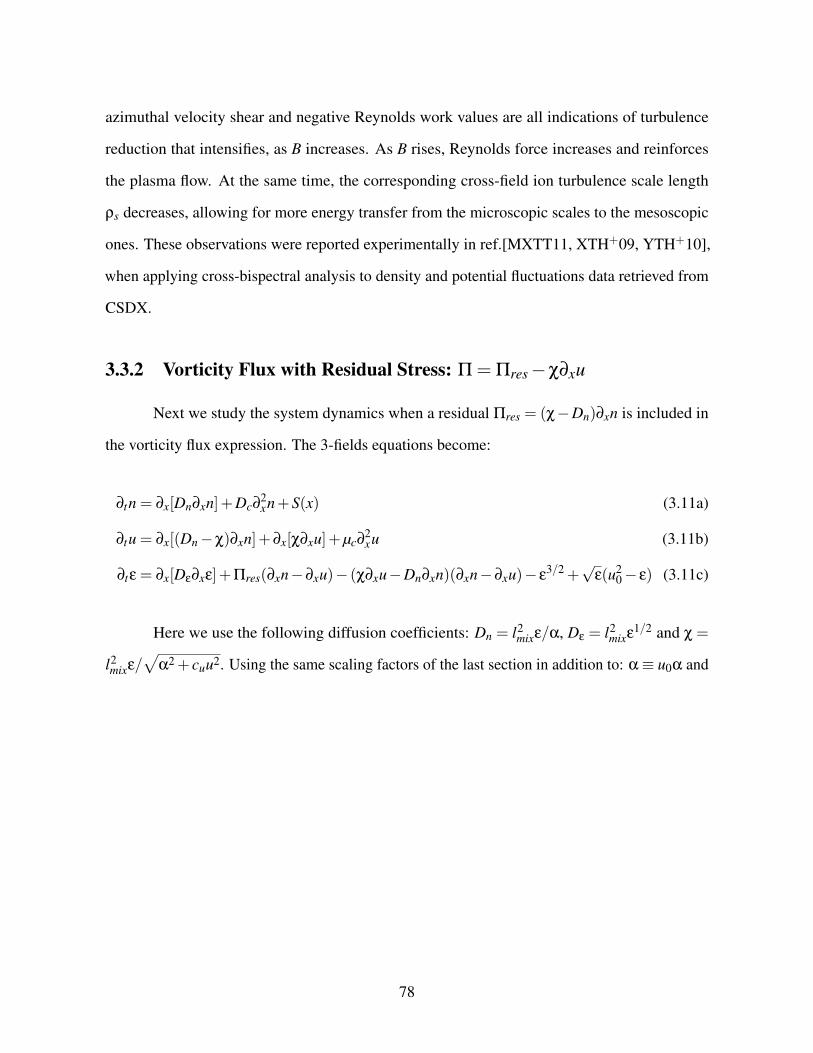
azimuthal velocity shear and negative Reynolds work values are all indications of turbulence
reduction that intensifies, as B increases. As B rises, Reynolds force increases and reinforces
the plasma flow. At the same time, the corresponding cross-field ion turbulence scale length
ρs decreases, allowing for more energy transfer from the microscopic scales to the mesoscopic
ones. These observations were reported experimentally in ref.[MXTT11, XTH+09, YTH+10],
when applying cross-bispectral analysis to density and potential fluctuations data retrieved from
CSDX.
3.3.2 Vorticity Flux with Residual Stress: Π = Πres−χ∂xu
Next we study the system dynamics when a residual Πres = (χ−Dn)∂xn is included in
the vorticity flux expression. The 3-fields equations become:
∂tn = ∂x[Dn∂xn]+Dc∂2xn+S(x) (3.11a)
∂tu = ∂x[(Dn−χ)∂xn]+∂x[χ∂xu]+µc∂2xu (3.11b)
∂tε = ∂x[Dε∂xε]+Πres(∂xn−∂xu)− (χ∂xu−Dn∂xn)(∂xn−∂xu)− ε3/2 +
√ε(u2
0− ε) (3.11c)
Here we use the following diffusion coefficients: Dn = l2mixε/α, Dε = l2
mixε1/2 and χ =
l2mixε/
√α2 + cuu2. Using the same scaling factors of the last section in addition to: α≡ u0α and
78
cu ≡ cu/L2, we obtain the following B-dependent equations:
ωci∂tn = ∂x
[ l20ε2∂xn
ε+ l20(∂x(n−u/ρ2
s ))2
1α+Dc∂xn
]+S (3.12a)
ωci∂tu = ρ2s ∂x
[ l20ε2
ε+ l20(∂x(n−u/ρ2
s ))2
[(
1α− 1√
α2 + cu(u/ρ2s )
2)∂xn
+(1√
α2 + cu(u/ρ2s )
2+µc)∂xu
]](3.12b)
ωci∂tε = ∂x
[ l20ε3/2∂xε
ε+ l20(∂x(n−u/ρ2
s ))2
]+L2
[ l20ε2ρs(∂xn−∂xu/ρ2
s )
ε+ l20(∂x(n−u/ρ2
s ))2)(− 1
α+
1√α2 + cu(u/ρ2
s )2)
−l20ε2
ε+ l20(∂x(n−u/ρ2
s ))2(−∂x
α+
1√α2 + cu(u/ρ2
s )2
∂xuρ2
s)(∂xn− ∂xu
ρ2s)−2ε
3/2 +√
ε
](3.12c)
We show here numerical results that correspond to both Dirichlet and Neumann vorticity
boundary condition at x = 1. Starting with a Dirichlet condition u|x=1 = 0, for an arbitrary case
α = 3 and cu = 6 trial case, numerical results are similar to those obtained when no residual
stress is included in the expression of Π. The steepening of the density profiles, the sheared
azimuthal velocity layer and the negative Reynolds work values in the three left figures of fig.3.8
are all consistent with a global transition that occurs in the plasma as B increases. Variation of
the shearing coefficient cu, which reflects a change in the strength of the flow shear, does not
seem to affect qualitatively the numerical results (right three figures of fig.3.8); the results are
simply insensitive to a change in cu. Therefore we conclude that, while Πres is needed to account
for intrinsic rotation in tokamaks and axial flow generation in linear devices [LDXT16], a state
of enhanced confinement can be recovered using a simple diffusive form of the vorticity flux,
without the need to include a residual stress in the expression for Π.
The scenario of a plasma column surrounded by a layer of fixed neutrals next to the
walls corresponds to a Neumann vorticity boundary condition: ∂u∂x |x=1 = 0. Viscous effects are
79
negligible in this case. We mention here though that the usual experimental case corresponds to
a Dirichlet boundary condition. Steepening of the density profiles, as well as negative Reynolds
work values are recovered as a sign of turbulence suppression, as B increases. The velocity shear,
although present and prominent at the density steepening location, is B independent (top three
figures of fig.3.9). Higher magnetic field values are required for this B-dependence to appear.
The Reynolds work becomes then positive (bottom three figures of fig.3.9). The latter suggests
turbulence production by the flow at high B values, i.e., an instability that might be triggered by
the vorticity gradient at high B instead of being suppressed by the velocity shear.
A change in the mode scale length from l0 = ρs/5 to l0 = 10−3ρs leads to the same
previously mentioned trends of turbulence suppression as indicated by density profile steepening,
negative Reynolds work values and a B dependent sheared azimuthal velocity (see fig.3.10).
More interesting is the relevant case of a higher Prandtl number Pr = µc/Dc = 65000. In
this case, momentum diffusivity dominates the behavior of the plasma characterized by a low
diffusion coefficient Dc. Fig.3.11 shows time evolution of the plasma profiles at consecutive times
t1 and t2. The plasma density builds up at the injection location and the inward flux develops
as a result of density localized concentration, regardless of the magnitude of B. Evidence of a
turbulence suppression such as negative Reynolds work rates and sheared azimuthal velocity are
also recovered.
3.4 Validation Metrics for Model Comparison with Experi-
ment.
Going beyond the simple qualitative comparisons between numerical and experimental
profiles, we propose here a set of quantitative metrics which aim to test whether the adopted model
equations are indeed capable of explaining the experimental observations. Quoting Oberkampf
and Trucano (2002), ”an important issue concerns how comparisons of computational results
80
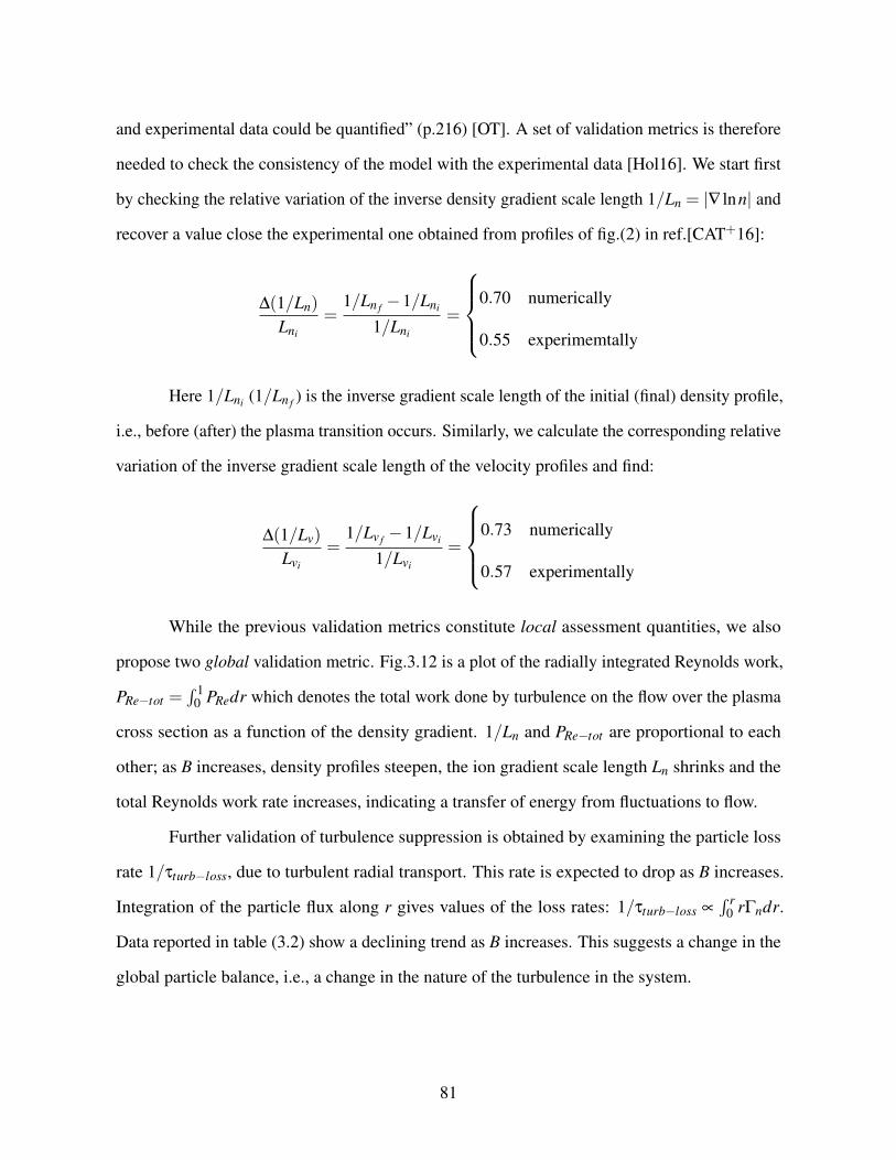
and experimental data could be quantified” (p.216) [OT]. A set of validation metrics is therefore
needed to check the consistency of the model with the experimental data [Hol16]. We start first
by checking the relative variation of the inverse density gradient scale length 1/Ln = |∇ lnn| and
recover a value close the experimental one obtained from profiles of fig.(2) in ref.[CAT+16]:
∆(1/Ln)
Lni
=1/Ln f −1/Lni
1/Lni
=
0.70 numerically
0.55 experimemtally
Here 1/Lni (1/Ln f ) is the inverse gradient scale length of the initial (final) density profile,
i.e., before (after) the plasma transition occurs. Similarly, we calculate the corresponding relative
variation of the inverse gradient scale length of the velocity profiles and find:
∆(1/Lv)
Lvi
=1/Lv f −1/Lvi
1/Lvi
=
0.73 numerically
0.57 experimentally
While the previous validation metrics constitute local assessment quantities, we also
propose two global validation metric. Fig.3.12 is a plot of the radially integrated Reynolds work,
PRe−tot =∫ 1
0 PRedr which denotes the total work done by turbulence on the flow over the plasma
cross section as a function of the density gradient. 1/Ln and PRe−tot are proportional to each
other; as B increases, density profiles steepen, the ion gradient scale length Ln shrinks and the
total Reynolds work rate increases, indicating a transfer of energy from fluctuations to flow.
Further validation of turbulence suppression is obtained by examining the particle loss
rate 1/τturb−loss, due to turbulent radial transport. This rate is expected to drop as B increases.
Integration of the particle flux along r gives values of the loss rates: 1/τturb−loss ∝∫ r
0 rΓndr.
Data reported in table (3.2) show a declining trend as B increases. This suggests a change in the
global particle balance, i.e., a change in the nature of the turbulence in the system.
81
Table 3.2: Particle loss rate 1/τ for increasing B.1/τloss(×10−2) S = 10 S = 50 S = 104
Bblue 1.4 3 1.1Bred 1.2 2.6 0.5
Bblack 0.9 1.8 0.2
3.5 What is the Criterion for Turbulence Suppression?
A conceptual question in modeling drift wave-zonal flow turbulence is the prediction of
when transport barriers are triggered. A variety of proposals are on record. Most are equivalent
to a comparison of linear growth rate to E×B shearing rate (i.e., |γL| vs. |γE×B|). The relevance
of this type of criterion to fully developed turbulence is, at best, unclear. A somewhat non-trivial
criterion [MDG+12], is RT > 1 where:
RT =〈vxvy〉′vE×B
|γe f f |〈v2⊥〉
(3.13)
is the local ratio of the Reynolds power density, to the effective increase in turbulent kinetic energy.
Here |γe f f |(∇n,∇T,VZF) is the turbulence effective growth rate. The idea here is that when
RT > RTcrit (usually RTcrit ∼ 1), the energy transfer to the shear flow exceeds the effective increase
in turbulent kinetic energy, suggesting a collapse of the kθ 6= 0 portion of the turbulence spectrum,
i.e., the part which causes transport. For the model under study here, the instantaneous potential
enstrophy growth rate is |γe f f | = (1/ε).(∂ε/∂t) and 〈v2⊥〉 = εl2
mix = l20ε2/(ε+(l0∇(n− u))2).
Fig.3.13 shows variations of RT with B for this system. Here, RT values are calculated at the
density steepening location and at the turbulent energy saturation time. The proportionality
between B and RT is recovered as anticipated, since an increase in B triggers the formation of
transport barriers.
While the RT > RTcrit criterion is attractive for its extreme simplicity, it suffers from the
facts that: i) |γe f f | is ill-defined, and difficult to calculate, ii) contributions from energy other than
82
the kinetic are ignored. Thus we propose here an alternate criterion, RDT ≥ RDTcrit , where the
global parameter RDT = τrelax/τtrans f er. Here 1/τrelax =−∫
dxΓn∇n/n0, where Γn = 〈vxn/n0〉
is the normalized particle flux, 1/τrelax is the rate of relaxation of the free energy source, which
is ∇n in this model. Of course, ∇n relaxes by exciting drift wave turbulence, so 1/τrelax is
effectively the turbulent enstrophy production rate and would have a connection to the energy
input rate, |γe f f |, used in the RT criterion. Logically then, that should be compared to the rate
of transfer of enstrophy to the mean flow vorticity profile. This may be thought of a turbulent
enstrophy destruction rate, and is closely related to the Reynolds work which appears in RT .
We have then: 1/τtrans f er =−∫
dx〈vxu〉∇u where u = ρ2s ∇2⊥(eφ/Te). Integrating by parts gives:
1/τtrans f er =∫
dx∂x〈vxu〉u so:
RDT =
∫∂x〈vxu〉udx
−∫
Γn∇n/n0dx(3.14)
RDT is manifestly dimensionless and the integrals are calculated along the radius. Noting
the Taylor identity and the fact that u∼ ∇⊥(∇⊥φ)∼ ∇⊥Vy, the correspondence of the numerator
of RDT to that of RT is evident. Finally, given that the potential vorticity is conserved on fluid
particle trajectories, it is not difficult to see the correspondence between fluctuating entropy
(∼ −∫
dv(δ f )2/〈 f 〉) and fluctuating enstrophy. Thus, RDT may be thought of as the ratio of
fluctuation entropy destruction via coupling to the mean flow, to fluctuating entropy production
via relaxation of ∇n. Both numerator and denominator reflect flux-gradient interaction and
both emerge naturally from the formulation of the model, i.e. from expanding the production
term Pprod = (Γn−Π).(∇n−∇u) = Γn∇n+Π∇u−Π∇n−Γn∇u in eq.3.2c. Neglecting the
last two cross terms in Pprod , the numerator and denominator of RDT simply represent the
product of Π and ∇u, and Γn and ∇n respectively. Thus RDT exceeding unity may be thought
of as the simplification of the more general criterion that∫
Pprod passes through zero, i.e.,∫Pprod > 0→
∫Pprod < 0, as the indicator of turbulence collapses. Fig.3.14 shows variations of
RDT with B at the same time and location as for RT . The close relation between RDT and B can
also be interpreted in terms of enstrophy exchange of fluctuations to flow, as B increases. However,
83
the RDT > RDTcrit criterion has a broader and more solid theoretical foundation then RT > RTcrit ,
and easily may be generalized (to more complex models) by expanding the consideration of
potential enstrophy balance. When either RDT or RT exceeds unity, the turbulence levels will
drop and a barrier is likely to be formed. We do not have a proof of either though - particularly
given the ambiguity in just exactly what a barrier is.
3.6 Discussion ans Conclusions.
Features of a CSDX improved confinement are reproduced here using a 1D time-
dependent reduced model. The model recovers the profile evolution in CSDX with an increasing
B, and includes both a slow and a fast time scale: the former corresponding to the time evolution
of the mean fields, and the later corresponding to turbulence production and fast dissipation.
Potential enstrophy is conserved up to dissipation and initial forcing. Inhomogeneous PV mixing
is a central feature here, and occurs on a mixing length that is inversely proportional to the PV
gradient. The use of a mixing length that shrinks as ∇n and ∇u steepen, closes the positive
feedback loop on PV. The model novelty relies in the fact that it reduces the profiles evolution to
only two fluxes: a vorticity and a density flux.
Numerical solutions agree with the experimental findings, and show: a steepening of the
density profile, a reinforced E×B sheared layer, an increased Reynolds work and a reduction
in the turbulence and particle transport, as B increases. Numerical solutions also show that the
steepening of ∇n is recovered without the use of an off-diagonal term nVpinch in the expression
of the particle flux Γn. The experimentally apparent inward flux is simply of diffusive nature at
high B. Moreover, the model predicts qualitatively similar results, with or without the inclusion
a residual stress Πres in the vorticity flux expression Π. We conclude then the following: both
density and vorticity fluxes have purely diffusive forms: Γn = −∂xn and Π = −∂xu, where u
is the vorticity. The inward pinch Vpinch and residual stress Πres necessary to drive axial flows
84
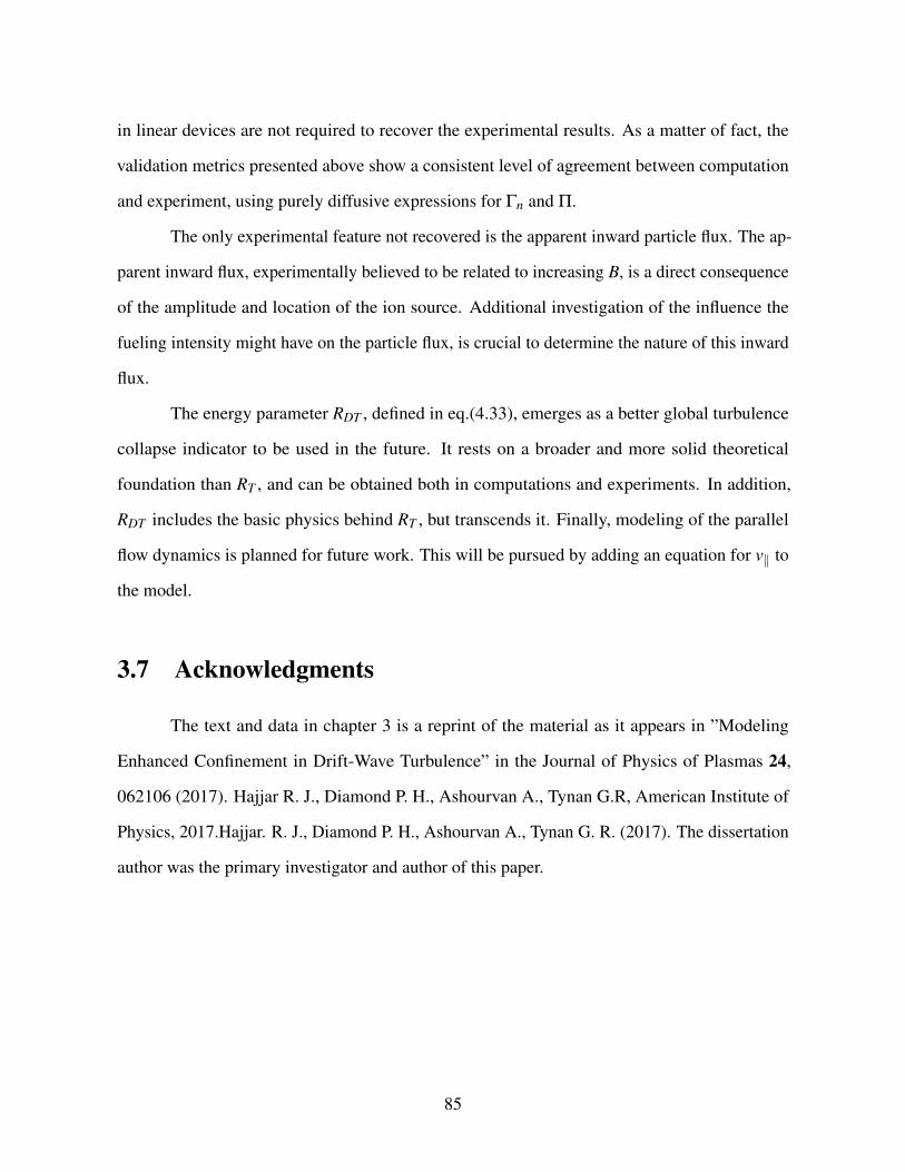
in linear devices are not required to recover the experimental results. As a matter of fact, the
validation metrics presented above show a consistent level of agreement between computation
and experiment, using purely diffusive expressions for Γn and Π.
The only experimental feature not recovered is the apparent inward particle flux. The ap-
parent inward flux, experimentally believed to be related to increasing B, is a direct consequence
of the amplitude and location of the ion source. Additional investigation of the influence the
fueling intensity might have on the particle flux, is crucial to determine the nature of this inward
flux.
The energy parameter RDT , defined in eq.(4.33), emerges as a better global turbulence
collapse indicator to be used in the future. It rests on a broader and more solid theoretical
foundation than RT , and can be obtained both in computations and experiments. In addition,
RDT includes the basic physics behind RT , but transcends it. Finally, modeling of the parallel
flow dynamics is planned for future work. This will be pursued by adding an equation for v‖ to
the model.
3.7 Acknowledgments
The text and data in chapter 3 is a reprint of the material as it appears in ”Modeling
Enhanced Confinement in Drift-Wave Turbulence” in the Journal of Physics of Plasmas 24,
062106 (2017). Hajjar R. J., Diamond P. H., Ashourvan A., Tynan G.R, American Institute of
Physics, 2017.Hajjar. R. J., Diamond P. H., Ashourvan A., Tynan G. R. (2017). The dissertation
author was the primary investigator and author of this paper.
85
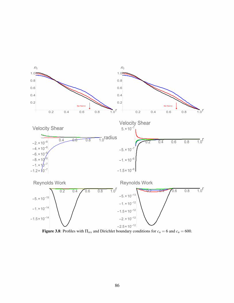
0.2 0.4 0.6 0.8 1.0r
0.2
0.4
0.6
0.8
1.0
ni
Ion Source
0.2 0.4 0.6 0.8 1.0r
0.2
0.4
0.6
0.8
1.0
ni
Ion Source
0.4 0.6 0.8 1.0radius
-1.2×10⁻⁷-1.×10-7-8.×10-8-6.×10-8-4.×10-8-2.×10-8
Velocity Shear
0.2 0.4 0.6 0.8 1.0r
-1.5×10⁻⁶
-1.×10-6
-5.×10-7
5.×10-7Velocity Shear
0.2 0.4 0.6 0.8 1.0r
-1.5×10⁻¹⁴
-1.×10-14
-5.×10-15
Reynolds Work
0.2 0.4 0.6 0.8 1.0r
-2.5×10⁻¹²
-2.×10-12
-1.5×10⁻¹²
-1.×10-12
-5.×10-13
Reynolds Work
Figure 3.8: Profiles with Πres and Dirichlet boundary conditions for cu = 6 and cu = 600.
86
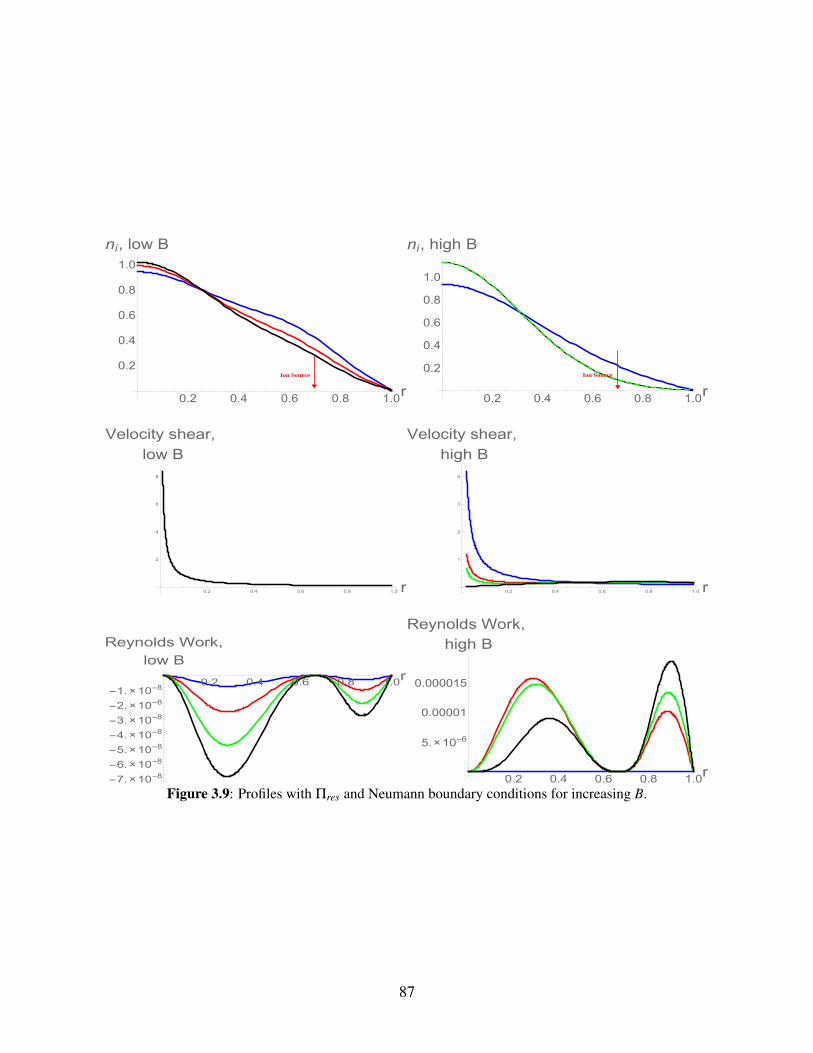
0.2 0.4 0.6 0.8 1.0r
0.2
0.4
0.6
0.8
1.0
ni, low B
Ion Source
0.2 0.4 0.6 0.8 1.0r
0.2
0.4
0.6
0.8
1.0
ni, high B
Ion Source
0.2 0.4 0.6 0.8 1.0 r
2
4
6
8
Velocity shear,
low B
0.2 0.4 0.6 0.8 1.0 r
1
2
3
4
Velocity shear,
high B
0.2 0.4 0.6 0.8 1.0r
-7.×10-8-6.×10-8-5.×10-8-4.×10-8-3.×10-8-2.×10-8-1.×10-8
Reynolds Work,
low B
0.2 0.4 0.6 0.8 1.0r
5.×10-6
0.00001
0.000015
Reynolds Work,
high B
Figure 3.9: Profiles with Πres and Neumann boundary conditions for increasing B.
87
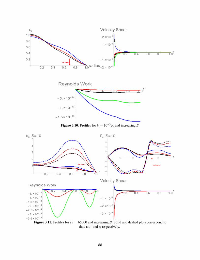
0.2 0.4 0.6 0.8 1.0radius
0.2
0.4
0.6
0.8
1.0
ni
Ion Source
0.2 0.4 0.6 0.8 1.0r
-2.×10-8
-1.×10-8
1.×10-8
2.×10-8
Velocity Shear
0.2 0.4 0.6 0.8 1.0r
-1.5×10⁻¹³
-1.×10-13
-5.×10-14
Reynolds Work
Figure 3.10: Profiles for l0 = 10−3ρs and increasing B.
0.2 0.4 0.6 0.8 1.0r
1
2
3
4
5ni, S=10
Ion Source
0.2 0.4 0.6 0.8 1.0 r
-0.06
-0.04
-0.02
0.02
0.04
0.06
Γi, S=10
Ion Source
0.2 0.4 0.6 0.8 1.0r
-3.5×10⁻¹⁴-3.×10-14
-2.5×10⁻¹⁴-2.×10-14
-1.5×10⁻¹⁴-1.×10-14-5.×10-15
Reynolds Work
0.2 0.4 0.6 0.8 1.0r
-3.×10-8
-2.×10-8
-1.×10-8
Velocity Shear
Figure 3.11: Profiles for Pr = 65000 and increasing B. Solid and dashed plots correspond todata at t1 and t2 respectively.
88
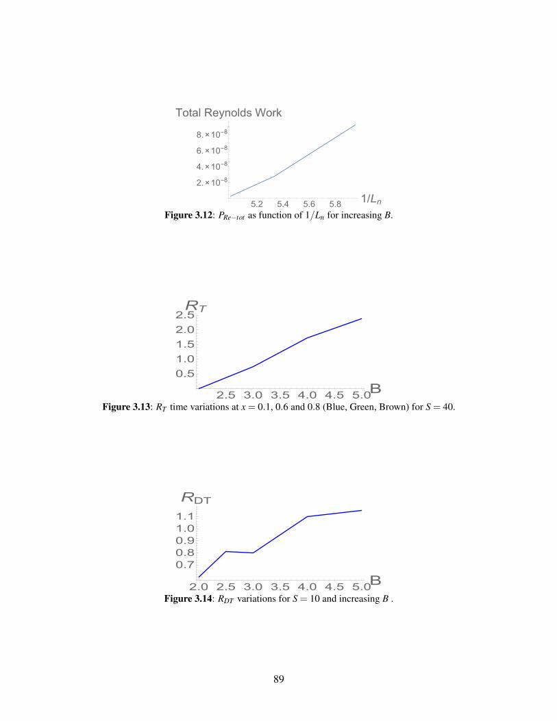
5.2 5.4 5.6 5.8 1/Ln
2.×10-8
4.×10-8
6.×10-8
8.×10-8
Total Reynolds Work
Figure 3.12: PRe−tot as function of 1/Ln for increasing B.
2.5 3.0 3.5 4.0 4.5 5.0B0.5
1.0
1.5
2.0
2.5RT
Figure 3.13: RT time variations at x = 0.1, 0.6 and 0.8 (Blue, Green, Brown) for S = 40.
2.0 2.5 3.0 3.5 4.0 4.5 5.0B0.70.80.91.01.1
RDT
Figure 3.14: RDT variations for S = 10 and increasing B .
89
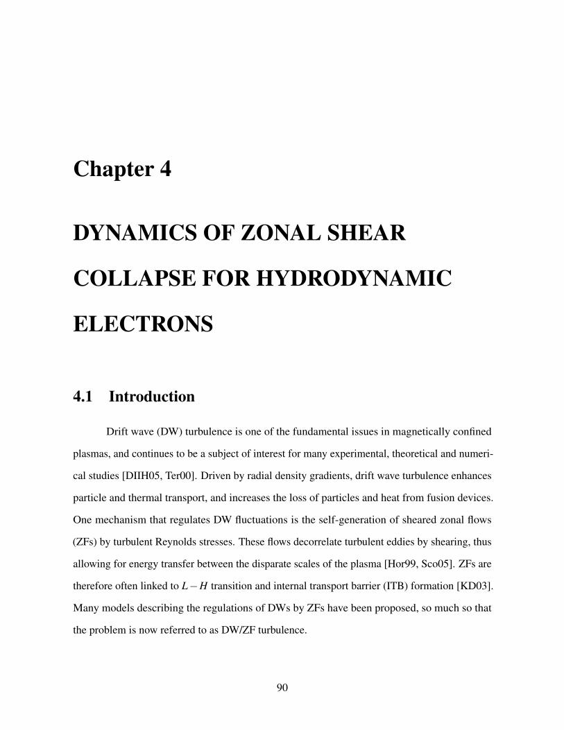
Chapter 4
DYNAMICS OF ZONAL SHEAR
COLLAPSE FOR HYDRODYNAMIC
ELECTRONS
4.1 Introduction
Drift wave (DW) turbulence is one of the fundamental issues in magnetically confined
plasmas, and continues to be a subject of interest for many experimental, theoretical and numeri-
cal studies [DIIH05, Ter00]. Driven by radial density gradients, drift wave turbulence enhances
particle and thermal transport, and increases the loss of particles and heat from fusion devices.
One mechanism that regulates DW fluctuations is the self-generation of sheared zonal flows
(ZFs) by turbulent Reynolds stresses. These flows decorrelate turbulent eddies by shearing, thus
allowing for energy transfer between the disparate scales of the plasma [Hor99, Sco05]. ZFs are
therefore often linked to L−H transition and internal transport barrier (ITB) formation [KD03].
Many models describing the regulations of DWs by ZFs have been proposed, so much so that
the problem is now referred to as DW/ZF turbulence.
90
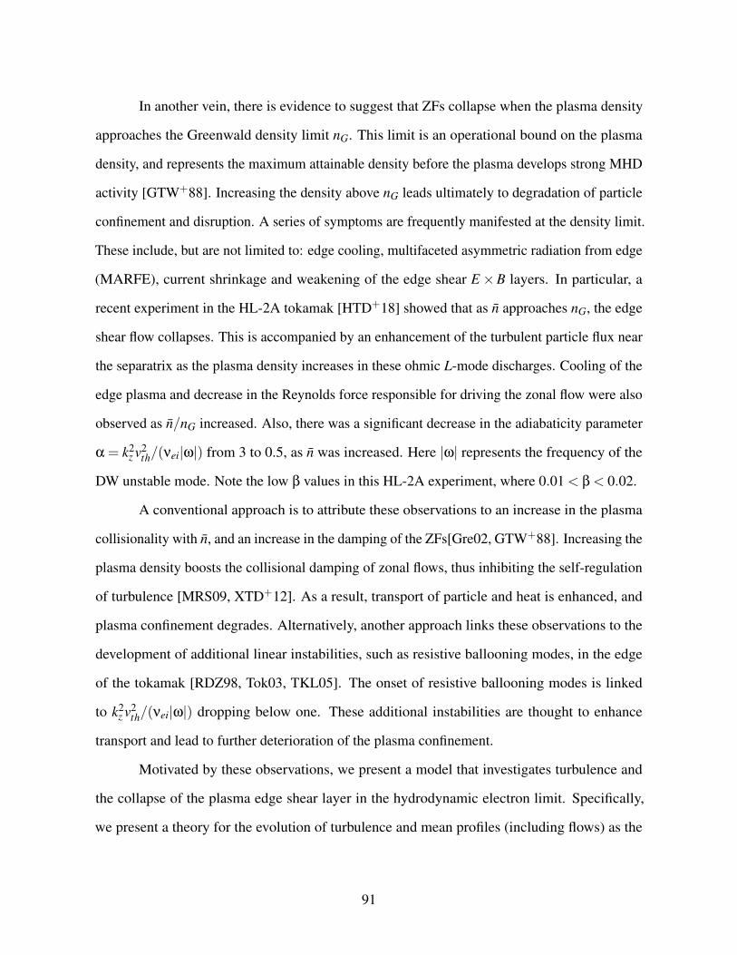
In another vein, there is evidence to suggest that ZFs collapse when the plasma density
approaches the Greenwald density limit nG. This limit is an operational bound on the plasma
density, and represents the maximum attainable density before the plasma develops strong MHD
activity [GTW+88]. Increasing the density above nG leads ultimately to degradation of particle
confinement and disruption. A series of symptoms are frequently manifested at the density limit.
These include, but are not limited to: edge cooling, multifaceted asymmetric radiation from edge
(MARFE), current shrinkage and weakening of the edge shear E×B layers. In particular, a
recent experiment in the HL-2A tokamak [HTD+18] showed that as n approaches nG, the edge
shear flow collapses. This is accompanied by an enhancement of the turbulent particle flux near
the separatrix as the plasma density increases in these ohmic L-mode discharges. Cooling of the
edge plasma and decrease in the Reynolds force responsible for driving the zonal flow were also
observed as n/nG increased. Also, there was a significant decrease in the adiabaticity parameter
α = k2z v2
th/(νei|ω|) from 3 to 0.5, as n was increased. Here |ω| represents the frequency of the
DW unstable mode. Note the low β values in this HL-2A experiment, where 0.01 < β < 0.02.
A conventional approach is to attribute these observations to an increase in the plasma
collisionality with n, and an increase in the damping of the ZFs[Gre02, GTW+88]. Increasing the
plasma density boosts the collisional damping of zonal flows, thus inhibiting the self-regulation
of turbulence [MRS09, XTD+12]. As a result, transport of particle and heat is enhanced, and
plasma confinement degrades. Alternatively, another approach links these observations to the
development of additional linear instabilities, such as resistive ballooning modes, in the edge
of the tokamak [RDZ98, Tok03, TKL05]. The onset of resistive ballooning modes is linked
to k2z v2
th/(νei|ω|) dropping below one. These additional instabilities are thought to enhance
transport and lead to further deterioration of the plasma confinement.
Motivated by these observations, we present a model that investigates turbulence and
the collapse of the plasma edge shear layer in the hydrodynamic electron limit. Specifically,
we present a theory for the evolution of turbulence and mean profiles (including flows) as the
91
adiabaticity parameter α decreases below unity that is, as the plasma response passes from the
adiabatic limit (α 1) to the hydrodynamic limit (α 1). Interestingly enough, findings of this
paper are easily applicable to the density limit experiments since α ∝ 1/n. A particularly simple
model proposed by Hasegawa and Wakatani describes the dynamics of two-dimensional (2D)
edge drift wave turbulence in a collisional plasma in the presence of a constant magnetic field.
This generic system of equations describes the excitation and damping of unstable modes in
terms of a few collisionality parameters, leading to a stationary turbulence level without external
drive. In particular, the Hasegawa-Wakatani system of equations remains a valid model for edge
turbulence dynamics, regardless of the magnitude of the plasma β. Although multiple studies
investigating the characteristics of turbulence in the hydrodynamic limit have been published,
no explanation of why the shear flow collapses and/or why drift wave turbulence is enhanced
for α < 1 was presented. In fact, most studies of ZF behavior in the hydrodynamic electron
regime simply repeat numerical results that show strong turbulence and weak zonal flows in
the hydrodynamic limit [KT13, NBD07, CBS95, PBN13], and verify the usual power laws of
turbulent energies in this limit [GG15]. Note that for the parameters of the HL-2A experiments,
it is quite unlikely that resistive ballooning modes are excited.
This paper addresses these questions by presenting a simple reduced model for transport
enhancement and weakening of the edge shear layer in the hydrodynamic electron limit. The
model is derived from the Hasegawa-Wakatani (HW) equations for collisional drift waves, and
self-consistently studies space and time evolution of the mean density n, mean azimuthal flow
vy and turbulent potential enstrophy ε. The model determines the role of the Reynolds stress
〈vxvy〉 in the feedback loop between flows and turbulence, and gives additional insight into the
DW/ZF relation in the hydrodynamic electron limit. Quasi-linear analysis shows that both the
particle flux Γn and the turbulent viscosity χy are enhanced as α decreases. However, the residual
vorticity stress Πres, which accelerates the flow, is reduced with α. The mean vorticity gradient
equal to Πres/χy is then reduced, and the edge shear layer collapses. As a result, transport
92
of particles and heat increases. These findings are relevant to the density limit experiment,
as α ∝ 1/n. When n increases, α decreases, and Πres/χy is reduced. The plasma production
of zonal flows declines and turbulence and transport increase. Thermal and particle transport
increase, thereby triggering cooling of the edge plasma, in part because of inward turbulence
spreading. For constant pressure, a drop in plasma temperature Te leads to further increase in the
density and feedback loop between Te and n forms.
The rest of the paper is organized as follows: Section (4.2) gives the linear response
analysis of the basic Hasegawa-Wakatani system, as well as solution of the DW dispersion
relation in both the adiabatic and hydrodynamic limits. Section (4.3) introduces the reduced
model used to describe the evolution of the three fields: n, vy and ε. In Section (4.4), we calculate
the expressions for the particle flux, the vorticity flux and the Reynolds work in both adiabatic and
hydrodynamic limits. The latter reflects the potential enstrophy exchange between fluctuations
and mean flow. The model is then simplified to a predator/prey model by slaving the expression
for ε in the equations for n and vy in Section (4.5). Section (4.6) gives a physical argument as to
why zonal flow formation is weak in the hydrodynamic limit. Variations of the mean vorticity
gradient Πres/χy, as well as changes in the scaling of the vorticity flux 〈vx∇2⊥φ〉 are examined,
in order to characterize the mesoscopic plasma response as α decreases. The drop in zonal flow
drive is reconciled with the persistence of potential vorticity mixing in the hydrodynamic limit.
Section (4.7) interprets the experimental observations obtained in the density limit experiment
from the perspective of the collapse of ZFs in the hydrodynamic electron limit. A scenario
linking shear layer collapse to the density limit is proposed. Finally, conclusions and future work
are discussed in Section (4.8).
93
4.2 Basic System and Linear Stability Analysis
In a box of dimensions: 0≤ x≤ Lx, 0≤ y≤ Ly, 0≤ z≤ Lz, the equations for the density
n and vorticity ∇2φ in a nonuniform plasma with density n0(x) and constant magnetic field
B = Bz are [HW83]:
dndt
=−v2
thνei
∇2‖(φ−n)+D0∇
2n (4.1a)
d∇2φ
dt=−
v2th
νei∇
2‖(φ−n)+µ0∇
2(∇2φ) (4.1b)
Here the fields are normalized as: n ≡ n/n0, φ ≡ eφ/Te, t ≡ ωcit, length ≡ length/ρs,
vth ≡ vth/cs and νei ≡ νei/ωci. The average plasma density, the electron temperature and thermal
velocity, as well as the plasma sound speed are n0, Te, vth and cs respectively. ωci is the
ion cyclotron frequency, and ρs = cs/ωci is the ion Larmor radius with temperature Te. The
collisional diffusion coefficients D0 and µ0 dissipate energy at small scales by frictional drag
through forward energy cascade. The electron parallel diffusion rate α =−v2th∇2‖/νei = k2
z v2th/νei
couples the vorticity fluctuations to those in the density profile. The convective derivative is equal
to: d/dt = ∂t +(z×∇φ).∇ = ∂t + vE .∇ where vE is the E×B drift. The fields are decomposed
into a perturbation and a zonally averaged part: f = f (x, t)+ f (x,y,z, t), where the averaging is
preformed over the directions of symmetry y and z:
〈 f 〉= f =1
LyLz
∫ Ly
0
∫ Lz
0f dydz
94
Equations for the density and vorticity fluctuations are written as:
∂t n+ vx.∇n =−v2
thνei
∇2‖(φ− n)−φ, n+D0∇
2n (4.2a)
∂t∇2φ+ vx.∇∇2φ =−
v2th
νei∇
2‖(φ− n)−φ,∇2
φ+µ0∇2(∇2
φ) (4.2b)
Here the mean flow shear ∇2φ in eq.(4.2b) is self-generated by the Reynolds stress 〈vxvy〉, and
is driven by the DW interactions. Based in the triad coupling, this internal shear results from
nonlinear energy transfer related, but not identical to, the inverse energy cascade in a 2D fluid.
The nonlinear advection terms are expressed as Poisson brackets: f ,g= ∂x f ∂yg−∂y f ∂xg and
represent spatial scattering of the fluctuation energy.
In the Hasegawa-Wakatani (HW) system, the plasma response and the character of the
flow are mainly determined by three parameters: the collisional diffusion coefficients D0 and
µ0, and the adiabaticity parameter α = k2z v2
th/(νei|ω|). While D0 and µ0 regulate the dissipation
of energy at small scales, α determines the efficiency of zonal flow production, and controls
its mescocopic response. Defined as the ratio between the parallel diffusion rate and the drift
frequency, α controls the phase difference between φ and n, and thus the transport. When
α > 1, the plasma response is near adiabatic, φ and n are closely coupled, and n ' φ. The
Hasegawa-Wakatani system effectively reduces then to the Hasegawa-Mima equation [HM77],
with a phase shift between n and φ. In the opposite limit however, α < 1, the plasma response is
said to be hydrodynamic. Eqs.(4.2a-4.2b) are then weakly coupled, and the n dynamics resemble
that of a passive scalar. Moreover, the vorticity equation tends toward that for a 2D Navier-Stokes
fluid [CBS95].
For a linear stability analysis of the HW equations, we write the fluctuation fields
as: fm = δ fm(x)ei[kmy+kzz−ωt] with ω = ωr + i|γm|. Here ωr, |γm|, km and kz are the linear
eigenfrequency, the growth rate, the azimuthal and the parallel wavenumbers of the unstable
95
mode respectively. The drift wave dispersion relation is then:
ω2 + i
α
k2⊥ρ2
s
[ω(1+ k2
⊥ρ2s )−ω
?]= 0 (4.3)
where ω? = km|vd|=−kmρscs∇n > 0 is the electron drift frequency, and vd = ρscs∇n < 0 is the
electron diamagnetic drift velocity. The solution of eq.(4.3) is given by:
ω =12
(− i
α(1+ k2⊥ρ2
s )
k2⊥ρ2
s+
√4iω?α
k2⊥ρ2
s−(
α(1+ k2⊥ρ2
s )
k2⊥ρ2
s
)2)
(4.4)
This expression is simplified, according to the magnitude of α/|ω|, i.e., the magnitude of
α.
In the adiabatic limit: (α 1 and α |ω|)
When the parallel diffusion rate k2z v2
th/νei is larger than both the drift frequency |ω| and
the electron diamagnetic frequency |ω?|, eq.(4.4) reduces to:
ωadiabatic =ω?
1+ k2⊥ρ2
s+ i
ω?2k2⊥ρ2
s
α(4.5)
In the adiabatic limit, ωr does not depend on α. However, the growth rate |γm| is proportional
to 1/α. For large α, the growth rate is |γm| 1, and the drift wave eigenfrequency is simply
written as:
ωadiabatic ' ωr = ω
?(1+ k2⊥ρ
2s )−1 (4.6)
In the hydrodynamic limit: (α 1 and α |ω|)
When the parallel diffusion rate k2z v2
th/νei is much smaller than |ω|, the expression for
the frequency reads:
ωhydrodynamic '12
(− i
α(1+ k2⊥ρ2
s )
k2⊥ρ2
s+
√4iαω?
k2⊥ρ2
s
)'
√ω?α
2k2⊥ρ2
s(1+ i) (4.7)
96
In this limit, the growth rate and the real part are both equal to: ωr = |γm|=√
ω?α/2k2⊥ρ2
s . In
contrast to the adiabatic limit, the contribution of |γm| cannot be neglected in the expression for
ωhydrodynamic.
A comparison of eq.(4.6) and eq.(4.7) shows that ωadiabatic is dominantly real, while
ωhydrodynamic involves a comparable real and imaginary part. While the motion of the drift
waves is purely oscillatory in the adiabatic limit, in the hydrodynamic limit, the dynamics of the
perturbation resembles that of a convective cell. This feature dictates the behavior of the flow in
the two plasma regimes.
4.3 Reduced Model
4.3.1 The equations
In this section, a 1D reduced model that self-consistently describes the evolution of
turbulence and plasma profiles is presented. The equations relating the time and space evolution
of the plasma mean density n, and mean vorticity ∇2φ are obtained by averaging eqs.(4.1a-4.1b)
over the directions of symmetry:
∂t n =−∂x〈vxn〉+D0∇2n (4.8a)
∂t∇2φ =−∂x〈vx∇2φ〉−νin(vy− vn)+µ0∇
2∇2φ (4.8b)
A neutral damping term proportional to the ion-neutral collision frequency νin ∝ nn, is
added to the mean vorticity equation. This term can be significant at the plasma edge. It is a sink
of energy transfered to larger scales, and so damps the zonal flows. The neutral friction can be
dropped from the mean vorticity equation if νin→ 0, i.e., for low neutral density nn.
In addition to eqs.(4.8a-4.8b), we formulate an equation for the fluctuation potential
enstrophy ε = 〈(n−∇2φ)2/2〉. The HW system locally conserves the potential vorticity defined
97
as q = n−∇2φ, up to viscosity and particle diffusivity. A linearized equation describing the time
evolution of the turbulent potential vorticity q = n−∇2φ is obtained by subtracting eq.(4.2b)
from eq.(4.2a):∂q∂t
+ vx.∇q =−φ, q+µ0∇2q =⇒ dq
dt= µ0∇
2q (4.9)
where q = q+ q, and µ0 and D0 are assumed to be of the same order. Eq.(4.9) represents a
conservation of the total potential vorticity up to viscous dissipation. Therefore, the potential
enstrophy ε = 〈q2〉/2 = 〈(n−∇2φ)2〉/2 is also conserved up to collisional diffusion. This can
be shown by multiplying eq.(4.9) by q = n−∇2φ, and performing a zonal integral. Detailed
calculations can be found in ref. [HDAT17, ADG16, AD16]. Here we simply write the time
evolution equation for the potential enstrophy ε:
∂tε+∂xΓε =−(Γn−Π)(∂xn−∂xxvy)− ε3/2 +P (4.10)
In eq.(4.10), Γn and Π are the particle and vorticity flux respectively, while ∂xn and
∂xxvy are the mean density and mean vorticity gradients respectively. The diffusive energy flux
Γε on the LHS is the mesoscopic spreading of turbulence due to the three wave coupling. It
represents local diffusion of the potential enstrophy ε. The potential enstrophy flux is written
as: Γε =−Dε∂xε =−l2mix√
ε∂xε, where lmix = vxτc is the turbulent mixing length and τc is the
turbulence correlation time. The first term on the RHS of eq.(4.10) accounts for direct mean
flow-fluctuation coupling, and converts the mean potential enstrophy into fluctuation potential
enstrophy. This coupling term relates variations of the turbulent potential enstrophy to those in
the mean profile of n and vy, via the particle flux Γn = 〈vxn〉 and the vorticity flux Π = 〈vx∇2φ〉.
The second term on the RHS of eq.(4.10) dissipates the fluctuation potential enstrophy at a rate√
ε. This dissipation is due to the collisional coefficients D0 and µ0. Lastly, the production term P
represents an input of the potential enstrophy due to linear growth, driven by the mean profiles. It
is proportional to ε and linear in γDW , the growth rate of the DW instability: P = γDW ε. Dropping
98
the neutral damping term from the vorticity equation, as well as the ¯. . . sign, we simplify the
notation by writing u = ∇2φ to obtain:
∂tn =−∂xΓn +D0∇2n (4.11a)
∂tu =−∂xΠ+µ0∇2u (4.11b)
∂tε+∂xΓε =−(Γn−Π)(∂xn−∂xu)− ε3/2 +P (4.11c)
Written in 1D (in radius), this system models the evolution of DW intensity and the formation of
zonal flows in the plasma. For this purpose, an expression for the mixing length lmix is required.
One approach consists of considering a mixing length that exhibits a turbulence suppression
through the azimuthal shear u = ∇vy:
lmix =l0(
1+(l0∇u)2
ε
)δ(4.12)
where δ is a free parameter and l0 is an external dynamical turbulence production scale length.
Eq.(4.12) exhibits a decorrelation of the turbulent structures by the flow shear u = ∇vy [BDT90]:
when the flow shear increases, the mixing length decreases. When lmix is reduced, the production
of potential enstrophy ε also drops, the mean profiles steepen, and a closed feedback loop is
obtained. In the particular case of weak or collapsed flow shear, u = ∇vy ' 0 so a constant
mixing length lmix ' l0 results.
4.4 Expressions for the Turbulent Fluxes
In addition to the expression for lmix, expressions for the turbulent fluxes 〈vxn〉 and 〈vxvy〉
are needed to close the model and solve eqs.(4.11a-4.11c). In this section, we use quasi linear
theory to calculate the expressions for the particle flux and vorticity flux.
99
4.4.1 The Particle Flux: 〈nvx〉
To calculate the expression for the particle flux 〈nvx〉, we write the electron density
fluctuation as n = φ+ h, where h is the deviation from the adiabatic response. Plugging in
eq.(4.2a), we obtain:
h =ω?−ω
ω+ iαφ, n = φ+h =
(ω?+ iαω+ iα
)φ
In the adiabatic limit, ω' ω? and the following relation between n and φ is recovered:
n =(
1− i(ω?−ω)/α
)φ' φ [LDXT16]. For vx =−ikmρscsδφ, the expression for the particle
flux 〈nvx〉 is:
Γn =−[(α+ |γm|)|ω+ iα|2
d lnndx
+αωr
kmρscs|ω+ iα|2]〈δv2
x〉
' −(α+ |γm|)|ω+ iα|2
d lnndx〈δv2
x〉
=−Dn0
dndx
(4.13)
The particle diffusion coefficient is: D =[(α+ |γm|)/|ω+ iα|2
]〈δv2
x〉. The expression
for the particle diffusion coefficient D depends on α, and changes as the plasma passes from the
adiabatic to the hydrodynamic regime. We introduce next the factor f that represents the fraction
of the fluctuation energy εl2mix which is in the kinetic energy of radial motion:
〈δv2x〉= f εl2
mix =〈δv2
x〉〈δn2〉+ 〈δv2
x〉εl2
mix (4.14)
100
Using the expressions for n and vx, the expression for f is equal to:
f =k2⊥ρ2
s∣∣∣ω∗+ iαω+ iα
∣∣∣2 + k2⊥ρ2
s
=
k2⊥ρ2
s
1+ k2⊥ρ2
s, in the adiabatic regime
1|ω∗/α|+1
, in the hydrodynamic regime(4.15)
In the adiabatic regime, the kinetic energy 〈δv2x〉 is less then 〈δn2〉, and the electron
total energy is mostly thermal/internal energy. Therefore, the factor f 1. However, in the
hydrodynamic regime, the kinetic energy of the electrons rises as compared to 〈δn2〉, reflecting
an increase in the screening of ion diamagnetic oscillations such that f → 1. For small values of
k2⊥ρ2
s 1, the two limits of f are:
f → k2
⊥ρ2s ' 0, in the adiabatic regime
f → 1, in the hydrodynamic regime
Finally, for purely adiabatic DWs, the relation 〈δv2x〉 ' k2
⊥ρ2s εl2
mix is recovered.
4.4.2 The Vorticity Flux: 〈vx∇2⊥φ〉
In addition to Γn, we calculate the vorticity flux Π = 〈vx∇2⊥φ〉. This flux relates to the
Reynolds force that controls the relation between turbulence and zonal flows via the Taylor
identity: −∂x〈vxvy〉 = 〈vx∇2⊥φ〉. The Taylor identity directly links the zonal flow momentum
conservation to potential enstrophy balance [DGH+08]. To calculate Π, we use the vorticity
equation and drop the neutral drag term, as it is significant only at the edge. The vorticity flux
101
then follows as:
Π = ∑m−k2
mρ2s c2
s |γm||ω|2
|φ2|d2vy
dx2 +2Re[kmρscsα
ω
(ω?−ω
ω+ iα
)|φ|2]
=−χyd〈∇2
⊥φ〉dx
+Πres
=−χyd2vy
dx2 +Πres
(4.16)
The first term of eq.(4.16) represents the diffusive flux, while the second term is the
residual stress, i.e., the non-diffusive flux driven by ∇n. The turbulent viscosity χy relating the
mean vorticity gradient d(∇vy)/dx to the vorticity flux Π is equal to:
χy = ∑m
k2mρ2
s c2s |γm|
|ω|2|φ2|= |γm|〈δv2
x〉|ω|2
(4.17)
Here χy depends on the adiabaticity parameter, as both |γm| and |ω| are α-dependent.
The residual stress Πres resulting from coupling between the density and vorticity profiles
is equal to:
Πres =
kmρscsωciα[(ωr)2(ω?−ωr)−|γm|2(ωr +ω?)−ω?α|γm|
]|ω|2×|ω+ iα|2
〈φ2〉 (4.18)
Πres converts the driving particle flux into zonal (azimuthal) flow, and accelerates vy from
rest. Similar to the expression for χy, Πres varies as α changes, affecting thereby the character
of the flow in both plasma limits. In the adiabatic limit, an examination of the expression
for Πres shows that the residual stress is inversely proportional to α, i.e., Πresadia ∝ 1/α. In the
hydrodynamic limit however, the residual stress is directly proportional to√
α, i.e. Πreshydro ∝
√α,
for α 1.
102
4.4.3 Fluxes and Reynolds Work in Adiabatic and Hydrodynamic Limits.
The expressions for the particle and vorticity flux can be simplified depending on the
value of α, i.e., depending on the electron plasma response.
In the adiabatic limit: (α |ω|)
In this limit, α 1. The growth rate |γm| ' 1/α 1, and |ω|2 ' (ωr)2 =[ω?/(1+
k2⊥ρ2
s )]2
. The expressions for the particle and vorticity fluxes in the adiabatic limit are:
n0Γn =−〈δv2
x〉α
dndx'−εl2
mixα
dndx
(4.19a)
Π =−|γm|〈δv2x〉
|ω|2d2vy
dx2 −ωci〈δv2
x〉α
dndx
( k2⊥ρ2
s
1+ k2⊥ρ2
s
)'−εl2
mixα
d2vy
dx2 −ωciεl2
mixα
dndx
(4.19b)
Here 〈δv2x〉adiabatic = fadiabaticεl2
mix = k2⊥ρ2
s εl2mix/(1+k2
⊥ρ2s ). Scalings of the particle flux
Γn, the turbulent viscosity χy and the residual stress Πres in the adiabatic limit are:
Γn '−(εl2mix/α)∇n (4.20a)
χy ' εl2mix/α (4.20b)
Πres '−(ωciεl2
mix/α)∇n (4.20c)
Here, Γn, χy and Πres are all inversely proportional to α In addition, both Γn and Πres
are proportional to ∇n. The expression for the Reynolds power density PRe that represents the
power exerted by the turbulence on the flow vy, is obtained by multiplying the Reynolds force
FRe =−∂x〈vxvy〉 by the azimuthal flow vy. In the adiabatic limit, PRe is equal to:
PRe =−∂x〈vxvy〉vy '(− ε
α
d2vy
dx2 −ωciε
α
dndx
)vyl2
mix (4.21)
103
In the (likely case of) absence of an external azimuthal momentum source, and for a
vanishing Reynolds power density PRe = 0, the mean vorticity gradient is independent of α and
is given by:d2vy
dx2 =Πres
χy=−ωci
dndx
(4.22)
In the hydrodynamic limit: (α |ω|)
For ωr = |γm| =√
ω?α/(2k2⊥ρ2
s ), expressions for the particle and vorticity fluxes are
equal to:
n0Γn '−
√k2⊥ρ2
s
2kmρscs
√|dn/dx|
α〈δv2
x〉 ' −εl2
mix√α|ω?|
dndx
(4.23a)
Π =−|γm|〈δv2x〉
|ω|2d2vy
dx2 −ωci〈δv2
x〉kmρscs
.
√k2⊥ρ2
s
2
√α
|ω?|
' − εl2mix√
α|ω?|d2vy
dx2 −ωciε√
αl2mix
|ω?|3/2dndx
(4.23b)
Here we used 〈δv2x〉hydrodynamic = fhydrodynamicεl2
mix = εl2mix/
[|ω∗/α|+1
]< εl2
mix. Scal-
ings of the turbulent fluxes are then:
Γn '−(εl2mix/
√α|ω?|)∇n (4.24a)
χy ' εl2mix/
√α|∇n| (4.24b)
Πres '−(ωciε
√αl2
mix/|ω?|3/2)∇n (4.24c)
While Γn and χy are inversely proportional to√
α in the hydrodynamic limit, the residual
stress Πres scales proportionally with√
α. We note here that in the hydrodynamic limit, the
particle flux Γhydron is proportional to
√|∇n|, and the residual stress Πres
hydro is proportional to
1/√|∇n|. Such superficially unusual scalings with |∇n| result from neglecting the contributions
104
of the diffusive damping related to D0 and µ0 in the density and vorticity equations, while
performing the linear analysis. Obviously these should not be extrapolated to regimes of very
weak ∇n drive. In the hydrodynamic limit, the Reynolds power density is equal to:
PRe =−∂x〈vxvy〉vy '(− ε√
α|∇n|d2vy
dx2 −ωciε
√α
|∇n|
)vyl2
mix (4.25)
and the vorticity gradient for PRe = 0 is directly proportional to α and is equal to:
d2vy
dx2 =−ωciα
|ω?|dndx
(4.26)
4.5 Simplification by Slaving: A Predator-Prey Model
When the eddy turnover time τc = lmix/vx is smaller than the particle confinement time
[D∇2n/n]−1, the model can be reduced to a 2-field predator-prey model that evolves the preys (n)
and predators (vy) according to eqs.(4.11a-4.11b). Clearly, these predators do not exist without
the prey. A simplification of the previous model is achieved by slaving the expression for ε to
the mean profiles, and solving the equations for n and vy. For slaved turbulence, both potential
enstrophy spreading and potential enstrophy production are dropped from the ε equation because
the eddy turnover time is shorter than the confinement time. The potential enstrophy equation
then reduces to the balance:
− (Γn−Π)(∂xn−∂xu)− ε3/2 = 0 (4.27)
In the adiabatic limit: using eqs.(4.20a-4.20c), the expression for the potential enstrophy
reduces to:√
εadia =ω2
cil2mix
α
[(dndx− du
dx
)2−ωci
dndx
(dndx− du
dx
)](4.28)
105
The second term on the RHS of eq.(4.28) arises from the contribution of the residual stress Πresadia.
For a constant mixing length,√
εadia is proportional to 1/α.
In the hydrodynamic limit: the expression for the turbulent potential enstrophy is obtained
from eqs.(4.24a-4.24c) as:
√εhydro =
ω2cil
2mix√|ω?|α
(dndx− du
dx
)2∝
1√α
(4.29)
Here√
εhydro is proportional to 1/√
α. Note that in the hydrodynamic limit, the contribu-
tion of the residual stress to the expression for ε vanishes, as Πreshydro ∝
√α→ 0. A comparison of
eq.(4.28) and eq.(4.29) shows that, in the adiabatic limit, the potential enstrophy is low, while ε is
enhanced in the hydrodynamic limit. This is one reason why mesoscocpic zonal flows are strong
in the former case, while a state of enhanced turbulence dominates in the hydrodynamic limit. In
summary, the equations of the simplified model in the adiabatic and hydrodynamic limits are:
∂tn =−∂xΓn +D0∇2n (4.30a)
∂tu =−∂xΠ+µ0∇2u (4.30b)
The expressions for the particle and vorticity fluxes are:
Γadian =−εl2
mixα
dndx
(4.31a)
Πadia =−εl2
mixα
dudx− ωciεl2
mixα
dndx
(4.31b)
√εadia =
l2mixα
[(dndx− du
dx
)2−ωci
dndx
(dndx− du
dx
)](4.31c)
106
in the adiabatic limit, and:
Γhydron =− εl2
mix√α|ω?|
dndx
(4.32a)
Πhydro =− εl2
mix√α|dn/dx|
dudx− ωciε
√αl2
mix
|ω?|3/2dndx
(4.32b)
√εhydro =
l2mix√|ω?|α
(dndx− du
dx
)2(4.32c)
in the hydrodynamic limit.
An examination of the turbulence suppression criterion RDT , previously introduced in
ref. [HDAT17] as:
RDT =
∫∂x〈vx∇2φ〉∇vydx−∫〈nvx〉dx
, (4.33)
shows that RDT decreases in the hydrodynamic limit. Here RDT is interpreted as the ratio of the
turbulent enstrophy destruction rate 1/τtrans f er due to coupling to the zonal flow through the
vorticity flux or the Reynolds stress, as compared the turbulent enstrophy production rate 1/τrelax
due to the relaxation of the density gradient. In the hydrodynamic limit, 1/τtrans f er decreases
because zonal flow production weakens.
4.6 Fate of Zonal Flows in the Hydrodynamic Limit α 1
Numerical analyses of bifurcation phenomena in the resistive DW turbulence of the HW
model show an enhancement of turbulence and a collapse of the zonal flows for hydrodynamic
plasma electrons [NBD07]. As α decreases, the ratio of the kinetic energy of the zonal flow (F ≡
1/2∫(∂〈φ〉/∂x)2dxdy) to the total kinetic energy (Ek ≡ 1/2
∫|∇φ|2dxdy) decreases, showing a
transition of the plasma to a turbulence dominated state. In other words, when α drops below
unity, zonal flows collapse and turbulent fluctuations are enhanced. To explain these observations,
107
we present a series of arguments that illustrate the sequence of events leading to the enhancement
of turbulence and to the collapse of the shear layer in the hydrodynamic electron limit.
4.6.1 Physical Picture: Energy-Momentum Flux Physics
A useful insight into why zonal flow production is weaker in the hydrodynamic regime
than in the adiabatic limit may be gleaned from the wave dispersion relation. In the adiabatic
regime, the standard drift wave dispersion relation directly links radial propagation (related to
group velocity) to Reynolds stress 〈vxvy〉. In this limit, |ωr| |γm|, suggesting the range of wave
propagation is large. The expression for the Reynolds stress is:
〈vxvy〉= ∑k
ikrikmc2
B2 |φk|2 =−∑k
krkmc2
B2 |φk|2 (4.34)
where kr and km are the radial and azimuthal wavenumbers, respectively. The wave energy
density flux 〈vgrε〉 is obtained by multiplying the group velocity vgr =−2ρ2s krkmvd/(1+k2
⊥ρ2s )
2
by the energy:
〈vgrε〉= ∑k−2ρ
2s
krkmvd
(1+ k2⊥ρ2
s )2× (1+ k2
⊥ρ2s )(eφ
Te
)2 ρ2s c2
s2
= ∑k−ρ
4s c2
s
(eφ
Te
)2 krkmvd
1+ k2⊥ρ2
s
With the electron diamagnetic velocity vd < 0 and the group velocity vgr > 0 (by causality
for r > r0), the correlator krkm must be positive. The momentum flux is thus 〈vxvy〉< 0, while
the energy flux is 〈vgrε〉> 0. The causality relation implies a counter flow spin-up, suggesting
that for outgoing wave energy flux, there exists an incoming wave momentum flux, as shown in
Fig.4.1.
In the hydrodynamic regime, however, the link of wave energy flux to Reynolds stress is
108
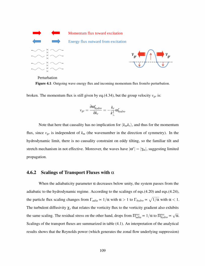
Energy flux outward from excitation
Perturbation
Momentum flux toward excitation
Figure 4.1: Outgoing wave energy flux and incoming momentum flux from/to perturbation.
broken. The momentum flux is still given by eq.(4.34), but the group velocity vgr is:
vgr =∂ωr
hydro
∂kr=− kr
k2⊥
ωrhydro
Note that here that causality has no implication for 〈kmkr〉, and thus for the momentum
flux, since vgr is independent of km (the wavenumber in the direction of symmetry). In the
hydrodynamic limit, there is no causality constraint on eddy tilting, so the familiar tilt and
stretch mechanism in not effective. Moreover, the waves have |ωr|= |γm|, suggesting limited
propagation.
4.6.2 Scalings of Transport Fluxes with α
When the adiabaticity parameter α decreases below unity, the system passes from the
adiabatic to the hydrodynamic regime. According to the scalings of eqs.(4.20) and eqs.(4.24),
the particle flux scaling changes from Γadia ∝ 1/α with α > 1 to Γhydro ∝√
1/α with α < 1.
The turbulent diffusivity χy that relates the vorticity flux to the vorticity gradient also exhibits
the same scaling. The residual stress on the other hand, drops from Πresadia ∝ 1/α to Πres
hydro ∝√
α.
Scalings of the transport fluxes are summarized in table (4.1). An interpretation of the analytical
results shows that the Reynolds power (which generates the zonal flow underlying suppression)
109
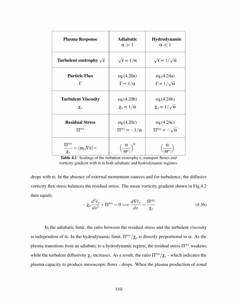
Plasma Response Adiabatic Hydrodynamicα 1 α 1
Turbulent enstrophy√
ε√
ε ∝ 1/α√
ε ∝ 1/√
α
Particle Flux eq.(4.20a) eq.(4.24a)
Γ Γ ∝ 1/α Γ ∝ 1/√
α
Turbulent Viscosity eq.(4.20b) eq.(4.24b)
χy χy ∝ 1/α χy ∝ 1/√
α
Residual Stress eq.(4.20c) eq.(4.24c)
Πres Πres ∝−1/α Πres ∝−√
α
Πres
χy= (ωci∇n)×
(α
|ω?|
)0 (α
|ω?|
)Table 4.1: Scalings of the turbulent enstrophy ε, transport fluxes and
vorticity gradient with α in both adiabatic and hydrodynamic regimes.
drops with α. In the absence of external momentum sources and for turbulence, the diffusive
vorticity flux stress balances the residual stress. The mean vorticity gradient shown in Fig.4.2
then equals:
−χyd2vy
dx2 +Πres = 0 =⇒
d∇vy
dx=
Πres
χy(4.36)
In the adiabatic limit, the ratio between the residual stress and the turbulent viscosity
is independent of α. In the hydrodynamic limit, Πres/χy is directly proportional to α. As the
plasma transitions from an adiabatic to a hydrodynamic regime, the residual stress Πres weakens,
while the turbulent diffusivity χy increases. As a result, the ratio Πres/χy - which indicates the
plasma capacity to produce mesoscopic flows - drops. When the plasma production of zonal
110
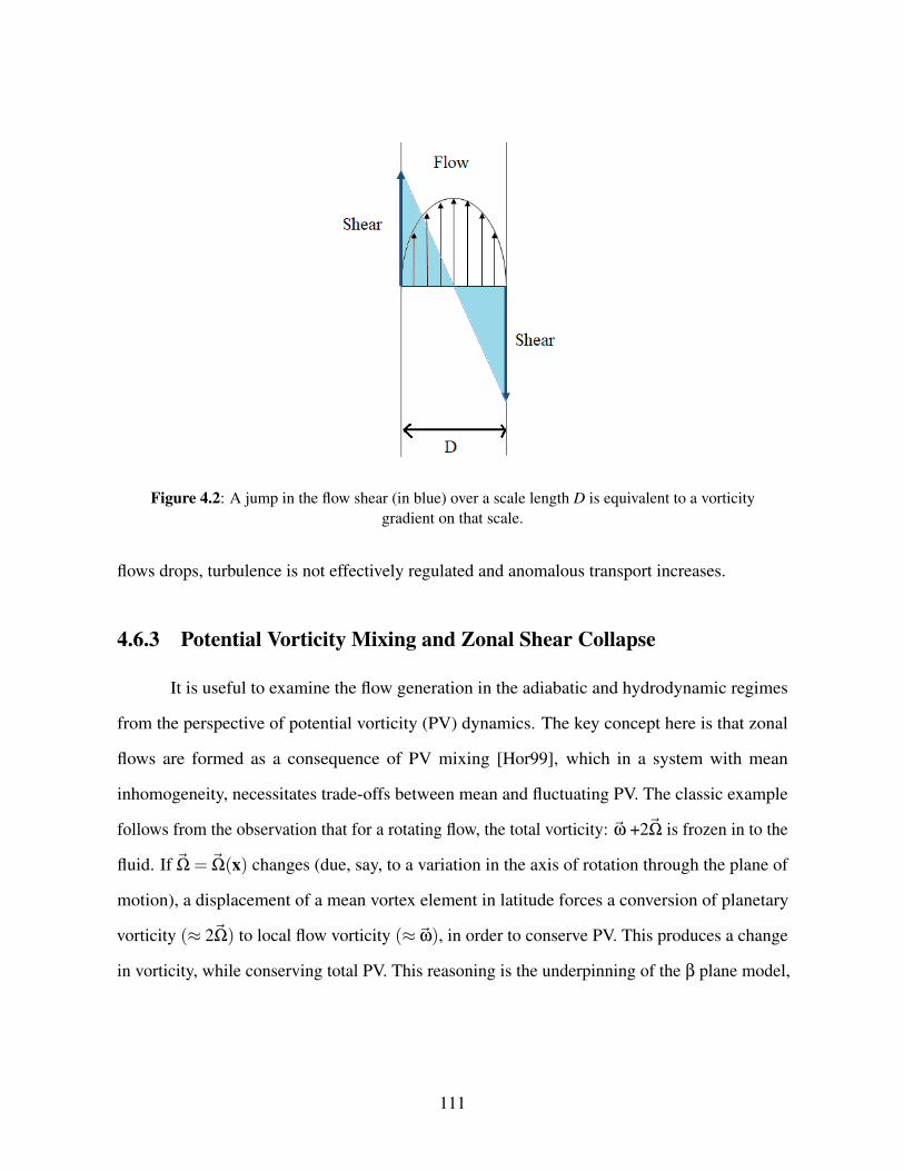
Figure 4.2: A jump in the flow shear (in blue) over a scale length D is equivalent to a vorticitygradient on that scale.
flows drops, turbulence is not effectively regulated and anomalous transport increases.
4.6.3 Potential Vorticity Mixing and Zonal Shear Collapse
It is useful to examine the flow generation in the adiabatic and hydrodynamic regimes
from the perspective of potential vorticity (PV) dynamics. The key concept here is that zonal
flows are formed as a consequence of PV mixing [Hor99], which in a system with mean
inhomogeneity, necessitates trade-offs between mean and fluctuating PV. The classic example
follows from the observation that for a rotating flow, the total vorticity: ~ω +2~Ω is frozen in to the
fluid. If ~Ω = ~Ω(x) changes (due, say, to a variation in the axis of rotation through the plane of
motion), a displacement of a mean vortex element in latitude forces a conversion of planetary
vorticity (≈ 2~Ω) to local flow vorticity (≈~ω), in order to conserve PV. This produces a change
in vorticity, while conserving total PV. This reasoning is the underpinning of the β plane model,
111
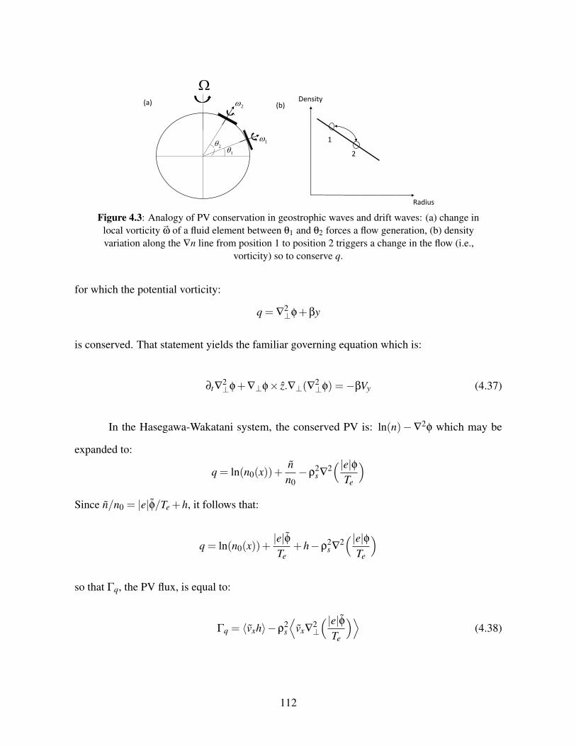
12
1
2Density
Radius
1
2
(a) (b)
Figure 4.3: Analogy of PV conservation in geostrophic waves and drift waves: (a) change inlocal vorticity ~ω of a fluid element between θ1 and θ2 forces a flow generation, (b) densityvariation along the ∇n line from position 1 to position 2 triggers a change in the flow (i.e.,
vorticity) so to conserve q.
for which the potential vorticity:
q = ∇2⊥φ+βy
is conserved. That statement yields the familiar governing equation which is:
∂t∇2⊥φ+∇⊥φ× z.∇⊥(∇2
⊥φ) =−βVy (4.37)
In the Hasegawa-Wakatani system, the conserved PV is: ln(n)−∇2φ which may be
expanded to:
q = ln(n0(x))+nn0−ρ
2s ∇
2( |e|φ
Te
)Since n/n0 = |e|φ/Te +h, it follows that:
q = ln(n0(x))+|e|φTe
+h−ρ2s ∇
2( |e|φ
Te
)
so that Γq, the PV flux, is equal to:
Γq = 〈vxh〉−ρ2s
⟨vx∇
2⊥
( |e|φTe
)⟩(4.38)
112
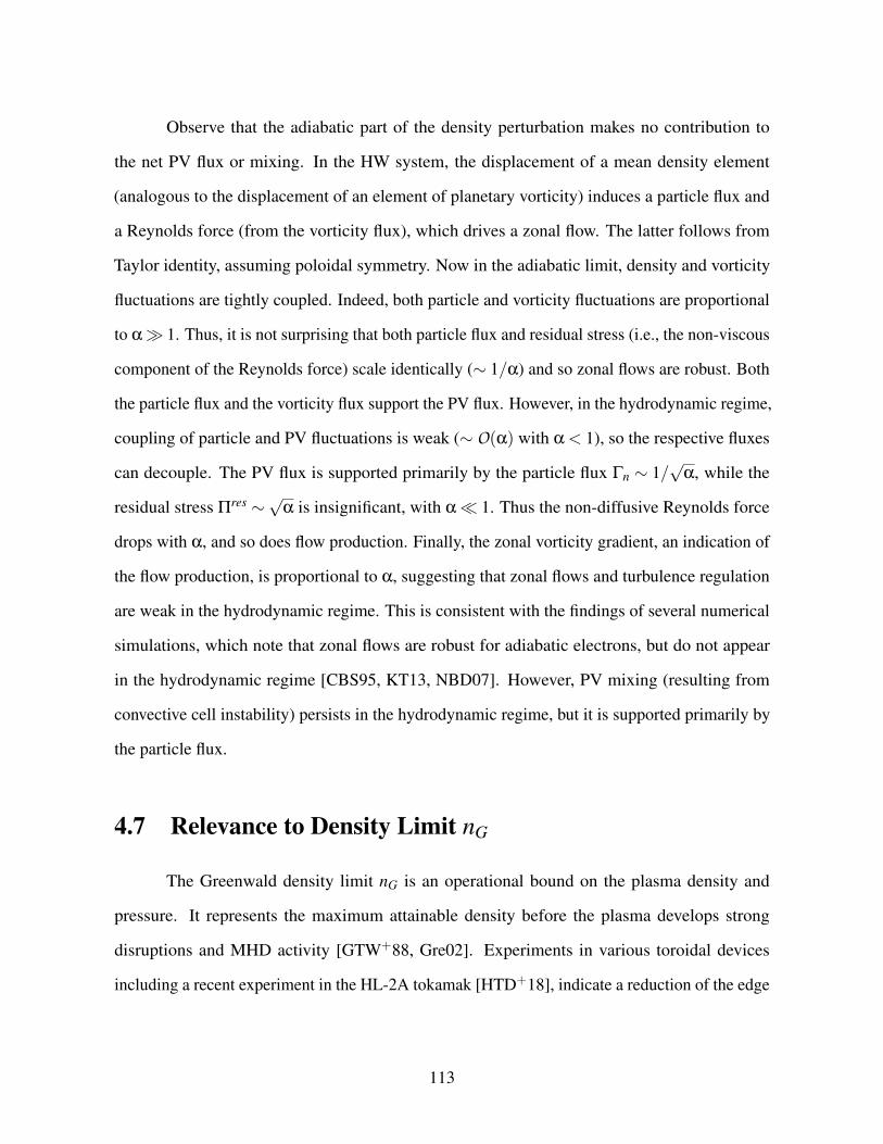
Observe that the adiabatic part of the density perturbation makes no contribution to
the net PV flux or mixing. In the HW system, the displacement of a mean density element
(analogous to the displacement of an element of planetary vorticity) induces a particle flux and
a Reynolds force (from the vorticity flux), which drives a zonal flow. The latter follows from
Taylor identity, assuming poloidal symmetry. Now in the adiabatic limit, density and vorticity
fluctuations are tightly coupled. Indeed, both particle and vorticity fluctuations are proportional
to α 1. Thus, it is not surprising that both particle flux and residual stress (i.e., the non-viscous
component of the Reynolds force) scale identically (∼ 1/α) and so zonal flows are robust. Both
the particle flux and the vorticity flux support the PV flux. However, in the hydrodynamic regime,
coupling of particle and PV fluctuations is weak (∼ O(α) with α < 1), so the respective fluxes
can decouple. The PV flux is supported primarily by the particle flux Γn ∼ 1/√
α, while the
residual stress Πres ∼√
α is insignificant, with α 1. Thus the non-diffusive Reynolds force
drops with α, and so does flow production. Finally, the zonal vorticity gradient, an indication of
the flow production, is proportional to α, suggesting that zonal flows and turbulence regulation
are weak in the hydrodynamic regime. This is consistent with the findings of several numerical
simulations, which note that zonal flows are robust for adiabatic electrons, but do not appear
in the hydrodynamic regime [CBS95, KT13, NBD07]. However, PV mixing (resulting from
convective cell instability) persists in the hydrodynamic regime, but it is supported primarily by
the particle flux.
4.7 Relevance to Density Limit nG
The Greenwald density limit nG is an operational bound on the plasma density and
pressure. It represents the maximum attainable density before the plasma develops strong
disruptions and MHD activity [GTW+88, Gre02]. Experiments in various toroidal devices
including a recent experiment in the HL-2A tokamak [HTD+18], indicate a reduction of the edge
113
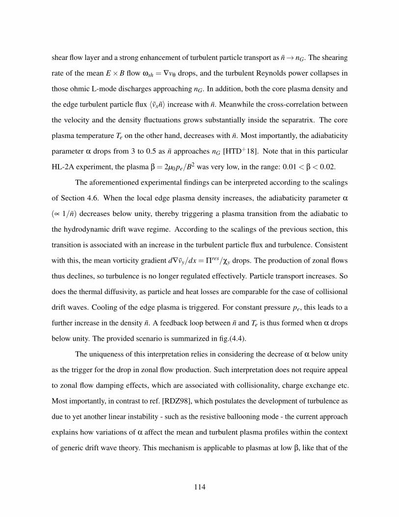
shear flow layer and a strong enhancement of turbulent particle transport as n→ nG. The shearing
rate of the mean E×B flow ωsh = ∇vθ drops, and the turbulent Reynolds power collapses in
those ohmic L-mode discharges approaching nG. In addition, both the core plasma density and
the edge turbulent particle flux 〈vxn〉 increase with n. Meanwhile the cross-correlation between
the velocity and the density fluctuations grows substantially inside the separatrix. The core
plasma temperature Te on the other hand, decreases with n. Most importantly, the adiabaticity
parameter α drops from 3 to 0.5 as n approaches nG [HTD+18]. Note that in this particular
HL-2A experiment, the plasma β = 2µ0 pe/B2 was very low, in the range: 0.01 < β < 0.02.
The aforementioned experimental findings can be interpreted according to the scalings
of Section 4.6. When the local edge plasma density increases, the adiabaticity parameter α
(∝ 1/n) decreases below unity, thereby triggering a plasma transition from the adiabatic to
the hydrodynamic drift wave regime. According to the scalings of the previous section, this
transition is associated with an increase in the turbulent particle flux and turbulence. Consistent
with this, the mean vorticity gradient d∇vy/dx = Πres/χy drops. The production of zonal flows
thus declines, so turbulence is no longer regulated effectively. Particle transport increases. So
does the thermal diffusivity, as particle and heat losses are comparable for the case of collisional
drift waves. Cooling of the edge plasma is triggered. For constant pressure pe, this leads to a
further increase in the density n. A feedback loop between n and Te is thus formed when α drops
below unity. The provided scenario is summarized in fig.(4.4).
The uniqueness of this interpretation relies in considering the decrease of α below unity
as the trigger for the drop in zonal flow production. Such interpretation does not require appeal
to zonal flow damping effects, which are associated with collisionality, charge exchange etc.
Most importantly, in contrast to ref. [RDZ98], which postulates the development of turbulence as
due to yet another linear instability - such as the resistive ballooning mode - the current approach
explains how variations of α affect the mean and turbulent plasma profiles within the context
of generic drift wave theory. This mechanism is applicable to plasmas at low β, like that of the
114
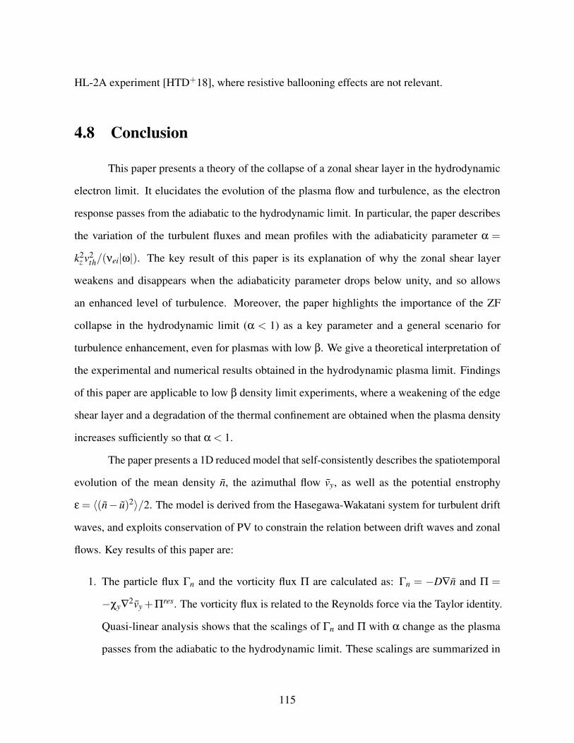
HL-2A experiment [HTD+18], where resistive ballooning effects are not relevant.
4.8 Conclusion
This paper presents a theory of the collapse of a zonal shear layer in the hydrodynamic
electron limit. It elucidates the evolution of the plasma flow and turbulence, as the electron
response passes from the adiabatic to the hydrodynamic limit. In particular, the paper describes
the variation of the turbulent fluxes and mean profiles with the adiabaticity parameter α =
k2z v2
th/(νei|ω|). The key result of this paper is its explanation of why the zonal shear layer
weakens and disappears when the adiabaticity parameter drops below unity, and so allows
an enhanced level of turbulence. Moreover, the paper highlights the importance of the ZF
collapse in the hydrodynamic limit (α < 1) as a key parameter and a general scenario for
turbulence enhancement, even for plasmas with low β. We give a theoretical interpretation of
the experimental and numerical results obtained in the hydrodynamic plasma limit. Findings
of this paper are applicable to low β density limit experiments, where a weakening of the edge
shear layer and a degradation of the thermal confinement are obtained when the plasma density
increases sufficiently so that α < 1.
The paper presents a 1D reduced model that self-consistently describes the spatiotemporal
evolution of the mean density n, the azimuthal flow vy, as well as the potential enstrophy
ε = 〈(n− u)2〉/2. The model is derived from the Hasegawa-Wakatani system for turbulent drift
waves, and exploits conservation of PV to constrain the relation between drift waves and zonal
flows. Key results of this paper are:
1. The particle flux Γn and the vorticity flux Π are calculated as: Γn = −D∇n and Π =
−χy∇2vy +Πres. The vorticity flux is related to the Reynolds force via the Taylor identity.
Quasi-linear analysis shows that the scalings of Γn and Π with α change as the plasma
passes from the adiabatic to the hydrodynamic limit. These scalings are summarized in
115
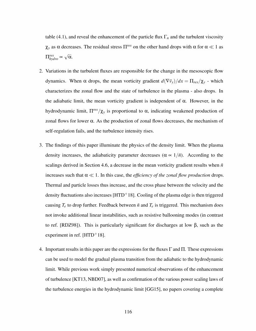
table (4.1), and reveal the enhancement of the particle flux Γn and the turbulent viscosity
χy as α decreases. The residual stress Πres on the other hand drops with α for α 1 as
Πreshydro ∝
√α.
2. Variations in the turbulent fluxes are responsible for the change in the mesoscopic flow
dynamics. When α drops, the mean vorticity gradient d(∇vy)/dx = Πres/χy - which
characterizes the zonal flow and the state of turbulence in the plasma - also drops. In
the adiabatic limit, the mean vorticity gradient is independent of α. However, in the
hydrodynamic limit, Πres/χy is proportional to α, indicating weakened production of
zonal flows for lower α. As the production of zonal flows decreases, the mechanism of
self-regulation fails, and the turbulence intensity rises.
3. The findings of this paper illuminate the physics of the density limit. When the plasma
density increases, the adiabaticity parameter decreases (α ∝ 1/n). According to the
scalings derived in Section 4.6, a decrease in the mean vorticity gradient results when n
increases such that α 1. In this case, the efficiency of the zonal flow production drops.
Thermal and particle losses thus increase, and the cross phase between the velocity and the
density fluctuations also increases [HTD+18]. Cooling of the plasma edge is then triggered
causing Te to drop further. Feedback between n and Te is triggered. This mechanism does
not invoke additional linear instabilities, such as resistive ballooning modes (in contrast
to ref. [RDZ98]). This is particularly significant for discharges at low β, such as the
experiment in ref. [HTD+18].
4. Important results in this paper are the expressions for the fluxes Γ and Π. These expressions
can be used to model the gradual plasma transition from the adiabatic to the hydrodynamic
limit. While previous work simply presented numerical observations of the enhancement
of turbulence [KT13, NBD07], as well as confirmation of the various power scaling laws of
the turbulence energies in the hydrodynamic limit [GG15], no papers covering a complete
116
transition from one limit to the other are presented. The underlying physics was not
explained.
5. The paper gives a simple physical picture of why ZF production drops in the hydrodynamic
electron regime. There the dispersion relation is ωhydror =
√ω?α/(2k2
⊥ρ2s ), so vgr =
−krωrhydro/k2
⊥. These are in contrast to the adiabatic case, for which ωadiar = ω?(1+
k2⊥ρ2
s )−1 and vgr = −2ρ2
s krkmvd/(1+ k2⊥ρ2
s )2. Thus, in the hydrodynamic regime, the
condition of outgoing waves (vgr > 0) does not constrain the Reynolds stress 〈vxvy〉 '
〈krkm〉, thus breaking the link between wave propagation and Reynolds stress. This link is
fundamental to ZF production by DWs.
6. The paper explains why turbulence is enhanced in the hydrodynamic limit, and ascertains
the physics of the Reynolds stress in regulating the drift wave - zonal flow relation. We
show that PV mixing in the hydrodynamic electron limit is supported by the particle flux,
i.e., 〈vxq〉= 〈vxh〉−〈vx∇2φ〉 ' 〈vxh〉. The vorticity flux drops and the particle flux rises
with α in this regime. This explains why zonal flow formation is weak in the hydrodynamic
regime.
Future work includes numerical investigation of the slow evolution of a plasma transition
from one limit to the other. Moreover, it would be instructive to investigate experimentally
the causality relation between the drop in α and the drop in ZF production. In particular, it
is useful to determine what occurs first. This would probe the predictions of the theory. One
suggestion would be to verify the decrease of the calculated total Reynolds work, as n/nG is
raised. When the total Reynolds work decreases, energy transfer to the mean flow structures
drops, so the fluctuations should grow. Another possible experiment consists of increasing the
plasma density n and temperature Te, such that the adiabaticity parameter α ∝ T 5/2e /n remains
constant (assuming the variations of the Coulomb logarithm are negligible). According to the
theory presented above, no collapse of the zonal shear layer should be observed, simply because
117
α does not change. One can also investigate the contribution of collisional damping effects
by comparing the response with and without the damping factor. This is particularly useful to
confirm the pivotal role of the Reynolds stress in the collapse of the zonal shear layer at the
density limit. Additional work also should include investigation of the role of high edge ∇p and
high β values in H-modes on the enhancement of turbulence and profile evolution in density
limit experiments.
4.9 Acknowledgments
The text and data in chapter 4 is a reprint of the material as currently being prepared for
submission for publication in Zonal Shear Layer Collapse in the Hydrodynamic Electron Limit
in the Journal of Physics of Plasmas 2018. Hajjar R. J., Diamond P. H., Malkov M., American
Institute of Physics, 2018. The dissertation author was the primary investigator and author of
this paper.
118
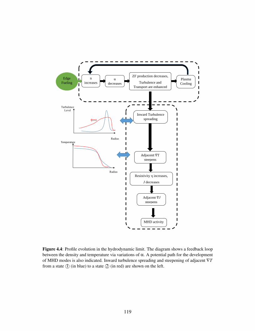
α
decreases
ZF production decreases,
Turbulence and
Transport are enhanced
Plasma
Cooling
Edge
Fueling
Inward Turbulence
spreading
Adjacent ∇T
steepens
Resistivity η increases,
J decreases
Adjacent ∇J
steepens
n
increases
MHD activity
Radius
Turbulence
Level
Radius
Temperature
Figure 4.4: Profile evolution in the hydrodynamic limit. The diagram shows a feedback loopbetween the density and temperature via variations of α. A potential path for the developmentof MHD modes is also indicated. Inward turbulence spreading and steepening of adjacent ∇Tfrom a state 1© (in blue) to a state 2© (in red) are shown on the left.
119
Chapter 5
SUMMARY AND FUTURE
DIRECTIONS
In this dissertation, the relationship between the microscopic drift wave turbulence and the
macroscopic zonal (perpendicular) and axial (parallel) flows was investigated. The dissertation
included a presentation of two analytical reduced models, as well as some simulation results
that validate and verify the previously published experimental data obtained from CSDX linear
plasma. In addition, one of these models explains the collapse of the zonal shear layer in the
plasma hydrodynamic electron limit closely related to the density limit experiments performed
on HL-2A tokamak. The models formulated in this dissertation are 1D (in radius) reduced
models that describe the physics of a multi-scale plasma. Such models are appropriate and
essential to understand the physics behind the feedback loops that exist between the microscopic
level and the macroscopic level in a multi-scale plasma. Moreover, reduced models generally
provide a better and more elaborate physical interpretation of the experimental results than
Direct Numerical Simulations (DNS), which have a high computational cost, and often fail
to provide a detailed insight into the actual physics of the plasma. Most importantly, reduced
models such as the ones presented in this dissertation can be easily coupled to other models
120
in the framework of future Plasma Material Interaction (PMI) studies. Such models provide a
useful new intermediate approach for the simulation of self-consistent evolution edge and SOL
plasma profiles, transverse and parallel flows and turbulence, and would allow the study of main
plasma and impurity dynamics across timescales ranging from a few turbulent correlation times
up to system equilibrium timescales. When modified to include toroidal and open-field line
effects, and extended to a 2D geometry along the magnetic field and binormal directions, the
proposed models bridge the gap between the existing time averaged fluid codes of the edge and
SOL region of confinement device, and fully turbulent direct numerical simulations. Here DNS
self-consistently capture the evolution of the plasma profile and its flow, but are computationally
expensive to use for long time scales. Such a new capability might be useful to study the
entrainment and transport of eroded wall impurities in flowing edge and SOL plasma, and the
long-time migration of these materials in the SOL and divertor regions of confinement devices.
This dissertation sought to investigate three topics:
1. How are axial flows generated in CSDX plasma, and is there a direct relation between the
axial and the perpendicular flow dynamics in the adiabatic plasma of CSDX? Moreover,
what is the analytical framework that describes the energy transfer between the flows and
turbulence in CSDX? (Chapter 2)
2. What is the appropriate analytical model that describes the turbulent potential energy
exchange between drift wave turbulence and zonal flows in CSDX plasma? (Chapter 3)
3. How is the predator/prey relation between drift waves and zonal flows previously discussed
in Chapter 2 and 3 affected in the hydrodynamic electron limit? (Chapter 4)
The conclusions reached after investigating each topic are presented at the end of each chapter.
In summary, the dissertation presents a comprehensive description of the theory behind the drift
wave turbulence and both zonal and axial flows. The presented numerical results highlight the
crucial role the Reynolds stresses play in regulating turbulence. Not only does this dissertation
121
formulate appropriate reduced models that describe the interactions between the mean profiles
and the fluctuations in the adiabatic electron limit, but also extends this description to the
hydrodynamic electron limit. The latter describes the behavior and dynamics of a plasma
characterized by a high density and low temperature. The constants introduced in Chapter 2
(σV T ) and Chapter 3 (RDT ) are novel criteria that describe parallel to perpendicular flow coupling,
as well as suppression of drift wave turbulence by the zonal flows.
In addition to what was presented in this dissertation, recommended future work includes:
1. Performing numerical simulations of the comprehensive model presented in Chapter 2,
and analyzing the numerical data in order to pinpoint the parallel to perpendicular flow
coupling in CSDX. It is thus recommended to calculate a numerical value for the coupling
constant σV T from the simulation profiles, and compare it to the value recovered from the
experimental data. In addition, it is also useful to perform numerical studies for the slaved
2-field model also presented in Chapter 2.
2. Adding an axial momentum source to the model of Chapter 2, in an attempt to mimic the
torque exerted on the plasma in toroidal devices. Adding an axial momentum source to the
model could be used to compare the relative magnitude of the intrinsic parallel flows to
the externally imposed ones. This is particularly helpful for studying the scaling of the
parallel intrinsic flow with the plasma characteristics in future plasma devices.
3. Simulating a full and complete plasma transition from the adiabatic to the hydrodynamic
limit. Such step is essential to characterize the changes in the mean and turbulent profiles
of the plasma. The numerical results should be ultimately compared to the experimental
data retrieved from various toroidal devices.
4. A study of the evolution of the plasma temperature, in addition to the variations in density
and flow as presented in Chapter 4. Accounting for temperature variations aims at exploring
the predator/prey relation in H-mode hydrodynamic limit plasmas.
122
5. Accounting for the effects of both charge-exchange reactions, as well as the ion-neutral
collisions in a hydrodynamic plasma. This step aims at studying the importance of
collisional zonal flow damping from a numerical perspective.
123
Bibliography
[AD16] A. Ashourvan and P. H. Diamond. How mesoscopic staircases condense tomacroscopic barriers in confined plasma turbulence. Phys. Rev. E, 94:051202,2016.
[ADG16] A. Ashourvan, P. H. Diamond, and O. D. Gurcan. Transport matrix for particlesand momentum in collisional drift waves turbulence in linear plasma devices.Physics of Plasmas, 23(2), 2016.
[AKI+09] H. Arakawa, K. Kamataki, S. Inagaki, T. Maruta, Y. Nagashima, T. Yamada,S. Shinohara, K. Terasaka, S. Sugita, M. Yagi, Nl Kasuya, Al Fujisawa, S-I.Itoh, and K. Itoh. Observations of abrupt changes in the fluctuation spectrum onLMD-U. Plasma Physics and Controlled Fusion, 51(8):085001, 2009.
[AYT07] G. Y. Antar, J. H. Yu, and G. Tynan. The origin of convective structures in thescrape-off layer of linear magnetic fusion devices investigated by fast imaging.Physics of Plasmas, 14(2), 2007.
[BDT90] H. Biglari, P. H. Diamond, and P. W. Terry. Influence of sheared poloidal rotationon edge turbulence. Physics of Fluids B: Plasma Physics, 2(1):1–4, 1990.
[BLSY98] N. J. Balmforth, S. G. Llewellyn Smith, and W. R. Young. Dynamics of interfacesand layers in a stratified turbulent fluid. Journal of Fluid Mechanics, 355:329–358,1 1998.
[BMT12] L. Biferale, S. Musacchio, and F. Toschi. Inverse energy cascade in three-dimensional isotropic turbulence. Phys. Rev. Lett., 108:164501, Apr 2012.
[BTA+05] M. J. Burin, G. R. Tynan, G. Y. Antar, N. A. Crocker, and C. Holland. On thetransition to drift turbulence in a magnetized plasma column. Physics of Plasmas,12(5), 2005.
[CAT+16] L. Cui, A. Ashourvan, S. C. Thakur, R. Hong, P. H. Diamond, and G. R. Ty-nan. Spontaneous profile self-organization in a simple realization of drift-waveturbulence. Physics of Plasmas, 23(5), 2016.
124
[CBS95] S. J. Camargo, D. Biskamp, and B. D. Scott. Resistive drift-wave turbulence.Physics of Plasmas, 2(1):48–62, 1995.
[Che84] F. F. Chen. Plasma Physics and Controlled Fusion. Plenum Press, New York,1984.
[CLGD93] B. A. Carreras, V. E. Lynch, L. Garcia, and P. H. Diamond. Resistive pressuregradient driven turbulence with self consistent flow profile evolution. Physics ofFluids B, 5(5):1491–1505, 1993.
[CTD+15] L. Cui, G. R. Tynan, P. H. Diamond, S. C. Thakur, and C. Brandt. Up-gradientparticle flux in a drift wave-zonal flow system. Physics of Plasmas, 22(5), 2015.
[DGH+08] P. H. Diamond, O. D. Gurcan, T. S. Hahm, K. Miki, Y. Kosuga, and X. Garbet.Momentum theorems and the structure of atmospheric jets and zonal flows inplasmas. Plasma Physics and Controlled Fusion, 50(12):124018, 2008.
[DIIH05] P. H. Diamond, S. I. Itoh, K. Itoh, and T. S. Hahm. Zonal flows in plasma; areview. Plasma Physics and Controlled Fusion, 47(5):R35–R161, 2005.
[DKG+13] P.H. Diamond, Y. Kosuga, .D. Grcan, C.J. McDevitt, T.S. Hahm, N. Fedorczak,J.E. Rice, W.X. Wang, S. Ku, J.M. Kwon, G. Dif-Pradalier, J. Abiteboul, L. Wang,W.H. Ko, Y.J. Shi, K. Ida, W. Solomon, H. Jhang, S.S. Kim, S. Yi, S.H. Ko,Y. Sarazin, R. Singh, and C.S. Chang. An overview of intrinsic torque and momen-tum transport bifurcations in toroidal plasmas. Nuclear Fusion, 53(10):104019,2013.
[DLCT94] P. H. Diamond, Y.-M. Liang, B. A. Carreras, and P. W. Terry. Self-regulatingshear flow turbulence: A paradigm for the l to h transition. Phys. Rev. Lett.,72:2565–2568, Apr 1994.
[DMG+09] P. H. Diamond, C.J. McDevitt, .D. Grcan, T.S. Hahm, W. X. Wang, E.S. Yoon,I. Holod, Z. Lin, V. Naulin, and R. Singh. Physics of non-diffusive turbulenttransport of momentum and the origins of spontaneous rotation in tokamaks.Nuclear Fusion, 49(4):045002, 2009.
[EHH+10] T. Estrada, T. Happel, C. Hidalgo, E. Ascasbar, and E. Blanco. Experimen-tal observation of coupling between turbulence and sheared flows during L-Htransitions in a toroidal plasma. EPL (Europhysics Letters), 92(3):35001, 2010.
[FII+04] A. Fujisawa, K. Itoh, H. Iguchi, K. Matsuoka, S. Okamura, A. Shimizu, T. Minami,Y. Yoshimura, K. Nagaoka, C. Takahashi, M. Kojima, H. Nakano, S. Ohsima,S. Nishimura, M. Isobe, C. Suzuki, T Akiyama, K. Ida, K. Toi, S.-I. Itoh, andP. H. Diamond. Identification of zonal flows in a toroidal plasma. Phys. Rev.Lett., 93:165002, Oct 2004.
125
[Gar01] X. Garbet. Turbulence in fusion plasmas: key issues and impact on transportmodelling. Plasma Physics and Controlled Fusion, 43(12A):A251, 2001.
[GDH06] O. D. Grcan, P. H. Diamond, and T. S. Hahm. Radial transport of fluctua-tion energy in a two-field model of drift-wave turbulence. Physics of Plasmas,13(5):052306, 2006.
[GDH07] O. D. Gurcan, P. H. Diamond, and T. S. Hahm. Spatial and spectral evolution ofturbulence. Physics of Plasmas, 14(5), 2007.
[GDH08] O. D. Gurcan, P. H. Diamond, and T. S. Hahm. Turbulent equipartition andhomogenization of plasma angular momentum. Phys. Rev. Lett., 100:135001,Apr 2008.
[GDHS07] O. D. Gurcan, P. H. Diamond, T. S. Hahm, and R. Singh. Intrinsic rotation andelectric field shear. Physics of Plasmas, 14(4):042306, 2007.
[GG15] K. Ghantous and O. D. Gurcan. Wave-number spectrum of dissipative drift wavesand a transition scale. Phys. Rev. E, 92:033107, 2015.
[GKP+03] P. Gohil, J. Kinsey, V. Parail, X. Litaudon, T. Fukuda, T. Hoang, for the ITPAGroup on Transport, ITB Physics: J. Connor, E.J. Doyle, Yu. Esipchuk, T. Fujita,T. Fukuda, P. Gohil, J. Kinsey, S. Lebedev, X. Litaudon, V. Mukhovatov, J. Rice,E. Synakowski, K. Toi, B. Unterberg, V. Vershkov, M. Wakatani, J. Weiland,for the International ITB Database Working Group: T. Aniel, Yu.F. Baranov,E. Barbato, A. Bcoulet, C. Bourdelle, G. Bracco, R.V. Budny, P. Buratti, E.J.Doyle, L. Ericsson, Yu. Esipchuk, B. Esposito, T. Fujita, T. Fukuda, P. Gohil,C. Greenfield, M. Greenwald, T. Hahm, T. Hellsten, T. Hoang, D. Hogeweij,S. Ide, F. Imbeaux, Y. Kamada, J. Kinsey, N. Kirneva, X. Litaudon, P. Maget,A. Peeters, K. Razumova, F. Ryter, Y. Sakamoto, H. Shirai, G. Sips, T. Suzuki,E. Synakowski, and T.Takizuka. Increased understanding of the dynamics andtransport in itb plasmas from multi-machine comparisons. Nuclear Fusion,43(8):708, 2003.
[GmcHP+06] B. Goncalves, C. Hidalgo, M. A. Pedrosa, R. O. Orozco, E. Sanchez, and C. Silva.Role of turbulence on edge momentum redistribution in the tj-ii stellarator. Phys.Rev. Lett., 96:145001, Apr 2006.
[Gre02] M. Greenwald. Density limits in toroidal plasmas. Plasma Phys. Control. Fusion,44:R27, 2002.
[GTA+99] A. M. Garofalo, A. D. Turnbull, M. E. Austin, J. Bialek, M. S. Chu, K. J. Comer,E. D. Fredrickson, R. J. Groebner, R. J. La Haye, L. L. Lao, E. A. Lazarus, G. A.Navratil, T. H. Osborne, B. W. Rice, S. A. Sabbagh, J. T. Scoville, E. J. Strait,and T. S. Taylor. Direct observation of the resistive wall mode in a tokamak andits interaction with plasma rotation. Phys. Rev. Lett., 82:3811–3814, May 1999.
126
[GTW+88] M. Greenwald, J. L. Terry, S. M. Wolfe1, S. Ejima, M. G. Bell, S. M. Kaye, andG.H. Neilson. Nuclear Fusion, 28:2199, 1988.
[HB95] T. S. Hahm and K. H. Burrell. Flow shear induced fluctuation suppression infinite aspect ratio shaped tokamak plasma. Physics of Plasmas, 2(5):1648–1651,1995.
[HDAT17] R. J. Hajjar, P. H. Diamond, A. Ashourvan, and G. R. Tynan. Modelling enhancedconfinement in drift-wave turbulence. Physics of Plasmas, 24(6):062106, 2017.
[Hin91] F. L. Hinton. Thermal confinement bifurcation and the L to H mode transition intokamaks. Physics of Fluids B, 3(3):696–704, 1991.
[HLH+17] R. Hong, J. C. Li, R. J. Hajjar, S. Thakur, P. H. Diamond, and G. R. Tynan.Generation of parasitic axial flow by drift wave turbulence with broken symmetry:Theory and experiment. submitted to Physics of Plasmas, 2017.
[HLT+17] R. Hong, J. C. Li, S. Thakur, R. J. Hajjar, P. H. Diamond, and G. R. Tynan.Tracing the pathway from drift-wave turbulence with broken symmetry to theproduction of sheared axial mean flow. submitted to Physical Review Letters,2017.
[HM77] A. Hasegawa and K. Mima. Stationary spectrum of strong turbulence in magne-tized nonuniform plasma. Phys. Rev. Lett., 39:205–208, 1977.
[Hol16] C. Holland. Validation metrics for turbulent plasma transport. Physics of Plasmas,23(6), 2016.
[Hor99] W. Horton. Drift waves and transport. Rev. Mod. Phys., 71:735–778, 1999.
[HS93] F. L. Hinton and G. M. Staebler. Particle and energy confinement bifurcation intokamaks. Physics of Fluids B: Plasma Physics, 5(4):1281–1288, 1993.
[HTD+18] R. Hong, G.R. Tynan, P.H. Diamond, L. Nie, D. Guo, T. Long, R. Ke, Y. Wu,B. Yuan, M. Xu, and The HL-2A Team. Edge shear flows and particle transportnear the density limit of the HL-2A tokamak. Nuclear Fusion, 58(1):016041,2018.
[HW83] A. Hasegawa and M. Wakatani. Plasma edge turbulence. Phys. Rev. Lett., 50:682,1983.
[HW87] A. Hasegawa and M. Wakatani. Self-organization of electrostatic turbulence in acylindrical plasma. Phys. Rev. Lett., 59:1581–1584, Oct 1987.
[II96] K. Itoh and S.-I Itoh. Plasma Phys. Control. Fusion, 38:1, 1996.
[IIFY99] K. Itoh, S. I. Itoh, A. Fukuyama, and M. Yagi. Transport and structural formationin plasmas. IOP, 1999.
127
[IKI+16] S. Inagaki, T. Kobayashi, S. I. Itoh, T. Mitsuzono, H. Arakawa, T. Yamada,Y. Miwa, N. Kasuya, M. Sasaki, M Lesur, A. Fujisawa, and K. Itoh. A concept ofcross-ferroic plasma turbulence. Scientific Reports, 6(22189), 2016.
[ite] Iter official website. https://www.iter.org/. Accessed: 2018-02-10.
[KD03] E. J. Kim and P. H. Diamond. Zonal flows and transient dynamics of the L-Htransition. Phys. Rev. Lett., 90:185006, 2003.
[KDG10] Y. Kosuga, P. H. Diamond, and . D. Grcan. On the efficiency of intrinsic rotationgeneration in tokamaks. Physics of Plasmas, 17(10):102313, 2010.
[KII16] Y. Kosuga, S.-I. Itoh, and K. Itoh. Turbulence dynamics with the coupling ofdensity gradient and parallel velocity gradient in the edge plasmas. Contributionsto Plasma Physics, 56(6-8):511–515, 2016.
[KII17] Y. Kosuga, S.-I. Itoh, and K. Itoh. Zonal flow generation in parallel flow sheardriven turbulence. Physics of Plasmas, 24(3):032304, 2017.
[KIIe5] Y. Kosuga, S-I. Itoh, and K. Itoh. Density peaking by parallel flow shear driveninstability. Plasma and Fusion Research, 10:3401024–3401024, 201the5.
[KIK+16] T. Kobayashi, S. Inagaki, Y. Kosuga, M. Sasaki, Y. Nagashima, T. Yamada,H. Arakawa, N. Kasuya, A. Fujisawa, S.-I. Itoh, and K. Itoh. Structure formationin parallel ion flow and density profiles by cross-ferroic turbulent transport inlinear magnetized plasma. Physics of Plasmas, 23(10), 2016.
[KJD+11] S. S. Kim, H. Jhang, P. H. Diamond, L. Terzolo, S. Yi, and T.S. Hahm. Intrinsicrotation, hysteresis and back transition in reversed shear internal transport barriers.Nuclear Fusion, 51(7):073021, 2011.
[KLP+97] T. Klinger, A. Latten, A. Piel, G. Bonhomme, and T. Pierre. Chaos and turbulencestudies in low-β plasmas. Plasma Phys. Control. Fusion, 39:B145, 1997.
[KT13] J. Kim and P. W. Terry. Numerical investigation of frequency spectrum in theHasegawa-Wakatani model. Physics of Plasmas, 20(10):102303, 2013.
[LD17] J. C. Li and P. H. Diamond. Negative viscosity from negative compressibilityand axial flow shear stiffness in a straight magnetic field. Physics of Plasmas,24(3):032117, 2017.
[LDXT16] J. C. Li, P. H. Diamond, X. Q. Xu, and G. R. Tynan. Dynamics of intrinsic axialflows in unsheared, uniform magnetic fields. Physics of Plasmas, 23(5), 2016.
[LL94] M. A. Lieberman and A. J. Lichtenberg. Principles of Plasma Discharges andMaterials Processing. Wiley Interscience Publication, New York, 1994.
128
[MAP09] P. D. Mininni, A. Alexakis, and A. Pouquet. Scale interactions and scaling laws inrotating flows at moderate rossby numbers and large reynolds numbers. Physicsof Fluids, 21(1):015108, 2009.
[MBB+11] S. H. Muller, J. A. Boedo, K. H. Burrell, J. S. deGrassie, R. A. Moyer, D. L.Rudakov, W. M. Solomon, and G. R. Tynan. Intrinsic rotation generation inELM-free H-mode plasmas in the DIII-D tokamak - experimental observations.Physics of Plasmas, 18(7), 2011.
[MD10] K. Miki and P. H. Diamond. Role of the geodesic acoustic mode shearingfeedback loop in transport bifurcations and turbulence spreading. Physics ofPlasmas, 17(3):032309, 2010.
[MDG+12] K. Miki, P. H. Diamond, O. D. Gurcan, G. R. Tynan, T. Estrada, L. Schmitz, andG. S. Xu. Spatio-temporal evolution of the L-I-H transition. Physics of Plasmas,19(9), 2012.
[MDM+15] M. A. Malkov, P. H. Diamond, K. Miki, J. E. Rice, and G. R. Tynan. Linking themicro and macro: L - H transition dynamics and threshold physics. Physics ofPlasmas, 22(3), 2015.
[MRS09] P. Manz, M. Ramisch, and U. Stroth. Physical mechanism behind zonal-flowgeneration in drift-wave turbulence. Phys. Rev. Lett., 103:165004, 2009.
[MXTT11] P. Manz, M. Xu, S. C. Thakur, and G. R. Tynan. Nonlinear energy transfer duringthe transition to drift-interchange turbulence. Plasma Physics and ControlledFusion, 53(9):095001, 2011.
[NBD07] R. Numata, R. Ball, and R. L. Dewar. Bifurcation in electrostatic resistive driftwave turbulence. Physics of Plasmas, 14(10):102312, 2007.
[OT] W. L. Oberkampf and T. G. Trucano. Some specific features of atmosphericturbulence. Progress in Aerospace Sciences, 38(3):209–272.
[PBN13] A. V. Pushkarev, W. J. T. Bos, and S. V. Nazarenko. Zonal flow generation and itsfeedback on turbulence production in drift wave turbulence. Physics of Plasmas,20(4):042304, 2013.
[Pec13] H. Pecseli. Waves and Oscillations in PLasmas. CRC Press, Abingdon-U.K.,first edition edition, 2013.
[Pop08] S. Pope. Turbulent Flows. Cambridge University Press, Cambridge, UK, 2008.
[RDZ98] B. N. Rogers, J. F. Drake, and A. Zeiler. Phase space of tokamak edge turbulence,the L−H transition, and the formation of the edge pedestal. Phys. Rev. Lett.,81:4396–4399, 1998.
129
[RHD+11] J. E. Rice, J. W. Hughes, P. H. Diamond, Y. Kosuga, Y. A. Podpaly, M. L. Reinke,M. J. Greenwald, O. D. Gurcan, T. S. Hahm, A. E. Hubbard, E. S. Marmar, C. J.McDevitt, and D. G. Whyte. Edge temperature gradient as intrinsic rotation drivein alcator c-mod tokamak plasmas. Phys. Rev. Lett., 106:215001, May 2011.
[Rhi75] P. B. Rhines. Waves and turbulence on a beta-plane. Journal of Fluid Mechanics,69:417–443, 6 1975.
[RMRP92] T. D. Rognlien, J. L. Milovich, M. E. Rensink, and G. D. Porter. A fully implicit,time dependent 2-D fluid code for modeling tokamak edge plasmas. Journal ofNuclear Materials, 196-198(Supplement C):347 – 351, 1992. Plasma-SurfaceInteractions in Controlled Fusion Devices.
[Sco05] B. D. Scott. Energetics of the interaction between electromagnetic E × B turbu-lence and zonal flows. New Journal of Physics, 7(1):92, 2005.
[SDSK13] T. Stoltzfus-Dueck, B. D. Scott, and J. A. Krommes. Nonadiabatic electronresponse in the hasegawa-wakatani equations. Physics of Plasmas, 20(8):082314,2013.
[SGK+99] U. Stroth, T. Geist, J. P. T. Koponen, H.-J. Hartfuß, P. Zeiler, ECRH, and W7-ASteam. Evidence for convective inward particle transport in a stellarator. Phys.Rev. Lett., 82:928–931, Feb 1999.
[SM00] W. D. Smyth and J. N. Moum. Length scales of turbulence in stably stratifiedmixing layers. Physics of Fluids, 12(6):1327–1342, 2000.
[Sta05] W. M. Stacey. Fusion Plasma Physics. Wiley VCH, Weinheim, Germany, 2005.
[SZR+12] L. Schmitz, L. Zeng, T. L. Rhodes, J. C. Hillesheim, E. J. Doyle, R. J. Groebner,W. A. Peebles, K. H. Burrell, and G. Wang. Role of zonal flow predator-preyoscillations in triggering the transition to H-mode confinement. Phys. Rev. Lett.,108:155002, Apr 2012.
[Tay15] G. I. Taylor. Eddy motion in the atmosphere. Philosophical Transactions of theRoyal Society of London A: Mathematical, Physical and Engineering Sciences,215(523-537):1–26, 1915.
[TBC+14] S. C. Thakur, C Brandt, L. Cui, J. J. Gosselin, A. D. Light, and G. R. Tynan.Multi-instability plasma dynamics during the route to fully developed turbulencein a helicon plasma. Plasma Sources Science and Technology, 23(4):044006,2014.
[TBI+04] T. Tala, C. Bourdelle, F. Imbeaux, D. Moreau, V. Parail, G. Corrigan, F. Crisanti,X. Garbet, D. Heading., E. Joffrin, L. Laborde, X. Litaudon, P. et al Mantica, PrStrand, and Jan Weiland. Progress in transport modeling of internal transport
130
barrier plasmas in jet. In 20th IAEA Fusion Energy Conference, Villamoura,Portugal November 1-6, IAEA, pages Paper TH / P2–9, 2004.
[Ter00] P. W. Terry. Suppression of turbulence and transport by sheared flow. Rev. Mod.Phys., 72:109–165, 2000.
[TGM+16] S. C. Thakur, J. J. Gosselin, J. McKee, E. E. Scime, S. H. Sears, and G. R.Tynan. Development of core ion temperature gradients and edge sheared flows ina helicon plasma device investigated by laser induced fluorescence measurements.Physics of Plasmas, 23(8):082112, 2016.
[TGT+10] P. Tamain, Ph. Ghendrih, E. Tsitrone, V. Grandgirard, X. Garbet, Y. Sarazin,E. Serre, G. Ciraolo, and G. Chiavassa. Tokam-3d: A 3d fluid code for trans-port and turbulence in the edge plasma of tokamaks. Journal of ComputationalPhysics, 229(2):361 – 378, 2010.
[THY+06] G. R. Tynan, C. Holland, J. H. Yu, A. James, D. Nishijima, M. Shimada, andN. Taheri. Observation of turbulent-driven shear flow in a cylindrical laboratoryplasma device. Plasma Physics and Controlled Fusion, 48(4):S51, 2006.
[TKE+99] P. L. Taylor, A. G. Kellman, T. E. Evans, D. S. Gray, D. A. Humphreys, A. W.Hyatt, T. C. Jemigan, R. L. Lee, J. A. Leur, S. C. Luckhardt, P. B. Prks, M. J.Schaffer, D. G. Whyte, and J. Zhang. Disruption mitigation studies in diii-d.Physics of Plasma, 6:1872, 1999.
[TKL05] M. Z. Tokar, F. A. Kelly, and X. Loozen. Role of thermal instabilities andanomalous transport in threshold of detachment and multifacetted asymmetricradiation from the edge (MARFE). Physics of Plasmas, 12(5):052510, 2005.
[Tok03] M. Z. Tokar. Synergy of anomalous transport and radiation in the density limit.Phys. Rev. Lett., 91:095001, 2003.
[TXD+13] G. R. Tynan, M. Xu, P.H. Diamond, J.A. Boedo, I. Cziegler, N. Fedorczak,P. Manz, K. Miki, S. Thakur, L. Schmitz, L. Zeng, E.J. Doyle, G. M. McKee,Z. Yan, G. S. Xu, B. N. Wan, H. Q. Wang, H. Y. Guo, J. Dong, K. Zhao, J. Cheng,W. Y. Hong, and L. W. Yan. Turbulent-driven low-frequency sheared E×B flowsas the trigger for the h-mode transition. Nuclear Fusion, 53(7):073053, 2013.
[WDH12] L. Wang, P. H. Diamond, and T. S. Hahm. How does drift wave turbulence convertparallel compression into perpendicular flows? Plasma Physics and ControlledFusion, 54(9):095015, 2012.
[Wes04] J. Wesson. Tokamaks. Clarendon Press, Oxford,UK, third edition, 2004.
[WGE+17] W. X. Wang, B. A. Grierson, S. Ethier, J. Chen, E. Startsev, and P. H. Diamond.Understanding and predicting profile structure and parametric scaling of intrinsicrotation. Physics of Plasmas, 24(9):092501, 2017.
131
[WRK+15] S. Wiesen, D. Reiter, V. Kotov, M. Baelmans, W. Dekeyser, A.S. Kukushkin, S.W.Lisgo, R.A. Pitts, V. Rozhansky, G. Saibene, I. Veselova, and S. Voskoboynikov.The new solps-iter code package. Journal of Nuclear Materials, 463(SupplementC):480 – 484, 2015. PLASMA-SURFACE INTERACTIONS 21.
[XBFS11] H. Xia, D. Byrne, G. Falkovich, and M. Shats. Upscale energy transfer in thickturbulent fluid layers. Nature Physics, 7:321–324, 2011.
[XTD+12] M. Xu, G. R. Tynan, P. H. Diamond, P. Manz, C. Holland, N. Fedorczak,S. Chakraborty Thakur, J. H. Yu, K. J. Zhao, J. Q. Dong, J. Cheng, W. Y. Hong,L. W. Yan, Q. W. Yang, X. M. Song, Y. Huang, L. Z. Cai, W. L. Zhong, Z. B.Shi, X. T. Ding, X. R. Duan, and Y. Liu. Frequency-resolved nonlinear turbulentenergy transfer into zonal flows in strongly heated L-mode plasmas in the HL-2Atokamak. Phys. Rev. Lett., 108:245001, 2012.
[XTH+09] M. Xu, G. R. Tynan, C. Holland, Z. Yan, S. H. Muller, and J. H. Yu. Studyof nonlinear spectral energy transfer in frequency domain. Physics of Plasmas,16(4):042312, 2009.
[XWW+11] G. S. Xu, B. N. Wan, H. Q. Wang, H. Y. Guo, H. L. Zhao, A. D. Liu, V. Naulin,P. H. Diamond, G. R. Tynan, M. Xu, R. Chen, M. Jiang, P. Liu, N. Yan, W. Zhang,L. Wang, S. C. Liu, and S. Y. Ding. First evidence of the role of zonal flowsfor the L-H transition at marginal input power in the EAST tokamak. Phys. Rev.Lett., 107:125001, Sep 2011.
[YII03] A. Yoshizawa, S. Itoh, and K. Itoh. Plasma and Fluid Turbulence: Theory andModeling. Institute of Physics Publishing, London, 2003.
[YTH+10] Z. Yan, G. R. Tynan, C. Holland, M. Xu, S. H. Muller, and J. H. Yu. Scalingproperties of turbulence driven shear flow. Physics of Plasmas, 17(1):012302,2010.
[ZHB+10] S. Zhou, W. W. Heidbrink, H. Boehmer, R. McWilliams, T. Carter, S. Vincena,S. K. P. Tripathi, P. Popovich, B. Friedman, and F. Jenko. Turbulent transport offast ions in the large plasma device. Physics of Plasmas, 17(9), 2010.
[ZMH+10] S. J. Zweben, R. J. Maqueda, R. Hager, K. Hallatschek, S. M. Kaye, T. Munsat,F. M. Poli, A. L. Roquemore, Y. Sechrest, and D. P. Stotler. Quiet periods in edgeturbulence preceding the L-H transition in the national spherical torus experiment.Physics of Plasmas, 17(10), 2010.
132


