Ecology Letters, (2005) 8: 224–239 doi: 10.1111/j.1461...

REV I EWThe role of spatial scale and the perception

of large-scale species-richness patterns

Carsten Rahbek

Zoological Museum,

University of Copenhagen,

Universitetsparken 15, DK-2100

Copenhagen O, Denmark

Correspondence: E-mail:

[email protected]

Abstract

Despite two centuries of exploration, our understanding of factors determining the

distribution of life on Earth is in many ways still in its infancy. Much of the disagreement

about governing processes of variation in species richness may be the result of

differences in our perception of species-richness patterns. Until recently, most studies of

large-scale species-richness patterns assumed implicitly that patterns and mechanisms

were scale invariant. Illustrated with examples and a quantitative analysis of published

data on altitudinal gradients of species richness (n ¼ 204), this review discusses how

scale effects (extent and grain size) can influence our perception of patterns and

processes. For example, a hump-shaped altitudinal species-richness pattern is the most

typical (c. 50%), with a monotonic decreasing pattern (c. 25%) also frequently reported,

but the relative distribution of patterns changes readily with spatial grain and extent. If

we are to attribute relative impact to various factors influencing species richness and

distribution and to decide at which point along a spatial and temporal continuum they

act, we should not ask only how results vary as a function of scale but also search for

consistent patterns in these scale effects. The review concludes with suggestions of

potential routes for future analytical exploration of species-richness patterns.

Keywords

Altitudinal gradient, biogeography, grain size, latitudinal gradient, macroecology,

predictive and null models, productivity gradient, spatial extent, spatial scale, species-

richness pattern.

Ecology Letters (2005) 8: 224–239

I N TRODUCT ION

Biologists have been interested in large-scale patterns of

species richness ever since the Europeans began their

natural history explorations of the Earth in the 18th and

19th centuries (Ricklefs 2004). Recently, Brown & Maurer

(1989) applied the term �macroecology� to the study of these

patterns. Macroecology involves characterizing and explain-

ing statistical patterns based on large quantities of data. In

describing what was new, Brown (1995) emphasized the

�statistical approach of macroecology� (p. 234) combined

with �searching for – and finding – patterns in data� (p. 232).

Unfortunately, interpretation of this message resulted in a

tendency to accept uncritically any data and view any scale

of analysis as relevant and useful for any question, as long as

the analysis was based on vast quantities of data and resulted

in patterns and significant P-values (e.g. Blackburn &

Gaston 1996a; see Gaston & Blackburn 1999 and Blackburn

& Gaston 2002 for responses to the foregoing critique).

Brown (1995) himself clearly acknowledges the historical

precedents of macroecology. Yet much of the arising

macroecological literature, perceiving itself as a �new

discipline�, first ignored only to regain later the already

achieved wisdom in community and biogeographical ecol-

ogy, for example �how to differentiate between pattern

generation and hypothesis testing� and �why statistical

significance and biological significance are not the same

thing� (sensu Wiens 1989a; Rosenzweig 1995; Gotelli &

Graves 1996). In ecology, the importance of scale in the

resolution of geographical patterns of species richness has

long been recognized (Hutchinson 1953; Whittaker 1977;

Ricklefs 1987; Wiens et al. 1987; Wiens 1989a; Levin 1992;

Schneider 1994). In contrast, until the late 1990s most large-

scale studies of species-richness gradients tacitly assumed

that patterns observed and mechanisms generating the

patterns were similar at arbitrarily defined scales of analysis

(Rahbek & Graves 2000; see also Rahbek & Graves 2001;

Willis & Whittaker 2002). Only recently, despite the obvious

Ecology Letters, (2005) 8: 224–239 doi: 10.1111/j.1461-0248.2004.00701.x

�2004 Blackwell Publishing Ltd/CNRS

macrofocus of large-scale studies of species distribution

patterns, have scale issues become a focus of such studies

(see Fig. 1 for a survey of the literature).

The definition and choice of scale can directly affect the

results of any given analysis and the comparability of results

between similar studies. Reconciliation of past and current

disagreements regarding large-scale species-richness patterns

may well depend on our understanding of scale effects. This

is a prerequisite in the search for more refined theories of

geographical variation in species richness. The lack of

consensus regarding large-scale patterns of diversity, other

than the latitudinal gradient of species richness, is not just a

simple result of our current limitation in understanding the

processes that generate them. It concerns elementary

principles about how we standardize our basic description

of patterns before even attempting to compare and explain

them. A pattern is a statement about the relationship

between several observations of nature suggesting a

particular configuration of the properties of the system

under examination (Wiens 1989a). It is not free of biases.

Our perception of species-richness patterns is reflected in

how we depict these graphically and statistically: �Pattern,

like beauty, is to some extent in the eye of the beholder�(Grant 1977 in Wiens 1989a).

In studies of geographical variation in species richness,

two particularly interesting attributes of scale are the unit of

sampling and the geographical space covered. The first

attribute is defined by �grain� and �focus�, grain being the size

of the common analytical unit and focus, the area or

inference space represented by each data point (Scheiner

2003). These attributes are also sometimes referred to by the

somewhat more idiomatic �scale of analysis� (Rahbek &

Graves 2000). They all refer to the size of the individual

sampling units defined by the inference space to which each

datum applies (Wiens 1989b; Scheiner et al. 2000; Willig

et al. 2003). The second attribute is �extent�, and refers to the

inference space to which the entire set of sample units

applies, describing the geographical space over which

comparisons are made (Scheiner et al. 2000; Whittaker et al.

2001; Willig et al. 2003).

This review explores how scale of extent and grain size of

studies may affect our conclusions regarding macroecolog-

ical patterns based on species distributions. Pitfalls most

common in macroecological studies associated with these

scale effects are illustrated by new analyses of existing data

sets in the literature. The general implication of scale effects

on patterns of species richness is discussed with reference to

a quantitative analysis based on the literature on altitudinal

gradients of species richness (204 data sets from 140

studies). This focus on altitudinal gradients complements

recent reviews focusing on latitudinal gradients that also

include insightful discussion of scale issues (Willig et al.

2003; Hillebrand 2004). The latitudinal and altitudinal

gradients have traditionally been viewed as mirrors of each

other when obtained patterns are related to the general

discussion of what causes spatial variation of species

richness (MacArthur 1972; Brown 1988; Rohde 1992;

Stevens 1992). This review will discuss how this perception

of direct comparability relates to scale issues.

DOCUMENTAT ION AND PERCEP T ION

OF SPEC I E S - R I CHNESS PAT T ERNS

Species richness is an elusive quantity to measure properly.

Quantifying species richness without bias with respect to

area and uneven sampling is by no means an easy task (see

Rosenzweig 1995 and Gotelli & Colwell 2001 for thorough

reviews). Failure to deal properly with these two factors in

compared samples may result in patterns that are

fundamentally different from the actual pattern of species

richness (see Figures 1 and 2 in Rahbek 1995 for examples

concerning the altitudinal gradients of species richness).

The classic latitudinal gradient of species richness is

obviously not caused by latitude per se. The pattern is

ultimately caused by historical, geographical, biotic, abiotic

and stochastic forces (Willig et al. 2003). Latitude is a

surrogate for one or more factors that relate to space and

co-vary with latitude and are thought to directly influence

species richness. However, while the use of surrogate

variables in studies of large-scale patterns of species richness

is widespread, it is also problematic. Latitudinal and

altitudinal gradients represents surrogates for several envi-

ronmental gradients that are often intercorrelated making

tests of hypotheses associated with these gradients prob-

lematic and controversial (Willig et al. 2003).

05

101520

2530

3540

1975 1980 1985 1990 1995 2000 2005

Year

Number of studies

Figure 1 Publication trend of papers concerned explicitly with scale

effects in patterns of species richness and/or analysis of patterns at

multiple spatial scales. Data is compiled on the basis of

examination of the literature found by searching the ISI Web of

Science using �species richness� or �diversit*� and �spati* scale*� as

keywords.

Scale and species-richness patterns 225


For example, altitude has traditionally been viewed as a

good surrogate for productivity because temperature

decreases with altitude (MacArthur 1969; Orians 1969;

Terborgh 1971). However, there is conflicting evidence

indicating that productivity may sometimes peak at inter-

mediate altitudes (Rahbek 1997; Kessler 2000). Neverthe-

less, patterns of altitudinal gradients of species richness,

often assumed to simply mirror the latitudinal gradient, have

frequently been cited as compelling evidence for various

hypothesis associated with productivity, ambient energy and

contemporary climate (Hutchinson 1959; MacArthur 1972;

Wright 1983; Brown 1988; Stevens 1989, 1992; Currie 1991;

Rosenzweig 1992, 1995; Abrams 1995; Whittaker et al.

2001). However, depending on how surrogacy is determined

and whether or not sampling area is standardized, the same

data can lead to directly contrasting patterns (Fig. 2A–C).

Incomplete sampling of environmental gradients, especi-

ally in conjunction with interpolation of species ranges, can

S

E E

E E

EEE EEE

EEE EEE

(B)

(A) (C)

Species richness

Elevation

Species richness

Elevation

High

High

Low HighLowLow

High

Low

Productivity

Elevation

Productivity

Elevation

High

High Fig. a Fig. b Fig. a Fig. c

Fig. b Fig. dFig. c Fig. d

Fig. a Fig. c

Fig. b Fig. d

Low HighLowLow

High

Low

S

E

S

E

S

High

High

LowHighLowLow

High

Low E

High

Low E

Area-adjusted

E E

E E

EEHigh

High

LowLow

S

E EEHigh

High

LowLow

S

E

EEHigh

High

LowHighLowLow

S

E EEHigh

High

LowLow

S

E

High

High

Low

HighLow HighLow

HighLowLow

High

Low

High

Low

High

Low

S

P

S

P

S

P

S

P

High

High

LowLow

Figure 2 Relationship between productivity and species richness using elevation as a surrogate for productivity. (A) Elevational species-richness

(E-S) patterns: left column shows an empirical case where the monotonic decline in species richness with increasing elevation transforms into a

hump-shaped pattern if the elevational species–area relationship is used to standardize for variation in area among elevational zones.

Productivity-elevational (P-E) patterns: upper row, left, classic view where productivity is believed to decrease from sea level to high altitudes; right,

the case where productivity as a result of local climatic conditions peaks at intermediate elevations. Overlaid E-S and P-E patterns: (a) using an

E-S gradient not adjusted for area and assuming a negative monotonic P-E relationship, the derived P-S pattern is a monotonic positive

relationship; (b) using an E-S gradient adjusted for area and assuming a negative monotonic P-E relationship, the derived P-S pattern is

hump-shaped; (c) using an E-S gradient not adjusted for area and assuming a hump-shaped P-E relationship, the derived P-S pattern is hump-

shaped, i.e. the same as in (b); (d) using an E-S gradient adjusted for area and assuming a hump-shaped P-E relationship the derived P-S

pattern is a monotonic positive relationship, i.e. the same as in (a). (B) Derived productivity species-richness relationships. (C) Perception of

productivity species-richness pattern based on incomplete elevational gradients, i.e. missing data from lowest end of gradient (indicated by

black boxes). (Based on case study including all 2801 breeding bird species of tropical biomes of South America; data from Rahbek 1997.)

226 C. Rahbek


directly bias the resulting pattern (Grytnes & Vetaas 2002;

see also McCoy 1990). Shortening the extent of the

altitudinal gradient by omitting the lower end can result in

unidirectional bias and the appearance of a continuous

decrease in species richness independent of the actual

differences in the �true� underlying pattern (Fig. 2C).

Interestingly, in this case all four possible combinations of

the two altitudinal and two productivity species-richness

patterns depicted in Fig. 2 result in four identical patterns,

each supporting the traditional idea of a monotonic

relationship between species richness and productivity.

Not surprisingly, altitudinal gradients of species richness

have been interpreted in favour of both a monotonic and a

hump-shaped relationship between productivity and species

richness (e.g. Abrams 1995; Rosenzweig 1995).

ALT I TUD INAL GRAD I ENTS OF SPEC I E S R I CHNESS :

A S SEMBL ING THE PATTERNS

A search of the ISI Web of Science was performed on

29 July 2004 using the following search strings: (�elevatio*�or �altitud*�) and (�richness� or �diversit*�) and (�gradien*� or

�patter*� or �transec*� or �varian*�). The search was conduc-

ted using the option �all document types� for the period

1995–2004 and included title, abstract and keywords. A total

of 1227 papers were found. A closer examination of these

papers provided 204 data sets from 140 papers (27 seemingly

relevant papers of the 1227 could not be obtained). Multiple

data sets are included from the same paper as separate

entries if they concerned different taxonomic units (as

identified by the author) or were collected from geograph-

ically separate mountain ranges or regions. In cases with

multiple data sets reproduced from the same raw data, only

the most standardized with regard to area and sampling

effort is included. Not included are data sets that focus only

on agricultural or disturbed habitat, endemic or restricted

range size species, and those where transects are compiled

from scattered data points more than 100 km apart.

The results are presented graphically, but not analysed

formally in a meta-analysis (such as in Hillebrand 2004). The

reason for this choice is that the reliability of such statistics

depends strongly on the quality and comparability of the

compared studies. The relatively short span of altitudinal

gradients of species richness makes them particularly

sensitive to effects of area, sampling regime, and/or effort

(McCoy 1990; Rahbek 1995) as well as scale issues (this

review). As Fig. 2 demonstrates, decisions concerning the

analytical design of individual studies can completely turn

around the statistical outcome related to the shape of the

species-richness pattern. Given these issues, and as the aim

here is to establish quantitative patterns to illustrate

potential scale effects, the classification of the relationship

between altitude and species-richness pattern is based on a

visual examination of bivariate plots. Each data set is

assigned to one of five patterns: monotonically decreasing;

horizontal, then decreasing; hump-shaped; increasing; other.

These categories and the approach are identical to the last

quantitative review of the literature on altitudinal gradients

of species richness covering publications prior to 1995

(Rahbek 1995). Each data set was additionally classified with

respect to variables characterizing the taxonomic group as

well as various aspects of scale related to grain and extent

(details are given in the figure legends.

Generated statistical patterns are highly sensitive to the

criteria for data extraction. To ensure that data gathering

and interpretation were independent of my own perception,

my colleague Dr Tom Romdal exclusively extracted the data

from the literature. Additionally, all analyses were designed

prior to and were independent of the data compilation.

SCALE E F F EC T S : EX T ENT

The extent of a geographical area or gradient sampled can

have a pronounced impact on the derived pattern of species

richness. While the pattern may be correct for a given

sample, the result may also be scale sensitive. Figure 3A

shows the quantitative distribution of various shapes of the

altitudinal gradient of species richness. A hump-shaped

species-richness pattern seems more typical than a mono-

tonic decline (c. 50% and c. 25%, respectively, of all 204

studies), confirming previously published results (Rahbek

1995). Interestingly, while individual patterns may clearly be

sensitive to area effects (e.g. Rahbek 1997; Bachman et al.

2004), sampling effort, and sampling of a shortened gradient

missing sample points from low altitude, does not appear to

change the overall distribution patterns of altitudinal

gradients of species richness (Fig. 3A–D). However, a

minimum requirement for any data set to elucidate variation

over an environmental gradient is that it includes data

spanning the entire gradient or at least the part of the

gradient where changes in patterns are expected to occur.

When considering the subsample of data sets fulfilling this

requirement, the overall distribution of patterns does indeed

change. The number of studies showing a monotonic

decline in species richness decreases and the frequency of

reported hump-shaped patterns approaches three of four

studies (Fig. 3E and F). Again this result appears indifferent

to standardization of area and sample effort, but notice that

the individual pattern for vertebrates does changes as a

result of these factors.

The relative distribution of different types of patterns

does vary with the length of the gradient surveyed (Fig. 4A).

At the smallest extent (sampled gradients £1000 m) a

pattern of monotonic decrease in species richness is the

most dominant shape. At all other size classes of extent, the

hump-shaped pattern dominates (Fig. 4A). Again, this



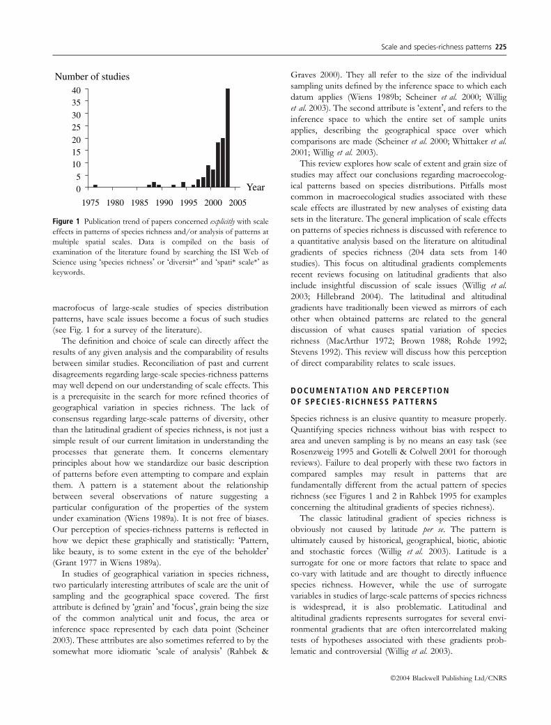
pattern becomes even more pronounced when only

�complete� gradients standardized for area effects and

sampling effort are considered (Fig. 4B). This increasing

frequency of hump-shaped patterns for �complete� gradients

and with greater altitudinal extent is not paralleled when

dividing the data sets into those obtained at a single, local,

transect and those compiled at a larger regional scale

(Fig. 4C and D). Considering all studies, a hump-shaped

pattern typically emerges both at the local and regional

extent. However, while this pattern becomes very pro-

nounced when considering only �complete� gradients stan-

dardized for area and sampling effort at the local scale, it

disappears entirely at the regional scale.

The extent of latitudinal and altitudinal gradients

The hidden and implicit assumption in most of the literature

dealing with both latitudinal and altitudinal species-richness

0

25

50

75

D Fd Hs Ho In O0

25

50

75

D Fd Hs Ho In O0

25

50

75

D Fd Hs Ho In O

0

25

50

75

D Fd Hs Ho In O0

25

50

75

D Fd Hs Ho In O0

25

50

75

D Fd Hs Ho In O

All studies Shortened gradients Complete gradients

Num

ber

of

un-s

tand

ardi

zed

stud

ies

Num

ber

of

stan

dard

ized

stu

dies

n = 204

n = 71 n = 124

n = 60 n = 110

n = 32

InvertebratesPlants Vertebrates

(A) (C)

(B) (D)

(E)

(F)

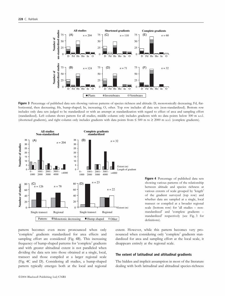
Figure 3 Percentage of published data sets showing various patterns of species richness and altitude: D, monotonically decreasing; Fd, flat-

horizontal, then decreasing; Hs, hump-shaped; In, increasing; O, other. Top row includes all data sets (non-standardized). Bottom row

includes only data sets judged to be standardized or with an attempt at standardization with regard to effect of area and sampling effort

(standardized). Left column shows pattern for all studies, middle column only includes gradients with no data points below 500 m a.s.l.

(shortened gradients), and right column only includes gradients with data points from £ 500 m to ‡ 2000 m a.s.l. (complete gradients).

Monotonic decreasing Hump–shaped OtherPattern: Monotonic decreasing Hump–shaped OtherPattern:

0

5

10

15

20

25

30

35

0

5

10

15

20

25

30

35

3001–4000

0–1000

1001–2000

2001–3000

>4000 3001–4000

0–1000

1001–2000

2001–3000

>4000

Complete gradientsstandardized

All studiesNon-standardized

n = 32n = 204

0

20

40

60

80

Single transect Regional

0

20

40

60

80

Single transect Regional

Monotonic decreasing Hump–shaped OtherPattern: Monotonic decreasing Hump-shaped OtherPattern:

n = 126 n = 78n = 23

Extent (m)

n = 22

Extent (m)Length of gradient

(A) (B)

(C) (D)

Num

ber

of s

tudi

esN

umbe

r of

stu

dies

Figure 4 Percentage of published data sets

showing various patterns of the relationship

between altitude and species richness at

various extents of scale grouped by �length�of the gradient surveyed (top row) and

whether data are sampled at a single, local

transect or compiled at a broader regional

scale (bottom row) for �all studies – non-

standardized� and �complete gradients –

standardized� respectively (see Fig. 3 for

definitions).

228 C. Rahbek


gradients is that these gradients are scale invariant as far as

mechanisms and processes determining variation in level of

species richness are concerned. Results obtained at both

gradients are thus viewed as directly comparable (MacArthur

1972; Brown 1988; Rohde 1992; Stevens 1992). This is,

however, a dubious assumption because of the difference in

extent of the two gradients (Rahbek 1997).

Complete latitudinal gradients span in excess of

10 000 km, whereas complete altitudinal (or depth) gradi-

ents rarely exceed a few kilometres, a difference of several

orders of magnitude. As a consequence, the impact of

historical and ecological mechanisms along the relatively

short altitudinal gradients is likely to be different from those

that operate along latitudinal gradients. Most species have a

significantly larger distributional extent along latitudinal

gradients than along altitudinal gradients. A greater range,

ceteris paribus, increases the chance of allopatric speciation

while reducing the risk of extinction (Rosenzweig 1992,

1995). For a species to persist within a given area there are

lower limits to population size, as well as upper limits on

population density.

Areas defined climatically by, for example, a fixed range

of temperatures, are dramatically smaller along altitudinal

gradients than latitudinal gradients. The conical shape of

mountains means that the influence of altitude is compoun-

ded by one of area, and generally, area decreases rapidly with

increasing altitude (MacArthur 1972; Lomolino 2001; Jones

et al. 2003). However, in vast mountain ranges such as the

Andes, altitudinal band areas are often narrowest at mid-

altitude (Rahbek 1997). Many species particularly of

vertebrates and vascular plants living in mountain habitats

are probably incapable of maintaining viable populations

within a single altitudinal band roughly characterized by

uniform abiotic living conditions (approximate band widths

of typically up to a few hundred metres). Thus, while the

grain size of individual latitudinal band areas is unlikely to

impose significant constraints on population viability per se,

and thereby on the distribution of species, the size of

climatically equivalent altitudinal bands most certainly does

(Graves 1988). However, that is not to imply that the

altitudinal and latitudinal range of a given species is straight

forward correlated with altitudinal and latitudinal variation

in climate in the same manner. In fact, bird species of the

Andes with very narrow altitudinal range often have

relatively extensive latitudinal ranges indicating a historical

signature (speciation) in the distributions (Graves 1988).

Still the extremely short spatial extent of altitudinal

gradients can potentially trigger a situation where species-

richness patterns are significantly influenced by community-

structuring factors such as source-sink population dynamics

(Rahbek 1997; Kessler 2000; Lomolino 2001; Grytnes

2003a). In other words, modifying, biotic mechanisms are

more likely to influence the altitudinal gradient of species

richness than the pattern of species richness along the

extensive latitudinal gradient (see Brehm et al. 2003 for a

case study on geometrid moths along an Andean gradient).

This difference may well be the reason for the lack of a

uniform altitudinal pattern (Rahbek 1995; Grytnes 2003b;

Fig. 3) as documented for latitude (Willig et al. 2003;

Hillebrand 2004). This does not imply that the primary

mechanisms influencing spatial variation of species richness

along the two gradients cannot be the same.

SCALE E F F EC T S : GRA IN

The choice of scale of analysis (i.e. grain size) directly

influences our visual perception of spatial patterns of

species as illustrated in Fig. 5A. Additionally, the use of too

coarse a grain size results in an excessive loss of information

and causes spurious extrapolation of high species densities

in species-poor localities (Rahbek & Graves 2000; Fig. 5A).

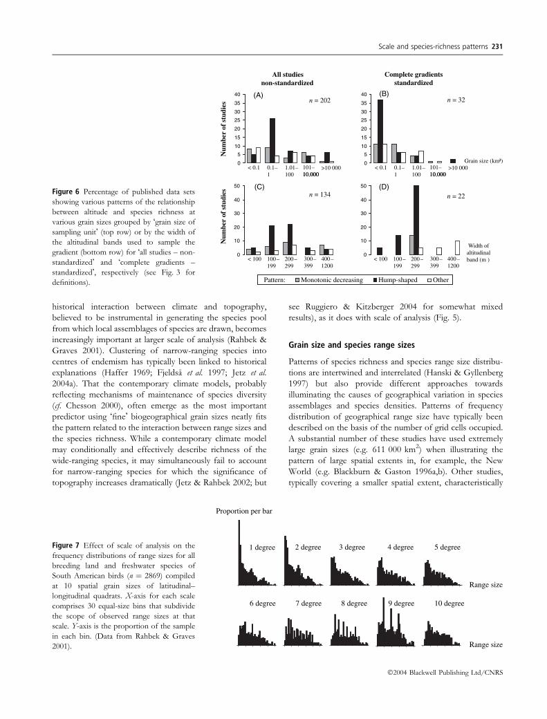
As Fig. 6 shows, the species-richness patterns for the

altitudinal gradient vary with grain size. At the smallest

grain-size (<0.1 km), hump-shaped patterns are relatively

less frequent than when data is sampled using larger grain

sizes (Fig. 6A). This may well be a sampling issue, as the

hump-shaped pattern dominates when only considering

�complete� gradients standardized for area and sampling

effort (Fig. 6B). Yet another distribution of shapes occurs

when tabulating patterns in classes of width of altitudinal

bands used to separate individual data points (Fig. 6C and

D). Here hump-shaped patterns dominate at intermediate

band size, especially when only considering �complete� and

standardized gradients, whereas a monotonic decreasing

pattern is very rare.

Grain size and our view of determinantsof species-richness patterns

Lyons & Willig (1999; see also Lyons & Willig 2002), in a

recent analysis of species-richness patterns of South

American bats and marsupials using nested quadrats of five

sizes ranging in area from 1000 to 25 000 km, showed that

the mechanisms believed to affect species richness are

indeed scale sensitive. A subsequent analysis of species

richness of South American hummingbirds at 10 spatial

scales spanning two orders of magnitude (quadrat size

c. 12 300–1 225 000 km2) found that the perception of

pattern and the conditional explanatory power of independ-

ent variables were directly dependent on the scale of analysis

(i.e. grain size; Rahbek & Graves 2000, 2001). These

findings were subsequently confirmed by other studies and

seem to be general (e.g. van Rensburg et al. 2002; Blackburn

et al. 2004).

At the continental extent, using �fine� biogeographical

grain sizes in contemporary climate-related models typically



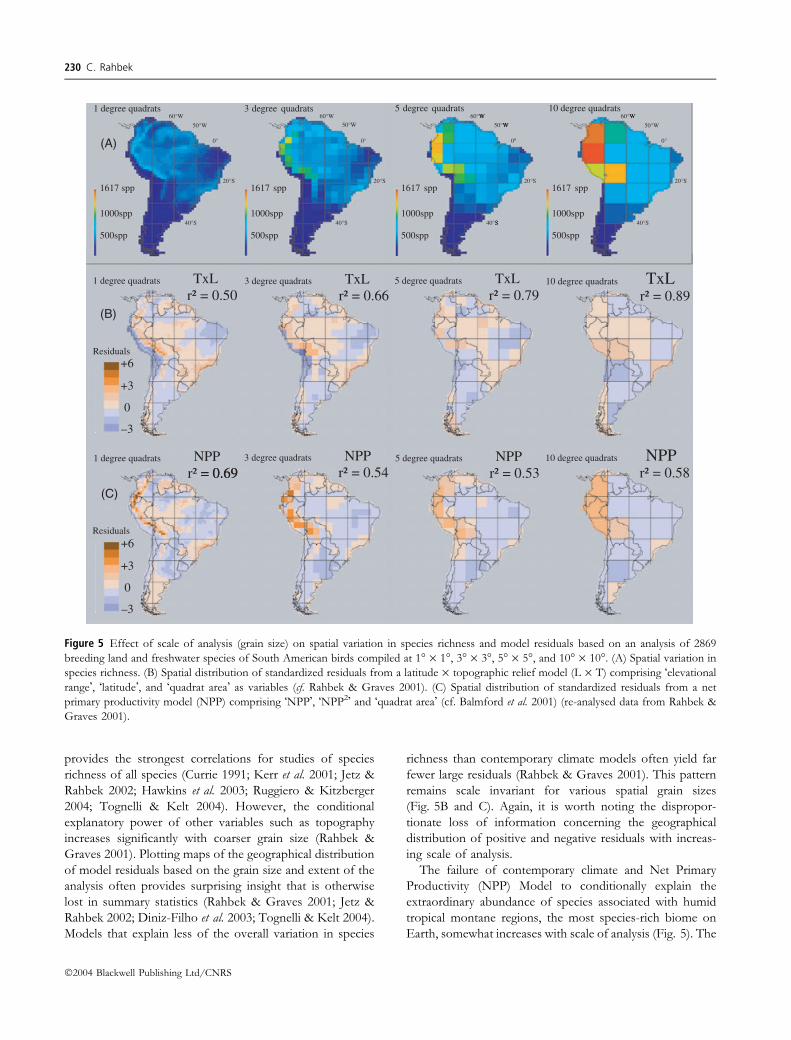
provides the strongest correlations for studies of species

richness of all species (Currie 1991; Kerr et al. 2001; Jetz &

Rahbek 2002; Hawkins et al. 2003; Ruggiero & Kitzberger

2004; Tognelli & Kelt 2004). However, the conditional

explanatory power of other variables such as topography

increases significantly with coarser grain size (Rahbek &

Graves 2001). Plotting maps of the geographical distribution

of model residuals based on the grain size and extent of the

analysis often provides surprising insight that is otherwise

lost in summary statistics (Rahbek & Graves 2001; Jetz &

Rahbek 2002; Diniz-Filho et al. 2003; Tognelli & Kelt 2004).

Models that explain less of the overall variation in species

richness than contemporary climate models often yield far

fewer large residuals (Rahbek & Graves 2001). This pattern

remains scale invariant for various spatial grain sizes

(Fig. 5B and C). Again, it is worth noting the dispropor-

tionate loss of information concerning the geographical

distribution of positive and negative residuals with increas-

ing scale of analysis.

The failure of contemporary climate and Net Primary

Productivity (NPP) Model to conditionally explain the

extraordinary abundance of species associated with humid

tropical montane regions, the most species-rich biome on

Earth, somewhat increases with scale of analysis (Fig. 5). The

(B)

3 degree quadrats TxLr² = 0.66




0°

1 degree quadrats

1617 spp

1000spp

500spp

60°W

50°W

20°S

40°S

3 degree quadrats

1617 spp

1000spp

500spp

60°W

50°W

20°S

40°S

W

W

°

S

5 degree quadrats

1617 spp

1000spp

500spp

60°W

50°W

0°

20°S

40°S

W

1617 spp

1000spp

500spp

60°W

50°W

0°

20°S

40°S

= 0.691 degree quadrats NPP

r² = 0.693 degree quadrats NPP



r² = 0.58

Residuals

Residuals

(A)

(C)

0°

+6

0

–3

+3

+6

0

–3

+3

10 degree quadrats

Figure 5 Effect of scale of analysis (grain size) on spatial variation in species richness and model residuals based on an analysis of 2869

breeding land and freshwater species of South American birds compiled at 1� · 1�, 3� · 3�, 5� · 5�, and 10� · 10�. (A) Spatial variation in

species richness. (B) Spatial distribution of standardized residuals from a latitude · topographic relief model (L · T) comprising �elevational

range�, �latitude�, and �quadrat area� as variables (cf. Rahbek & Graves 2001). (C) Spatial distribution of standardized residuals from a net

primary productivity model (NPP) comprising �NPP�, �NPP2� and �quadrat area� (cf. Balmford et al. 2001) (re-analysed data from Rahbek &

Graves 2001).

230 C. Rahbek


historical interaction between climate and topography,

believed to be instrumental in generating the species pool

from which local assemblages of species are drawn, becomes

increasingly important at larger scale of analysis (Rahbek &

Graves 2001). Clustering of narrow-ranging species into

centres of endemism has typically been linked to historical

explanations (Haffer 1969; Fjeldsa et al. 1997; Jetz et al.

2004a). That the contemporary climate models, probably

reflecting mechanisms of maintenance of species diversity

(cf. Chesson 2000), often emerge as the most important

predictor using �fine� biogeographical grain sizes neatly fits

the pattern related to the interaction between range sizes and

the species richness. While a contemporary climate model

may conditionally and effectively describe richness of the

wide-ranging species, it may simultaneously fail to account

for narrow-ranging species for which the significance of

topography increases dramatically (Jetz & Rahbek 2002; but

see Ruggiero & Kitzberger 2004 for somewhat mixed

results), as it does with scale of analysis (Fig. 5).

Grain size and species range sizes

Patterns of species richness and species range size distribu-

tions are intertwined and interrelated (Hanski & Gyllenberg

1997) but also provide different approaches towards

illuminating the causes of geographical variation in species

assemblages and species densities. Patterns of frequency

distribution of geographical range size have typically been

described on the basis of the number of grid cells occupied.

A substantial number of these studies have used extremely

large grain sizes (e.g. 611 000 km2) when illustrating the

pattern of large spatial extents in, for example, the New

World (e.g. Blackburn & Gaston 1996a,b). Other studies,

typically covering a smaller spatial extent, characteristically

0

10

20

30

40

50

0

10

20

30

40

50

0

5

10

15

20

25

30

35

40

0

5

10

15

20

25

30

35

40

Complete gradientsstandardized

All studiesnon-standardized

n = 32n = 202

n = 134

Monotonic decreasing Hump-shaped OtherPattern:

Grain size (km²)

10,000101–10 000

< 0.1 0.1–1

1.01–100

>10 00010,000101–10 000

< 0.1 0.1–1

1.01–100

>10 000

300–399

< 100 100–199

200–299

400–1200

300–399

< 100 100–199

200–299

400–1200

Width of altitudinal band (m )

n = 22

(A) (B)

(D)(C)

Num

ber

of s

tudi

esN

umbe

r of

stu

diesFigure 6 Percentage of published data sets

showing various patterns of the relationship

between altitude and species richness at

various grain sizes grouped by �grain size of

sampling unit� (top row) or by the width of

the altitudinal bands used to sample the

gradient (bottom row) for �all studies – non-

standardized� and �complete gradients –

standardized�, respectively (see Fig. 3 for

definitions).

Proportion per bar

1 degree 2 degree 3 degree 4 degree 5 degree

Range size

Range size

10 degree9 degree8 degree7 degree6 degree

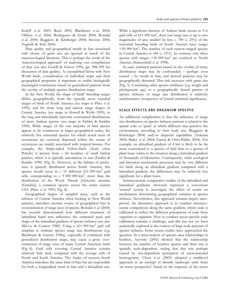
Figure 7 Effect of scale of analysis on the

frequency distributions of range sizes for all

breeding land and freshwater species of

South American birds (n ¼ 2869) compiled

at 10 spatial grain sizes of latitudinal–

longitudinal quadrats. X-axis for each scale

comprises 30 equal-size bins that subdivide

the scope of observed range sizes at that

scale. Y-axis is the proportion of the sample

in each bin. (Data from Rahbek & Graves

2001).



use grain sizes several times smaller than 611 000 km2

quadrats when measuring species range sizes, for example,

10 · 10 km grids for British birds (Gaston et al. 1998) or

50 · 50 km grids for European birds (Gregory et al. 1998).

Routinely, when discussing the general pattern of range-

size frequency distribution from such an array of studies, the

potential scale effect of extent is considered (Gaston &

Blackburn 2000), while the scale effect of grain size is

ignored. The tendency in the macroecological literature to

ignore the effect of grain size is peculiar, given the obvious

and enormous impact of this effect, especially because its

direct influence on our perception of species occurrences

per se is well described in the ecological literature (e.g. Levin

1992; Kunin 1998).

Range-size frequency distributions are not scale inde-

pendent, but can vary significantly even when sampling the

same distributions as a function of both grain size and

species richness (Fig. 7; see also Figs 5 and 8). Grain size

interacts with species distributions to produce different

patterns at different scales. This in itself is not a bias.

However, it certainly calls for caution when comparing data

among studies conducted at different scale of analysis or

when attempting to generalize from results of one study. In

addition, mean, median and modal range size constitute an

increasingly larger proportion of the total area of extent as

grain size increases, indicating that the signal-to-noise ratio

is inversely proportional to grain size (G.R. Graves and

C. Rahbek unpublished data). The use of very coarse grain

size to sample and describe geographical patterns of range

size distributions may thus result in gross overgeneraliza-

tions (see also Fig. 8).

Grain size and geographical trends in bias

Generated patterns of species richness or range-size

distributions using very coarse grain size are potentially

influenced by geographical trends in bias, which comes in

two forms: shape of range and apparent area of

occurrence relative to grain size (i.e. the signal-to-noise

ratio). This is especially true for the many species with

relatively small or linear geographical ranges. Such species

represent a significant proportion of taxa of the Neotrop-

ics in the New World, which in recent years has been used

as one of the most common templates for macroecological

studies of patterns of species richness and range size

distributions (e.g. Lyons & Willig 1997, 1999, 2002; Willig

& Lyons 1998; Gaston & Blackburn 2000; Rahbek &

Graves 2000, 2001; Cardillo 2002; Husak & Husak 2003;

of occupied Estimated range size (# of occupied cells)

Using grain size km²611 000 10 000

Hylocichla mustelina

Euphonia hirundinacea

Metallura tyrianthina

Sicalis citrina

12 550

7 96

Species ranges

10 72

15 62

Range size

60º 0

15Range size

60º 0

600

Latitudinal center of distribution

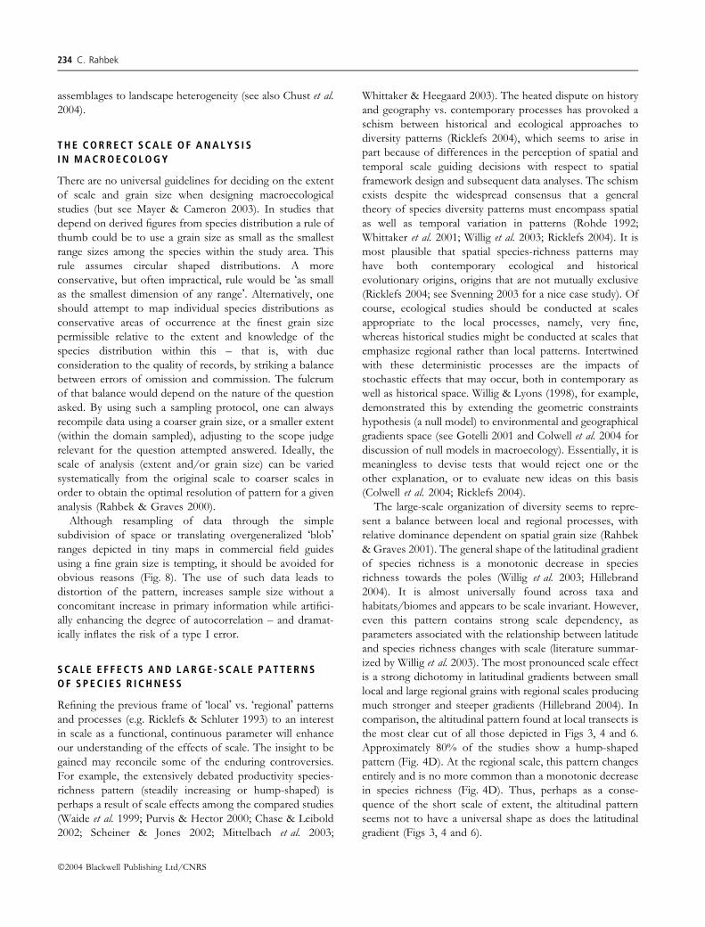
Figure 8 Effect of grain size on estimation of range sizes and geographical range-size patterns. The geographical distribution of four bird

species is illustrated (left map), each representing typical distributions in different biogeographical areas of the New World and their estimated

range size using quadrats of c. 611 000 and 10 000 km2 (right two columns) respectively (see text for discussion). The two small histograms

graphically illustrate how the perception of relative range sizes of the four species shifts with grain size. Consequently, a bias in perception of

latitudinal range-size frequency distributions can result from use of inappropriate grain size.

232 C. Rahbek


Koleff et al. 2003; Reed 2003; Blackburn et al. 2004;

Olifiers et al. 2004; Rodriguero & Gorla 2004; Romdal

et al. 2004; Ruggiero & Kitzberger 2004; Stevens 2004;

Tognelli & Kelt 2004).

Data quality and geographical trends in bias associated

with choice of grain size are ignored in much of the

macroecological literature. This is perhaps the result of the

�macroecological approach� of analysing vast compilations

of data (see also Gotelli & Graves 1996, pp. 308–309 for

discussion of data quality). As exemplified below with New

World birds, consideration of individual maps and their

geographical properties is important to enable biologically

meaningful conclusions based on generalized patterns from

the overlay of multiple species distribution maps.

In the New World, the shape of birds� breeding ranges

differs geographically, from the typically more rounded

ranges of birds of North America (see maps in Price et al.

1995), and the more long and narrow range shapes of

Central America (see maps in Howell & Webb 1995), to

the long and altitudinally narrowly constrained distributions

of most Andean species (see maps in Fjeldsa & Krabbe

1990). While ranges of the vast majority of bird species

appear to be continuous at larger geographical scales, the

relatively few terrestrial species for which actual areas of

occurrence are extensively dispersed within the extent of

occurrence are mainly associated with tropical biomes. For

example, the Stripe-tailed Yellow-finch (Sicalis citrina

Pelzeln) is known from c. 60 localities of small habitat

patches, where it is typically uncommon or rare (Fjeldsa &

Krabbe 1990) (Fig. 8). However, as the habitat of prefer-

ence is sparsely distributed across South America, this

species would occur in c. 15 different 611 000 km2 grid

cells, corresponding to c. 9 000 000 km2, more than the

distribution of the Wood Thrush [Hylocichla mustelina

(Gmelin)], a common species across the entire eastern

USA (Price et al. 1995; Fig. 8).

Geographical shapes of sampled areas, such as the

isthmus of Central America when looking at New World

patterns, introduce another source of geographical bias in

overestimation of range sizes of species. Romdal et al. (2004)

has recently demonstrated how different treatment of

latitudinal band area influences the estimated peak and

shape of the latitudinal gradient of species richness (see also

McCoy & Connor 1980). Using a 611 000 km2 grid cell

template to estimate species range size distributions (e.g.

Blackburn & Gaston 1996a), especially if combined with

generalized distribution maps, may cause a gross over-

estimation of range sizes of many Central American birds

(Fig. 8). Grid cells covering Central America contain

relatively little land, compared with the average cells of

North and South America. The Andes of western South

America introduce the same kind of bias but are responsible

for both a longitudinal trend in bias and a latitudinal one.

While a significant fraction of Andean birds occurs in 3–6

grid cells of 611 000 km2, their real range size is up to two

magnitudes of area smaller! In fact, c. 700 (c. 25%) of the

terrestrial breeding birds of South America have ranges

<50 000 km2. The number of such narrow-ranged species

in Central America is 344 (c. 15%). In contrast, only three

species with ranges <50 000 km2 are confined to North

America (Stattersfield et al. 1998).

In sum, statistical patterns based on the overlay of many

distribution maps may be confounded – perhaps even

caused – by trends in bias, and derived patterns may be

geographically distorted. This risk increases with grain size

(Fig. 5). Correlating other species attributes (e.g. weight and

phylogenetic age) to a geographically biased pattern of

species richness or range size distribution is relatively

uninformative irrespective of formal statistical significance.

SCALE E F F EC T S ARE ORGAN I SM SPEC I F I C

An additional complication is that the influence of range

size distribution on species richness patterns is related to the

spatial scale or �grain� at which different taxa perceive the

environment, according to their body size (Ruggiero &

Kitzberger 2004) and/or dispersal capabilities (Aukema

2004; Bailey et al. 2004; Garcıa & Ortiz-Pulido 2004). For

example, an altitudinal gradient of 4 km is likely to be far

more constrained to a species of bird than to a species of

plant louse relative to the situation along a latitudinal gradient

of thousands of kilometres. Consequently, while ecological

and historical mechanistic processes may be very different

for birds along an altitudinal gradient compared with a

latitudinal gradient, the differences may be relatively less

significant for a plant louse.

Intrataxonomic comparative studies of the altitudinal and

latitudinal gradients obviously represent a convenient

�natural� system to investigate the effect of extent on

mechanisms determining geographical variation in species

richness. Nevertheless, this approach remains largely unex-

plored. An alternative approach is to conduct intertaxo-

nomic comparisons along the same gradient, where scale is

calibrated to reflect the different perceptions of scale from

organism to organism. How to conduct taxon-specific scale

calibration remains a challenge, and this has not yet been

analytically explored in the context of large-scale patterns of

species richness. Some recent studies have approached the

question. In a meta-analysis of species–area relationships in

benthos, Azovsky (2002) showed that the relationship

between the number of benthos species and their size is

spatially scale-dependent, stating that this was perhaps

caused by size-dependent perception of environmental

heterogeneity. Chust et al. (2003) adopted a multilevel

approach in an attempt to identify landscape units from

�an insect perspective� based on the response of the insect



assemblages to landscape heterogeneity (see also Chust et al.

2004).

THE CORRECT SCALE OF ANALYS I S

IN MACROECOLOGY

There are no universal guidelines for deciding on the extent

of scale and grain size when designing macroecological

studies (but see Mayer & Cameron 2003). In studies that

depend on derived figures from species distribution a rule of

thumb could be to use a grain size as small as the smallest

range sizes among the species within the study area. This

rule assumes circular shaped distributions. A more

conservative, but often impractical, rule would be �as small

as the smallest dimension of any range�. Alternatively, one

should attempt to map individual species distributions as

conservative areas of occurrence at the finest grain size

permissible relative to the extent and knowledge of the

species distribution within this – that is, with due

consideration to the quality of records, by striking a balance

between errors of omission and commission. The fulcrum

of that balance would depend on the nature of the question

asked. By using such a sampling protocol, one can always

recompile data using a coarser grain size, or a smaller extent

(within the domain sampled), adjusting to the scope judge

relevant for the question attempted answered. Ideally, the

scale of analysis (extent and/or grain size) can be varied

systematically from the original scale to coarser scales in

order to obtain the optimal resolution of pattern for a given

analysis (Rahbek & Graves 2000).

Although resampling of data through the simple

subdivision of space or translating overgeneralized �blob�ranges depicted in tiny maps in commercial field guides

using a fine grain size is tempting, it should be avoided for

obvious reasons (Fig. 8). The use of such data leads to

distortion of the pattern, increases sample size without a

concomitant increase in primary information while artifici-

ally enhancing the degree of autocorrelation – and dramat-

ically inflates the risk of a type I error.

SCALE E F F EC T S AND LARGE - SCALE PAT T ERNS

OF SPEC I E S R I CHNESS

Refining the previous frame of �local� vs. �regional� patterns

and processes (e.g. Ricklefs & Schluter 1993) to an interest

in scale as a functional, continuous parameter will enhance

our understanding of the effects of scale. The insight to be

gained may reconcile some of the enduring controversies.

For example, the extensively debated productivity species-

richness pattern (steadily increasing or hump-shaped) is

perhaps a result of scale effects among the compared studies

(Waide et al. 1999; Purvis & Hector 2000; Chase & Leibold

2002; Scheiner & Jones 2002; Mittelbach et al. 2003;

Whittaker & Heegaard 2003). The heated dispute on history

and geography vs. contemporary processes has provoked a

schism between historical and ecological approaches to

diversity patterns (Ricklefs 2004), which seems to arise in

part because of differences in the perception of spatial and

temporal scale guiding decisions with respect to spatial

framework design and subsequent data analyses. The schism

exists despite the widespread consensus that a general

theory of species diversity patterns must encompass spatial

as well as temporal variation in patterns (Rohde 1992;

Whittaker et al. 2001; Willig et al. 2003; Ricklefs 2004). It is

most plausible that spatial species-richness patterns may

have both contemporary ecological and historical

evolutionary origins, origins that are not mutually exclusive

(Ricklefs 2004; see Svenning 2003 for a nice case study). Of

course, ecological studies should be conducted at scales

appropriate to the local processes, namely, very fine,

whereas historical studies might be conducted at scales that

emphasize regional rather than local patterns. Intertwined

with these deterministic processes are the impacts of

stochastic effects that may occur, both in contemporary as

well as historical space. Willig & Lyons (1998), for example,

demonstrated this by extending the geometric constraints

hypothesis (a null model) to environmental and geographical

gradients space (see Gotelli 2001 and Colwell et al. 2004 for

discussion of null models in macroecology). Essentially, it is

meaningless to devise tests that would reject one or the

other explanation, or to evaluate new ideas on this basis

(Colwell et al. 2004; Ricklefs 2004).

The large-scale organization of diversity seems to repre-

sent a balance between local and regional processes, with

relative dominance dependent on spatial grain size (Rahbek

& Graves 2001). The general shape of the latitudinal gradient

of species richness is a monotonic decrease in species

richness towards the poles (Willig et al. 2003; Hillebrand

2004). It is almost universally found across taxa and

habitats/biomes and appears to be scale invariant. However,

even this pattern contains strong scale dependency, as

parameters associated with the relationship between latitude

and species richness changes with scale (literature summar-

ized by Willig et al. 2003). The most pronounced scale effect

is a strong dichotomy in latitudinal gradients between small

local and large regional grains with regional scales producing

much stronger and steeper gradients (Hillebrand 2004). In

comparison, the altitudinal pattern found at local transects is

the most clear cut of all those depicted in Figs 3, 4 and 6.

Approximately 80% of the studies show a hump-shaped

pattern (Fig. 4D). At the regional scale, this pattern changes

entirely and is no more common than a monotonic decrease

in species richness (Fig. 4D). Thus, perhaps as a conse-

quence of the short scale of extent, the altitudinal pattern

seems not to have a universal shape as does the latitudinal

gradient (Figs 3, 4 and 6).

234 C. Rahbek


Altitudinal gradients as a suitable model to study scaleeffects

As a result of this scale sensitivity, altitudinal gradients

appear to be an excellent choice to study the effects of scale

on patterns of species richness. Additionally, altitudinal

gradients are highly suitable for the study of contemporary

climate, history and stochastic factors, as these vary along

the altitudinal gradient itself and with the geographical

(latitudinal) position of the gradient. This highlights the

need for comparative studies, although they remain few and

very recent (e.g. Grytnes 2003b).

Undoubtedly, scale effects in patterns of species richness

are associated with underlying and intertwined gradients in

alpha, beta and perhaps gamma diversity (Willig et al. 2003;

Rodrıguez & Arita 2004). Measurement of these units is

influenced by area and sampling effort, which in principle

can be fairly well controlled (or their effect explored) at well-

executed field studies along altitudinal gradients. Hence, it is

surprising that only about half of the included studies on

altitudinal gradients attempt to deal with these two factors

(Fig. 3A and B). The number of �complete� and �standard-

ized� gradients is likewise astonishingly small (only 32 of

204; Fig. 3F).

Quantitative approaches as used here to elucidate

patterns, potentially combined with the use of more explicit

meta-analysis statistics (e.g. Hillebrand 2004), seem suitable

to provide a rough overview of patterns in the results of

published studies. Sadly, no factorial meta-analysis technique

is currently available (Hillebrand 2004). As variables

characterizing attributes of organisms, their environment

and scale are intercorrelated (Figs 3, 4 and 6), caution is

highly warranted when interpreting statistical results based

on meta-analysis. Again, comparative field studies of

altitudinal gradients seem a promising approach to help

identify the details of possible consistent pattern in scale

effects.

OUT LOOK

Traditional evaluation of hypotheses in large-scale, non-

experimental, macroecological studies typically depends on

deviations from a statistical null hypothesis. The results of

these evaluations are usually expressed in terms such as r2, r,

F, CV, slope and P-values. It should be recognized that

these values are scale sensitive and conditional on model

design (Palmer 1994; Willig & Lyons 1998; Rahbek &

Graves 2001; Lichstein et al. 2002; Lyons & Willig 2002; van

Rensburg et al. 2002; Diniz-Filho et al. 2003; see Cressie

1993 for additional statistical insight). This is a problem as

increased consistency in model evaluation is desirable to

provide a more robust platform for identifying areas of

disagreement among �competing� hypotheses. Another

major obstacle is autocorrelation. Spatial autocorrelation is

an inherent quality of biogeographical data (Rahbek &

Graves 2000; Pimm & Brown 2004). It is also an effect that

is often correlated with sample size. However, the non-

independency among data points violates basic assumptions

of standard regression models and affects P-values and

values of model parameters as well as model selection in

stepwise procedures (Cressie 1993; Lichstein et al. 2002;

Diniz-Filho et al. 2003; Tognelli & Kelt 2004). This makes

comparison of such studies difficult.

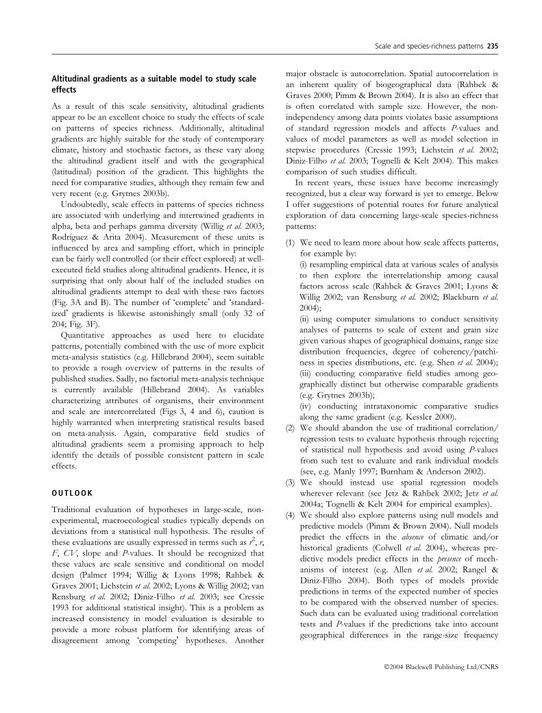
In recent years, these issues have become increasingly

recognized, but a clear way forward is yet to emerge. Below

I offer suggestions of potential routes for future analytical

exploration of data concerning large-scale species-richness

patterns:

(1) We need to learn more about how scale affects patterns,

for example by:

(i) resampling empirical data at various scales of analysis

to then explore the interrelationship among causal

factors across scale (Rahbek & Graves 2001; Lyons &

Willig 2002; van Rensburg et al. 2002; Blackburn et al.

2004);

(ii) using computer simulations to conduct sensitivity

analyses of patterns to scale of extent and grain size

given various shapes of geographical domains, range size

distribution frequencies, degree of coherency/patchi-

ness in species distributions, etc. (e.g. Shen et al. 2004);

(iii) conducting comparative field studies among geo-

graphically distinct but otherwise comparable gradients

(e.g. Grytnes 2003b);

(iv) conducting intrataxonomic comparative studies

along the same gradient (e.g. Kessler 2000).

(2) We should abandon the use of traditional correlation/

regression tests to evaluate hypothesis through rejecting

of statistical null hypothesis and avoid using P-values

from such test to evaluate and rank individual models

(see, e.g. Manly 1997; Burnham & Anderson 2002).

(3) We should instead use spatial regression models

wherever relevant (see Jetz & Rahbek 2002; Jetz et al.

2004a; Tognelli & Kelt 2004 for empirical examples).

(4) We should also explore patterns using null models and

predictive models (Pimm & Brown 2004). Null models

predict the effects in the absence of climatic and/or

historical gradients (Colwell et al. 2004), whereas pre-

dictive models predict effects in the presence of mech-

anisms of interest (e.g. Allen et al. 2002; Rangel &

Diniz-Filho 2004). Both types of models provide

predictions in terms of the expected number of species

to be compared with the observed number of species.

Such data can be evaluated using traditional correlation

tests and P-values if the predictions take into account

geographical differences in the range-size frequency



distribution of assemblages of species and the signature

of autocorrelation in the data.

(5) We should differentiate between local and global

approaches to spatial data analysis in ecology (Jetz et al.

2004b).

(6) Above all, we should avoid prejudgment regarding new

ideas and be open to new approaches, including those

deriving from other disciplines. For example, geograph-

ically weighted regression techniques (Fotheringham

et al. 2002), recently introduced by Foody (2004a) into

macroecology from geography, seem to be an interest-

ing supplement to spatial regression models. In partic-

ular, they may be a promising tool to elucidate local

performance of predictor variables and to explore spatial

non-stationarity and how that can give rise to varying

trends in scale dependence trends (Foody 2004b; Jetz

et al. 2004b). Note that this technique deals differently

with autocorrelation compared with spatial regression

techniques (Fotheringham et al. 2002) – an issue that

needs to be explored further (Foody 2004b).

Finally, it is necessary to consider how results vary as a

function of scale in order to put our knowledge regarding

patterns and processes into perspective. Obviously, this is a

necessary step, albeit only the initial one rather than the final

goal. In addition to asking how our results vary as a function

of scale, we should begin to search for consistent patterns in

these scale effects (Wiens 1989b). If we are to relate patterns

of diversity to scale in a way that elucidates the underlying

processes we will need to know more about the biological

underpinnings of variation in range size and ecological

specialization, as well as the role of geographical hetero-

geneity in generating regional species richness. Combining

sound statistical approaches with firm natural history

knowledge and knowledge about biological processes will,

eventually, enable us to attribute relative impact to various

factors and to decide at which point along a spatial and

temporal continuum they act.

ACKNOWLEDGEMENTS

For comments on drafts I would like to thank Robert K.

Colwell, Gary R. Graves, John-Arvid Grytnes, Helmut

Hillebrand, Michael Kessler, Christy M. McCain, Tom S.

Romdal, Kasper Thorup, and Michael Willig. I am also

grateful for the constructive comments by two anonymous

reviewers and the subject editor Boris Worm. I would

especially like to thank Gary R. Graves for discussions

throughout the years on these issues and Tom Romdal

for his critical contributions in compiling the data set for

the quantitative analysis. Frank Wugt Larsen helped

Tom in obtaining hardcopy versions of relevant papers.

P. Williams kindly provided the WORLDMAP software

used to manage the distributional data and to generate

Figs 5 and 8. The macroecological research work was

supported by the Danish National Science Foundation,

grant J. no. 21-03-0221.

RE F ERENCES

Abrams, P.A. (1995). Monotonic or unimodal diversity-produc-

tivity gradients: what does competition theory predicts. Ecology,

76, 2019–2027.

Allen, A.P., Brown, J.P. & Gillooly, J.F. (2002). Global biodiversity,

biochemical kinetics, and the energetic-equivalence rule. Science,

297, 1545–1548.

Aukema, J.E. (2004). Distribution and dispersal of desert

mistletoe is scale-dependent, hierarchically nested. Ecography, 27,

137–144.

Azovsky, A.I. (2002). Size-dependent species-area relationships in

benthos: is the world more diverse for microbes? Ecography, 25,

273–282.

Bachman, S., Baker, W.J., Brummitt, N., Dransfield, J. & Moat, J.

(2004). Elevational gradients, area and tropical island diversity:

an example from the palms of New Guinea. Ecography, 27,

299–310.

Bailey, S.A., Horner-Devine, M.C. & Luck, G., Moore, L.A.,

Carney, K.M., Anderson, S. et al. (2004). Primary productivity

and species richness: relationships among functional guilds,

residency groups and vagility classes at multiple spatial scales.

Ecography, 27, 207–217.

Balmford, A., Moore, J., Brooks, T., Burgess, N., Hansen, L.A.,

Williams, P. et al. (2001). Conservation conflicts across Africa.

Science, 291, 2616–2619.

Blackburn, T.M. & Gaston, K.J. (1996a). Spatial patterns in the

geographic range sizes of bird species in the New World. Phil.

Trans. R. Soc. B, 351, 897–912.

Blackburn, T.M. & Gaston, K.J. (1996b). Spatial patterns in

the species richness of birds in the New World. Ecography, 19,

369–376.

Blackburn, T.M. & Gaston, K.J. (2002). Scale in macroecology.

Global Ecol. Biogeogr., 11, 185–189.

Blackburn, T.M., Jones, K.E., Cassey, P. & Losin, N. (2004). The

influence of spatial resolution on macroecological patterns of

range size variation: a case study using parrot, Aves: Psittaci-

formes, of the world. J. Biogeogr., 31, 285–293.

Brehm, G., Sussenbach, D. & Fiedler, K. (2003). Unique eleva-

tional diversity patterns of geometrid moths in an Andean

montane rainforest. Ecography, 26, 456–466.

Brown, J.H. (1988). Species diversity. In: Analytical Biogeography –

An Integrated Approach to the Study of Animal and Plant Distribution

(eds Myers, A.A. & Giller, P.S.). Chapman and Hall, New York,

NY, pp. 57–89.

Brown, J.H. (1995). Macroecology. The University of Chicago Press,

London.

Brown, J.H. & Maurer, B.A. (1989). Macroecology – the division of

food and space among species on continents. Science, 243, 1145–

1150.

Burnham, K.P. & Anderson, D.R. (2002). Model Selection and Mul-

timodel Inference: A Practical Information–Theoretical Approach. Sprin-

ger-Verlag, New York, NY.

236 C. Rahbek


Cardillo, M. (2002). Body size and latitudinal gradients in regional

diversity of New World birds. Global Ecol. Biogeogr., 11, 59–65.

Chase, J.M. & Leibold, M.A. (2002). Spatial scale dictates the

productivity-biodiversity relationship. Nature, 416, 427–430.

Chesson, P. (2000). Mechanisms of maintenance of species

diversity. Annu. Rev. Ecol. Syst., 31, 343–366.

Chust, G., Pretus, J.L., Ducrot, D., Bedos, A. & Deharveng, L.

(2003). Identification of landscape units from an insect per-

spective. Ecography, 26, 257–268.

Chust, G., Pretus, J.L., Ducrot, D. & Ventura, D. (2004). Scale

dependency of insect assemblages in response to landscape

pattern. Lanscape Ecol., 19, 41–57.

Colwell, R.K., Rahbek, C. & Gotelli, N.J. (2004). The mid-domain

effect and species richness patterns: What have we learned so

far? Am. Nat., 163, 0E1–E23.

Cressie, N.A.C. (1993). Statistic for Spatial Data (Revised edn). Wiley,

Chichester, New York.

Currie, D.J. (1991). Energy and large-scale patterns of animal- and

plant-species richness. Am. Nat., 137, 27–49.

Diniz-Filho, J.A.F., Bini, L.M. & Hawkins, B.A. (2003). Spatial

autocorrelation and red herrings in geographical ecology. Global

Ecol. Biogeogr., 12, 53–64.

Fjeldsa, J. & Krabbe, N. (1990). Birds of the High Andes. Zoological

Museum, University of Copenhagen and Apollo Books,

Svendborg, Denmark.

Fjeldsa, J., Ehrlich, D., Lambin, E. & Prins, E. (1997). Are biodi-

versity ‘‘hotspots’’ correlated with current ecoclimatic stability?

A pilot study using NOAA-AVHRR remote sensing data. Biodiv.

Conserv., 6, 401–422.

Foody, G.M. (2004a). Spatial nonstationarity and scale-dependency

in the relationship between species richness and environmental

determinants for the sub-Saharan endemic avifauna. Global Ecol.

Biogeogr., 13, 315–320.

Foody, G.M. (2004b). Clarifications on local and global data ana-

lysis. Global Ecol. Biogeogr., in press.

Fotheringham, A.S., Brunsdon, C. & Charlton, M. (2002). Geo-

graphically Weighted Regression: The Analysis of Spatially Varying Re-

lationships. Wiley, Chichester, Hoboken, NJ.

Garcıa, D. & Ortiz-Pulido, R. (2004). Patterns of resource tracking

by avian frugivores at multiple spatial scales: two case studies on

discordance among scales. Ecography, 27, 187–196.

Gaston, K.J. & Blackburn, T.M. (1999). A critique for macro-

ecology. Oikos, 84, 353–368.

Gaston, K.J. & Blackburn, T.M. (2000). Pattern and Process in

Macroecology. Blackwell Science Ltd, Oxford.

Gaston, K.J., Quinn, R.M., Blackburn, T.M. & Eversham, B.C.

(1998). Species-range size distributions in Britain. Ecography, 21,

361–370.

Gotelli, N.J. (2001). Research frontiers in null model analysis.


Gotelli, N.J. & Colwell, R.K. (2001). Quantifying biodiversity:

procedures and pitfalls in the measurement and comparison of

species richness. Ecol. Lett., 4, 379–391.

Gotelli, N.J. & Graves, G.R. (1996). Null models in Ecology. Smith-

sonian Institution Press, Washington, DC.

Graves, G.R. (1988). Linearity of geographic range and its possible

effect on the population structure of Andean birds. Auk, 105,

47–52.

Gregory, R.D., Greenwood, J.J.D. & Hagemeijer, E.J.M. (1998).

The EBCC atlas of European breeding birds: a contribution to

science and conservation. Biologia E Conservazione Della Fauna,

102, 38–49.

Grytnes, J.A. (2003a). Ecological interpretations of the mid-domain

effect. Ecol. Lett., 6, 883–888.

Grytnes, J.A. (2003b). Species-richness patterns of vascular plants

along seven altitudinal transects in Norway. Ecography, 26, 291–

300.

Grytnes, J.A. & Vetaas, O.R. (2002). Species richness and altitude:

a comparison between null models and interpolated plant spe-

cies richness along the Himalayan altitudinal gradient, Nepal.

Am. Nat., 159, 294–304.

Haffer, J. (1969). Speciation in Amazonian forest birds. Science, 165,

131–137.

Hanski, I. & Gyllenberg, M. (1997). Uniting two general patterns in

the distribution of species. Science, 275, 387–400.

Hawkins, B.A., Porter, E.E. & Diniz-Filho, J.A.F. (2003). Pro-

ductivity and history as predictors of the latitudinal diversity

gradient of terrestrial birds. Ecology, 84, 1608–1623.

Hillebrand, H. (2004). On the generality of the latitudinal diversity

gradient. Am. Nat., 163, 192–211.

Howell, S.N.G. & Webb, S. (1995). The Birds of Mexico and Northern

Central America. Oxford University Press, Oxford.

Husak, M.S. & Husak, A.L. (2003). Latitudinal patterns in range

sizes of New World woodpeckers. Southwest. Nat., 48, 61–69.

Hutchinson, G.E. (1953). The concept of pattern in ecology. Proc.

Natl Acad. Sci. USA, 105, 1–12.

Hutchinson, G.E. (1959). Homage to Santa Rosalia, or ��why are

there so many kinds of animals?‘‘. Am. Nat., 93, 145–159.

Jetz, W. & Rahbek, C. (2002). Geographic range size and

determinants of avian species richness. Science, 297, 1548–1551.

Jetz, W., Rahbek, C. & Colwell, R.K. (2004a). Rarity, richness and the

signature of history in centers or endemism. Ecol. Lett., 7, 1180–

1191.

Jetz, W., Rahbek, C. & Lichstein, J.W. (2004b). Local and global

approaches to spatial data analysis in ecology. Global Ecol. Bio-

geogr., in press.

Jones, J.I., Li, W. & Maberly, S.C. (2003). Area, altitude and aquatic

plant diversity. Ecography, 26, 411–420.

Kerr, J.T., Southwood, T.R.E. & Cihlar, J. (2001). Remotely sensed

habitat diversity predicts butterfly species richness and com-

munity similarity in Canada. Proc. Natl Acad. Sci. USA, 98, 11365–

11370.

Kessler, M. (2000). Elevational gradients in species richness and

endemism of selected plant groups in the central Bolivian An-

des. Plant Ecol., 149, 181–193.

Koleff, P., Lennon, J.J. & Gaston, K.J. (2003). Are there latitudinal

gradients in species turnover?. Global Ecol. Biogeogr., 12, 483–498.

Kunin, W.E. (1998). Extrapolating species abundance across spatial

scales. Science, 281, 1513–1515.

Levin, S.A. (1992). The problem of pattern and scale in ecology.

Ecology, 73, 1943–1967.

Lichstein, J.W., Simons, T.R., Shriner, S.A. & Franzreb, K.E.

(2002). Spatial autocorrelation and autoregressive models in

ecology. Ecol. Monogr., 72, 445–463.

Lomolino, M.V. (2001). Elevation gradients of species-density:

historical and prospective views. Global Ecol. Biogeogr., 10,

3–13.

Lyons, S.K. & Willig, M.R. (1997). Latitudinal patterns of range

size: methodological concerns and empirical evaluations for

New World bats and marsupials. Oikos, 79, 568–580.



Lyons, S.K. & Willig, M.R. (1999). A hemispheric assessment of

scale-dependence in latitudinal gradients of species richness.

Ecology, 80, 2483–2491.

Lyons, S.K. & Willig, M.R. (2002). Species richness, latitude, and

scale-sensitivity. Ecology, 83, 47–58.

MacArthur, R.H. (1969). Patterns of communities in the tropics.

Biol. J. Linn. Soc. Lond., 1, 19–30.

MacArthur, R.H. (1972). Geographical Ecology. Harper and Rowe

Publishers, New York.

Manly, B.F.J. (1997). Randomization, Bootstrap and Monte Carlo Methods

in Biology. Chapman and Hall, London.

Mayer, A.L. & Cameron, G.N. (2003). Consideration of grain and

extent in landscape studies of terrestrial vertebrate ecology.

Landscape Urban Plan., 65, 201–217.

McCoy, E.D. (1990). The distribution of insects along elevational

gradients. Oikos, 58, 313–322.

McCoy, E.D & Connor, E.F. (1980). Latitudinal gradients in the

species diversity of North American mammals. Evolution, 34,

193–203.

Mittelbach, G.G., Scheiner, S.M. & Steiner, G.F. (2003). What is

the observed relationship between species richness and pro-

ductivity? Reply. Ecology, 84, 3390–3395.

Olifiers, N., Vieira, M.V. & Grelle, C.E.V. (2004). Geographic

range and body size in Neotropical marsupials. Global Ecol.

Biogeogr., 13, 439–444.

Orians, G.H. (1969). The number of bird species in some tropical

forests. Ecology, 50, 783–801.

Palmer, M.W. (1994). Variation in species richness: towards

a unification of hypotheses. Folia Geobot. Phytotaxon, 29, 511–

530.

Pimm, S.L. & Brown, J.H. (2004). Domains of diversity. Science,

304, 831–833.

Price, J., Droege, S. & Price, A. (1995). The Summer Atlas of North

American Birds. Academy Press, San Diego, CA.

Purvis, A. & Hector, A. (2000). Getting the measure of biodi-

versity. Nature, 405, 212–219.

Rahbek, C. (1995). The elevational gradient of species richness: a

uniform pattern?. Ecography, 18, 200–205.

Rahbek, C. (1997). The relationship among area, elevation, and

regional species richness in Neotropical birds. Am. Nat., 149,

875–902.

Rahbek, C. & Graves, G.R. (2000). Detection of macro-ecolo-

gical patterns in South American hummingbirds is affected

by spatial scale. Proc. R. Soc. Lond. B. Biol. Sci., 267, 2259–

2265.

Rahbek, C. & Graves, G.R. (2001). Multiscale assessment of pat-

terns of avian species richness. Proc. Natl Acad. Sci. USA, 98,

4534–4539.

Rangel, T.F.L.V.B. & Diniz-Filho, J.A. (2004). An evolutionary

tolerance model explaining spatial patterns in species richness

under environmental gradients and geometric constraints. Eco-

graphy, in press.

Reed, R.N. (2003). Interspecific patterns of species richness, geo-

graphic range size, and body size among New World venomous

snakes. Ecography, 26, 107–117.

van Rensburg, B.J., Chown, S.L. & Gaston, K.J. (2002). Species

richness, environmental correlates, and spatial scale: a test using

South African birds. Am. Nat., 159, 566–577.

Ricklefs, R.E. (1987). Community diversity: relative roles of local

and regional processes. Science, 235, 167–171.

Ricklefs, R.E. (2004). A comprehensive framework for global

patterns in biodiversity. Ecol. Lett., 7, 1–15.

Ricklefs, R.E. & Schluter, D., eds (1993). Species Diversity in Ecological

Communities: Historical and Geographical Perspectives. University of

Chicago Press, Chicago, IL.

Rodriguero, M.S. & Gorla, D.E. (2004). Latitudinal gradient in

species richness of the New World Triatominae (Reduviidae).


Rodrıguez, P. & Arita, H.T. (2004). Beta diversity and latitude in

North American mammals: testing the hypothesis of covaria-

tion. Ecography, 27, 547–556.

Rohde, K. (1992). Latitudinal gradients in species diversity: the

search for the primary cause. Oikos, 65, 514–527.

Romdal, T.S., Colwell, R.K. & Rahbek, C. (2004). The influence of

band sum area, domain extent and range sizes on the latitudinal

mid-domain effect. Ecology, in press.

Rosenzweig, M.L. (1992). Species diversity gradients: we know

more and less than we thought. J. Mamm., 73, 715–730.

Rosenzweig, M.L. (1995). Species Diversity in Space and Time. Cam-

bridge University Press, New York, NY.

Ruggiero, A. & Kitzberger, T. (2004). Environmental correlates of

mammal species richness in South America: effects of spatial

structure, taxonomy and geographic range.Ecography, 27, 401–416.

Scheiner, S.M. (2003). Six types of species-area curves. Global Ecol.

Biogeogr., 12, 441–447.

Scheiner, S.M. & Jones, S. (2002). Diversity, productivity and scale

in Wisconsin vegetation. Evol. Ecol. Res., 4, 1097–1117.

Scheiner, S.M., Cox, S.B., Willig, M.R., Mittlebach, G.G., Osen-

berg, C.W. & Kaspari, M. (2000). Species richness: scale effects

and Simpson’s paradox. Evol. Ecol. Res., 2, 791–802.

Schneider, D.C. (1994). Quantitative Ecology: Spatial and Temporal

Scaling. Academic Press, San Diego, CA.

Shen, W., Jenerette, G.D., Wu, J. & Gardner, R.H. (2004). Eval-

uating empirical scaling relations of pattern metrics with simu-

lated landscapes. Ecography, 27, 459–469.

Stattersfield, A.J., Crosby, M.J., Long, A.J. & Wege, D.C. (1998).

Endemic Bird Areas of the World. Priorities for Biodiversity Conservation.

BirdLife International, Cambridge.

Stevens, G.C. (1989). The latitudinal gradient in geographical range:

how so many species coexist in the tropics. Am. Nat., 133, 240–

256.

Stevens, G.C. (1992). The elevational gradient in altitudinal range:

an extension of Rapoport’s latitudinal rule to altitude. Am. Nat.,

140, 893–911.

Stevens, R.D. (2004). Untangling latitudinal richness gradients at

higher taxonomic levels: familial perspectives on the diversity of

New World bat communities. J. Biogeogr., 31, 665–674.

Svenning, J.C. (2003). Deterministic Plio-Pleistocene extinctions in

the European cool-temperate tree flora. Ecol. Lett., 6, 646–653.

Terborgh, J. (1971). Distribution on environmental gradients: theory

and a preliminary interpretation of distributional patterns in the

avifauna of the Cordillera Vilcabamba, Peru. Ecology, 52, 23–40.

Tognelli, M.F. & Kelt, D.A. (2004). Analysis of determinants of

mammalian species richness in South America using spatial au-

toregressive models. Ecography, 27, 427–436.

Waide, R.B., Willig, M.R., Steiner, C.F., Mittelbach, G., Gough, L.,

Dodson, S.I. et al. (1999). The relationship between productivity

and species Richness. Annu. Rev. Ecol. Syst., 130, 257–300.

Whittaker, R.H. (1977). Evolution of species diversity in land

communities. Evol. Biol., 10, 1–67.

238 C. Rahbek


Whittaker, R.J. & Heegaard, E. (2003). What is the observed

relationship between species richness and productivity?

Comment. Ecology, 84, 3384–3390.

Whittaker, R.J., Willis, K.J. & Field, R. (2001). Scale and species

richness: towards a general, hierarchical theory of species

diversity. J. Biogeogr., 28, 453–470.

Wiens, J.A. (1989a). The Ecology of Bird Communities: Foundations and

Patterns, Vol. 1. University Press, Cambridge.

Wiens, J.A. (1989b). Spatial scaling in ecology. Funct. Ecol., 3, 385–

397.

Wiens, J.A., Rotenberry, J.T. & Van Horne, B. (1987). Habitat

occupancy patterns of North American shrubsteppe birds: the

effect of spatial scale. Oikos, 48, 132–147.

Willig, M.R. & Lyons, S.K. (1998). An analytical model of latitude

gradients of species richness with an empirical test for marsu-

pials and bats in the New World. Oikos, 81, 93–98.

Willig, M.R., Kaufman, D.M. & Stevens, R.D. (2003). Latitudinal

gradients of biodiversity: pattern, process, scale and synthesis.

Annu. Rev. Ecol. Evol. Syst., 34, 273–309.

Willis, K.J. & Whittaker, R.J. (2002). Species diversity-scale matters.

Science, 295, 1245–1248.

Wright, D.H. (1983). Species-energy theory: an extension of

species-area theory. Oikos, 41, 496–506.

Editor, Boris Worm

Manuscript received 30 April 2004

First decision made 24 June 2004

Second decision made 13 September 2004

Manuscript accepted 21 September 2004



Ecology Letters, (2005) 8: 224–239 doi: 10.1111/j.1461...

Documents

Transcript of Ecology Letters, (2005) 8: 224–239 doi: 10.1111/j.1461...