Ecological Evaluation Technical Guidance · ECSM Ecological Conceptual Site Model . EE Ecological...
139
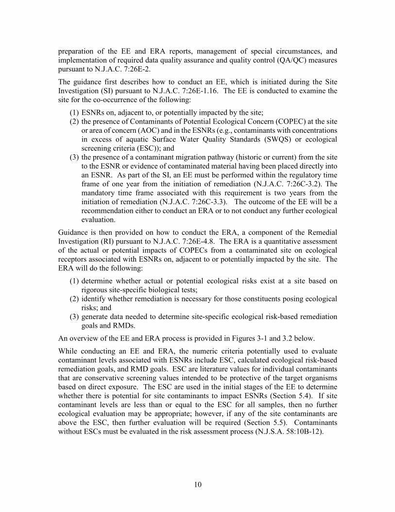
Ecological Evaluation Technical Guidance New Jersey Department of Environmental Protection Site Remediation and Waste Management Program August 2018 Version 2.0
Transcript of Ecological Evaluation Technical Guidance · ECSM Ecological Conceptual Site Model . EE Ecological...
Ecological Evaluation Technical Guidance
New Jersey Department of Environmental Protection
Site Remediation and Waste Management Program
August 2018
Version 2.0
2
Ecological Evaluation Technical Guidance Version 2.0
Table of Contents
Acronyms and Abbreviations ..............................................................................................5 Executive Summary .............................................................................................................7 1.0 Intended Use of Guidance Document ......................................................................... 8 2.0 Purpose ........................................................................................................................ 8 3.0 Document Overview ................................................................................................... 9 4.0 Definitions................................................................................................................. 12 5.0 Technical Guidance for Preparing Ecological Evaluations ...................................... 19
5.1 Ecological Evaluation Pursuant to N.J.A.C. 7:26E-1.16 .................................19 5.2 Ecological Evaluation Pursuant to N.J.A.C. 7:26E-4.8 ...................................20 5.2.1 Environmentally Sensitive Natural Resources ............................................20 5.2.2 Contaminants of Potential Ecological Concern ...........................................21 5.2.3 Contaminant Migration Pathways ...............................................................22
5.3 Recommended Sample Collection in Support of Ecological Evaluations .......22 5.3.1 When to Collect Samples ............................................................................23 5.3.2 Where to Collect Samples ...........................................................................24
5.3.2.1 Potential Contaminant Migration Pathways ......................................... 24 5.3.2.2 Environmentally Sensitive Natural Resources ...................................... 24
5.3.3 How to Collect Samples ..............................................................................27 5.3.3.1 Soils and Sediments .............................................................................. 27 5.3.3.2 Surface Water........................................................................................ 27
5.3.4 Background Considerations ........................................................................28 5.4 Comparison of Sample Data with Ecological Screening Criteria ....................29 5.4.1 Potential Migration Pathways .....................................................................30 5.4.2 Surface Water Bodies ..................................................................................30 5.4.3 Wetlands ......................................................................................................31 5.4.4 Uplands ........................................................................................................32
5.5 Ecological Evaluation Report ..........................................................................32 6.0 Technical Guidance for Preparing Ecological Risk Assessments ............................ 33
6.1 Ecological Risk Assessment Process Pursuant to N.J.A.C. 7:26E-4.8 ............33 6.1.1 Problem Formulation ...................................................................................35
6.1.1.1 Assessment and Measurement Endpoints ............................................. 35 6.1.1.2 Ecological Conceptual Site Model ........................................................ 38
6.1.2 Analysis .......................................................................................................39 6.1.3 Risk Characterization ..................................................................................39
6.1.3.1 Food Chain Modeling ........................................................................... 40 6.1.3.2 Bioaccumulation ................................................................................... 44 6.1.3.3 Toxicity Reference Values .................................................................... 50 6.1.3.4 Weight-of-Evidence .............................................................................. 52
6.2 ERA Data Development ..................................................................................53 6.2.1 Surface Water ..............................................................................................54
6.2.1.1 Sampling Plan Design for Study and Reference Areas ........................ 54 6.2.1.2 Surface Water Habitat Assessments and Community Surveys............. 55
3
6.2.1.3 Biological Sampling of Fish and Other Aquatic Organisms ................ 57 6.2.1.4 Surface Water Toxicity Tests................................................................ 59
6.2.2 Sediments ....................................................................................................60 6.2.2.1 Sampling Plan Design for Study and Reference Areas ........................ 60 6.2.2.2 Sediment Habitat Assessments and Community Surveys .................... 63 6.2.2.3 Sediment Pore Water Sampling ............................................................ 64 6.2.2.4 Benthic Macroinvertebrate Sampling ................................................... 66 6.2.2.5 Sediment Toxicity Tests ....................................................................... 67 6.2.2.6 Toxicity Testing for Sediment Pore Water and Elutriate ...................... 67
6.2.3 Soil 68 6.2.3.1 Sampling Plan Design for Study and Reference Areas ........................ 68 6.2.3.2 Terrestrial Habitat Assessments and Community Surveys ................... 70 6.2.3.3 Surface Soil Sampling........................................................................... 71 6.2.3.4 Biological Sampling of Soil Invertebrates, Plants and Wildlife ........... 71 6.2.3.5 Surface Soil Toxicity Tests ................................................................... 73
6.3 Ecological Risk Assessment Report ................................................................73 6.4 Special Circumstances .....................................................................................74 6.4.1 Wetlands ......................................................................................................74
6.4.1.1 Wetland Permit Considerations ............................................................ 76 6.4.1.2 Wetland Backfill Considerations .......................................................... 77
6.4.2 Estuaries ......................................................................................................77 6.4.3 Urban Areas .................................................................................................78 6.4.4 Hot Spots .....................................................................................................78 6.4.5 Extractable Petroleum Hydrocarbons ..........................................................78 6.4.6 Polycyclic Aromatic Hydrocarbons ............................................................79 6.4.7 Polychlorinated Biphenyls (Aroclor vs. Congener) ....................................81 6.4.8 Chlorinated Dioxin, Furans, and Dioxin-like Polychlorinated Biphenyls ..82 6.4.9 Historic Fill Material and Dredged Material ...............................................84 6.4.10 Acid-Volatile Sulfides/Simultaneously Extracted Metals ...........................85 6.4.11 Guidance for the Evaluation of Mercury Contaminated Sites ....................86
7.0 Determination of Ecological Risk-Based Remediation Goals .................................. 87 7.1 Use of Food Chain Models and Tissue Residue Data to Determine
Remediation Goals ...........................................................................................88 7.2 Use of Soil and Sediment Toxicity Test Results to Determine Remediation
Goals ................................................................................................................89 7.2.1 Apparent Effects Threshold Approach ........................................................89 7.2.2 Sediment/Soil Effects Concentration Approach ..........................................89
7.3 Application of Ecological Remediation Goals ................................................90 8.0 Uncertainty ................................................................................................................ 90 9.0 Risk Management Considerations ............................................................................ 91
9.1 Soil Remediation Standards and Deed Notices ...............................................91 9.2 Risk Management Decisions............................................................................92
10.0 Quality Assurance/Quality Control and Data Usability ............................................ 94 11.0 References ................................................................................................................. 95 Appendix A - Habitat Survey Forms ...............................................................................111 Appendix B - Sampling Procedures for Benthic Algae and Plankton .............................115
4
Appendix C - Surface Water Toxicity Testing ................................................................117 Appendix D - Sediment Toxicity Testing ........................................................................121 Appendix E - Sediment Pore Water and Elutriate Toxicity Testing ................................125 Appendix F – Sediment Pore Water Sampling Techniques .............................................128 Appendix G – Invertebrate Sampling Methods ...............................................................130 Appendix H - Soil Toxicity Testing.................................................................................133 Appendix I - Using the Toxic Equivalency (TEQ) Approach to Evaluate Dioxin, Furan,
and Dioxin-like PCB Results ....................................................................136
Tables and Figures
Figure 3-1: Flow diagram to describe the EE process during the Site Investigation .......11
Figure 3-2: Flow diagram to describe the EE and ERA process in the Remedial Investigation ..................................................................................................12
Figure 5-1: Sketch map of river showing stratified regions and sampling points ...........26
Figure 6-1: Assessment and Measurement Endpoints .....................................................37
Figure 6-2: Ecological Conceptual Site Model ................................................................38
Figure 6-3: Example of an Ecological Conceptual Site Model as a Chart ......................39
Table 1: Summary of TRVs for Avian and Mammalian Wildlife Receptors from the Passaic River FFS...........................................................................52
Figure 6-4: Conceptual Model for Applying Various Sediment Assessment Approaches in a Tiered System to Determine the Risk of Adverse Effects Due to PAHs in Sediments ...............................................................80
Figure 7-1: Hypothetical Example of Media Concentrations to Consider for Selection of Ecological Risk-Based Remediation Goals ..............................87
Figure 7-2: Simplified Example of Determining a Remediation Goal Using a Standard Food Chain Model and Site-Specific Tissue Residue Data ...........88
Figure 7-3: Simplified Example of Determining a Remediation Goal Using the Apparent Effects Threshold (AET) Approach ..............................................89
Figure 9-1: Plot of Exposure Risk Reduction vs. Acres of Habitat Destroyed ...............93
Cover Photo: Black-crowned Night-Heron, courtesy of Michael Mandracchia
5
Acronyms and Abbreviations ADD Average Daily Dose (mg/kg-day) AET Apparent Effects Threshold AF Absorption Fraction AFDW Ash-Free Dry Weight ASTM American Society for Testing and Materials AVS Acid Volatile Sulfide BERA Baseline Ecological Risk Assessment BAF Bioaccumulation Factor BSAFs Biota-Sediment/Soil Accumulation Factors BW Body weight CERCLA Comprehensive Environmental Response, Compensation, and Liability Act CM Concentration of COPECs in media of concern COPEC Contaminants of Potential Ecological Concern CR Contact Rates (kg/day or L/day) CSM Conceptual Site Model DDT Dichloro-Diphenyl, Tri-Chloroethane DGT Diffusive Gradient in Thin Films DO Dissolved Oxygen DQO Data Quality Objectives EcoSSLs Ecological Soil Screening Levels ECSM Ecological Conceptual Site Model EE Ecological Evaluation EqP Equilibrium Partitioning ERA Ecological Risk Assessments ERAGS Ecological Risk Assessment Guidance for Superfund: Process for
Designing and Conducting Ecological Risk Assessments (EPA 540-R-97-006, June 1997)
ER-L Effects Range-Low ER-M Effects Range-Median ESC Ecological Screening Criteria ESNR Environmentally Sensitive Natural Resource FI Fractional Intake FSPM Field Sampling Procedures Manual GIS Geographic Information System HOC Hydrophobic Organic Chemical HQ Hazard Quotient IC Inhibitory Concentration ITRC Interstate Technology & Regulatory Council LEL Lowest Effects Level LOAEL Lowest Observed Adverse Effect Level LOEC Lowest Observed Effect Concentration LOI Letter of Interpretation LSRP Licensed Site Remediation Professional MDL Method Detection Limit mg/l CaCO3 Milligrams Per Liter of Calcium Carbonate (Hardness)

6
NELAP National Environmental Laboratory Accreditation Program N.J.A.C. New Jersey Administrative Code NJDEP New Jersey Department of Environmental Protection NJPDES New Jersey Pollutant Discharge Elimination System NOAEL No Observed Adverse Effect Level NOEC No Observed Effect Concentration OSWER Office of Solid Waste and Emergency Response PAH Polycyclic Aromatic Hydrocarbon PCB Polychlorinated Biphenyls PCDD Polychlorinated Dibenzo-P-Dioxins PCDF Polychlorinated Dibenzofuran PE Polyethylene pg/ml Picogram/Milliliter POM Polyoxymethylene ppm Part Per Million ppt Part Per Trillion or Part Per Thousand for salinity QA/QC Quality Assurance and Quality Control QAPP Quality Assurance Project Plan RBP Rapid Bioassessment Protocols RMD Risk Management Decision ROI Receptors of Interest SEC Sediment/Soil Effects Concentration SEL Severe Effects Level SEM Simultaneously Extracted Metals SI Site Investigation SLERA Screening Level Ecological Risk Assessment SMDP Scientific/Management Decision Point SPMD Semi-Permeable Membrane Device SPME Solid Phase Microextraction Devices SRS Soil Remediation Standards SRT Standard Reference Toxicant SRWMP Site Remediation and Waste Management Program SWQS Surface Water Quality Standards (N.J.A.C. 7:9B) TEC Toxicity Equivalence Concentration TEF Toxic Equivalency Factor TEQ Toxic Equivalency TIC Tentatively Identified Contaminant TOC Total Organic Carbon TRV Toxicity Reference Value UCL Upper Confidence Limit U.S.C. United States Code USEPA United States Environmental Protection Agency USGS United States Geological Survey VOC Volatile Organic Compounds WET Whole Effluent Toxicity WHO World Health Organization
7
Executive Summary This document provides technical guidance on how to conduct an Ecological Evaluation (EE) and an Ecological Risk Assessment (ERA) pursuant to N.J.A.C. 7:26E-1.16 and N.J.A.C. 7:26E-4.8 for environmentally sensitive natural resources (ESNR) associated with contaminated sites. Guidance is also provided for the derivation of site-specific ecological risk-based remediation goals and Risk Management Decisions (RMD). Although the Licensed Site Remediation Professionals (LSRP) should understand the purpose and intent of this guidance, the investigator performing the EE and ERA must be experienced in the use of techniques and methodologies for conducting ERAs (N.J.S.A. 58:10C-16(c)) and must be able to comply with appropriate guidance including, but not limited to, USEPA’s Ecological Risk Assessment Guidance for Superfund, Process for Designing and Conducting Ecological Risk Assessments, EPA 540-R-97-006, Office of Solid Waste and Emergency Response, Washington, DC (ERAGS - USEPA, 1997a) (N.J.S.A. 58:10B-12). If the LSRP does not possess the necessary qualifications, subcontracting to qualified investigators is appropriate. This guidance was prepared in accordance with the Technical Requirements for Site Remediation, N.J.A.C. 7:26E, the Site Remediation Reform Act, N.J.S.A. 58:10C-1 et seq., and the Administrative Requirements for the Remediation of Contaminated Sites, N.J.A.C. 7:26C.
The EE is conducted to examine the site for the co-occurrence of the following:
(1) ESNRs on, adjacent to, or potentially impacted by the site, (2) the presence of Contaminants of Potential Ecological Concern (COPEC) at the site
or Area of Concern (AOC) and in the ESNRs, and (3) the presence of a contaminant migration pathway (historic or current) from the site
to the ESNR or evidence of contaminated material having been placed directly into an ESNR.
The outcome of the EE will be a recommendation either to conduct an ERA or no further ecological evaluation.
The ERA is a quantitative assessment of the actual or potential impacts of COPECs from a contaminated site on wildlife and plants. The ERA consists of the following:
(1) rigorous site-specific biological tests, determining whether actual or potential ecological risks exist at a site,
(2) identifying whether remediation is necessary for constituents posing ecological risks, and
(3) generating data needed to determine site-specific risk-based remediation goals and RMDs.
Technical consultation sessions with New Jersey Department of Environmental Protection (NJDEP) staff are available to the LSRP to discuss specific technical issues related to site remediation. These consultations will assist compliance with the NJDEP’s applicable Site Remediation and Waste Management Program (SRWMP) rule requirements and technical guidance. For further information, please refer to http://www.nj.gov/dep/srp/srra/technical_consultation/.
8
1.0 Intended Use of Guidance Document This guidance document is designed to help the person responsible for conducting remediation comply with the NJDEP’s requirements established by the Technical Requirements for Site Remediation (Technical Rules), N.J.A.C. 7:26E. This guidance will be used by many people involved in the remediation of a contaminated site including Licensed Site Remediation Professionals (LSRP), environmental consultants, and other environmental professionals. Because there will be many users, the generic term “investigator” will be used to refer to any remediating party or person who uses this guidance to remediate a contaminated site on behalf of a remediating party.
The procedures for a person to vary from the technical requirements in regulations are outlined in the Technical Rules at N.J.A.C. 7:26E-1.7. Variances from a technical requirement or deviation from guidance must be documented and adequately supported with data or other information. In applying technical guidance, the NJDEP recognizes that professional judgment may result in a range of interpretations on the application of the guidance to site conditions. This guidance was prepared in accordance with the Technical Requirements for Site Remediation, N.J.A.C. 7:26E, the Site Remediation Reform Act, N.J.S.A. 58:10C-1 et seq. and the Administrative Requirements for the Remediation of Contaminated Sites, N.J.A.C. 7:26C.
This guidance supersedes all previous NJDEP guidance issued on this topic. This guidance was prepared with stakeholder input. The committee responsible for the preparation of this document was composed of the following people: Nancy Hamill (NJDEP), Chair, Greg Neumann (NJDEP), Allan S. Motter (NJDEP), Charles Harman (Wood Environment & Infrastructure Solutions), Ralph Stahl (E.I. duPont and Company), and KariAnne Czajkowski (Langan Engineering & Environmental Services). The committee wishes to acknowledge the contributions of the following individuals: Daniel Cooke (CDM Smith), Christina Faust (SAIC), and Steven Byrnes (NJDEP).
2.0 Purpose The purpose of this document is to provide efficient and streamlined tiered guidance for the evaluation of ecological risk in aquatic and terrestrial habitats associated with contaminated sites. In accordance with the Brownfield and Contaminated Site Remediation Act at N.J.S.A 58:10B-12, the guidance will enable users to determine remediation standards protective of the environment on a case-by-case basis in accordance with guidance and regulations of the United States Environmental Protection Agency (USEPA). This guidance supplements and provides details for the implementation of the Technical Rules, N.J.A.C. 7:26E, and is in accordance with USEPA (1997a), Ecological Risk Assessment Guidance for Superfund, Process for Designing and Conducting Ecological Risk Assessments, EPA 540-R-97-006, Office of Solid Waste and Emergency Response, Washington, DC (ERAGS), available at https://semspub.epa.gov/work/10/500006184.pdf.
Ecological Evaluations (EE) and Ecological Risk Assessments (ERA) are conducted to determine whether remedial actions are required in environmentally sensitive natural resources (ESNR) associated with contaminated sites and to provide the means to
9
determine ecological risk-based remediation goals. ESNRs are defined as environmentally sensitive areas pursuant to the Discharges of Petroleum and Other Hazardous Substances rules at N.J.A.C. 7:1E-1.8 (http://nj.gov/dep/enforcement/dp/downloads/NJAC_7_1E.pdf) and the Pinelands Protection Act, N.J.S.A.13:18A-1 et seq., and the Pinelands Comprehensive Management Plan, N.J.A.C. 7:50 (http://www.state.nj.us/pinelands/images/pdf%20files/pinelandsprotectionact1.pdf). EEs are required for all contaminated sites pursuant to N.J.A.C.7:26E-1.16 Receptor Evaluation and N.J.A.C. 7:26E-4.8(a) and 4.8(b) Remedial Investigation of Ecological Receptors. If the EE indicates that additional ecological investigation is necessary, then an ERA is required pursuant to N.J.A.C. 7:26E-4.8(c), Remedial Investigation of Ecological Receptors. EEs must be conducted by a person experienced in the use of techniques and methodologies for conducting ERAs (N.J.S.A. 58:10C-16(c)). For new cases (initiated remediation after November 4, 2009) or existing cases (initiated remediation before November 4, 2009) that have opted into the LSRP program, or after May 2012, the investigator may either: (1) be an LSRP, (2) be directly overseen and supervised by an LSRP, or (3) have the EE reviewed and accepted by an LSRP.
As per NJ statutes, certain site related discharges to environmentally sensitive natural resources (ESNRs) must be managed outside of the ecological risk assessment (ERA) process described in this guidance. For example, if a pollutant is discharging or has been discharged to surface water, source control and remediation are necessary to achieve compliance with the Site Remediation Reform Act (SRRA), N.J.S.A. 58:10C-1 et seq., independent of an ERA. The LSRP must consider if there is a discharge of a pollutant to a surface water body, because the discharge of a “pollutant” is included in the definition “contamination" in the SRRA. As defined in the SRRA at N.J.S.A. 58:10C-2, “contamination” includes pollutants, as defined in the Water Pollution Control Act (WPCA) at N.J.S.A. 58:10A-3. The WPCA defines "pollutant" as “any dredged spoil, solid waste, incinerator residue, sewage, garbage, refuse, oil, grease, sewage sludge, munitions, chemical wastes, biological materials, radioactive substance, thermal waste, wrecked or discarded equipment, rock, sand, cellar dirt, and industrial municipal or agricultural waste or other residue discharged into the waters of the State. “Pollutant” includes both hazardous and nonhazardous pollutants.”
Also, independent of an ERA, N.J.A.C. 7:26E-5.1(e) requires that “the person responsible for conducting the remediation shall treat or remove free product and residual product to the extent practicable, or contain free product and residual product when treatment or removal is not practicable.” See Section 6.4.5 for additional information on extractable petroleum hydrocarbons.
3.0 Document Overview This document provides technical guidance on how to conduct an Ecological Evaluation (EE) and an Ecological Risk Assessment (ERA) pursuant to N.J.A.C. 7:26E-1.16 and N.J.A.C. 7:26E-4.8 in environmentally sensitive natural resources (ESNR) associated with contaminated sites. Guidance is also provided for the derivation of site-specific ecological risk-based remediation goals, determination of Risk Management Decisions (RMD),
10
preparation of the EE and ERA reports, management of special circumstances, and implementation of required data quality assurance and quality control (QA/QC) measures pursuant to N.J.A.C. 7:26E-2.
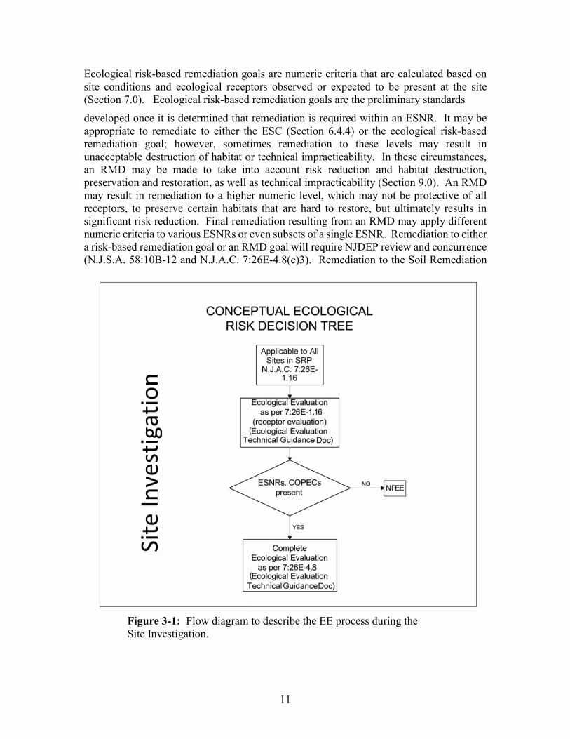
The guidance first describes how to conduct an EE, which is initiated during the Site Investigation (SI) pursuant to N.J.A.C. 7:26E-1.16. The EE is conducted to examine the site for the co-occurrence of the following:
(1) ESNRs on, adjacent to, or potentially impacted by the site; (2) the presence of Contaminants of Potential Ecological Concern (COPEC) at the site
or area of concern (AOC) and in the ESNRs (e.g., contaminants with concentrations in excess of aquatic Surface Water Quality Standards (SWQS) or ecological screening criteria (ESC)); and
(3) the presence of a contaminant migration pathway (historic or current) from the site to the ESNR or evidence of contaminated material having been placed directly into an ESNR. As part of the SI, an EE must be performed within the regulatory time frame of one year from the initiation of remediation (N.J.A.C. 7:26C-3.2). The mandatory time frame associated with this requirement is two years from the initiation of remediation (N.J.A.C. 7:26C-3.3). The outcome of the EE will be a recommendation either to conduct an ERA or to not conduct any further ecological evaluation.
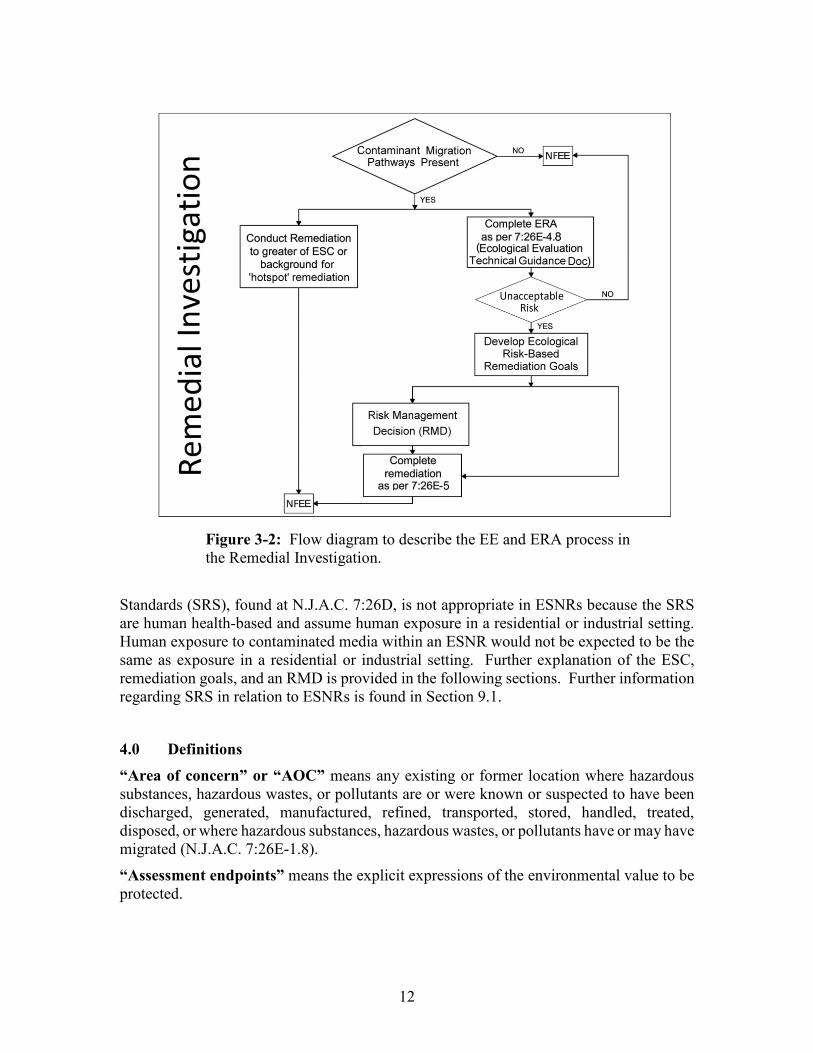
Guidance is then provided on how to conduct the ERA, a component of the Remedial Investigation (RI) pursuant to N.J.A.C. 7:26E-4.8. The ERA is a quantitative assessment of the actual or potential impacts of COPECs from a contaminated site on ecological receptors associated with ESNRs on, adjacent to or potentially impacted by the site. The ERA will do the following:
(1) determine whether actual or potential ecological risks exist at a site based on rigorous site-specific biological tests;
(2) identify whether remediation is necessary for those constituents posing ecological risks; and
(3) generate data needed to determine site-specific ecological risk-based remediation goals and RMDs.
An overview of the EE and ERA process is provided in Figures 3-1 and 3.2 below.
While conducting an EE and ERA, the numeric criteria potentially used to evaluate contaminant levels associated with ESNRs include ESC, calculated ecological risk-based remediation goals, and RMD goals. ESC are literature values for individual contaminants that are conservative screening values intended to be protective of the target organisms based on direct exposure. The ESC are used in the initial stages of the EE to determine whether there is potential for site contaminants to impact ESNRs (Section 5.4). If site contaminant levels are less than or equal to the ESC for all samples, then no further ecological evaluation may be appropriate; however, if any of the site contaminants are above the ESC, then further evaluation will be required (Section 5.5). Contaminants without ESCs must be evaluated in the risk assessment process (N.J.S.A. 58:10B-12).
11
Ecological risk-based remediation goals are numeric criteria that are calculated based on site conditions and ecological receptors observed or expected to be present at the site (Section 7.0). Ecological risk-based remediation goals are the preliminary standards
developed once it is determined that remediation is required within an ESNR. It may be appropriate to remediate to either the ESC (Section 6.4.4) or the ecological risk-based remediation goal; however, sometimes remediation to these levels may result in unacceptable destruction of habitat or technical impracticability. In these circumstances, an RMD may be made to take into account risk reduction and habitat destruction, preservation and restoration, as well as technical impracticability (Section 9.0). An RMD may result in remediation to a higher numeric level, which may not be protective of all receptors, to preserve certain habitats that are hard to restore, but ultimately results in significant risk reduction. Final remediation resulting from an RMD may apply different numeric criteria to various ESNRs or even subsets of a single ESNR. Remediation to either a risk-based remediation goal or an RMD goal will require NJDEP review and concurrence (N.J.S.A. 58:10B-12 and N.J.A.C. 7:26E-4.8(c)3). Remediation to the Soil Remediation
Figure 3-1: Flow diagram to describe the EE process during the Site Investigation.
12
Standards (SRS), found at N.J.A.C. 7:26D, is not appropriate in ESNRs because the SRS are human health-based and assume human exposure in a residential or industrial setting. Human exposure to contaminated media within an ESNR would not be expected to be the same as exposure in a residential or industrial setting. Further explanation of the ESC, remediation goals, and an RMD is provided in the following sections. Further information regarding SRS in relation to ESNRs is found in Section 9.1. 4.0 Definitions “Area of concern” or “AOC” means any existing or former location where hazardous substances, hazardous wastes, or pollutants are or were known or suspected to have been discharged, generated, manufactured, refined, transported, stored, handled, treated, disposed, or where hazardous substances, hazardous wastes, or pollutants have or may have migrated (N.J.A.C. 7:26E-1.8).
“Assessment endpoints” means the explicit expressions of the environmental value to be protected.
Figure 3-2: Flow diagram to describe the EE and ERA process in the Remedial Investigation.
13
“Background Area” means an area as close to the site as possible, with a habitat similar to the habitat being assessed in terms of physical, geochemical, and biological characteristics, but one that is outside of the influence of the site discharge.
“Background Contamination” means the contaminant concentrations in all media for which remediation goals have been or will be established, e.g., abiotic media (soil, sediment, surface water) and biological tissues. The Background contamination should not be attributable to the site discharge itself, but may have originated from either natural sources (not man-made) or anthropogenic sources (offsite discharges from diffuse anthropogenic or other unavoidable discharges, such as permitted wastewater discharges/CSOs or storm water). These background contaminant concentrations are generally derived by collecting samples in the background area. Background data should not be collected from areas influenced by other contaminated sites or locations in the immediate vicinity of point or non-point source outfalls, tributary confluences, road/bridge runoff, etc., since localized elevated contaminant concentrations or hot spots may be present and would not be representative of the background area contaminant levels.
“Benthic community” means organisms that live in and on the bottom substrate of a surface water body.
“Benthic macroinvertebrate survey” means the use of macroinvertebrate collection, organism identification, and data analysis to assess various metrics including community, population, and functional parameters such as species richness and tolerance indices.
“Bioaccumulation” means the accumulation of contaminants in the tissue of organisms through any route, including respiration, ingestion, or direct contact with contaminated media (USEPA 2000c).
“Bioavailability” means the individual physical, chemical, and biological interactions that determine the exposure of plants and animals to chemicals associated with soils and sediments (ITRC 2011).
“Biomagnification” means the process of bioconcentration and bioaccumulation by which tissue concentrations of bioaccumulated chemicals increase as the chemical passes up through two or more trophic levels. The term implies an efficient transfer of chemical from food to consumer, so that residue concentrations increase systematically from one trophic level to the next (USEPA 2000c).
“Biotic Zone” means the interval in soil/sediment that corresponds to the highest level of biological activity. In terrestrial soil, biological activity is typically associated with soil invertebrates, plant/root production, and microorganisms; while in sediment the activity is associated with the macroinvertebrate community. This zone is generally related to the 0-6” interval for sediments and generally 0-12” for soils, however, it may extend to deeper intervals in certain habitat settings or when burrowing receptors are present. While the NJDEP acknowledges that the depth of the biotic zone may vary, in accordance with Section 3.3 of the Technical Guidance for Site Investigation of Soil, Remedial Investigation of Soil, and Remedial Action Verification Sampling for Soil, samples should be collected from discrete 6-inch intervals.
“Breeding season” means the most suitable season, usually with favorable conditions and abundant food and water, for breeding among some wild animals and birds (wildlife).
14
“Chlorotic vegetation” means the abnormally yellowing or whitening of normally green plant tissue, resulting from partial failure to develop chlorophyll or decreased production of chlorophyll.
“Comingled contamination” means unrelated contaminants that are mixed in an area or media.
“Community assessment” means the evaluation of community structure by measuring biotic characteristics (e.g., species abundance, diversity, and composition); community assessment may also include evaluating community function by measuring rate processes (e.g., species colonization rates).
“Congener” means any of the 75 isomers of dioxin, 135 isomers of furans and 209 isomers of PCBs that differ in the number and position of chlorine atoms attached to the base structure of the molecule. There are 7 dioxin congeners, 10 furan congeners and 12 PCB congeners that the World Health Organization (WHO) has identified as having dioxin-like properties.
“Contaminant delineation” means the determination of the vertical and horizontal extent of contamination in all surface water, sediment, and soils within environmentally sensitive natural resources to the higher of the ecological screening criteria or background contaminant levels, or risk-based remediation goals.
“Contaminant migration pathway” means the potential conduit for movement of contaminants from one area or media to another via a route or way of access.
“Contaminant of Potential Ecological Concern” or “COPEC” means a substance detected at a contaminated site that has the potential to adversely affect ecological receptors because of its concentration, distribution, and mode of toxicity; contaminants with concentrations above their respective New Jersey Surface Water Quality Standards or ecological screening criteria are identified as contaminants of potential ecological concern.
“Contaminated site” means all portions of environmental media at a site and any location where contamination is emanating, or which has emanated, therefrom, that contain one or more contaminants at a concentration which fails to satisfy any applicable remediation standard (N.J.A.C. 7:26E-1.8).
“Contamination” or “contaminant” means any discharged hazardous substance as defined pursuant to N.J.S.A. 58:10-23.11b, hazardous waste as defined pursuant to N.J.S.A. 13:1E-38, or pollutant as defined pursuant to N.J.S.A. 58:10A-3 (N.J.A.C. 7:26E-1.8).
“Data quality objectives” means performance and acceptance criteria that clarify study objectives, define the appropriate type of data, and specify tolerable levels of potential decision errors that will be used as the basis for establishing the quality and quantity of data needed to support decisions.
“Dredged materials” means subaqueous media moved within or removed from a given water body by deliberate action via mechanical or hydraulic means.
“Ecological Conceptual Site Model” or “ECSM” means the conceptual projection of possible source-to-pathway-to-receptor scenarios for the COPECs identified at a site.
15
“Ecological Evaluation” means the process by which each contaminated site or AOC is investigated for the co-occurrence of ESNRs, COPECs, and contaminant migration pathways from the source area to the ESNR.
“Ecological Risk Assessment” means a qualitative or quantitative appraisal of the actual or potential impacts of contaminants from a contaminated site on plants and animals other than humans and domesticated species.
“Ecological risk-based remediation goal” means risk-based numeric criteria that are calculated based on site conditions and ecological receptors observed or expected to be present at the site. Remediation goals are the preliminary standards developed once it is determined that remediation is required within an ESNR.
“Ecological screening criteria” or “ESC” means literature values for individual contaminants that were usually derived by dosing experiments and that are mainly based on the no observed adverse effect level (NOAEL) or lowest observed adverse effect level (LOAEL). The ESC are generally conservative levels designed to protect the target organisms based on direct exposure.
“Ecotoxicological effect” means any adverse acute or chronic effect from contaminants on invertebrate, plant, fish or wildlife individual, population, or community.
“Endangered Species” means a plant or animal species whose prospects for survival within the state are in immediate danger because of one or several factors such as loss or degradation of habitat, overexploitation, predation, competition, disease or environmental pollution, etc. An endangered species likely requires immediate action to avoid extinction within New Jersey.
“Environmental medium” means any component such as soil, air, sediment, structures, ground water or surface water (N.J.A.C. 7:26E-1.8).
“Environmentally sensitive natural resources” means any area that supports any wildlife including all areas defined at N.J.A.C. 7:1E-1.8(a), ground water, and areas and/or resources that are protected or managed pursuant to the Pinelands Protection Act, N.J.S.A. 13:18A-1 et seq. and the Pinelands Comprehensive Management Plan, N.J.A.C. 7:50 (N.J.A.C. 7:26E-1.8).
“Epibenthic” means living and feeding on top of the sediment, but may be hidden by leaves and organic detritus.
“Estuary” means a tidally influenced area where freshwater inputs from rivers, streams or other conveyances enter coastal marine environments.
“Fecundity” means the capacity, especially in female animals, of producing young in abundance.
“Feeding guild” means a group of unrelated species that feed on similar foods (e.g., benthivore, detritivore, herbivore, insectivore, omnivore, planktivore, piscivore), or the types of food that an individual organism feeds upon.
“Fresh water(s)” means all nontidal and tidal waters generally having a salinity, due to natural sources, of less than or equal to 3.5 parts per thousand at mean high tide (N.J.A.C. 7:9B-1.4).
16
“Geographic Information System” means a computer system for capturing, storing, checking, integrating, manipulating, analyzing, and displaying data related to positions on the earth's surface.
“Ground water” means the portion of the water beneath the land surface that is within the zone of saturation where all pore spaces of the geologic formation are filled with water (N.J.A.C. 7:26E-1.8).
“Hazard quotient” or “HQ” means the ratio of the results of the measured or modeled dietary contaminant doses to receptors of concern to the toxicity reference value.
“Historic fill material” means non-indigenous material, deposited to raise the topographic elevation of the site, which was contaminated prior to emplacement, and is in no way connected with the operations at the location of emplacement and which includes, without limitation, construction debris, dredge materials, incinerator residue, demolition debris, fly ash, or non-hazardous solid waste. Historic fill material does not include any material which is substantially chromate chemical production waste or any other chemical production waste or waste from processing of metal or mineral ores, residues, slag or tailings. In addition, historic fill material does not include a municipal solid waste landfill site (N.J.A.C. 7:26E-1.8).
“Homolog” means one of a series of congeners with the same number of chlorine atoms.
“Inhibitory concentration” or “IC” means the test concentration that yielded an inhibitory effect on a given percentage of the exposed organisms.
“Lentic” means the ecosystem of a lake, pond or swamp.
“Lotic” means the ecosystem of a river, stream or spring.
“Lowest observed adverse effects level” or “LOAEL” means the lowest level of exposure of an organism, found by experiment or observation, at which there is a biologically or statistically significant increase in the frequency or severity of any adverse effects in the exposed population when compared to its appropriate control.
“Lowest observed effect concentration” or “LOEC” means the lowest test concentration at which a significant reduction in survival, growth, or reproduction/fecundity as compared to the laboratory control or reference sample was observed.
“Measurement endpoint” means a measurable response to a stressor that is related to the valued characteristic chosen as the assessment endpoint.
“Method detections limit” or “MDL” means the minimum concentration of a substance that can be measured and reported with a 99 percent confidence that the analyte concentration is greater than zero and is determined from the analysis of a sample in a given matrix containing the analyte (N.J.A.C. 7:26E-1.8).
“Mixing zone” means the area of a tidal water body of a site or contaminant source where the tidal action is capable of transporting sediment or contaminants within that reach.
“No observed adverse effect level” or “NOAEL” means the level of exposure of an organism, found by experiment or observation, at which there is no biologically or statistically significant increase in the frequency or severity of any adverse effects in the exposed population when compared to its appropriate control.
17
“No observed effect concentration” or “NOEC” means the highest test concentration at which there is no statistically significant reduction in survival, growth, or reproduction/fecundity as compared to the laboratory control or reference sample.
“Non-targeted compound” means a compound detected in a sample using a specific analytical method that is not a targeted compound, a surrogate compound, a system monitoring compound or an internal standard compound (N.J.A.C. 7:26E-1.8).
“Parthenogenic” means that the unfertilized egg of a female of a given species develops into a new individual of that species and does not require a male to fertilize the eggs for reproduction.
“Pinelands” means any area consistent with the provisions of the Pinelands Protection Act, N.J.S.A. 13:18A-1 et seq. and any rules promulgated pursuant thereto, and with section 502 of the National Parks and Recreation Act of 1978, 16 U.S.C. §4711.
“Rare Species” means a group of organisms that is very uncommon or scarce. This designation may be applied to either a plant or animal taxon, and may be distinct from the term “endangered" or “threatened species."
“Receptor” means any human or other ecological component that is or may be affected by a contaminant from a contaminated site (N.J.A.C. 7:26E-1.8).
“Receptor Evaluation” means the general and reporting requirements specified in N.J.A.C.7:26E -1.12 through 1.16.
“Receptor Evaluation form” means the form required by the NJDEP pursuant to N.J.A.C. 7:26E -1.12(c) and (e).
“Reference Area” means an area as uncontaminated as possible that may or may not be within the background area and may or may not be in close proximity to the site. The reference area must not be influenced by the site discharge itself or from regulated contaminated sites slated for remedial investigation or remedial action, and should only be influenced by natural sources (not man-made) or unavoidable diffuse anthropogenic sources. The samples should not be collected from locations directly influenced by or in proximity to other obvious sources of contamination (e.g., other contaminated sites, sewer and storm-water outfalls, tributaries, and other point and nonpoint source discharges). The reference area must have a habitat similar to the habitat being assessed in terms of physical, geochemical, and biological characteristics.
“Reference and biological reference data” means the contaminant concentrations for abiotic media (soil, sediment, surface water) and biological tissue, as well as data from sediment/soil toxicity tests and fish/benthic macroinvertebrate/soil invertebrate community surveys.
“Remediation standards” means the combination of numeric standards that establish a level or concentration, and narrative standards, to which contaminants must be treated, removed or otherwise cleaned for soil, ground water or surface water, as provided by the NJDEP pursuant to N.J.S.A. 58:10B-12, in order to meet the health risk or environmental standards (N.J.A.C. 7:26E-1.8).
“Riparian” means of, pertaining to, or situated or dwelling on the bank of a river or other body of water.
18
“Risk management strategy” or “risk management decision” or “RMD” means a decision to remediate an ESNR to a level other than the calculated ecological risk-based remediation goal by taking into account risk reduction, habitat destruction, preservation and restoration, and technical impracticability. A risk management decision may result in remediation to a higher numeric level, which may not be protective of all receptors, to preserve certain habitats that are hard to restore but ultimately results in significant risk reduction.
“Saline waters” means waters having salinities generally greater than 3.5 parts per thousand at mean high tide (N.J.A.C. 7:9B-1.4).
“Sediment” means unconsolidated material (particles including gravel, sand, silt, clay and other natural and anthropogenic substances) that has been deposited from water and settles to the bottom of a surface water body or within a wetland, and contains porewater. All unconsolidated material below a waterbody is considered sediment for the purpose of remedial investigations and remedial actions (for additional information see Section 5.4.3)
“Sediment pore water” means the water located in the interstitial space between the sediment solid-phase particles.
“Sediment quality triad approach” means the use of benthic macroinvertebrate surveys, sediment chemistry and sediment toxicity tests to provide a measure of ecosystem health.
“Site investigation” means the collection and evaluation of data adequate to determine whether or not discharged contaminants exist at a site or have migrated or are migrating from the site at levels in excess of the applicable remediation standards. A site investigation shall be developed based upon the information collected pursuant to the preliminary assessment. The requirements of a site investigation are set forth at N.J.A.C. 7:26E-3 (N.J.A.C. 7:26E-1.8).
“Surface water” means water defined as surface water pursuant to the Surface Water Quality Regulations, N.J.A.C. 7:9B (N.J.A.C. 7:26E-1.8).
“Taxonomic class” means the group an organism is placed into by the orderly classification of plants and animals according to their presumed natural relationships based on similarities of structure, origin, etc.
“Technical Impracticability” means a condition where remediation to the applicable NJDEP standards is not feasible from an engineering perspective if: current engineering methods or best available technologies designed to meet the applicable standards cannot be reasonably implemented. TI determinations can be applied to an entire site or a portion thereof. The TI determination does not relieve the responsible party of their ultimate responsibility of achieving applicable NJDEP standards. If such a determination is made, but subsequent advances in remedial technologies or changes in site conditions make achievement of the standards practicable, NJDEP reserves the authority to modify the TI determination, as appropriate. Impracticability does not equate to “no action.” When a remedial action is deemed impractical, the remediating party must put in place other measures to safeguard potential receptors in accordance with N.J.A.C. 7:26E-5.1(e). (NJDEP Technical Impracticability Guidance for Groundwater Document).
“Tentatively identified compound” or “TIC” means a non-targeted compound detected in a sample using a GC/MS analytical method which has been tentatively identified using
19
a mass spectral library search. An estimated concentration of the TIC is also determined (N.J.A.C. 7:26E-1.8).
“Threatened species” means a species that may become endangered if conditions surrounding it begin to or continue to deteriorate. Thus, a threatened species is one that is already vulnerable as a result of, for example, small population size, restricted range, narrow habitat affinities, significant population decline, etc.
“Toxicity reference value” or “TRV” means a dose above which ecologically relevant effects might occur to wildlife species following chronic dietary exposure and below which it is reasonably expected that such effects will not occur.
“Wetlands” means those areas that are inundated or saturated by surface or groundwater at a frequency or duration sufficient to support, and that under normal circumstances does support, a prevalence of vegetation typically adapted for life in saturated soil conditions. Wetlands generally include swamps, marshes, bogs, and similar areas (40 CFR 230.3).
5.0 Technical Guidance for Preparing Ecological Evaluations The purpose of the EE is to assess actual or potential adverse ecological effects on wildlife and plants in ESNRs resulting from site-related contamination and in certain circumstances other contamination not related to the site such as historic fill material and dredged materials (Section 6.4.8). During the EE, the site is examined for the co-occurrence of the following:
(1) ESNRs on, adjacent to, or potentially impacted by the site; (2) the presence of COPECs at the site or AOC and in the ESNRs; and (3) the presence of a contaminant migration pathway from the site to the ESNR, or
evidence of contaminated material having been placed directly into an ESNR.
The outcome of the EE will be a recommendation either to conduct an ERA or to not conduct further ecological evaluation. The investigator must be experienced in the use of techniques and methodologies for conducting ERAs in accordance with appropriate USEPA guidance, which includes, but is not limited to ERAGS (N.J.S.A. 58:10C-16(c)).
The EE is an iterative process beginning with the EE that is conducted pursuant to N.J.A.C. 7:26E-1.16, and finishing with conclusions regarding the need for an ERA conducted pursuant to N.J.A.C. 7:26E-4.8.
5.1 Ecological Evaluation Pursuant to N.J.A.C. 7:26E-1.16 Pursuant to N.J.A.C. 7:26E-1.16 and in accordance with Section 5.2, an EE must be initiated in the SI phase with the initial results of the EE submitted as part of the Receptor Evaluation Form and supporting documentation pursuant to N.J.A.C. 7:26E-1.16. The EE documents the following:
(1) whether ESNRs are present on or adjacent to the site or are in locations receiving discharges from the site;
(2) a preliminary identification of whether the site contains any contaminants above ESCs (based upon existing data if available); and
(3) an initial assessment of possible contaminant migration pathways.
20
Much of this stage of the EE process can be completed using desk-top information, although a qualitative field survey should be conducted to verify the presence of ESNRs.
5.2 Ecological Evaluation Pursuant to N.J.A.C. 7:26E-4.8 Under N.J.A.C. 7:26E-1.16, the first two steps of the Ecological Evaluation (EE) are conducted to verify the presence of ESNRs and COPECs (above ESCs at the AOC or ESNR). After this stage, if ESNRs and COPECs are present, then pursuant to N.J.A.C. 7:26E-4.8(a) and (b), sampling within the potential migration pathway and ESNR to support the EE may be conducted during the RI. At a minimum, the investigator must determine whether contaminant concentrations are present at the AOC in excess of ESCs or SWQS (N.J.A.C. 7:26E-1.16). Supplemental sampling specific to that ESNR may be warranted to determine whether COPECs in excess of ESCs are present in the ESNR. The investigator may decide that food chain modeling is appropriate as part of the completion of the EE. If food chain modeling will be conducted as part of the EE, the modeling should use conservative input parameters as specified in ERAGS (i.e., area use factor of 1 and maximum soil/sediment concentration). Detailed procedures for conducting food chain analysis can be found in Section 6.1.3.1.
Guidance for the identification and sampling of ESNRs, COPECs, and contaminant migration pathways is provided below.
5.2.1 Environmentally Sensitive Natural Resources Pursuant to N.J.A.C. 7:26E-1.16, the investigator must identify whether ESNRs are present on the site or area of concern, adjacent to the site or area of concern, or may be, have been, or are impacted by contamination from the site or area of Concern. ESNRs are habitats where concern for plant and wildlife exposure to site COPECs is paramount. Man-made features, such as ditches, waste lagoons, and impoundments should be evaluated to determine whether they function as ESNRs or they discharge to an ESNR. Use the following information sources to identify ESNRs: • NJDEP’s NJ-GeoWeb, available with user guidance at
http://www.nj.gov/dep/gis/geowebsplash.htm with links to Internet mapping applications;
• NJDEP’s “Landscape Project” with data downloads available at http://www.state.nj.us/dep/fgw/ensp/landscape;
• NJ Natural Heritage Program, information on rare, threatened and endangered species, http://www.state.nj.us/dep/parksandforests/natural/heritage
A qualitative habitat or vegetative community survey should be performed to provide a general description of land use, to identify the ESNRs present at the site, and to confirm the information obtained from the NJDEP’s Geographic Information System (GIS). The investigator should be familiar with state and federal guidance and literature references for plant community assessment, such as the Federal Manual for Identifying and Delineating Jurisdictional Wetlands (Federal Interagency Committee for Wetland Delineation, 1989). The dominant plant species for each vegetative stratum (e.g., canopy, shrub, vine, and herbaceous layer)
21
should be visually estimated as per standard procedure. The qualitative survey should be conducted during the prime growing season if possible (May to September) to assess indicators of stressed vegetation, such as stunted growth, chlorosis, brown or drying leaf tips, barren soil. Absence of stressed vegetation does not mean absence of contamination or impact.
The investigator should document biota observed or expected to use or inhabit each ESNR for any period of time, whether year-round or during the breeding, foraging, resting, migration or wintering seasons. Wildlife should be identified by taxonomic class, common and scientific names, feeding guild, and location of residence among the habitat types. Wildlife should be identified based on actual sightings or evidence (e.g., tracks, scat, nests, song, and call). Expected wildlife should be based on literature reviews or professional judgment.
A formal wetland delineation or functional assessment may be appropriate on a site-specific basis in accordance with the New Jersey Freshwater Protection Act Rules, N.J.A.C.7:26A. See Section 6.4.1 for additional information.
If ESNRs do not exist, it is not necessary to complete the requirements of Sections 5.2 through 5.4, and documentation of the lack of ESNRs should comprise the EE report. If ESNRs exist, complete Sections 5.2 through 5.5.
The EE submitted as part of the Receptor Evaluation should document the presence of ESNRs on-site, adjacent to the site, or in areas potentially receiving contaminants from the site. The location of ESNRs should be presented diagrammatically using maps and figures showing the site. Stream classification and antidegradation designation should be documented.
5.2.2 Contaminants of Potential Ecological Concern Pursuant to N.J.A.C. 7:26E-1.16(b) and 4.8(c), the investigator must identify the presence of Contaminants of Potential Environmental Concern (COPEC). Compare all surface water, sediment, soil, and groundwater (from monitoring wells or piezometers proximal to ESNRs) data collected from contaminant migration pathways and ESNRs to ESCs and standards in the most recent version of the NJDEP Ecological Screening Criteria Table, available at http://www.nj.gov/dep/srp/guidance/ecoscreening/ (Section 5.4). At a minimum, those contaminants that exceed the ESC or standards or do not have an ESC should be considered COPECs.
If all ESNR contaminant concentrations are less than the ecological screening criteria, and contaminants without ecological screening criteria are not present, then further ecological investigation is not required.
If any ESNR contaminant concentrations exceed ecological screening criteria, or contaminants without ecological screening criteria are present, then further ecological investigation is required. Tentatively identified compounds (TICs) must be addressed pursuant to N.J.A.C. 7:26E-2.1(e). Further investigation of TICs may include a statistical summary (i.e. frequency of detection, range of detection, etc.), comparison with background data, use of specialty analytical services, or site-specific testing such as toxicity testing to determine whether the TIC constitutes a
22
COPEC. TICs which are frequently detected or are detected at high concentrations should be carried forward in the ERA process.
The investigator should ensure that the laboratory meets the method detection limits (MDL) as specified by the analytical method and should highlight where the sample analytical detection limits exceed the ESC and standards for the site COPECs. For the initial screening, it is standard practice for the investigator to use one half of the MDL for comparison to ESCs in those circumstances where the detection limit exceeds the ESC and the analytical result is nondetect.
5.2.3 Contaminant Migration Pathways Pursuant to N.J.A.C. 7:26E-4.8(a) and (b), the investigator must identify current and historic actual and potential contaminant migration pathways to ESNRs, including the possibility that direct dumping or discharge may be occurring or may have occurred historically (possibly before site records document otherwise). The investigator should evaluate site topography, contaminant chemical characteristics, fate and transport mechanisms, and site features or practices that may facilitate or have facilitated contaminant migration. Current and historic presence of surface or subsurface piping beds, drains, ditches, lagoons, and locations where current or historic direct discharges could have occurred, such as from over-water or over-shoreline product transfers, dumping from trucks, etc., should be considered.
The investigator should identify direct evidence of contaminant migration by visual indicators. Examples of direct observations of contaminant migration include, but are not limited to, stressed, stunted, chlorotic, and dead vegetation, discolored soil, sediment, or water, acute effects on biota, absence of biota (plants and animals) in a specified area of the ESNR that would be expected as compared to a similar unimpacted ESNR, presence of seeps, sheens, discharges, and evidence of surface erosion.
The investigator should identify potential contaminant migration pathways. Such pathways may include, but are not limited to, contaminant migration during storm events, tidal reversals, discharge of contaminated groundwater to surface water, food chain transfer, and the potential for direct disposal or discharge of site COPECs to ESNRs. An example of potential migration is where a riparian area or floodplain surrounding a contaminated surface water body may become contaminated during flood events.
The investigator should ensure that all contaminant migration pathways have been considered in the sampling plan design and data have been collected in appropriate ESNRs. Data gaps should be identified in the EE report (Section 5.5(b)ii).
5.3 Recommended Sample Collection in Support of Ecological Evaluations Generally, the goals of a surface water, sediment or soil sampling program include preliminary and definitive determination of the nature and areal extent of contamination and identification of areas of highest contamination. Data are also to be gathered in support of ERAs, long-term monitoring, or for sediment transport and deposition modeling or contaminant migration or natural attenuation. The surface water, sediment or soil sampling plan must be a component of the SI or RI Work Plan, and must be
23
prepared pursuant to N.J.A.C. 7:26E and the NJDEP Field Sampling Procedures Manual (FSPM) (NJDEP, August 2005 or most recent version at http://www.state.nj.us/dep/srp/guidance/fspm/). Site-specific details regarding the study objectives, data quality objectives (DQO), sampling methodology, location, and depth of samples must be specified, as well as field and laboratory quality assurance and quality control (QA/QC) procedures (N.J.A.C. 7:26E). Guidance and special considerations for designing a surface water, sediment, and soil sampling scheme are provided herein to supplement and highlight the regulatory requirements and FSPM guidance; the reader is referred to these documents for a comprehensive treatment of the subject. The reader is referred to USEPA’s Sediment Sampling Quality Assurance User’s Guide (USEPA, 1985a), Methods for Collection, Storage and Manipulation of Sediments for Chemical and Toxicological Analyses: Technical Manual (USEPA, 2001) and the FSPM (NJDEP, 2005) for guidance on statistically determining the appropriate number of samples.
5.3.1 When to Collect Samples When contaminants are found in on-site media in excess of the ESC and ESNRs are on, adjacent to or potentially impacted by the site, as defined at N.J.A.C. 7:26E-1.8, environmental samples are to be collected in the potential migration pathways and in the ESNRs, as appropriate. N.J.A.C. 7:26E-1.8 defines contaminated sites as all portions of environmental media at a site and any location where contamination is emanating, or which has emanated, therefrom, that contain one or more contaminants at a concentration which fails to satisfy any applicable remediation standard. If the investigator can provide documentation that site-related contamination in surface water, sediment, wetlands, or soil in ESNRs is unlikely, based on site-specific conditions, site history, etc., then additional sampling of ESNR or contaminant migration pathways may not be required, refer to Figure 3-1.
Samples should be collected in ESNRs and contaminant migration pathways under any of the following conditions:
(1) if known historical discharges have occurred or on-going discharges are occurring, as determined pursuant to Section 5.2.3;
(2) if there is a presence of stressed vegetation, sheens, seeps, discolored soil or sediment along the shoreline or on the surface water body or wetland;
(3) if there is evidence of stream impacts from historical discharges including historical ecological studies documenting differences in organism population density and diversity in areas potentially impacted by the site relative to areas not impacted by the site; or
(4) if there is a groundwater discharge to surface water or a wetland, with contaminants originating on site above the applicable SWQS or ESC.
Sampling must be designed to account for seasonal or short-term flow and water quality fluctuations caused by dry- versus wet-weather flow, system hydraulics (obtaining flow-proportioned samples where applicable), and potential contaminant characteristics (e.g., density and solubility) (N.J.A.C. 7:26E-3.6(b)). In addition to other required analyses, sediments must also be analyzed for total organic carbon
24
(TOC), pH, and particle size (N.J.A.C. 7:26E-3.6(b)). These data are required to develop appropriate remediation standards. Depending on the type of contaminant, type of discharge (e.g., surficial and subsurface), and media potentially impacted, the sampling methods and depth will vary as indicated below.
5.3.2 Where to Collect Samples The following sections provide general and media-specific guidance for the selection of sampling locations.
5.3.2.1 Potential Contaminant Migration Pathways I. Ditches and Swales
Ditches and swales that do not contain standing or flowing water should be sampled as indicated in Section 5.3.2.2 II or III. Ditches and swales that contain standing water should be sampled as indicated in Section 5.3.2.2 I. A. Ditches and swales that contain flowing water should be sampled as indicated in Section 5.3.2.2 I. B.
II. Overland Flow
When the potential migration pathway consists of general overland flow with no discernable ditches or swales, samples should be collected as indicated in Section 5.3.2.2 III.
III. Groundwater
When the potential migration pathway consists of groundwater, samples should be collected in accordance with N.J.A.C. 7:26E-3.5, Site investigation-groundwater, and the relevant technical guidance. Samples from the most downgradient monitoring wells or piezometers, or samples in the closest proximity to ESNRs will be considered indicative of the migration pathway.
5.3.2.2 Environmentally Sensitive Natural Resources I. Aquatic Systems
In aquatic systems, the areas of greatest contamination will generally occur in depositional areas, thus these should be specifically targeted by the sampling plan. Such depositional areas are generally characterized by slow-moving water where fine sediments tend to accumulate (e.g., pool areas, river bends). Sediment samples collected for chemical analysis, toxicity testing, and benthic community surveys should be spatially and temporally collocated. Sediment samples should be collected in a manner to avoid the loss of fine-grained sediments. Surface water and sediment samples should be spatially and temporally collocated. Surface water samples should be collected before sediment samples to avoid suspended sediments in surface-water samples. Samples should be collected in downstream areas first, and then successively at upstream sampling locations.
A. Standing water areas (e.g., ponds, lakes, wetlands, surface impoundments, lagoons, storm water detention ponds, fire ponds, and excavations, natural
25
depressions and diked areas that can accumulate water) should be sampled as follows:
1. Collect a minimum of three surface water samples and three sediment samples in each area where there is evidence of a historical or ongoing discharge, including but not limited to, stressed vegetation, sheens, seeps, discolored soil or sediment along the shoreline or in a wetland, or other evidence of a discharge;
2. Collect a minimum of one surface water and sediment sample at each inflow and outflow area; and
3. Collect a minimum of one surface water and sediment sample at each depositional area where sediments may be expected to accumulate.
B. Flowing water areas (e.g., rivers, streams, creeks, wetlands, culverts, and swales) should be sampled as follows: Collect a minimum of one sediment sample where sediments are expected to accumulate and a minimum of one surface-water sample under low flow (base flow) and high flow conditions as follows:
1. Collect a minimum of one surface-water and one sediment sample up stream of the point or area of discharge;
2. Collect a minimum of one surface-water and one sediment sample downstream of the point or area of discharge; and
3. Collect a minimum of one surface-water and one sediment sample at the point or area of discharge.
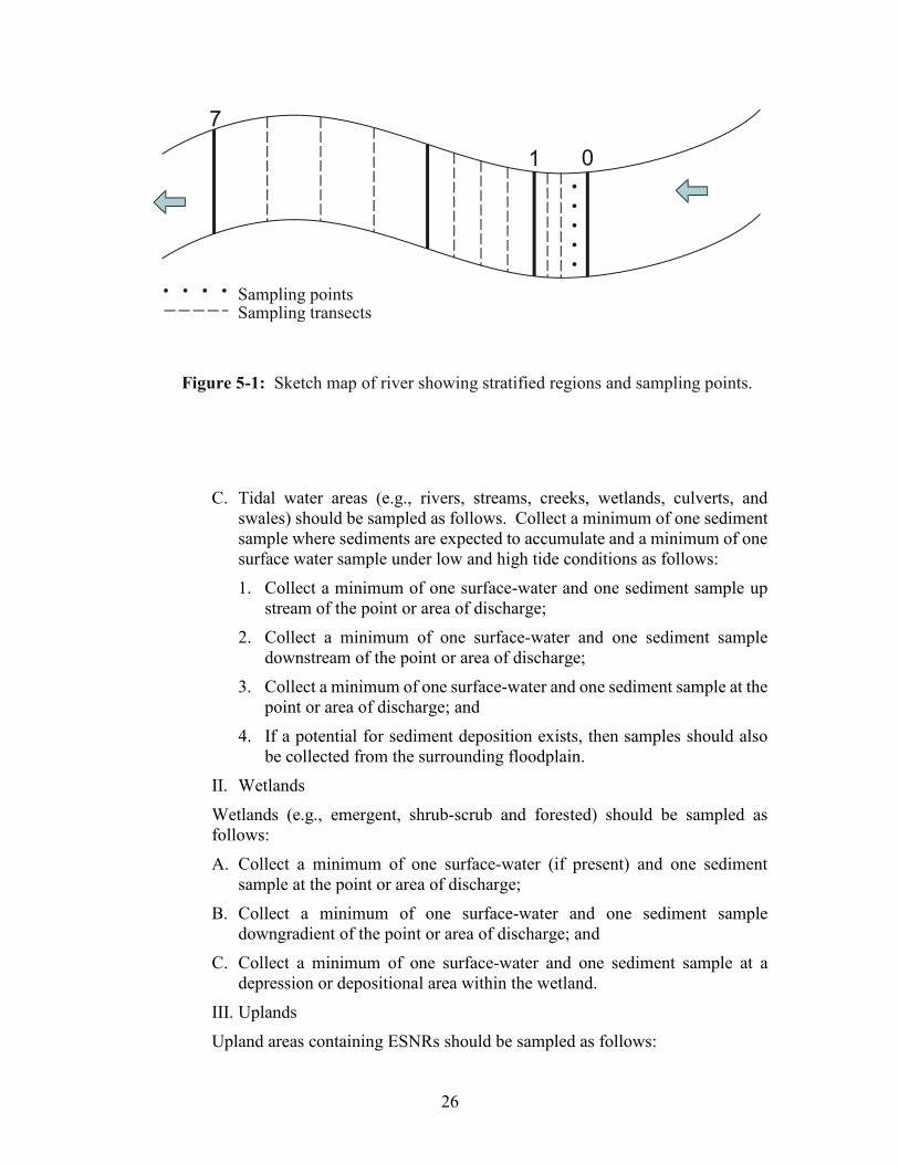
A commonly used approach to locating sediment samples is as follows: The stream location adjacent to the contaminated site most likely to receive contaminant input via the contaminant migration pathway is considered the initial sample point. The study region is divided into linear segments and sample transects are located systematically within each segment; the length of the segments and distance between transects increases with increasing distance downstream. This approach is depicted in Figure 5-1, a diagram of a sampling plan indicating 15 sediment samples per segment region. In this example, the first segment is from zero to one km, the second from one to three km, and third from three to seven km. The sampling transects (indicated by dashed lines) are located at 1/4, 1/2, and 3/4 the distance along each segment. Sample points (indicated by five dots) are located along the transects at 1/6, 1/3, 1/2, 2/3, and 5/6 the distance bank to bank (USEPA, 1985a). The distance from bank to bank is measured from the mean high-water mark.
If a potential for sediment deposition exists, then samples should also be collected from the surrounding floodplain. The actual number and location of sample points will be decided on a case-by-case basis, based on the study objectives, water-body dimensions, flow conditions, substrate conditions, availability of previous data, etc.
26
C. Tidal water areas (e.g., rivers, streams, creeks, wetlands, culverts, and swales) should be sampled as follows. Collect a minimum of one sediment sample where sediments are expected to accumulate and a minimum of one surface water sample under low and high tide conditions as follows:
1. Collect a minimum of one surface-water and one sediment sample up stream of the point or area of discharge;
2. Collect a minimum of one surface-water and one sediment sample downstream of the point or area of discharge;
3. Collect a minimum of one surface-water and one sediment sample at the point or area of discharge; and
4. If a potential for sediment deposition exists, then samples should also be collected from the surrounding floodplain.
II. Wetlands
Wetlands (e.g., emergent, shrub-scrub and forested) should be sampled as follows:
A. Collect a minimum of one surface-water (if present) and one sediment sample at the point or area of discharge;
B. Collect a minimum of one surface-water and one sediment sample downgradient of the point or area of discharge; and
C. Collect a minimum of one surface-water and one sediment sample at a depression or depositional area within the wetland.
III. Uplands
Upland areas containing ESNRs should be sampled as follows:
7
1 0
Sampling points Sampling transects
Figure 5-1: Sketch map of river showing stratified regions and sampling points.
27
A. Collect a minimum of one soil sample at the point or area of discharge;
B. Collect a minimum of one soil sample topographically downgradient of the point or area of discharge; and
C. Collect a minimum of one soil sample at a depression, if present.
5.3.3 How to Collect Samples The following sections review the methodologies to be employed in collecting environmental samples to be used in the preparation of EEs. Also see Section 5.5(a)iii and (a)iv for additional parameters required to be reported.
5.3.3.1 Soils and Sediments When COPECs are potentially present because of a surface discharge, samples should be collected from the zero to six-inch interval, except for volatile organic compounds (VOC), which should be collected from the six to twelve-inch interval. When COPECs are potentially present because of a subsurface discharge or groundwater migration pathway or the accretion of cleaner sediments over contaminated sediments may have occurred, samples should be collected from the point of discharge in soils or sediment and from both the zero to six-inch and six- to twelve-inch interval in sediments, respectively. If historical evidence indicates the potential for contamination to be present at intervals greater than six inches, sampling at depth also should be considered to evaluate potential future risks from the sediments, particularly if future dredging or scouring is likely to occur. All soil and sediment must be collected as discrete rather than composite samples to ascertain a more representative contaminant profile (N.J.A.C. 7:26E-3.4(a)2). If contaminants are found above the ESC, then delineation must be performed in accordance with N.J.A.C. 7:26E-4.8(c)1.
5.3.3.2 Surface Water Surface water samples should be collected in the following manner:
(1) When COPECs are potentially present because of a seep or surface discharge, samples should consist of a seep/discharge sample and a grab surface water sample adjacent to the point of discharge;
(2) When COPECs are potentially present because of sediment contamination or groundwater migration pathway, samples should be collected from the zero to six-inch interval directly above the sediments; and
(3) For general water contamination with no obvious discharge source, samples should be collected from the mid-column of water. For certain metals, the ESC are based on either total or dissolved concentration. For EE purposes, both dissolved and total concentrations provide useful information regardless of what the ESC is based on. Therefore, both filtered and non-filtered samples should be collected for metals analysis.
28
5.3.4 Background Considerations It is important to establish background contaminant levels in sediment, surface water, and soil on or near the site, but not influenced by the site to:
(1) refine the COPEC list;
(2) help determine if the contaminants are site-related;
(3) aid in the assessment of the site’s contaminant levels relative to the regional contaminant levels; and
(4) develop RMD goals for ESNRs.
Many of the state’s soils, water bodies, and wetlands, especially in urban and industrial settings, have become contaminated by historic point and non-point discharges (diffuse anthropogenic pollution), making it difficult to distinguish between contaminants from the site and off-site sources. Additionally, in tidal water bodies, upgradient and downgradient sediments and surface water can be contaminated by the site because of tidal influences, which can add to the complexity of determining background contaminant concentrations. However, it is paramount that the investigator attempt to distinguish between site-related and diffuse anthropogenic contamination or contamination from offsite sources. If potential sources of contamination are present upgradient of the site, and it is believed that these sources have contributed to the contamination detected on-site, these upgradient areas should be sampled, and professional judgment should dictate how these data are to be interpreted and used. The investigator may choose to supplement data collected from background locations with data from relevant and appropriate regional databases. In circumstances where background data cannot be collected, these databases may serve as the source of background data.
For the determination of background contaminant levels in sediment and surface water, samples should be collected from a minimum of three to five sediment locations (larger numbers of samples are recommended because of sediment heterogeneity) from the zero to six-inch interval, and other intervals as appropriate to correspond to site-related samples. For tidal water bodies, upstream areas influenced by tides should be sampled at locations upstream of any mixing zone to assess background contaminant levels.
For the determination of background contaminant levels in soils for the ecological evaluation, the investigator should collect a minimum of three to five soil samples from the zero to six-inch depth interval and other six-inch intervals as appropriate. For additional guidance on collecting background soil samples, see Section 4 of NJDEP 2015.
All background area samples should be collected from areas outside the site’s potential influence. The samples should not be collected from locations directly influenced by or in proximity to other obvious sources of contamination (e.g., other contaminated sites, sewer and storm-water outfalls, tributaries, and other point and nonpoint source discharges). Background area locations should be of similar physical, chemical, and biological structure (e.g., similar TOC, grain size, etc.), and at a minimum should receive the same chemical analyses as site-related samples.
29
For a relatively small background data set (e.g., fewer than 7 samples), the mean and range of background contaminant concentrations should be used for comparison with the mean and range of site data, based on professional judgment. Like statistics should always be compared from background and site datasets (e.g., data mean compared to data mean, 95% UCL compared to 95% UCL, etc.). The maximum concentration from the background dataset should never be compared to the mean of the site dataset. The background dataset should be examined for outliers (see Section 4.2 of NJDEP 2015), and any outliers should be removed from the dataset prior to performing statistical analysis or comparing to the site dataset. For larger background area sample sizes, the investigator is referred to USEPA (1995a, 2002a, 2009a, 2009b and 2013) for guidance on statistical treatment of the data.
Background contaminant levels are used to comply with contaminant delineation requirements pursuant to N.J.A.C. 7:26E-4.8 (for each contaminant of concern in abiotic media, delineation is required to the higher of the ecological screening criterion (ESC) or appropriate background contaminant concentrations) and to inform remedial action decisions pursuant to N.J.A.C. 7:26E-5 (e.g., if site-specific ecological risk-based remediation goals are lower than appropriate background levels, a remedial action is not required to achieve ecological risk-based remediation goals below background contaminant concentrations). Background contaminant levels reflect post-remediation concentrations that may reoccur on the site, but are not used quantitatively in the Ecological Risk Assessment. Background data may be addressed in the Uncertainty Section.
Reference contamination and biological reference data are used for qualitative or quantitative comparison with similar media concentrations and biological data from the study site. The intent of reference data and information in a remedial project is analogous to experimental “controls” in a scientific study to provide baseline in-situ information for the same biological tests and surveys conducted at the study site. Reference data should never be collected from contaminated areas, which would translate to using contaminated controls and which could result in flawed evaluation of site data. Specifically, if ERA biological data are compared with data from reference areas with elevated contaminant concentrations, elevated risk in the study area could be inappropriately diminished and/or specific contaminants could be inappropriately disregarded. If a suitable reference area cannot be found, use of multiple reference areas could be employed.
5.4 Comparison of Sample Data with Ecological Screening Criteria Pursuant to Sections 3.1 and 5.3, et seq., all individual sample data should be compared to the ecological screening criteria (ESC) found in the NJDEP Ecological Screening Criteria Table (March 10, 2009 or most current version) at http://www.nj.gov/dep/srp/guidance/ecoscreening/. With the exception of the surface water quality standards (SWQS) (N.J.A.C. 7:9B), the ESC are not promulgated standards but are to be used as screening values in ecological assessments. When multiple ESCs are provided for the same contaminant and media, generally the most conservative criterion is used; however, the investigator may choose to use a different value based on site conditions (e.g., study is based on a receptor not expected to be
30
found at the site). A rationale should be provided for using ESCs other than the most conservative value presented. This table does not preclude the investigator from developing or proposing alternate ESC for contaminants with ESCs on the NJDEP table, or from proposing an ESC for contaminants without an ESC on the NJDEP table. The most recent version of the cited ESC should be used. In the EE, all data, along with the maximum and mean concentrations of site-related and background contaminant sample data are compared to ESCs. No contaminants can be excluded from the evaluation without adequate justification, which will be presented in the EE conclusions. Until EE conclusions are presented, contaminants may not be excluded from consideration based on comparison with background contaminant data because an evaluation of all risk associated with the site is appropriate at this stage. The ESC were developed based on benthic community studies and, while intentionally conservative, do not directly address bioaccumulation, biomagnification, and food chain toxicity to fish, birds, and mammals. When concentrations of known biomagnifying contaminants, including but not limited to, dioxins, furans, PCBs, organochlorine pesticides, mercury, and selenium are present at or below criteria, the investigator is given the flexibility based on professional judgment to carry bioaccumulative constituents into the ERA for further evaluation.
5.4.1 Potential Migration Pathways I. Ditches and Swales
Analytical data from ditches and swales that do not contain standing or flowing water should be compared to ESC as indicated in Section 5.4.4 (upland), and analytical data from ditches and swales that contain standing or flowing water should be compared to ESC as indicated in Section 5.4.2 (surface water bodies). Analytical data from ditches and swales that are periodically or seasonally flooded should be compared to ESC as indicated in Section 5.4.3 (wetlands).
II. Overland Flow
Analytical data from areas of general overland flow with no discernable ditches or swales should be compared to ESC as indicated in Section 5.4.4 (upland).
III. Groundwater
Analytical data from groundwater that could potentially flow into a surface water body or wetland should be compared to ESC as indicated in Section 5.4.2 (surface water bodies). If the most recent data from the most downgradient groundwater monitoring well or piezometer are below the SWQS or ESC, then a surface water investigation will not be required for this potential migration pathway.
5.4.2 Surface Water Bodies I. Freshwater
A. Surface Water: Analytical data from freshwater surface water, whether standing or flowing, should be compared to the SWQS freshwater chronic standards. Where SWQS do not exist for a contaminant, the analytical data should be compared to ESC for freshwater on the NJDEP ESC Table referenced above. If the SWQS and the ESC Table do not contain ESC for a contaminant,
31
then the investigator should propose an alternate ESC based on peer reviewed literature or develop a site-specific ESC.
B. Sediment: Analytical data from freshwater sediment should be compared to the sediment ESC for freshwater sediment on the NJDEP ESC Table referenced above. Where both an LEL (Lowest Effects Level) and SEL (Severe Effects Level) are provided, the LEL is to be used for screening purposes in the EE. If the NJDEP ESC Table does not contain ESC for a contaminant, then the investigator should propose an alternate ESC based on peer reviewed literature or develop a site-specific ESC.
II. Saline Waters
A. Surface Water: Analytical data from saline surface water, whether standing or flowing, should be compared to the SWQS saline water aquatic chronic standards. Where SWQS do not exist for a contaminant, the analytical data should be compared to ESC for saline water on the NJDEP ESC Table referenced above. If the SWQS and the NJDEP ESC Table do not contain ESC for a contaminant, then the investigator should propose an alternate ESC based on peer reviewed literature or develop a site-specific ESC.
B. Sediment: Analytical data from saline sediment should be compared to the sediment ESC for marine/estuarine sediment on the NJDEP ESC Table referenced above. Where both an ER-L (Effects Range-Low) and ER-M (Effects Range-Median) are provided, the ER-L is to be used for screening purposes in the EE. If the NJDEP ESC Table does not contain ESC for a contaminant, then the investigator should propose an alternate ESC based on peer reviewed literature or develop a site-specific ESC.
5.4.3 Wetlands Media in a wetland can sometimes act as a soil or sediment. In an area where there is constant standing or flowing water, the medium should be considered sediment; therefore, sediment ESC would apply. In a wetland where the medium is not covered with standing or flowing water, the medium should be considered soil; therefore, soil ESC would apply. In an area that is periodically or seasonally flooded, the medium can be considered soil or sediment. If an area supports benthos for part of the year or acts as a vernal pool, or if it is adjacent to a surface water body and can support aquatic organisms that move into the area during flooding episodes, then the medium should be considered sediment. As a result, some areas will be considered sediment for part of the year and soil for the remainder of the year; therefore, both the sediment and soil ESC would apply.
I. Freshwater
A. Surface Water: Analytical data from surface water within a freshwater wetland should be compared to ESC as indicated in Section 5.4.2 I. A.
B. Sediment and Soil: Analytical data from sediment within a freshwater wetland should be compared to ESC as indicated in Section 5.4.2 I.B. Analytical data from soil within a freshwater wetland should be compared to ESC as indicated in Section 5.4.4. Substrate that acts as sediment during a portion of the year
32
and soil during a portion of the year should be compared to ESC for both sediment and soil in Section 5.4.2 I.B. and Section 5.4.4.
II. Saline Waters
A. Surface Water: Analytical data from surface water within a marine/estuarine wetland should be compared to ESC as indicated in Section 5.4.2 II. A.
B. Sediment and Soil: Analytical data from sediment within a marine/estuarine wetland should be compared to ESC as indicated in Section 5.4.2 II.B. Analytical data from soil within a marine/estuarine wetland should be compared to ESC as indicated in Section 5.4.4. Substrate that acts as sediment during part of the year and soil during part of the year, should be compared to ESC for both sediment and soil as indicated in Sections 5.4.2 II. B. and 5.4.4.
5.4.4 Uplands Analytical data from upland soil should be compared to the ESC for soil on the NJDEP ESC Table referenced above. If the NJDEP ESC Table does not contain ESC for a contaminant, then the investigator should develop or propose alternative ESC. Methods for developing ESC for soils can be found in USEPA 2011 (EcoSSLs http://www.epa.gov/ecotox/ecossl/).
5.5 Ecological Evaluation Report The EE must be submitted with the Site Investigation Report (N.J.A.C. 7:26E-1.16). The EE must document the presence or absence of ESNRs, COPECs, and contaminant migration pathways (N.J.A.C. 7:26E-4.8(a) and (b)). The report must conform to N.J.A.C.7:26E-1.6(b), 1.16, 3.13, and 4.8. Additionally, the report must:
(a) In accordance with N.J.A.C. 7:26E-1.6(b)6iii, present all soil and sediment data as mg/kg, dry weight, and surface water data as µg/l, highlighting exceedances of the ESC from ESNRs or contaminant migration pathways in chemical data boxes on a figure showing the ESNRs. Map and label the locations and boundaries of the ESNRs to estimate their size and location with respect to each contaminated site or AOC. As appropriate, habitat or vegetative cover-type maps should be used. The data should also be presented in tabular format, according to medium and chemical fraction, and include TICs and contaminants without ESC (N.J.A.C. 7:26E-1.6(b)8).
i. Other basic information to be illustrated on figures includes sample date, depth, and ESC. Other physical characteristics of the ESNRs that should be noted (as available) in text or figures include morphology, areal extent, flow, and tidal information, depth, discharge points, etc.
ii. MDLs must be included for all analytical data (N.J.A.C. 7:26E-1.6(b)6). Statistics at a minimum should also include mean, maximum, 95 percent Upper Confidence Limit (UCL) (if appropriate based on number of samples), concentration range, and frequency of detection on an ESNR basis; qualified or rejected data must be clearly noted pursuant to N.J.A.C.7:26E-2.1. iii. For surface water data, both filtered (dissolved) and unfiltered (total) metals results should be reported. Hardness as mg/l CaCO3 and pH must be reported
33
because the standards for metals are calculated using these parameters (SWQS N.J.A.C. 7:9B). Salinity, temperature, Eh and dissolved oxygen (DO) should be reported, when collected.
iv. For sediment data, TOC, particle grain size, Eh, and pH should be measured and reported because these measurements are critical to determine bioavailability and habitat availability, depositional areas, etc.
v. Food chain modeling results, if conducted in the EE.
(b) Based on Section 5.5(a), the conclusions of the EE can include the following determinations.
i. No further ecological evaluation is appropriate. In cases where there are exceedances of ESC, spatial distribution of contaminants, de minimis quantities and background contamination could be considered as part of this determination.
ii Further ecological evaluation pursuant to N.J.A.C. 7:26E-4.8 is required. Identify data gaps and propose how they will be addressed, including additional sample collection to determine whether a contaminant migration pathway is complete to an ESNR. The additional sample collection results may be reported in an EE addendum or an ERA, as appropriate.
iii. A remedial action is appropriate at this time. In lieu of performing an ERA, the person responsible for conducting remediation may choose to remediate to the higher of the ESC or background, particularly when the exceedance constitutes a hot spot (Section 6.4.4).
6.0 Technical Guidance for Preparing Ecological Risk Assessments If the findings of the EE indicate that further ecological evaluation pursuant to N.J.A.C. 7:26E-4.8 is warranted, additional ecological evaluation is required in the form of an ERA. The ERA must be conducted in accordance with steps 3 through 8 of ERAGS (Section 6.1, below) (N.J.S.A. 58:10B-12). The ERA is a quantitative assessment of the actual or potential impacts of COPECs from a contaminated site on plants and animals. The ERA will (1) determine whether actual or potential ecological risks exist at a site; (2) identify those constituents that pose the adverse ecological risks; and (3) generate data for risk-based remediation goal determinations and for RMDs. Contaminants exceeding ESC should be delineated to the greater of background or the ESC. Additionally, treatment and removal should be considered for sites where ecological risk is determined to be negligible if persistent, biomagnifying, toxic are present.
The following sections outline the components of the ERA and provide guidance on how to conduct and document the ERA.
6.1 Ecological Risk Assessment Process Pursuant to N.J.A.C. 7:26E-4.8 ERAs were first defined by USEPA through the Framework for Ecological Risk Assessment (USEPA, 1992a). The intent of USEPA’s framework document was to develop a simple and flexible structure for evaluating the potential for ecological risks. This framework outlines the completion of an ERA in three phases:
34
(1) Problem Formulation - definition and articulation of the goals, breadth, and focus of the assessment;
(2) Analysis - the technical evaluation of data including characterization of exposures and ecological effects; and
(3) Risk Characterization - evaluation of the adverse effects resulting from the exposure of a receptor to a stressor.
This framework approach was further defined in the Guidelines for Ecological Risk Assessment USEPA 1998a. This document placed new emphasis on ensuring that the results of the assessment can be used to support RMDs.
Ecological Risk Assessment Guidance for Superfund, Process for Designing and Conducting Ecological Risk Assessments, EPA 540-R-97-006, Office of Solid Waste and Emergency Response, Washington, DC (ERAGS - USEPA, 1997a) placed the three phases of the ERA process into a more structured eight-step process for the development of ERAs specifically at Comprehensive Environmental Response, Compensation, and Liability Act (CERCLA) sites. This eight-step process includes multiple Scientific/Management Decision Points (SMDP). SMDPs are checkpoints in the ERA process to (1) verify that the work conducted at each step is complete; (2) determine whether the risk assessment is proceeding in a direction that will support decision making; and (3) determine the need, if any, for proceeding to the next step. This process allows for a more proactive mechanism for measuring the progress and organization of the ERA. The eight steps outlined in ERAGS are as follows:
Step 1 – Preliminary Screening Level. Formulate a preliminary problem statement and preliminary toxicity evaluation.
Step 2 – Screening Level Ecological Risk Assessment (SLERA). Develop exposure estimates and preliminary risk calculations. This step also includes an SMDP.
Step 3 – Baseline Ecological Risk Assessment (BERA) Problem Formulation. Evaluate toxicity, and develop a preliminary ecological conceptual site model (ECSM), exposure pathways, and assessment endpoints. This step also includes an SMDP.
Step 4 – Study Design and Data Quality Objectives (DQO) Development. Establish measurement endpoints and develop the Field Sampling and Analysis Work Plan based upon results of the previous three steps. This step also includes an SMDP.
Step 5 – Verification of Field Sampling Design. Determine the feasibility of the field program as outlined in Step 4. Include a site visit as part of that determination. This step also includes an SMDP.
Step 6 – Site Investigation and Data Analysis. Implement the Field Sampling and Analysis Work Plan. This step includes an SMDP.
Step 7 – Risk Characterization. Quantify potential site risks. This is generally a more realistic evaluation of risks than was performed in Step 2.
Step 8 – Risk Management. Select alternatives in the Record of Decision as an SMDP.
35
Steps 1 and 2 define the development of the SLERA within USEPA guidance and the EE within N.J.A.C. 7:26E-1.16 and the migration pathway step in 4.8(a) and (b), while Steps 3 through 7 define the development of the BERA within USEPA guidance and the ERA within the N.J.A.C. 7:26E-4.8(c).
The following sections outline the ERA process in terms of the three phases (Problem Formulation, Analysis and Risk Characterization).
6.1.1 Problem Formulation The problem formulation stage is the first phase of the ERA, during which the goals, breadth, and focus of the assessment are articulated. The problem formulation section consists of the description of the relevant site features and current condition of the environment, a description of the potential ongoing or historic contaminant sources, identification of ecological receptors at the site and surrounding area, and development of the ECSM. The ECSM is a conceptual projection of possible source-to-pathway-to-receptor scenarios for the COPECs identified at the site.
6.1.1.1 Assessment and Measurement Endpoints Assessment endpoints are defined as explicit expressions of the environmental values to be protected (USEPA, 1992a, 1997a, and 1998a). Selection of assessment endpoints should occur in the problem formulation phase and should consider the significance of adverse toxicological, biological, and ecological effects on receptors groups identified in the ECSM (Section 6.1.1.2).
Assessment endpoints can be identified at the individual, population or community level of biological organization (USEPA, 1997a).
• Individual level endpoints include individual, specific parameters, and are important particularly where health consequences of individuals may have or are suspected of having profound ecological influences. Examples include threatened and endangered species known to be present at or near a site, and changes in top predator activity (see NJ Natural Heritage Program, information on rare, threatened and endangered species, http://www.state.nj.us/dep/parksandforests/natural/heritage).
• Population level endpoints influence the abundance or density of a single species within a specific area. Examples include survival and reproduction of sensitive fish, bird or small mammal populations. Population level impacts are typically inferred from data based on impacts on individuals (USEPA, 1999a).
• Community level endpoints include factors that affect the number of species or composition within a habitat, or measures that may relate to how these species interact. Examples may include the distribution and abundance of sediment benthic and soil invertebrate communities.
Clearly defined assessment endpoints provide direction and boundaries for the risk assessment by minimizing miscommunications and reducing the uncertainty in the ERA. The selection of assessment endpoints is based on the
36
ecological relevance of the proposed endpoint, susceptibility to known or suspected constituents of concern, and relevance to management goals. Site management goals and objectives will guide and influence assessment endpoints and need to be identified or developed before assessment endpoints are selected. Factors that are considered in management objectives are the current and future site land use, and identified valuable biological resources.
It is important to understand how exposure to contaminants may influence these biological levels of organization and their ecological components. Specific or clearly defined assessment endpoints provide sufficient direction and details for determining the answers for specific risk questions. Effects on assessment endpoints generally cannot be measured directly; therefore, each assessment endpoint is evaluated using a corresponding measurement endpoint. Measurement endpoints are measurable responses to a stressor that are related to the valued characteristics chosen as the assessment endpoint (USEPA, 1992a). Properly selected measurement endpoints are used to infer a measure of protection on evaluation of risk to the assessment endpoint.
Measurement endpoints are the results of tests or observational studies that are used to estimate the exposure, effects, and ecosystem and receptor characteristics, for an assessment endpoint. Measurement endpoints include specific measurements of receptor health, population indices, measurement of exposure, or direct measures of ecotoxicological effects.
• Exposure measures the existence and movement of stressors in the environment and their co-occurrence with the assessment endpoints or its surrogate such as chemical-specific concentrations in abiotic and biotic media that are directly based on media or on food intake.
• Effects measure changes in an attribute of an assessment endpoint or its surrogate in response to a stressor to which it is exposed, such as direct toxicity.
• Ecosystem and receptor characteristics measure variables that influence the behavior, life history, and distribution of populations or individuals in a community that may be adversely affected by contaminant exposure. Examples of measurable variables include population density, changes in species composition over time, or change in relative biomass.
The tools used to evaluate the measurement endpoints are as varied as the media present at an individual site and can include such activities as chemical sampling, toxicity tests, bioaccumulation studies, biological inventories, and habitat assessments. The determination of adverse ecological impacts is usually dependent on the comparison of the results of these measurements to either baseline or reference conditions and comparison to known benchmark conditions established as safe levels. Examples of Assessment and corresponding Measurement Endpoints are presented in Figure 6-1.
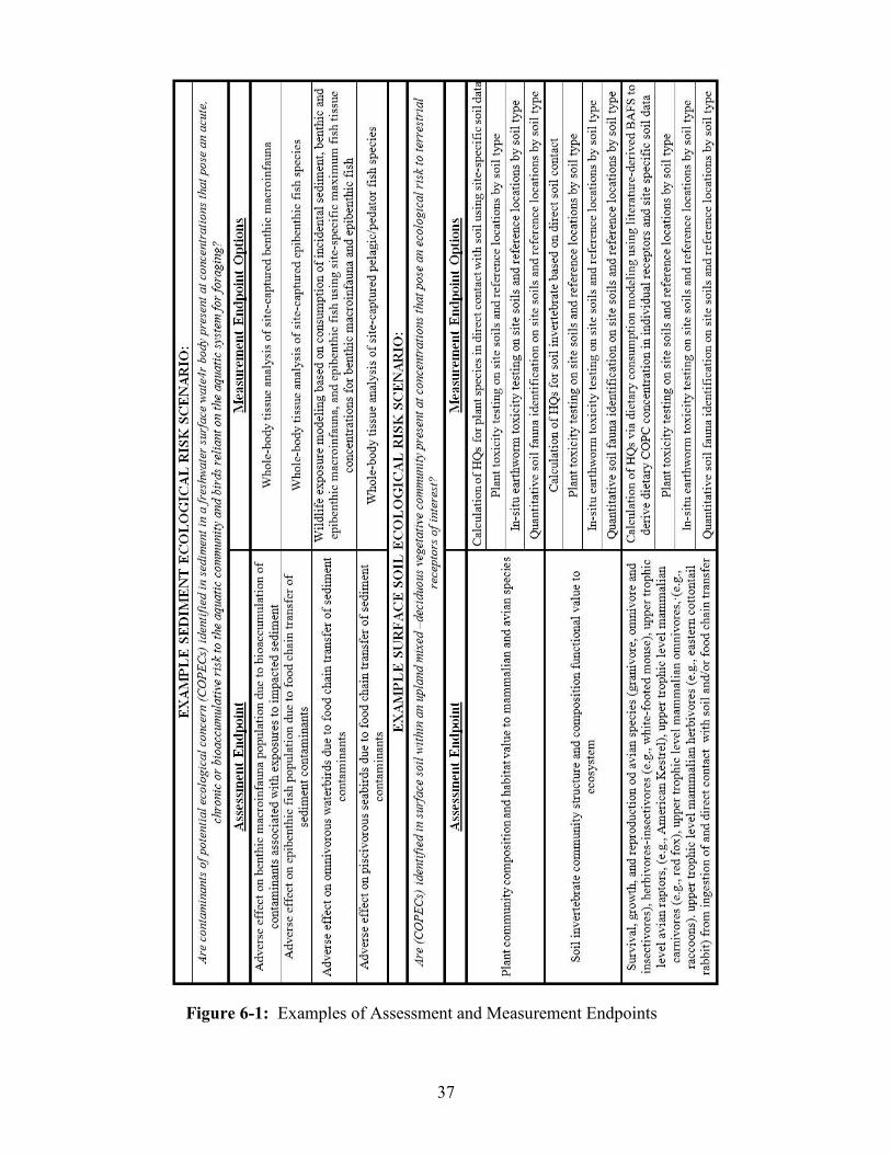
37
Figure 6-1: Examples of Assessment and Measurement Endpoints
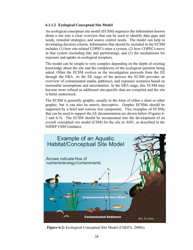
38
6.1.1.2 Ecological Conceptual Site Model An ecological conceptual site model (ECSM) organizes the information known about a site into a clear overview that can be used to identify data gaps and needs, remedial strategies, and source control needs. The model can help in developing decision criteria. Information that should be included in the ECSM includes (1) how site-related COPECs enter a system, (2) how COPECs move in that system (including fate and partitioning), and (3) the mechanisms for exposure and uptake in ecological receptors.
The model can be simple to very complex depending on the depth of existing knowledge about the site and the complexity of the ecological question being asked. Often the ECSM evolves as the investigation proceeds from the EE through the ERA. At the EE stage of the process the ECSM provides an overview of contaminated media, pathways, and exposure scenarios based on reasonable assumptions and uncertainties. In the ERA stage, this ECSM may become more refined as additional site-specific data are compiled and the site is better understood.
The ECSM is generally graphic, usually in the form of either a chart or other graphic, but it can also be merely descriptive. Graphic ECSMs should be supported by a brief and concise text component. Two examples of ECSMs that can be used to support the EE documentation are shown below (Figures 6-2 and 6-3). The ECSM should be incorporated into the development of an overall conceptual site model (CSM) for the site or AOC, as described in the NJDEP CSM Guidance.
Figure 6-2: Ecological Conceptual Site Model (USEPA, 2008c)
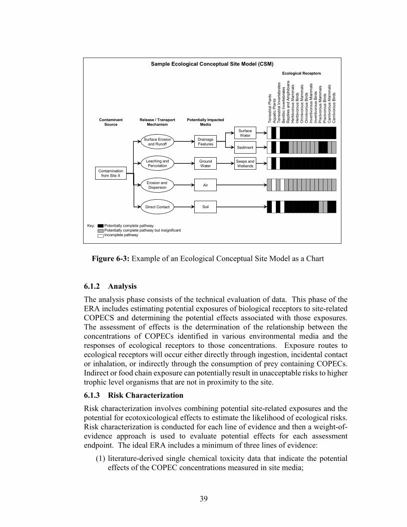
39
Terr
estri
al P
lant
sA
quat
ic P
lant
sTe
rres
trial
Inve
rtebr
ates
Ben
thic
Inve
rtebr
ates
Rep
tiles
and
Am
phib
ians
Her
bivo
rous
Mam
mal
sH
erbi
voro
us B
irds
Om
nivo
rous
Mam
mal
sO
mni
voro
us B
irds
Inve
rtivo
rous
Mam
mal
sIn
verti
voro
usBi
rds
Pis
civo
rous
Mam
mal
sP
isci
voro
us B
irds
Car
nivo
rous
Mam
mal
sC
arni
voro
us B
irds
Sample Ecological Conceptual Site Model (CSM)
Leaching andPercolation
Erosion and Dispersion
Direct Contact
Ground Water
Air
Soil
Surface Water
Sediment
Seeps and Wetlands
Contamination from Site X
Surface Erosionand Runoff
DrainageFeatures
Contaminant Source
Release / Transport Mechanism
Potentially ImpactedMedia
Ecological Receptors
Key: Potentially complete pathwayPotentially complete pathway but insignificantIncomplete pathway
6.1.2 Analysis The analysis phase consists of the technical evaluation of data. This phase of the ERA includes estimating potential exposures of biological receptors to site-related COPECS and determining the potential effects associated with those exposures. The assessment of effects is the determination of the relationship between the concentrations of COPECs identified in various environmental media and the responses of ecological receptors to those concentrations. Exposure routes to ecological receptors will occur either directly through ingestion, incidental contact or inhalation, or indirectly through the consumption of prey containing COPECs. Indirect or food chain exposure can potentially result in unacceptable risks to higher trophic level organisms that are not in proximity to the site.
6.1.3 Risk Characterization Risk characterization involves combining potential site-related exposures and the potential for ecotoxicological effects to estimate the likelihood of ecological risks. Risk characterization is conducted for each line of evidence and then a weight-of-evidence approach is used to evaluate potential effects for each assessment endpoint. The ideal ERA includes a minimum of three lines of evidence:
(1) literature-derived single chemical toxicity data that indicate the potential effects of the COPEC concentrations measured in site media;
Figure 6-3: Example of an Ecological Conceptual Site Model as a Chart
40
(2) biological surveys of the potentially affected system that indicate the actual state of the potentially affected environment; and
(3) toxicity tests with ambient media, which indicate the potential effects of COPEC concentrations measured in site media, if warranted or conducted.
Procedurally, the risk characterization is performed for each assessment endpoint by:
(1) comparing all measured COPECs against toxicological benchmarks (where possible, exposure-response gradients will be developed to help ascertain a more precise understanding of the potential for impacts on receptors);
(2) estimating the potential effects of the COPECs identified at the site; (3) estimating the effects of ambient media, based on the media toxicity test
results; (4) logically integrating the lines of evidence to characterize risks to the
endpoint; and (5) listing and discussing the uncertainties in the assessment.
6.1.3.1 Food Chain Modeling Food chain modeling, also known as dietary consumption modeling, dose modeling or wildlife exposure modeling, of contaminant uptake by wildlife species represents an important component of an ERA. Food chain modeling can be used to predict concentrations of contaminants in various environmental abiotic and biotic media. Potential dose is the primary metric used to quantify exposures to ecological receptors of interest (ROI) to chemical constituents. The amount of chemical present in food or water ingested, air inhaled, or material applied to the skin is known as the potential dose. A critical aspect of food chain modeling is the identification and use of exposure factors. These factors represent species-specific parameters related to food and water ingestion, body weight, home range, foraging range, and diet composition.
Exposure pathways that generally are of concern for ROI when conducting food chain modeling for an ERA include the following:
• Ingestion of contaminated food (plants or prey), particularly for contaminants with potential to bioaccumulate or biomagnify;
• Ingestion of contaminated water; and • Ingestion of contaminated soil or sediment. Although not frequently assessed, inhalation of contaminated airborne particles and vapors, and dermal absorption can also be considered, but are generally considered to be negligible. The majority of exposure is typically calculated using the oral exposure pathway. A series of equations are used to quantify the uptake by this pathway. The total exposure experienced by a particular ROI is the sum of the exposures to these pathways for each source and is generally described as the following:
E total = E food + E water + E incidental soil/sediment ingestion Where:

41
E total = total exposure from all pathways E food = exposure from food consumption
E water = exposure from water consumption
E incidental soil/sediment ingestion = exposure from soil or sediment consumption
Literature reference values for the independent parameters in each exposure model equation should always be supported by literature citations or site-specific information. Useful sources of exposure factors and information for developing soil, sediment, food, and water ingestion pathways are the Wildlife Exposure Factors Handbook (USEPA, 1993a) and Estimating Exposures of Terrestrial Wildlife to Contaminants (Sample, et al, 1994).
For exposure estimates to be useful in the assessment of risk to wildlife, the estimates should be expressed in terms of a body weight-normalized daily dose (e.g., milligrams of contaminant per kilogram of body weight per day (mg/kg/day)). Exposure estimates expressed in these units are then compared to toxicological benchmarks for wildlife or to doses reported in the scientific literature. Estimation of the daily contaminant dose to a particular species for each exposure pathway can be calculated by the general intake equation defined as:
ADD = CM*IR*FI*AF*BW-1
Where:
ADD = Average Daily Dose (mg COPEC/kg BW-day)
CM = Concentration of COPECs in media of concern (e.g., exposure point concentrations in sediment or soil [mg/kg dry weight], surface water [µg/l], or biota [mg/kg, wet weight])
Media concentrations are typically determined by a combination of measurements and modeling. A source is generally characterized by analysis, whereas movement into other media might be measured or modeled. In either case, spatial and temporal variations are important parameters that warrant consideration.
IR = Ingestion Rates (kg/day or L/day) IRs may be determined or estimated for each medium and pathway of concern for each representative species. IRs are expressed in terms of quantity of the medium (weight or volume) per day. When IRs for the representative species are not available, they may be estimated using data from surrogate species. In selecting surrogate data, taxonomic, anatomic, physiologic, and behavioral relationships and the quality of the studies are generally considered. A discussion of the scientific basis and rationale for the data set selection should be included in the ERA report.
For bird and mammal dose calculations, food (i.e., prey tissue) contaminant concentrations and the food ingestion rates should be expressed on a consistent basis (wet-weight or dry-weight). Food concentrations should be converted, as necessary, to correspond to the basis of the food ingestion rate
42
(i.e., wet weight or dry weight) using the food percent moisture data in the IR study, if available, or published literature food percent moisture data (USEPA 1993a, Figure 4-2).
Because soil and sediment data should be reported on a dry weight basis, ingestion rates for the incidental ingestion of soil or sediment should also be presented on a dry weight basis (USEPA 1993a, Figure 4-8).
For fish dietary dose calculations, the weight basis food of contaminant concentrations and the food ingestion rates may not be typically reported in dietary toxicity studies. Professional judgment should be used. For example, approximately 80% moisture could be assumed for the fish prey diet, based on USEPA 1993a, Section 4.1.2.
Equations used for converting ingestion rates and media contaminant concentrations between wet and dry weights should be provided in the ERA report.
FI = Fractional Intake (Exposure Frequency (day/year) * exposure duration (years)
The fraction of time spent in contact with contaminated media is generally defined as the time and area use factors. This may generally be approximated as the ratio of the area of the site-specific appropriate habitat to the foraging or home range area as appropriate (area use factor) and the amount of time per year a species spent in the habitat associated with the site (e.g., migratory considerations) (seasonal use factor). Consistent with ERAGS, when food chain modeling is conducted as part of the EE, and dietary concentrations are modeled from media concentrations, an FI equal to one is appropriate. When conducting a site-specific ERA that includes measured dietary concentrations (e.g., plant or animal tissue), using an FI that is less than one may be appropriate. Depending on site-specific circumstances, it may be appropriate to calculate a dose using both an FI of one and a less conservative FI to bound the range of potential ecological risk.
AF = Absorption Fraction (unitless) The AF is used if there are data to show that absorption by the exposure route in question is a fraction of the exposure route for which the literature reference dose was determined.
BW = Body weight of the ROI or representative surrogate (kg, fresh weight)
Although useful, modeling usually involves some range of uncertainty. Toxicity criteria may be pre-existing or derived and is expressed as reference dosages for terrestrial receptors or reference concentrations for aquatic receptors. Bioaccumulation in representative species that use both aquatic and terrestrial habitats, such as shorebirds or waterfowl, may be addressed as part of an aquatic or terrestrial assessment as appropriate.
43
Fugacity, which is described as the escaping tendency of a chemical species from a particular environmental compartment (e.g., air, water, sediment soil) is sometimes used to estimate tissue concentrations in biota to account for intermedia transfer; however, the results of these types of modeling efforts are often uncertain. It is recommended that predicted tissue residue levels only be used in a screening evaluation and that these values be verified with site-specific measurements to provide scientific validity to the process (e.g., bioaccumulation and field tissue residue studies).
The most common type of study reported in the literature is a contaminant bioaccumulation (uptake) study (Section 6.1.3.2). Where the potential for overestimating bioaccumulation by using conservative literature values to represent the site is substantial, additional evaluation of the literature for values more likely to apply to the site or a site-specific tissue residue study might be advisable. Bioaccumulation and field tissue residue studies typically are conducted at sites where contaminants are likely to accumulate in food chains and help to evaluate the degree to which a contaminant is transferred through a food chain.
A tissue residue study generally is conducted on organisms that are in the exposure pathway (e.g., food chain) associated with the assessment endpoint. Limited data are available to link tissue residue levels in the sampled organisms to adverse effects on those organisms. Literature toxicity studies usually associate effects with an administered dose (or data that can be converted to an administered dose), not a tissue residue level. Thus, the purpose of a field tissue residue study usually is to measure contaminant concentrations in foods consumed by the species associated with the assessment endpoint. This measurement minimizes the uncertainty associated with estimating a dose (or intake) to that species, particularly in situations in which several media and trophic levels are in the exposure pathway.
The concentration of a contaminant in the primary food (plant and prey) should also be linked to an exposure concentration from a contaminated medium (e.g., soil, sediment, water), because it is the medium, not the food chain, that will be remediated. Thus, contaminant concentrations should be measured in environmental media at the same locations at which the organisms are collected along contaminant gradients and at reference area locations. Temporally and spatially collocated samples of the contaminated media and tissue are needed to establish a correlation between the tissue residue levels and contaminant levels under evaluation.
Even if a complex dietary composition for each ecological receptor are available and evaluated, only those elements of the diet that have been analyzed for site-related contaminants, should be included as part of the diet in dose equations. The dietary composition, including exact percentages and elements of the diet, should be determined prior to initiating the risk assessment.
It is important that representative measurement endpoints (i.e., ecological receptors of interest (ROI)) are selected when using food chain modeling as a
44
measurement tool as part of an ERA. In order to do so, a thorough comprehension of the ecological structure (i.e., food-web) within each habitat-type of concern present at or immediately adjacent to your site/study area is necessary.
All classes of organisms (e.g., mammals, birds, fish, etc.) anticipated in the habitat(s) of concern should first be identified and documented. The identified classes of organisms within each habitat-type of concern should then be further refined based on their feeding strategies and trophic levels within the food webs. Completion of these two steps should help ensure that thorough consideration has been given to the dietary relationships amongst ROI when planning and preparing to conduct an exposure assessment using modeling as part of the ERA.
Once the habitat structure is understood, individual species for each class-specific feeding guild (e.g., mammalian herbivore, avian piscivore, etc.) can then be selected as measurement receptors. The final selection of measurement receptors should be carefully based on a consideration of the following five factors: 1) ecological relevance (i.e., functional attributes that effect the structural nature of a population), 2) exposure potential (i.e., metabolic rates and reproductive strategies) 3) known sensitivity (i.e., highly susceptible due to low tolerance), 4) socio-economic importance (e.g., game fish) and 5) availability of natural history information.
It is important that the selected ROI be representative of other species in the class-specific feeding guild such that the ROI ensures that risk to other species in the guild is not underestimated (i.e., highest exposure potential). Additionally, when identifying the dietary components of the measurement receptors of a guild, a general rule of thumb is to limit the number of prey items to the major prey items of the ROI.
Dietary exposure(s) to the measurement receptor(s) are then modeled, ultimately calculating an exposure dose. The exposure dose is represented by the dose of the COPEC received due to ingestion of abiotic and biotic media. Bulk chemistry data and/or preferably measured prey items (i.e., site-specific whole-body tissue contaminant concentrations) associated with the diet of the ROI are then used to calculate dietary estimates (i.e., daily dose) based on various exposure scenarios (i.e., maximum, mean and 95% upper confidence level), as appropriate. 6.1.3.2 Bioaccumulation In calculating levels of exposure, either direct toxicity to plants and wildlife or secondary toxicity to animals feeding on contaminated plants and animals, one issue that the investigator should be aware of is bioaccumulation. Bioaccumulation is the net extent to which a substance may be accumulated by an organism because of uptake from various media, including food. A list of contaminants considered to be bioaccumulative can be found in Table 4-2 of USEPA (2000c) Bioaccumulation Testing and Interpretation for the Purpose of Sediment Quality Assessment, Status and Needs. A similar concept is
45
bioavailability, which is the net extent to which the form of a chemical occurring in a medium is susceptible to being taken up by an organism. Bioavailability is (1) the cumulative expression of physical, chemical, and biological processes evident in air, water, soil, and sediment, and (2) biological factors present in the bodies, organs, tissues, or cells of exposed organisms that act to change that organism's rate of COPEC exposure (Suter et al., 2000).
To be consistent with the first two steps of ERAGS, the EE must assume that 100 percent of a particular COPEC that is identified in a particular media is available to the representative receptors being evaluated (N.J.S.A. 58:10B-12). While this is generally considered to be an overestimation of ecological risk, it provides a level of certainty if the conclusion of the EE is that no ecological risks are evident. However, in the ERA, the investigator should consider bioaccumulation when calculating the levels of exposure to be evaluated in the risk assessments, particularly in calculations of impacts to higher trophic level organisms through food chain transfer of a COPEC.
When sediment and soil chemistry data are available, but tissue chemistry is not, Sediment/Soil-to-Biota Bioaccumulation Factors (BSAFs) and Bioaccumulation Factors (BAFs), respectively, can be estimated for select compounds using published accumulation factors (http://www.erdc.usace.army.mil/Media/Fact-Sheets/Fact-Sheet-Article-View/Article/832015/biota-sediment-accumulation-factor-bsaf-database/, and http://www.epa.gov/med/Prods_Pubs/bsaf.htm). Such data should be used with caution because it is not site specific and could overestimate or underestimate accumulation.
The BSAFs and BAFs are the ratios of tissue concentrations, wet weight, to the sediment- and soil-associated concentrations, dry weight, of organic compounds or metals (Kubiak, et.al., 2007; USEPA and USACE, 2008; USEPA and USACE, 2014). A site-specific BSAF or BAF can be empirically determined through collection and chemical analysis of collocated sediment or soil, respectively, and organism tissue. Because some contaminants bind to organic matter in sediment and soil or to lipids in the tissue of exposed organisms, site-wide BSAF and BAF values need to be normalized for TOC and for lipid content (USEPA, 2009c).
In ERAs for complex situations, studies to more accurately predict bioaccumulation and the movement of a COPEC through the environment should be considered. Generally, these studies will consist of field-collected tissue samples (both plant and animal) at different trophic levels of the environment. As noted in ERAGS, the purpose of a field-collected tissue residue study usually is to measure contaminant concentrations in foods consumed by the species associated with the assessment endpoint.
The primary purpose of tissue residue analysis for ERA is to determine whole body contaminant concentrations in prey consumed by the receptor of interest. This analysis provides an estimate of the contaminant dose to the receptor of
46
interest, which can be compared to literature-based tissue residue effects levels (toxicity reference values (TRV)) for the purpose of estimating risk.
Tissue residue data can play an important role at different stages in the process of evaluating hazardous waste sites, including ecological risk assessment, modeling conducted to evaluate different remedial alternatives, and monitoring necessary to determine the effectiveness of remediation (Field, 1998; Canadian Council of Ministers of the Environment, 1999; Jarvinen and Ankley, 1999). Evaluation of tissue residue effects relies on the identification of whole body concentrations of a chemical that has been demonstrated to be associated with adverse effects on a target organ or system in a variety of aquatic organisms or phylogenetic groups. Tissue residue effects are contaminant and taxon specific threshold concentrations measured in biological tissue above which adverse effects of ecological relevance would be anticipated to occur based on field or laboratory studies. Data may be used from a surrogate species when studies for a particular species cannot be found. Tissue residue effects are generally based on mortality, reproductive or growth endpoints, which are most relevant for estimating the potential for adverse population level effects. Databases for tissue residue effect levels include the ERED database (Environmental Residue Effects Database, https://ered.el.erdc.dren.mil/).
Prerequisites for Bioaccumulation Studies In the event field tissue collection is not feasible, the investigator may choose to conduct field or laboratory bioaccumulation studies using laboratory cultured organisms. Bioaccumulation studies can be expensive and time-consuming. Before conducting a bioaccumulation study, the toxicity of the soil or sediment should be assessed either through historical toxicity data or through screening toxicity studies (exposing toxicity test organisms for one to ten days to determine toxic effect). Field reference locations should also be screened to ensure that they are appropriate for inclusion in testing. The effort and expense of a bioaccumulation study are unnecessary if site soil or sediment is determined to negatively impact organism survival, based on toxicity tests or field evaluations. If survival is significantly reduced, bioaccumulation is not the primary concern.
Bioaccumulation Study Design Considerations Bioaccumulation studies require careful consideration of many variables including physical and chemical conditions of the matrices being tested, sample selection, sample volume (i.e., tissue mass requirements), laboratory QA/QC (e.g., replicates, tissue preparation and processing). When considering the selection of commercially viable shellfish species as test organisms, the investigator is advised to contact the Bureau of Marine Water Monitoring (http://www.state.nj.us/dep/wms/bmw/about.htm). Permits may be required.
Physicochemical Data Needs Bioaccumulation studies can be laboratory-based (e.g., ASTM, 2010; USEPA, 2000a), or performed in situ (e.g., Burton et al., 2004; ASTM, 2007a).
47
Bioaccumulation in sediment and soil is controlled by many physicochemical factors including TOC, pH, redox potential, salinity, temperature, grain size, sulfides, the types of contaminants and their concentrations, and the lipid content of receptor organisms. Additional variables, including contaminant soil sorption coefficients, water solubility, hydrolysis, photolysis, nutrient concentrations (Ca, Fe, Mg, P, K, Na, sulfate, ash content, cation exchange capacity, and Kjeldahl nitrogen), further control bioaccumulation in soil. Test organism selection should take these physiochemical factors into account when selecting a study organism to avoid stressing the study organisms.
Salinity is an important example of a study design consideration. Salinity can cause osmotic stress on test organisms and can impact the bioavailability of sediment contaminants. If marine sediment is laboratory-tested at low salinity, some contaminants may become more bioavailable than they would be under higher salinity conditions. This would potentially yield artificially high BAFs and produce results that are not representative of site conditions.
Some coastal, estuarine, and tidal sites can pose significant salinity challenges, with upstream samples in freshwater or low salinity conditions and downstream samples in higher salinity or marine conditions. It is desirable to perform a single bioaccumulation study using the same test organism for all samples. However, it is usually not feasible to acclimate a single batch of test organisms to a wide range of salinities, and changing the salinity of the samples to suit the test organism could potentially alter the bioavailability of COPECs and yield results that are not representative of site conditions. Several species could be used, but different species may accumulate COPECs in widely varying rates and the results may not be comparable. Issues with acclimating a single species or using more than one species should be considered during study design.
In the aquatic environment, adjustments may be considered to account for bioavailability in surface water calculations such as water hardness and pH, particularly with soluble metals.
Other examples of nonchemical stressors in soil bioaccumulation studies are soil nutrients and moisture. When testing plants, it is important to know the nutrient content of the soil to differentiate between effects caused by chemical toxicity and effects caused by lack of nutrients. Most soil-dwelling organisms thrive in a relatively narrow range of soil moisture percentage. Too much moisture will potentially drown invertebrates or plants, while too little moisture will desiccate them.
Sample Selection After completing the toxicity test phase of the bioaccumulation study, investigators should determine whether the tissue samples should be submitted for COPEC analysis. When choosing test tissue samples to submit for analysis, it is important to select only tissue from those soil or sediment samples that showed no significant reduction in organism survival, as compared to the laboratory control or reference sample. If survival is significantly reduced, bioaccumulation is not the primary concern. If a significant percentage of the
48
organisms exposed to a soil or sediment sample did not survive the test period, it is highly likely that the tissue COPEC burden accumulated by the surviving organisms would not be representative and could be misleading. It is also important to include only those test organisms that survived the entire test period for tissue analysis. All dead organisms should be recorded and discarded. Inclusion of dead organisms in tissue analysis would not be representative and could bias the study. Tissue Mass Requirements Depending on the list of COPECs, the analytical tissue mass requirement may be quite high (50 to 70 grams per sample for a full suite of organic and inorganic analytes).
Marine/estuarine bioaccumulation studies with oligochaete worms (e.g., Nereis virens or Neanthes arenacoedentata) or bivalves (e.g., clams, mussels or oysters) can easily be designed to yield sufficient tissue mass because the test organisms are relatively large. This allows analysis of tissue samples from individual test replicates, allowing robust statistical comparison of each sediment sample. However, freshwater bioaccumulation studies are typically performed with much smaller polychaete worms (e.g., Lumbriculus variegatus) or bivalves (e.g., fingernail clams, Corbicula fluminea). Individual L. variegatus weigh approximately 0.015 grams, requiring thousands of worms to make up a 50-gram tissue mass requirement. Because it is not feasible to set up multiple replicate samples with thousands of worms, it is best to limit use of L. variegatus to sediment samples with COPEC lists with a small analytical tissue mass requirement.
Some bioaccumulation studies with soil organisms (e.g., earthworms or plants) can easily be designed to yield sufficient tissue mass because the test organisms can be relatively large. Testing can be initiated with worm species that are large enough to yield sufficient tissue at test termination. Plant bioaccumulation studies can be performed using species that will grow sufficiently by test termination to yield the desired tissue mass. This allows analysis of tissue samples from individual test replicates, allowing robust statistical comparison of each soil sample. The portion of plant to be assayed needs to be determined on a case by case basis. For example, if data are to be used for dietary exposure modeling, Arrow arum fruit is a preferred food of wood ducks, and all portions of aquatic plants (e.g., roots, basal portions, stems, leaves) and basal portions of Phragmites can be consumed by muskrats. Also, roots and leaves of aquatic plants can be consumed by benthic omnivorous fish, such as common carp, catfish, white perch, etc.
However, some bioaccumulation studies can be performed with much smaller organisms (e.g., springtails or potworms), depending on study objectives. Individual springtails or potworms are very small, requiring hundreds of organisms to make up a 50-gram tissue mass requirement. Because it is usually not feasible to set up multiple replicate samples with hundreds of organisms, it
49
is best to limit use of smaller invertebrates to soil samples with COPEC lists with a small analytical tissue requirement.
Laboratory QA/QC Objectives Replicates
As is required with any toxicity study, appropriate replication is necessary to ensure comparability between soil or sediment samples and laboratory control or reference samples. Bioaccumulation studies should be designed to produce the required analytical tissue mass from each test replicate. If sufficient tissue mass is not possible from each replicate, compositing between replicates is acceptable. However, compositing reduces the statistical power of the study. If all test replicates have to be composited to a single sample, statistical comparisons are not appropriate and the study may not meet the data quality objectives for inclusion in a risk assessment. Where sufficient historical data are available, a power analysis (Zar, 1984) is often useful to determine how many test replicates may be necessary to ascertain differences between soil or sediment sampling locations or reference area soils.
Tissue Preparation and Processing
Because even a small amount of potentially contaminated soil or sediment can significantly bias any tissue analysis, it is critical to remove all traces of soil or sediment from the test organisms before submitting the tissue for COPEC analysis. For example, plant roots should be thoroughly rinsed and carefully examined to ensure that all soil is removed. Earthworms and other organisms that ingest and process soil should be depurated for a time sufficient to ensure that the digestive tract is empty. While 24 hours is an acceptable depuration period (ASTM, 2004), studies have indicated that different species may require 48 hours for sufficient depuration, and some other species may require dissection and rinsing of the digestive tract (Arnold and Hodson, 2007).
All tissue samples should be analyzed for COPECs, percent moisture and percent lipids (as appropriate). In addition to the analysis of tissue samples, bioaccumulation studies should include analysis of all site soil and/or sediment samples, reference samples and laboratory control samples for COPECs, grain size, TOC and pH. Soils used for plant toxicity or bioaccumulation studies should also be analyzed for soil nutrient concentrations.
While there are many laboratories that can produce acceptable analytical results for soil and sediment samples, not all laboratories are capable of tissue analysis. Tissue processing requires specialized equipment in addition to the standard analytical instrumentation, and some laboratories cannot work with small samples. Tissue samples, particularly samples with high lipid content, may also present analytical interference that can yield excessively high analytical detection limits for insufficiently experienced laboratories.
It is critical to discuss bioaccumulation study objectives with both the toxicity testing laboratory and the analytical laboratory, to ensure that data quality objectives are met.
50
6.1.3.3 Toxicity Reference Values Toxicity reference values (TRV) are literature-based levels defined as a dose above which ecologically relevant effects might occur in wildlife species following chronic dietary exposure and below which it is reasonably expected that such effects will not occur (USEPA, 2005a). TRVs provide a basis for estimating whether the exposure to COPECs at a site is likely to result in adverse ecological effects (e.g., survival, growth, and reproduction of wildlife species). TRVs can also be used in the development of ecological risk-based remediation goals (Section 7.0). TRVs are generally based on NOAELs and LOAELs from laboratory and/or field-based studies reported in the scientific literature (USEPA, 2005a and Sample et al., 1996). Selected TRVs are presented along with justification for final selection in the ERA report.
Risks are estimated for appropriate feeding guilds by comparing the results of the measured or modeled dietary contaminant doses to receptors of concern to the TRVs. The ratio of these two numbers is called a Hazard Quotient (HQ). HQs equal to or greater than one (HQ ≥ 1) are typically considered to indicate potential risk to ecological receptors. If an HQ suggests that effects are not expected to occur for the average individual, then the effects are likely to be insignificant at the population level; however, if an HQ indicates risks are present for the average individual, then risks may be present for the local population. NOAEL-based and LOAEL-based HQs should be developed to bound the risk estimates.
The basic equation used for calculation of an HQ value for exposure of a wildlife receptor to a chemical by ingestion of an environmental medium is:
HQi, j, r = ADD oTRVi,r
where:
HQi,j,r = HQ for exposure of receptor “r” to COPEC “i” in medium “j” ADD = Average Daily Dose (mg/kgBW-day) oTRVi,r = Oral TRV for COPEC “i” in receptor “r” (mg/kg-day)
Because all receptors are exposed to more than one environmental medium, the total hazard to a receptor from a specific COPEC is calculated as the sum of HQs for that COPEC across all media:
HQi, r = Σ HQi, j, r
Selection of Toxicity Reference Values
The approach provided below is consistent with USEPA as mandated by the Brownfield and Contaminated Site Remediation Act by “use of the guidance and regulations for exposure assessment developed by the United States Environmental Protection Agency pursuant to the ‘Comprehensive Environmental Response, Compensation, and Liability Act of 1980,’ 42 U.S.C. § 9601 et seq. and other statutory authorities as applicable” and provides the
51
user with a framework from which to develop TRVs; however, as with all guidance documents issued by the NJDEP, the person conducting the remediation may deviate from this approach and propose an alternate TRV based on site-specific circumstances provided that adequate justification is provided.
The first tier of TRVs to consider are those used in the Focused Feasibility Report for the Lower Eight Miles of the Lower Passaic River (USEPA 2014), Appendix D. These TRVs were vetted by NJDEP, USEPA, USFWS, and NOAA; have been used in support of the Record of Decision (ROD) for the Passaic River Lower Eight Mile Superfund site; are considered sufficiently conservative; and will not be subject to further scrutiny during SRWMP’s inspection and review process if selected and used in the ERA. Table 1 provides the list of TRVs from the Focused Feasibility Study Report for the Lower Eight Miles of the Lower Passaic River, (2014) – Table 4-14 , available at (http://passaic.sharepointspace.com/Public%20Documents/2014-02-20%20Appendix%20D%20Risk%20Assessment.pdf).
The second tier of TRVs are USEPA’s Ecological Soil Screening Levels (Eco-SSLs, USEPA, 2005a et seqq.) and are recommended for contaminants not included on Table 1, or as an alternative. When using TRVs from the contaminant-specific Eco-SSL documents, the NOAEL- and LOAEL-based TRVs should be those used by USEPA for the derivation of Eco-SSLs. The Eco-SSLs are most typically the highest bounded NOAEL that is lower than the lowest bounded LOAEL for reproduction, growth and/or mortality (“bounded” means a study from which a NOAEL-LOAEL pair was determined). However, Eco-SSLs may have been derived for select contaminants from the geometric mean of NOAELs for growth and reproductive effects from peer-reviewed documents; in that case, an appropriately conservative LOAEL should be selected. If TRVs other than these were used by USEPA to develop the Eco-SSLs, then those TRVs should be used.
The third tier of TRVs is taken from literature sources. Caution should be used if these literature sources were rejected by USEPA during derivation of the Eco-SSLs. Appropriate justification should be provided for use of a particular literature source and for the TRVs chosen from that literature source. Justification can include the type of study, receptor used and dosing methodologies, as well as other factors. Notwithstanding the use of statistical evaluations in USEPA 2005a, it is recommended that third-tier TRVs be developed from a single study or receptor with bounded NOAELs and LOAELs and should not be based on statistical evaluations of multiple TRVs/studies across several receptors, as errors and uncertainty can be introduced into the calculations; moreover, it expected that this third tier will be used for less common contaminants, with potentially too few studies available for statistical evaluations.
If TRVs are used to determine ecological risk-based remediation goals, they will be reviewed by NJDEP SRWMP in that context, because ecological remediation goals require Department pre-approval (N.J.A.C. 7:26E-4.8(c)3).
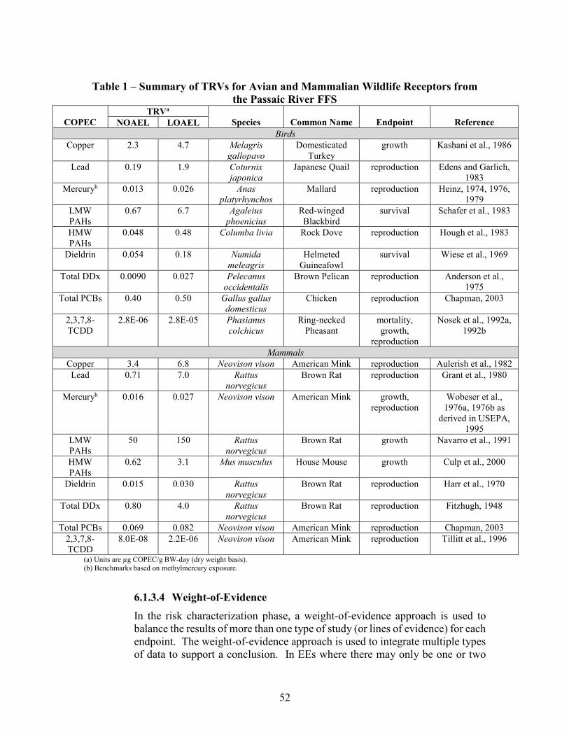
52
Table 1 – Summary of TRVs for Avian and Mammalian Wildlife Receptors from
the Passaic River FFS
COPEC TRVa
Species
Common Name
Endpoint
Reference NOAEL LOAEL Birds
Copper 2.3 4.7 Melagris gallopavo
Domesticated Turkey
growth Kashani et al., 1986
Lead 0.19 1.9 Coturnix japonica
Japanese Quail reproduction Edens and Garlich, 1983
Mercuryb 0.013 0.026 Anas platyrhynchos
Mallard reproduction Heinz, 1974, 1976, 1979
LMW PAHs
0.67 6.7 Agaleius phoenicius
Red-winged Blackbird
survival Schafer et al., 1983
HMW PAHs
0.048 0.48 Columba livia Rock Dove reproduction Hough et al., 1983
Dieldrin 0.054 0.18 Numida meleagris
Helmeted Guineafowl
survival Wiese et al., 1969
Total DDx 0.0090 0.027 Pelecanus occidentalis
Brown Pelican reproduction Anderson et al., 1975
Total PCBs 0.40 0.50 Gallus gallus domesticus
Chicken reproduction Chapman, 2003
2,3,7,8-TCDD
2.8E-06 2.8E-05 Phasianus colchicus
Ring-necked Pheasant
mortality, growth,
reproduction
Nosek et al., 1992a, 1992b
Mammals Copper 3.4 6.8 Neovison vison American Mink reproduction Aulerish et al., 1982 Lead 0.71 7.0 Rattus
norvegicus Brown Rat reproduction Grant et al., 1980
Mercuryb 0.016 0.027 Neovison vison American Mink growth, reproduction
Wobeser et al., 1976a, 1976b as
derived in USEPA, 1995
LMW PAHs
50 150 Rattus norvegicus
Brown Rat growth Navarro et al., 1991
HMW PAHs
0.62 3.1 Mus musculus House Mouse growth Culp et al., 2000
Dieldrin 0.015 0.030 Rattus norvegicus
Brown Rat reproduction Harr et al., 1970
Total DDx 0.80 4.0 Rattus norvegicus
Brown Rat reproduction Fitzhugh, 1948
Total PCBs 0.069 0.082 Neovison vison American Mink reproduction Chapman, 2003 2,3,7,8-TCDD
8.0E-08 2.2E-06 Neovison vison American Mink reproduction Tillitt et al., 1996
(a) Units are µg COPEC/g BW-day (dry weight basis). (b) Benchmarks based on methylmercury exposure.
6.1.3.4 Weight-of-Evidence In the risk characterization phase, a weight-of-evidence approach is used to balance the results of more than one type of study (or lines of evidence) for each endpoint. The weight-of-evidence approach is used to integrate multiple types of data to support a conclusion. In EEs where there may only be one or two
53
lines of evidence (e.g., COPECs and ESNRs), a weight-of-evidence approach may either be unnecessary or simplistic. However, in more complex ERAs, multiple studies or lines of evidence may need to be evaluated for each endpoint to reach a conclusion regarding the level of risk.
The weight-of-evidence begins by summarizing the findings of each line of evidence for each assessment endpoint. If the endpoint is associated with the exceedance of some threshold, then the weight-of-evidence evaluation will first evaluate each line of evidence to determine whether (1) the findings of the study can be definitively identified as an exceedance of the threshold, (2) whether it can be definitively identified as not exceeding the threshold, or (3) the findings are ambiguous. Then, the findings of all lines of evidence for each assessment endpoint should be summarized to reach a decision as to whether it is likely or unlikely that the threshold was exceeded.
If all lines of evidence support a conclusion, then the process of determining risk has been completed with a high degree of confidence. However, if there is bias or uncertainty in the various lines of evidence, then a true weighing of evidence should occur. As noted in Suter et al. (2000), the lines of evidence within each assessment endpoint should be evaluated as per the following parameters:
• Relevance –greater weight is given if the measure of effect is more directly related to the assessment endpoint;
• Exposure and Response –greater weight is given to those studies that show a correlation between the magnitude of the response to the magnitude of the exposure;
• Temporal Scope –greater weight is given to those results that relate to the time constraints and variations of the assessment endpoint;
• Spatial Scope – greater weight is given to those results that accurately reflect the location of the site being assessed;
• Data Quality – greater weight is given to data that meet appropriate DQOs; • Data Quantity – greater weight is given to those studies that have an
adequate amount of data to meet statistical confidence; and • Uncertainties – greater weight is given to those studies that have the least
uncertainties.
6.2 ERA Data Development This section describes the various tools and methods that may be employed to more accurately characterize ecological risk. Many of the tools identified (e.g., sediment toxicity test, tissue sampling) are designed to take into account site-specific bioavailability, and by doing so, offer a more refined measure of toxicity than simply comparing bulk sediment chemistry results to generic screening values.
The subsections that follow are organized by media (surface water, sediment, and soil) and include a description of some of the tools and methods commonly used to evaluate ecological risk. The selection of the tools and methods to employ at a particular site will be dependent upon site-specific factors such as habitat type, ecological receptors
54
present, type of COPECS, ability of the contaminant to bioaccumulate or biomagnify, and complexity of the site under investigation (multiple media contamination).
6.2.1 Surface Water Basic surface water sampling guidance is provided in Section 5.3.3.2. The following sections describe data development issues and the suggested protocols to be used in more comprehensive surface water sampling programs.
6.2.1.1 Sampling Plan Design for Study and Reference Areas The investigator is referred to N.J.A.C. 7:26E-2.1 for appropriate analytical protocol and quality assurance requirements. The investigator is also referred to Section 10.0 of this document for additional guidance on QA/QC and the preparation of quality assurance plans.
If a discharge is observed or the preliminary surface water results, collected during the EE phase (Sections 5.3.2.2 and 5.3.3.2), reveal the presence of contaminants at concentrations above their respective aquatic chronic SWQS or appropriate ESC, then additional investigations are required to support the ERA. Pursuant to N.J.A.C. 7:26E-4.8(c)1, it is imperative that the area of impact be accurately delineated to the appropriate SWQS or ESC. Professional judgment is required to develop an appropriate sampling strategy, which will be determined by the size and characteristics of the surface water body being investigated. Smaller water bodies may be investigated with the collection of additional grab samples. The sampling of larger water bodies can be accomplished with additional sampling along transects that typically run perpendicular to the banks of the water feature under investigation. The number of samples, number of transects, number of samples per transect, and depth of the sample in the water column are site-specific and depend on factors such as magnitude of discharge, size of water feature, water depth, etc.
Surface water in tidally influenced water bodies should be sampled at both low and high tides at several locations to better define the area of impact as it relates to the tidal cycle. Corresponding background area samples should also be collected with each tidal cycle and should be located upgradient of the mixing zone to ensure they are located outside the realm of potential site impacts.
The decision to collect additional background area locations should consider: (1) the relationship of the existing background area locations to the site location; (2) the complexities of the water body; and (3) the need for increased statistical significance in the relationship between the site and background area samples. The decision may also be based on a need to add samples at various depths, to obtain information on different habitats, or to account for temporal changes in discharges or in water level.
If the surface water contamination is attributed to an ongoing groundwater discharge, then an evaluation of sediment pore water concentrations to evaluate potential impacts to the benthic community should be conducted. Additional guidance on the evaluation of this ground water discharge pathway can be found in Section 6.2.2.3.
55
In some instances, contaminants detected in surface water may not have a corresponding aquatic chronic SWQS. The investigator may choose to develop a site-specific standard. In lieu of developing a site-specific standard, the investigator may provide an alternate ESC from literature sources, or may choose to complete a surface water toxicity test to determine potential adverse impacts to aquatic receptors. The SWQS provide guidance on how to develop an aquatic chronic surface water standard at N.J.A.C. 7:9B-1.14(f) based on two USEPA documents:
• Guidelines for Deriving Numerical National Water Quality Criteria for the Protection of Aquatic Organisms and Their Uses (USEPA, 1985b) http://water.epa.gov/scitech/swguidance/standards/criteria/aqlife/upload/85guidelines.pdf
• (USEPA, 1995b) Updates: Water Quality Criteria Documents for the Protection of Aquatic Life in Ambient Water (EPA-820-B-96-001) (1995 Updates) https://nepis.epa.gov/Exe/ZyNET.exe/20002924.TXT?ZyActionD=ZyDocument&Client=EPA&Index=1995+Thru+1999&Docs=&Query=&Time=&EndTime=&SearchMethod=1&TocRestrict=n&Toc=&TocEntry=&QField=&QFieldYear=&QFieldMonth=&QFieldDay=&IntQFieldOp=0&ExtQFieldOp=0&XmlQuery=&File=D%3A%5Czyfiles%5CIndex%20Data%5C95thru99%5CTxt%5C00000005%5C20002924.txt&User=ANONYMOUS&Password=anonymous&SortMethod=h%7C-&MaximumDocuments=1&FuzzyDegree=0&ImageQuality=r75g8/r75g8/x150y150g16/i425&Display=hpfr&DefSeekPage=x&SearchBack=ZyActionL&Back=ZyActionS&BackDesc=Results%20page&MaximumPages=1&ZyEntry=1&SeekPage=x&ZyPURL
Aquatic chronic surface water standards developed using the above methodologies must be approved by the NJDEP prior to use (N.J.A.C. 7:9B-1.14(f)). 6.2.1.2 Surface Water Habitat Assessments and Community Surveys Habitat surveys and community surveys can serve to support the ERA process. Although a habitat survey has some credible value without a community survey and can enhance the qualitative aspects of the risk assessment, a community survey should not be conducted without a habitat survey. These assessments and surveys are generally conducted at both the site of concern and a reference area.
Habitat Assessment Habitat is a key component of the ecosystem and an integral part of a site assessment. Without an understanding of the habitat characteristics of a surface water body, any survey of fish, invertebrates, plants, etc., will be out of context because no assumption of a “healthy population” can be ascertained. Additionally, the habitat assessment incorporates the potential limitations on a community that may not be attributable to the COPECS under investigation.
56
For the purposes of surface water, habitat is considered to be both aquatic and riparian because this is the habitat that most directly influences the aquatic community.
Although numerous habitat assessment protocols are available and may be acceptable, the visual-based habitat assessment described in Rapid Bioassessment Protocols for Use in Streams and Wadeable Rivers (USEPA, 1999b) is recommended along with the habitat assessment protocol included in Field and Laboratory Methods for Macroinvertebrate and Habitat Assessment of Low Gradient, Nontidal Streams (USEPA, 1997b) for habitat that is more lentic. These protocols, when used correctly, provide a high-quality assessment in a short time with minimal cost.
When planning a habitat assessment, the area to be assessed should be the same as the area planned for a community survey (if one is planned) although for certain parameters a “wider” view of the site may be necessary. If the community survey is conducted on the same day, care should be taken not to disturb the sampling habitat. Spring and summer are ideal for a habitat assessment.
These habitat assessments provide field-ready worksheets (Appendix A) for grading, on a scale of 0-20, a select set of habitat characteristics that can be summed to a final score that can help characterize the degradation of a particular area. These assessments can then be included in the lines of evidence used during different stages of the risk assessment. Three sets of worksheets based on gradient are included. It is important to use the worksheets that best fit the site being assessed.
The habitat assessment should be conducted by a biologist or ecologist familiar with the protocols in the above documents and with the environmental qualities in the area to be assessed. It is recommended that at least two of these qualified personnel conduct the habitat assessment at the same time, but separately, so that any discrepancies in the qualitative evaluations can be discussed and agreed upon before finalizing scores. During the collection of habitat data, basic physicochemical data on the surface water (e.g., pH, DO, conductivity, salinity, temperature, and turbidity) should also be collected.
Community Surveys Community surveys measure current biological conditions. These surveys are the only way to directly measure the structure and function of a community. Combined with the habitat assessment, this information complements and can enhance the contaminant information collected at a site and can provide additional lines of evidence to support conclusions and management decisions at various stages of the risk assessment process.
There are two basic survey types: community structure surveys and community function surveys. Community structure is the measurement of biotic characteristics (e.g., species abundance, diversity, and composition) at a point in time. Community function is the measurement of rate processes (e.g., species
57
colonization rates) of the ecosystem. Although both surveys can provide value depending on the biological questions being asked in the risk assessment, most often, structural surveys are conducted because they are generally less resource-intensive in terms of time and cost.
In surface water environments, a variety of community surveys can be conducted, and these data can be used in various ways. Most commonly accepted and often the easiest to conduct and evaluate are statistically based indices that have been developed by numerous states for a range of ecosystem components. However, other surveys may be applicable based on seasonal variation, natural characteristics of the site, or other project demands.
What is important is that the parameters of the survey accurately reflect the data acquisition needs of the ERA, including the community selected, sampling methods, and spatial and temporal planning. Surveys that use more than one taxonomic group and more than one trophic and tolerance level in each group tend to be more robust. Additionally, sampling protocols that account for subhabitats and seasonal life-cycle changes will yield a more representative data set.
Generally accepted aquatic community surveys include fish, macroinvertebrates, algae, and zooplankton. Fish and macroinvertebrates are typically used in lotic environments, plants are generally used in wetland environments, and algae are often used in lentic environments. Sampling methods for these groups are discussed in Sections 6.2.1.3, 6.2.2.4, and 6.4.1.
6.2.1.3 Biological Sampling of Fish and Other Aquatic Organisms As part of the completion of an ERA, the investigator may choose to collect aquatic biota for either fish tissue analysis or community survey purposes. When fish are collected for chemical analysis of tissue, whole body analysis is required to evaluate the representative dose to predator species. Species based on feeding guilds and habitats present in the ESNR should be targeted for collection. For example, it may be appropriate to target water column feeders (e.g., white perch), bottom dwellers (e.g., brown bullhead, channel catfish, white catfish, eel), and large forage range fish (largemouth bass, smallmouth bass, striped bass, rock bass). The analysis of individual fish is paramount, with compositing recommended only when necessary to achieve the minimum tissue mass for chemical analysis. If compositing is used, it is recommended that only fish from one habitat or feeding area be combined. Cross-species compositing should not be performed.
Professional judgment may be needed to decide whether to composite for full scan analysis versus analysis of individual fish in accordance with a site-specific analytical hierarchy. For composite samples, it is recommended that the length of the smallest fish in a sample should be > 75% of the largest; the sex, weight, and length of each fish used for each sample should be recorded. Fish tissue data should be reported on a wet-weight basis because representative contaminant concentrations are needed for dietary modeling to higher trophic level receptors. Lipids and percent moisture should be analyzed in each sample.
58
Generally, when fish are selected for community survey purposes, the goal is to collect all species in a defined area. Two common fish collection methods for biological survey purposes are seining, which has a limited efficacy depending on habitat, and electrofishing, which, when used appropriately, greatly increases the number of available individuals captured. Often a seine is set on the downstream end of the selected survey reach to ensure capture of all stunned individuals including those not captured by the personnel at the electrofishing location itself. In most cases, a pulsed DC current is used because this keeps mortality low. An AC current may be needed in streams with low conductivity. Other methods, such as gill nets and minnow traps, can be used.
The type of electrofishing gear used (e.g., backpack, boat, barge) is dependent on the stream characteristics. The selection of the reach used should be reflective of the data needs for the risk assessment and should include all major subhabitats characteristic of the area. Sampling should be conducted in June through early October during normal flow conditions. Sampling during the winter, at night, and during atypical flow conditions will not produce a representative data set.
Electrofishing should only be performed by trained personnel. Proper permits must be obtained (http://www.nj.gov/dep/fgw/scicolperm.htm). Detailed procedures are given in the Rapid Assessment Protocols for use in Wadeable Streams and Rivers (USEPA, 1999b) including QA/QC and important safety precautions.
The method used most often to collect individual fish is to work slowly upstream capturing all stunned fish as they drift. These fish are then placed in live wells (situated outside of the current impact area) to reduce mortality. Once the fish in the selected reach have been collected, the specimens are identified in the field to species level, and all data are recorded on data sheets. Fish less than 20 mm long are not included in tallies because of their seasonality and limited response to the sampling method. Other data may be collected depending on the specific study design. Identification should be made by an experienced biologist or ecologist familiar with New Jersey fishes. Once all organisms have been identified, the fish are released back into the stream. Voucher specimens may be collected as the needs of the project dictate.
Physicochemical and habitat data should be conducted on the same day as the survey is conducted. If the data collection requires disturbing targeted habitat, it should be conducted either after the survey is complete or just outside the survey area.
During collection of fish, sampling personnel should record observations such as species identification, number of species, sex, age, length, weight, disease, and presence of gross histopathological anomalies that may be present in such areas as the gills, fins, and eyes. Other observations of the general physical health of the specimens may be made as necessary (removal of a scale or spine for aging, determination of sex, and observations of overall health such as parasites, fin erosion, skin lesions). If field dissections of captured fish are
59
conducted, observations of the internal organs, such as liver, muscles, and urogenital organs, should be made to assess the presence of any gross abnormalities. Additionally, field observations of behavioral changes (e.g., twitching, gasping, long-axis whirling, and convulsions) should be made.
If site COPECs are known to be associated with histopathological effects on fish, a subset of the fish collected should be subjected to internal histopathological analysis (e.g., this analysis serves as a measurement endpoint associated with the assessment endpoints of survival, growth, development, reproduction, and maintenance of healthy fish populations). Laboratory methods for histopathological evaluation can be found in EPA (1995c) and Schmitt and Dethloff (2000).
Biological sampling for primary producers, such as benthic algae and plankton, may be needed for specialized evaluations such as a food web study. Refer to Appendix B for detailed procedures.
6.2.1.4 Surface Water Toxicity Tests When surface water analytical data exceed the fresh water or saline water criteria listed in the SWQS (N.J.A.C. 7:9-B) or the NJDEP ESC Table, surface water toxicity tests can provide an indication of potential effects on aquatic biota.
Populations of aquatic organisms (e.g., fish, invertebrates, and plants) can be impacted when the quality of the water in which they live is changed. The magnitude of the impact depends on the magnitude of the change to either physical parameters (e.g., temperature, DO, pH, suspended solids, and salinity) or chemical parameters (e.g., concentrations of salts, nutrients, or chemicals). Aquatic toxicity testing is used to measure the effects of these changes on aquatic organism survival, growth, or reproduction using a standardized suite of laboratory organisms (e.g., fathead minnows or daphnia for freshwater; sheepshead minnows or mysid shrimp for saline water), following standardized testing protocols.
Surface water toxicity tests should follow established USEPA guidance for aqueous toxicity tests. Acute toxicity studies should be performed in accordance with Methods for Measuring the Acute Toxicity of Effluents and Receiving Waters to Freshwater and Marine Organisms (USEPA, 2002b). Short-term chronic toxicity studies should be performed in accordance with Short-Term Methods for Estimating the Chronic Toxicity of Effluents and Receiving Waters to Freshwater Organisms (USEPA, 2002c).
Laboratories conducting surface water toxicity tests are required via N.J.A.C. 7:26E-2.1(a)1i to be certified for "Category WPP08 Toxicity Testing" under N.J.A.C. 7:18.
Details regarding surface water toxicity test procedures can be found in Appendix C.
60
6.2.2 Sediments Basic sediment sampling guidance is provided in Section 5.3. The following sections describe data development issues and the suggested protocols to be used in more comprehensive sediment sampling programs.
6.2.2.1 Sampling Plan Design for Study and Reference Areas The investigator is referred to N.J.A.C. 7:26E-2.1 for appropriate analytical protocol and quality assurance requirements. The investigator is also referred to Section 10.0 for additional guidance on QA/QC and the preparation of quality assurance plans.
Developing an appropriate sediment sampling plan is a critical step in sediment assessment and monitoring studies. Sample location selection and sampling methods will result from the study design. A properly designed study will control extraneous sources of variability or error and allow for data that are representative of the sediment and fulfill the study objectives.
A primary goal of a sediment investigation is to determine whether the presence of COPECs in sediment is adversely affecting sediment-dwelling organisms. In the case of bioaccumulative compounds or constituents, the primary goal is to determine whether these constituents are accumulating in the tissues of aquatic organisms to such an extent that they pose a hazard to sediment-dwelling organisms and aquatic-dependent wildlife.
A comprehensive sediment investigation should result in the following:
• Identification and quantification of the contaminants present in sediment; • Understanding of the vertical and horizontal distribution of the COPECs in
the sediment relative to the appropriate ESCs or background contaminant levels;
• Understanding of the physical, chemical, and biological processes and temporal trends affecting the fate and bioavailability of the sediment COPECs at the site;
• Identification of the complete exposure pathways for sediment contamination;
• Identification of current potential ecological risks posed by the sediment contamination;
• Identification of potential bioaccumulation risks; and • Understanding of the impact of disturbance of impacted sediment on the
species in and around the site that are dependent on the aquatic system.
I. Evaluation of Existing Site Investigation Data
The first step in designing a sediment investigation involves evaluating the data and site-specific information collected as part of the site characterization during the SI. For sediment investigations, the following information should be evaluated before developing a sediment study design:
• Site history; • Results of previous investigations (e.g., the EE);
61
• Locations and characteristics of historic and current COPEC sources, and contaminant migration pathways in the vicinity of the site (e.g., stormwater discharges, wastewater discharges, hazardous waste storage or disposal, and hazardous material spills);
• Locations of depositional areas; and • Designated water uses. This information will provide a basis for identifying sediment quality issues and concerns at the site, and support the design of a sampling program that characterizes the nature, extent, and severity of sediment contamination. In addition, information regarding the physical and environmental conditions of the sediment-containing feature should be evaluated to identify relevant aquatic habitats and possible uses by ecological ROIs, including:
• Types of water bodies (e.g., freshwater or marine; river, estuary or bay); • Presence of tides, waves or currents; • Potential groundwater-surface water interactions; • Bathymetry and sediment substrate; • Presence or absence of exposed sediments; • Shoreline features (e.g., bulkheads, emergent vegetation, beaches,
terrestrial habitats); • Potential presence of endangered species; and • Extent and nature of surrounding land use (e.g., undeveloped, residential,
industrial).
All of these features can influence the use of the site by ecological communities and may help to identify complete exposure pathways requiring further assessment.
II. Field Verification
An inspection of the site is recommended when developing a sediment study plan to assess the completeness and validity of the collected historic data and to identify any significant changes that might have occurred at the site since the collection of the historical data (e.g., SI data). If the study design is to include reference area locations, a reconnaissance sampling focused on particle grain size distribution, TOC, or some other suitable indicators of chemical contamination may be worthwhile to refine the sampling design (Section 6.2.2.1 II. A. 3.).
A. Sample Design Considerations based on Sampling Objectives
1. Sampling Depth
EEs typically focus on surface sediment (the biologically active zone, usually defined as approximately the top zero to six inches) because benthic communities are not significantly exposed to sediments at depth. However, if historical evidence indicates the potential for contamination to be present at intervals greater than six inches, sampling at depth also should be considered to evaluate potential future
62
risks from the sediments, particularly if future dredging or scouring is likely to occur. To enhance comparability of the resulting data, the same sediment sampling method should be used to collect samples from all of the sampling locations within the assessment area, whenever practicable. However, the need to collect both surficial and deeper sediments may preclude this possibility in certain circumstances.
2. Sample Volumes
A key factor of a given sediment study is the types of analyses required because the analyses will determine the sample mass required and how samples are processed. The sediment samples that are collected in the field are likely to be subjected to physical, chemical, and/or biological testing to support the overall sediment assessment program. Therefore, the collection of sufficient volumes of sediment at each sample location to facilitate the preparation of subsamples for toxicity testing and subsamples for chemical analysis from a single, homogenized sediment sample needs to be given consideration prior to field implementation when dealing with a study design that includes multiple indicators of sediment quality.
3. Other Typical Parameters
It is important that conventional parameters receive as much careful attention, in terms of sampling and sample processing procedures, as do the COPECs or parameters of direct interest. Other parameters to consider for analysis as a means to help interpret chemical, biological, and toxicological data collected in an ERA at a sediment site include TOC, acid volatile sulfide (AVS), sediment grain size, total solids, ammonia, and total sulfides.
4. Sample Size
The number of samples collected directly affects the representativeness and completeness of the data for purposes of addressing project goals. A general rule of thumb is that a greater number of samples will yield better definition of the areal extent of the contamination or toxicity. The appropriate number of samples is generally determined by the size of the study site, type, and distribution of the COPECs being measured, characteristics and homogeneity of the sediment, concentrations of COPECs likely to be found in the sediments, sample volume requirements and desired level of statistical resolution or precision.
B. Reference Area Sampling
Basic guidance for background area sampling is provided in Section 5.3.4. This section describes the suggested reference area sampling to be used in more comprehensive sediment sampling programs. Given that sediment investigations typically include community surveys, toxicity tests, tissue residue sampling, and bioaccumulation studies, the identification and selection of appropriate reference area samples is a key component to

63
consider in the development of a sediment study design. Comparison of site sediments to multiple reference area sediments representative of the physical characteristics of the site sediment will facilitate interpretation of the resultant data. Further guidance on the use of reference area samples for sediment and sediment pore water toxicity tests are provided in Appendices D and E, respectively.
To ensure meaningful comparison of sediment chemistry and toxicity test results, it is important that physical and chemical factors at the reference area affecting the site chemistry and bioavailability (e.g., grain size, TOC, Eh, pH, concentrations of salts, nutrients, chemicals, and AVS) are similar to the conditions at the site. In addition, habitat conditions at reference area locations should be as similar as possible to ensure that receptors identified as appropriate for site conditions also might be exposed to reference areas. If site conditions are heterogeneous, it may be necessary to select more than one reference area for evaluation to ensure that all possible variations are addressed.
If an off-site reference area is selected, it should be located within the same watershed and should be of a similar habitat type. Any differences in morphology between the reference area and the site should be documented. Contaminant levels in the reference area should also be characterized and documented. In addition, if reference area locations are not able to be established, it may be useful to employ established background contaminant levels. To be employed, these levels must reflect ambient sediment or tissue concentrations based on monitoring data collected from throughout a specified area over a given time period.
6.2.2.2 Sediment Habitat Assessments and Community Surveys Benthic macroinvertebrate surveys have been performed historically by USEPA and state regulatory agencies to evaluate the ecological integrity of aquatic systems as mandated by the Clean Water Act. More recently, they have been used in conjunction with other analyses such as sediment chemistry and sediment toxicity tests to provide a measure of ecosystem health. This type of integrated approach, where sediment chemistry, sediment toxicity, and community assessments are evaluated simultaneously, has been termed the Sediment Quality Triad approach (Long and Chapman, 1985).
Typically, benthic macroinvertebrate surveys are conducted to determine whether the sediments at a given location are impaired (benthic community shift) in comparison to a reference area. The survey consists of benthic macroinvertebrate collection, organism identification, and data analysis. Data analysis often involves generating various metrics associated with community, population, and functional parameters such as species richness and tolerance indices (USEPA, 1990a).
The benthic macroinvertebrate community is considered an important biotic component of most aquatic systems and plays a significant role in the structure and function of ecosystems, including the processing and transfer of organic
64
material and nutrient cycling. Benthic macroinvertebrates are relatively sedentary organisms that inhabit or depend upon the sediment environment for their various life functions. They are sensitive to both long-term and short-term changes in sediment and water quality and are frequently used as environmental indicators of biological integrity because they are found in most aquatic habitats, are of a size permitting ease of collection, can be used to describe water-quality conditions or health of ecosystem components, and can identify causes of impaired conditions (USEPA, 1990a). Benthic macroinvertebrate surveys are advantageous in that they integrate the interactions of multiple contaminants and multiple routes of exposure, and can respond to a broad array of potential pollutants. Some limitations are that they do not identify the contaminant responsible for the observed toxicity, population impacts are not readily translated into contaminant remediation goals, and results are often confounded by variables not related to contaminant toxicity (predation, seasonal differences, physicochemical sediment characteristics, food availability).
The utility of benthic macroinvertebrate surveys may diminish when conducted in urban streams and rivers that are known to contain diffuse anthropogenic pollutants and/or multiple industrial point discharges. Under these conditions, survey results often indicate the presence of pollution tolerant organisms with little to no difference in diversity when compared to the results from a reference area location, and offer limited useful information regarding impacts that can be attributed directly to the site under investigation. Under these circumstances, the investigator may decide to rely more heavily on other lines of evidence such as sediment toxicity tests and receptor tissue concentrations.
A full description of how to conduct a benthic macroinvertebrate survey is beyond the scope of this document; however, some of the more commonly used references are provided in Section 11.0 (USEPA, 1999b; USEPA, 1990a; USEPA, 1998b; and Long and Chapman, 1985).
6.2.2.3 Sediment Pore Water Sampling Bulk sediment chemistry data are derived from measuring only the solid phase of a sediment sample via standard analytical methods. Typically, bulk sediment chemistry data are compared to conservatively based screening criteria to evaluate potential risk to benthic infauna. This type of comparison is generally conducted during the screening phase of an investigation and it is acknowledged that site-specific bioavailability is not being measured at this stage.
In addition to direct exposure to contaminants associated with the sediment solid phase (e.g., mineral or organic phases), benthic organisms are exposed to the sediment pore water, which is the water located in the interstitial space between the sediment solid-phase particles. It is widely recognized that contaminant pore water concentrations more accurately predict toxicity and observed community level effects than do whole sediment concentrations for nonionic compounds (Di Toro et al., 1991, 2005a; Di Toro, 2008; Hansen et al., 1996; USEPA 1994a, 2003). The equilibrium partitioning (EqP) model,
65
widely used for many years, measures bioavailability by calculating a pore water concentration. It is assumed that equilibrium exists between the contaminants sorbed to the bulk sediment (organic carbon) and the sediment pore water as expressed in following equation:
CW = CS/ fOC KOC
Sediment pore water concentrations (CW) are derived through a calculation whereby the bulk sediment concentration (CS) is divided by the fraction of organic carbon (fOC) times the organic carbon partition coefficient (KOC). Toxicity in sediments can be estimated by comparing the derived pore water concentration to effects concentrations previously measured in water-only exposures (e.g., USEPA Ambient Water Quality Criteria).
While the use of EqP is considered to provide a more accurate measure of bioavailability (toxicity) than simply screening bulk sediment data against screening values, more recent advancements in pore water sampling have made it possible to measure site-specific bioavailability at an even greater accuracy. Many of these methods have the advantage of directly measuring pore water, and thus reduce the inherent uncertainty associated with calculating a pore water concentration via a model. Details regarding sediment pore water sampling techniques can be found in Appendix F.
Groundwater to Surface Water Discharges: Contaminated groundwater that discharges to surface water also has the potential to impact the pore water present in the interstitial space of sediment. Historically, measuring chemicals in groundwater that discharges to surface water was evaluated via groundwater monitoring wells positioned along the shoreline, through mass-balance equations designed to model discharge concentrations, or through the analysis of grab surface water samples. However, these methods do not accurately characterize the pore water contaminant levels in the sediment in the biotic zone where the majority of the benthic organisms reside.
More recently, methods have been developed to sample tidal and subaqueous groundwater discharges to a water body (Chadwick and Hawkins, 2008; Chadwick et al., 2003; Duncan et al., 2007a, b). These tools include intertidal seep sampling, piezometers, and diver-deployed diffusion samplers. The references provide a detailed description of the tools and measures applicable to measuring COPECs in groundwater and pore water. Additionally, the USEPA has released a document stressing the importance of evaluating this ecologically significant zone: Evaluating Ground-Water/Surface-Water Transition Zones in Ecological Risk Assessments (USEPA, 2008a).
Diffusion bags have also been used for the collection of pore water from sediments when the groundwater to surface water pathway is of concern. The diffusion bags are deployed and are allowed to equilibrate over time. The bags are then collected and the water within the bags is analyzed for the COPECs.
66
The following references are provided for this procedure: Savoie, et al., 2000; Vroblesky, 2001a, b; Vroblesky, et al., 2002.
6.2.2.4 Benthic Macroinvertebrate Sampling Benthic macroinvertebrate sampling techniques are well established and generally do not require expensive equipment or elaborate field efforts because these organisms tend to be sedentary and remain fairly localized. However, sampling strategy and data interpretation should reflect the data needs of the risk assessment.
Collocated sediment chemistry analysis should be conducted during any benthic macroinvertebrate survey. Physicochemical and habitat data should be collected on the same day as the survey. If the data collection requires disturbing targeted habitat, it should be conducted either after the survey is complete or just outside the survey area.
Freshwater benthic macroinvertebrate community surveys should be conducted in accordance with USEPA (1990b, 1997b, and 1999b), USEPA Rapid Bioassessment Protocols For Use in Streams and Rivers: Periphyton, Benthic, Macroinvertebrates, and Fish (EPA 841-B-99-002), NJDEP (2005), and the NJDEP Water Monitoring and Standards (WMS) Program, Bureau of Freshwater and Biological Monitoring Standard Operating Procedures, Ambient Biological Monitoring Using Benthic Macroinvertebrates, Field, Lab, and Assessment Methods, Document No. BMNJ2, Revision No. 1; 2007, available at http://www.state.nj.us/dep/wms/bfbm/download/AMNET_SOP.pdf. For consistency with New Jersey’s Ambient Biomonitoring Network (AMNET) Program, benthic community structure should be evaluated with one of three standardized regional multi-metric indices described in the SOP: High Gradient Macroinvertebrate Index (HGMI), Coastal Plain Macroinvertebrate Index (CPMI), or the Pinelands Macroinvertebrate Index (PMI). The indices should be used to determine the biological condition category (i.e., excellent, good, fair, poor) for each sample location.
In estuarine water, benthic macroinvertebrate community surveys should be conducted in accordance with the National Coastal Assessment Field Operations Manual (USEPA 2001), available at https://archive.epa.gov/emap/archive-emap/web/pdf/c2kfm.pdf. Benthic community structure should be evaluated via two indices. For consistency with the National Coastal Assessment Program and the NJDEP Bureau of Marine Water Monitoring, the Virginian Biogeographic Province benthic index incorporating three metrics (EMAP BI, Paul et al., 2001) should be determined; the indices are used to determine the biological condition category (stressed or not stressed) for each sample location. Additionally, for consistency with existing USEPA data from the NY/NJ Harbor Estuary, the USEPA Region 2 Index of Biotic Integrity (IBI) for the NY/NJ REMAP Project incorporating five metrics (Weisberg et al., 1998; Adams et al., 2003) should also be
67
determined. Detailed specifics on benthic invertebrate sampling are included in Appendix G.
6.2.2.5 Sediment Toxicity Tests When sediment analytical data exceed the sediment ESC, sediment toxicity tests are a line of evidence useful in identifying potential effects on aquatic biota. Populations of benthic aquatic organisms (e.g., fish, invertebrates, and plants) can be impacted when the quality of the sediment in which they live is changed. The magnitude of the impact depends on the magnitude of the change to either physical parameters (e.g., temperature, DO, Eh/pH, grain size, TOC, salinity) or chemical parameters (concentrations of salts, nutrients, and/or chemicals). Aquatic toxicity testing is used to measure the effects of these changes on benthic organism survival, growth, or reproduction using a standardized suite of laboratory organisms (e.g., amphipods and midges), following standardized testing protocols.
Sediment toxicity tests should follow established guidance such as:
• Methods for Measuring the Toxicity and Bioaccumulation of Sediment-associated Contaminants with Freshwater Invertebrates (USEPA, 2000a)
• Evaluation of Dredged Material Proposed for Discharge in Waters of the U.S. – Testing Manual (USEPA, 1998c)
• Standard Test Method for Measuring the Toxicity of Sediment-Associated Contaminants with Freshwater Invertebrates (ASTM E1706 - 05(2010)
• Standard Guide for Conducting Sediment Toxicity Tests with Polychaetous Annelids (ASTM, 2007b)
• Standard Test Method for Measuring the Toxicity of Sediment-Associated Contaminants with Estuarine and Marine Invertebrates (ASTM, 2008a).
It is important to discuss sediment study objectives with the toxicity testing laboratory to ensure that DQOs are met. The study design and statistical goals of the study should be fully understood prior to study initiation.
While the National Environmental Laboratory Accreditation Program (NELAP) is a national certification program for surface water and wastewater toxicity testing laboratories, there is no laboratory certification program for sediment or pore water testing. Details regarding sediment toxicity test procedures can be found in Appendix D.
6.2.2.6 Toxicity Testing for Sediment Pore Water and Elutriate Pore water samples can be collected to assess impacts on benthic organisms. Elutriate water (water made in the laboratory by centrifuging a slurry of sediment and site surface water or laboratory water) samples are prepared to assess impacts of sediment resuspension on aquatic organisms. Because the resultant pore water and elutriate samples are in aqueous phase, they are most appropriately tested like surface water samples. Although considerable research has been performed, standardized methods have not yet been developed for sediment pore water and elutriate toxicity tests
68
(USEPA, 2002e). After collection of pore water samples or preparation of elutriates, toxicity tests should follow established USEPA guidance for aqueous toxicity tests. Acute toxicity studies should be performed in accordance with Methods for Measuring the Acute Toxicity of Effluents and Receiving Waters to Freshwater and Marine Organisms (USEPA, 2002b). Short-term chronic toxicity studies should be performed in accordance with Short-Term Methods for Estimating the Chronic Toxicity of Effluents and Receiving Waters to Freshwater Organisms (USEPA, 2002c), or Short-Term Methods for Estimating the Chronic Toxicity of Effluents and Receiving Waters to Marine and Estuarine Organisms (USEPA, 2002d), as appropriate.
NJDEP toxicity laboratory certification is only required for those laboratories performing Whole Effluent Toxicity (WET) testing for NJPDES compliance purposes. However, surface water toxicity testing guidance can also be found in the NJDEP’s Regulations Governing the Certification of Laboratories and Environmental Measurements (N.J.A.C. 7:18, Sub-Chapter 7 Toxicity Testing).
While the NELAP is a national certification program for surface water and wastewater toxicity testing laboratories, there is no laboratory certification program for sediment pore water or elutriate testing.
Details regarding sediment pore water and elutriate toxicity test procedures can be found in Appendix E.
6.2.3 Soil Basic soil sampling guidance is provided in Section 5.3. The following sections describe data development issues and the suggested protocols to be used in more comprehensive soil sampling programs.
6.2.3.1 Sampling Plan Design for Study and Reference Areas I. Study Design
The goals of a soil sampling program include preliminary and definitive determination of the nature and areal extent of contamination, and identification of areas of highest contamination. Data are gathered in support of the ERA, but may also be used for long-term monitoring, or for soil transport and deposition modeling. Site-specific details regarding the study objectives, DQOs, sampling methodology, location, and depth of samples must be specified, as well as field and laboratory QA/QC procedures (N.J.A.C. 7:26E). The investigator is referred to NJDEP (2005) and Sections 5.4 and 6.2.3.3 for further information.
II. Analytical Protocol and Additional Measurements
The investigator is referred to N.J.A.C. 7:26E-2.1 for appropriate analytical protocol and quality assurance requirements. The investigator is also referred to Section 10.0 for additional guidance on QA/QC and the preparation of quality assurance plans.
TOC, grain size, cation exchange capacity, and pH analyses may be considered for some soil investigations. These data may provide a qualitative indication of bioavailability and toxicity. These results may also be used to interpret
69
borderline exceedances in a weight-of-evidence or professional judgment decision (Suter, 1993 and Suter, et al., 2000).
III. Background and Reference Areas
Basic guidance for background area sampling is provided in Section 5.3.4. The following section describes the suggested reference area sampling to be used in more comprehensive soil sampling programs. When investigating soil contamination to determine whether it is linked to site operations, and in the development of remedial goals, it is important to establish the chemical composition of background area soils and assess the site’s contamination relative to the regional quality of the upland soil area being investigated. Many of the state’s soils, especially in urban and industrial settings, have become contaminated by historic nonpoint source discharges, resulting in the diffuse, anthropogenic contamination of soils at concentrations higher than the natural background.
While it is difficult to distinguish between site and nonsite-related contamination in some settings, a reasonable attempt should be made to do so. If potential sources of contamination are present upgradient of the site, and it is believed that these sources have contributed to soil contamination detected on-site, these areas should be sampled, and professional judgment should dictate how these data are to be interpreted and used. Note that these results will not be considered representative of true reference area (i.e., natural background) conditions. To demonstrate that contamination may be caused by natural background, the investigator is referred to N.J.A.C. 7:26E-3.8(a) and 3.8(b).
For upgradient and off-site background area locations, the collection of three to five samples is recommended from each appropriate depth interval to establish a range of background contaminant levels (the larger number of samples is recommended because of soil heterogeneity). Samples should be collected from areas outside the site’s potential influence. The samples should not be collected from locations directly influenced by or in proximity to other obvious sources of contamination (e.g., other hazardous waste sites, sewer and stormwater outfalls, agricultural areas, other point and nonpoint source discharges). At a minimum, upgradient and local background area samples should undergo the same chemical analyses as site-related samples. Additional determinations, such as terrestrial floral and faunal structure, may be required on a case-by-case basis.
Given that soil investigations can include community surveys, toxicity tests, tissue residue sampling, and bioaccumulation studies, the identification and selection of appropriate reference area samples is a key component to consider when developing a soil study design. Testing of reference area soils provides a measure of relative or incremental risk. Comparisons of test soils to multiple reference area soils representative of the physical characteristics of the test soil will facilitate interpretation of the resultant data. Further guidance on the use of reference area samples for soil toxicity tests are provided in Appendix H.
70
To ensure meaningful comparisons of soil chemistry and toxicity test results, it is important that physical and chemical factors at the reference area affecting the site chemistry and bioavailability (e.g., grain size, TOC, redox potential, pH, concentrations of salts, nutrients, and chemicals) are similar to the conditions at the site. In addition, habitat conditions at reference area locations should be as similar as possible to ensure that receptors identified as appropriate for site conditions also might be exposed to reference areas. If site conditions are heterogeneous, it may be necessary to select more than one reference area for evaluation to ensure that all possible variations are addressed. In addition, established regional background contaminant levels, reflecting ambient soil or tissue concentrations based on monitoring data collected from throughout a specified area over a given period might be useful in select cases if reference area locations cannot be established for your project.
In the event that an acceptable clean reference area cannot be found on-site, an off-site local reference area location should be sampled. If an off-site reference area is selected, it should be located within the same watershed and should be of a similar habitat type, and differences in morphology should be noted. Any contaminant levels in the reference area should also be noted.
6.2.3.2 Terrestrial Habitat Assessments and Community Surveys The identification of terrestrial habitats within ESNRs and quantitative community surveys are often overlooked components of the ERA. However, an understanding of the terrestrial environment at a site is a critical feature to addressing problem formulation concerns with the extent of ESNRs, the potential presence of threatened or endangered species, and the type of ecological receptors to be used in potential food chain modeling or soil toxicity testing. Additionally, the evaluation of terrestrial habitats and communities can be used as a line-of-evidence as part of the risk characterization.
Communities are defined as an interacting collection of plants and animals inhabiting a given area. In many ERAs, the community assemblages will be simple or driven by early successional stages that are the result of anthropogenic actions (e.g., clearing, landscaping, farming, or building). In such instances, a qualitative description of the types of plants and potential wildlife inhabiting the area may be developed through a pedestrian reconnaissance of the site or AOC. Qualitative surveys such as this are focused more on a species inventory. However, at other sites encompassing a variety of different ESNRs or community types, quantitative surveys may be required to more adequately define the receptors that will be evaluated in the ERA. In complex situations, quantitative surveys may be employed to identify community metrics such as density, diversity, dominance, and frequency. Density is the number of individuals per unit area. Diversity is the number of species per unit area. Dominance is the measure of the size, weight, or bulk of a species relative to all species in a given area. Frequency is a measure of the commonness and distribution of a species within a given area.
71
The extent to which plant and animal surveys will be conducted will depend upon the stage of the evaluation process and the complexity of the site. Qualitative surveys using direct observations are appropriate in EEs. Quantitative surveys that would potentially examine population metrics at different trophic levels may be needed in the most complex of ERAs.
It is not within the scope of this guidance document to present a comprehensive review of all potential community survey techniques. Depending upon the type of communities being evaluated (e.g., grasslands, shrub lands, or forests), different techniques for quantitative community surveys can be employed. The investigator is referred to the following references for information on different community assessment techniques; USFWS (1981); USEPA (1990c); Kent and Coker (1992); USEPA (1992b); Bonham (1989); Suter et al. (2000); USEPA (2002f) and Kapustka et al. (2004). It is suggested that Breden (1989) or Collins and Anderson (1994) be used as a guide for defining plant communities. Additional, special management areas such as the Meadowlands and the Pinelands (Harshberger, 1970) should be researched for communities typical of those settings. For wildlife populations, the investigator is referred to Davis (1982); Skalski and Robson (1992); Suter et al. (2000); Williams et al. (2002); and Braun (2005).
6.2.3.3 Surface Soil Sampling Section 5.3 provides general guidance on the collection of soil samples associated with the performance of the EE. The investigator should be aware that additional soil sampling may be necessary during the performance of the ERA. The need for such sampling is site-specific and may depend on a number of factors such as refining the extent of contamination (horizontally and vertically) relative to the ESC within an ESNR, or the collection of soil samples in conjunction with methods used to evaluate ecological risk (e.g., earthworm or small mammal tissue residue or toxicity testing, etc.). 6.2.3.4 Biological Sampling of Soil Invertebrates, Plants and Wildlife Many contaminants are capable of being transferred or concentrated from soil to biota. Bioaccumulation of contaminants within tissues of organisms can cause chronic effects on individual organisms (e.g., forage or prey species) and expose higher trophic level organisms (predators) to COPECs. Tissue concentrations of bioaccumulated contaminants can increase as they are transferred up the food chain through the process of biomagnification (Section 6.1.3.2).
In ERAs, tissue residue analyses are used to measure whole body contaminant concentrations in prey consumed by predators of concern. Tissue residue data provide site-specific information necessary to reduce uncertainty inherent in food chain modeling through multiple trophic levels. This measure of the dietary concentration or exposure dose to species of concern can be compared with dietary benchmarks and literature-based criteria (Sample et al., 1996) to estimate risk. Knowing the concentration of a specific contaminant in prey tissue corresponding to the LOAEL/NOAEL and the site-specific BAF for that
72
contaminant, (e.g., the relationship between the contaminant level in soil and in the prey species), a protective soil cleanup number based upon the LOAEL/NOAEL can be estimated (Sample et al., 1996). Further information regarding development of ecological risk-based remediation goals is provided in Section 7.0.
Tissue samples collected from any study and reference areas should be spatially and temporally collocated with discrete soil samples to make direct comparisons of the data.
Soil Fauna The most commonly sampled soil invertebrate species, typically constituting the majority of invertebrate biomass in soil, is the earthworm. Sampling techniques include, but are not limited to coring, driving organisms from soil, sieving, and density separation (ASTM, 2004).
The collection of additional receptors (prey species) such as terrestrial and flying insects, small birds, amphibians, reptiles, and small mammals for tissue- residue analysis may be appropriate based upon site-specific ECSM exposure pathways. The investigator is referred to the literature to determine the best sampling methods for their particular study areas (e.g., USEPA, 1994a and 1997a).
Terrestrial Flora Most plant testing guidance has been geared toward agricultural crops, with test methods targeting exposure to chemical products such as pesticides. These methods can be used for testing the effects of site soils on more appropriate site-related species such as perennial ryegrass (Lolium perenne) and red clover (Trifolium pratense). Field sample collection techniques for terrestrial fauna may include biased sampling, the use of quadrants, transects, or grids. The investigator is again referred to the literature to determine the best sampling methods to fit their particular circumstances (e.g., USEPA, 1994a and 1997a).
Background Areas When examining site-related tissue residue levels in any study area, it is important to take into account potential contaminant contributions from background contaminant levels. Background area samples should be collected from an area outside the site’s potential influence and not in locations directly influenced by or in proximity to other obvious sources of contamination. Man-made habitat is excluded from sampling for background contaminant level purposes. Background area locations with comparable habitat, community structure and maturity, and the same soil type and lithology as the study area are preferable. Because of soil heterogeneity, at a minimum, several background area samples are strongly recommended to establish a range of background contaminant levels. At a minimum, background area samples should receive the same chemical analyses as site-related samples to make direct comparisons with the data.
73
For more detailed guidance on biota sampling approaches, techniques, and tissue residue analytical methods, the investigator is referred to the literature (e.g., USEPA, 1994a and 1997a; and ASTM, 2004). 6.2.3.5 Surface Soil Toxicity Tests When surface soil analytical data exceed the soil criteria listed in the NJDEP ESC Table, soil toxicity tests can provide an indication of potential effects on soil invertebrates and plants.
Populations of soil organisms (e.g., invertebrates and plants) can be impacted when the quality of the soil in which they live is changed. The magnitude of the impact depends on the magnitude of the change to either physical parameters (e.g., Eh/pH, grain size, total organic matter) or chemical parameters (e.g., concentrations of salts, nutrients, and chemicals). Soil toxicity testing is used to measure the effects of these changes on soil organism survival, growth, or reproduction using a standardized suite of laboratory organisms (e.g., earthworms and plants), following standardized testing protocols.
Soil toxicity tests should follow established guidance as published by American Society for Testing and Materials (ASTM), Standard Guide for Conducting Laboratory Soil Toxicity or Bioaccumulation Tests with the Lumbricid Earthworm Eisenia Fetida and the Enchytraeid Potworm Enchytraeus albidus (ASTM, 2004), and Standard Guide for Conducting Terrestrial Plant Toxicity Tests (ASTM, 2009).
Detailed specifics regarding soil toxicity test procedures can be found in Appendix H.
6.3 Ecological Risk Assessment Report Upon completion of the ERA, the investigator should document the findings and conclusions in a concise report for review and acceptance by the LSRP. The ERA should outline the process followed in completing the ERA, and the data collected, in support of its development. The investigator should employ a weight-of-evidence approach in outlining what the potential ecological impacts associated with identified releases in the site-related ESNRs may be. The investigator, at a minimum, should incorporate the following information into the report:
• Executive Summary: providing a summary description of the basis and background of the project, and the findings of field investigations;
• Objectives of the ERA: including a description of the work plan, and any deviations realized as a result of project implementation;
• Problem formulation: including a comprehensive site history and descriptions of the ESNRs located on, adjacent to and potentially under the influence of the site, identification of assessment and measurement endpoints, development of ECSM, and identification of TRVs and other screening benchmarks;
• Description of field activities: including discussion of equipment used, test protocols, tabular descriptions of sample locations and depth;
• Results of the chemical and biological analyses and risk calculations including tabular results and figures showing ESNRs, sampling locations, date and depths

74
and analytical results in excess of the appropriate ESC and delineation samples by media, chemical fraction and area as necessary as per N.J.A.C. 7:26E-1.6(b)6. Soil and sediment data should be reported as mg/kg, dry weight; biota tissue data should be reported as mg/kg, wet weight. If dry-weight/wet-weight conversions are used, equations should be presented in the ERA report;
• Uncertainty analysis; • Conclusions; and • Appendices, containing laboratory analytical data and field logs. 6.4 Special Circumstances The purpose of this section is to augment this guidance for commonly occurring problematic or scientifically challenging circumstances that are not comprehensively addressed in the ERAGs guidance and that, if not carefully considered in the project planning stage, may result in an EE or ERA that is inadequate in scope.
6.4.1 Wetlands Wetlands are unique and sensitive ecological units. Science has come to recognize that wetlands provide valuable functions in the natural environment. These functions include providing necessary breeding habitat for a variety of organisms such as waterfowl, fish, and shellfish; erosion and stormwater flood control; groundwater recharge; and nutrient transport. Wetlands can be found in freshwater, brackish, and saline conditions. They can be found along coasts, in forests, and along rivers or creeks. They can be found anywhere that the saturated soil conditions necessary for wetlands development exist.
Wetlands are defined as those areas that are inundated or saturated by surface water or groundwater at a frequency and duration sufficient to support, and that under normal circumstances do support, a prevalence of vegetation typically adapted for life in saturated conditions. Wetlands generally include swamps, marshes, bogs, and similar areas [33 CFR 323.2 (c)]. The primary governing statute for freshwater wetlands in the State of New Jersey is the New Jersey Freshwater Wetlands Protection Act, N.J.S.A. 13:9B-1 et seq., and to a lesser extent, the Water Pollution Control Act, N.J.S.A. 58:10A-1 et seq. The rules governing the implementation of the Freshwater Wetlands Protection Act and the Water Pollution Control Act are the New Jersey Freshwater Wetlands Protection Act Rules, N.J.A.C. 7:7A. The primary governing regulation of coastal wetlands is the Coastal Zone Management Rules, N.J.A.C. 7:7.
While the focus of this guidance is on the completion of ERAs, it is important to understand that wetlands are ESNRs that are regulated by the NJDEP. As part of the process of understanding the extent of a wetlands as part of identifying ESNRs, it may be necessary to define the boundary of the wetlands from a regulatory standpoint through a process known as wetlands delineation. The Freshwater Wetlands Protection Act requires that freshwater wetlands be identified or delineated in New Jersey using the three-parameter approach as described in the Federal Interagency Committee for Wetland Delineation (1989). Such an approach dictates that areas meeting the defined criteria of vegetation, soils, and hydrology will be designated as jurisdictional wetlands.
75
For vegetation, the criterion is more than 50 percent of the composition of the dominant species from all strata should be categorized as hydrophytic or adapted to living in saturated areas. That is, the plant species should be classified as obligate, facultative wetland or facultative as defined in the "National List of Plant Species That Occur in Wetlands," published by the United States Fish & Wildlife Service (USFWS, 1988). Soils are considered hydric if they meet the criteria defined by the National Technical Committee for Hydric Soils. Hydrology should be present to effect either permanent or periodic saturation of the soil. The Federal Interagency Committee for Wetland Delineation (1989) does allow an assumption that the hydrologic parameter is present if hydric soils and hydrophytic vegetation are present and field indications of hydrology are ESNR present.
Wetland delineation involves the determination of the boundary between the areas where the three hydric parameters are present and where they are not. Using perceived changes in elevation and vegetation as a guide, representative observation points are selected along the apparent boundary of the wetland areas. At each of the observation points, soil borings are made to determine soil and hydrologic conditions. Observations of floral species and surface hydrologic conditions are also made. Observations would be made on both the wetland and upland side. The boundary would then be located between the two.
From a regulatory standpoint, wetland boundaries must be confirmed through the NJDEP Division of Land Use Regulation through the Letter of Interpretation (LOI) process as is outlined at N.J.A.C. 7:7A-3.
The concern with conducting ERAs in wetland environments is that wetlands contain receptors that can be typical of upland and aquatic environments, and those that may be specific only to wetlands. Wetland media may act as soil, sediment or both depending on the type of wetland and season. Refer to Section 5.4.3 for additional guidance on whether to use soil ESC or sediment ESC. Additionally, exposure pathways not normally seen in upland settings or in solely aquatic settings may have to be considered (e.g., groundwater exposure to shallow-rooted plants).
In designing ERAs for wetlands, the investigator should bear in mind that one of the major benefits to the environment and to society are the ecological functions that the wetlands perform. In addition to an understanding of ecotoxicological impacts, the risk assessment should consider whether the COPECs being evaluated have impacted the functional capabilities of the wetlands. This evaluation might necessitate the completion of a wetland functional analysis (Bartoldus, 1999, Bartoldus, et al., 1994, Magee, 1998, and USACE, 1995), which can range from a semiquantitative assessment such as the Wetland Evaluation Technique (Adamus, et al., 1987), to a more rigorous quantitative assessment such as the Hydrogeomorphic (HGM) evaluation (Brinson, 1993, Smith, 1993, and Smith et al., 1995). At a minimum, an increased focus on the problem formulation stage should be made to ensure that all of the intricacies of the wetland habitat are addressed.
It is also advised that an increased focus be placed on the risk management aspects of the project, and the ecological impacts of the proposed remedial measures. If
76
the ERA indicates that intrusive remedial measures may be necessary to meet ecologically based cleanup goals, the potential ramifications of the physical impacts to the wetlands and the resulting difficulties in mitigating the wetlands for those physical impacts should be considered prior to remedy selection and design. For a full discourse on the completion of ERAs in wetlands environments, the investigator is directed to SETAC (1995).
6.4.1.1 Wetland Permit Considerations Any person proposing to engage in a regulated activity in freshwater wetlands and/or State open waters as described in N.J.A.C. 7:7A-2.2 must obtain the necessary permits from the NJDEP as required by the Freshwater Wetlands Protection Act Rules. For more guidance on the freshwater wetlands program see http://www.nj.gov/dep/landuse/fww/fww_main.html. Each permit application submitted is reviewed by the Department to determine compliance with freshwater wetlands regulations. Applications should be submitted to the Division of Land Use Regulation, Application Support, Mail Code 501-02A, PO Box 420, Trenton, NJ 08625-0420.
At times it is necessary for the NJDEP to seek comments or concurrence from federal agencies for regulated activities in freshwater wetlands and/or State open waters. Those instances are as follows.
Pursuant to a 1993 Memorandum of Agreement between the United States Fish and Wildlife Service (USFW), the USEPA and the NJDEP, if a Federally-Listed Threatened or Endangered (T&E) Species and Designated Critical Habitat is found to be present or adjacent to the site, the NJDEP must provide the USFW with a copy of the permit application for review and comment by the Service. Depending on the nature and extent of comments from the USFW, the applicant, in conjunction with the site’s LSRP will be required to respond to the comments and potentially need to modify the remedy for a given site, or timing of said remedy, to be protective of a federally-listed T&E species and its designated critical habitat. Accordingly, it is strongly recommended that an LSRP or Responsible Party engage the USFW service during the development of a remedial strategy for a given site if it is determined that a federally listed T&E species or Designated Critical Habitat is present or adjacent to the site.
Pursuant to N.J.A.C. 7:7A-12.2, USEPA Review, the NJDEP is required to submit any application involving a major discharge into freshwater wetlands or State open water to the USEPA. A major discharge under the freshwater wetlands protection act rules is defined in N.J.A.C. 7:7A-1.4. An example of a major discharge is the filling of five or more acres of freshwater wetlands and/or State open waters. If the USEPA objects to the issuance of the applicable permit, the NJDEP will seek input from the applicant, in conjunction with the site’s LSRP, to address USEPA’s objection to allow for issuance of the applicable permits. If a regulated activity is proposed as part of the remediation of the site that meets the definition of a major discharge, it is strongly recommend that the applicant request a pre-application meeting with the NJDEP to discuss the remedial strategy. To request a pre-application meeting,
77
please send a letter with accompanying topographic map and project description to the NJDEP’s Office of Dredging and Sediment Technology, P.O. 420, Mail code 401-04P, Trenton, NJ 08625-420.
Please be advised that other permits may be required for remedial activities undertaken in natural resources under the jurisdiction of the land use regulation program. For further guidance please refer to http://www.nj.gov/dep/landuse/ for further information.
6.4.1.2 Wetland Backfill Considerations As a condition of the permit(s), restoration of the wetland is required that may include more rigorous components than those associated with a remedial action undertaken in an industrial or terrestrial setting. The material used to restore a wetland shall be of a quality similar that of pre-existing conditions pursuant to N.J.A.C. 7:7A-15.2. For example, the type of fill material used to backfill an excavation in a wetland must be capable of supporting the re-establishment of native plant species. Similarly, the type of material used to backfill a sediment remedial action in a stream should allow for the re-establishment of the benthic macroinvertebrate community.
6.4.2 Estuaries Estuaries are tidally influenced areas where freshwater inputs from rivers, streams or other conveyances enter coastal marine environments. They are highly productive and nutrient rich, providing nursery and refugia for invertebrates, fish, and wildlife of ecological, recreational, and commercial value. Estuaries are defined as ESNRs pursuant to N.J.A.C 7:1E-1.8 and should be identified in the EE. Estuaries potentially receive contaminants via previously identified contaminant migration pathways. Where the contaminant migration pathway is believed to link to the estuarine environment, those areas may be subject to tidal exchanges that require the investigator to factor this into the assessment. For example, through a complete contaminant migration pathway, COPECs may enter the estuarine environment and deposit in the near-shore sediments or nearby shoreline, or they may be transported some distance depending on their physical and chemical properties. The potential for COPECs to move within the estuary should be considered in the ERA and delineated during the RI pursuant to N.J.A.C. 7:26E-4.8(c)1. The ERA may require the sampling of environmental and biological media to underpin this evaluation.
In addition, salinity regimes are dynamic in estuaries such that both freshwater and marine species may be collocated in areas where potential exposure to COPECs may occur. COPEC fate, transport, and toxicity may also be affected by the salinity and need to be taken into consideration. Biological surveys may be needed in those areas to provide more site-specific information on the variety of ecological receptors that may require more focused evaluation in the ERA. Ecological receptors in the estuary potentially exposed to COPECs include migratory waterfowl and fish (freshwater and marine), benthic macroinvertebrates, and submerged and emergent vegetation in the near-shore areas. Salinity measurements should be taken to determine the appropriate ESC to apply and

78
appropriate species to be used for toxicity testing. Given that estuaries provide nursery and refugia, it may be appropriate to consider early life-stage toxicity testing (ASTM, 2005b). Approaches to sampling these groups have been provided previously (Section 5.3.3.2). 6.4.3 Urban Areas While ERAs can be conducted in urban areas, the increased anthropogenic disturbance, some of which may be hundreds of years old, places special burdens on the process. The investigator is advised to place special focus on the problem formulation stage and in the selection of assessment and measurement endpoints. Of particular importance will be the selection of appropriate background area locations as the potential ability to distinguish between site-related impacts associated with a release, and the simple physical impacts from extended periods of development.
6.4.4 Hot Spots Hot spots are well-defined parts of a site or ESNRs where contaminant levels are substantially elevated above ESC or background contaminant levels in a high percentage of the samples. The identification of hot spots will include the application of professional judgment. The area where the high frequency of exceedances occurs may be relatively small (e.g., several square yards) or large (e.g., an acre or two), and found within the ESNR. Hot spots generally are defined by (1) the frequency of detection above ESC or background contaminant levels is elevated compared to surrounding site samples (e.g., 75%), and (2) the magnitude of the exceedance is substantial (e.g., more than 10 times the ESC or background contaminant levels). Where T&E species are present, a lower multiplier should be considered. Statistical approaches (e.g., USEPA 2006a) that identify outliers at the upper tail of the data distribution can also be used to indicate localized source areas.
Professional judgment will be needed in most cases to help determine whether a hot spot exists. Once identified, hot spots may be managed in a combination of ways, but typically through one of several actions: (1) collecting of more chemical or biological data to reduce uncertainty; (2) moving the areas forward into the ERA; or (3) considering an expedited management action (e.g., removal, capping), especially where contaminants may be highly mobile.
6.4.5 Extractable Petroleum Hydrocarbons The Protocol for Addressing Extractable Petroleum Hydrocarbons, available at www.nj.gov/dep/srp/guidance/, should be followed for the investigation of petroleum hydrocarbon contamination in ESNRs. For soil in ESNRs, the NJDEP has established an ESC of 1,700 mg/kg EPH (established at "Health Based and Ecological Screening Criteria for Petroleum Hydrocarbons - Frequently Asked Questions,” Question #3"; http://www.nj.gov/dep/srp/guidance/rs/eph_faq.pdf). Section 5 of this guidance should be followed to determine whether further ecological evaluation is needed. The maximum soil ecological remediation goal has been set at 4,000 mg EPH/kg
79
measured at the ESNR. These upper- and lower- bound values were determined from a 2008 Dialog Database search conducted by NJDEP, from which over 80 literature references were reviewed. The study by Megharaj et al. (2000) indicates that the reduction in soil microbial and microalgal biomass, biodiversity, and enzyme activity, which begins at approximately 4,000 mg/kg EPH, will limit normal and necessary ecological functions of the soil ecosystem, such as dinitrogen fixation, degradation of organic matter, oxygen production, nutrient cycling, and polysaccharide production. Studies that documented phytotoxicity and adverse effects to earthworm reproduction were also considered: Efroymson et al., 2004; Launo et al., 2002; Saterbak et al., 1999; Salanitro et al., 1997; Wong et al., 1999.
For sediment, NJDEP has not established an ESC for EPH; however, pursuant to N.J.A.C. 7:26E-5.1(e) and 5.2(d)2, if free and/or residual product is determined to be present, such as via test methods in N.J.A.C. 7:26E-2.1(a)14, it must be treated or removed when practicable, otherwise it must be contained. If EPH is identified, the EE and ERA should focus on PAH contamination outside of the free and/or residual product remedial footprint.
6.4.6 Polycyclic Aromatic Hydrocarbons Polycyclic aromatic hydrocarbons (PAH) are compounds that result from natural and anthropogenic processes. USEPA (2009d) states that because of the use of fossil fuels in industrialized societies and biomass fuels in developing countries (including forest fires), and subsequent transport via atmospheric and aquatic pathways, PAHs are among the most widely distributed organic pollutants. PAH sources include petrogenic PAHs, those derived from petroleum sources (oils, petroleum, coal); and pyrogenic PAHs, which are those associated with the incomplete combustion of fossil fuels. They exhibit a wide range of toxicity to natural resources including aquatic and terrestrial plants and animals. The range in toxicity depends on the number of rings, molecular weight and the resulting polarity. The primary mechanism of PAH toxicity to sediment invertebrates is narcosis, which results in the alteration of the cell membrane function (USEPA, 2009d). Eisler (2000) reports that native fish collected from PAH-contaminated sediments show a prevalence of external abnormalities (lip and skin lesions, tumors); and bivalve mollusks accumulate high PAH levels because of their inability to metabolize and excrete them. In general, PAHs are not associated with food chain effects, as most upper trophic level receptors have the ability to metabolize them.
During the EE, PAH-contaminated sediments are often evaluated by simply comparing bulk sediment chemistry results obtained from traditional analytical methods, to appropriate screening values. This approach is designed to measure total chemical content but does not take into account site-specific conditions that may affect PAH bioavailability (e.g., type of organic carbon present). It is widely recognized that the freely dissolved fraction of nonionic organic chemicals in sediment (i.e., that fraction that partitions into pore water), represents the bioavailable fraction that is responsible for benthic toxicity. Several approaches are available that go beyond the screening of bulk sediment chemistry results that
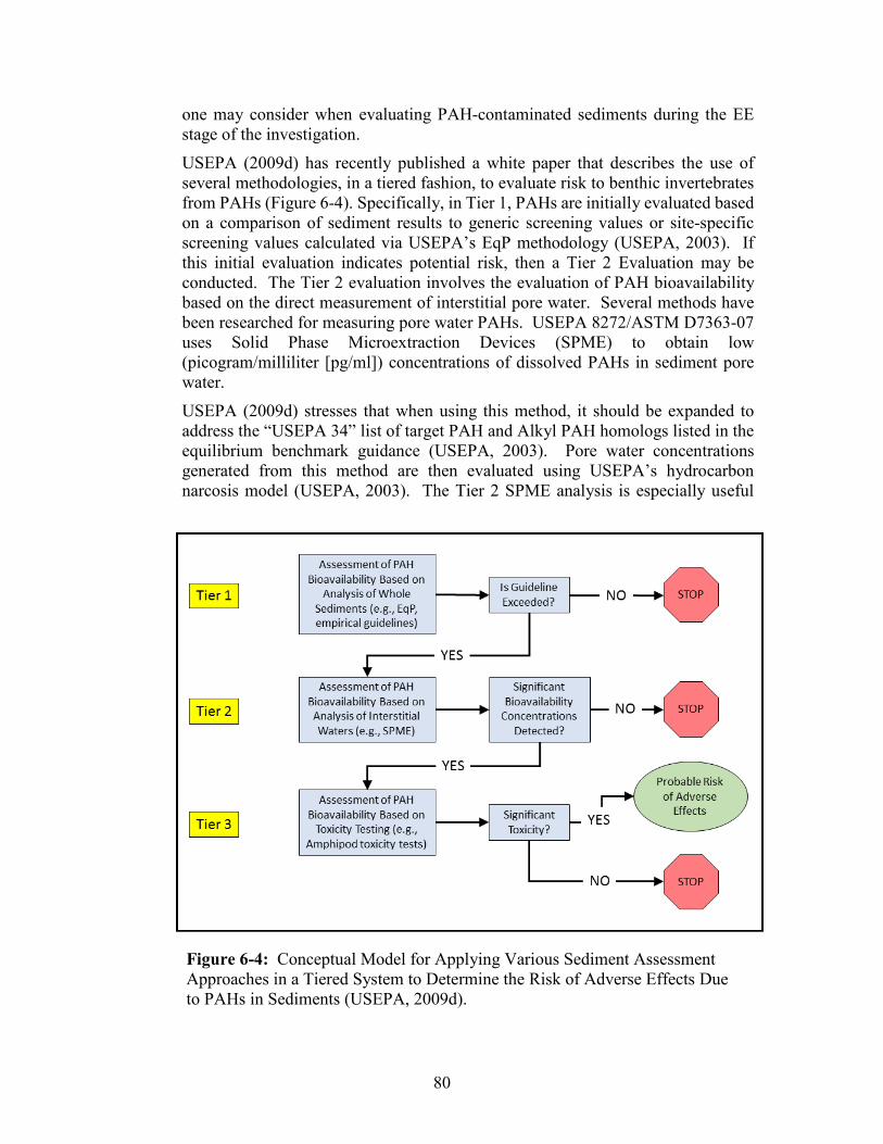
80
one may consider when evaluating PAH-contaminated sediments during the EE stage of the investigation.
USEPA (2009d) has recently published a white paper that describes the use of several methodologies, in a tiered fashion, to evaluate risk to benthic invertebrates from PAHs (Figure 6-4). Specifically, in Tier 1, PAHs are initially evaluated based on a comparison of sediment results to generic screening values or site-specific screening values calculated via USEPA’s EqP methodology (USEPA, 2003). If this initial evaluation indicates potential risk, then a Tier 2 Evaluation may be conducted. The Tier 2 evaluation involves the evaluation of PAH bioavailability based on the direct measurement of interstitial pore water. Several methods have been researched for measuring pore water PAHs. USEPA 8272/ASTM D7363-07 uses Solid Phase Microextraction Devices (SPME) to obtain low (picogram/milliliter [pg/ml]) concentrations of dissolved PAHs in sediment pore water.
USEPA (2009d) stresses that when using this method, it should be expanded to address the “USEPA 34” list of target PAH and Alkyl PAH homologs listed in the equilibrium benchmark guidance (USEPA, 2003). Pore water concentrations generated from this method are then evaluated using USEPA’s hydrocarbon narcosis model (USEPA, 2003). The Tier 2 SPME analysis is especially useful
Figure 6-4: Conceptual Model for Applying Various Sediment Assessment Approaches in a Tiered System to Determine the Risk of Adverse Effects Due to PAHs in Sediments (USEPA, 2009d).
81
when evaluating PAH-contaminated sediments in industrialized and urban settings where the presence of black soot (soot carbon), which is known to influence PAH bioavailability, is potentially present. This method was demonstrated by Hawthorne, et al. (2007) to be significantly better than conventional sediment chemistry tests, as well as EqP, for predicting impact to survival as determined by sediment toxicity tests using a sensitive sediment-dwelling species (Hyalella azteca). If Tier 2 results indicate the potential for risk, then the assessment may proceed to Tier 3 in which sediment toxicity testing is conducted in the ERA stage of the investigation (6.2.2.5).
While the USEPA tiered approach discussed above is in the form of a “white paper,” it represents a logical, step-wise approach that the investigator may use when assessing ecological risk to benthic invertebrates from PAH-contaminated sediments.
As noted above, PAHs are present as diffuse anthropogenic pollutants in many water bodies and concentrations in the low part per million (ppm) range can be expected in urban watersheds. As such, it is imperative that background area samples be collected when evaluating PAHs to establish an accurate range of PAH background contaminant levels (Section 5.3.4). This information will aid in determining if the PAHs are related to a site discharge, and may potentially influence the development of an RMD.
6.4.7 Polychlorinated Biphenyls (Aroclor vs. Congener) Polychlorinated biphenyls (PCB) are two-ringed structures with a variety of chlorination, produced originally under the trade name “Aroclor.” Aroclors are mixtures of 209 possible congeners and were produced with a range of chlorination (e.g., Aroclor 1016 was 16% chlorine by weight, whereas Aroclor 1260 was 60% chlorine by weight). PCBs may also be divided into 10 homolog classes ranging from monochlorobiphenyl to decachlorobiphenyl. Depending on the application, a variety of Aroclor mixtures (typical mixtures were Aroclor 1016, 1242, 1248, 1254, and 1260) were used and their chemical signatures are still found within environmental media (Ashley et al., 2003 and Imamoglu and Christensen, 2002). Because of physical, chemical, and biological processes, the lower molecular weight (and less chlorinated) PCBs within the mixture are less frequently found compared to relatively more stable (refractory) higher molecular weight congeners (Ashley et al., 2003 and Bernhard, et al., 2001). For example, depending on when the mixture was released into the environment, some of the 209 PCB congeners present in an original Aroclor mixture may have degraded and it is not uncommon for the mono, di, and tri-substituted PCBs to be less prevalent in environmental and biological media than the more chlorinated congeners (Ashley et al., 2003). The weathering of the original Aroclor mixtures and congeners presents some challenges to ecological risk assessors attempting to determine how best to assess potential risks posed by exposure to these chemicals (de Solla, et al., 2010).
Twelve dioxin-like PCB congeners have been identified by the World Health Organization (WHO) and assigned Toxic Equivalency Factors (TEF) because they produce biological effects similar to 2,3,7,8-TCDD with varying potencies and
82
generally act together in an additive fashion. The term “2,3,7,8-TCDD” refers to the single compound, 2,3,7,8-tetrachloro dibenzo-p-dioxin, the most toxic form of this class of compounds. Refer to Section 6.4.8 for management of PCB congener data via the Toxic Equivalency (TEQ) approach.
It is important for the field sampling and analysis plan to specify whether environmental media and biota will be analyzed for individual PCB Aroclors, homolog groups, 209 PCB congeners, or the 12 dioxin-like PCB congeners. In most cases, sampling conducted for the EE during the SI should be focused on individual PCB Aroclor analysis. Unless there is clear indication that more rigorous analyses are required, such as for a site known to have elevated PCBs in ESNRs, this approach is reasonable because analyzing samples for Aroclors is less time-consuming and less costly than conducting analyses for the homologs or the congeners (Bernhard and Petron, 2001). For screening purposes, individual PCB Aroclors may be an appropriate level of analysis, particularly where there are time and financial constraints, and where the size of the potentially impacted area is relatively small. During the remedial investigation, where the ERA, potential remedy, or source attribution depends on the speciation of the PCBs present in the samples, it may be necessary to consider the more detailed PCB congener or homolog analysis. It may be appropriate to conduct PCB congener or homolog analyses on a subset or percentage of the total samples rather than on all samples.
6.4.8 Chlorinated Dioxin, Furans, and Dioxin-like Polychlorinated Biphenyls
This section is intended to provide guidance on when a dioxin-like (polychlorinated- dioxin, furan, or biphenyl) investigation is warranted and how to perform the investigation, evaluate the data in the EE and ERA, and present results.
Polychlorinated dibenzo-p-dioxins (PCDD), polychlorinated dibenzofuran (PCDF), and polychlorinated biphenyls (PCBs) are persistent biomagnifying contaminants typically found in the environment as a mixture of congeners, all of which present similar chemical structures. There are 75 possible PCDD congeners, 135 possible PCDF congeners, and 209 possible PCB congeners. The congener pattern in a mixture will vary depending on the source material or operation that generated these compounds and their toxicity depends on the number and location of chlorine atoms. This guidance document focuses on the internationally recognized subset of the most toxic congeners (i.e., the 7 PCDD, 10 PCDF, and 12 PCB compounds) that contain laterally-substituted chlorine in the 2, 3, 7, and 8 positions for the PCDDs and PCDFs and laterally-substituted chlorines in the 3,4,5/3’,4’,5’ positions for the PCBs. To simplify the assessment of the toxicity of these complex mixtures, the USEPA adopted a WHO procedure based on the relative toxicities of the 29 individual congeners to 2,3,7,8-TCDD, for which the most toxicological information is available. This procedure is commonly referred to as the TEQ approach and was presented and described in USEPA (1987, 2008b) and Van den Berg et al. (1998, 2006). Although refinements and updates to application of this

83
procedure have occurred, the basic premise has stayed the same and continues to be used by the USEPA.
The term "dioxins" refers to the 17 tetra- through octa-chlorinated dioxin and furan and 12 tetra- through hexa-chlorinated biphenyl compounds assigned TEF values by the WHO. Dioxins and furans are formed as unintended by-products of specialty chemical processes or combustion of chlorine-containing substances. Furans and dioxin-like PCBs occur in various proportions in commercial PCBs under various trade names. These compounds are highly hydrophobic. When released into the environment, dioxins, furans and dioxin-like PCBs bind to solids and are typically found in the highest concentrations in soil or sediment. High volume water sampling of surface, ground and pore waters using EPA Methods 1613B and 1668A/B can detect and quantify these congeners in suspended solids and in the dissolved state (USEPA 1994c and 1999c). Biological matrices can be routinely characterized as well. Testing for dioxin is relatively expensive; therefore, dioxin testing is warranted only under certain site conditions. Some examples are as follows:
• when site history indicates manufacturing (e.g., synthesis, blending or storage) or application of chlorophenolic or pesticide and herbicide compounds, which are known to lead to formation of chlorinated dioxins and furans. These chemicals were identified by USEPA (1980) as Class I and II chemicals related to dioxin formation and Class I and II pesticides related to dioxin formation, respectively;
• when site history indicates bleach-kraft pulp and paper mill processes involving the use of chlorine and chlorine derivatives;
• when site history indicates PCB contamination (e.g., contaminated oils or other materials containing a high percentage of chlorine-containing substances) that may have been involved in a fire, including building interior fires;
• when site history indicates burning of plastics or other materials containing chlorine-containing compounds (e.g., burning of plastic coated wiring for precious metals recovery, miscellaneous burning of refuse with high percentage of plastic or vinyl-like materials);
• when site history indicates chlor-alkali plant manufacturing processes using carbon electrodes.
As described in Section 5.3, sampling and analysis may be conducted in a phased manner with soil samples from source areas prioritized for analysis, followed by sampling in contaminant migration pathways and ESNRs. Dioxin source areas include areas of spills, discharges, burning grounds, and ash or waste disposal. Soil and sediment sampling depth intervals are determined site-specifically; however, because dioxin binds strongly to particulate matter, it is most often found in surface or shallow depth soil and sediment intervals, and these intervals should be targeted for sampling. The exception to this is when site information indicates burial of potential dioxin-impacted soil and sediment (or ash), such as through landfilling operations, soil re-working activities on site, or long-term accretion of clean sediments. In these situations, alternate depths are targeted based on site
84
information and conditions. For fly ash or combustion waste sources, sample intervals may be guided by visual evidence of the ash.
Depending on historic site operations, best professional judgment should be used regarding the decision to limit the field sampling and analysis plan and the TEQ process to only dioxin and furans or only dioxin-like PCB congeners, or to evaluate both contaminant classes.
Detailed specifics regarding the TEQ approach can be found in Appendix I.
6.4.9 Historic Fill Material and Dredged Material Certain areas of sites and ESNRs associated with sites may have, over time, received industrial fill material or dredged materials. This practice was likely to have been more common at sites adjacent to water bodies where fill was used to create upland or to improve grade, and where low-lying areas provided for easy deposition of dredged materials. During the SI, COPECs may be found in soil, surface water, and sediment collected from these areas, yet the source of these chemicals may have little or no link to past or present site operations. The identification of historic fill and dredged materials and management options for these areas should be evaluated during the SI and RI in accordance with N.J.A.C. 7:26E–3.12, 4.7, and 5.4, and the Historic Fill Material Technical Guidance (www.nj.gov/dep/srp/guidance). These references address remedial actions in areas of historic fill for the protection of human health in upland, non-environmentally sensitive natural resource (ESNRs). Different approaches are needed for remedial investigations and remedial actions of historic fill associated with ESNRs because N.J.S.A.58:10B-12 and N.J.A.C. 7:26E requires ecological receptors to be evaluated on a case-by-case basis and because presumptive remedies may or may not be appropriate in ESNRs.
A presumptive remedy in an upland area that is not an ESNR may be implemented with or without data collection, i.e., it can be assumed that the historic fill is contaminated above human health-based Residential Soil Remediation Standards. However, because a presumptive remedy in an ESNR, such as capping, could cause a natural resource injury (see N.J.A.C. 7:26E-5.1(d)6), data-guided decisions using the ecological risk assessment/risk management process are needed. This approach is in accordance with N.J.S.A.58:10B-12h.(1), which states that there is a rebuttable presumption that the NJDEP shall not require any person to remove or treat historic fill material in order to comply with applicable health risk or environmental standards; the NJDEP may rebut the presumption only upon finding by the preponderance of the evidence that the use of engineering or institutional controls would not be effective in protecting public health, safety, and the environment. When an ESNR and historic fill are co-located, or an ESNR is impacted by historic fill, the contaminants should be investigated and evaluated for impacts to ecological receptors, similar to any other source, in accordance with N.J.A.C. 7:26E-1.16, 3.6 (b), and 4.8, with remedial decisions based on weighing environmental benefits vs. potential adverse impacts to the resource. If an unacceptable impact is determined, ecological exposure should be mitigated. However, because capping is not a presumptive remedy in an ESNR, data collection is needed in a historic fill-
85
impacted ESNR to guide remedial decisions and the risk management process (see Section 9.2), and alternative remedial measures should be considered. For example, depending on the results of the ecological risk assessment, it may or may not be appropriate to clear-cut and cap a multi-acre mature forested wetland to achieve ecological clean up goals using the data-guided risk management process, an alternate remedial measure, such as hot spot removal, should be considered to accomplish risk reduction.
If the historic fill is in an upland area that is not an ESNR, delineation of historic fill is not required beyond the property boundary. However, it is appropriate to delineate historic fill impacts in an offsite ESNR if the historic fill is not regional or if the historic fill is regional but contaminant source attribution is uncertain (i.e., possibly site related) or contaminants are aberrant qualitatively and/or quantitatively (e.g., elevated concentrations of Mercury, PCBs). Data to document consistency or disparity with regional levels are recommended. If historic fill is on a bank and leaching to an offsite water body, bank stabilization would be an example of an appropriate remedial action.
6.4.10 Acid-Volatile Sulfides/Simultaneously Extracted Metals Bioavailability and associated toxicity of some divalent metals found in anoxic sediment has been linked to the presence of acid-volatile sulfides (AVS) and their relationship to simultaneously extracted metals (SEM). The USEPA has recommended the use of the AVS/SEM ratio as a predictor of the bioavailability of these metals in sediment (USEPA, 2005b).
The AVS component of sediment is comprised of a variety of reduced sulfur compounds, quantified using a cold acid extraction. The SEM component includes the reactive metal fraction (including cadmium, copper, lead, nickel, silver, and zinc) that is extracted with the AVS. Recent literature suggests that Hg should be included with the SEM components (USEPA, 1997c).
The AVS present in sediment reacts with the SEM to form insoluble metal sulfides that are significantly less bioavailable for uptake by benthic organisms than the corresponding free metals. For divalent metals, one mole of SEM will react with one mole of AVS (although one mole of silver requires two moles of AVS). Therefore, if the total concentration of AVS is greater than the total concentration of SEM, the SEM will likely all be bound as nontoxic metal sulfides. Conversely, if the total concentration of SEM is greater than the AVS, the excess fraction of the metals may exist as bioavailable free metals that could contribute to toxicity.
Bulk sediment metals concentrations are a poor predictor of potential toxicity. The use of AVS/SEM ratios, along with organic carbon normalization has been found to be a better predictor of sediment toxicity. Earlier literature cites the ratio of ∑SEM to AVS (e.g., ∑SEM/AVS). More recent literature, however, express the difference between ∑SEM and AVS (e.g., ∑SEM-AVS). The advantages to using ∑SEM-AVS is that the ratio does not get very large when AVS is very low, and that it can be modified to develop partitioning relationships that include other phases such as TOC (Di Toro et al., 2005a,b). The use of the newer method is
86
preferred when evaluating divalent metal toxicity because it takes into account the presence of TOC on a site-specific level.
A recent study has indicated that measurement of AVS and SEM is not reproducible between laboratories (Hammerschmidt and Burton, 2010). By sending four sediment samples to each of seven independent laboratories, demonstrated that measured concentrations of both AVS and SEM were highly variable. Measurement of AVS in the four samples varied between laboratories by factors of 70 to 3,500-fold. Measurement of SEM in the four samples varied between laboratories by factors of 17 to 60-fold. As a result, the calculation of AVS/SEM ratios was highly uncertain.
The interlaboratory variation in AVS/SEM was attributed to differences in the USEPA-approved extraction methods (gravimetry, colorimetry, gas chromatographic photoionization, and ion-specific electrochemistry). Variability may also be introduced through sample heterogeneity, and through oxidation of reduced sulfur species between the times of collection and analysis. In addition, seasonal fluctuations in sediment chemistry can affect AVS/SEM measurements. A follow-up interlaboratory comparison was conducted by Brumbaugh et al. (2011) where AVS and SEM nickel concentrations were measured by five laboratories. In this study, the labs were aware of the planned interlaboratory comparison and they were provided guidance for conducting sample preparation, analysis, and quality control measurements. The results of this study showed that measurements of AVS and SEM-AVS can be reproducible among laboratories, thus emphasizing the need for consistent quality control procedures.
While AVS/SEM is a potentially useful tool for assessing bioavailability and associated toxicity of sediment metals, it should not be used as a stand-alone line of evidence for evaluating risk until laboratory methods have been standardized to allow consistent interlaboratory reproducibility.
6.4.11 Guidance for the Evaluation of Mercury Contaminated Sites Some contaminants found at sites may require additional evaluation due to their toxicological and environmental fate profiles. One of these contaminants is mercury which has been found at a variety of contaminated sites in the US and elsewhere (Harris 2008, Randall and Chattopadhyay 2013). There are various chemical forms of mercury, each of which has a different toxicological and fate profile. In addition, mercury can be transformed by microbes from an inorganic form to methyl mercury, a more toxic and bio-accumulative species (Zhang, Kim et al. 2012). The ability of methyl mercury to bio-accumulate through aquatic and terrestrial food webs has been known for many years (Jardine, Kidd et al. 2013), and this knowledge base can be applied when mercury (inorganic and organic) is found at contaminated sites in New Jersey. The additional evaluation of mercury sites may include food-chain modeling of the potential movement of mercury through a food web at or adjacent to the site under study, or collecting food / prey to determine where mercury is entering the aquatic and terrestrial food web. Of recent note is the finding that mercury in the aquatic compartment can be transferred to the terrestrial environment and that may also be an additional

87
consideration during the site investigation and risk assessment process (Cristol, Brasso et al. 2008).
7.0 Determination of Ecological Risk-Based Remediation Goals The output of the risk characterization process (Section 6.1.3 et. seq.) determines whether remedial goals need to be determined for given ecological receptor-COPEC pairs (as illustrated in Figure 7-1, below). Ecological remediation goals can be the ESC (or appropriate background levels as per Section 5.3.4) or can be site-specific risk-based goals, which are determined from biological test data collected in accordance with Section 6.0. They are considered preliminary because adjustments may be made following the RMD process (Section 9.0). These numeric goals are delineation criteria and target post-remedial concentrations. Remediation goals should be determined for all COPECs in any exposure pathway where risk is elevated using various lines of evidence such as food chain modeling and soil and sediment toxicity test results (See Figure 7-1). All ecological risk-based remediation goals must be approved by NJDEP (N.J.A.C. 7:26E-4.8(c)3).
Exposure pathway HQ >1 in ERA dietary Protective soil concentrations, mg/kg (receptor) exposure models or (see Figures 7-2 and 7-3 for calculations) statistically significant toxicity Avian Insectivore PCBs 2.8 (Woodcock) Mercury 2.4 Lead 320 Copper 402 Mammalian Herbivore Lead 760 (Muskrat) Copper 1,600 Soil Invertebrate Lead 420 Community Copper 290 (site-specific AET)
For PCBs and mercury, since risk is indicated only for avian insectivores, the remediation goals are 2.8 mg/kg and 2.4 mg/kg respectively. For lead and copper, it is recommended that the most conservative concentration be selected as the remediation goal, (i.e., 320 mg/kg for lead based on risk to avian insectivores and 290 mg/kg for copper based on soil toxicity to the soil invertebrates).
Figure 7-1. Hypothetical Example of Media Concentrations to Consider for Selection of Ecological Risk-Based Remediation Goals.
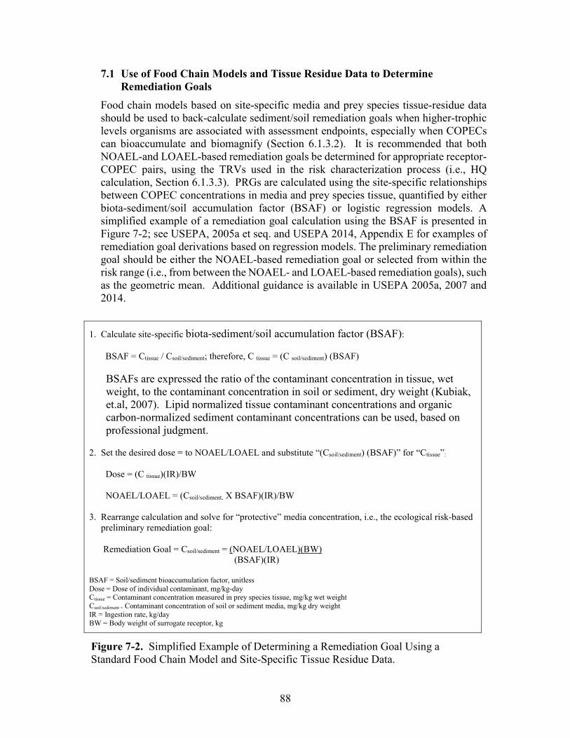
88
7.1 Use of Food Chain Models and Tissue Residue Data to Determine Remediation Goals
Food chain models based on site-specific media and prey species tissue-residue data should be used to back-calculate sediment/soil remediation goals when higher-trophic levels organisms are associated with assessment endpoints, especially when COPECs can bioaccumulate and biomagnify (Section 6.1.3.2). It is recommended that both NOAEL-and LOAEL-based remediation goals be determined for appropriate receptor-COPEC pairs, using the TRVs used in the risk characterization process (i.e., HQ calculation, Section 6.1.3.3). PRGs are calculated using the site-specific relationships between COPEC concentrations in media and prey species tissue, quantified by either biota-sediment/soil accumulation factor (BSAF) or logistic regression models. A simplified example of a remediation goal calculation using the BSAF is presented in Figure 7-2; see USEPA, 2005a et seq. and USEPA 2014, Appendix E for examples of remediation goal derivations based on regression models. The preliminary remediation goal should be either the NOAEL-based remediation goal or selected from within the risk range (i.e., from between the NOAEL- and LOAEL-based remediation goals), such as the geometric mean. Additional guidance is available in USEPA 2005a, 2007 and 2014.
1. Calculate site-specific biota-sediment/soil accumulation factor (BSAF): BSAF = Ctissue / Csoil/sediment; therefore, C tissue = (C soil/sediment) (BSAF)
BSAFs are expressed the ratio of the contaminant concentration in tissue, wet weight, to the contaminant concentration in soil or sediment, dry weight (Kubiak, et.al, 2007). Lipid normalized tissue contaminant concentrations and organic carbon-normalized sediment contaminant concentrations can be used, based on professional judgment.
2. Set the desired dose = to NOAEL/LOAEL and substitute “(Csoil/sediment) (BSAF)” for “Ctissue”:
Dose = (C tissue)(IR)/BW NOAEL/LOAEL = (Csoil/sediment, X BSAF)(IR)/BW 3. Rearrange calculation and solve for “protective” media concentration, i.e., the ecological risk-based
preliminary remediation goal: Remediation Goal = Csoil/sediment = (NOAEL/LOAEL)(BW) (BSAF)(IR) BSAF = Soil/sediment bioaccumulation factor, unitless Dose = Dose of individual contaminant, mg/kg-day Ctissue = Contaminant concentration measured in prey species tissue, mg/kg wet weight Csoil/sediment = Contaminant concentration of soil or sediment media, mg/kg dry weight IR = Ingestion rate, kg/day BW = Body weight of surrogate receptor, kg
Figure 7-2. Simplified Example of Determining a Remediation Goal Using a Standard Food Chain Model and Site-Specific Tissue Residue Data.
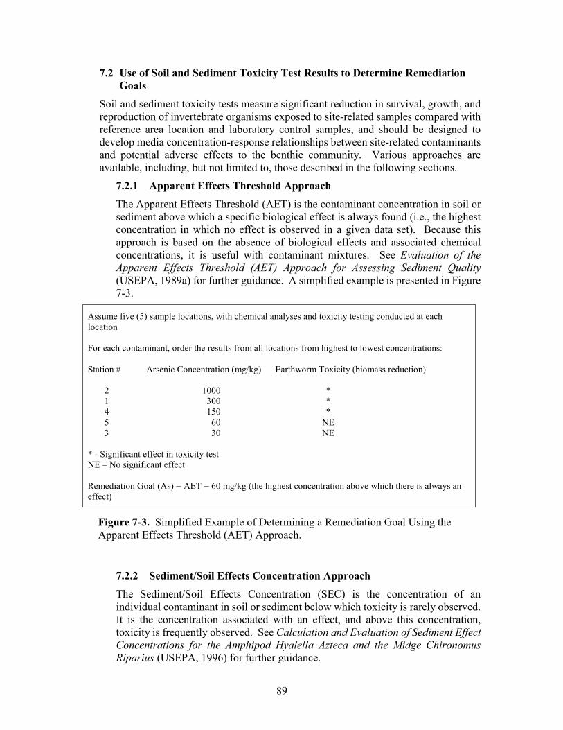
89
7.2 Use of Soil and Sediment Toxicity Test Results to Determine Remediation Goals
Soil and sediment toxicity tests measure significant reduction in survival, growth, and reproduction of invertebrate organisms exposed to site-related samples compared with reference area location and laboratory control samples, and should be designed to develop media concentration-response relationships between site-related contaminants and potential adverse effects to the benthic community. Various approaches are available, including, but not limited to, those described in the following sections.
7.2.1 Apparent Effects Threshold Approach The Apparent Effects Threshold (AET) is the contaminant concentration in soil or sediment above which a specific biological effect is always found (i.e., the highest concentration in which no effect is observed in a given data set). Because this approach is based on the absence of biological effects and associated chemical concentrations, it is useful with contaminant mixtures. See Evaluation of the Apparent Effects Threshold (AET) Approach for Assessing Sediment Quality (USEPA, 1989a) for further guidance. A simplified example is presented in Figure 7-3.
Assume five (5) sample locations, with chemical analyses and toxicity testing conducted at each location For each contaminant, order the results from all locations from highest to lowest concentrations: Station # Arsenic Concentration (mg/kg) Earthworm Toxicity (biomass reduction) 2 1000 * 1 300 * 4 150 * 5 60 NE 3 30 NE * - Significant effect in toxicity test NE – No significant effect Remediation Goal (As) = AET = 60 mg/kg (the highest concentration above which there is always an effect)
7.2.2 Sediment/Soil Effects Concentration Approach The Sediment/Soil Effects Concentration (SEC) is the concentration of an individual contaminant in soil or sediment below which toxicity is rarely observed. It is the concentration associated with an effect, and above this concentration, toxicity is frequently observed. See Calculation and Evaluation of Sediment Effect Concentrations for the Amphipod Hyalella Azteca and the Midge Chironomus Riparius (USEPA, 1996) for further guidance.
Figure 7-3. Simplified Example of Determining a Remediation Goal Using the Apparent Effects Threshold (AET) Approach.
90
7.3 Application of Ecological Remediation Goals The need for a remedial action in an ESNR is determined by comparing the selected ecological remediation goal (ESC/background or site-specific ecological risk-based remediation goal) to soil/sediment COPEC concentrations. The extent of remediation needs to address the area that exceeds the remediation goals, and additional factors including, but not limited to: the biotic zone; whether the sediment/soil contaminant mass outside of the biotic zone is a continuing source; whether deeper sediment/soil could become exposed in the future; and the potential for biomagnification.
8.0 Uncertainty Several sources of uncertainty are associated with ecological risk estimates. These include initial selection of COPECs based on the sampling data, estimates of toxicity to ecological receptors based on limited laboratory data (usually on other species), and uncertainties in exposure and effects assessment. As part of the final steps in estimating potential ecological risks associated with a site, the magnitude of uncertainties associated with the risk estimation should be discussed.
Uncertainty in risk estimation has both qualitative and quantitative components. Qualitative uncertainty analyses are recommended by guidance (USEPA, 1988) and contribute to the confidence with which risk assessment conclusions can be drawn and applied (USEPA, 1989b, 1989c, and 1999a). Quantitative uncertainty analyses provide objective measures of the relative confidence in the conclusions that have been drawn in an evaluation.
Uncertainty surrounding risk assessment conclusions has important implications for risk management (USEPA, 1988, 1998a). However, uncertainty is not a single, generally applicable parameter. Uncertainty surrounding a risk estimate or application has a number of components, including parameter variability, calculation error and simplification, and the underlying reality of exposure assumptions and pathways (USEPA, 1988). Uncertainty includes both real variation (reflecting actual, mechanistic biological response ranges and variability in ecosystem conditions) and error (USEPA, 1997a).
Because biological systems are inherently uncertain and variable, some component of variability in risk estimation is due to a realistic expression of ecological conditions, while another component is due to error or uncertainty introduced by the overall analytical process. Error is the component to be minimized because error encompasses undesirable uncertainty that has been introduced by the assessment process. However, it is critically important to understand ecosystem variability because this represents an important component of the ecosystem within which RMDs will be made. Substantial differences exist between observations and conclusions made at the individual, population, and community levels of biological organization. For example, effects not manifested at the population or community levels (e.g., mortality of only a few individuals) may not be observable with the type of studies implemented. The ramifications of this also include an understanding that, because the assessment level endpoints are protective of populations
91
and communities and not individuals, the projected loss of a few individuals may not cause impacts that are important at the levels of assessment at which RMDs are made.
Because of the many potential receptor species and general lack of knowledge regarding their life cycles, feeding habits, nutritional requirements (e.g., essential elements such as arsenic, trivalent chromium, selenium, and zinc), and relative toxicological sensitivity, the uncertainty surrounding estimates of ecological risks may be substantially greater than those associated with human health risk assessment. The generic screening and regulatory criteria and TRVs used in this assessment are intended to provide conservative benchmarks, but it is important to note that no one approach to criterion or TRV derivation is adequate for all sites and all COPECs. The criteria or TRVs used in this assessment are all chemical-specific and as such, cannot address the additive, antagonistic, or synergistic effects of the chemical mixtures typically found in the environment. Further, these criteria or TRVs do not take into account the structure and dynamics of the ecosystem present at the site, site-specific conditions regulating chemical contact and bioavailability, the potential toxicity of other constituents that were not quantified, or the pervasive influence of physical stressors associated with the disruption by human activities that is characteristic of an area that may have an industrial history.
The uncertainty evaluations should be performed within a range of conditions defined by characteristics of the environment at the time field data were gathered. As such, data obtained and conclusions drawn represent a series of snapshots of site conditions and, while they can be extrapolated to a broad range of conditions, they are most accurate when site conditions are most similar to those that existed at the time of sampling. In addition, screening criteria do not necessarily reflect the entire range of possible site conditions and, as such, the applicability of conclusions is also restricted by these simplifications.
The investigator is referred to Suter et al. 2000 for a comprehensive discussion on uncertainty and the methods for calculating it.
9.0 Risk Management Considerations Decisions about whether estimated ecological risks are unacceptable and how to manage them require consideration of the magnitude of the estimated risk and the weighing of expected benefits against the expected short- or long-term harm that might be caused by the proposed action. Risk Management Decisions (RMDs) are made in a process not driven wholly by technical information even though the potential for ecological risk is a major component of the decision making. RMDs cannot be performed until ERA has been completed and ecological-based risk goals have been calculated. Overviews of ecological risk management can be found in Pittinger et al., 2001a; Pittinger et al., 2001b; Stahl et al., 2001; Wentsel et al., 2001; and USEPA, 1997a.
9.1 Soil Remediation Standards and Deed Notices Remediation to the Soil Remediation Standards (SRS) found at N.J.A.C. 7:26D - Remediation Standards is not appropriate in ESNRs because the SRS are based on human health and assume human exposure in a residential or industrial setting. Human exposure to contaminated media within an ESNR would not be expected at the same exposure level as in a residential or industrial setting. Human exposure to media in
92
ESNRs is generally limited, while exposure to ecological receptors is of greater concern. ESNRs that consist of uplands where future use may change may require a deed notice as the intention of a deed notice is the protection of public health in the event of a change in site use. Deed notices contain written notice to current and future property owners of post-remedial contaminants that will remain at a site above SRS, including when engineering controls are used to mitigate human exposure. Therefore, when the site-specific ecological risk-based remediation goals are achieved via site remediation, the appropriate receptors are protected and the need for deed notices and engineering controls, which require costly permitting and biennial certifications, is negated for most ESNRs. This approach is appropriate in areas designated as preserved in perpetuity (e.g., conservation easements, farmland preserved areas, wetland mitigation areas protected pursuant to N.J.A.C. 7:7A-15.14), because future development is restricted. However, where no such restrictions exist and where there is the potential for future development (e.g., ESNRs that may be developed into residential use [not preserved in perpetuity], or where the soil or sediment from ESNRs may be used as fill on another site), a deed notice will be required.
9.2 Risk Management Decisions The approach to setting potential remediation goals has been described in Section 7.0. RMDs involve adjusting ecological risk-based remediation goals for remedial decision making and implementation. RMDs should reduce ecological risks to levels that will result in the recovery and maintenance of healthy local populations and communities. In some instances, the proposed remedy may cause more ecological damage then leaving the contaminant in place, particularly where rare or sensitive habitats exist because of widespread physical destruction or alteration of the habitat through excavation or in situ treatment; however, leaving persistent and/or bioaccumulative contaminants in place may cause an ongoing source of contaminant exposure (USEPA, 1999a). In addition, the proposed remedial action may not be achievable because of technical impracticability.
RMDs consider the present and predicted value of the affected ESNRs, and the beneficial and detrimental effects on the ESNRs’ value with implementation of the potential remedial activities. The key components to consider during the RMD are (1) that impaired habitats can provide some valuable ecological benefit (e.g., food source, breeding, rearing, and shelter), (2) the ecosystem extends beyond the perimeter of the impaired area, and (3) reduction in ecological benefits in one area of the ecosystem may be offset by a corresponding increase in ecological benefits in another part of the ecosystem. Restoration activities should exceed the future decreased ecological benefits associated with the continued exposure to COPECs or any remedial activities. All RMDs must be approved by NJDEP (N.J.A.C. 7:26E-4.8(c)3). Examples of RMDs are noted in the following text.
The following is presented solely to serve as an example of one project’s balancing of remedial actions and preservation of habitat. Other methods of balancing these goals may be used on a site-specific basis.
A firing range is located within a 100-acre mature forested wetland, which is contiguous with another 500 acres of forested wetland, emergent wetland and upland
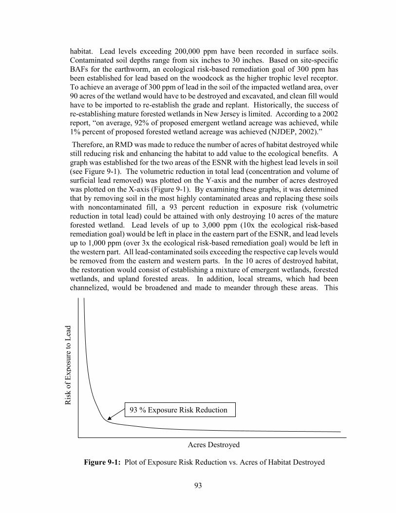
93
habitat. Lead levels exceeding 200,000 ppm have been recorded in surface soils. Contaminated soil depths range from six inches to 30 inches. Based on site-specific BAFs for the earthworm, an ecological risk-based remediation goal of 300 ppm has been established for lead based on the woodcock as the higher trophic level receptor. To achieve an average of 300 ppm of lead in the soil of the impacted wetland area, over 90 acres of the wetland would have to be destroyed and excavated, and clean fill would have to be imported to re-establish the grade and replant. Historically, the success of re-establishing mature forested wetlands in New Jersey is limited. According to a 2002 report, “on average, 92% of proposed emergent wetland acreage was achieved, while 1% percent of proposed forested wetland acreage was achieved (NJDEP, 2002).”
Therefore, an RMD was made to reduce the number of acres of habitat destroyed while still reducing risk and enhancing the habitat to add value to the ecological benefits. A graph was established for the two areas of the ESNR with the highest lead levels in soil (see Figure 9-1). The volumetric reduction in total lead (concentration and volume of surficial lead removed) was plotted on the Y-axis and the number of acres destroyed was plotted on the X-axis (Figure 9-1). By examining these graphs, it was determined that by removing soil in the most highly contaminated areas and replacing these soils with noncontaminated fill, a 93 percent reduction in exposure risk (volumetric reduction in total lead) could be attained with only destroying 10 acres of the mature forested wetland. Lead levels of up to 3,000 ppm (10x the ecological risk-based remediation goal) would be left in place in the eastern part of the ESNR, and lead levels up to 1,000 ppm (over 3x the ecological risk-based remediation goal) would be left in the western part. All lead-contaminated soils exceeding the respective cap levels would be removed from the eastern and western parts. In the 10 acres of destroyed habitat, the restoration would consist of establishing a mixture of emergent wetlands, forested wetlands, and upland forested areas. In addition, local streams, which had been channelized, would be broadened and made to meander through these areas. This
Acres Destroyed
93 % Exposure Risk Reduction
Ris
k of
Exp
osur
e to
Lea
d
Figure 9-1: Plot of Exposure Risk Reduction vs. Acres of Habitat Destroyed
94
restoration plan increased the value of the habitat while reducing the overall risk of exposure to receptors by 93 percent even though the overall average lead level in soil for the impacted area remained above the calculated ecological risk-based remediation goal.
RMDs frequently involve the decision to remove or preserve mature trees, especially in wooded wetlands. To facilitate such decisions, a standard tree survey should be conducted within the area of the preliminary remediation footprint (i.e., based on achievement of the ecological risk-based remediation goals). Trees greater than 6-8” diameter at breast height (dbh) should be indicated on a figure, coded with gps coordinates, species, and dbh. Then an assessment of ecological benefit of soil remediation vs. potential detriment of removing trees can be made. In addition to considering contaminant class, concentrations, and depth, considerations for each tree include tree size, (dbh); wildlife resting/nesting cover provided; food provided (e.g., nut, berry-bearing); canopy cover provided (e.g., canopy may help shade new restoration plantings); desirable canopy that may expand if lesser valued trees are removed; erosion control provided (e.g., near surface water bodies); presence of diseased or dead trees, or trees near the end of their natural life; access needs for heavy equipment/ability to use small excavation equipment.
10.0 Quality Assurance/Quality Control and Data Usability Analytical data collected during the EE and ERA should be of the correct nature, quality, and quantity to fulfill their intended use in remedial decision making for ESNRs. Toward this end, data quality assurance and quality control (QA/QC), data validation, and data usability assessment procedures are integral components of the field sampling, laboratory analysis, and data evaluation stages of the ecological investigation. A project-specific Quality Assurance Project Plan (QAPP) is required pursuant to N.J.A.C. 7:26E to ensure that environmental measurement tasks are appropriately planned, documented, and executed so that the resultant data are of known quality, verifiable, and defensible. The QAPP should establish data quality objectives (DQOs) and all data collected should be vetted against the DQOs prior to use. Note the term “validation” typically refers to chemical data; for nonchemical data, such as benthic community data, toxicity test data, etc., the term data “verification” may be more appropriate and these metrics should be specified in the QAPP.
The primary guidance on general QA/QA measures, QAPP preparation, DQO determination, data validation protocol, and data usability assessments is NJDEP’s Quality Assurance/Quality Control Technical Guidance. Additional information is available from various sources, including, but not limited to, those listed below:
• General - QA/QC guidance that specifically includes biological data can be found in USEPA (1997a), Appendix B, Section 4.0 and USEPA (2000a), Section 8.0. QA/QC requirements for toxicity testing are addressed in Sections 6.2.2.5 and 6.2.2.6 of this guidance.
• QAPPs - refer to USEPA (2005c) Uniform Federal Policy for Quality Assurance Project Plans. Evaluating, Assessing, and Documenting Environmental Data Collection and Use Programs. Part 1: UFP-QAPP Manual. Final Version 1.
95
• DQOs - refer to USEPA (2006b) Guidance on Systematic Planning Using the Data Quality Objectives Process. Additional information is available in USEPA (2004, 2005c, and 2006c).
• Data Validation - refer to USEPA (2002g) Guidance on Environmental Data Verification and Data Validation. Numerous additional guidance documents can be found under “Quality Assurance Guidance/RCRA and CERCLA Field and Data Validation Standard Operating Procedures (SOPs).”
• Data Usability - refer to USEPA (1992c) Guidance for Data Useability in Risk Assessment (Part A).
11.0 References Adamus, P. R., E. J. Clairain, R. D. Smith, and R. E. Young. 1987. Wetland Evaluation Technique (WET), Vol. II: Methodology (Operational draft). Washington, D.C.: Wetlands Research Program, U.S. Army Corps of Engineers, Environmental Laboratory.
Arnold, R.E. and Hodson, M.E. 2007. Effect of time and mode of depuration on tissue copper concentrations of the earthworms Eisenia andrei, Lumbricus rubellus and Lumbricus terrestris. Environmental Pollution, volume 148, number 1, pp 21-30.
Ashley, J.T.F., Horwitz, R., Steinbacher, J.C., Ruppel, B. 2003. A comparison of congeneric patterns in American eels and striped bass from the Hudson and Delaware River estuaries. Mar. Pollut. Bull. 46, 1294-1308.
ASTM (American Society for Testing and Materials). 2000. E 1391 -94 Standard guide for collection, storage, characterization, and manipulation of sediments for toxicological testing. p. 768-788. In: 2000 ASTM Standards on Environmental Sampling, Vol. 11.05 Conshohocken, PA.
ASTM (American Society for Testing and Materials). 2004. Standard Guide for Conducting Laboratory Soil Toxicity or Bioaccumulation Tests with the Lumbricid Earthworm Eisenia Fetida and the Enchytraeid Potworm Enchytraeus albidus. E1676-04. ASTM, West Conshohocken, PA.
ASTM (American Society for Testing and Materials). 2010. Standard Test Method for Measuring the Toxicity of Sediment-Associated Contaminants with Freshwater Invertebrates. E1706 - 05(2010). ASTM, West Conshohocken, PA.
ASTM (American Society for Testing and Materials). 2005b. Standard Guide Conducting Early Life-Stage Toxicity Tests with Fishes. E1241-05. ASTM, West Conshohocken, PA.
ASTM (American Society for Testing and Materials). 2007a. Standard Guide for Conducting In-situ Field Bioassays with Caged Bivalves. E2122-02(2007). ASTM, West Conshohocken, PA.
ASTM (American Society for Testing and Materials). 2007b. Standard Guide for Conducting Sediment Toxicity Tests with Polychaetous Annelids. E1611-00(2007). ASTM, West Conshohocken, PA.
96
ASTM (American Society for Testing and Materials). 2008a. Standard Test Method for Measuring the Toxicity of Sediment-Associated Contaminants with Estuarine and Marine Invertebrates. E1367-03(2008). ASTM, West Conshohocken, PA.
ASTM (American Society for Testing and Materials). 2008b. ASTM E1525-02(2008) Standard Guide for Designing Biological Tests with Sediments. ASTM, West Conshohocken, PA.
ASTM (American Society for Testing and Materials). 2009. Standard Guide for Conducting Terrestrial Plant Toxicity Tests. E1963-09. ASTM, West Conshohocken, PA.
ASTM (American Society for Testing and Materials). 2010. Standard Guide for Determination of the Bioaccumulation of Sediment-Associated Contaminants by Benthic Invertebrates. E1688-10. ASTM, West Conshohocken, PA.
Barnthouse L.W., Munns W.R., and Sorensen M.T. 2008. Population-Level Ecological Risk Assessment. Boca Raton, Florida: CRC Press. 1-337 pp.
Bartoldus, C. C. 1999. A Comprehensive Review of Wetland Assessment Procedures: A Guide for Wetland Practitioners. St. Michaels, Md.: Environmental Concern, Inc.
Bartoldus, C.C., E. W. Garbisch, and M.L. Kraus. 1994. Evaluation for Planned Wetlands (EPW): A Procedure for Assessing Wetland Functions and a Guide to Functional Design. St. Michaels, MD: Environmental Concern Inc.
Barton A.L., Stahl R.G., Bachman R., Clark J.R., deFur P.L., Ells S.J., Pittinger C.A., Slimak M.W., and Wentsel R.S. 2001. Deciding what resources to protect and setting objectives. Risk Management: Ecological risk-based decision making. Pensacola, Florida: SETAC Press. pp. 41-56.
Bernhard, T. and Petron, S. 4/9/2001. Analysis of PCB Congeners vs. Aroclors in Ecological Risk Assessment. (7 p.) http://www.clu-in.org/download/contaminantfocus/pcb/analysis-of-pcb-congeners.pdf
Bonham, C.D. 1989. Measurements for Terrestrial Vegetation. John Wiley & Sons, NY.
Bowers, T.S., N. Shifrin and B. Murphy. 1996. Statistical Approach to Meeting Soil Cleanup Goals, Environ. Sci. Technol., Vol. 30, pp. 1437-1444, 1996.
Braun, C. 2005. Techniques for Wildlife Investigations and Management. The Wildlife Society, Bethesda, MD.
Breden, T.F. 1989. A Preliminary Natural Community Classification of New Jersey. in E.F. Karlin. New Jersey’s Rate and Endangered Plants and Animals. Institute for Environmental Studies, Ramapo College, Mahway, NJ.
Brinson, M. M. 1993. A Hydrogeomorphic Classification for Wetlands. Wetlands Research Program Technical Report WRP-DE-4.
Brumbaugh, W.G., Hammerschmidt, C.R., Zanella, L., Rogevich, E., Salata, G. and Bolek, R. 2011. Interlaboratory Comparison of Measurements of Acid-Volatile Sulfide and Simultaneously Extracted Nickel in Spiked Sediments, Environmental Toxicology & Chemistry, 30(6): 1306-1309, (91856).
97
Burton, G.A. Jr, Greenberg, M.S., Rowland, C.D., Irvine, C.A., Lavoie, D.R., Brooker, J.A., Moore, L., Raymer, D.F.N. and McWilliam, R.A. 2004. In situ exposures using caged organisms: a multi-compartment approach to detect aquatic toxicity and bioaccumulation. Environmental Pollution, volume 134, number 1, pp. 133-144.
Canadian Council of Ministers of the Environment. 1999. Protocol for the Derivation of Canadian Tissue Residue Guidelines for the Protection of Wildlife that Consume Aquatic Biota. http://www.ccme.ca/assets/pdf/trg_protocol.pdf.
Chadwick, D., Groves, J. Harre, B. Paulsen, R. and Smith, C. 2003. Coastal Contaminant Migration Monitoring: The Trident Probe and Ultraseep System: Hardware Description, Protocols, and Procedures. SSC San Diego Technical Report 1902. http://oai.dtic.mil/oai/oai?verb=getRecord&metadataPrefix=html&identifier=ADA416834.
Chadwick, B., and Hawkins, A. 2008. Monitoring of Water and Contaminant Migration at the Groundwater-Surface Water Interface. ER200422 Final Report. Arlington, Va. U.S. Department of Defense, Environmental Security and Technology Certification Program. www.dtic.mil/cgi-bin/GetTRDoc?AD=ADA607246.
Collins, B. R. and Anderson, K.H. 1994. Plant Communities of New Jersey. Rutgers University Press, New Brunswick, NJ.
Cristol, D. A., R. L. Brasso, A. M. Condon, R. E. Fovargue, S. L. Friedman, K. K. Hallinger, A. P. Monroe and A. E. White (2008). "The movement of aquatic mercury through terrestrial food webs." Science 320: 325.
Davis, D.E. 1982. CRC Handbook of Census Methods for Terrestrial Vertebrates. CRC Press, Boca Raton, FL.
Davison, W., Fones, G., Harper, M., Teasdale, P., and Zhang H. 2000. Dialysis, DET and DGT: In Situ Diffusional Techniques for Studying Water, Sediment and Soils, pp. 495−569 in In Situ Monitoring of Aquatic Systems: Chemical Analysis and Speciation, J. Buffle and G. Horvai, eds. NY: Wiley.
de Solla, S.R., Weseloh, D.V., Hebert, C.E., and Pekarik C. 2010. Impact of changes in analytical techniques for the measurement of polychlorinated biphenyls and organochlorine pesticides on temporal trends in herring gull eggs. Environmental Toxicology and Chemistry, v29, n7, p1476-1483, July 2010 http://onlinelibrary.wiley.com/doi/10.1002/etc.191/pdf
Di Toro, D. M., Zarba, C. S., Hansen, D. J., Berry, W. J., Swartz, R. C., Cowan, C. E., Pavlou, S. P., Allen, H. E., Thomas, N. A., and Paquin, P. R. 1991. Technical Basis for Establishing Sediment Quality Criteria for Nonionic Organic Chemicals Using Equilibrium Partitioning, Environmental Toxicology and Chemistry 10: 1541-83.
Di Toro D. M., Berry, W. J., Burgess, R. M., Mount, D. R., O’Connor, T. P., and Swartz, R. C. 2005a. The Predictive Ability of Sediment Quality Guidelines Derived Using Equilibrium Partitioning, in Use of Sediment Quality Guidelines and Related Tools for the Assessment of Contaminated Sediments, R. J. Wenning, G. Bartley, C. Ingersoll, and D. Moore, eds. Pensacola, FL.: SETAC Press.
98
Di Toro, D. M, Mcgrath, J. M., Hansen, D. J., Berry, W. J., Paquin, P. R., Mathew, R., Wu, K. B., and Santore, R. C. 2005b. Predicting Sediment Metal Toxicity Using a Sediment Biotic Ligand Model: Methodology and Initial Application, Environmental Toxicology and Chemistry 24(10): 2410–27.
Di Toro, D. M. 2008. Bioavailability of Chemicals in Sediments and Soils: Toxicological and Chemical Interactions, pp. B-73-B-103 in SERDP and ESTCP Expert Panel Workshop on Research and Development Needs for Understanding and Assessing the Bioavailability of Contaminants in Soils and Sediments. Washington, DC. Strategic Environmental Research and Development Program and the Environmental Security Technology Certification Program. http://serdp-estcp.org/content/download/8049/99405/version/1/file/Bioavailability_Wkshp_Nov_2008.pdf.
Duncan, P., Greenberg, M., Leja, S., Williams, J., Black, C., Henry, R., and Wilhelm, L. 2007a. Case Study of Contaminated Groundwater Discharge: How In Situ Tools Link an Evolving Conceptual Site Model with Management Decisions, Integrated Environmental Assessment and Management 3: 279–89.
Duncan, P., Henry, R., Sheldrake, S., and Thompson, D. 2007b. Adaptation of Groundwater Evaluation and Sampling Tools for Underwater Deployment, pp. 55–83 in Diving for Science 2006, Proceedings, American Academy of Underwater Sciences 25th Symposium, Dauphin Island, AL., J. M. Godfrey and N. W. Pollock, eds. https://archive.epa.gov/region10/diving/web/pdf/duncan_etal_groundwater_eval_tools_aaus_2006-2.pdf.
Efroymson, R.A., Sample, B.E., and Peterson, M.J. 2004. Ecotoxicity Test Data for Total Petroleum Hydrocarbons in Soil: Plants and Soil-Dwelling Invertebrates. Human and Ecological Risk Assessment, 10: 207-231.
Eisler, R. 2000. Handbook of Chemical Risk Assessment - Health Hazards to Humans, Plants, and Animals. Volume 2 Organics. Chapter 25 PAHs. Boca Raton: Lewis Publishers.
Environment Canada. 1994. Guidance document on collection and preparation of sediments for physicochemical characterization and biological testing. Environmental Protection Series. Report EPS 1/RM/29, December 1994, 132 pp.
Federal Interagency Committee for Wetland Delineation. 1989. Federal Manual for Identifying and Delineating Jurisdictional Wetlands. USACE, USEPA, USFWS, and USDA Soil Conservation Service, Washington, DC. Cooperative technical publication. 76 pp. plus appendices.
Hammerschmidt, C.R. and Burton, G.A., Jr. 2010. Measurements of Acid Volatile Sulfide and Simultaneously Extracted Metals are Irreproducible Among Laboratories. Environmental Technology and Chemistry, Volume 29, number 7, pp. 1453-1456.
Hansen, D.J., Berry, W.J., Mahony, J.D., Boothman, W.S., Di Toro, D.M., Robson, D.L., Ankley, G.T., Ma, D., Yan, Q., and Pesch, C.E. 1996. Predicting the Toxicity of Metal-Contaminated Field Sediments Using Interstitial Concentration of Metals and Acid-
http://serdp-estcp.org/content/download/8049/99405/version/1/file/Bioavailability_Wkshp_Nov_2008.pdf
http://serdp-estcp.org/content/download/8049/99405/version/1/file/Bioavailability_Wkshp_Nov_2008.pdf
99
Volatile Sulfide Normalizations, Environmental Toxicology and Chemistry 15(12): 2080–94.
Harris, R. K., David; Mason, Richard; Murray, Michael W.; Reash, Robin; Saltman, Tamara (2008). Introduction. Ecosystem responses to mercury contamination. Indicators of change. R. K. Harris, David P.; Mason, Robert; Murray, Michael W.; Reash, Robin; Saltman, Tamara. Boca Raton, Florida, CRC Press: 1-13.
Harshberger, J.W. 1970. The Vegetation of the New Jersey Pine-Barrens. Dover Publications, NY.
Hawthorne, S.B., Azzolina, N.A., Neuhauser, E.F., Kreitinger, J.P. 2007. Predicting Bioavailability of Sediment Polycyclic Aromatic Hydrocarbons to Hyalella azteca using Equilibrium Partitioning, Supercritical Fluid Extraction, and Pore Water Concentrations. Environ. Sci. Technol. 2007, 41, 6297–6304.
Imamoglu, I., Li, K., and Christensen, E.R. 2002. PCB sources and degradation in sediments of Ashtabula River, USA, determined from receptor models. Water Science and Technology, 46(3), p.89-96.
ITRC (Interstate Technology & Regulatory Council). 2005. Technology Overview of Passive Sampler Technologies. DSP-4. Washington, DC.: Interstate Technology & Regulatory Council, Authoring Team. www.itrcweb.org.
ITRC (Interstate Technology & Regulatory Council). 2011. Incorporating Bioavailability Considerations into the Evaluation of Contaminated Sediment Sites. CS-1. Washington, DC.: Interstate Technology & Regulatory Council, Contaminated Sediments Team. http://www.itrcweb.org/contseds-bioavailability/.
Jardine, T. D., K. A. Kidd and N. O'Driscoll (2013). "Food web analysis reveals effects of pH on mercury bioaccumulation at multiple trophic levels in streams." Aquatic Toxicology 132-133: 46-52.
Jarvinen, A.W., and Ankley, G.T. 1999. Linkage of Effects to Tissue Residues: Development of a Comprehensive Database for Aquatic Organisms Exposed to Inorganic and Organic Chemicals. SETAC Technical Publications Series. Society of Environmental Toxicology and Chemistry, Pensacola, FL.
Kapustka, L., Biddinger, G., Luxon, M., and Galbraith, H. 2004. Landscape Ecology and Wildlife Habitat: Critical Information for Ecological Risk Assessment, Land-Use Management Activities, and Biodiversity Enhancement Activities. ASTM STP 1458, Conshohocken, PA.
Kent, M. and Coker, P. 1992. Vegetation Description and Analysis. CRC Press, Boca Raton, FL.
Kubiak, T., Stern, C., and Foster, M. 2007. Development of a Preliminary Remediation Goal (PRG) for dioxin in Sediment for the Passaic River/Newark Bay and Raritan Bay complex, New Jersey, Using a Reproductive Endpoint in the Eastern Oyster. Society of Environmental Toxicology and Chemistry 28th. Annual Meeting. Milwaukee, WI. http://www.hdcsetac.org/2008/fall/main_files/Poster%20Kubiak%20et%20al%20Oyster%20Sediment%20PRG%20SETAC%202007.pdf
100
Launo, R., Focht, W., Cross A., and Duncan, K. 2002. Development of Relevant Ecological Screening Criteria (RESC) for Petroleum Hydrocarbon-Contaminated Exploration and Production Sites – Final Report. EPA Grant Number: R827015-01-0. Online at: https://cfpub.epa.gov/ncer_abstracts/index.cfm/fuseaction/display.highlight/abstract/6019.
Long, E.R. and Chapman, P.M. 1985. A Sediment Quality Triad: Measures of Sediment Contamination, Toxicity and Infaunal Community Composition in Puget Sound, March 1985, Pollution Bulletin, 16, 405–15.
Magee, D. W. 1998. "A Rapid Procedure for Assessing Wetland Functional Capacity, Based on Hydrogeomorphic (HGM) Classification." Association of State Wetland Managers.
Megharaj, M., Singleton, I., McClure, N.C., and Naidu, R. 2000. Influence of Petroleum Hydrocarbon Contamination on Microalgae and Microbial Activities in a Long -Term Contaminated Soil. Archives of Environmental Contamination and Toxicology. 38: 439-445.
Moles, A., Holland, L., and Andersson, O. 2006. Assessment of the Significant of Direct and Indirect Pollution Inputs to a Major Salmon-producing River Using Polyethylene Membrane Devices, Environmental Toxicology and Chemistry 25: 2011–17.
N.J.A.C. (New Jersey Administrative Code). 2006. N.J.A.C. 7:18, Regulations Governing the Certification of Laboratories and Environmental Measurements, Sub-Chapter 7 Toxicity Testing. Last amended November 22, 2006. http://www.nj.gov/dep/rules/rules/njac7_18.pdf
NJDEP. 2002. Creating Indicators of Wetland Status: Freshwater Wetland Mitigation in New Jersey. Division of Science, Research, & Technology. http://www.state.nj.us/dep/dsr/wetlands/final.pdf
NJDEP. 2005. Field Sampling Procedures Manual, August 2005 http://www.nj.gov/dep/srp/guidance/fspm/
NJDEP. 2015. Technical Guidance for the Site Investigation of Soil, Remedial Investigation of Soil, and Remedial Action Verification Sampling for Soil, March 2015 http://www.nj.gov/dep/srp/guidance/srra/soil_inv_si_ri_ra.pdf
Pittinger, C.A., Stahl, R.G., Clark, J.R., Bachman, R., Barton, A.L., deFur, P.L., Ells, S.J., Slimak, M.W., Wentsel, R.S. 2001a. Managing ecological risk issues in a corporate context. Risk Management: Ecological risk-based decision making. Pensacola, FL: SETAC Press. pp. 137-148.
Pittinger, C.A., Turnley, J.G., Mehrle, P.M., Stahl, R.G., Bachman, R., Barton, A.L., Clark, J.R., deFur, P.L., Ells, S.J., Slimak, M.W. and others. 2001b. A multistakeholder ecological risk management framework. Risk Management: Ecological risk-based decision making. Pensacola, FL: SETAC Press. pp. 21-32.
Randall, P. M. and S. Chattopadhyay (2013). "Mercury contaminated sediment sites - An evaluation of remedial options." Environmental Research 125: 131-149.
101
Salanitro, J.P., Dorn, P.B., Huesemann, M.H., Moore, K.O., Rhodes, I.A., Rice-Jackson, L.M., Vipond, T.E., Western, M.M., and Wisniewski, H.L. Crude Oil Hydrocarbon Bioremediation and Soil Ecotoxicity Assessment. 1997. Environ. Sci. Technol. 31, 1769-1776.
Sample, B.E. and Suter, G.W. 1994. Estimating Exposure of Terrestrial Wildlife to Contaminants. Oak Ridge National Laboratory. Oak Ridge, TN. ES/ER/TM-125. https://rais.ornl.gov/documents/tm125.pdf
Sample, B.E., Opresko, D.M., and Suter, G.W. 1996. Toxicological Benchmarks for Wildlife: 1996 Revision. Oak Ridge National Laboratory. Oak Ridge, TN. ES/ER/TM-86/R3. https://rais.ornl.gov/documents/tm86r3.pdf
Saterbak, A., Toy, R. J., Wong, D., McMain, B.J., Williams, M.P., Dorn, B., Brzuzy, L.P., Chai, E.Y., and Salanitro, J.P. 1999. Ecotoxicological and Analytical Assessment of Hydrocarbon-Contaminated Soils and Application to Ecological Risk Assessment. Environmental Toxicology and Chemistry, Vol. 18, No. 7, pp. 1591-1607.
Savoie, J.G., LeBlanc, D.R., Blackwood, D.S., McCobb, T.D., Rendigs, R.R., and Scott, C. 2000. Delineation of Discharge Areas of Two Contaminant Plumes by Use of Diffusion Samplers, Johns Pond, Cape Cod, Massachusetts, 1998. US Geological Survey Water-Resources Investigations Report 00-4017, 30 pp. Schmitt, C.J. and Dethloff, G.M. Editors. 2000. Biomonitoring of Environmental Status and Trends (BEST) Program: Selected Methods for Monitoring Chemical Contaminants and Their Effects in Aquatic Ecosystems. US Geological Survey, Biological Resources Division, Columbia, MO: Information and Technology Report USGS/BRD-2000-0005. 81 pp.
Skalski, J.R. and Robson, D.S. 1992. Techniques for Wildlife Investigations. Academic Press, San Diego.
Smith, R. D. 1993. A Conceptual Framework for Assessing the Functions of Wetlands. Wetlands Research Program Technical Report WRP-DE-3. Vicksburg, Miss.: U.S. Army Engineer Research and Development Center.
Smith, R. D., A. Ammann, C, Bartoldus, and M. Brinson. 1995. An Approach for Assessing Wetland Functions Using Hydrogeomorphic Classification, References Wetlands, and Functional Indices. Wetlands Research Program Tech Report WRP-DE-9. Vicksburg, MS: US Army Corp of Engineers, Waterways Experiment Station. http://www.nmenv.state.nm.us/swqb/Wetlands/types/HGM%20Approach.pdf
Society of Environmental Toxicology and Chemistry (SETAC). 1995. Ecotoxicology and Risk Assessment for Wetlands: Proceedings from the SETAC Pellston Workshop on Ecotoxicology and Risk Assessment for Wetlands. eds. M.A. Lewis, F.L. Mayer, R.L. Powell, M.K. Nelson, S. J. Klaine, M.G. Henry, and G.W. Dickson. SETAC Press.
Stahl, R.G., Bachman, R., Barton, A.L., Clark, J.R., deFur, P.L., Ells, S.J., Pittinger, C.A., Slimak, M.W., Wentsel, R.S. 2001. Risk Management: Ecological Risk-Based Decision Making. Pensacola: SETAC Press. 1-192 pp.
Suter, G.W., II. 1993. Ecological Risk Assessment. Lewis Publishers, Boca Raton, FL.
102
Suter, G.W., II, Efroymson, R.A., Sample, B.E., and Jones, D.S. 2000. Ecological Risk Assessment for Contaminated Sites. Lewis Publishers, Boca Raton, FL.
Tomasaewski, J., and Luthy, R. 2008. Field Deployment of Polyethylene Devices to Measure PCB Concentrations in Pore Water of Contaminated Sediment, Environmental Science and Technology 42: 6086–91.
USACE, New England District. 1995. The Highway Methodology Workbook Supplement, Wetland Functions and Values, A Descriptive Approach. NEDEP-360-1-30a.
USEPA. n.d. Measurement and Monitoring Technologies for the 21st Century: Sampling for Contaminants in Sediments and Sediment Porewater. Technology Innovation Program. http://clu-in.org/programs/21m2/sediment.
USEPA. 1980. Dioxins. Industrial Environmental Research Laboratory, Cincinnati, OH. EPA 600/2-80-197.
USEPA. 1985a. Sediment Sampling Quality Assurance User’s Guide. EPA/600-4-85-048. PB85-233542. Environmental Monitoring Systems Laboratory. Las Vegas, NV.
USEPA. 1985b. Guidelines for Deriving Numerical National Water Quality Criteria for the Protection of Aquatic Organisms and Their Uses. PB85-227049. Office of Research and Development Environmental Research Laboratories. Duluth, MN, Narragansett, RI, and Corvallis, OR. http://water.epa.gov/scitech/swguidance/standards/criteria/aqlife/upload/85guidelines.pdf
USEPA. 1987. Interim Procedures for Estimating Risks Associated with Exposures to Mixtures of Chlorinated Dibenzo-p-Dioxins and –Dibenzofurans (CDDs and CDFs). Risk Assessment Forum, Washington, DC. EPA/625/3-87/012. http://www.epa.gov/raf/publications/interim-procedures-cdds-cdfs.htm
USEPA. 1988. Review of Ecological Risk Assessment Methods. EPA/230-10-88-041. Office of Planning and Evaluation, Washington, DC.
USEPA. 1989a. Evaluation of the Apparent Effects Threshold (AET) Approach for Assessing Sediment Quality. SAB-EETFC-89-027. Office of the Administrator, Science Advisory Board Washington DC.
USEPA. 1989b. Risk Assessment Guidance for Superfund, Volume 1, Human Health Evaluation Manual – Part A. https://www.epa.gov/risk/risk-assessment-guidance-superfund-rags-part
USEPA. 1989c. Risk Assessment Guidance for Superfund, Volume II, Environmental Evaluation Manual, Interim Final. EPA/540/1-89/001. USEPA, Office of Solid Waste and Emergency Response, Washington, DC.
USEPA. 1990a. Macroinvertebrate Field and Laboratory Methods for Evaluating the Biological Integrity of Surface Waters. EPA/600/4-90/030. http://nepis.epa.gov/Exe/ZyNET.exe/30000VCE.TXT?ZyActionD=ZyDocument&Client=EPA&Index=1986+Thru+1990&Docs=&Query=&Time=&EndTime=&SearchMethod=1&TocRestrict=n&Toc=&TocEntry=&QField=&QFieldYear=&QFieldMonth=&QFieldDay=&IntQFieldOp=0&ExtQFieldOp=0&XmlQuery=&File=D%3A%5Czyfiles%5CIndex%20Data%5C86thru90%5CTxt%5C00000005%5C30000VCE.txt&User=ANONYM
103
OUS&Password=anonymous&SortMethod=h%7C-&MaximumDocuments=1&FuzzyDegree=0&ImageQuality=r75g8/r75g8/x150y150g16/i425&Display=p%7Cf&DefSeekPage=x&SearchBack=ZyActionL&Back=ZyActionS&BackDesc=Results%20page&MaximumPages=1&ZyEntry=1&SeekPage=x&ZyPURL
USEPA. 1990b. Biological Criteria: National Program for Surface Waters. EPA/440-5-90-004. Office of Water Regulations and Standards, Washington, DC. http://water.epa.gov/scitech/swguidance/standards/criteria/aqlife/biocriteria/upload/biologicalcriteria.pdf
USEPA. 1990c. Environmental Monitoring and Assessment Program, Ecological Indicators. EPA/600/3-90/060. USEPA, Office of Research and Development, Washington, DC.
USEPA. 1991. Risk Assessment Guidance for Superfund (RAGS) Part B, Calculation of Risk-Based Preliminary Remediation Goals, Chapter 3. https://www.epa.gov/risk/risk-assessment-guidance-superfund-rags-part-b
USEPA. 1992a. Framework for Ecological Risk Assessment. EPA/630/R-92/001. Risk Assessment Forum., Washington DC. http://www.epa.gov/raf/publications/pdfs/FRMWRK_ERA.PDF
USEPA. 1992b. Evaluation of Terrestrial Indicators for Use in Ecological Assessments at Hazardous Waste Sites. EPA/600/R-92/183.
USEPA. 1992c. Guidance for Data Useability in Risk Assessment (Part A), PB92-963356. [online]. Office of Emergency and Remedial Response, USEPA, Washington, DC. https://www.lm.doe.gov/cercla/documents/rockyflats_docs/SW/SW-A-005912.pdf
USEPA. 1993a. Wildlife Exposure Factors Handbook. EPA/600/R-93/187a. Office of Research and Development, Washington, DC. http://cfpub.epa.gov/ncea/cfm/recordisplay.cfm?deid=2799
USEPA. 1993b. Interim Report on Data and Methods for Assessment of 2,3,7,8-Tetrachlorodibenzo-p-dioxin Risks to Aquatic Life and Associated Wildlife. Office of Research and Development, Washington, DC. EPA/600/R-93/005. http://www.epa.gov/raf/publications/pdfs/DIOXIN_RISKS_AQUATIC_LIFE_AND_WILDLIFE_1993.PDF
USEPA. 1994a. Catalogue of Standard Toxicity Tests for Ecological Risk Assessment, ECO Update 2(2). Publication 9345.0-051. Washington, DC. Office of Solid Waste and Emergency Response. https://nepis.epa.gov/Exe/ZyNET.exe/P1006XNR.TXT?ZyActionD=ZyDocument&Client=EPA&Index=1991+Thru+1994&Docs=&Query=&Time=&EndTime=&SearchMethod=1&TocRestrict=n&Toc=&TocEntry=&QField=&QFieldYear=&QFieldMonth=&QFieldDay=&IntQFieldOp=0&ExtQFieldOp=0&XmlQuery=&File=D%3A%5Czyfiles%5CIndex%20Data%5C91thru94%5CTxt%5C00000022%5CP1006XNR.txt&User=ANONYMOUS&Password=anonymous&SortMethod=h%7C-&MaximumDocuments=1&FuzzyDegree=0&ImageQuality=r75g8/r75g8/x150y150g16/i425&Display=hpfr&DefSeekPage=x&SearchBack=ZyActionL&Back=ZyActionS&BackDesc=Results%20page&MaximumPages=1&ZyEntry=1&SeekPage=x&ZyPURL.
104
USEPA. 1994b. Method 8290: Polychlorinated dibenzodioxins (PCDDs) and polychlorinated dibenzofurans (PCDFs) by high-resolution gas chromatography/high resolution mass spectrometry (HRGC/HRMS) in Test Methods for Evaluating Solid Waste, Physical/Chemical Methods, SW846," third edition, Final Update IV, January 2008 (as amended and supplemented). Office of Solid Waste and Emergency Response, Washington, DC. http://www.epa.gov/epawaste/hazard/testmethods/sw846/pdfs/8290a.pdf
USEPA 1994c. Revision B, Method 1613B. Tetra- through Octa-Chlorinated Dioxins and Furans by Isotope Dilution HRGC/HRMS. EPA 821-B-94-005. Washington, DC. http://water.epa.gov/scitech/methods/cwa/organics/dioxins/index.cfm
USEPA. 1995a. Determination of Background Concentrations of Inorganics in Solids and Sediments at Hazardous Waste Sites. EPA/540/S-96/500. R.P. Breckenridge and A.B. Crockett, National Engineering Forum Issue. Office of Research and Development, Washington, DC. http://www.epa.gov/osp/hstl/tsc/Breckenridge1995.pdf
USEPA. 1995b. Updates: Water Quality Criteria Documents for the Protection of Aquatic Life in Ambient Water (EPA-820-B-96-001) https://nepis.epa.gov/Exe/ZyNET.exe/20002924.TXT?ZyActionD=ZyDocument&Client=EPA&Index=1995+Thru+1999&Docs=&Query=&Time=&EndTime=&SearchMethod=1&TocRestrict=n&Toc=&TocEntry=&QField=&QFieldYear=&QFieldMonth=&QFieldDay=&IntQFieldOp=0&ExtQFieldOp=0&XmlQuery=&File=D%3A%5Czyfiles%5CIndex%20Data%5C95thru99%5CTxt%5C00000005%5C20002924.txt&User=ANONYMOUS&Password=anonymous&SortMethod=h%7C-&MaximumDocuments=1&FuzzyDegree=0&ImageQuality=r75g8/r75g8/x150y150g16/i425&Display=hpfr&DefSeekPage=x&SearchBack=ZyActionL&Back=ZyActionS&BackDesc=Results%20page&MaximumPages=1&ZyEntry=1&SeekPage=x&ZyPURL
USEPA. 1995c. Environmental Monitoring and Assessment Program (EMAP), Laboratory Methods Manual, Estuaries, Volume 1 – Biological and Chemical Analyses. EPA/620/R-95/008. https://nepis.epa.gov/Exe/ZyNET.exe/P1002QX4.TXT?ZyActionD=ZyDocument&Client=EPA&Index=1995+Thru+1999&Docs=&Query=&Time=&EndTime=&SearchMethod=1&TocRestrict=n&Toc=&TocEntry=&QField=&QFieldYear=&QFieldMonth=&QFieldDay=&IntQFieldOp=0&ExtQFieldOp=0&XmlQuery=&File=D%3A%5Czyfiles%5CIndex%20Data%5C95thru99%5CTxt%5C00000022%5CP1002QX4.txt&User=ANONYMOUS&Password=anonymous&SortMethod=h%7C-&MaximumDocuments=1&FuzzyDegree=0&ImageQuality=r75g8/r75g8/x150y150g16/i425&Display=hpfr&DefSeekPage=x&SearchBack=ZyActionL&Back=ZyActionS&BackDesc=Results%20page&MaximumPages=1&ZyEntry=1&SeekPage=x&ZyPURL
USEPA. 1996. Calculation and Evaluation of Sediment Effect Concentrations for the Amphipod Hyalella Azteca and the Midge Chironomus Riparius. EPA 905-R96-008. Great Lakes National Program Office, Washington, DC.
USEPA. 1997a. Interim Final, Ecological Risk Assessment Guidance for Superfund: Process for Designing and Conducting Ecological Risk Assessments. Office of Solid Waste and Emergency Response. EPA 540/R-97/006. Office of Solid Waste and Emergency Response, Washington DC.
105
https://www.epa.gov/risk/ecological-risk-assessment-guidance-superfund-process-designing-and-conducting-ecological-risk
USEPA. 1997b. Field and laboratory methods for macroinvertebrate and habitat assessment of low gradient nontidal streams. Mid-Atlantic Coastal Streams Workgroup, Environmental Services Division, Region 3, Wheeling, WV. http://www.krisweb.com/biblio/gen_usepa_xxxx_1997_macrohabitatassmnt.pdf
USEPA. 1997c. Method 1629: Acid Volatile Sulfide and Simultaneously Extracted Metals in Sediment. Office of Water, Washington DC.
USEPA. 1998a. Guidelines for Ecological Risk Assessment. EPA/630/R-95/002F. Risk Assessment Forum, Washington DC. http://www.epa.gov/raf/publications/pdfs/ECOTXTBX.PDF
USEPA. 1998b. Environmental Monitoring and Assessment Program-Surface Waters: Field Operations and Methods for Measuring the Ecological Condition of Wadeable Streams. EPA 620-R-94-004F. https://archive.epa.gov/emap/archive-emap/web/pdf/sec01-2.pdf
USEPA. 1998c. Evaluation of Dredged Material Proposed for Discharge in Waters of the U.S. – Testing Manual. Inland Testing Manual. USEPA Office of Water and US Army Corps of Engineers. EPA-823-B-98-004. https://clu-in.org/download/contaminantfocus/sediments/Evaluation-Analytical-methods-USACE-EPA.pdf
USEPA. 1999a. Issuance of Final Guidance: Ecological Risk Assessment and Risk Management Principals for Superfund Sites. USEPA, Washington DC. OSWER Directive 9285.7-28 P. https://www.epa.gov/risk/issuance-final-guidance-ecological-risk-assessment-and-risk-management-principles-superfund
USEPA. 1999b. Barbour, M.T., Gerritsen, J., Snyder, B.D., and Stribling, J.B. 1999. Rapid Bioassessment Protocols for Use in Streams and Wadeable Rivers: Periphyton, Benthic Macroinvertebrates and Fish, Second Edition. EPA 841-B-99-002. USEPA; Office of Water; Washington, DC. http://www.epa.gov/owow/monitoring/rbp/wp61pdf/rbp_main.pdf
USEPA. 1999c. Method 1668A/B Chlorinated Biphenyl Congeners in Water, Soil, Sediment, Biosolids, and Tissue by high-resolution gas chromatography/high resolution mass spectrometry (HRGC/HRMS). EPA-821-R-08-020. Office of Water, Office of Science and Technology. Washington, DC. http://water.epa.gov/scitech/methods/cwa/bioindicators/upload/2009_01_07_methods_method_1668.pdf
USEPA. 2000a. Methods for Measuring the Toxicity and Bioaccumulation of Sediment-associated Contaminants with Freshwater Invertebrates. Second Edition, March 2000. EPA 600/R-99/064. USEPA Office of Research and Development, Duluth, MN. http://www.waterboards.ca.gov/water_issues/programs/tmdl/records/region_5/2008/ref2759.pdf
USEPA. 2000b. Guidance for Assessing Chemical Contaminant Data for Use in Fish Advisories. EPA-823-B-00-007. USEPA, Office of Water, Washington, DC.
106
https://www.epa.gov/sites/production/files/2015-06/documents/volume1.pdf
USEPA. 2000c. Bioaccumulation Testing and Interpretation for the Purpose of Sediment Quality Assessment, Status and Needs. EPA 823-R-00-001. USEPA, Office of Water, Washington, DC. https://nepis.epa.gov/Exe/ZyNET.exe/20003TM1.TXT?ZyActionD=ZyDocument&Client=EPA&Index=2000+Thru+2005&Docs=&Query=&Time=&EndTime=&SearchMethod=1&TocRestrict=n&Toc=&TocEntry=&QField=&QFieldYear=&QFieldMonth=&QFieldDay=&IntQFieldOp=0&ExtQFieldOp=0&XmlQuery=&File=D%3A%5Czyfiles%5CIndex%20Data%5C00thru05%5CTxt%5C00000001%5C20003TM1.txt&User=ANONYMOUS&Password=anonymous&SortMethod=h%7C-&MaximumDocuments=1&FuzzyDegree=0&ImageQuality=r75g8/r75g8/x150y150g16/i425&Display=hpfr&DefSeekPage=x&SearchBack=ZyActionL&Back=ZyActionS&BackDesc=Results%20page&MaximumPages=1&ZyEntry=1&SeekPage=x&ZyPURL
USEPA. 2001. Methods for Collection, Storage and Manipulation of Sediments for Chemical and Toxicological Analyses: Technical Manual. USEPA Office of Water, Washington, DC. EPA-823-B-01-002. http://www.clu-in.org/download/contaminantfocus/sediments/methods-for-collection-epa-manual.pdf
USEPA. 2002a. Guidance for Comparing Background and Chemical Concentrations in Soil for CERCLA Sites. September 2002. Office of Emergency and Remedial Response, Washington, DC. EPA-540R-01-003. https://www.epa.gov/risk/guidance-comparing-background-and-chemical-concentrations-soil-cercla-sites USEPA. 2002b. Methods for Measuring the Acute Toxicity of Effluents and Receiving Waters to Freshwater and Marine Organisms. Fifth Edition, October 2002. USEPA Office of Water, Washington, DC. EPA-821-R-02-012. http://www.epa.gov/waterscience/methods/wet/disk2/atx.pdf
USEPA. 2002c. Short-term Methods for Estimating the Chronic Toxicity of Effluents and Receiving Waters to Freshwater Organisms. Fourth Edition, October 2002. USEPA Office of Water, Washington, DC. EPA-821-R-02-013. http://water.epa.gov/scitech/methods/cwa/wet/upload/2007_07_10_methods_wet_disk3_ctf.pdf
USEPA. 2002d. Short-term Methods for Estimating the Chronic Toxicity of Effluents and Receiving Waters to Marine and Estuarine Organisms. Third Edition, October 2002. USEPA Office of Water, Washington, DC. EPA-821-R-02-014. http://water.epa.gov/scitech/methods/cwa/wet/upload/2007_07_10_methods_wet_disk1_ctm.pdf
USEPA. 2002e. A Guidance Manual to Support the Assessment of Contaminated Sediments in Freshwater Ecosystems. Volume III – Interpretation of the Results of Sediment Quality Investigations. December 2002. USEPA Great Lakes National Program Office, Chicago, IL. EPA-905-B02-001-C. http://www.cerc.usgs.gov/pubs/sedtox/VolumeIII.pdf
https://www.epa.gov/risk/guidance-comparing-background-and-chemical-concentrations-soil-cercla-sites
107
USEPA. 2002f. Methods for Evaluating Wetland Condition: Using Vegetation To Assess Environmental Conditions in Wetlands. EPA-822-R-02-020. Office of Water, USEPA, Washington, DC.
USEPA. 2002g. Guidance on Environmental Data Verification and Data Validation. Office of Environmental Information, Washington, DC. EPA QA /G-8. EPA/240/R-02/004. http://www.epa.gov/quality/qs-docs/g8-final.pdf
USEPA. 2003. Procedures for the Derivation of Equilibrium Partitioning Sediment Benchmarks (ESBs) for the Protection of Benthic Organisms: PAH Mixtures. USEPA, Office of Research and Development, Washington, DC. EPA-600-R-02-013. http://www.epa.gov/nheerl/download_files/publications/PAHESB.pdf
USEPA. 2004. Data Quality Assessment: A Reviewer’s Guide. EPA QA/G-9R. EPA-240-B-06-002. Office of Environmental Information, Washington, DC. http://www.epa.gov/quality/qs-docs/g9r-final.pdf
USEPA. 2005a. Guidance for Developing Ecological Soil Screening Levels (Eco-SSL). OSWER Directive 9285.7-55. Including Attachments 4-2 through 4-5. November 2003. Revised February 2005. http://www.epa.gov/ecotox/ecossl/. USEPA. 2005b. Procedures for the Derivation of Equilibrium Partitioning Sediment Benchmarks (ESBs) for the Protection of Benthic Organisms: Metal Mixtures (cadmium, copper, lead, nickel, silver, zinc). EPA/600/R-02/011. Office of Research and Development, Washington, DC.
USEPA. 2005c. Uniform Federal Policy for Quality Assurance Project Plans. Evaluating, Assessing, and Documenting Environmental Data Collection and Use Programs. Part 1: UFP-QAPP Manual. Final Version 1. March 2005. Intergovernmental Data Quality Task Force (USEPA, US Department of Defense, US Department of Energy). EPA 505-B-04-900A. http://www2.epa.gov/sites/production/files/documents/ufp_qapp_v1_0305.pdf
USEPA 2006a. Data Quality Assessment: Statistical Methods for Practitioners. USEPA QA/G-9S. http://www.epa.gov/quality/qs-docs/g9s-final.pdf
USEPA. 2006b. Guidance on Systematic Planning Using the Data Quality Objectives Process, USEPA QA/G-4, 2006, EPA-240-B-06-001, Office of Environmental Information., Washington, DC. http://www.epa.gov/quality/qs-docs/g4-final.pdf
USEPA. 2006c. Data Quality Assessment: Statistical Methods for Practitioners. EPA QA/G-9S. EPA-240-B-06-003. Office of Environmental Information., Washington, DC. http://www.epa.gov/quality/qs-docs/g9s-final.pdf
USEPA. 2007. The Rule of Five: Novel Approach to Derive PRGs. Presented by M.S. Greenberg at the National Defense Industrial Association (NDIA) Joint Services Environmental Management Conference& Exhibition (JSEM, Columbus, Ohio, May 22, 2007. http://proceedings.ndia.org/jsem2007/4039_Greenberg.pdf
USEPA. 2008a. Evaluating Ground-Water/Surface-Water Transition Zones in Ecological Risk Assessments. Eco Update/Ground Water Forum Issue Paper. Office of Solid Waste and Emergency Response, Washington, DC. EPA-540-R-06-072.
108
https://www.environmental-expert.com/articles/evaluating-groundwater-surfacewater-transition-zones-in-ecological-risk-assessments-39725
USEPA. 2008b. Framework for Application of the Toxicity Equivalence Methodology for Polychlorinated Dioxins, Furans, and Biphenyls in Ecological Risk Assessment. Office of Science Advisor, Risk Assessment Forum, Washington, DC. EPA-100-R-08-004. http://epa.gov/osa/raf/tefframework/pdfs/tefs-draft-052808.pdf
USEPA. 2008c. Ecological Risk Assessment Step 3. USEPA Region V, Chicago, IL. https://archive.epa.gov/reg5sfun/ecology/web/html/erastep3.html
USEPA. 2009a. ProUCL Version 4.00.04 Technical Guide. Office of Research and Development, Washington, DC. http://www.epa.gov/esd/tsc/ProUCL_v4.00.04/ProUCL_v4.00.04_tech_guide.pdf
USEPA. 2009b. ProUCL software. Version 4.00.04. USEPA Technical Support Center. http://www.epa.gov/esd/tsc/TSC_form.htm
USEPA. 2009c. Estimation of Biota Sediment Accumulation Factor (BSAF) From Paired Observations of Chemical Concentrations in Biota and Sediment. USEPA, Office of Research and Development, Duluth, MN. EPA/600/R-06/047, February 2009. http://cfpub.epa.gov/ncea/cfm/recordisplay.cfm?deid=205446
USEPA. 2009d. Burgess, R.M. Evaluating Ecological Risk to Invertebrate Receptors from PAHs in Sediments at Hazardous Waste Sites. USEPA, Ecological Risk Assessment Support Center, Cincinnati, OH. EPA-600-R-06-162F. October 2009. http://cfpub.epa.gov/ncea/cfm/recordisplay.cfm?deid=214715
USEPA. 2011. Ecological Soil Screening Level (Eco-SSL). USEPA. February 10, 2011. http://www.epa.gov/ecotox/ecossl/
USEPA. 2013. ProUCL Version 5.0.00 Technical Guide. Office of Research and Development, Washington, DC.
https://www.epa.gov/sites/production/files/2015-03/documents/proucl_v5.0_tech.pdf
USEPA. 2014. Lower Eight Miles of the Lower Passaic River, Focused Feasibility Study Report available at http://passaic.sharepointspace.com/Public%20Documents/2014-03-10%20LPR%20Focused%20Feasibility%20Study%20Report.pdf
USEPA/USACE (United States Environmental Protection Agency and United States Army Corps of Engineers). 1991. Evaluation of Dredged Material Proposed for Ocean Disposal, Testing Manual. USEPA Office of Water, Washington, DC. EPA 503/8-91/001.
USEPA/USACE (United States Environmental Protection Agency and United States Army Corps of Engineers). 1998. Evaluation of Dredged Material Proposed for Discharge in Waters of the U.S. - Testing Manual (Inland Testing Manual). USEPA Office of Water, Washington, DC. EPA-823-B-98-004.
USEPA Region 2 and USACE Kansas City District. 2008. Final Screening-Level Ecological Risk Assessment Report for the Newark Bay Study Area, Equation 1 and Table 3. www.ournewarkbay.org.
109
USEPA Region 2 and USACE Kansas City District. 2014. Focused Feasibility Study Report for the Lower Eight Miles of the Lower Passaic River, Appendix D Risk Assessment, Table 6-34. www.ourpassaic.org.
USFWS. 1981. Estimating Wildlife Habitat Variables. Biological Services Program, FWS/OBS-81/47.
USFWS. 1988. National List of Plant Species that Occur in Wetlands: National Summary. Biological Report 88(24). National Ecology Research Center, St. Petersburg, FL. http://www.fws.gov/pacific/ecoservices/habcon/pdf/National%20List%20of%20Plant%20Species%201988.pdf
Van den Berg, M., Birnbaum, L., Bosveld, A.T.C., Brunström, B., Cook, P., Feeley, M., Giesy, J.P., Hanberg, A., Hasegawa, R., Kennedy, S.W., Kubiak, T., Larsen, J.C., van Leeuwen, F.X.R., Liem, A.K.D., Nolt, C., Peterson, R.E., Poellinger, L., Safe, S., Schrenk, D., Tillitt, D., Tysklind, M., Younes, M., Wærn, F., Zacharewski, T. 1998. Toxic Equivalency Factors (TEFs) for PCBs, PCDDs, PCDFs for Humans and Wildlife. Environmental Health Perspectives, 106(12): 775-792.
Van den Berg, M., Birnbaum, L.S., Denison, M., DeVito, M., Farland, W., Feeley, M., Fiedler, H., Hakansson, H., Hanberg, A., Haws, L., Rose, M., Safe, S., Schrenk, D., Tohyama, C., Tritscher, A., Tuomisto, J., Tysklind, M., Walker, N., Peterson, R.E. 2006. The 2005 World Health Organization Reevaluation of Human and Mammalian Toxic Equivalency Factors for Dioxins and Dioxin-Like Compounds. Toxicological Sciences 93(2), 223–241 (2006). http://toxsci.oxfordjournals.org/content/93/2/223.full.
Vroblesky, D.A. 2001a. User’s Guide for Polyethylene-Based Passive Diffusion Bag Samplers to Obtain Volatile Organic Compound Concentrations in Wells: Part 1: Deployment, Recovery, Data Interpretation, and Quality Control and Assurance. US Geological Survey Water Resources Investigations Report 01-4060, 18 p.
Vroblesky, D.A. 2001b. User’s Guide for Polyethylene-Based Passive Diffusion Bag Samplers to Obtain Volatile Organic Compound Concentrations in Wells: Part 2: Field Tests. US Geological Survey Water Resources Investigations Report 01-4061, 102 p.
Vroblesky, D.A., Petkewich, M.D. and Cambell, T.R. 2002. Field Tests of Diffusion Samplers for Inorganic Constituents in Wells and at a Ground-water Discharge Zone. Water-Resources Investigations Report 02-4031.
Wentsel, R.S., Zeeman, M.G., Maciorowski, A.F., Orr, R.L., Ells, S.J., Stahl, R.G., Bachman, R., Barton, A.L., Clark, J.R., deFur, P.L. and others. 2001. Approaches to ecological risk-based decision-making in a U.S. federal regulatory context. Risk Management: Ecological risk-based decision making. Pensacola, FL.: SETAC Press. p 91-111.
Williams, B.K., Nichols, J.D., and Conroy, M.J. 2002. Analysis and Management of Animal Populations. Academic Press, San Diego.
Wong, D.C.L., Chai, E.Y., Chu, K.K., and Dorn, P.B. Prediction of Ecotoxicity of Hydrocarbon-Contaminated Soils Using Physicochemical Parameters. 1999. Environmental Toxicology and Chemistry. Vol. 18, No. 11, pp. 2611-2621.
110
Zar, J.H. 1984. Biostatistical Analysis. Second Edition. Prentice-Hall, Inc., Englewood Cliffs, NJ. Zhang, T., B. Kim, C. Levard, B. C. Reinsch, G. V. Lowry, M. A. Deshusses and H. Hsu-Kim (2012). "Methylation of mercury by bacteria exposed to dissolved, nanoparticulate, and microparticulate mercuric sulfides." Environmental Science and Technology 46: 6950-6958.
Zimmerman, L.R., Thurman, E.M., and Bastian, K.C. 2000. Detection of Persistent Organic Pollutants in the Mississippi Delta Using Semipermeable Membrane Devices, Science of the Total Environment 248(2–3): 169–79. http://toxics.usgs.gov/pubs/wri99-4018/Volume2/sectionC/2417_Zimmerman/pdf/2417_Zimmerman.pdf.
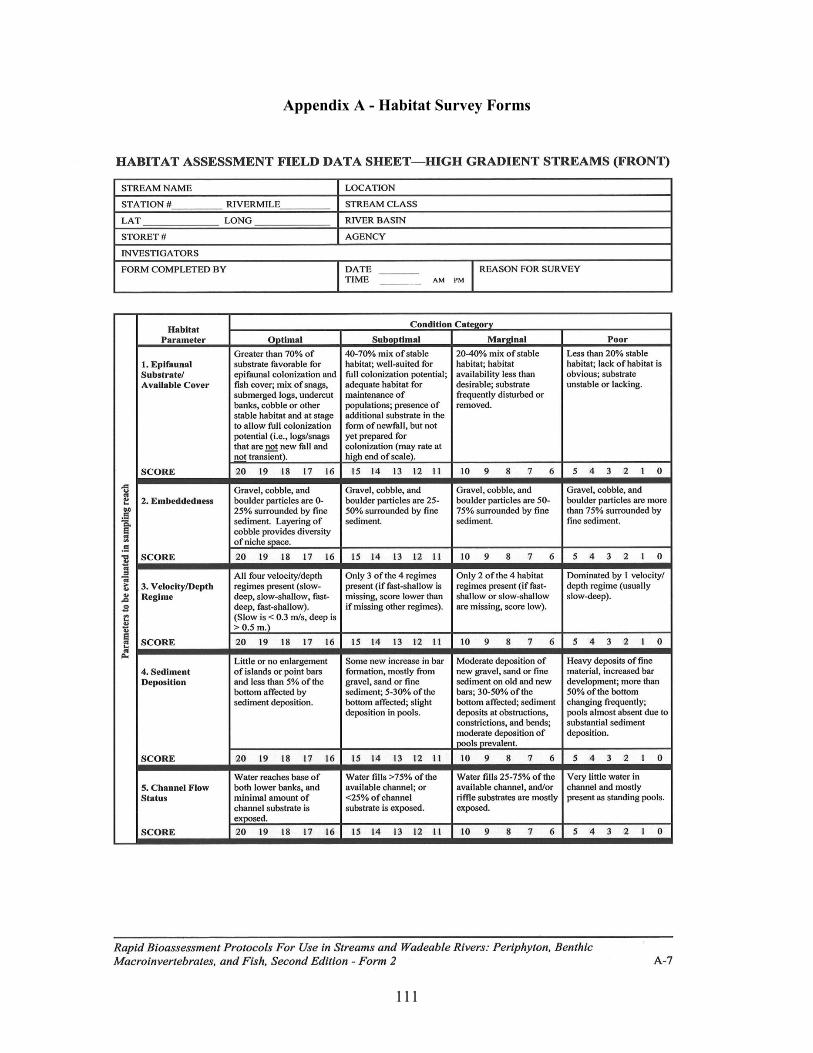
111
Appendix A - Habitat Survey Forms
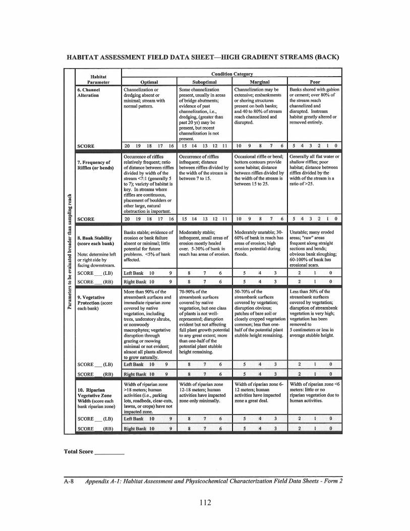
112
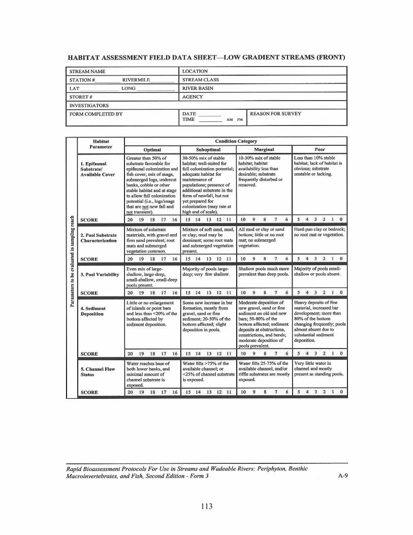
113
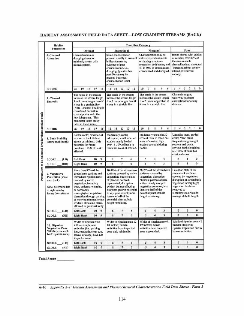
114
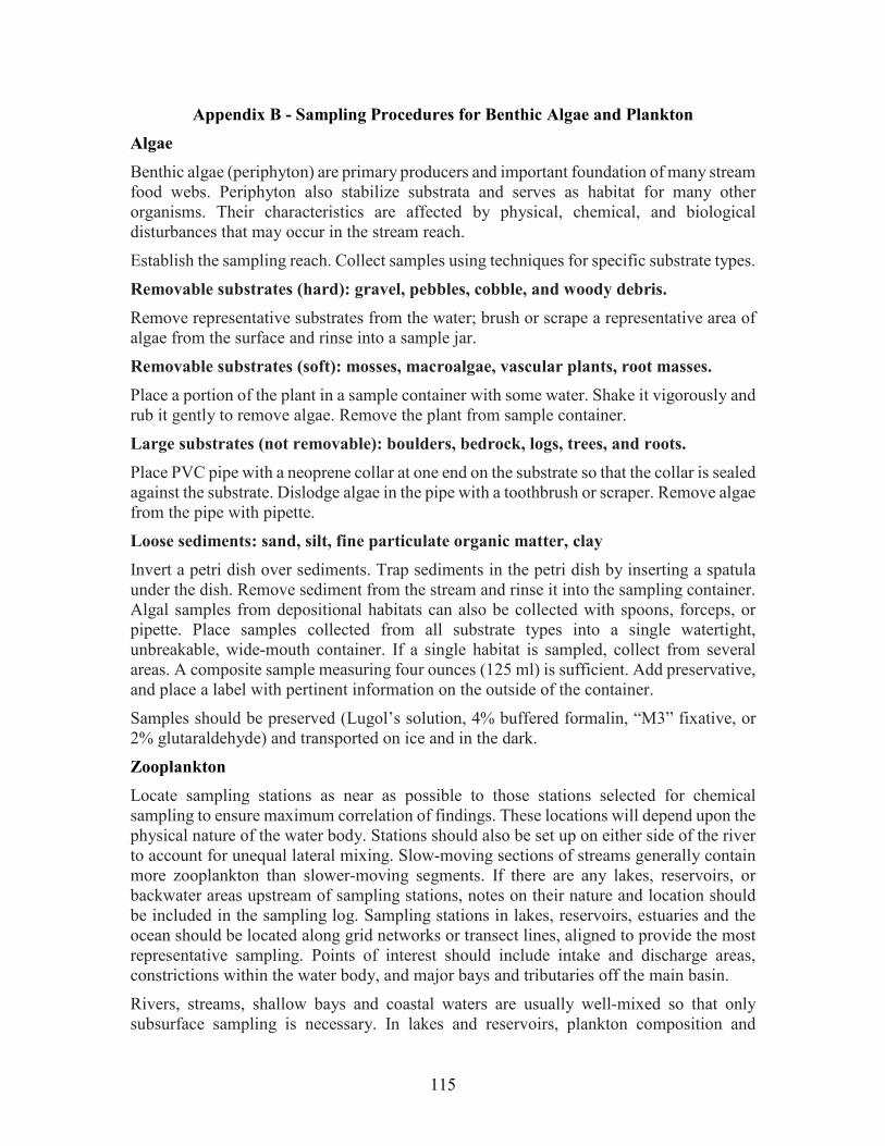
115
Appendix B - Sampling Procedures for Benthic Algae and Plankton Algae Benthic algae (periphyton) are primary producers and important foundation of many stream food webs. Periphyton also stabilize substrata and serves as habitat for many other organisms. Their characteristics are affected by physical, chemical, and biological disturbances that may occur in the stream reach.
Establish the sampling reach. Collect samples using techniques for specific substrate types.
Removable substrates (hard): gravel, pebbles, cobble, and woody debris. Remove representative substrates from the water; brush or scrape a representative area of algae from the surface and rinse into a sample jar.
Removable substrates (soft): mosses, macroalgae, vascular plants, root masses. Place a portion of the plant in a sample container with some water. Shake it vigorously and rub it gently to remove algae. Remove the plant from sample container.
Large substrates (not removable): boulders, bedrock, logs, trees, and roots. Place PVC pipe with a neoprene collar at one end on the substrate so that the collar is sealed against the substrate. Dislodge algae in the pipe with a toothbrush or scraper. Remove algae from the pipe with pipette.
Loose sediments: sand, silt, fine particulate organic matter, clay Invert a petri dish over sediments. Trap sediments in the petri dish by inserting a spatula under the dish. Remove sediment from the stream and rinse it into the sampling container. Algal samples from depositional habitats can also be collected with spoons, forceps, or pipette. Place samples collected from all substrate types into a single watertight, unbreakable, wide-mouth container. If a single habitat is sampled, collect from several areas. A composite sample measuring four ounces (125 ml) is sufficient. Add preservative, and place a label with pertinent information on the outside of the container.
Samples should be preserved (Lugol’s solution, 4% buffered formalin, “M3” fixative, or 2% glutaraldehyde) and transported on ice and in the dark.
Zooplankton Locate sampling stations as near as possible to those stations selected for chemical sampling to ensure maximum correlation of findings. These locations will depend upon the physical nature of the water body. Stations should also be set up on either side of the river to account for unequal lateral mixing. Slow-moving sections of streams generally contain more zooplankton than slower-moving segments. If there are any lakes, reservoirs, or backwater areas upstream of sampling stations, notes on their nature and location should be included in the sampling log. Sampling stations in lakes, reservoirs, estuaries and the ocean should be located along grid networks or transect lines, aligned to provide the most representative sampling. Points of interest should include intake and discharge areas, constrictions within the water body, and major bays and tributaries off the main basin.
Rivers, streams, shallow bays and coastal waters are usually well-mixed so that only subsurface sampling is necessary. In lakes and reservoirs, plankton composition and
116
density may vary with depth; therefore, sampling should be done at several depths determined by the depth of the thermocline; the euphotic zone, if applicable; and overall depth at the station. In shallow areas (one to two meters) subsurface samples (to a depth of one meter) are usually sufficient. In lentic environments, sample at one-meter intervals from the surface to the lake bottom because these organisms are not confined to the euphotic zone.
Zooplankton analysis requires at least six liters in moderately and highly productive waters. Sample size, preservation and storage are dependent upon certain variables. Refer to the NJDEP Field Sampling Manual for details. Generally, freshwater samples for species composition analysis should be preserved with a solution of neutralized formalin (5 ml neutralized buffer with formalin/100 ml of sample). All preserved samples should be stored in the dark immediately.
When collecting live samples, leave at least a four-cm air space in the bottle and chill to 4º C (e.g., in a cooler with ice) during transit storage. For delicate flagellated species, do not refrigerate sample bottles. Maintain in situ temperature by storing them out of direct sunlight, in an ice chest, with some of the ambient water. Surface samples in streams, rivers, shallow estuaries and coastal water can be collected simply by inverting the sample bottle, immersing it up to one meter below the water surface and slowly filling it as it is removed from the water. A Kemmerer sampler may also be used by holding it in a horizontal position and closing it manually. Samples collected for chlorophyll analysis should not be fixed or preserved. Chlorophyll samples should be preserved by chilling to 4°C. If species composition analysis is necessary, then samples should be collected in a separate sample bottle, or fixed or preserved by laboratory staff after the aliquot for chlorophyll analysis is removed from the sample container.
When deeper samples are needed, use of a Kemmerer, water bottle, Van Dorn or Juday samplers is standard. All of these sampling devices basically consist of a metal or plastic hollow cylinder with remotely activated stoppers at both ends. The sampler is lowered to a desired depth with a graduated line. Once at the desired depth, a heavy brass slug or “messenger” attached to the line is released. It slides down the line, and strikes the release mechanism on the sampler which pulls the stoppers tight against the open ends of the cylinder, trapping the sample of water inside. The sampler is then withdrawn and the water emptied into the sample container via a small spigot or tube in one of the stoppers. Use only nonmetallic samplers when metal analysis, algal assays, or primary productivity measurements will be performed on the sample. Sample bottle labels should identify the body of water sampled and list the date of collection, collectors name, preservative if present, and the type of biological analysis desired (determination of dominant or bloom species, total cell count, etc.). It is important that labels clearly identify live plankton samples as being unpreserved.
117
Appendix C - Surface Water Toxicity Testing Freshwater Test Species The most commonly used species for freshwater (salinity of 3.5 ppt or less) surface water toxicity studies in New Jersey are the fathead minnow (Pimephales promelas) and the water flea (Ceriodaphnia dubia). Rainbow trout (Oncorhynchus mykiss) and brook trout (Salvelinus fontinalis) are listed in the USEPA guidance, and brown trout (Salmo trutta) and bluegill (Lepomis macrochirus) are listed in the NJDEP guidance, but these fish species are not commonly used in New Jersey. Two other daphnid species (Daphnia pulex and Daphnia magna) are also listed in both the USEPA and NJDEP guidance, but are not commonly used in New Jersey.
Saltwater Test Species The most commonly used species for saltwater (salinity greater than 3.5 ppt) surface water toxicity studies in New Jersey are the sheepshead minnow (Cyprinodon variegatus) and the opossum shrimp (Americamysis bahia). Three other fish species ― inland silversides (Menidia beryllina), Atlantic silverside (M. menidia) and the tidewater silverside (M. peninsulae) ― are also listed in both the USEPA and NJDEP guidance but are not commonly used in New Jersey. The USEPA guidance lists a sea urchin (Arbacia punctulata) and a macroalga (Champia parvula), and the NJDEP guidance lists grass shrimp (Paleomonetes pugio), but these last three are rarely, if ever, used in New Jersey.
Toxicity Test Types There are three basic types of aqueous toxicity tests:
(1) static, nonrenewal tests in which the test solution is not changed throughout the test. These tests have the advantages of being simple, with minimal physical disturbance of the test organisms, and the disadvantage that toxicants may volatilize or degrade during testing;
(2) static-renewal tests in which the test organisms are exposed to fresh test solution periodically (e.g., every 24 hours). These have the advantage of being able to address the volatilization/degradation issue but are more labor-intensive and cause more physical disturbance to the test organisms; and
(3) flow-through tests in which there is a continual or semi-continual flow of fresh test solution through the test chambers for the duration of the test. These tests have the advantage of exposing organisms in a more stream-like manner, but these tests are significantly more labor-intensive and are also more expensive than the other two test types.
Toxicity Test Duration - Acute or Chronic Toxicity is generally assessed in the laboratory using acute or chronic studies. Acute studies are of short duration, usually one to four days, and are designed to determine whether the surface water sample in question will kill the exposed organisms. Chronic studies are longer, usually seven days or more (some exceeding 90 days), and are designed to determine sublethal effects on growth and reproduction. While observed lethality is a direct indication that the sample in question is toxic, sublethal effects are important for the assessment of long-term population health and are generally the endpoint of concern in an ecological risk assessment (ERA).
118
If no historical aquatic toxicity information is available, investigators can perform 24-hour to 96-hour acute toxicity studies to determine whether the samples are acutely toxic. If no acute toxicity is observed, investigators can initiate short-term chronic toxicity studies. Acute toxicity studies are quicker and cheaper than chronic studies. However, because aqueous samples can be diluted, it is often easier to go straight to the short-term chronic toxicity test, including a series of dilutions (sample mixed with clean laboratory water). For ERAs, chronic studies are often more appropriate because of the long-term exposure of the receptors to the contaminant of potential ecological concern (COPECs) (assessment of maintenance and reproduction of a healthy population).
Toxicity Test Design Aquatic toxicity studies are conducted by exposing a predetermined number of organisms (e.g., four replicates of ten organisms) to an undiluted sample or to a series of concentrations of a surface water or wastewater sample. Aquatic organisms are placed in appropriate test chambers (e.g., beakers, flasks, test tubes) containing the samples, and in test chambers containing clean laboratory water to serve as an experimental control. Investigators make direct observations of the exposed test organisms at regular intervals for the duration of the test to determine responses such as mortality, reduction in growth, or reduced reproduction.
Surface water and wastewater samples can be tested undiluted at 100 percent strength; however, if toxicity is observed, such a test does not indicate how toxic the sample is. Both USEPA and NJDEP recommend using five serial dilutions of the sample water (e.g., 100%, 50%, 25%, 12.5% and 6.25%) mixed with clean laboratory water. The clean laboratory water is also used as a negative control to assess the health of the test organisms (if toxic effects are noted in laboratory water, the batch of test organisms is considered suspect, and the test may have to be re-run using a different batch of organisms). A second “reference” control can also be included in the study, using surface water from outside the influence of the site (e.g., upstream).
To perform statistical analyses to determine whether significant differences exist between the laboratory controls or reference area samples, toxicity studies should be set up with multiple replicates. As a general rule, more replicates mean greater statistical power and more confidence in the final results. Acute toxicity studies are typically performed with two replicates of ten organisms for each test concentration, which is sufficient for calculation of lethal concentrations.
Short-term chronic toxicity studies should be performed with four or more replicates of ten organisms per exposure concentration for fish and mysid shrimp, and with ten replicates of a single organism per exposure concentration for Ceriodaphnia. Replication ensures sufficient statistical power for the more sensitive sublethal endpoints (e.g., growth and reproduction).
Toxicity Test Endpoints For acute toxicity studies, the typical endpoint is lethality, which is generally expressed as the LC50 (the concentration of test water that kills half of the exposed organisms). Statistical calculation methods are discussed at length in the USEPA guidance manual.
119
Short-term chronic studies, endpoints include lethality, growth, or reproduction. Tests may include the following:
• The seven-day fathead minnow larval survival and growth assay (USEPA Method 1000), and the seven-day sheepshead minnow larval survival and growth assay (USEPA Method 1004) assess survival at test termination as a percentage of the number of fish exposed at test initiation. Growth is assessed as the dry weight of the surviving fish.
• The seven-day daphnid survival and reproduction assay (USEPA Method 1002) also assesses survival at test termination. Reproduction is assessed by comparing the total number of progeny produced by each female in each test exposure at test termination. Ceriodaphnia are parthenogenic (meaning the female does not need a male to fertilize her eggs) and will generally produce three broods of progeny in seven days. Ten replicates, each with a single Ceriodaphnia, are monitored daily for the number of progeny released.
• The seven-day mysid shrimp survival, growth, and fecundity assay (USEPA Method 1007) also assesses survival at test termination. Fecundity is assessed by microscopic evaluation of all surviving organisms to determine their sex and the percentage of surviving females that are carrying eggs. After fecundity counts, growth is assessed as the dry weight of the surviving shrimp.
Data Evaluation
The seven-day short-term chronic endpoints include the LC50, the no observed effect concentration (NOEC) and the lowest observed effect concentration (LOEC). The NOEC is the highest test concentration at which there was no statistically significant reduction in survival, growth, or reproduction or fecundity as compared to the laboratory control or reference area sample. The LOEC is the lowest test concentration at which a significant reduction was observed. The inhibitory concentration (IC) can also be calculated for any percentage of concern. For example, the IC25 is the test concentration that yielded an inhibitory effect on 25 percent of the exposed organisms.
All statistical analyses are to be performed as specified in the USEPA guidance manuals. Statistical programs developed specifically for aquatic toxicity studies are commercially available. Data from site samples should be compared to the laboratory controls to determine whether observed toxic effects are statistically significant. In addition to the laboratory control, an appropriately selected field reference area sample may yield results that are more representative of actual field conditions. A surface water sample from upstream of a site is an appropriate reference area for a surface water sample from downstream of a site. If the upstream reference area sample shows toxic effects, it is possible that at least a portion of any toxic effect observed from the downstream sample is not related to the site.
Quality Assurance All toxicity studies should meet the minimum test acceptability criteria for control organism survival, growth, reproduction or fecundity set forth in the appropriate guidance documents. Additionally, Standard Reference Toxicant (SRT) tests should be performed by the laboratory at regular intervals (at least monthly for surface water species). It is preferable that the SRT be initiated on the same day, by the same technicians, with the

120
same batch of organisms used for the test samples (so the SRT is directly related to the study). The lab should have a reference toxicant control chart for each species and age group they regularly use in testing. The object of the SRT is to assess the organism health, the lab procedure, and the technician's handling.
121
Appendix D - Sediment Toxicity Testing Freshwater Test Species Two benthic invertebrate species are usually tested simultaneously for freshwater (salinity of 3.5 ppt or less) sediment toxicity studies in New Jersey. They are the amphipod (Hyalella azteca) and the midge (Chironomus dilutus). Other potentially appropriate species mentioned in the USEPA and ASTM guidance include the amphipod (Diporeia spp.), the midge (Chironomus riparius) the mayfly (Hexagenia spp.) and the oligochaete worms Lumbriculus variegatus and Tubifex tubifex.
H. azteca and C. dilutus are usually tested simultaneously to incorporate their varying sensitivities and their different exposure pathways. H. azteca is epibenthic (lives and feeds on top of the sediment, hidden by leaves and organic detritus), while C. dilutus burrows directly into the sediment. This distinction is important in situ, but in laboratory studies, no leaves or cover objects are added to the test chambers, so both species burrow directly into the sediment. Testing is performed in accordance with USEPA (2000a) and ASTM (2005a) guidance.
Saltwater Test Species The most commonly used benthic invertebrates for estuarine and marine sediment toxicity testing in New Jersey are the amphipods, Leptocheirus plumulosus and Ampelisca abdita, and the polychaete worms Neanthes arenaceodentata and Neanthes virens. Other amphipod species included in the ASTM methods are Eohaustorius estuarius and Rhepoxynius abronius, Pacific species that are not applicable for use in New Jersey.
Marine sediment toxicity testing is usually performed with a single amphipod species. L. plumulosus is more appropriate for lower salinity (5 to 20 ppt), estuarine sediment samples, and A. abdita is more appropriate for higher salinity (20 to 35 ppt), marine sediment samples.
Because of their relatively large size and available tissue mass, the polychaete worms N. arenaceodentata and N. virens are used for bioaccumulation studies in which the worms are exposed to a test sediment for a specified time (e.g., 28 days) and then the tissue is submitted for analysis of contaminants of concern.
Toxicity Test Types There are three basic types of sediment toxicity tests:
(1) static, nonrenewal tests, in which the overlying water is not changed throughout the test. These have the advantages of being simple, with minimal physical disturbance of the sediment or test organisms, and the disadvantage that the ammonia and oxygen demand from the sediment may confound the results;
(2) static-renewal tests in which the overlying water is exchanged periodically (e.g., every 12 hours). These have the advantage of being able to address the ammonia and dissolved oxygen issues but are more labor intensive and cause more physical disturbance to the sediment and test organisms; and
(3) flow-through tests in which there is a continual or semi-continual flow of fresh overlying water through the test chambers for the duration of the test. These have the advantage of exposing organisms in a more stream-like manner, but they are
122
significantly more labor intensive and are also more expensive than the other two test types.
Toxicity Test Duration - Acute or Chronic Sediment toxicity is generally assessed in the laboratory using acute or chronic studies. Acute sediment studies take ten days (though screening assays may be shorter), and are designed to determine whether the sediment sample in question will kill the exposed organisms or impact their growth. Chronic studies are longer, usually 20 days or more (some exceeding 50 days), and are designed to determine sublethal effects on growth, emergence and reproduction. While observed lethality is a direct indication that the sample in question is toxic, sublethal effects can be important for the assessment of long-term population health. In ecological risk assessments, chronic toxicity tests are generally considered to be the preferred alternative. The NJDEP and USEPA Region 2 BTAG have routinely recommended the use of ASTM E1706 - 05(2010) Standard Test Method for Measuring the Toxicity of Sediment-Associated Contaminants with Freshwater Invertebrates. The previous version of this standard (Test Method E1706-95b) described 10-day toxicity tests with the amphipod Hyalella azteca and midge Chironomus. This version of the standard now outlines approaches for evaluating sublethal endpoints in longer-term sediment exposures with these two species (Annex A6 and Annex A7).
However, in highly urbanized settings where there are numerous sources effecting a site, the longer-term sublethal studies are not always appropriate for environmental sediment samples because the short-term toxicity tests are adequate to measure potential impacts associated with the site. Sensitive sublethal tests are good for testing chemicals and wastewater solutions that can be diluted to different concentrations (e.g., 100%, 50%, 25%, 12.5% and 6.25%) at which a dose response becomes apparent. If a response unrelated to dose is observed (e.g., effect at 25%, but not at 100%), the test is suspect. When testing sediment samples, they are not diluted and are tested as 100 percent versus a laboratory control or reference area sample. If there is a sublethal effect, investigators may not be able to tell whether it is related to the sample or to the inherent variability of the biological system being tested.
Variability is expected even in the laboratory's Standard Reference Toxicant (SRT) studies. Labs perform regular SRT tests to assess the health of each batch of test organisms and the procedures used by the technicians setting up the tests. The SRT studies are typically short-term (96 hours or shorter), water-only tests that use a common reagent-grade salt (e.g., KCl). The USEPA (2000a) states that even though the final SRT result is allowed to fall within two standard deviations of the laboratory's historical mean, the laboratory is expected to have up to 10 percent of SRT tests fall outside of that range. It is not until the lab has more than 10 percent SRT failures that a problem is noted. Because USEPA expects so much variability in a short-term test with lab water and reagent salts, it is within reason to expect that long-term, sublethal effects from complex mixtures like site sediment will yield substantially more variability.
123
Toxicity Test Design Sediment toxicity studies are conducted by exposing a predetermined number of organisms (e.g., eight replicates of ten organisms) to a sediment sample. Benthic organisms are placed in beakers containing a layer of the sediment sample covered with clean laboratory water, and in test chambers containing clean laboratory sediment to serve as an experimental control. Investigators make direct observations of the exposed test setup at regular intervals for the duration of the test to determine responses such as erratic behavior and visible mortality. However, sediment organisms quickly bury themselves in the test sediment and are not seen again until test termination when they are removed for final enumeration.
A second “reference” control should also be included in each study, using sediment from outside the influence of the site (e.g., upstream). Use of an appropriate reference area sediment is more representative of the actual background area stream conditions. While a site sediment may show a significant effect as compared to the laboratory control, it may not show a significant effect when compared to the reference area.
To perform statistical analyses to determine whether significant differences exist between the site-related samples and laboratory controls or reference area samples, toxicity studies should be set up with multiple replicates. As a general rule, more replicates mean greater statistical power and more confidence in the final results. Acute sediment studies are typically performed with eight replicates of ten organisms for each test sample, which ensures sufficient statistical power for the more sensitive sublethal growth endpoint.
Toxicity Test Endpoints For acute sediment toxicity studies, the endpoints include survival and growth. Survival is assessed as a percentage of the number of organisms exposed at test initiation. Growth of amphipods, both freshwater and saltwater, is assessed as the dry weight of the surviving organisms.
Growth of midges is assessed as the ash-free dry weight (AFDW) of the surviving organisms. Sediment grain size influences the amount of sediment that C. dilutus larvae ingest, and as a result, larvae exposed to finer-grained sediment will have more sediment in their guts. Because most sediment sites have varying grain size distributions, significant bias can be added to the C. dilutus growth results. By measuring the dry weight of the surviving organisms at test termination, then ashing them to burn off any organic material, the weight of the sediment grains can be subtracted from the total dry weight to yield AFDW, which is the more appropriate endpoint.
Data Evaluation
All statistical analyses are to be performed as specified in the USEPA and ASTM guidance documents. Data from site samples should be compared to the laboratory controls to determine whether observed toxic effects are statistically significant. In addition to the laboratory control, an appropriately selected field reference area sediment may yield results that are more representative of actual background area field conditions. If the upstream reference area sample shows toxic effects, it is possible that at least a portion of any toxic effect observed from the downstream sample is not related to the site.
124
Quality Assurance All toxicity studies should meet the minimum test acceptability criteria for control organism survival, growth, reproduction or fecundity set forth in the appropriate guidance documents. Additionally, SRT tests should be performed by the laboratory at regular intervals (at least monthly for surface water species). It is preferable that the SRT be initiated on the same day, by the same technicians, with the same batch of organisms used for the test samples (so the SRT is directly related to the study). The lab should have a reference toxicant control chart for each species and age group they regularly use in testing. The object of the SRT is to assess the organism health, the lab procedure and the technician's handling.
125
Appendix E - Sediment Pore Water and Elutriate Toxicity Testing Freshwater Test Species The most commonly used species for freshwater (salinity of 3.5 ppt or less) surface water toxicity studies in New Jersey are the fathead minnow (Pimephales promelas) and the water flea (Ceriodaphnia dubia). These species would also be appropriate for testing of sediment pore water and elutriate samples.
Salt Water Test Species The most commonly used species for saltwater (salinity greater than 3.5 ppt) surface water toxicity studies in New Jersey are the sheepshead minnow (Cyprinodon variegatus) and the opossum shrimp (Americamysis bahia). These species would also be appropriate for testing of sediment pore water and elutriate samples.
Toxicity Test Types There are three basic types of aqueous toxicity tests:
(1) static, nonrenewal tests, in which the test solution is not changed throughout the test. These have the advantages of being simple, with minimal physical disturbance of the test organisms, and the disadvantage that toxicants may volatilize or degrade during testing;
(2) static-renewal tests in which the test organisms are exposed to fresh test solution periodically (e.g., every 24 hours). These have the advantage of being able to address the volatilization and degradation issues, but are more labor intensive and cause more physical disturbance to the test organisms; and
(3) flow-through tests, in which there is a continual or semi-continual flow of fresh test solution through the test chambers for the duration of the test. These have the advantage of exposing organisms in a more stream-like manner, but they are significantly more labor intensive and are also more expensive than the other two test types.
Flow-through assays are difficult to perform with pore water and elutriate samples because of the volumes of sample required. Therefore, the static-renewal and the static-nonrenewal are the most commonly performed test types.
Toxicity Test Duration - Acute or Chronic Toxicity is generally assessed in the laboratory using acute or chronic studies. Acute studies are of short duration, usually one to four days, and are designed to determine whether the sediment pore water or elutriate sample in question will kill the exposed organisms. Chronic studies usually take seven days and are designed to determine sublethal effects on growth and reproduction. While observed lethality is a direct indication that the sample in question is toxic, sublethal effects are important for assessing long-term population health.
If no historical aquatic toxicity information is available, investigators can perform 24-hour to 96-hour acute toxicity studies to determine whether the samples are acutely toxic. If no acute toxicity is observed, investigators can initiate short-term chronic toxicity studies. Acute toxicity studies are quicker and cheaper than chronic studies. However, because aqueous samples can be diluted, it is often easier to go straight to the short-term chronic
126
toxicity test, including a series of dilutions (pore water or elutriate sample mixed with clean laboratory water).
Toxicity Test Design Aquatic toxicity studies are conducted by exposing a predetermined number of organisms (e.g., four replicates of ten organisms) to an undiluted sample or to a series of concentrations of a pore water or elutriate sample. Aquatic organisms are placed in appropriate test chambers (e.g., beakers, flasks, test tubes) containing the samples and in test chambers containing clean laboratory water to serve as an experimental control. Investigators make direct observations of the exposed test organisms at regular intervals for the duration of the test to determine responses such as mortality, reduction in growth or reduced reproduction.
Pore water and elutriate samples can be tested undiluted, at 100 percent strength, but if toxicity is observed, such a test does not indicate how toxic the sample is. For surface water and wastewater assays, both the USEPA and NJDEP recommend using five serial dilutions of the sample water (e.g., 100%, 50%, 25%, 12.5% and 6.25%) mixed with clean laboratory water. The clean laboratory water is also used as a negative control to assess the health of the test organisms (if toxic effects are noted in laboratory water, the batch of test organisms is considered suspect, and the test may have to be re-run using a different batch of organisms). A second “reference” control can also be included in the study, using pore water or elutriate derived from sediment samples collected outside the influence of the site (e.g., upstream).
To perform statistical analyses to determine whether significant differences exist between the laboratory controls or reference area samples, toxicity studies should be set up with multiple replicates. As a general rule, more replicates mean greater statistical power and more confidence in the final results. Acute toxicity studies are typically performed with two replicates of ten organisms for each test concentration, which is sufficient for calculation of lethal concentrations.
Short-term chronic toxicity studies should be performed with four or more replicates of ten organisms per exposure concentration for fish and mysid shrimp, and with ten replicates of a single organism per exposure concentration for Ceriodaphnia. Replication ensures sufficient statistical power for the more sensitive sublethal endpoints (e.g., growth and reproduction).
Toxicity Test Endpoints For acute toxicity studies, the typical endpoint is lethality. Lethality is generally expressed as the LC50 (the concentration of test water that kills half of the exposed organisms). Statistical calculation methods are discussed at length in the USEPA guidance manual.
For short-term chronic studies, endpoints include lethality, growth or reproduction endpoints. The seven-day fathead minnow larval survival and growth assay (USEPA Method 1000) and the seven-day sheepshead minnow larval survival and growth assay (USEPA Method 1004) assess survival at test termination as a percentage of the number of fish exposed at test initiation. Growth is assessed as the dry weight of the surviving fish.
The seven-day daphnid survival and reproduction assay (USEPA Method 1002) also assesses survival at test termination. Reproduction is assessed by comparing the total
127
number of progeny produced by each female in each test exposure at test termination. Ceriodaphnia are parthenogenic (meaning the female does not need a male to fertilize her eggs), and will generally produce three broods of progeny in seven days. Ten replicates, each with a single Ceriodaphnia are monitored daily for the number of progeny released.
The seven-day mysid shrimp survival, growth and fecundity assay (USEPA Method 1007) also assesses survival at test termination. Fecundity is assessed by microscopic evaluation of all surviving organisms to determine their sex and the percentage of surviving females carrying eggs. After fecundity counts, growth is assessed as the dry weight of the surviving shrimp.
Data Evaluation
The seven-day short-term chronic endpoints include the LC50, the NOEC and the LOEC. The NOEC is the highest test concentration at which there was no statistically significant reduction in survival, growth, reproduction or fecundity as compared to the laboratory control or reference area sample. The LOEC is the lowest test concentration at which a significant reduction was observed. The IC can also be calculated for any percentage of concern. For example, the IC25 is the test concentration that yielded an inhibiting effect on 25 percent of the exposed organisms.
All statistical analyses are to be performed as specified in the USEPA guidance manuals. Statistical programs developed specifically for aquatic toxicity studies are commercially available. Data from site samples should be compared to the laboratory controls to determine whether observed toxic effects are statistically significant. In addition to the laboratory control, an appropriately selected field reference area sample may yield results that are more representative of actual field conditions. A pore water or elutriate sample derived from sediment collected upstream of a site is an appropriate reference area for a pore water or elutriate sample derived from site sediment. If the upstream reference area sample shows toxic effects, it is possible that at least a portion of any toxic effects observed from the downstream sample is not related to the site.
Quality Assurance All toxicity studies should meet the minimum test acceptability criteria for control organism survival, growth, reproduction or fecundity set forth in the appropriate guidance documents. Additionally, standard reference toxicant (SRT) tests should be performed by the laboratory at regular intervals (at least monthly for surface water species). It is preferable that the SRT be initiated on the same day, by the same technicians, with the same batch of organisms used for the test samples (so the SRT is directly related to the study). The lab should have a reference toxicant control chart for each species and age group they regularly use in testing. The object of the SRT is to assess the organism health, the lab procedure and the technician's handling.
128
Appendix F – Sediment Pore Water Sampling Techniques The following briefly describes some of the more recent tools and methods used for the collection of sediment pore water samples. A detailed discussion of each method is beyond the scope of this guidance. Rather, this section is intended to simply introduce these methods and provide references for their use and interpretation of data generated. Ultimately, the use of these methods should result in a more accurate measure of site-specific contaminant bioavailability or toxicity to sediment dwelling organisms. Diffusion Samplers Diffusion-based samplers consist of a semipermeable membrane or dialysis tube filled with distilled water, purified fish oil (triolein) or a gel, which rely on a solute gradient to establish equilibrium between the pore water and the sampler. Diffusion samplers are often used in situ for measuring metals, phosphates, and sulfides. Some of the more common samplers for in situ diffusion include the following:
• Peepers: A sampling device, also referred to as a dialysis cell, which consists of a rigid structure that can hold volumes of distilled or deionized water separated from the environment by a porous membrane. Holes within the rigid structure allow pore water and associated contaminants to pass through the membrane, allowing the cell to passively equilibrate with the surrounding pore water. These samplers are capable of monitoring most compounds (inorganic and organic) present in dissolved phases (ITRC, 2005).
• Semi-Permeable Membrane Devices (SPMD): SPMDs are fat- or lipid-filled membranes that attempt to mimic uptake into benthos or fish in terms of HOC (hydrophobic organic chemical) absorption to lipids in aquatic organisms (Zimmerman, et al., 2000). SPMDs consist of a high molecular weight lipid (typically triolein) that is placed into a polyethylene membrane tube. The device may be placed in a perforated stainless steel deployment device to provide protection when placed in sediment (USEPA, n.d.).
• Diffusive gradient in thin films (DGT): DGTs are another type of diffusion sampler, and refers to two similar tools for collecting metals from sediment pore water (Davison et al., 2000). DGTs differ from other diffusive samplers in that they are typically casings filled with gels that are specific to the target compound (e.g., a Chelex or acrylamide gel for metals, ferrous-oxide gel for phosphorus). The unique advantage of DGTs over other diffusive samplers is that after retrieval, the gel can be cut into segments for multiple analyses.
Equilibrium Samplers Equilibrium samplers are used to measure the pore water concentrations of freely dissolved hydrophobic organic compounds (e.g., PCBs, PAHs). These types of samplers can be deployed in situ (e.g., directly into the sediment) where they accumulate contaminants from the pore water, while others are used to extract small quantities of contaminants from extracted pore water.
• Solid Phase Microextraction Devices (SPME): This technique, used to establish PAH pore water concentrations, involves using thin silica fibers coated with an organic polymer. The fibers can be exposed to sediment pore water in situ or in a laboratory setting. The freely dissolved hydrophobic organic contamination is sorbed onto the
129
SMPE fiber, which is then injected into a GS/MS for analysis. The direct pore water results are then evaluated using USEPA’s hydrocarbon narcosis model (USEPA, 2003). It has been documented that the ability of the SPME method to predict toxicity correlate well with toxicity observed with standard sediment toxicity tests. This technique was more reliable at predicting PAH impacts than were those found through the use of bulk PAH concentrations and Equilibrium Partitioning (EqP) to estimate pore water concentrations (Moles et al., 2006; Hawthorne et al., 2007). The method recently became standardized (USEPA SW-846 Method 8272/ASTM provisional standard D7363-07) and incorporated into USEPA’s document titled Evaluating Ecological Risk to Invertebrate Receptors from PAHs in Sediments at Hazardous Waste Sites (2009d). http://cfpub.epa.gov/ncea/cfm/recordisplay.cfm?deid=214715
• Polyethylene (PE) and polyoxymethylene (POM) samplers: These samplers are similar to SPMEs in their ability to sorb organic compounds from sediments. A principal advantage of using these samplers is their ability to come into equilibrium faster than SPMEs. Recent work has shown that uptake of PAH and PCBs by PE and POM samplers correlate with benthic organism uptake (Tomasaewski and Luthy, 2008).
Centrifugation Centrifugation is another method used for the collection of pore water samples. This method involves placing bulk sediments in a large-capacity centrifuge (e.g., a bucket-style centrifuge with one-liter capacity per sample) and centrifuging them at low speed (e.g., 7,400 x gravitational force) for 15 to 30 minutes (ASTM, 2000; Environment Canada, 1994). In some cases, subsequent high-speed centrifugation (e.g., 10,000 x gravitational force) may be necessary or desirable, particularly if the selected test species have low tolerance to suspended particles. Centrifugation requires the collection of a large volume of sediment to extract a sufficient amount of pore water suitable for analysis, often contributing to elevated method detection limits (MDLs).
Additional Pore Water Sampling Devices One additional pore water sampling device that is unique in that it measures three parameters is the US Navy’s Trident probe. The Trident probe is a flexible, multi-sensor, water-sampling probe for screening and mapping groundwater plumes at the surface water interface. The probe has the ability to measure conductivity, temperature, and pore water, and is well-suited for spatially identifying where groundwater is discharging to surface water. Once the groundwater and surface water discharge is located, pore water samples can be collected to chemically characterize the contamination. https://www.clu-in.org/programs/21m2/navytools/gsw/
130
Appendix G – Invertebrate Sampling Methods Methods for sampling invertebrates include the use of artificial substrates, Surber samplers, grab samplers and Rapid Bioassessment techniques. These are described below (modified text taken directly from the Field Sampling Procedures Manual (NJDEP, 2005) and Rapid Bioassessment Protocols for Use in Streams and Wadeable Rivers (USEPA, 1999b).
All benthic macroinvertebrates are preserved in 5 percent formalin (5 ml formalin/100 ml of water from which the organism was taken), with 95 percent ethanol, or isopropyl alcohol. A Mason jar, or any glass or plastic wide mouth container can be used for benthic macroinvertebrate samples.
Artificial Substrates: (Hester-Dendy) These multi-plate samplers consist of eight large tempered plates separated by seven small plates, exposing one square foot of surface area. A hole is bored through the center of each plate. Plates are placed alternatively on a galvanized eyebolt, threaded rod or nylon cord and secured. Samplers may have a brick attached to one end to anchor the sampler to the bottom for use in shallow streams, or they may be suspended from anchored floats in lakes and deep rivers. Used throughout, artificial substrates provide consistency of habitat to facilitate comparison among stations. Samplers are usually placed at equal intervals across a stream. However, species colonization is greatly affected by current velocity. When conducting a survey, care should be taken to place substrates at locations having similar flow characteristics. Three samplers are routinely placed at each sample site, although more samples may be necessary to satisfy particular statistical criteria. When using brick-anchored samplers, additional rocks are often necessary to secure the sampler upright. Care should be taken not to block the plates with the rocks and thus limit colonization. Sampling devices should be placed as inconspicuously as possible because they are prone to removal by the public. They should be secured with strong nylon line (not attached to the anchor line itself). In deeper waters, suspended samplers should be placed within the euphotic zone (i.e., shallower depths where light penetrates) usually less than 2 meters.
The samplers should be removed after a six-week colonization period. Gently remove the sampler from the water so as not to dislodge the organisms, and immediately place the sampler in a plastic tub or bucket. Anchors attached to the substrate should not be placed in the tub until any organisms on the anchor are removed and discarded. Add a small amount of water to the tub and wash the easily removable material from the plates. Then gently scrape the top and bottom of each plate into the tub, removing the plates as cleaned. Scalpel, spatula or soft toothbrushes are useful cleaning tools. Pour the sample slurry through a US Standard No. 30 sieve. Additional water may be used to completely clean the tub. Pass this through the sieve as previously described. Transfer the sample material from the sieve to the sample jars using forceps or a stream of water from a wash bottle. Fill each jar no more than half full. Work directly over the tub so that any spilled materials can be recovered. Finally, inspect the tub for any remaining organisms and transfer them to the sample jar(s). Water-resistant paper should be used for sample labels and all information written with a soft lead pencil. Include sample (log) number, water body, station, sample number, sample device, and other pertinent information.
131
Surber or Square-foot Bottom This sampler consists of a strong close-woven fabric (0.595-mm opening) approximately 69-cm (27 in.) long held open by a one-square-foot metal frame hinged at one side to another frame of equal size. The sampler is generally used in procuring samples in fast-flowing streams less than 1m deep. It can also be used in pools where the water depth is wadeable. Three replicate samples are usually obtained at each sampling station. Carefully place the sampler in position with the net opening facing upstream, using the current to hold the net open while standing downstream and to the side of the sampling area. By imbedding the separate two- or four-inch extensions of the horizontal frame, the sampled area will be more effectively isolated. When taking replicate samples, always work across or in an upstream direction. Dislodge the rocks, stones, and other bottom material within the frame to a depth of at least 2 inches and collect them in the net.
Remove the sampler and empty the contents into a plastic tub. Carefully inspect the larger rocks and stones removing any organisms clinging to them, and discard the stones when cleaned. Also, carefully inspect the net and remove any organisms remaining. After the larger materials have been inspected and removed, add a small amount of water to the tub and pour the slurry through an US Standard No. 30 sieve. This may have to be repeated several times to completely empty the tub.
Grab Samplers The Ponar, Peterson, and Ekman grab are the most commonly used grab samplers. The Ponar is similar to the Peterson except that it has side plates and a screened top to prevent sampling loss. The Ekman grab is useful in sampling silt and muck in water with little current. Extreme care should be employed when locking open the jaws of the samplers because premature tripping will squash or sever fingers or hands. Handling by the attached line is recommended with an open sampler. Carefully lower the grab to the bottom so as not to agitate the substrate prior to sampling. Slacken the rope to trip jaws (the Ekman grab employs a messenger, which is released by the operator) and retrieve the sampler. Place it in a plastic tub or large screened bin and carefully open the sampler jaws to release the sample. The sample should be discarded if sticks or stones have obstructed the jaws or if there is incomplete closure for any other reason. Inspect the larger debris for organisms and discard the debris when cleaned. Filter the sample through a #30 sieve to remove small particles.
Rapid Bioassessment Benthic rapid bioassessment procedures (RBPs) usually employ direct sampling of natural substrates, as do Surbers and grab samplers. Under certain conditions, however, such as in large rivers, the use of artificial substrates may be more appropriate for RBP analysis. The collection procedure should provide representative samples of the benthic macroinvertebrate fauna from comparable habitat (substrate) types at all stations in a particular survey. Either single or multiple habitat samples can be employed depending on which is more suitable for a particular survey. A riffle and run habitat with rock substrate will generally provide the most diverse community of major benthic macroinvertebrate groups. If the stream or river is not wadeable or has an unstable substrate, fixed structures (e.g., submerged boulders, logs, bridges, and pilings) can provide suitable habitat. D-
132
framed or rectangular framed 500 – 900 mm mesh “kick” nets can be employed as either single or multiple habitat samplers.
Single Habitat Sampling A 100-meter reach representative of the characteristics of the stream is chosen, and whenever possible, upstream of road or bridge crossing. A composite sample is taken from individual sampling spots in the riffles and runs in the stream reach. A minimum of 2m2 composited area is sampled. Sampling begins at the downstream end of the reach and proceeds upstream. Two to three kicks are sampled at various velocities in the reach. A kick is a stationary sampling accomplished by positioning the net on the bottom of the stream and disturbing one square meter upstream of the net. The substrate can be disturbed using the heel and toe of the boot or rubbed by hand for larger substrate particles. Several kicks will make up the composite sample. Empty the composite sample into a sieve or sieve bucket and mix to ensure a homogeneous composite.
Multi-habitat Sampling For sampling low-gradient streams or streams with variable habitats, a multi-habitat sampling approach is required. A 100-meter reach representative of the characteristics of the stream is chosen, and whenever possible, upstream of road or bridge crossing. Sampling begins at the downstream end of the reach and proceeds upstream. Habitats are sampled in their approximate proportion to their representation of surface area in the reach. In low-gradient streams, snags, vegetated banks, submerged macrophytes, and gravel and sand are habitats that support fauna. A total of 20 jabs or kicks should be sampled over the length of the reach. A kick is a stationary sampling accomplished by positioning the net on the bottom of the stream and disturbing one square meter upstream of the net. The substrate can be disturbed using the heel and toe of the boot or rubbed by hand for larger substrate particles. A jab consists of forcefully thrusting the net into a productive habitat for a linear distance of 0.5 meters. Then, sweep the area with a net to ensure that benthic macroinvertebrates that have disengaged from the substrate are collected. A minimum of two square meters of composited area is sampled. Empty the composite sample into a sieve or sieve bucket and mix to ensure a homogeneous composite.
133
Appendix H - Soil Toxicity Testing Soil Test Species The most commonly used invertebrate species for soil toxicity studies is the earthworm (Eisenia fetida). Other species mentioned in the ASTM guidance include the potworm (Enchytraeus albidus), and while use of potworms is appropriate, the earthworm can constitute up to 92 percent of the invertebrate biomass in soil (ASTM, 2004) and is, therefore, a more important receptor. Additionally, the earthworm has been more widely and commonly used by the USEPA. For these reasons, the earthworm is preferred.
Most plant toxicity testing guidance is geared toward agricultural crops, and test methods were developed for exposing crop plants to chemical products (e.g., pesticides). These methods can also be used for testing the effects of site soils on more appropriate site-related species. The noncrop plants most commonly used for soil toxicity testing include perennial ryegrass (Lolium perenne) and red clover (Trifolium pratense).
Toxicity Test Types There is basically a single type of soil toxicity test: static, nonrenewal. Worms or plant seeds are added to the soil at test initiation and removed from the soil at test termination. However, earthworm biomass loading is dependent on the soil’s total organic carbon (TOC) content, and toxicity tests have been performed where worms have been transferred to fresh site soil halfway through the study to avoid nutrition-related stress.
Toxicity Test Duration Soil toxicity is generally assessed in the laboratory using acute or chronic studies. Acute soil studies usually take 14 days (though earthworm screening assays may be shorter). Chronic studies are longer, usually 28 days or more (some exceeding 140 days), and are designed to determine sublethal effects on growth, emergence and reproduction. While observed lethality is a direct indication that the sample in question is toxic, sublethal effects are important for the assessment of long-term population health.
The longer term, sublethal studies are not always appropriate for environmental soil samples. They are very sensitive, and can yield false positives. Sensitive, sublethal tests are good for testing chemicals and wastewater solutions that can be diluted to different concentrations (e.g., 100%, 50%, 25%, 12.5% and 6.25%) at which a dose response becomes apparent. If a response not related to dose is observed (e.g., effect at 25%, but not at 100%), the test is suspect. When testing soil samples, they are not diluted and are tested as 100 percent versus a lab control reference area sample. If there is a sublethal effect, investigators may not be able to tell whether it is related to the sample or to the inherent variability of the biological system being tested.
Variability is expected even in the laboratory's standard reference toxicant (SRT) studies. Labs perform regular SRT tests to assess the health of each batch of test organisms and the procedures used by the technicians setting up the tests. The SRT studies are typically short-term (96 hours or shorter), water-only tests that use a common reagent-grade salt (e.g., KCl). The USEPA (2000a) states that even though the final SRT result is allowed to fall within two standard deviations of the laboratory's historical mean, the laboratory is expected to have up to 10 percent of SRT tests fall outside of that range. It is not until the lab has more than 10 percent SRT failures that a problem is noted. Because USEPA
134
expects that much variability in a short-term test with lab water and reagent salts, it is within reason to expect that long-term, sublethal effects from complex mixtures like site soil will yield substantially more variability.
Toxicity Test Design Soil toxicity studies are conducted by exposing a predetermined number of organisms (e.g., four replicates of ten organisms or seeds) to a soil sample. Organisms are placed in appropriate test chambers containing the soil sample, and in test chambers containing clean laboratory soil to serve as an experimental control. Investigators make direct observations of the exposed test setup at regular intervals for the duration of the test to determine responses such as erratic behavior and visible mortality. However, earthworms quickly bury themselves in the test soil and are not seen again until test termination when they are removed for final enumeration. Plants are not visible until after the seeds germinate and the plants begin to emerge after four to seven days.
A second “reference” control should also be included in the study, using soil from outside the influence of the site. Use of an appropriate reference area soil is more representative of the actual field conditions. While a site soil may show a significant effect as compared to the laboratory control, it may not show a significant effect when compared to the reference area.
The laboratory control soil should be an “artificial” soil, as described in the ASTM guidance (ASTM, 2004, Appendix A2). While both the plant and invertebrate toxicity methods allow for use of various artificial soil mixtures, potting soils or natural soils as laboratory controls, the objective of the study is not to compare site soils to “optimum” soil samples. Comparing the growth and reproduction of worms or plants grown in site soils to those grown in a laboratory control composed of a rich, organic potting soil will almost always show a significant decrease in site sample growth compared to the control, regardless of whether the site soil is toxic or not. For this reason, potting soil or any other rich, organic soil is not appropriate for use as a laboratory control when testing site soil samples.
To perform statistical analyses to determine whether significant differences exist between the laboratory controls or reference area samples, toxicity studies should be set up with multiple replicates. As a general rule, more replicates equates to greater statistical power and more confidence in the final results. Soil studies are typically performed with four to eight replicates of ten organisms or seeds for each test soil, which ensures sufficient statistical power for the more sensitive sublethal growth endpoints.
Toxicity Test Endpoints For acute soil toxicity studies with earthworms, the endpoints can include survival and growth. While survival is a definitive endpoint, earthworm growth measurements can be misleading because the worms are measured as wet weight at test initiation and again at test termination. Earthworms are depurated for 24 to 48 hours prior to weighing, to allow them to purge their digestive tracts of soil. The earthworms used in toxicity testing should all be approximately uniform in size, but because of the range of soil grain size and organic content, different soils will be depurated at different rates. This means that the worms in one soil may have completely purged their guts, while the worms from another sample may
135
still have a substantial amount of soil inside them. This source of variability can bias earthworm growth measurements and yield misleading results.
If earthworm bioaccumulation is an endpoint of concern, investigators should ensure that a sufficient number of worms are exposed to the soil samples to yield sufficient tissue mass at test termination to meet analytical mass requirements for all of the desired analytical parameters. This may require larger test chambers with larger numbers of worms exposed for each replicate to retain the ability to perform statistical analyses on the analytical results.
For plant toxicity studies, endpoints can include germination, survival and growth. Germination is assessed by the number of plants that emerge from the soil surface. Survival is assessed as the number of emergent plants that survive the entire test period. Growth can be measured as shoot height, shoot weight, root length and root weight. Shoot height and weight are measured on the aboveground portion of the plant. Root length and weight are measured on the belowground portion of the plant.
If plant bioaccumulation is an endpoint of concern, investigators should ensure that a sufficient number of seeds are exposed to the soil samples to yield sufficient tissue mass at test termination to meet analytical mass requirements for all of the desired analytical parameters. This may require a longer test period to produce larger plants, larger test chambers or larger numbers of seeds exposed for each replicate to retain the ability to perform statistical analyses on the analytical results.
Data Evaluation
All statistical analyses are to be performed as specified in the USEPA and ASTM guidance documents. Data from site samples should be compared to the laboratory controls to determine whether observed toxic effects are statistically significant. In addition to the laboratory control, an appropriately selected field reference area soil may yield results that are more representative of actual field conditions. A soil from a location adjacent to a site may be an appropriate reference area for a site soil sample. If the off-site reference area sample shows toxic effects, it is possible that at least a portion of any toxic effects observed from the site sample are not related to the site.
136
Appendix I - Using the Toxic Equivalency (TEQ) Approach to Evaluate Dioxin, Furan, and Dioxin-like PCB Results
Analytical Methods Laboratories performing dioxin analysis must be certified by NJDEP for either USEPA SW846 Method 8290 or USEPA Method 1613B (N.J.A.C. 7:26E-2.1(a)1) (USEPA 1994b and 1994c). Laboratories performing PCB congener analysis must be certified by NJDEP for USEPA Method 1668A/B (USEPA 1999c). Full laboratory deliverables are required per N.J.A.C. 7:26E 2.1(a)15i.
If a phased approach to sampling is used, samples from outside the source area may be stored at the laboratory until source area results are reviewed. Samples for dioxin analysis in soil, sediment, wipe, and chip samples may be archived at the laboratory for up to one year to extraction, followed by one year to analysis. Stored nonaqueous samples are to be kept in the dark at or below -10oC. Stored aqueous samples are to be kept in the dark at zero to four degrees C. Sample extracts from both may be stored in the dark, below -10oC for one year.
TEQ Approach As described in 6.4.7, 17 dioxin and furan congeners and 12 dioxin-like PCBs produce similar biological effects with varying potencies and generally act together in an additive fashion. To facilitate the assessment of the most toxic components of these complex mixtures, the 29 dioxin-like congener concentrations from biotic and abiotic media are multiplied by internationally recognized toxic equivalency factors (TEFs), which are order of magnitude estimates of the toxicity of the individual congeners relative to 2,3,7,8-TCDD that have been developed by the World Health Organization (WHO); 2,3,7,8 - TCDD is assigned a TEF of 1. The resulting concentrations are summed to determine the TEQ concentration. Each of the 29 designated dioxin-like compounds has been assigned a fish, avian, and mammalian TEF (Van den Berg et al., 1998, 2006; www.who.int/ipcs/assessment/tef_update/en/print.html). Only the 2,3,7,8-substituted PCDDs and PCDFs are factored into the summation for the sample TEQ (i.e., those listed by the laboratory as “other dioxins,” per congener category, are not included in the TEQ). Evaluation of Dioxins, Furans, and Dioxin-like PCBs for initial screening in the Ecological Evaluation In the ecological evaluation (EE), the TEQ approach is used to initially characterize, screen, and present dioxin, furan, and dioxin-like PCB data by using TEFs for one receptor class for a consistent and streamlined evaluation. The application of the avian TEFs to dioxin, furan, and dioxin-like PCB concentrations in abiotic media (soil, sediment, surface water) is recommended. The reasons for selecting the avian TEFs are as follows: Among the avian, mammalian, and fish TEFs, the avian and mammalian TEFs are generally similar and more conservative than the fish TEFs. Between the avian and mammalian TEFs, while the TEFs for PCB 126 (a highly toxic WHO PCB congener) are identical, the avian TEF for PCB 77 is higher than the mammalian, resulting in a more conservative TEC for PCB 77. It is appropriate to focus on PCB 77 in the screening process since it is detected in media samples at greater frequency and at higher concentrations than PCB 126. Therefore,
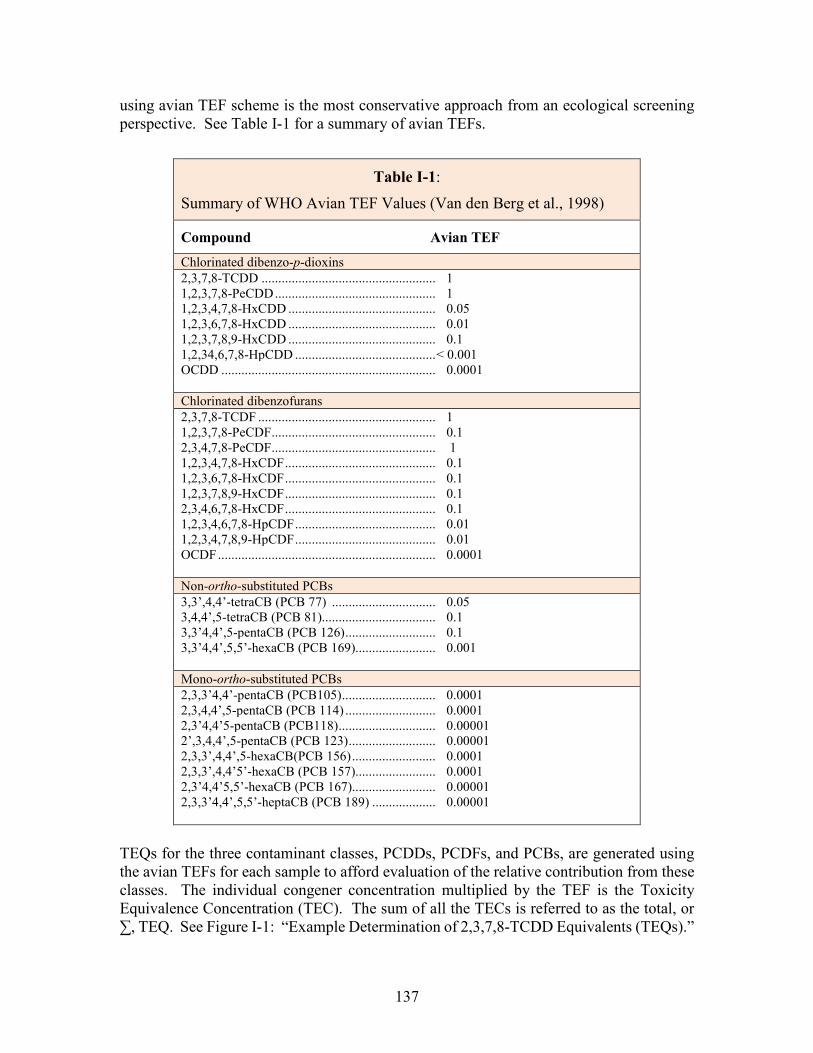
137
using avian TEF scheme is the most conservative approach from an ecological screening perspective. See Table I-1 for a summary of avian TEFs.
Table I-1:
Summary of WHO Avian TEF Values (Van den Berg et al., 1998)
Compound Avian TEF Chlorinated dibenzo-p-dioxins 2,3,7,8-TCDD .................................................... 1 1,2,3,7,8-PeCDD ................................................ 1 1,2,3,4,7,8-HxCDD ............................................ 0.05 1,2,3,6,7,8-HxCDD ............................................ 0.01 1,2,3,7,8,9-HxCDD ............................................ 0.1 1,2,34,6,7,8-HpCDD .......................................... < 0.001 OCDD ................................................................ 0.0001 Chlorinated dibenzofurans 2,3,7,8-TCDF ..................................................... 1 1,2,3,7,8-PeCDF ................................................. 0.1 2,3,4,7,8-PeCDF ................................................. 1 1,2,3,4,7,8-HxCDF ............................................. 0.1 1,2,3,6,7,8-HxCDF ............................................. 0.1 1,2,3,7,8,9-HxCDF ............................................. 0.1 2,3,4,6,7,8-HxCDF ............................................. 0.1 1,2,3,4,6,7,8-HpCDF .......................................... 0.01 1,2,3,4,7,8,9-HpCDF .......................................... 0.01 OCDF ................................................................. 0.0001 Non-ortho-substituted PCBs 3,3’,4,4’-tetraCB (PCB 77) ............................... 0.05 3,4,4’,5-tetraCB (PCB 81).................................. 0.1 3,3’4,4’,5-pentaCB (PCB 126) ........................... 0.1 3,3’4,4’,5,5’-hexaCB (PCB 169)........................ 0.001 Mono-ortho-substituted PCBs 2,3,3’4,4’-pentaCB (PCB105) ............................ 0.0001 2,3,4,4’,5-pentaCB (PCB 114) ........................... 0.0001 2,3’4,4’5-pentaCB (PCB118) ............................. 0.00001 2’,3,4,4’,5-pentaCB (PCB 123) .......................... 0.00001 2,3,3’,4,4’,5-hexaCB(PCB 156) ......................... 0.0001 2,3,3’,4,4’5’-hexaCB (PCB 157)........................ 0.0001 2,3’4,4’5,5’-hexaCB (PCB 167)......................... 0.00001 2,3,3’4,4’,5,5’-heptaCB (PCB 189) ................... 0.00001
TEQs for the three contaminant classes, PCDDs, PCDFs, and PCBs, are generated using the avian TEFs for each sample to afford evaluation of the relative contribution from these classes. The individual congener concentration multiplied by the TEF is the Toxicity Equivalence Concentration (TEC). The sum of all the TECs is referred to as the total, or ∑, TEQ. See Figure I-1: “Example Determination of 2,3,7,8-TCDD Equivalents (TEQs).”
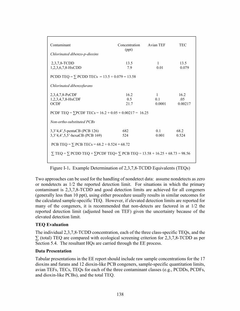
138
Figure I-1. Example Determination of 2,3,7,8-TCDD Equivalents (TEQs) Two approaches can be used for the handling of nondetect data: assume nondetects as zero or nondetects as 1/2 the reported detection limit. For situations in which the primary contaminant is 2,3,7,8-TCDD and good detection limits are achieved for all congeners (generally less than 10 ppt), using either procedure usually results in similar outcomes for the calculated sample-specific TEQ. However, if elevated detection limits are reported for many of the congeners, it is recommended that non-detects are factored in at 1/2 the reported detection limit (adjusted based on TEF) given the uncertainty because of the elevated detection limit.
TEQ Evaluation The individual 2,3,7,8-TCDD concentration, each of the three class-specific TEQs, and the ∑ (total) TEQ are compared with ecological screening criterion for 2,3,7,8-TCDD as per Section 5.4. The resultant HQs are carried through the EE process.
Data Presentation Tabular presentations in the EE report should include raw sample concentrations for the 17 dioxins and furans and 12 dioxin-like PCB congeners, sample-specific quantitation limits, avian TEFs, TECs, TEQs for each of the three contaminant classes (e.g., PCDDs, PCDFs, and dioxin-like PCBs), and the total TEQ.
Contaminant Concentration Avian TEF TEC (ppt) Chlorinated dibenzo-p-dioxins 2,3,7,8-TCDD 13.5 1 13.5 1,2,3,6,7,8-HxCDD 7.9 0.01 0.079 PCDD TEQ = ∑ PCDD TECs = 13.5 + 0.079 = 13.58 Chlorinated dibenzofurans 2,3,4,7,8-PeCDF 16.2 1 16.2 1,2,3,4,7,8-HxCDF 0.5 0.1 .05 OCDF 21.7 0.0001 0.00217 PCDF TEQ = ∑PCDF TECs = 16.2 + 0.05 + 0.00217 = 16.25 Non-ortho-substituted PCBs 3,3’4,4’,5-pentaCB (PCB 126) 682 0.1 68.2 3,3’4,4’,5,5’-hexaCB (PCB 169) 524 0.001 0.524
PCB TEQ = ∑ PCB TECs = 68.2 + 0.524 = 68.72
∑ TEQ = ∑ PCDD TEQ + ∑PCDF TEQ+ ∑ PCB TEQ = 13.58 + 16.25 + 68.73 = 98.56

139
Evaluation of Dioxins, Furans, and Dioxin-like PCBs in the Ecological Risk Assessment The investigator is referred to USEPA 1993b and USEPA 2008b regarding ecological risk characterization approaches and the application of the TEQ process to tissue concentrations and food chain modeling.