Chapter 5: Probability Distributions: Discrete Probability Distributions

ECO220YDiscrete Probability Distributions:
Bernoulli and BinomialReadings: Chapter 9, Sections 9.4 and 9.6 only
Fall 2011
Lecture 7
(Fall 2011) Probability Distributions Lecture 7 1 / 28
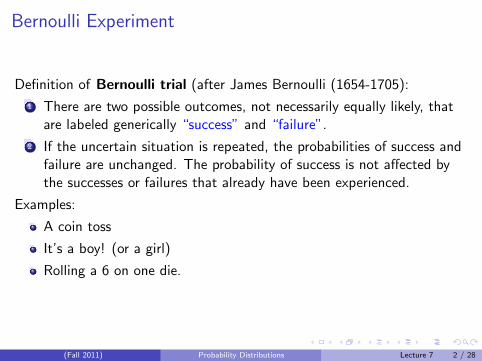
Bernoulli Experiment
Definition of Bernoulli trial (after James Bernoulli (1654-1705):
1 There are two possible outcomes, not necessarily equally likely, thatare labeled generically “success” and “failure”.
2 If the uncertain situation is repeated, the probabilities of success andfailure are unchanged. The probability of success is not affected bythe successes or failures that already have been experienced.
Examples:
A coin toss
It’s a boy! (or a girl)
Rolling a 6 on one die.
(Fall 2011) Probability Distributions Lecture 7 2 / 28

Bernoulli Random Variable
Bernoulli random variable records an outcome of Bernoulli experiment.
x P(X=x)
0 (failure) 1-p
1 (success) p
E [X ] = 1 ∗ p + 0 ∗ (1− p) = p
V [X ] = (1− p)2 ∗ p + (0− p)2 ∗ (1− p) = p ∗ (1− p)
E [X ] = µ = p and V [X ] = σ2 = p ∗ (1− p)
Bernoulli - discrete or continuous RV?
(Fall 2011) Probability Distributions Lecture 7 3 / 28

Binomial Experiment
1 There are two possible outcomes, not necessarily equally likely, thatare labeled generically “success” and “failure”.
2 If the uncertain situation is repeated, the probabilities of success andfailure are unchanged. The probability of success is not affected bythe successes or failures that already have been experienced.
3 We have a sequence of Bernoulli trials.
(Fall 2011) Probability Distributions Lecture 7 4 / 28

Binomial Random Variable
Binomial random variable counts the number of successes in aBinomial experiment.
Binomial distribution returns probability of each possible value ofbinomial random variable X.
Examples:
A number of heads in a series of 5 coin tosses.
A number of boys in families with three children.
(Fall 2011) Probability Distributions Lecture 7 5 / 28

Probability Tree
(Fall 2011) Probability Distributions Lecture 7 6 / 28

Probability distribution
x P(x)
0 0.125
1 0.375
2 0.375
3 0.125
Total 1
=⇒
Which probability ruleshave we used to derive
this probability distribution?
(Fall 2011) Probability Distributions Lecture 7 7 / 28
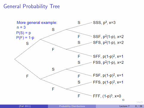
General Probability Tree
(Fall 2011) Probability Distributions Lecture 7 8 / 28
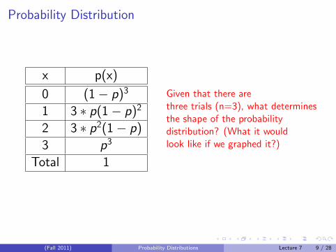
Probability Distribution
x p(x)
0 (1− p)3
1 3 ∗ p(1− p)2
2 3 ∗ p2(1− p)
3 p3
Total 1
Given that there arethree trials (n=3), what determinesthe shape of the probabilitydistribution? (What it wouldlook like if we graphed it?)
(Fall 2011) Probability Distributions Lecture 7 9 / 28
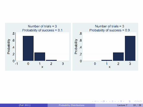
(Fall 2011) Probability Distributions Lecture 7 10 / 28

When p=.5, the binomial probability distribution is perfectly symmetrical.For 6 coin flips, for instance, it is:
x 0 1 2 3 4 5 6
P(x) 12
6 12
6 ∗ 6 12
6 ∗ 15 12
6 ∗ 20 12
6 ∗ 15 12
6 ∗ 6 12
6
(Fall 2011) Probability Distributions Lecture 7 11 / 28

What if n is large?If n (number of trials) in binomial experiment is large, we can compute theprobabilities for all of the possible values of X as:
P(x successes) = P(x) = Cnx px(1− p)n−x
where Cnx is number of all possible sequences with x successes:
Cnx = n!
x!(n−x)!
n! = n ∗ (n − 1) ∗ (n − 2) ∗ (n − 3) ∗ ...3 ∗ 2 ∗ 1
Cnn = Cn
0 = 1, Cnx = Cn
n−x , 0! = 1, 1! = 1
Note: C nx is the binomial coefficient, read ”n choose x”
(Fall 2011) Probability Distributions Lecture 7 12 / 28
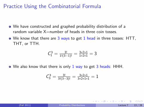
Practice Using the Combinatorial Formula
We have constructed and graphed probability distribution of arandom variable X=number of heads in three coin tosses.
We know that there are 3 ways to get 1 head in three tosses: HTT,THT, or TTH.
C 31 = 3!
1!(3−1)!= 3∗2∗1
1∗2∗1 = 3
We also know that there is only 1 way to get 3 heads: HHH.
C 33 = 3!
3!(3−3)!= 3∗2∗1
3∗2∗1∗1 = 1
(Fall 2011) Probability Distributions Lecture 7 13 / 28

Combinatorial Formula The Easy Way
C 1611 = 16!
11!5! = 16·15·14·13·12·
11!︷ ︸︸ ︷11 · ... · 1
(11 · ... · 1)︸ ︷︷ ︸11!
∗(5·4·3·2·1)= 16·15·14·13·12
5·4·3·2·1
(Fall 2011) Probability Distributions Lecture 7 14 / 28

Binomial Probability Distribution
To describe binomial distribution, we need two parameters: n and p. Thebinomial distribution states that, in n Bernoulli trials, with probability p ofsuccess on each trial, the probability of exactly x successes is:
P(X = x) = C nx ∗ px(1− p)n−x = n!
x!(n−x)!px(1− p)n−x
(Fall 2011) Probability Distributions Lecture 7 15 / 28

(Fall 2011) Probability Distributions Lecture 7 16 / 28
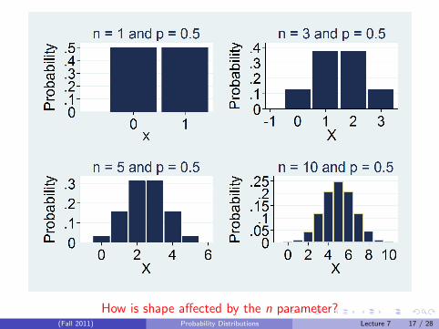
How is shape affected by the n parameter?(Fall 2011) Probability Distributions Lecture 7 17 / 28

How is shape affected by the p parameter?(Fall 2011) Probability Distributions Lecture 7 18 / 28

How is shape affected by the n parameter?(Fall 2011) Probability Distributions Lecture 7 19 / 28

Expected Value and Variance of Binomial RV
Binomial RV is a sum of Bernoulli RVsWhich laws we are going to use to find µ and σ2?
Y =n∑
i=1
Xi
where n is a number of Bernoulli trials and E [X ] = p and V [X ] = p(1− p)
E [Y ] = E [n∑
i=1
Xi ] = E [nXi ] = n ∗ E [Xi ] = np
V [Y ] = V [n∑
i=1
Xi ] =n∑
i=1
V [Xi ] = nV [Xi ] = np(1− p)
(Fall 2011) Probability Distributions Lecture 7 20 / 28

Summary
Binomial distribution is described by two parameters: n and p
Shape of the probability distribution for binomial RV depends onparameters
For any p and n we can find the probability of obtaining x successesin n trials as P(X = x) = Cn
x px(1− p)n−x
E [X ] = µ = np
V [X ] = σ2 = np(1− p)
(Fall 2011) Probability Distributions Lecture 7 21 / 28

Example
The Adams are planning their family and both want an equal number ofboys and girls. Mrs Adams says their chances are best if they plan onhaving two children. Mr Adams says that they have a better chance ofhaving an equal number of boys and girls if they plan on having fourchildren. Who is right? (Let’s assume that boy and girl babies are equallylikely)
(Fall 2011) Probability Distributions Lecture 7 22 / 28

Statistically Plausible?
Statistics Professor claims that 90% of the students are extremely satisfiedwith the course he is teaching. We randomly sample 5 students to findthat only 1 student is actually ”extremely satisfied”. Is this resultstatistically plausible given that the claim is true?
(Fall 2011) Probability Distributions Lecture 7 23 / 28
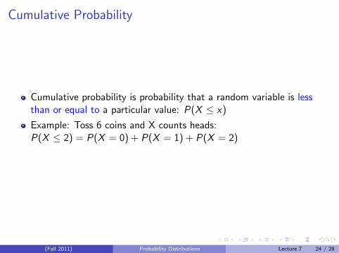
Cumulative Probability
Cumulative probability is probability that a random variable is lessthan or equal to a particular value: P(X ≤ x)
Example: Toss 6 coins and X counts heads:P(X ≤ 2) = P(X = 0) + P(X = 1) + P(X = 2)
(Fall 2011) Probability Distributions Lecture 7 24 / 28
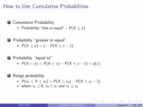
How to Use Cumulative Probabilities
1 Cumulative ProbabilityI Probability “less or equal” - P(X ≤ x)
2 Probability “greater or equal”I P(X ≥ x) = 1− P(X ≤ x − 1)
3 Probability “equal to”I P(X = x) = P(X ≤ x)− P(X ≤ x − 1) = p(x)
4 Range probabilityI P(x1 ≤ X ≤ x2) = P(X ≤ x2)− P(X ≤ x1 − 1)I where x1 ≥ 0, x2 ≤ n, and x1 ≤ x2
(Fall 2011) Probability Distributions Lecture 7 25 / 28

Example
Consider binomial distribution with p=.5 and n=100
P(X ≤ 50) = 0.5397
P(X ≥ 65) = 1− P(X ≤ 65− 1) = 1− P(X ≤ 64) = 1− 0.9982 =0.0018
P(X = 45) = P(X ≤ 45)− P(X ≤ 44) = 0.1841− 0.1356 = 0.0485
P(45 ≤ X ≤ 55) = P(X ≤ 55)− P(X ≤ 44) = 0.8643− 0.1356 =0.7287
(Fall 2011) Probability Distributions Lecture 7 26 / 28
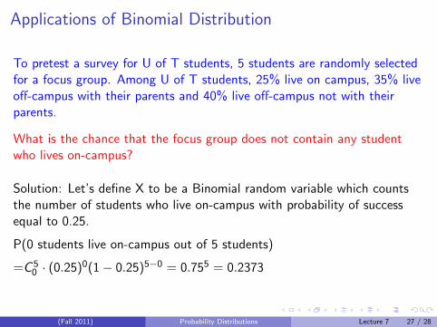
Applications of Binomial Distribution
To pretest a survey for U of T students, 5 students are randomly selectedfor a focus group. Among U of T students, 25% live on campus, 35% liveoff-campus with their parents and 40% live off-campus not with theirparents.
What is the chance that the focus group does not contain any studentwho lives on-campus?
Solution: Let’s define X to be a Binomial random variable which countsthe number of students who live on-campus with probability of successequal to 0.25.
P(0 students live on-campus out of 5 students)
=C 50 · (0.25)0(1− 0.25)5−0 = 0.755 = 0.2373
(Fall 2011) Probability Distributions Lecture 7 27 / 28

What is the chance that more than two-thirds of the focus group isstudents who live off-campus not with their parents?
Solution: Let’s define X to be a Binomial random variable which countsthe number of students who live off-campus not with their parents withprobability 0.4. Two-thirds of 5 is 3, not 3.(3). “More than two-thirds”means 4 or 5 students. We need to find P(X>3)=P(X=4) + P(X=5).
P(X=4)+P(X=5)=C 54 · (0.4)4(1− 0.4)1 + C 5
5 · 0.45(1− 0.4)0
=0.078+0.0102=0.087
(Fall 2011) Probability Distributions Lecture 7 28 / 28