ECN741: Urban Economics More General Treatment of Housing Demand.
Upload
earl-simmonsCategory
view
219download
1
ECN741: Urban Economics
Multiple Worksites and Full Labor Markets
Multiple Worksites
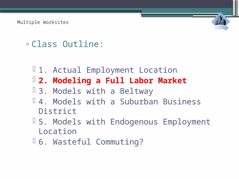
▫Class Outline:
1. Actual Employment Location 2. Modeling a Full Labor Market 3. Models with a Beltway 4. Models with a Suburban Business District 5. Models with Endogenous Employment
Location 6. Wasteful Commuting?

Multiple Worksites
▫Class Outline:
1. Actual Employment Location 2. Modeling a Full Labor Market 3. Models with a Beltway 4. Models with a Suburban Business District 5. Models with Endogenous Employment
Location 6. Wasteful Commuting?
Multiple Worksites
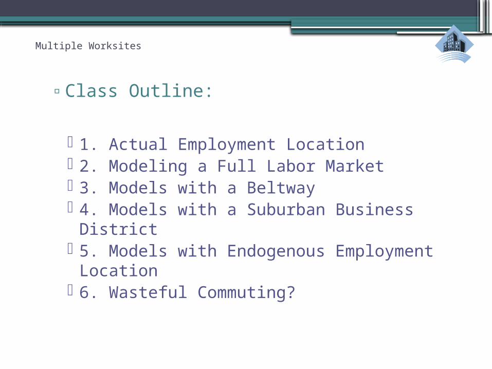
Defining Worksites
• Worksites can be identified using data on the number of jobs within each zip code, which is available from the census.
• The definition of a worksite considers both the concentration of jobs in a core zip code and the clustering of jobs in related zip codes.
• In my study of Cleveland, which is similar to others, a worksite is defined as a set of zip codes
▫ each with at least 5,000 jobs
▫ that contain at least one zip code with 25,000 jobs,
▫ that contain at least 45,000 total jobs
▫ and that are all within 6 miles of a central point.
Multiple Worksites
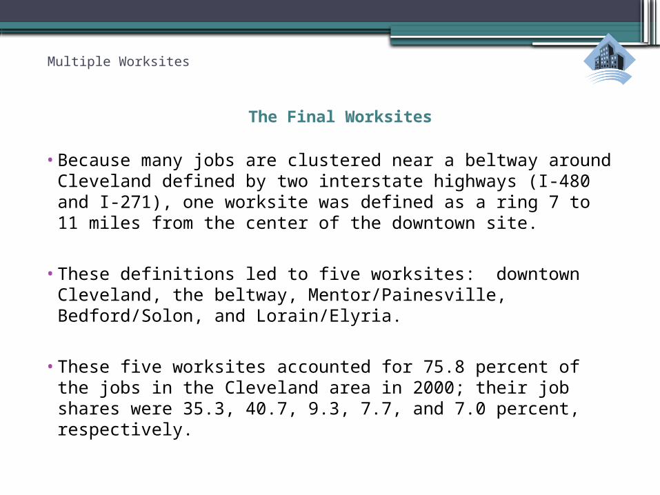
The Final Worksites
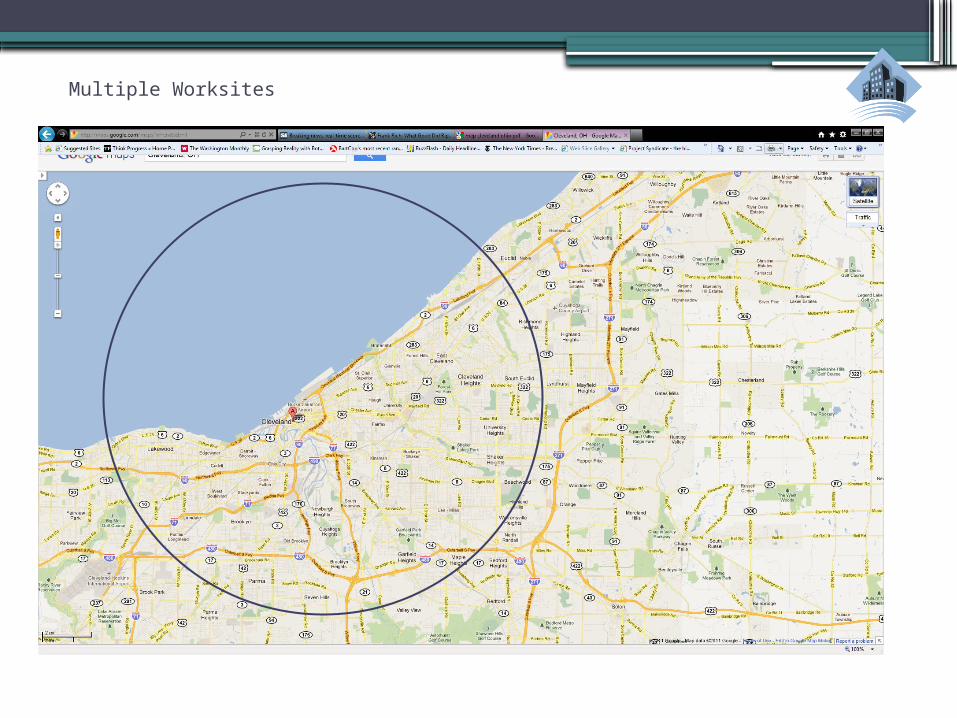
• Because many jobs are clustered near a beltway around Cleveland defined by two interstate highways (I-480 and I-271), one worksite was defined as a ring 7 to 11 miles from the center of the downtown site.
• These definitions led to five worksites: downtown Cleveland, the beltway, Mentor/Painesville, Bedford/Solon, and Lorain/Elyria.
• These five worksites accounted for 75.8 percent of the jobs in the Cleveland area in 2000; their job shares were 35.3, 40.7, 9.3, 7.7, and 7.0 percent, respectively.

Multiple Worksites
-82.5 -82.3 -82.1 -81.9 -81.7 -81.5 -81.3 -81.1 -80.9 -80.740.9
41
41.1
41.2
41.3
41.4
41.5
41.6
41.7
41.8
41.9
Block Group Downtown BeltwayBedford/Solon Lorain/Elyria Mentor/Painesville
Longitude
Lati
tude
Multiple Worksites
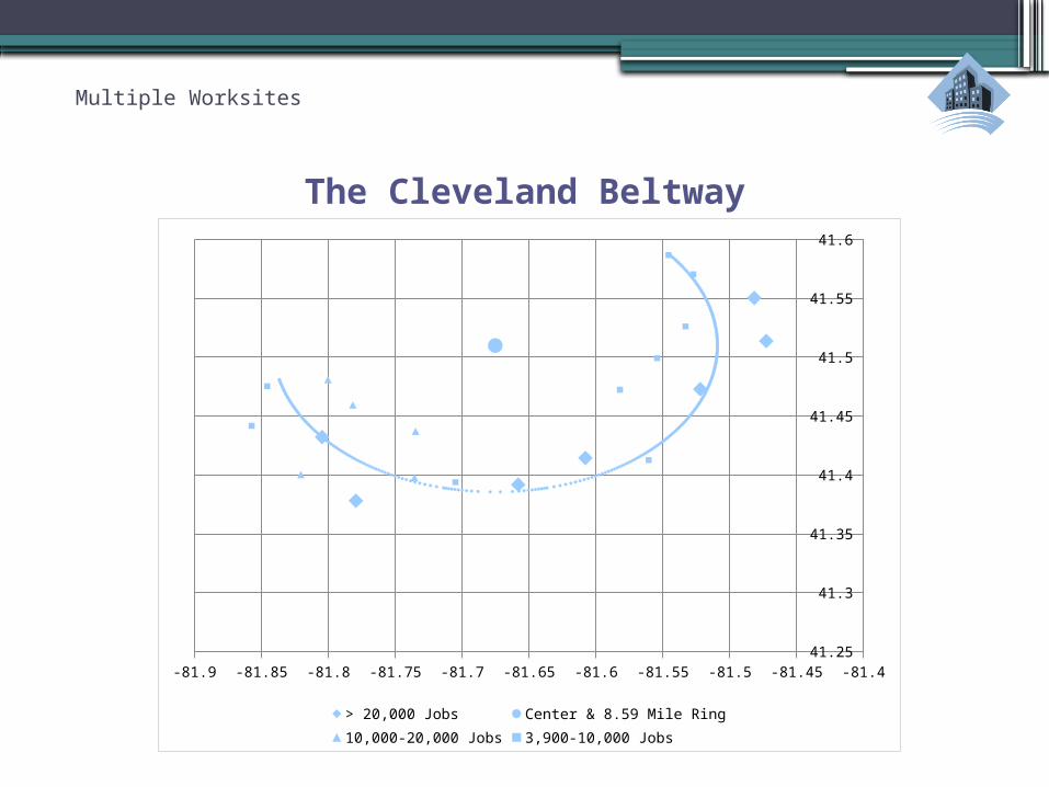
The Cleveland Beltway
-81.9 -81.85 -81.8 -81.75 -81.7 -81.65 -81.6 -81.55 -81.5 -81.45 -81.441.25
41.3
41.35
41.4
41.45
41.5
41.55
41.6
> 20,000 Jobs Center & 8.59 Mile Ring10,000-20,000 Jobs 3,900-10,000 Jobs
Multiple Worksites
Multiple Worksites
▫Class Outline:
1. Actual Employment Location 2. Modeling a Full Labor Market 3. Models with a Beltway 4. Models with a Suburban Business District 5. Models with Endogenous Employment
Location 6. Wasteful Commuting?
Multiple Worksites
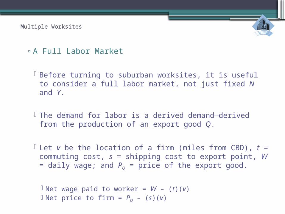
▫A Full Labor Market
Before turning to suburban worksites, it is useful to consider a full labor market, not just fixed N and Y.
The demand for labor is a derived demand—derived from the production of an export good Q.
Let v be the location of a firm (miles from CBD), t = commuting cost, s = shipping cost to export point, W = daily wage; and PQ = price of the export good.
Net wage paid to worker = W – (t)(v) Net price to firm = PQ – (s)(v)
Multiple Worksites
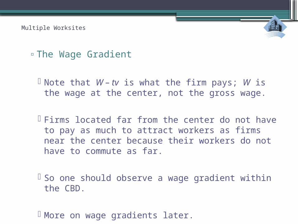
▫The Wage Gradient
Note that W – tv is what the firm pays; W is the wage at the center, not the gross wage.
Firms located far from the center do not have to pay as much to attract workers as firms near the center because their workers do not have to commute as far.
So one should observe a wage gradient within the CBD.
More on wage gradients later.

Multiple Worksites
The CBD Boundary
R{u}
Rf
Rh
u
_uu
_R
Multiple Worksites
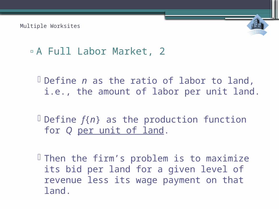
▫A Full Labor Market, 2
Define n as the ratio of labor to land, i.e., the amount of labor per unit land.
Define f{n} as the production function for Q per unit of land.
Then the firm’s problem is to maximize its bid per land for a given level of revenue less its wage payment on that land.
Multiple Worksites
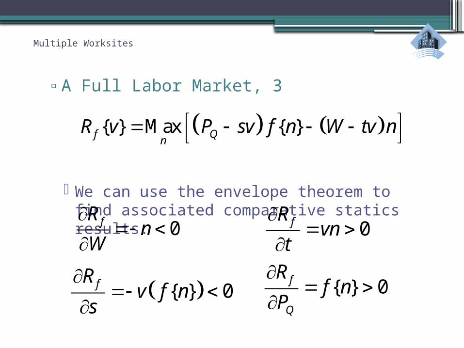
▫A Full Labor Market, 3
We can use the envelope theorem to find associated comparative statics results:
{ } Max { }f Qn
R v P sv f n W tv n
0fRn
W
0fR
vnt
{ } 0fRv f n
s
{ } 0f
Q
Rf n
P
Multiple Worksites
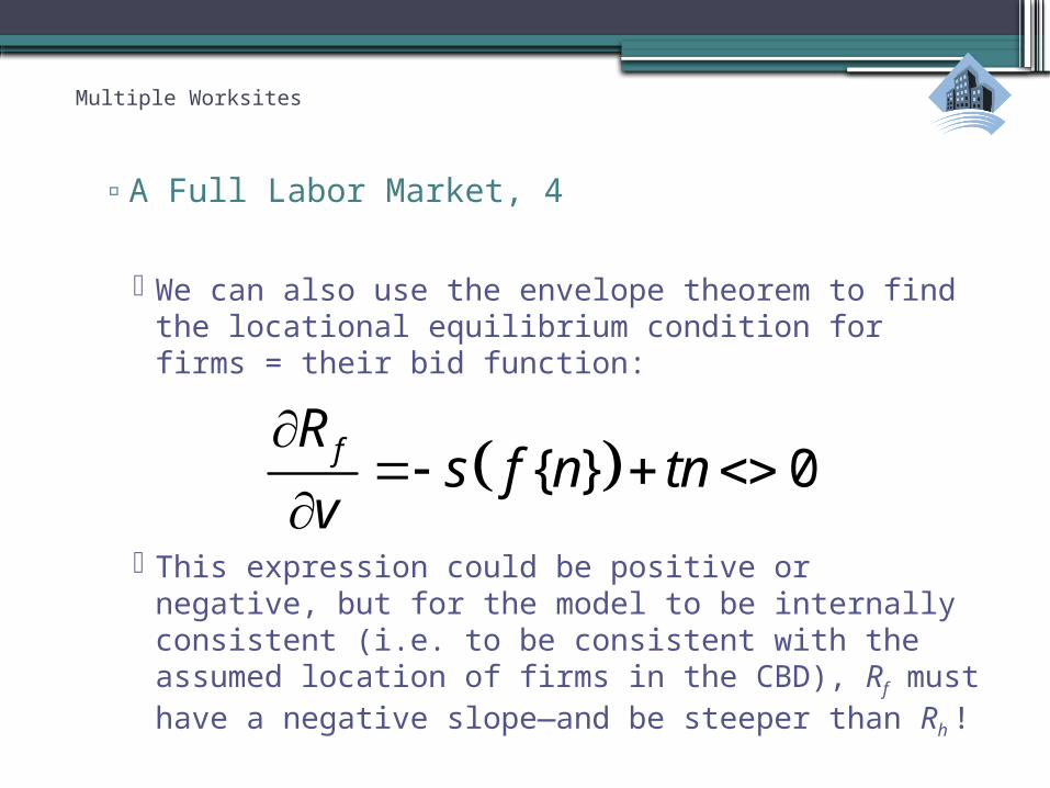
▫A Full Labor Market, 4
We can also use the envelope theorem to find the locational equilibrium condition for firms = their bid function:
This expression could be positive or negative, but for the model to be internally consistent (i.e. to be consistent with the assumed location of firms in the CBD), Rf must have a negative slope—and be steeper than Rh !
{ } 0fRs f n tn
v
Multiple Worksites
▫A Full Labor Market, 5
Ross and Yinger (RSUE, 1995) use these and other results to obtain the comparative statics tables for an open urban model with a full labor market.
Most of the comparative statics results do not hold up when a full labor market is added—primarily because of role played by the CBD boundary.
They conclude that “the determinacy of many comparative statics results in the standard open urban model depends on the unrealistic assumption of perfectly elastic labor demand.”
Multiple Worksites
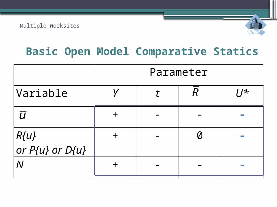
Basic Open Model Comparative Statics
Parameter
Variable Y t U*
+ - - -
R{u}or P{u} or D{u}
+ - 0 -
N + - - -
R
u
Multiple Worksites
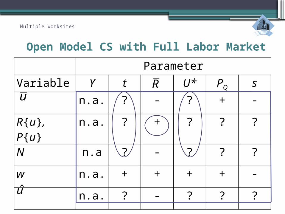
Open Model CS with Full Labor Market
Parameter
Variable Y t U* PQ s
n.a. ? - ? + -
R{u}, P{u} n.a. ? + ? ? ?
N n.a ? - ? ? ?
w n.a. + + + + -
n.a. ? - ? ? ?
Ru
u
Multiple Worksites
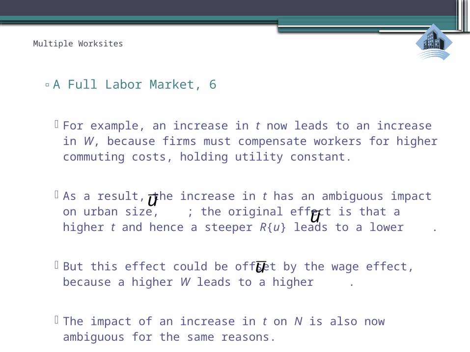
▫A Full Labor Market, 6
For example, an increase in t now leads to an increase in W, because firms must compensate workers for higher commuting costs, holding utility constant.
As a result, the increase in t has an ambiguous impact on urban size, ; the original effect is that a higher t and hence a steeper R{u} leads to a lower .
But this effect could be offset by the wage effect, because a higher W leads to a higher .
The impact of an increase in t on N is also now ambiguous for the same reasons.
u
u
u
Multiple Worksites
▫Class Outline:
1. Actual Employment Location 2. Modeling a Full Labor Market 3. Models with a Beltway 4. Models with a Suburban Business District 5. Models with Endogenous Employment
Location 6. Wasteful Commuting?
Multiple Worksites
▫The White Beltway Model
White (JUE, 1976) introduced a beltway a given distance from the CBD (but no full labor market).
This keeps the model monocentric and the math tractable. A second beltway could be added.
It provides a rough approximation to the employment distribution in some urban areas.
Multiple Worksites
R{u}
u
_R
_ubu*
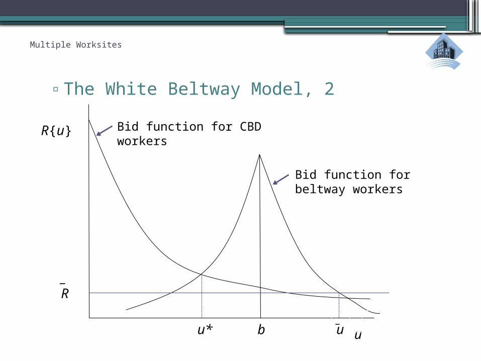
▫The White Beltway Model, 2
Bid function for CBD workers
Bid function for beltway workers
Multiple Worksites
▫The White Beltway Model, 3
So this model, like the two-class model, has sorting, now between the residential zones of CBD and beltway workers.
It has a new variable, u*, the zone boundary.
If workers are mobile across worksites, the bid-function peaks must have the same height.
It is theoretically possible for CBD workers to commute through the beltway workers’ zone.
Multiple Worksites
▫The White Beltway Model, 4
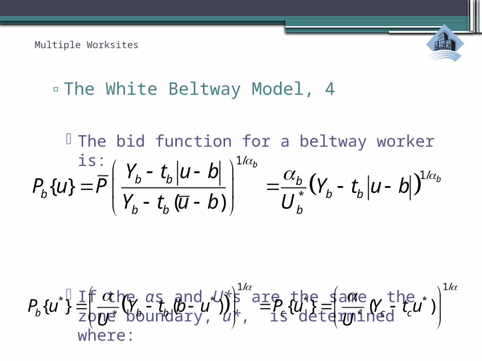
The bid function for a beltway worker is:
If the αs and U*s are the same, the zone boundary, u*, is determined where:
1/
1/
*{ }
( )
b
bb b bb b b
b b b
Y t u bP u P Y t u b
Y t u b U
1/ 1/
* * * ** *
{ } ( ) { } ( )b b b c c cP u Y t b u P u Y t uU U
Multiple Worksites
▫The White Beltway Model, 4
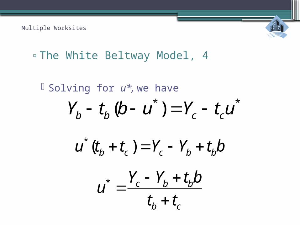
Solving for u*, we have
* *( )b b c cY t b u Y t u
*( )b c c b bu t t Y Y t b
* c b b
b c
Y Y t bu
t t
Multiple Worksites
▫The White Beltway Model, 4
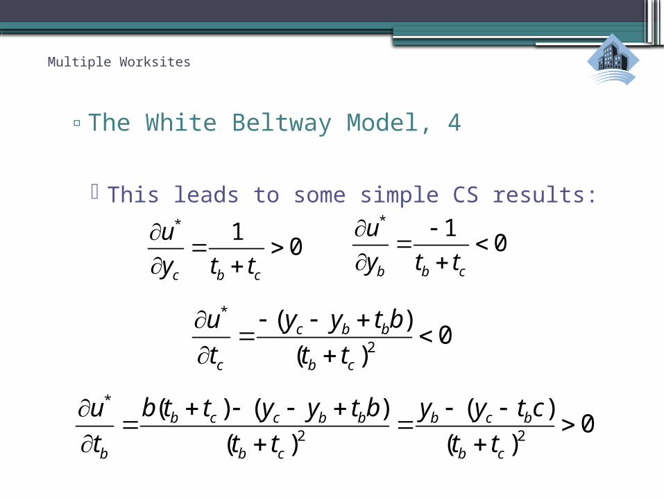
This leads to some simple CS results:
* 10
c b c
u
y t t
* 10
b b c
u
y t t
*
2 2
( ) ( ) ( )0
( ) ( )b c c b b b c b
b b c b c
b t t y y t b y y t cu
t t t t t
*
2
( )0
( )c b b
c b c
y y t bu
t t t

Multiple Worksites
▫The White Beltway Model, 4
Finally, the population integrals in a beltway model look like this:
*
( )u
c c
o
N N u du
*
( ) ( )b u
b b b
bu
N N b u du N u b du
Multiple Worksites
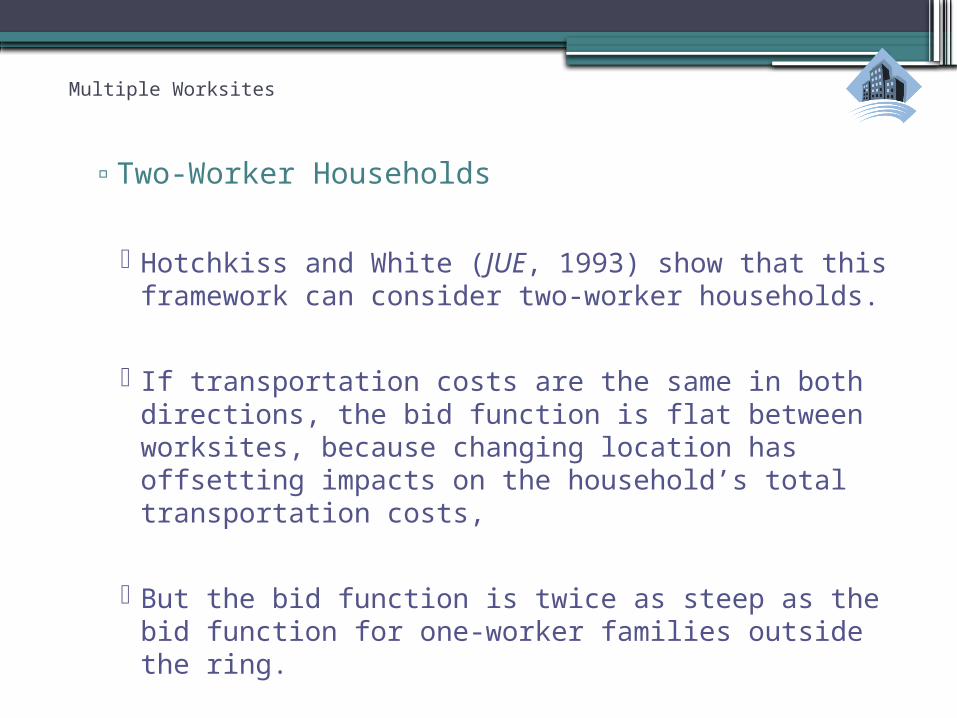
▫Two-Worker Households
Hotchkiss and White (JUE, 1993) show that this framework can consider two-worker households.
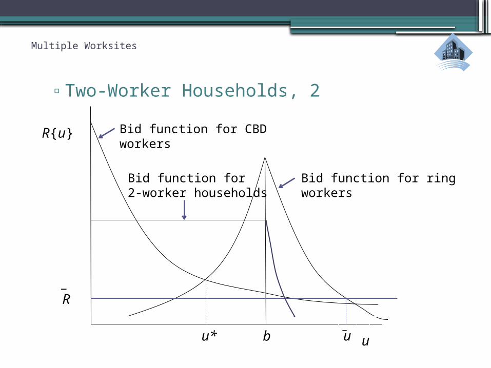
If transportation costs are the same in both directions, the bid function is flat between worksites, because changing location has offsetting impacts on the household’s total transportation costs,
But the bid function is twice as steep as the bid function for one-worker families outside the ring.
Multiple Worksites
R{u}
u
_R
_ubu*
▫Two-Worker Households, 2
Bid function for CBD workers
Bid function for ring workers
Bid function for2-worker households
Multiple Worksites
▫Class Outline:
1. Actual Employment Location 2. Modeling a Full Labor Market 3. Models with a Beltway 4. Models with a Suburban Business
District 5. Models with Endogenous Employment
Location 6. Wasteful Commuting?

Multiple Worksites
▫Models of Suburban Business Districts
Several scholars have modeled urban areas with SBDs at a particular point, which means they models are no longer monocentric.
The models assume the SBD is at a given location; they do not determine this location endogenously.
Many different assumptions about the street networks have been used.
Multiple Worksites
▫Models of Suburban Business Districts
Wieand (JUE, 1987): assumes radial streets out of CBD and SBD; shows that the zone boundary is a hyperbola; cannot solve population integral.
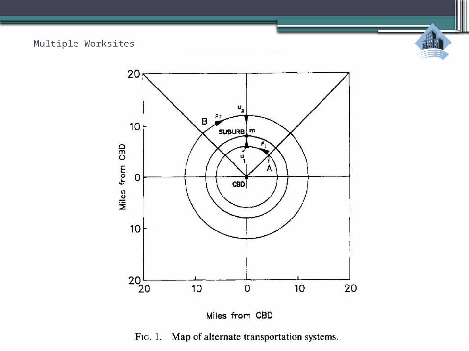
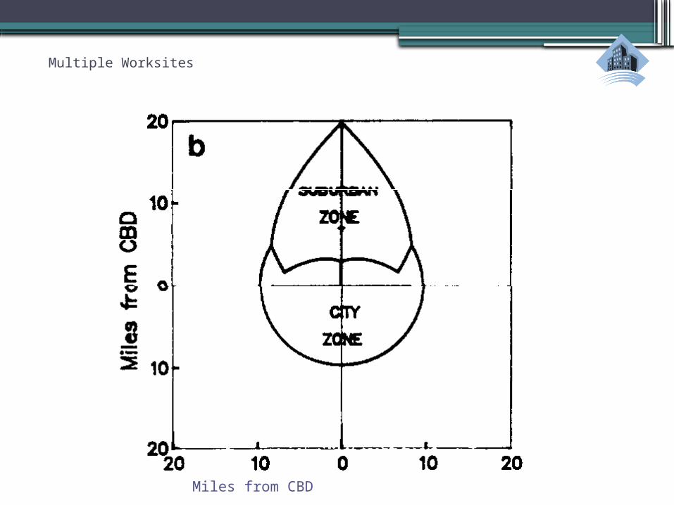
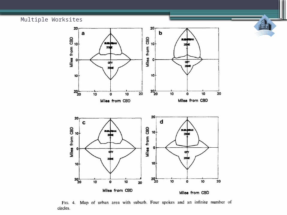
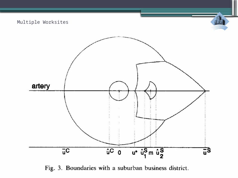
Yinger (JUE, 1992): assumes radial arteries and circular streets; solves for the shapes of CBD and SBD residential zones. (See the next two slides.)
Yinger (JUE, 1993): assumes a street grid plus, in come cases, arteries; solves for the shapes of CBD and SBD residential zones.
Multiple Worksites
Multiple Worksites
Miles from CBD
Multiple Worksites
▫“City and Suburb”
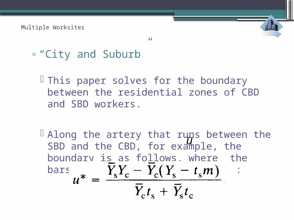
This paper solves for the boundary between the residential zones of CBD and SBD workers.
Along the artery that runs between the SBD and the CBD, for example, the boundary is as follows, where the bars indicate net incomes at :
u
Multiple Worksites
▫“City and Suburb,” 2
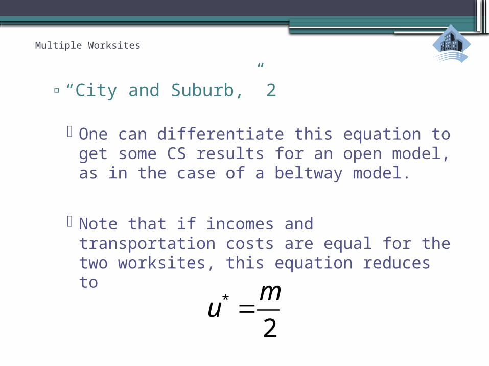
One can differentiate this equation to get some CS results for an open model, as in the case of a beltway model.
Note that if incomes and transportation costs are equal for the two worksites, this equation reduces to
*
2
mu
Multiple Worksites
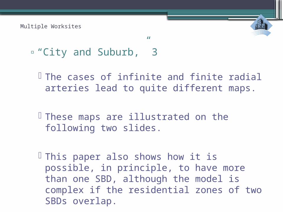
▫“City and Suburb,” 3
The cases of infinite and finite radial arteries lead to quite different maps.
These maps are illustrated on the following two slides.
This paper also shows how it is possible, in principle, to have more than one SBD, although the model is complex if the residential zones of two SBDs overlap.

Multiple Worksites
Multiple Worksites
Multiple Worksites
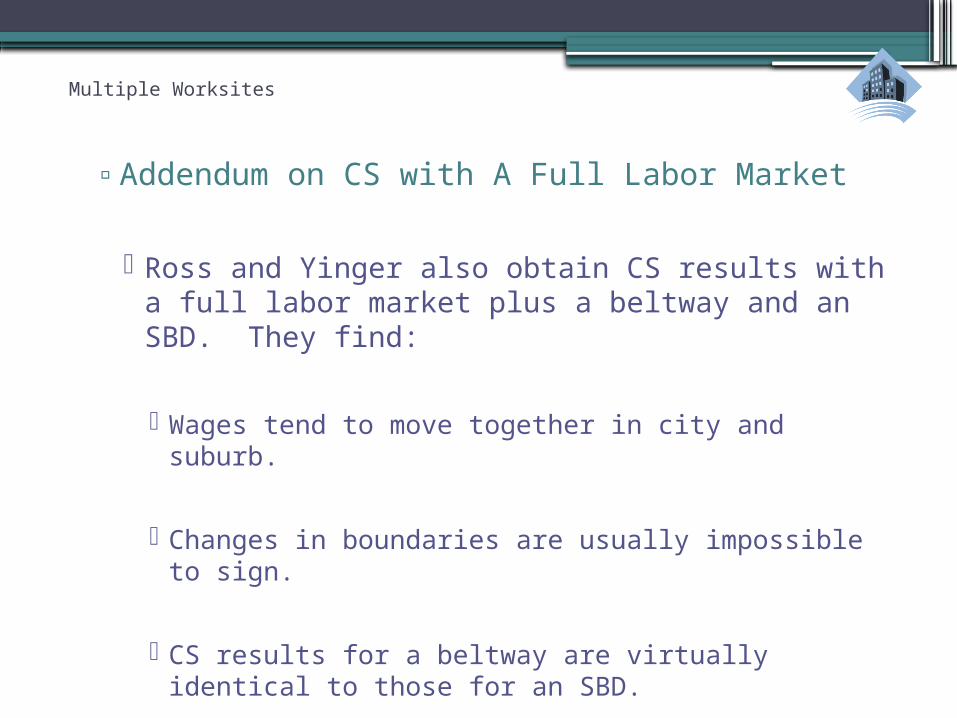
▫Addendum on CS with A Full Labor Market
Ross and Yinger also obtain CS results with a full labor market plus a beltway and an SBD. They find:
Wages tend to move together in city and suburb.
Changes in boundaries are usually impossible to sign.
CS results for a beltway are virtually identical to those for an SBD.
Multiple Worksites
Multiple Worksites
▫Class Outline:
1. Actual Employment Location 2. Modeling a Full Labor Market 3. Models with a Beltway 4. Models with a Suburban Business District 5. Models with Endogenous Employment
Location 6. Wasteful Commuting?
Multiple Worksites
▫Endogenous Employment Location
An important question that is difficult to answer is: Why do SBDs arise where they do?
To some degree, the answer may be about historical events or political decisions, such as where to build a beltway.
But there are economic incentives, too.

Multiple Worksites
▫Endogenous Employment Location, 2
As discussed in the White Handbook chapter, firms may be able to save money by moving from a CBD to an SBD.
The savings arises because they can save workers commuting costs—and hence pay them lower wages.
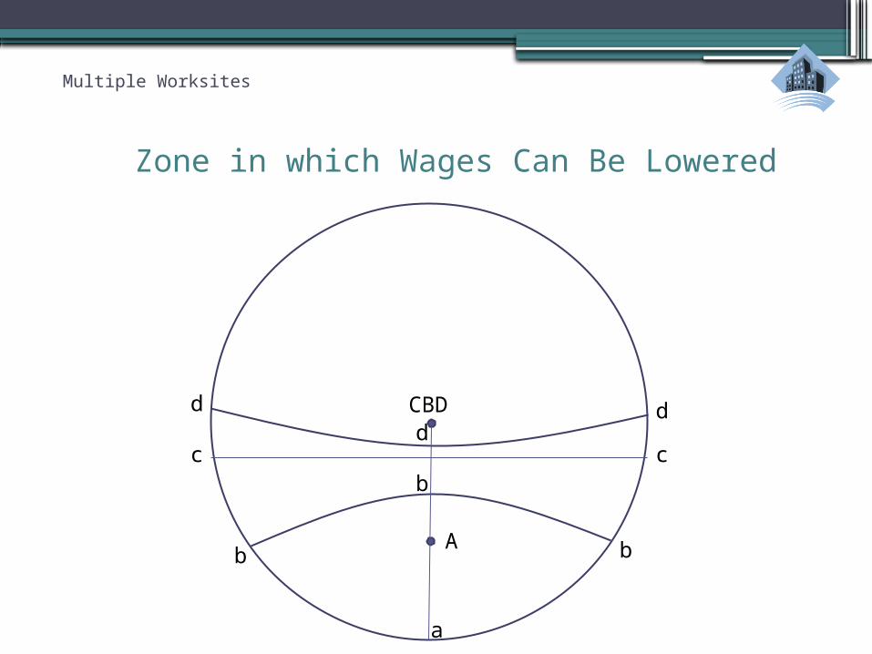
In the following picture, a firm that locates at A saves commuting costs equal to the distance between A and the CBD for all workers outside A on the artery between the CBD and A.
If it raises wages, it picks up workers outside some arc, such as bbb (or, with equal wages, cc, and with higher wages, ddd).
Multiple Worksites
Zone in which Wages Can Be Lowered
CBD
Ab
b
b
c
dd
d
c
a
Multiple Worksites
▫Other Factors in Firm Location
Many other hard-to-model factors might influence the emergence of an SBD, or course, such as:
Agglomeration economies (i.e. productivity advantages from being near other firms);
Access to transportation; Access to productivity-related amenities or
public services; Access to certain types of workers; Distance from competitors.
Multiple Worksites
▫Solving for Employment Locations
An amazing article by Lucas and Rossi-Hansberg (Econometrica, 2002) solves for the equilibrium location of export employment in a monocentric city.
Employment can be in any ring, and some rings might have an employment/housing mix.
Labor productivity can be influenced by employment in nearby rings.
The mathematics is advanced!
Multiple Worksites
▫Local Employment and the Wage Gradient
Brueckner (JUE, 1979), introduces local employment, which consists of jobs in dry cleaners, fast-food restaurants, and so on.
These jobs serve residents where they live—so they follow people.
The price of housing is determined by commuters to the CBD, so local market workers have to be “uncompensated” at distant locations by receiving a lower wage rate—generating a wage gradient.
Multiple Worksites
▫The Wage Gradient
There is a large empirical literature on wage gradients.
See, for example, Timothy and Wheaton (JUE, 2001).
This literature is not limited to local jobs; indeed, a wage gradient seems to exist for all jobs; recall the wage gradient within the CBD with a full labor market.
As Timothy and Wheaton put it, “there is inconclusive evidence as to whether wage/commuting cost differences result from equilibrium agglomeration effects or from a disequilibrium distribution of employment.”
Multiple Worksites
▫Class Outline:
1. Actual Employment Location 2. Modeling a Full Labor Market 3. Models with a Beltway 4. Models with a Suburban Business District 5. Models with Endogenous SBD Location 6. Wasteful Commuting?

Multiple Worksites
▫Wasteful Commuting
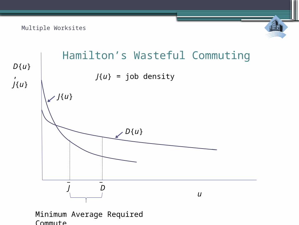
Hamilton (JPE, 1982) proposed testing urban models by comparing the average job location (distance from CBD) and the average residential location.
He said this was the amount of commuting predicted by an urban model.
He found that actual commuting is 10 times this predicted commuting, so much of it is “wasteful”—and urban models are a poor guide to commuting.
Multiple Worksites
Hamilton’s Wasteful CommutingD{u},J{u}
J{u}
u
_J
D{u}
_D
Minimum Average Required Commute
J{u} = job density
Multiple Worksites
▫What Hamilton Missed
White’s Handbook chapter reviews the subsequent debate. Hamilton did not consider
Non-central employment
Non-radial streets
Multiple-worker households
Multiple Worksites
▫Post-Hamilton Studies of Wasteful Commuting
White (JPE, 1988) uses data on actual job and housing locations, commuting distance between zones (e.g. zip codes), and linear programming to make all job or housing trades that would lower commuting costs—the spirit of an urban model.
She finds that actual commuting is only 10% greater than predicted—not 10 times as in Hamilton.
As she recognizes, she does not consider within-zip-code commuting.
Multiple Worksites
▫Post-Hamilton Studies of Wasteful Commuting, 2
Kim (JUE, 1995) has data for 1,500 zones in LA.
He can identify 1- and 2-worker households.
His linear program also finds trades that cut commuting distance, but 2-worker households can only trade jobs, not houses (so partners are not separated).
He finds that actual commuting is 50 percent above predicted for 1-worker households and 26 percent above predicted for 2-worker households.
Multiple Worksites
▫Post-Hamilton Studies of Wasteful Commuting, 2
Work still to do:
Add other benefits from job or housing location.
Introduce optimal job location.
Improve measures of commuting costs (e.g. by introducing congestion).