Efficient Collision Detection for Spherical Blend Skinning

Ladislav Kavan∗CTU in Prague / Trinity College Dublin

Carol O’SullivanTrinity College Dublin

Jirı ZaraCTU in Prague

(a) (b) (c) (d)

Figure 1: (a) shoulder twist deformed by linear blend skinning produces the candy-wrapper artifact, (b) bounding spheres for linear blendskinning refitted by [Kavan and Zara 2005a], (c) the same posture deformed by spherical blend skinning [Kavan and Zara 2005b], (d)bounding spheres for spherical blend skinning refitted using the algorithm introduced in this paper. Efficient refitting of bounding spheres isa crucial component of our fast collision detection algorithm.

Abstract

Recently, two algorithms improving the real-time simulation of ar-ticulated models in virtual environments have been published: 1)fast collision detection for linear blend skinning and 2) sphericalblend skinning. Both linear and spherical blending solve the skin-ning problem of a skeletally controlled 3D model (e.g., an avatar),but only spherical blending avoids artifacts such as the candy-wrapper. However, to date, fast collision detection has been limitedto linear blending. This paper describes how to perform collisiondetection for models skinned with the more sophisticated sphericalmethod. As a result, both high-quality skinning and fast and exactcollision detection can be achieved – there is no longer any needfor a trade-off. The generalization from linear to spherical blendinginvolves the construction of rotation bounds, derived using a quater-nion representation. The resulting algorithm is simple to implementand fast enough for real-time virtual reality applications.

CR Categories: I.3.7 [Computer Graphics]: Three-DimensionalGraphics and Realism—Animation

Keywords: collision detection, on-demand refitting, sphere refit-ting, SBS, spherical blending

1 Introduction

Collision detection (CD) is a challenging problem, mainly becauseof its high computational complexity for typical models. Collisionqueries are necessary in order to resolve interactions between a vir-tual character and its environment, as well as among several virtualcharacters themselves. Since a fast response time is essential forreal-time virtual reality applications, most current systems perform

∗e-mail: kavanl1@fel.cvut.cz

CD only with a considerably simplified geometry (e.g., a charac-ter replaced by an articulated structure of boxes). This, of course,provides only a rough estimate of actual collisions, making someartifacts visible (such as interpenetration or bouncing before con-tact). In many situations a precise (mesh-exact) CD is much moredesirable, and in certain cases is unavoidable, e.g., in medical ap-plications or virtual prototyping.

Recently, a CD algorithm has been developed, which offers exactand fast CD for 3D models deformed by linear blend skinning [Ka-van and Zara 2005a]. Unfortunately, linear blend skinning (alsoknown as skeleton subspace deformation, vertex blending or en-veloping) is infamous for its failures, such as the candy-wrapper(shoulder-twist) artifact, see Figure 1(a). This problem can besolved by spherical blend skinning [Kavan and Zara 2005b]: an al-gorithm not only useful for deforming virtual creatures and avatars,but also for cloth and other objects. Spherical blending works byblending rotations (represented by quaternions) instead of blendingvertex positions as in linear blend skinning. The result of sphericalblending applied to the same data can be seen in Figure 1(c).

In a practical application, however, we need both high-quality skin-ning and fast CD simultaneously. Unfortunately, the previous CDalgorithm for skeletally deformable objects substantially exploitsthe linearity of linear blending. Specifically, it relies on the fact thatlinear blending interpolates always within the convex hull of the in-put vertices. Since this condition is not true in spherical blending,it is not possible to use the previous collision detection algorithm –bounding spheres constructed by the previous algorithm no longerenclose the skin. This is because spherical blending does not col-lapse the skin during deformation, as does linear blending.

In this paper we show that, using bounds on the unit quaternionsphere, it is possible to achieve fast CD also for spherical blend-ing. Although it is of course a little more difficult than in the linearcase, the resulting algorithm is almost as easy to implement and thecomputational complexity of the presented algorithm is almost thesame as that of the linear version.

The proposed CD algorithm is based on a bounding-volume hierar-chy (BVH). This concept has been proven to be very efficient forboth rigid and deformable objects, even though it has its limitations,e.g., efficient self-collision detection requires additional treatment[Volino and Magnenat Thalmann 1995]. Concerning deformableobjects, it is essential to find a way to refit the bounding volumes

when the object deforms. It has been shown recently [Larsson andAkenine-Moller 2003; James and Pai 2004; Kavan and Zara 2005a]that one of the most efficient approaches is on-demand (lazy) re-fitting, which refits the spheres only when they are required by theCD algorithm. Actually, the main difference between the above-mentioned methods is in the refitting operation. The reason is thatthe refitting operation must exploit the properties of the specific de-formation model, so that it can work efficiently.

The main contribution of this paper is a procedure for refitting ofbounding spheres for spherical blend skinning with sublinear timecomplexity (with respect to the number of vertices). This refittingoperation is actually an extension of the previous refitting for linearblending, because spherical blending decomposes to a linear androtational component. However, the resulting algorithm is almostas fast as in the case of linear blending, and thus provides a way ofexact and efficient CD for 3D models deformed by spherical blend-ing.

2 Related Work

For a survey of CD methods, see [Ericson 2004; Jimenez et al.2001]. Teschner et al. present a survey specialized on deformableCD [2004]. In this paper, we focus on CD algorithms basedon a BVH. Common bounding volumes are: spheres [Quinlan1994; Guibas et al. 2002], AABBs [van den Bergen 1997], k-DOPs [Klosowski et al. 1998], and OBBs [Gottschalk et al. 1996].Other interesting BVH are QuOSPO-trees [He 1999], BoxTrees[Zachmann 2002] and sphere-swept BVHs [Larsen et al. 1999].

A restriction of most CD algorithms (including ours) is that theyconsider collisions only at discrete time intervals. It means thatsome collisions may be missed, especially for small, fast movingobjects. This shortcoming has been addressed by proposing so-called continuous CD algorithms. Based on a simplified motionmodel, they find a first time of contact for a given period of time[Redon et al. 2002]. Continuous CD algorithms have been proposedalso for articulated models [Redon et al. 2004], but only articulatedobjects composed of rigid parts were considered (such as robots).

In this paper, we focus on spherical blend skinning and exact CDalgorithms based on a BVH, specifically hierarchies of boundingspheres. Spheres were first used for rigid body CD in [Quinlan1994]. The extension of BVH-based CD for deformable objectswas presented first for AABBs by van den Bergen [1997] and laterimproved by Larsson and Akenine-Moller [2001]. The basic ideaof those algorithms is to refit all the bounding volumes during abottom-up traversal of the tree. A similar algorithm for spheres ispresented in [Brown et al. 2001]. Bottom-up refitting is consid-erably faster than rebuilding the complete BVH, but it obviouslywastes time, because not all bounding volumes are necessary forsubsequent CD query.

Much more efficient is an on-demand refitting, which recom-putes bounding volumes only when required by the CD algorithm.This was first applied for k-DOPs and linear morphing by Lars-son and Akenine-Moller [2003] and improved later by Klug andAlexa [2004]. The on-demand refitting procedure must be very fastto evaluate – it cannot work by considering the actual vertex dis-placements (which would be slower than the bottom-up refitting).The refitting should work in time sublinear with respect to the num-ber of vertices, which can only be done by exploiting the propertiesof the actual deformation model. This is also the main drawbackof this approach: it does not work for general deformations – eachdeformation model needs a special refitting procedure. Such refit-ting of spheres is presented in [James and Pai 2004] for reduced

deformation model and in [Kavan and Zara 2005a] for linear blendskinning. Another collision detection method specialized for skele-tally deformable 3D models can be found in [Heim et al. 2004], buttheir refitting procedure is limited only to a single layer of boundingvolumes (no hierarchy), which is restrictive especially for detailed3D models.

Even though specialized refitting operations ensure very efficientCD, alternative CD algorithms have also been proposed for de-formable models, which are not based on a BVH. Instead, theymake use of spatial hashing [Teschner et al. 2003], image-spacetechniques [Heidelberger et al. 2004; Govindaraju et al. 2003], orchromatic decomposition [Govindaraju et al. 2005]. The big advan-tage of these methods is their generality, i.e., they do not depend onany specific deformation model. Sometimes this is necessary, forexample when the deformations are computed during a complexrun-time simulation. On the other hand, making no assumptionsabout the deformation model restricts the time complexity to be atleast linear, i.e., disables sublinear time complexity. The reason isobvious: if we allow arbitrary deformations, we must check the dis-placements of all vertices at runtime. This is especially painful ifthe deformations are computed on another processor. Therefore, wefind it advantageous to apply on-demand refitting whenever possi-ble, not only because of the sublinear execution time, but also be-cause it allows CD to be executed in parallel with the computationof vertex displacements (typically done on a GPU).

As an alternative to spherical blending, it would be possible to con-sider a different skinning method which does not produce artifacts.For example, [Mohr and Gleicher 2003] reduce the artifacts of lin-ear blending by adding auxiliary joints and recomputing the vertexweights using examples. Even though in this case we could ap-ply the CD solution for linear blending [Kavan and Zara 2005a],there would be associated drawbacks. First, the runtime complex-ity of Kavan and Zara’s algorithm depends on the number of joints,thus addition of auxiliary joints increases the time complexity. Infact, the more joints we add, the better approximation of sphericalblending we obtain. Second, Mohr and Gleicher’s approach [2003]requires example skins, whose production can be costly. Sphericalblend skinning, on the other hand, uses the same input data as linearblending – no extra work is necessary.

A skinning similar to spherical blending is described by [Hejl2004]. This is actually a simpler algorithm which works correctlyonly if vertices are influenced solely by neighbouring bones, i.e.,bones that share a common joint, an assumption that is only validfor some 3D models. The collision detection method described inthis paper can be directly applied for Hejl’s skinning (no modifica-tions are necessary as spherical blending is more general).

Other advanced skinning techniques have been proposed recently,allowing realistic simulation of muscle bulges and other effects.Even though delivering high-quality skin deformations, they areusually much more complicated (and slower) than linear or spheri-cal blend skinning. The existence of efficient sphere refitting oper-ation for such deformation models is therefore questionable.

Our Contribution: In this paper, we present a novel CD algorithmespecially designed for spherical blend skinning. At its core is anefficient sphere refitting operation, similar in spirit to Kavan andZara’s [2005a]. However, since spherical blending works with ro-tations, the generalization from this previous linear algorithm is nottrivial. This is achieved by the construction of bounds on the unitquaternion sphere. Despite the fact that the derivation and justi-fication of the sphere refitting is not straightforward, the resultingalgorithm is simple to implement and fast to execute. We demon-strate this on several practical examples of character animation.

Conventions: We denote the d-dimensional Euclidean space as Rd

and we write its elements (vectors) in bold. The zero vector is de-noted as 0. The vector v ∈ Rd consists of components (v1, ...,vd)T .In order to simplify notation, we introduce the set of all possibleconvex weights:

Wd = {x ∈ Rd : x1 ≥ 0, . . . ,xd ≥ 0,d

∑i=1

xi = 1}

The convex hull of set A ⊆ Rd , i.e., the smallest convex set con-taining A, is denoted as CH(A). We denote the dot product of twovectors v1 ∈ Rd ,v2 ∈ Rd as (v1,v2) and the norm ‖v1‖ as a shortcutfor√

(v1,v1). The 3-dimensional sphere surface of unit quater-nions is denoted as S3 = {x ∈ R4 : ‖x‖ = 1} (note that we identifyquaternions with R4 vectors).

3 Skinning and Collision Detection

This section recapitulates the spherical blend skinning algorithmand the basics of collision detection based on a BVH, as describedin [Kavan and Zara 2005b; Kavan and Zara 2005a]. The input ofboth linear and spherical blend skinning consists of a skin, a skele-ton, and vertex weights for each vertex-joint pair. The skin is just a3D triangular mesh and the skeleton is a rooted tree. The nodes ofthis tree represent joints and the edges can be interpreted as bones.The vertex weights describe the amount of influence of individualjoints on the position of the vertex in the deformed skin. Note thatthe input for linear blend skinning is the same, i.e., identical inputfiles are used for both linear and spherical skinning.

Let us assume that the joints are stored in an array, with every jointreferenced by an integer number, starting from zero. In the refer-ence posture, each joint has an associated local coordinate system.During animation, the joints rotate – we do not consider translationor scale. The transformation from the reference coordinate systemof joint j to its coordinate system in the animated posture can beexpressed as a rigid transformation matrix. We can compute thismatrix as a multiplication of successive joint transformations. Wedenote this matrix as Cj (like the “complete” transformation ma-trix).

We assume that vertex v is attached to joints j1, . . . , jn with weightsw = (w1, . . . ,wn) (The indices j1, . . . , jn are integers referring tojoints that influence a given vertex – they can be interpreted as in-dices into the array of joints.) In order to have properly definedblending, the weights must be convex: w ∈ Wn. The set of joints{ j1, . . . , jn} is called the joint-set influencing the vertex v and is de-noted as J(v). The i-th component of vector w, wi, represents theamount of influence of joint ji.

Let us denote the unit quaternions corresponding to the rotationparts of matrices Cj1 , . . . ,Cjn as q1, . . . ,qn (the conversion proce-dure can be found in [Eberly 2001]). During skin deformation,quaternions are blended using the QLERP method (Quaternion Lin-ear Interpolation), computing w1q1+...+wnqn

‖w1q1+...+wnqn‖ and converting the re-sult to a rotation matrix Qw. The vertex position in the deformedmesh is then computed as:

v′ = Qw(v−rc)+n

∑i=1

wiCji rc (1)

where rc is the rotation center, defined as the point whose trans-formations by matrices Cj1 , . . . ,Cjn are as close as possible. For thepurpose of on-demand refitting, it is sufficient to take the rc as com-puted by spherical blending; for details please see [Kavan and Zara2005b].

The interpretation of the spherical blending Equation (1) is as fol-lows: we call the first term Qw(v− rc) the spherical part and thesecond one ∑n

i=1 wiCji rc the linear part. The linear part is actu-ally nothing but a linear blending applied to the rotation center rc.This part becomes important if the set of influencing bones is notsimple, i.e., if it contains more than two non-neighbouring joints.In this case the translation between the joints must be interpolated,which is exactly the role of the linear part of Equation (1). Thespherical part, on the other hand, interpolates rotation of the in-fluencing joints. The linear quaternion blending (QLERP) used toproduce Qw is the reason why spherical blend skinning does not ex-hibit artifacts (which would appear if we blended matrices insteadof quaternions, just like in linear blend skinning). More details canbe found in [Kavan and Zara 2005b].

For on-demand refitting, it is important that the final vertexposition v′ will no longer lie in CH(Cj1 v, . . . ,Cjn v), whichwas true for linear blending (and subsequently exploited in thesphere refitting for linear blend skinning). In spherical blend-ing, v′ lies instead on a helical surface A, given as A ={

Qw(v−rc)+∑ni=1 wiCji rc : w ∈Wn

}. In simple situations, the set

A becomes a spherical arc or surface. The main problem of the on-demand refitting for spherical blending is to find an efficient boundfor a subset of set A. This is obviously not as simple as in the caseof linear blending, and none of the previous refitting methods canbe applied for this task.

For our collision detection algorithm we need a tree of boundingspheres. We build this tree for the reference position of the 3Dmodel, using the same algorithm as in [Kavan and Zara 2005a], thusenabling a fair comparison of the results. The sphere tree is builtby a top-bottom algorithm, which starts by first bounding the whole3D model within one sphere. In the next steps, we split the geom-etry into two parts and proceed recursively, computing the minimalenclosing sphere with Gaertner’s algorithm [1999]. When the com-plete binary tree is constructed, some nodes are pruned using thesame heuristics as in [Kavan and Zara 2005a]. Generally, we prunea node if its bounding sphere has a similar size to the boundingsphere of the parent node, thus discarding less useful nodes andobtaining a general order tree instead of a binary one.

For the actual collision detection, we apply the standard algorithmbased on a BVH. As input we have two 3D models, each equippedwith a BVH. The task is to either find all colliding triangles, or findat least one (if any). The algorithm proceeds as follows: first, wetest the root spheres for intersection. If disjoint, we end up with nocollisions. If intersecting, we move to the next level in one of thehierarchies and continue recursively. In the final level we performintersection tests on individual triangles. The only modification wemake to this standard algorithm is the sphere refitting, which is in-serted just before the intersection test. In this way we ensure thatwe work with correct bounding spheres, even though the 3D modelhas been deformed.

4 Efficient Refitting of Spheres

The crucial part of a BVH-based CD algorithm for deformable ob-jects is the refitting operation. As mentioned in the introduction,the refitting procedure must work in an on-demand way, so that itcan be executed on spheres in any order. Moreover, the refittingalgorithm must be sublinear with respect to the number of vertices.To achieve this, we exploit the fact that the animation is only con-trolled by the joint transformation matrices Cj (all other data areconstant). It is therefore possible to base the refitting proceduresolely on some precomputed information and on the actual jointtransformations. This is of course much more efficient than driving

the refitting by vertex displacements, because the number of jointsis usually orders of magnitude smaller than the number of vertices.

4.1 Problem Decomposition

We assume that the skin of the input 3D model consists of triangles.Since triangles and bounding spheres are always convex, it is suffi-cient to enclose only the vertices of a triangle in order to bound thewhole triangle. During sphere tree construction, we ensure that thebounding spheres in the children nodes enclose the same geometryas the bounding sphere in the parent node. Moreover, we requirethat each triangle is bounded by a single sphere (it is not sufficientthat a triangle is covered only by a union of spheres). Let us assumethat we are refitting a sphere S with center p and radius r, which en-closes some set of triangles. We denote all vertices of those trian-gles as v1, . . . ,vt . For simplicity of notation, we first assume that allthese vertices are influenced by the same joint-set J = { j1, . . . , jn},that is J = J(v1) = . . .J(vt ). The task is to compute a new spherewhich will enclose vertices v′1, . . . ,v

′t , computed by Equation (1).

The trick to obtaining an algorithm sublinear in t is to replace theset of vertices {v1, . . .vt} by the bounding sphere S, which is correctbecause {v1, . . . ,vt} ⊆ S. That is, instead of bounding v′1, . . . ,v

′t we

could bound the set

⋃w∈Wn

(Qw(S−rc)+

n

∑i=1

wiCji rc

)(2)

Considering the whole sphere S of points instead of only one pointis not a big problem, as shown in Section 4.3. A more seriousproblem is that the set (2) is very conservative, because it disre-gards the actual vertex weights of v1, . . .vt . This means that (2)actually bounds all skin deformations that could be ever producedby spherical blending for the given posture. Obviously, this wouldproduce a very loose bounding sphere, useless for collision detec-tion. It is therefore necessary to take the actual vertex weights intoaccount. This is done by computing low and high bounds of thevertex weights for all joints in our joint-set J. For every joint j ∈ Jwe denote the weight bound as 〈l j,h j〉, making sure that the weightof each vertex v1, . . .vt with respect to joint j is within this interval.Using the weight bounds li and hi, we define the set W ′

n of limitedconvex combinations:

W ′n = {w ∈ Rn : li ≤ wi ≤ hi, i = 1, . . .n,

n

∑i=1

wi = 1}

and apply this set in (2) instead of Wn. The final set to be boundedby the refitted sphere is therefore

⋃w∈W ′

n

(Qw(S−rc)+

n

∑i=1

wiCji rc

)(3)

The set W ′n has a nice geometric interpretation: it is the intersection

of an n-dimensional box {w ∈ Rn : li ≤ wi ≤ hi, i = 1, . . .n} with ahyperplane {w ∈ Rn : ∑n

i=1 wi = 1}. It means that W ′n is a bounded

convex set in Rn and can therefore be expressed as a convex hullof m points (because of the equivalency of bounded H-polytopesand V-polytopes [Matousek 2002]). We denote these m points asc1, . . . ,cm and call them corners (where m is the number of verticesof the corresponding V-polytope). The corners depend only on ver-tex weights, which means that they can be precomputed during thesphere tree construction. The expression of set W ′

n exploiting cor-ners is as follows:

W ′n = CH(c1, . . . ,cm) =

{m

∑k=1

ukck : u ∈Wm

}(4)

We derive the bound of set (3) in three steps. In the first step,we bound the linear component ∑n

i=1 wiCji rc (Section 4.2) and inthe second step, we bound the spherical part Qw(S − rc) (Sec-tion 4.3). Finally, both of these bounds are simply added together(Section 4.4) to create the resulting refitted sphere. The resultingalgorithm is presented in Section 4.5. If the reader is not inter-ested in the derivation and justification of our approach, he or sheis encouraged to skip the following sections and proceed directly toSection 4.5. Even though the material in Sections 4.2, 4.3, and 4.4is essential to show the validity of our algorithm, it is not necessaryfor a practical implementation.

4.2 Bounding the Linear Part

Unlike the bound of the spherical part, the bound of the linear partof set (3) can be done in a way similar to [Kavan and Zara 2005a](the situation is actually more simple here, because we are boundingpoints instead of spheres as in the previous article). This is becausethe linear part is actually nothing but a linear blending applied to therotation center rc, which is a point computed by the spherical blendskinning algorithm for a given skeleton posture: it is independentof the vertex weights.

Thanks to the expression of W ′n using corners (Equation (4)), we

can rewrite the linear part of set (3) as{n

∑i=1

wiCji rc : w ∈W ′n

}=

{n

∑i=1

(m

∑k=1

ukcki

)Cji rc : u ∈Wm

}

where cki denotes i-th component of vector ck. In the latter term,we can swap the sums, because

n

∑i=1

(m

∑k=1

ukcki

)Cji rc =

m

∑k=1

uk

(n

∑i=1

ckiCji rc

)

We denote the transformations of the rotation center as:

r′k =n

∑i=1

ckiCji rc, k = 1, . . . ,m (5)

which is correct because ck ∈ W ′n and thus ∑n

i=1 cki = 1. Equa-tion (5) is actually nothing but linear blending applied to rc withweight vector ck. If we put the equations together, we can write theresulting bound of the linear part as{

n

∑i=1

wiCji rc : w ∈W ′n

}=

{m

∑k=1

ukr′k : u ∈Wm

}= CH(r′1, . . . ,r

′m)

To conclude: the bound of the linear part is just a convex hull of sev-eral 3D points. These points are given by the precomputed cornersand Equation (5). Please note that, although we use the concept ofthe convex hull in our derivation, the convex hull is actually nevercomputed in our algorithm (bounding spheres are used instead, seeSection 4.5).

4.3 Bounding the Spherical Part

Bounding the spherical part of set (3) is a little bit more tricky,because we must deal with the linear quaternion interpolation(QLERP) hidden in Qw. Recall that we are refitting sphere S withcenter p and radius r, expressed in the reference position. First, wereplace the sphere S by its center p:⋃w∈W ′

n

Qw(S−rc) ={

Qw(p−rc) : w ∈W ′n}⊕{x ∈ R3 : ‖x‖ ≤ r

}

where r is the radius of sphere S and ⊕ denotes the Minkowski sum.However, the Minkowski sum in the previous equation is actuallynothing but a convolution of set {Qw(p−rc) : w ∈W ′

n} with a zerocenter sphere of radius r. In the following, we derive the boundingsphere of {Qw(p−rc) : w ∈W ′

n}. At the end, we account for theMinkowski sum (convolution) by simply increasing the radius ofthe resulting sphere by r (line 16 of Algorithm 1). The rest of thissection is organized as follows: first, we compute bound on the setof rotations Qw and express it as a subset of unit quaternion sphereS3. Second, we apply all rotations from this set to rotate the vectorp− rc. The result is some subset of R3, which is enclosed by afinal bounding sphere of the spherical part. The reader should notget confused by the fact that the bounds in both steps will have thesame shape (a spherical cap, defined below). The difference is thatthe bounding of rotations occurs in R4, whereas the bounding ofrotated vectors takes place in R3.

Recall that we denoted the quaternions corresponding to the rota-tional parts of matrices Cj1 , . . . ,Cjn by q1, . . . ,qn. Then Qw is arotation matrix given by the quaternion w1q1 + . . . + wnqn. Thisis correct, because every non-zero quaternion determines a unique3D rotation (even though not vice-versa). We proceed by con-structing a bound of all rotations given by the set of quaternions{w1q1 + . . .+wnqn : w ∈W ′

n}. We exploit the fact that QLERP ap-plies linear combinations of quaternions, and that quaternions canbe interpreted as R4 vectors. The first step will be therefore similarto that described in Section 4.2, just in R4 instead of R3. Using thesame corners c1, . . . ,cm as in Section 4.2, we compute another setof quaternions q′

1, . . . ,q′m given by

q′k =

n

∑i=1

ckiqi, k = 1, . . . ,m

which satisfy the property{w1q1 + . . .+wnqn : w ∈W ′

n}

={

u1q′1 + . . .+umq′

m : u ∈Wm}

This can also be proven by swapping sums as in Section 4.2. It istherefore sufficient to construct a bound for rotations correspondingto quaternions from CH(q′

1, . . . ,q′m).

Unfortunately, this cannot be done simply by a convex boundingvolume, as in Section 4.2, because in this case, we are workingin a non-linear space (spherical surface). Linear bounds, such asconvex hull, obviously cannot work in curved spaces. For example,it is not correct to just rotate vector p−rc by quaternions q′

1, . . . ,q′m

and bound the results by a 3D enclosing sphere. In order to obtaina valid bounding volume, we have to appropriately bound the set ofrotations given by CH(q′

1, . . . ,q′m).

We have chosen only a simple bound of rotation sets: a sphericalcap on S3 (the sphere of all unit quaternions). Generally, we definea cap in any dimension as a non-empty intersection of a spheresurface with a halfspace. In the following, we will also need anotherdefinition of cap, given by the center cs of the sphere, point as onthe sphere’s surface (the cap’s apex) and an angle αs ∈ 〈0,π〉. Ifwe denote the radius of the sphere as rs = ‖as − cs‖, then the capaccording to the second definition is expressed as{

x ∈ Rd : ‖x−cs‖ = rs, (x−cs,as −cs) ≥ r2s cos(αs)

}It is not difficult to prove that both definitions are equivalent, seeLemma 1 in the Appendix. An example of a cap is shown in Fig-ure 2.

The bound of a set of rotations expressed by a cap C on S3 has anice geometric interpretation. Let us denote the apex of cap C asaC and the angle as αC (in this case, the center cC = 0 and radius

�scs

as

halfspace

sphere

cap

Figure 2: Example of a cap in R2 with center cs, apex as and angleαs. In this case the cap is just a spherical arc.

rC = 1, because S3 is a zero centered sphere with unit radius). Sincewe are considering S3, the apex aC is a unit quaternion representingsome rotation RC. Then all rotations represented by cap C can beobtained by composing RC with a rotation about an arbitrary axisand angle within 〈0,2αC〉 (2αC because quaternions work with halfof the angle of rotation, see for example [Eberly 2001]). If we havethe set of rotations bound by cap C ⊆ S3, we can bound our originalset {Qw(p−rc) : w ∈W ′

n} by ρ = {R(p−rc) : R ∈C}, where C isinterpreted as a set of rotations. But the set ρ is nothing but the setof all possible rotations of vector RC(p−rc) along an arbitrary axisand angle within 〈0,2αC〉. It means that ρ is nothing but anotherspherical cap (but now in R3)! The apex of cap ρ is RC(p− rc),center is 0 and angle 2αC .

Since we are constructing a cap on S3, we normalize our quater-nions q′

1, . . . ,q′m to unit quaternions: q′′

k = q′k/‖q′

k‖, k = 1, . . . ,m.We can work with q′′

k instead of q′k, because Lemma 2 from

the Appendix shows that the sets of rotations corresponding toCH(q′

1, . . . ,q′m) and CH(q′′

1, . . . ,q′′m) are the same. What remains

is to construct a cap on S3 containing our quaternions q′′1 , . . . ,q′′

m.

In order to construct this cap, we bound q′′1 , . . . ,q′′

m by an enclosingsphere E ⊆ R4 with center cE and radius rE . It would be possibleto use again the randomized algorithm [Gaertner 1999] which findsthe smallest enclosing sphere, but we found that just an approxi-mate enclosing sphere performs better. The approximate enclosingsphere is computed in the same way as in [James and Pai 2004] (butin R4 in our case), i.e., by taking the average of q′′

1 , . . . ,q′′m as the

center and then determining the smallest possible radius which stillgives a correct enclosing sphere.

After computing the enclosing sphere E we are almost done, be-cause E ∩ S3 is the desired cap. This is illustrated in Figure 3 andverified in Lemma 3 and Lemma 4 in the Appendix. We can assumethat the radius of sphere E satisfies rE < 1: if not, we can simplyconsider the whole S3 (of radius 1) which bounds all rotations, asthe bounding cap (although it should be noted that this situationnever occurred during practical experiments).

Now it is straightforward to derive the resulting cap C′ ⊆ R3 suchthat {Qw(p−rc) : w ∈W ′

n} ⊆ C′. We denote by Qc the rotationcorresponding to cE . The apex of the cap C′ is then Qc(p−rc), thecenter is 0 and the angle is

α = 2arccos(dH), dH =1+‖cE‖2 − r2

E

2‖cE‖ (6)

where dH denotes the distance from H to 0, as computed inLemma 3 and illustrated in Figure 3. Note that, since the sphereE intersects S3, it cannot happen that E is strictly inside S3, i.e.,‖cE‖ + rE < 1 cannot be true. Therefore, ‖cE‖ + rE ≥ 1, thus

S3

E

q''1

q''m

H

���

0

cE

dH

Figure 3: To construct the bounding cap (in this picture just thespherical arc) for quaternions q′′

1 , . . . ,q′′m, we first create an enclos-

ing sphere E (not necessarily the smallest one). The cap is thengiven as E ∩ S3, which can be equally expressed as H ∩ S3, whereH is a halfspace from Lemma 3. A formula for distance dH from Hto 0 is also derived in Lemma 3. The distance dH is used to computethe angle α .

−r2E ≤−(1−‖cE‖)2 = −1+2‖cE‖−‖cE‖2 from which follows:

dH ≤ 1+‖cE‖2 −1+2‖cE‖−‖cE‖2

2‖cE‖ =2‖cE‖2‖cE‖ = 1

Since obviously 0 ≤ dH , the arccos in Equation 6 is well definedand α ∈ 〈0,π〉.The resulting sphere returned for the bound of the spherical partis nothing but a minimal enclosing sphere of cap C′. We denotethis minimal enclosing sphere as F ⊆ R3 and we compute it easily:its center is cos(α)Qc(p− rc) and radius is sin(α)‖Qc(p− rc)‖ =sin(α)‖p− rc‖, where α is given by Equation 6. This is proven inLemma 5 and illustrated in Figure 4.

�

Q ( - )c cp rcap C'

bounding sphere

0

Figure 4: If the cap C′ centered in the origin has apex Qc(p −rc) and angle α , then its minimal enclosing sphere has centercos(α)Qc(p−rc) and radius sin(α)‖p−rc‖.

4.4 Putting the Bounds Together

To construct the final bounding sphere of set (3), it remains just tocombine the bound of the linear part and the bound of the sphericalpart. Recall that, in Section 4.2, the bound of the linear part wasexpressed as CH(r′1, . . . ,r

′m) and, in Section 4.3, the spherical part

was bound by sphere F . The bound of both parts can therefore beexpressed as CH(r′1⊕F, . . . ,r′m ⊕F), i.e., the final bounding sphereencloses r′1 ⊕F, . . . ,r′m ⊕F . This enclosing sphere is again com-puted only by a simple approximation (the same as before): thecenter of the enclosing sphere is set to the average of the centersof r′1 ⊕F, . . . ,r′m ⊕F , and the smallest possible radius is computedin a straightforward way. Note that this enclosing sphere is not thesmallest possible enclosing sphere. However, as suggested alreadyby [James and Pai 2004; Kavan and Zara 2005a], it is more efficient

for collision detection than computation of the minimal enclosingsphere. The correctness of collision detection is of course not af-fected by employing bigger-than-necessary spheres.

In the beginning of Section 4, we assumed that all vertices v1, . . . ,vtof the reference sphere S are assigned to only one joint-set J. If thisis not the case, i.e., the vertices v1, . . . ,vt are influenced by morejoint-sets J1, . . . ,Jz, we simply repeat the same algorithm for each ofthese joint-sets. This way, we obtain spheres r′1,1 ⊕F1, . . . ,r′m1,1

⊕F1,r′1,2 ⊕F2, . . . ,r′m2,2

⊕F2, . . . ,r′1,z ⊕Fz, . . . ,r′mz,z ⊕Fz and enclosethem by one bounding sphere as before.

4.5 Final Algorithm

This section presents the final sphere refitting algorithm. For sim-plicity, we write [c,r] to denote a data structure describing a spherewith center c and radius r. The symbol cki on lines (7) and (8) de-notes the i-th component of an n-dimensional vector ck. In list L2are actually stored points q′′

k , but for convenience, we treat them asspheres with zero radius: [q′′

l ,0].

Algorithm 1: Sphere Refitting for Spherical BlendingInput: S = [p,r] – sphere to be refitted

C1, . . . ,CN – joint transformation matricesJ – list of joint-sets influencing sphere Sc1, . . . ,cm – corners describing the bound of weightsrc – rotation center

Output: sphere S refitted for current skin deformationSPHEREREFIT(S)(1) L1 = empty list(2) for k = 1 to m(3) qi = MATRIX2QUAT(Ci)(4) foreach joint-set { j1, . . . , jn} ∈ J(5) L2 = empty list(6) for k = 1 to m(7) r′k = ∑n

i=1 ckiCji rc

(8) q′k = ∑n

i=1 ckiqi

(9) q′′k = q′

k/‖q′k‖

(10) insert sphere [q′′l ,0] into list L2

(11) [cE ,rE ] = BOUNDINGSPHERE(L2)(12) Qc = QUAT2MATRIX(cE/‖cE‖)

(13) α = 2arccos( 1+‖cE‖2−r2E

2‖cE‖ )(14) for k = 1 to m(15) insert sphere [r′k + cos(α)Qc(p− rc),sin(α)‖p−

rc‖] into list L1(16) return BOUNDINGSPHERE(L1) + [0,r]

The addition of [0,r] on line (16) simply inflates the radius ofthe resulting sphere by r. The sphere refitting algorithm usesthree subroutines: MATRIX2QUAT, QUAT2MATRIX, and BOUND-INGSPHERE. The first two convert between quaternion and ma-trix representation (note that this would not be necessary if our ap-plication worked internally with quaternions instead of matrices).These routines are usually a standard part of mathematical libraries[Eberly 2001]. Concerning BOUNDINGSPHERE, we use only thesimple approximate algorithm for the bounding sphere of spheresmentioned before: setting center as the average of centers of in-put spheres and computing the minimal possible radius straigtfor-wardly.

Level Reference Linear Blending Spherical Blending Optimal1 34.55 34.55 34.55 72.17 72.17 72.17 79.55 79.55 79.55 34.41 34.41 34.412 18.11 18.86 19.74 26.17 31.58 34.48 26.23 33.95 37.84 17.97 22.05 26.573 3.11 7.38 10.47 3.11 8.40 14.89 3.11 8.89 17.33 3.11 7.39 10.134 0.98 3.68 6.23 0.98 4.03 7.96 0.98 4.12 9.23 0.98 3.69 6.475 0.24 1.69 3.69 0.24 1.80 5.05 0.24 1.83 5.28 0.24 1.70 4.336 0.20 0.91 2.84 0.20 0.97 3.50 0.20 0.98 4.01 0.20 0.92 2.897 0.15 0.61 2.09 0.15 0.65 2.68 0.15 0.66 3.58 0.15 0.61 2.098 0.15 0.42 1.16 0.15 0.43 1.59 0.15 0.43 1.71 0.15 0.42 1.299 0.12 0.30 0.54 0.12 0.30 0.59 0.12 0.30 0.78 0.12 0.30 0.54

Table 1: This table lists minimal, average and maximal radii of a spheres in the creature model’s sphere tree. Reference: spheres for thereference posture (Figure 5 top). Linear Blending: animated posture in Figure 5 middle, skin deformed by linear blending, spheres refittedby Kavan and Zara’s algorithm [2005a]. Spherical Blending: animated posture in Figure 5 bottom, skin deformed by spherical blending,spheres refitted by Algorithm 1. Best: animated posture in Figure 5 bottom, skin deformed by spherical blending, spheres refitted by an exactminimal enclosing sphere algorithm [Gaertner 1999].

5 Results

In order to provide comparative measurements, we execute the testson models from [Kavan and Zara 2005a]: the man model with 4435vertices, 8270 triangles and 27 joints, and the creature model with6682 vertices, 13590 triangles and 56 joints. The sphere tree is alsoconstructed in the same way. First, we investigate the tightness ofthe refitted spheres, see Figure 5 and Table 1.

Figure 5: Bounding spheres on levels 4 and 6 of the tree: Top: ref-erence posture, minimal enclosing spheres. Middle: animated pos-ture deformed with linear blend skinning (note the candy-wrapperartifact in the neck), spheres refitted by [Kavan and Zara 2005a].Bottom: the same posture as in the middle row deformed by spher-ical blend skinning, spheres refitted by Algorithm 1.

We observe that the size of the refitted spheres is almost the same asthe size of the spheres in the reference posture, which are optimalbecause they are computed by an exact minimal enclosing spherealgorithm [Gaertner 1999]. Also, the size of the spheres refitted forlinear and spherical blending is similar – even though the geome-

tries of the deformed skins are different (observe the candy-wrapperartifact in the middle row of Figure 5). The average radii of spheresare reported in Table 1.

We measured the speed of the collision detection and sphere refit-ting on a 2.5GHz Athlon PC under normal working conditions. Theanimations are adapted from [Kavan and Zara 2005a], except thatspherical blending is used instead of linear. Please note that thecomparison of timings of sphere refitting for linear and sphericalblending cannot be exact, because both skinning methods produceslightly different geometry (and thus possibly also a different num-ber of intersections). However, since the test animations involveonly moderate joint rotations, the difference between linear andspherical skinning is not very big (the difference is obvious onlyfor large joint rotations, e.g., the neck twist in Figure 5). The firstscenario is an animation of two walking men, shown in Figure 6.

Figure 6: One frame from the first test animation. On the right wesee spheres on levels 5 and 6 of the tree refitted by Algorithm 1.Thanks to the on-demand refitting, only 19% of spheres on the fifthlevel are refitted (9% on the sixth level).

Results for this animation are reported in the first row of Table 2.We use a new version of mathematical libraries, thus the resultsfor linear blending differ slightly from those reported in [Kavanand Zara 2005a]. We see that the slowdown caused by an ad-vanced skinning algorithm is really negligible. The refitting of all15339 spheres requires a total time of 20.15ms, which is 1.31μsper sphere. This is almost as good as sphere refitting for linearblending, which requires in average 1.21μs per sphere. In practicalsituations, of course, only a small fraction of all those spheres is re-fitted, therefore times for collision detection are much smaller, seeTable 2.

The next testing scenario is called a “worst-case scenario”, be-cause of the many colliding triangles (much more than in practicalsituations, where the collision response routines prevent such ex-treme interpenetration). In this animation, we measured besides thestandard full CD query also the average time for yes/no CD task,

Scenario LBS SBS Bottom-upMen (Full) 0.27 0.31 16.70Creatures (Full) 6.14 7.47 35.17Creatures (Yes/no) 0.72 1.44 28.67

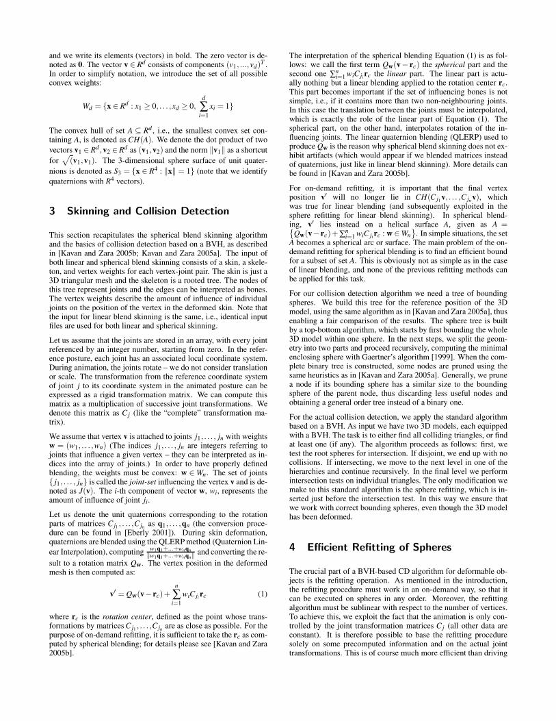
Table 2: Average times in milliseconds for one collision detectionquery in various settings. Full: CD returns set of all colliding tri-angles, Yes/no: CD returns only one pair of colliding triangles, ifany. LBS: on-demand refitting for linear blend skinning [Kavanand Zara 2005a]. SBS: on-demand refitting for spherical blendingskinning presented in this paper. Bottom-up: general bottom-uprefitting [Brown et al. 2001], applied for model deformed by spher-ical blend skinning.

which reports only whether the objects are colliding or not, withoutsearching for all colliding triangles (collision detection algorithmin this case stops when the first intersecting triangle pair is found).Measurements are reported in the second and third row of Table 2.We see that, even in difficult situations, the overhead for sphericalskinning is fortunately very low, and thus its performance is com-parable to refitting for linear blend skinning.

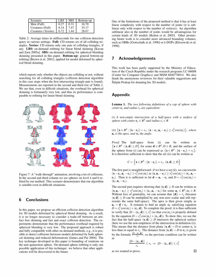
Figure 7: A ”walk-through” animation, involving a lot of collisions.In the second and third column we see spheres on level 4 and 6 re-fitted by our method. This scenario demonstrates that our algorithmis suitable even in difficult situations.

6 Conclusions

In this paper, we propose an efficient collision detection algorithmfor 3D models deformed by spherical blend skinning. As a result,it is no longer necessary to consider a trade-off between an arti-fact free skinning and fast and exact collision detection. The ex-periments demonstrate that the performance overhead required byspherical blending is very low. The proposed approach is robustand fully compatible with other on-demand methods, e.g., it is pos-sible to detect collisions between models deformed by both spheri-cal skinning and reduced deformations [James and Pai 2004]. Thekey technique developed in this paper is bounding of rotations onthe unit quaternion sphere. On-demand sphere refitting is only onepossible application of this technique: we believe that other appli-cations will be discovered in the future.

One of the limitations of the proposed method is that it has at leastlinear complexity with respect to the number of joints (it is sub-linear only with respect to the number of vertices). An algorithmsublinear also in the number of joints would be advantageous forcertain kinds of 3D models [Redon et al. 2005]. Other promis-ing future work is to consider more advanced bounding volumes,such as OBBs [Gottschalk et al. 1996] or k-DOPs [Klosowski et al.1998].

7 Acknowledgements

This work has been partly supported by the Ministry of Educa-tion of the Czech Republic under the research programs LC-06008(Center for Computer Graphics) and MSM 6840770014. We alsothank the anonymous reviewers for their valuable suggestions andStepan Prokop for donating his 3D models.

Appendix

Lemma 1. The two following definitions of a cap of sphere withcenter cs and radius rs are equivalent:

(i) A non-empty intersection of a half-space with a surface ofsphere with center cs ∈ Rd and radius rs ∈ R

(ii){

x ∈ Rd : ‖x−cs‖ = rs, (x−cs,as −cs) ≥ r2s cos(αs)

}, where

as is the apex, and αs the angle.

Proof. The half-space from (i) can be written as{x ∈ Rd : (x,d) ≥ D

}for some d ∈ Rd ,D ∈ R, and the surface of

the sphere from (i) can be expressed as{

x ∈ Rd : ‖x−cs‖ = rs}

.It is therefore sufficient to show that the set (ii) can be written as

C ={

x ∈ Rd : ‖x−cs‖ = rs, (x,d) ≥ D}

The first part is straightforward: if we have a set (ii), we can rewrite(x−cs,as −cs) ≥ r2

s cos(αs) as (x,as −cs)≥ r2s cos(αs)+(cs,as −

cs). Then it is sufficient to let d = as − cs and D = r2s cos(αs) +

(cs,as −cs).

The second part requires showing that (x,d) ≥ D can be written as(x,as − cs) ≥ r2

s cos(αs) + (cs,as − cs) for some as ∈ Rd ,αs ∈ R.Without loss of generality, we can assume that ‖d‖ = rs (because(x,d) ≥ D can be multiplied by any non-zero scalar and still rep-resents the same half-space). The apex is then given simply asas = d + cs. It remains to find an angle αs satisfying equationD = r2

s cos(αs)+(cs,d). To complete the proof, it is thus sufficientto verify that |D− (cs,d)| ≤ r2

s (so that cos(αs) is properly definedby the equation D = r2

s cos(αs)+ (cs,d)). To show this, we use thefact that the half-space (x,d) ≥ D intersects the spherical surface(here we use the non-emptiness of the intersection in definition (i)).This means that the distance from plane (x,d) = D to center cs isless than or equal to rs. The distance from (x,d) = D to cs is given

by the formula |D−(cs,d)|rs

, so the previous condition can be writtenas

|D− (cs,d)|rs

≤ rs ⇒ |D− (cs,d)| ≤ r2s

as we wanted to prove.

Lemma 2. Let q1, . . . ,qm be non-zero quaternions and n1 =q1‖q1‖ , . . . ,nm = qm

‖qm‖ the corresponding unit quaternions. Then the

set M = CH(q1, . . . ,qm) represents the same rotations as the setN = CH(n1, . . . ,nm).

Proof. We know that two non-zero quaternions p,q represent thesame rotation iff there exists k ∈ R, k �= 0 such that p = kq. First,we show that any rotation from M is also present in N. Let uschoose an arbitrary a ∈ M, i.e. a = ∑wiqi for some w ∈ Wm. We

define K = ∑wi‖qi‖ and ui = wi‖qi‖K . Obviously K > 0, ui ≥ 0 and

∑ui = 1, that is u ∈ Wm. Hence ∑uini ∈ N and to finish the firstpart of the proof it is sufficient to show that K ·∑uini = a (i.e. that∑uini represents the same rotation as a). So, we show that:

K ·∑uini = K ·∑ wi‖qi‖qi

K‖qi‖ = ∑wiqi = a

Second, we show that any rotation from N is also present in M.Let us choose an arbitrary b ∈ N, i.e. b = ∑tini for some t ∈ Wm.We define L = ∑ ti

‖qi‖ and si = ti‖qi‖L . Again, L > 0 and s ∈ Wm,

therefore ∑ siqi ∈ M. In a similar way as before we see that

L ·∑siqi = L ·∑ tiqi

‖qi‖L= ∑ tini = b

which completes the proof.

Lemma 3. Let Sa be a spherical surface in Rd with center a andradius ra. Let Sb be a sphere in Rd with center b and radius rb.Then the intersection Sa ∩Sb is a cap, i.e. Sa ∩Sb = Sa ∩H, whereH is a halfspace in Rd. Moreover, if a = 0,ra = 1 and rb < 1, then

0 /∈ H and the distance from 0 to H is 1+‖b‖2−r2b

2‖b‖ .

Proof. The set Sa can be written as{

x ∈ Rd : ∑(xi −ai)2 = r2a}

andSb =

{x ∈ Rd : ∑(xi −bi)2 ≤ r2

b

}. Therefore the intersection Sa ∩

Sb ={

x ∈ Rd : ∑(xi −ai)2 = r2a, ∑(xi −bi)2 ≤ r2

b

}. The system of

these two formulae can be written as

∑(x2i −2xiai +a2

i ) = r2a (7)

∑(x2i −2xibi +b2

i ) ≤ r2b (8)

which is equivalent to the system

∑(xi −ai)2 = r2a (9)

∑(2(ai −bi)xi +b2i −a2

i ) ≤ r2b − r2

a (10)

because (10) is simply (8) minus (7). However, (10) is an equationdescribing a halfspace, which we can denote as H. This proves thefirst part of the statement. To show the second part, we substitutex = 0, a = 0, ra = 1 into (10) and we obtain ∑b2

i ≤ r2b−1. Since we

supposed rb < 1, this equation obviously cannot be satisfied, whichmeans that x = 0 cannot be in H. Therefore, the distance from H to0 is the same as the distance from the hyperplane determining H to0. Generally, the distance of hyperplane (x,d) = D, d ∈ Rd ,D ∈ Rfrom 0 is |D|/‖d‖. In our case, we have |D| = |r2

b − 1−‖b‖2| =1 + ‖b‖2 − r2

b and ‖d‖ = 2‖b‖, which proves the last part of thestatement.

Lemma 4. Let n1, . . . ,nm be unit quaternions enclosed by sphereE ⊆ R4 with radius < 1. Then the set C = E ∩S3 is a cap such that

∀w ∈Wm :w1n1 + . . .+wmnm

‖w1n1 + . . .+wmnm‖ ∈C

Proof. From Lemma 3 we know that C is really a cap and canbe written as C = H ∩ S3, where H is some halfspace not con-taining the zero vector. Obviously ni ∈ C (because ni ∈ S3 andni ∈ E), therefore it must be also true that ni ∈ H. Since a halfs-pace is always convex, we have w1n1 + . . .+wmnm ∈H. We denoten′ = w1n1 + . . .+wmnm. Since obviously n′/‖n′‖ ∈ S3, it remainsto show only that n′/‖n′‖ ∈ H. First, we apply the triangle inequal-ity to obtain

‖n′‖ = ‖∑wini‖ ≤∑‖wini‖ = ∑wi‖ni‖ = ∑wi = 1

that is 1/‖n′‖ ≥ 1. Second, we show that γn′ ∈ H for any γ ≥ 1,especially for γ = 1/‖n′‖. Since 0 /∈ H, the halfspace H can beexpressed as H =

{x ∈ R4 : (x,d) ≥ 1

}for some vector d∈ R4. We

know that n′ ∈ H, which means that (n′,d) ≥ 1 and therefore also(γn′,d) ≥ 1, i.e. γn′ ∈ H, which is what we wanted to prove.

Corollary 1. If n1, . . . ,nm and C are as above, then all rotationsrepresented by CH(n1, . . . ,nm) are also present in C.

Lemma 5. Let C ⊆ Rd be a cap with center 0, radius r, apex a andangle α ∈ 〈0,π〉. Then the smallest enclosing sphere S of cap C hascenter acos α and radius ‖a‖sin α .

Proof. First, we show that cap C cannot be enclosed by a spherewith smaller radius than ‖a‖sin α . This is because there existtwo vectors v1,v2 ∈ C whose distance is 2‖a‖sin α . To constructthose vectors, pick an arbitrary vector v such that (v,a) = 0 and‖v‖ = ‖a‖ = r. Now we can define v1 = acos α + vsinα andv2 = acos α − vsinα . Their distance is obviously 2‖v‖sin α =2‖a‖sin α , so it remains to verify that really v1,v2 ∈ C. We com-pute that

‖v1‖ =√

‖a‖2 cos2 α +‖v‖2 sin2 α =√

r2(cos2 α + sin2 α) = r

and

(v1,a) = (acosα +vsin α,a) = (a,a)cos α +(v,a)sinα = r2 cosα

which shows that v1 ∈ C. The same reasoning can be repeated forv2, showing that also v2 ∈C.

In the rest of the proof, we have to verify that C ⊆ S. Therefore, letus pick an arbitrary x ∈ C. According to the definition of the cap,it means that ‖x‖ = r and (x,a) ≥ r2 cosα . To show that x ∈ S, wecompute

‖x−acos α‖2 = (x−acos α,x−acos α)

= ‖x‖2 −2(x,acos α)+cos2 α‖a‖2

Now we use the fact that ‖a‖ = ‖x‖ = r and −2(x,acos α) ≤−2r2 cos2 α to obtain

‖x‖2 −2(x,acos α)+cos2 α‖a‖2 ≤ r2 −2r2 cos2 α + r2 cos2 α

which can be simplified to r2(1− cos2 α) = r2 sin2 α . Taking thesquare root on both sides yields ‖x−acos α‖ ≤ r sinα , that is x ∈S.

References

BROWN, J., SORKIN, S., BRUYNS, C., LATOMBE, J.-C., MONT-GOMERY, K., AND STEPHANIDES, M. 2001. Real-time simula-tion of deformable objects: Tools and application. In ComputerAnimation 2001, 228–236.

EBERLY, D. 2001. 3D game engine design: a practical approachto real-time computer graphics. Morgan Kaufmann PublishersInc.

ERICSON, C. 2004. Real-Time Collision Detection. Morgan Kauf-mann Publishers Inc.

GAERTNER, B. 1999. Fast and robust smallest enclosing balls. InESA ’99: Proceedings of the 7th Annual European Symposiumon Algorithms, Springer-Verlag, 325–338.

GOTTSCHALK, S., LIN, M. C., AND MANOCHA, D. 1996. OBB-Tree: A hierarchical structure for rapid interference detection.Computer Graphics 30, Annual Conference Series, 171–180.

GOVINDARAJU, N. K., REDON, S., LIN, M. C., ANDMANOCHA, D. 2003. Cullide: interactive collision detectionbetween complex models in large environments using graph-ics hardware. In HWWS ’03: Proceedings of the ACM SIG-GRAPH/EUROGRAPHICS conference on Graphics hardware,Eurographics Association, Aire-la-Ville, Switzerland, 25–32.

GOVINDARAJU, N. K., KNOTT, D., JAIN, N., KABUL, I., TAM-STORF, R., GAYLE, R., LIN, M. C., AND MANOCHA, D. 2005.Interactive collision detection between deformable models usingchromatic decomposition. ACM Trans. Graph. 24, 3, 991–999.

GUIBAS, L., NGUYEN, A., RUSSEL, D., AND ZHANG, L. 2002.Collision detection for deforming necklaces. In SCG ’02: Pro-ceedings of the eighteenth annual symposium on Computationalgeometry, ACM Press, New York, NY, USA, 33–42.

HE, T. 1999. Fast collision detection using QuOSPO trees. InSI3D ’99: Proceedings of the 1999 symposium on Interactive3D graphics, ACM Press, 55–62.

HEIDELBERGER, B., TESCHNER, M., AND GROSS, M. 2004. De-tection of collisions and self-collisions using image-space tech-niques. In Proceedings of Computer Graphics, Visualization andComputer Vision WSCG’04, 145–152.

HEIM, O., MARSHALL, C. S., AND LAKE, A., 2004. Fast colli-sion detection for 3D bones-based articulated characters. GameProgramming Gems 4, Charles River Media, 503–514.

HEJL, J., 2004. Hardware skinning with quaternions. Game Pro-gramming Gems 4, Charles River Media, 487–495.

JAMES, D. L., AND PAI, D. K. 2004. BD-Tree: output-sensitivecollision detection for reduced deformable models. ACM Trans.Graph. 23, 3, 393–398.

JIMENEZ, P., THOMAS, F., AND TORRAS, C. 2001. 3D collisiondetection: a survey. Computers & Graphics 25, 2, 269–285.

KAVAN, L., AND ZARA, J. 2005. Fast collision detection forskeletally deformable models. Computer Graphics Forum 24, 3,363–372.

KAVAN, L., AND ZARA, J. 2005. Spherical blend skinning: Areal-time deformation of articulated models. In 2005 ACM SIG-GRAPH Symposium on Interactive 3D Graphics and Games,ACM Press, 9–16.

KLOSOWSKI, J. T., HELD, M., MITCHELL, J. S. B., SOWIZRAL,H., AND ZIKAN, K. 1998. Efficient collision detection usingbounding volume hierarchies of k-DOPs. IEEE Transactions onVisualization and Computer Graphics 4, 1, 21–36.

KLUG, T., AND ALEXA, M. 2004. Bounding volumes for linearlyinterpolated shapes. In Computer Graphics International, 134–139.

LARSEN, E., GOTTSCHALK, S., LIN, M. C., AND MANOCHA,D., 1999. Fast proximity queries with swept sphere volumes.Technical report TR99-018, University of N. Carolina, ChapelHill.

LARSSON, T., AND AKENINE-MOLLER, T. 2001. Collision detec-tion for continuously deforming bodies. In Eurographics 2001,Short Presentations, Eurographics Association, 325–333.

LARSSON, T., AND AKENINE-MOLLER, T. 2003. Efficient col-lision detection for models deformed by morphing. The VisualComputer 19, 2–3, 164–174.

MATOUSEK, J. 2002. Lectures on Discrete Geometry. Springer,April.

MOHR, A., AND GLEICHER, M. 2003. Building efficient, accuratecharacter skins from examples. ACM Trans. Graph. 22, 3, 562–568.

QUINLAN, S. 1994. Efficient distance computation between non-convex objects. In ICRA, 3324–3329.

REDON, S., KHEDDAR, A., AND COQUILLART, S. 2002. Fastcontinuous collision detection between rigid bodies. Comput.Graph. Forum 21, 3.

REDON, S., KIM, Y. J., LIN, M. C., MANOCHA, D., AND TEM-PLEMAN, J. 2004. Interactive and continuous collision detectionfor avatars in virtual environments. In VR ’04: Proceedings ofthe IEEE Virtual Reality 2004 (VR’04), IEEE Computer Society,117–124.

REDON, S., GALOPPO, N., AND LIN, M. C. 2005. Adaptivedynamics of articulated bodies. ACM Transactions on Graphics(SIGGRAPH 2005) 24, 3, 936–945.

TESCHNER, M., HEIDELBERGER, B., MUELLER, M., POMER-ANETS, D., AND GROSS, M. 2003. Optimized spatial hashingfor collision detection of deformable objects. In Proc. Vision,Modeling, Visualization VMV’03, 47–54.

TESCHNER, M., KIMMERLE, S., ZACHMANN, G., HEIDEL-BERGER, B., RAGHUPATHI, L., FUHRMANN, A., CANI, M.-P., FAURE, F., MAGNETAT-THALMANN, N., AND STRASSER,W. 2004. Collision detection for deformable objects. In Proc.Eurographics, State-of-the-Art Report, Eurographics Associa-tion, Grenoble, France, 119–135.

VAN DEN BERGEN, G. 1997. Efficient collision detection of com-plex deformable models using AABB trees. Journal of GraphicsTools: JGT 2, 4, 1–14.

VOLINO, P., AND MAGNENAT THALMANN, N. 1995. Collisionand self-collision detection: Efficient and robust solutions forhighly deformable surfaces. In Computer Animation and Sim-ulation ’95, Springer-Verlag, D. Terzopoulos and D. Thalmann,Eds., 55–65.

ZACHMANN, G. 2002. Minimal hierarchical collision detection. InVRST ’02: Proceedings of the ACM symposium on Virtual real-ity software and technology, ACM Press, New York, NY, USA,121–128.