ECE504: Lecture 4 - spinlab - Worcester Polytechnic Institute
28
ECE504: Lecture 4 ECE504: Lecture 4 D. Richard Brown III Worcester Polytechnic Institute 23-Sep-2008 Worcester Polytechnic Institute D. Richard Brown III 23-Sep-2008 1 / 28
Transcript of ECE504: Lecture 4 - spinlab - Worcester Polytechnic Institute

ECE504: Lecture 4
ECE504: Lecture 4
D. Richard Brown III
Worcester Polytechnic Institute
23-Sep-2008
Worcester Polytechnic Institute D. Richard Brown III 23-Sep-2008 1 / 28

ECE504: Lecture 4
Lecture 4 Major Topics
We are now starting Part II of ECE504: Quantitative and
qualitative analysis of systems
mathematical description → results about behavior of system
Today:
1. Solution of state equations for discrete-time systems
2. Solution of state equations for continuous-time systems
3. Some necessary linear algebra (and calculus review)
4. Examples
You should be reading Chen Chapter 4 now. You should also readChen 3.2-3.3 to learn about “basis”, “linear independence”, andsolutions to linear algebraic equations like Ax = y.
Worcester Polytechnic Institute D. Richard Brown III 23-Sep-2008 2 / 28

ECE504: Lecture 4
Linear State-Space Description of Discrete-Time Systems
x[k + 1] = A[k]x[k] + B[k]u[k]
y[k] = C[k]x[k] + D[k]u[k]
We assume a general model with p inputs, q outputs, and n states.
Given an initial time k0 ∈ Z, an initial state x[k0] ∈ Rn, how does the
state evolve for k = k0 + 1, k0 + 2, . . . ?
Worcester Polytechnic Institute D. Richard Brown III 23-Sep-2008 3 / 28
ECE504: Lecture 4
Solution to State Equation
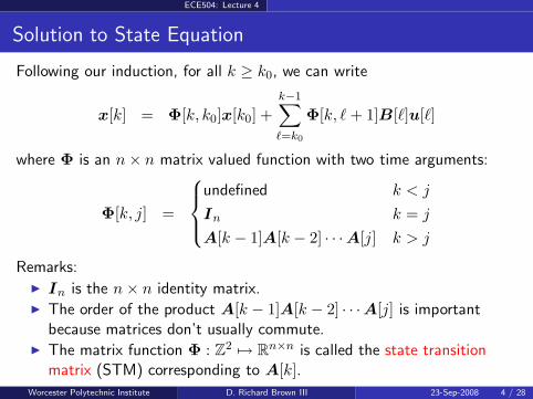
Following our induction, for all k ≥ k0, we can write
x[k] = Φ[k, k0]x[k0] +
k−1∑
ℓ=k0
Φ[k, ℓ + 1]B[ℓ]u[ℓ]
where Φ is an n × n matrix valued function with two time arguments:
Φ[k, j] =
undefined k < j
In k = j
A[k − 1]A[k − 2] · · ·A[j] k > j
Remarks:◮ In is the n × n identity matrix.◮ The order of the product A[k − 1]A[k − 2] · · ·A[j] is important
because matrices don’t usually commute.◮ The matrix function Φ : Z
2 7→ Rn×n is called the state transition
matrix (STM) corresponding to A[k].
Worcester Polytechnic Institute D. Richard Brown III 23-Sep-2008 4 / 28
ECE504: Lecture 4
Zero-Input Response
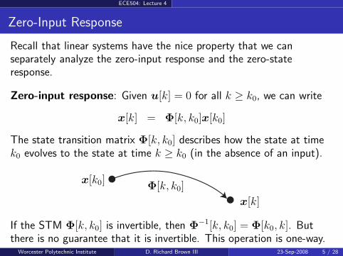
Recall that linear systems have the nice property that we canseparately analyze the zero-input response and the zero-stateresponse.
Zero-input response: Given u[k] = 0 for all k ≥ k0, we can write
x[k] = Φ[k, k0]x[k0]
The state transition matrix Φ[k, k0] describes how the state at timek0 evolves to the state at time k ≥ k0 (in the absence of an input).
x[k0]
x[k]
Φ[k, k0]
If the STM Φ[k, k0] is invertible, then Φ−1[k, k0] = Φ[k0, k]. But
there is no guarantee that it is invertible. This operation is one-way.Worcester Polytechnic Institute D. Richard Brown III 23-Sep-2008 5 / 28
ECE504: Lecture 4
Zero-State Response
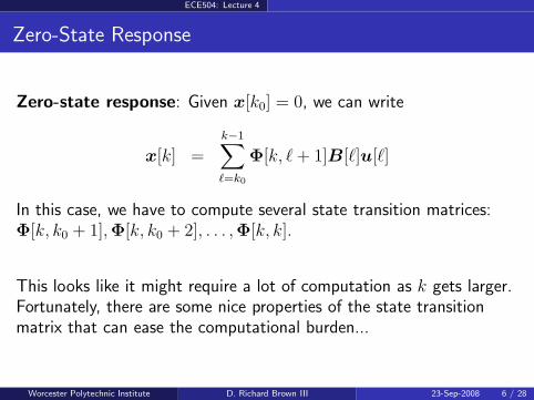
Zero-state response: Given x[k0] = 0, we can write
x[k] =
k−1∑
ℓ=k0
Φ[k, ℓ + 1]B[ℓ]u[ℓ]
In this case, we have to compute several state transition matrices:Φ[k, k0 + 1],Φ[k, k0 + 2], . . . ,Φ[k, k].
This looks like it might require a lot of computation as k gets larger.Fortunately, there are some nice properties of the state transitionmatrix that can ease the computational burden...
Worcester Polytechnic Institute D. Richard Brown III 23-Sep-2008 6 / 28
ECE504: Lecture 4
Some Basic Properties of the State Transition Matrix
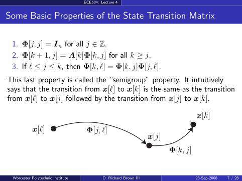
1. Φ[j, j] = In for all j ∈ Z.
2. Φ[k + 1, j] = A[k]Φ[k, j] for all k ≥ j.
3. If ℓ ≤ j ≤ k, then Φ[k, ℓ] = Φ[k, j]Φ[j, ℓ].
This last property is called the “semigroup” property. It intuitivelysays that the transition from x[ℓ] to x[k] is the same as the transitionfrom x[ℓ] to x[j] followed by the transition from x[j] to x[k].
x[ℓ]x[j]
x[k]
Φ[j, ℓ]
Φ[k, j]
Worcester Polytechnic Institute D. Richard Brown III 23-Sep-2008 7 / 28

ECE504: Lecture 4
Special Case: A[k] ≡ A for all k ≥ k0
When A[k] ≡ A for all k ≥ k0, the product
A[k − 1]A[k − 2] · · ·A[j] = AA · · ·A
How many A’s are involved in this product?
Hence, when A[k] ≡ A for all k ≥ k0, the state transition matrix can bewritten as
Φ[k, j] =
undefined k < j
In k = j
Ak−j k > j.
In this case, the solution to the DT state-update difference equation is
x[k] = Ak−k0x[k0] +
k−1∑
ℓ=k0
Ak−ℓ−1B[ℓ]u[ℓ]
for all k ≥ k0.Worcester Polytechnic Institute D. Richard Brown III 23-Sep-2008 8 / 28

ECE504: Lecture 4
Discrete-Time Output Solution
For all k ≥ k0, we can just plug our solution to the state equation into ourstate-space output equation to get
y[k] = C[k]Φ[k, k0]x[k0]︸ ︷︷ ︸
zero-input response
+ C[k]k−1∑
ℓ=k0
Φ[k, ℓ + 1]B[ℓ]u[ℓ] + D[k]u[k]
︸ ︷︷ ︸
zero-state response
If the system is time-invariant, then we can write
y[k] = CAk−k0x[k0]︸ ︷︷ ︸
zero-input response
+ C
k−1∑
ℓ=k0
Ak−ℓ−1Bu[ℓ] + Du[k]
︸ ︷︷ ︸
zero-state response
Worcester Polytechnic Institute D. Richard Brown III 23-Sep-2008 9 / 28

ECE504: Lecture 4
Remarks on Discrete-Time State-Space Solutions
For causal, linear, lumped discrete-time systems with p input terminals, q
output terminals, and n states, we have shown that, given x[k0] and u[k]for all k ≥ k0, there exists a unique solution to the discrete-timestate-update difference equation:
x[k] = Φ[k, k0]x[k0] +k−1∑
ℓ=k0
Φ[k, ℓ + 1]B[ℓ]u[ℓ]
for all k ≥ k0 with Φ[k, j] as defined earlier.
This also implies that, given x[k0] and u[k] for all k ≥ k0, there exists aunique solution to the discrete-time output equation.
Worcester Polytechnic Institute D. Richard Brown III 23-Sep-2008 10 / 28

ECE504: Lecture 4
Discrete-Time State-Space Example
Worcester Polytechnic Institute D. Richard Brown III 23-Sep-2008 11 / 28
ECE504: Lecture 4
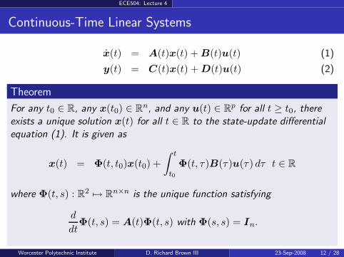
Continuous-Time Linear Systems
x(t) = A(t)x(t) + B(t)u(t) (1)
y(t) = C(t)x(t) + D(t)u(t) (2)
Theorem
For any t0 ∈ R, any x(t0) ∈ Rn, and any u(t) ∈ R
p for all t ≥ t0, thereexists a unique solution x(t) for all t ∈ R to the state-update differentialequation (1). It is given as
x(t) = Φ(t, t0)x(t0) +
∫ t
t0
Φ(t, τ)B(τ)u(τ) dτ t ∈ R
where Φ(t, s) : R2 7→ R
n×n is the unique function satisfying
d
dtΦ(t, s) = A(t)Φ(t, s) with Φ(s, s) = In.
Worcester Polytechnic Institute D. Richard Brown III 23-Sep-2008 12 / 28
ECE504: Lecture 4
Theorem Remarks
◮ Note that this theorem claims two things:
1. A solution to the state-update equation always exists.2. The solution is unique.
◮ Our strategy to prove the theorem:
1. We will first show that, given two solutions to thestate-update equation, they must be identical. Thisestablishes uniqueness.
2. We will then establish existence constructively by giving asolution and showing that it satisfies the state-updateequation.
Before doing any of this, however, we are going to need to learnsome more linear algebra (and a calculus refresher)...
Worcester Polytechnic Institute D. Richard Brown III 23-Sep-2008 13 / 28
ECE504: Lecture 4
Euclidean Norm of a Vector
Definition
For x ∈ Rn, the Euclidean norm of x is given as
‖x‖ :=(x2
1 + · · · + x2n
)1/2.
The Euclidean norm of vectors in R1, R
2, or R3 is just your normal notion
of distance/length.
Some useful facts (easy to show from the definition):
◮ ‖x‖2 = x⊤x.
◮ ‖αx‖ = |α|‖x‖ for any α in R.
◮ ‖x + y‖ ≤ ‖x‖ + ‖y‖ for any x ∈ Rn and any y ∈ R
n. This is oftencalled the triangle inequality.
Worcester Polytechnic Institute D. Richard Brown III 23-Sep-2008 14 / 28

ECE504: Lecture 4
Induced Euclidean Norm of a Matrix
Definition
For A ∈ Rn×n, the induced Euclidean norm of the matrix A is given as
‖A‖ := maxx∈Rn and ‖x‖=1
‖Ax‖.
◮ The set of vectors x where ‖x‖ = 1 is a unit-sphere in Rn.
◮ The induced Euclidean norm of A is the maximum value of ‖Ax‖ asx ranges over all points on this unit-sphere.
◮ Intuitively, ‖A‖ gives a measure of how much A can magnify thelength (Euclidean norm) of a vector in R
n.
Some useful facts (not too hard to show from the definition):◮ ‖A + B‖ ≤ ‖A‖ + ‖B‖ for any A ∈ R
n×n and any B ∈ Rn×n.
◮ ‖AB‖ ≤ ‖A‖‖B‖ for any A ∈ Rn×n and any B ∈ R
n×n.◮ ‖Ax‖ ≤ ‖A‖‖x‖ for any A ∈ R
n×n and any x ∈ Rn.
Worcester Polytechnic Institute D. Richard Brown III 23-Sep-2008 15 / 28

ECE504: Lecture 4
Schwarz Inequality
Theorem
Given x ∈ Rn and y ∈ R
n, then
|x⊤y| = |x1y1 + · · · + xnyn| ≤ ‖x‖‖y‖
Proof:
Worcester Polytechnic Institute D. Richard Brown III 23-Sep-2008 16 / 28
ECE504: Lecture 4
Leibniz’ rule
Theorem
If f(t, τ) is continuous and all of the necessary derivatives exist, then
d
dt
∫ w(t)
v(t)f(t, τ) dτ = w(t)f(t, w(t)) − v(t)f(t, v(t)) +
∫ w(t)
v(t)
d
dtf(t, τ) dτ
The proof can be found in most calculus textbooks.
Two particularly useful special cases are
d
dt
∫ t
af(τ) dτ = f(t)
d
dt
∫ a
tf(τ) dτ = −f(t)
where a is not a function of t.Worcester Polytechnic Institute D. Richard Brown III 23-Sep-2008 17 / 28

ECE504: Lecture 4
Back to the Theorem: Uniqueness Proof
x(t) = A(t)x(t) + B(t)u(t)
We first want to show that any solution x(t) to this state-updatedifferential equation must be unique.
To show this, suppose we had two solutions to the state-update differentialequation, x1(t) and x2(t) for t ∈ [s1, t1], both of which satisfy the initialcondition x1(t0) = x2(t0) = x(t0). Let’s prove that x1(t) must beidentical to x2(t)...
Worcester Polytechnic Institute D. Richard Brown III 23-Sep-2008 18 / 28

ECE504: Lecture 4
Theorem: Existence Proof Warmup
We now know that, if a solution to the state-update DE exists, it must beunique. We now need to show that a solution always exists.
To develop some intuition, let’s first assume that everything is scalar,i.e. p = q = n = 1. Our state update equation becomes
x(t) = a(t)x(t) + b(t)u(t)
Let
φ(t, s) := exp
{∫ t
sa(τ) dτ
}
What is φ(s, s)?
What is ddtφ(t, s)?
Worcester Polytechnic Institute D. Richard Brown III 23-Sep-2008 19 / 28

ECE504: Lecture 4
Theorem: Existence Proof Warmup
Note that φ(t, s) = exp{∫ t
s a(τ) dτ}
always exists and satisfies its own
differential equation:
d
dtφ(t, s) = a(t)φ(t, s) with φ(s, s) = 1.
Now lets try the following solution to the scalar state-update differentialequation with initial state condition x(t0):
x(t) = φ(t, t0)x(t0) +
∫ t
t0
φ(t, τ)b(τ)u(τ) dτ ∀t ∈ R
To see that this solution is valid, we should confirm two things:
1. Does our solution satisfy the initial condition requirement of thescalar state-update DE?
2. Does our solution really solve the scalar state-update DE?
Worcester Polytechnic Institute D. Richard Brown III 23-Sep-2008 20 / 28
ECE504: Lecture 4
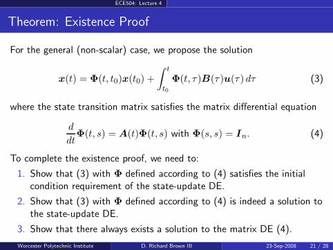
Theorem: Existence Proof
For the general (non-scalar) case, we propose the solution
x(t) = Φ(t, t0)x(t0) +
∫ t
t0
Φ(t, τ)B(τ)u(τ) dτ (3)
where the state transition matrix satisfies the matrix differential equation
d
dtΦ(t, s) = A(t)Φ(t, s) with Φ(s, s) = In. (4)
To complete the existence proof, we need to:
1. Show that (3) with Φ defined according to (4) satisfies the initialcondition requirement of the state-update DE.
2. Show that (3) with Φ defined according to (4) is indeed a solution tothe state-update DE.
3. Show that there always exists a solution to the matrix DE (4).
Worcester Polytechnic Institute D. Richard Brown III 23-Sep-2008 21 / 28
ECE504: Lecture 4
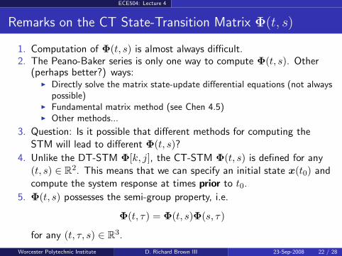
Remarks on the CT State-Transition Matrix Φ(t, s)
1. Computation of Φ(t, s) is almost always difficult.2. The Peano-Baker series is only one way to compute Φ(t, s). Other
(perhaps better?) ways:◮ Directly solve the matrix state-update differential equations (not always
possible)◮ Fundamental matrix method (see Chen 4.5)◮ Other methods...
3. Question: Is it possible that different methods for computing theSTM will lead to different Φ(t, s)?
4. Unlike the DT-STM Φ[k, j], the CT-STM Φ(t, s) is defined for any(t, s) ∈ R
2. This means that we can specify an initial state x(t0) andcompute the system response at times prior to t0.
5. Φ(t, s) possesses the semi-group property, i.e.
Φ(t, τ) = Φ(t, s)Φ(s, τ)
for any (t, τ, s) ∈ R3.
Worcester Polytechnic Institute D. Richard Brown III 23-Sep-2008 22 / 28

ECE504: Lecture 4
Important Special Case: A(t) ≡ A
When A(t) ≡ A, the state-transition matrix Peano-Baker series becomes
Φ(t, s) =∞∑
k=0
Mk(t, s)
=∞∑
k=0
∫ t
s
∫ τ1
s· · ·
∫ τk−1
sAA · · ·A︸ ︷︷ ︸
k−fold product
dτk · · · dτ1
=
∞∑
k=0
Ak
∫ t
s
∫ τ1
s· · ·
∫ τk−1
sdτk · · · dτ1
To compute Mk(t, s), let’s look at k = 0, 1, 2, . . . to see the pattern:
◮ What is M0(t, s)?
◮ What is M1(t, s)?
◮ What is M2(t, s)?
◮ What is M3(t, s)?
Worcester Polytechnic Institute D. Richard Brown III 23-Sep-2008 23 / 28
ECE504: Lecture 4
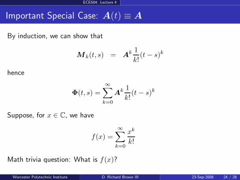
Important Special Case: A(t) ≡ A
By induction, we can show that
Mk(t, s) = Ak 1
k!(t − s)k
hence
Φ(t, s) =
∞∑
k=0
Ak 1
k!(t − s)k
Suppose, for x ∈ C, we have
f(x) =
∞∑
k=0
xk
k!
Math trivia question: What is f(x)?
Worcester Polytechnic Institute D. Richard Brown III 23-Sep-2008 24 / 28
ECE504: Lecture 4
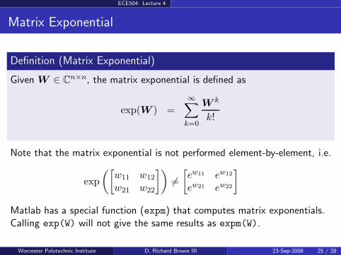
Matrix Exponential
Definition (Matrix Exponential)
Given W ∈ Cn×n, the matrix exponential is defined as
exp(W ) =∞∑
k=0
W k
k!
Note that the matrix exponential is not performed element-by-element, i.e.
exp
([w11 w12
w21 w22
])
6=
[ew11 ew12
ew21 ew22
]
Matlab has a special function (expm) that computes matrix exponentials.Calling exp(W) will not give the same results as expm(W).
Worcester Polytechnic Institute D. Richard Brown III 23-Sep-2008 25 / 28

ECE504: Lecture 4
Important Special Case: A(t) ≡ A
Putting it all together, when A(t) ≡ A, we can say that
Φ(t, s) = exp {(t − s)A}
Then the solution to the state-update DE is
x(t) = exp {(t − t0)A}x(t0) +
∫ t
t0
exp {(t − τ)A}B(τ)u(τ) dτ
and the output equation is
y(t) = C(t) exp {(t − t0)A}x(t0) + C(t)
Z
t
t0
exp {(t − τ )A}B(τ )u(τ ) dτ + D(t)u(t)
Worcester Polytechnic Institute D. Richard Brown III 23-Sep-2008 26 / 28

ECE504: Lecture 4
Contrast/Comparison Between CT and DT Solutions
Similarities
◮ Results have same “look”.
◮ Both have state transition matrices with same intuitive properties,e.g. semigroup.
Differences
◮ In DT systems, x[k] is only defined for k ≥ k0 because the DT-STMΦ[k, k0] is only defined for k ≥ k0.
◮ In CT systems, x(t) is only defined for all t ∈ R because the CT-STMΦ(t, t0) is defined for all (t, t0) ∈ R
2.
◮ We didn’t prove this, but the CT-STM Φ(t, t0) is always invertible.This is not true of the DT-STM Φ[k, k0].
Worcester Polytechnic Institute D. Richard Brown III 23-Sep-2008 27 / 28

ECE504: Lecture 4
Conclusions
◮ Solution to LTI or LTV discrete-time state-spacedifference equations (existence and uniqueness)
◮ Solution to LTI or LTV continuous-time state-spacedifferential equations (existence and uniqueness)
◮ Special case: time-invariant A matrix
◮ LTI discrete-time systems: Ak−j
◮ LTI continuous-time systems: exp{(t − τ)A}
Worcester Polytechnic Institute D. Richard Brown III 23-Sep-2008 28 / 28