ECE Department, University of IllinoisECE 552

Numerical Circuit Analysis

I. HajjSpring 2015

Lecture One

INTRODUCTION

Copyright © I. Hajj 2012 All rights reserved

Introduction

• System analysis is a basic step in system design

• Computer-Aided analysis or simulation helps in the design of complex systems before the systems are built or manufactured

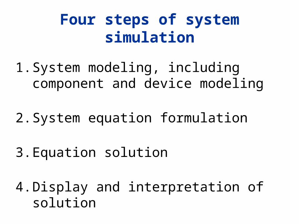
Four steps of system simulation

1. System modeling, including component and device modeling

2. System equation formulation

3. Equation solution

4. Display and interpretation of solution

Assumption

To start, we consider Electric Circuits that are modeled as interconnections of lumped elements (as opposed to distributed elements): Resistors; capacitors; inductors; independent sources.

We will not consider the derivation of device models in this course. We will assume that device models are provided. We will concentrate on equation formulation and equation solution techniques.

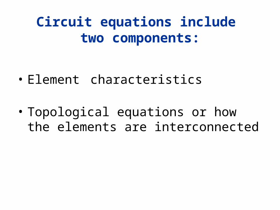
Circuit equations include two components:

• Element characteristics

• Topological equations or how the elements are interconnected

Types of Equations to be Solved

• Linear equations

• Nonlinear algebraic equations

• Differential-algebraic equations

• Partial differential equations (distributed elements)

Element Characteristics(Chapter 1)

Resistors

• Characterized by an algebraic relation between voltage v and current i

(Note the associated reference directions of v and i)

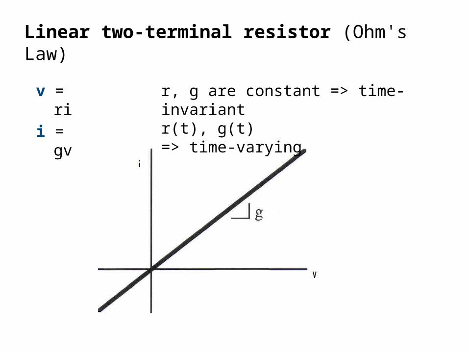
Linear two-terminal resistor (Ohm's Law)

v = ri

i = gv

r, g are constant => time-invariant r(t), g(t) => time-varying

Independent Sources

Current Sources Examples: i = 5 A, i = k sin ωt A

Independent Sources

Voltage Sources Examples: v = 5 V, v = B cos(ωt + Φ) V

Remark: Independent sources are characterized by an algebraic relationship

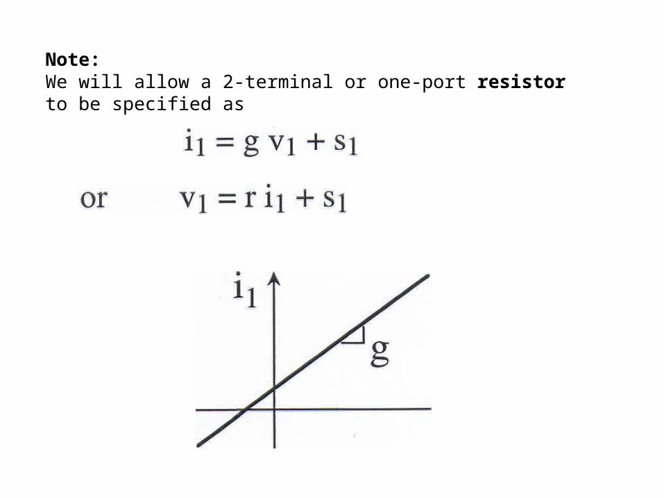
Note:We will allow a 2-terminal or one-port resistor to be specified as

Linear Multiterminal Resistors

i = [G]v, v = [R]i

or

If G, R, or H are constant matrices, then resistor is time-invariant; if they are functions of time, then resistor is time-variant.

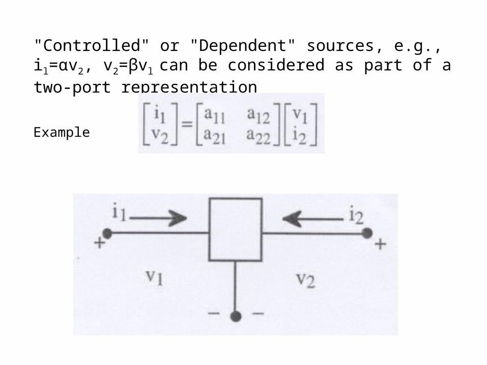
"Controlled" or "Dependent" sources, e.g., il=αv2, v2=βvl

can be considered as part of a two-port representation

Example

OR

General form of linear resistorcharacteristics, including dependent and independent sources is:

[G]v + [R]i = s

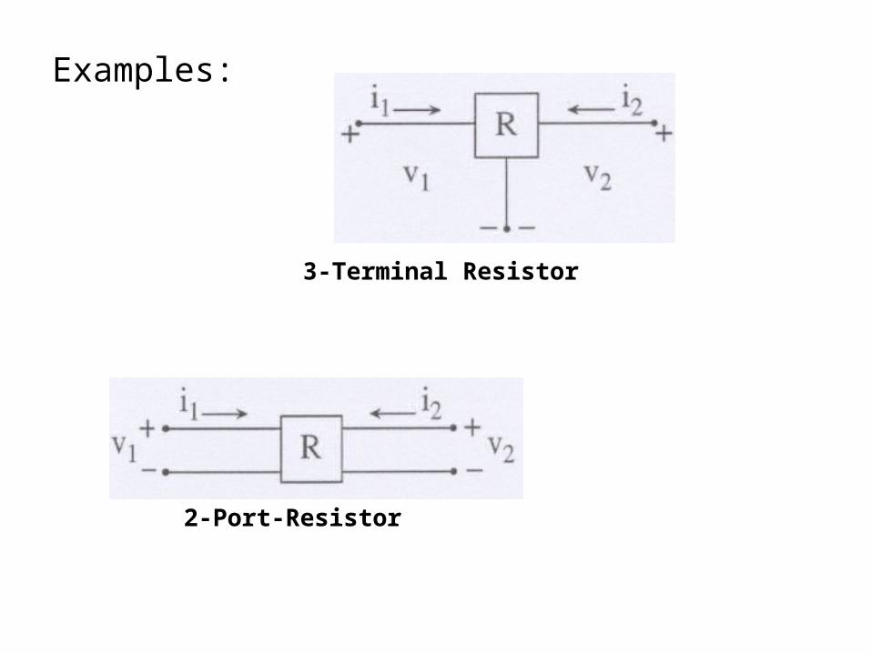
Examples:

3-Terminal Resistor

2-Port-Resistor

OR

Hybrid Representation

i1 = a11 v1 + a12i2 + s1

v2 = a21 v1 + a22i2 + s2

Matrix Form

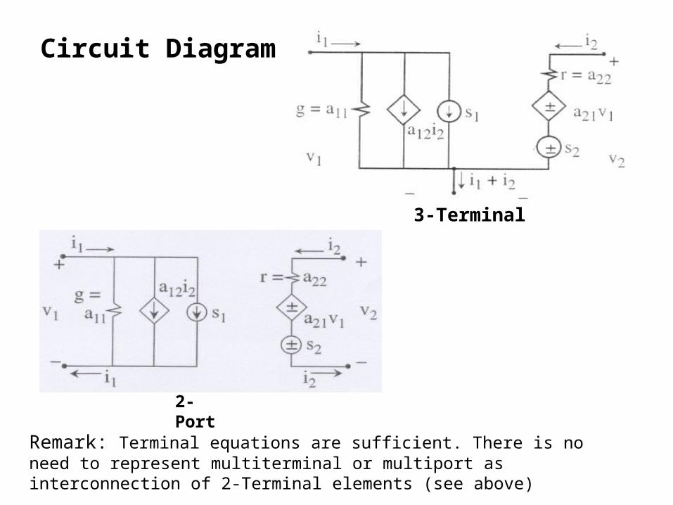
Circuit Diagram

3-Terminal

Remark: Terminal equations are sufficient. There is no need to represent multiterminal or multiport as interconnection of 2-Terminal elements (see above)

2-Port

Macromodeling (e.g. , Op-Amp)

Resistive macromodel

• Relation between voltages and currents at terminals or ports are derived from the internal equations.

• Internal voltages and currents of macromodel can be computed later, if desired. This leads the Hierarchical Analysis.

Nonlinear Resistors

Two terminals

i = g(v)

voltage-controlled

v

v

i

v

f(i,v) = 0

v = r(i)

current-controlled

v

or f ( i, v ) = 0

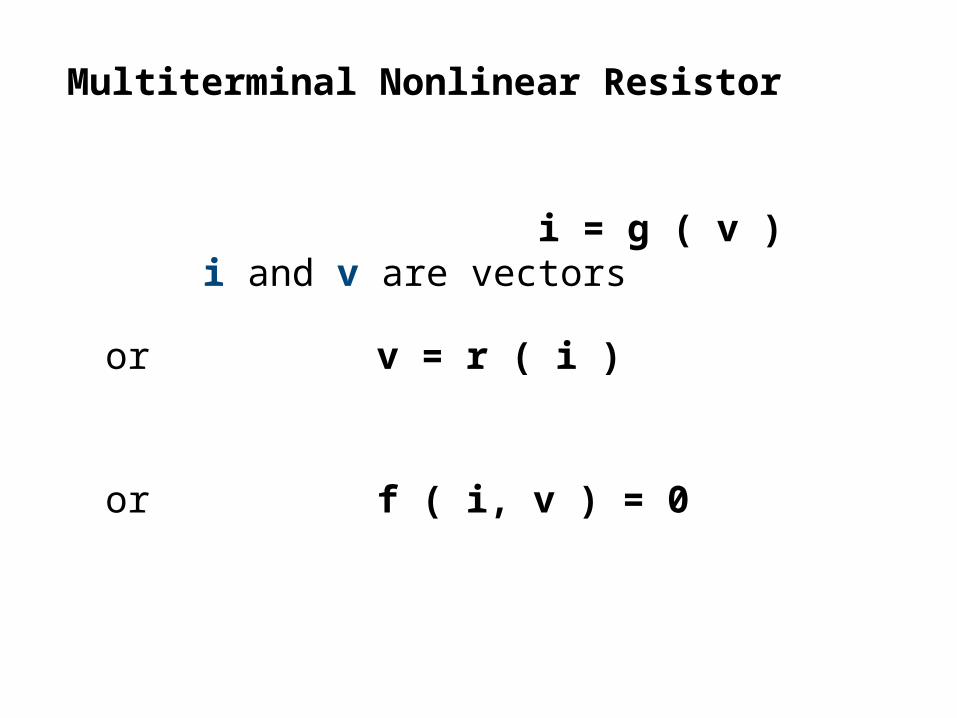
Multiterminal Nonlinear Resistor

or v = r ( i )

i = g ( v ) i and v are vectors

Linear, time-invariant

Time-varying linear capacitor

In steady-state sinusoidal analysis

Ic = ( jωC ) Vc

Capacitors

Multiterminal Linear Capacitors

Nonlinear Capacitors

vc = f(qc), f(vc,qc)=0

I1 = sC11 + sC12

I2 = sC21 + sC22

Symmetric case. However, there is no need to generate an equivalent circuit

Multiterminal Nonlinear

q

v

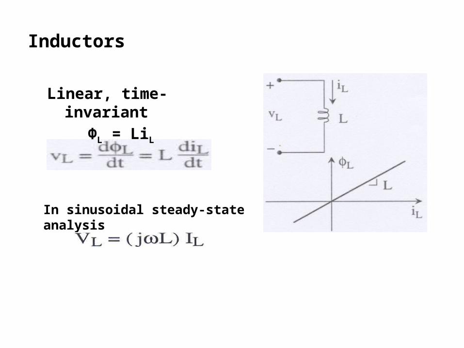
Inductors

Linear, time-invariant

ΦL = LiL

In sinusoidal steady-state analysis

Inductors

Time-varying linear inductor

Nonlinear Inductor

iL= f(ϕL), f(iL,ϕL)=0

Multiterminal Inductor

∅𝑳 = 𝑳 𝒊𝑳 (linear) ∅𝑳 = f (𝒊𝑳) (nonlinear) 𝒗𝑳 = 𝒅∅𝑳𝒅𝒕

∅𝑳 , 𝒊𝑳 , 𝒗𝑳 are vectors

L is a matrix

Linear Two-Port Inductor (Transformer)

𝒊𝟏 𝒊𝟐

+ • • +

𝒗𝟏 ∅𝟏 ∅𝟐 𝒗𝟐

_ _

ቈ∅𝟏∅𝟐 = 𝑳𝟏 𝑴

𝑴 𝑳𝟐൩ ቈ𝒊𝟏𝒊𝟐

𝒗𝟏𝒗𝟐൩ = 𝑳𝟏 𝑴

𝑴 𝑳𝟐൩ ൦𝒅𝒊𝟏𝒅𝒕𝒅𝒊𝟐𝒅𝒕൪

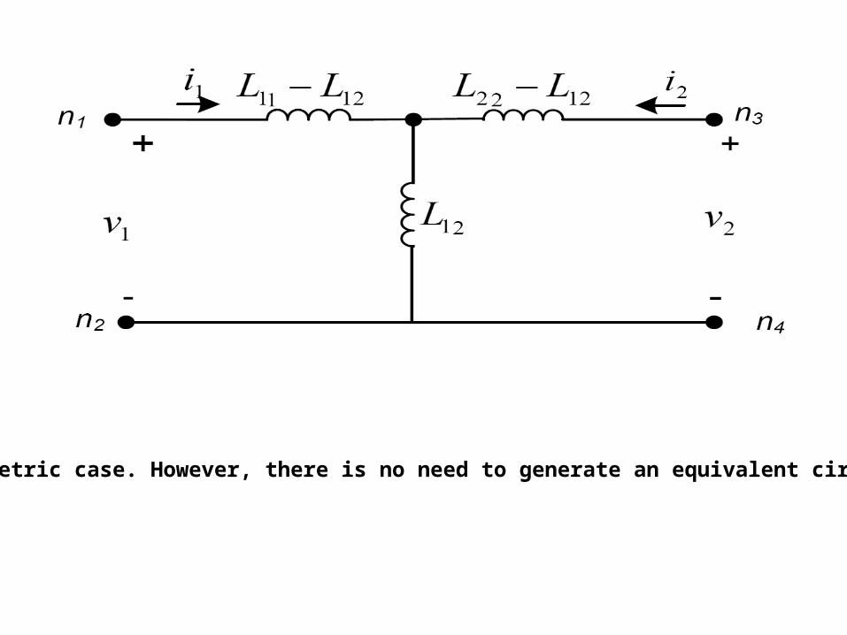
Symmetric case. However, there is no need to generate an equivalent circuit

Mem-Devices

• Charge-Controlled Memristor:ϕM(t) = fM(qM)

iM = dqM/dt, vM = dϕM/dt

• Flux-Controlled Memristor:qM(t) = fM(ϕM)

iM = dqM/dt, vM = dϕM/dt

Mem Systems

– Current-Controlled Memristive System: vM = f1(x,iM,t)iM(t)

dx/dt= f2(x,iM,t)

– Voltage-Controlled Memristive System: iM = f1(x,vM,t)vM(t)

dx/dt= f2(x,vM,t)

Memcapacitive Systems

• Voltage-Controlled Memcapacitive System:qM = f1(x,vM,t)vM(t)

iM = dqM/dt dx/dt= f2(x,vM,t)

• Charge-Controlled Memcapacitive System:vM = f1(x,qM,t)qM(t)

iM = dqM/dt dx/dt= f2(x,qM,t)

Meminductive Systems

• Current-Controlled Meminductive System:ϕM = f1(x,iM,t)iM(t)

vM = dϕM/dt dx/dt= f2(x,iM,t)

• Flux-Controlled Meminductive System:vM = f1(x,ϕM,t)ϕM(t)

iM = dqM/dt dx/dt= f2(x,ϕM,t)

Memdevices Symbols

f(i, v, q, φ, σ, ρ,x, ˙x, t) = 0,

f(i, v, q, φ,x, ˙x, t) = 0,

General Element