ECE 645 – Hypothesis Testing

J. V. Krogmeier

February 10, 2014

Contents

1 Hypothesis Testing / Detection Setup 4

2 Bayesian Hypothesis Testing 6

2.1 Derivation of the Bayes rule for M = 2 . . . . . . . . . . . . . . . . . . . 8

2.2 Other forms for the Bayes rule for M = 2 . . . . . . . . . . . . . . . . . . 13

2.3 Bayes ⇔ Minimum Prob. of Error for Uniform Costs . . . . . . . . . . . 14

2.4 Interpretation as Posterior Costs . . . . . . . . . . . . . . . . . . . . . . 15

2.5 Example: Location Testing with Gaussian Error . . . . . . . . . . . . . . 17

1

2.6 Example: Location Testing with Gaussian Error for IID Case . . . . . . . 19

2.7 Example: Non-Gaussian . . . . . . . . . . . . . . . . . . . . . . . . . . . 23

3 Neyman-Pearson Hypothesis Testing 26

3.1 Example: A common sense argument for NP solution . . . . . . . . . . . 28

3.2 The Neyman-Pearson Lemma . . . . . . . . . . . . . . . . . . . . . . . . 29

3.3 Proof of the Neyman-Pearson Lemma . . . . . . . . . . . . . . . . . . . . 30

3.4 Example: Location Testing with Gaussian Error . . . . . . . . . . . . . . 43

3.5 Example: Discrete Detection . . . . . . . . . . . . . . . . . . . . . . . . 48

Hypothesis Testing 2

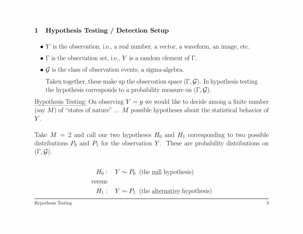
1 Hypothesis Testing / Detection Setup

• Y is the observation, i.e., a real number, a vector, a waveform, an image, etc.

• Γ is the observation set, i.e., Y is a random element of Γ.

• G is the class of observation events, a sigma-algebra.

Taken together, these make up the observation space (Γ,G). In hypothesis testing

the hypothesis corresponds to a probability measure on (Γ,G).

Hypothesis Testing: On observing Y = y we would like to decide among a finite number

(say M) of “states of nature” ... M possible hypotheses about the statistical behavior of

Y .

Take M = 2 and call our two hypotheses H0 and H1 corresponding to two possible

distributions P0 and P1 for the observation Y . These are probability distributions on

(Γ,G).

H0 : Y ∼ P0 (the null hypothesis)

versus

H1 : Y ∼ P1 (the alternative hypothesis)

Hypothesis Testing 3

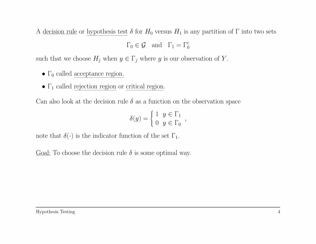
A decision rule or hypothesis test δ for H0 versus H1 is any partition of Γ into two sets

Γ0 ∈ G and Γ1 = Γc0

such that we choose Hj when y ∈ Γj where y is our observation of Y .

• Γ0 called acceptance region.

• Γ1 called rejection region or critical region.

Can also look at the decision rule δ as a function on the observation space

δ(y) =

1 y ∈ Γ1

0 y ∈ Γ0,

note that δ(·) is the indicator function of the set Γ1.

Goal: To choose the decision rule δ is some optimal way.

Hypothesis Testing 4

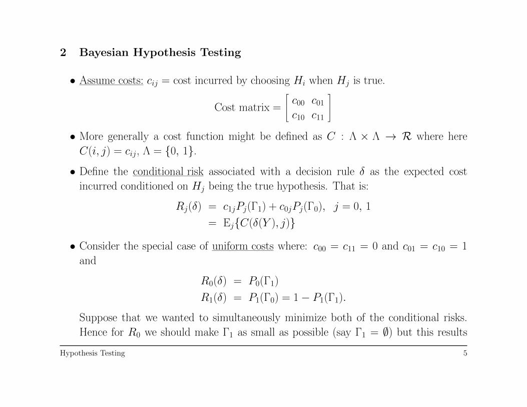
2 Bayesian Hypothesis Testing

• Assume costs: cij = cost incurred by choosing Hi when Hj is true.

Cost matrix =

c00 c01

c10 c11

• More generally a cost function might be defined as C : Λ × Λ → R where here

C(i, j) = cij, Λ = {0, 1}.

• Define the conditional risk associated with a decision rule δ as the expected cost

incurred conditioned on Hj being the true hypothesis. That is:

Rj(δ) = c1jPj(Γ1) + c0jPj(Γ0), j = 0, 1

= Ej{C(δ(Y ), j)}

• Consider the special case of uniform costs where: c00 = c11 = 0 and c01 = c10 = 1

and

R0(δ) = P0(Γ1)

R1(δ) = P1(Γ0) = 1− P1(Γ1).

Suppose that we wanted to simultaneously minimize both of the conditional risks.

Hence for R0 we should make Γ1 as small as possible (say Γ1 = ∅) but this results

Hypothesis Testing 5

inevitably in a large R1. On the other hand, starting from R1 we should like Γ0 to

be as small as possible (say Γ0 = ∅) ... then R0 is large. These requirements conflict

and so we cannot simultaneously minimize.

• A way out is to introduce priors in a Bayesian framework in order to find a single

average criterion for minimization.

• Therefore assume we know the prior probabilities of the two hypotheses (i.e., without

knowledge of the actual observation): πj = the probability with which Hj occurs,

unconditioned on an observation. Note

* π0 + π1 = 1

* π0, π1 ≥ 0

• Define the Bayes risk or average risk as the unconditional expected cost:

r(δ) = π0R0(δ) + π1R1(δ)

= E{EJ{C(δ(Y ), J)}}

where we have defined J to be a discrete rv taking values j = 0, 1 with the probabil-

ities π0 and π1, respectively. We only write it this way to emphasize that the Bayes

risk is the expectation of a conditional expectation an observation made later on in

discussing Bayesian estimation.

Hypothesis Testing 6

• Then define an optimal decision rule for H0 vs. H1 to be one minimizing r(δ). Such

a minimizing rule is called a Bayes rule.

2.1 Derivation of the Bayes rule for M = 2

Hypothesis Testing 7

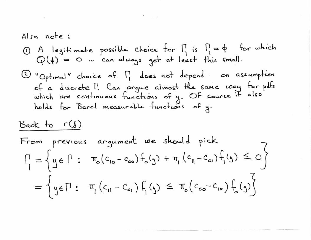
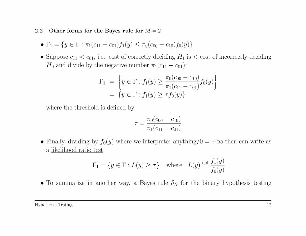
2.2 Other forms for the Bayes rule for M = 2

• Γ1 = {y ∈ Γ : π1(c11 − c01)f1(y) ≤ π0(c00 − c10)f0(y)}

• Suppose c11 < c01, i.e., cost of correctly deciding H1 is < cost of incorrectly deciding

H0 and divide by the negative number π1(c11 − c01):

Γ1 =

y ∈ Γ : f1(y) ≥ π0(c00 − c10)

π1(c11 − c01)f0(y)

= {y ∈ Γ : f1(y) ≥ τf0(y)}

where the threshold is defined by

τ =π0(c00 − c10)

π1(c11 − c01).

• Finally, dividing by f0(y) where we interprete: anything/0 = +∞ then can write as

a likelihood ratio test

Γ1 = {y ∈ Γ : L(y) ≥ τ} where L(y) def=f1(y)

f0(y)

• To summarize in another way, a Bayes rule δB for the binary hypothesis testing

Hypothesis Testing 12

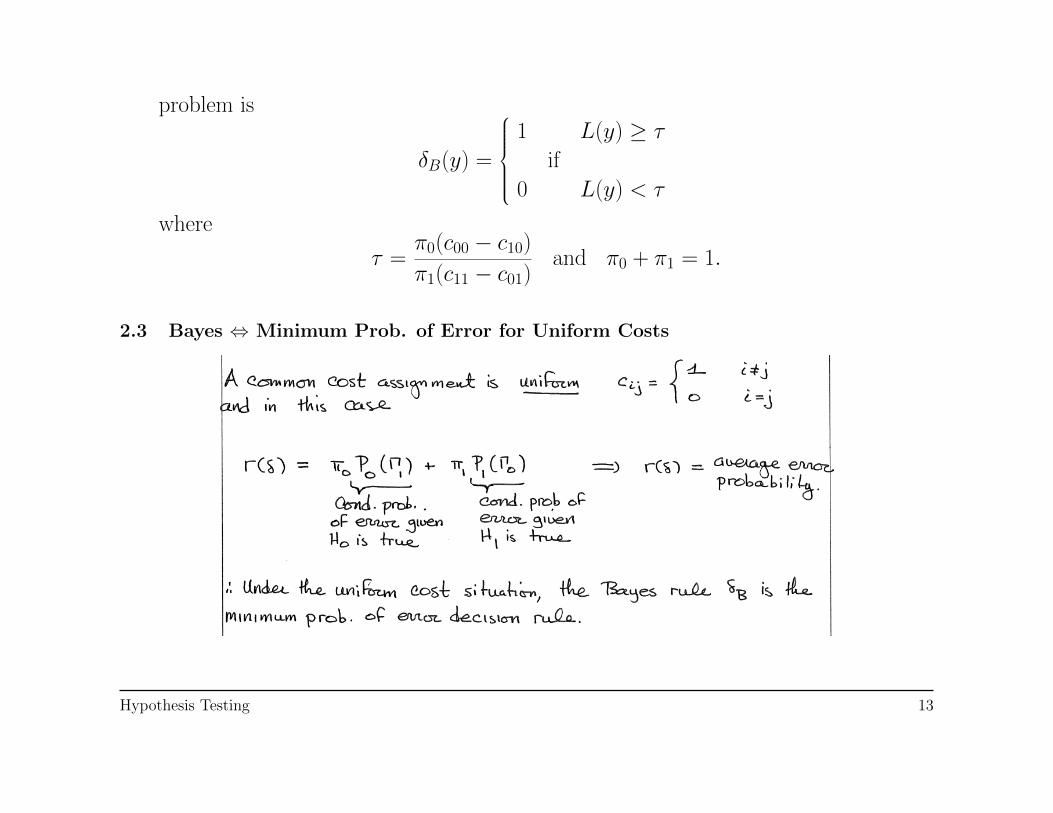
problem is

δB(y) =

1 L(y) ≥ τ

if

0 L(y) < τ

where

τ =π0(c00 − c10)

π1(c11 − c01)and π0 + π1 = 1.

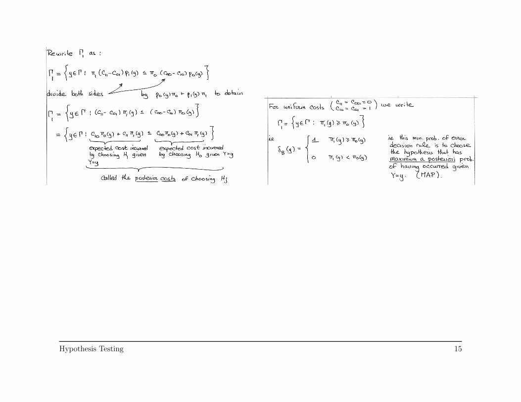
2.3 Bayes ⇔ Minimum Prob. of Error for Uniform Costs

Hypothesis Testing 13

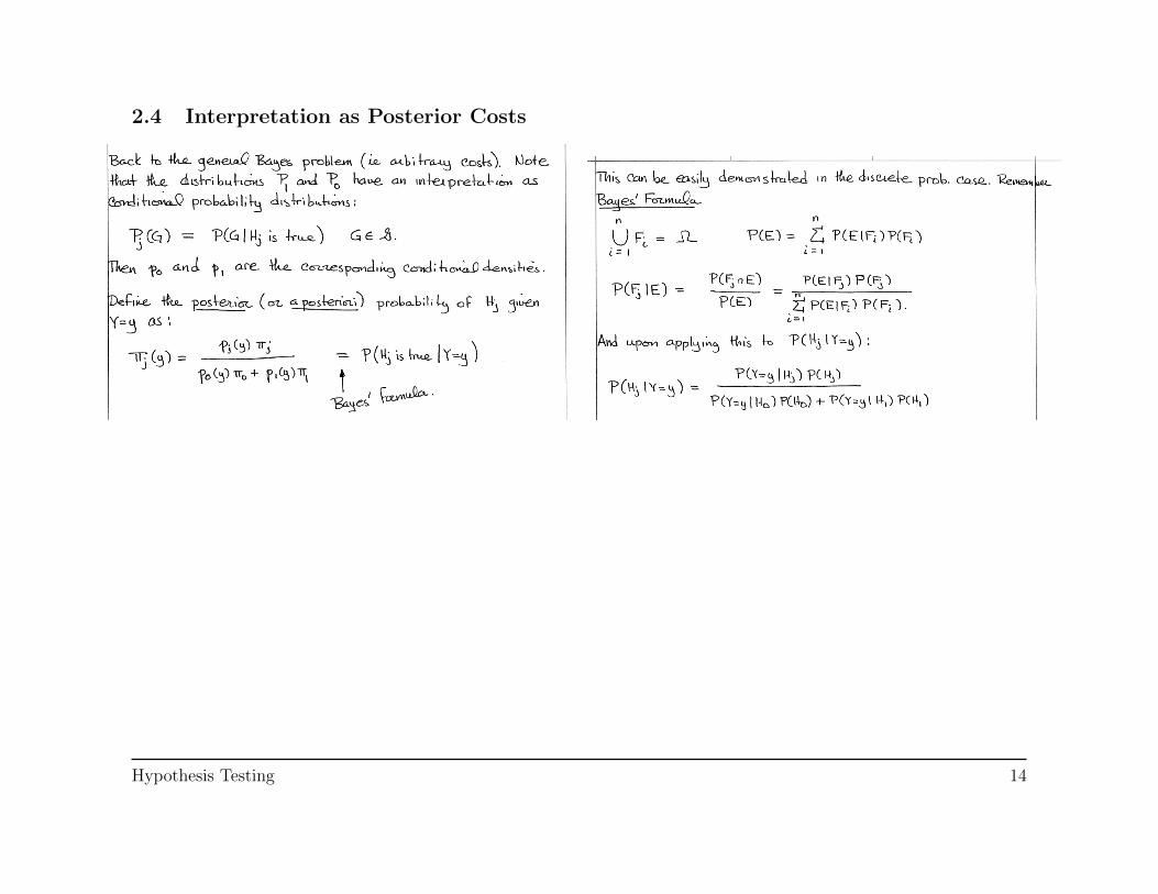
2.4 Interpretation as Posterior Costs

Hypothesis Testing 14

Hypothesis Testing 15

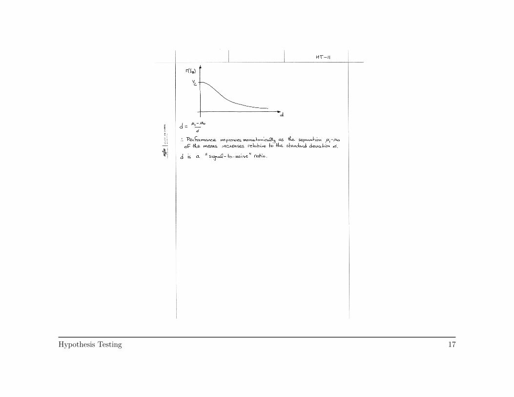
2.5 Example: Location Testing with Gaussian Error

Hypothesis Testing 16

Hypothesis Testing 17

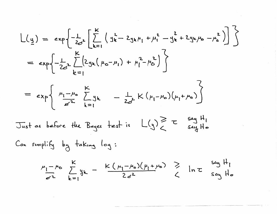
2.6 Example: Location Testing with Gaussian Error for IID Case

Hypothesis Testing 18

2.7 Example: Non-Gaussian

Hypothesis Testing 22

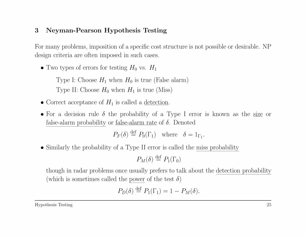
3 Neyman-Pearson Hypothesis Testing

For many problems, imposition of a specific cost structure is not possible or desirable. NP

design criteria are often imposed in such cases.

• Two types of errors for testing H0 vs. H1

Type I: Choose H1 when H0 is true (False alarm)

Type II: Choose H0 when H1 is true (Miss)

• Correct acceptance of H1 is called a detection.

• For a decision rule δ the probability of a Type I error is known as the size or

false-alarm probability or false-alarm rate of δ. Denoted

PF (δ) def= P0(Γ1) where δ = 1Γ1.

• Similarly the probability of a Type II error is called the miss probability

PM(δ) def= P1(Γ0)

though in radar problems once usually prefers to talk about the detection probability

(which is sometimes called the power of the test δ)

PD(δ) def= P1(Γ1) = 1− PM(δ).

Hypothesis Testing 25

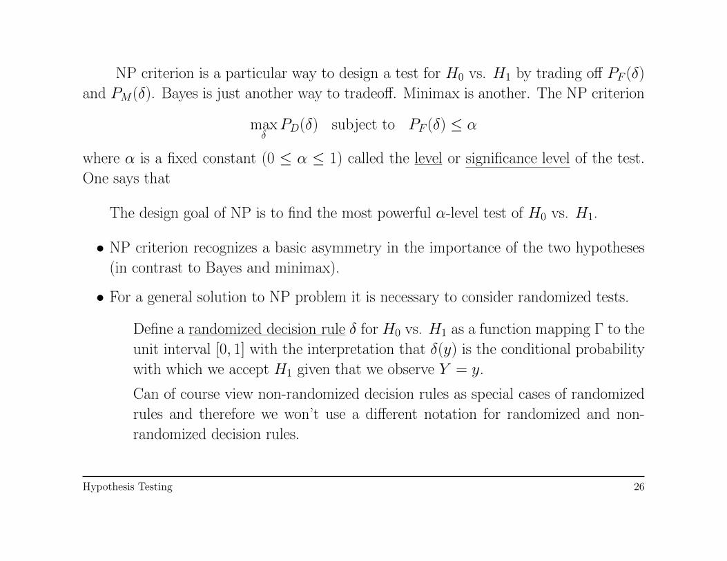
NP criterion is a particular way to design a test for H0 vs. H1 by trading off PF (δ)

and PM(δ). Bayes is just another way to tradeoff. Minimax is another. The NP criterion

maxδPD(δ) subject to PF (δ) ≤ α

where α is a fixed constant (0 ≤ α ≤ 1) called the level or significance level of the test.

One says that

The design goal of NP is to find the most powerful α-level test of H0 vs. H1.

• NP criterion recognizes a basic asymmetry in the importance of the two hypotheses

(in contrast to Bayes and minimax).

• For a general solution to NP problem it is necessary to consider randomized tests.

Define a randomized decision rule δ for H0 vs. H1 as a function mapping Γ to the

unit interval [0, 1] with the interpretation that δ(y) is the conditional probability

with which we accept H1 given that we observe Y = y.

Can of course view non-randomized decision rules as special cases of randomized

rules and therefore we won’t use a different notation for randomized and non-

randomized decision rules.

Hypothesis Testing 26

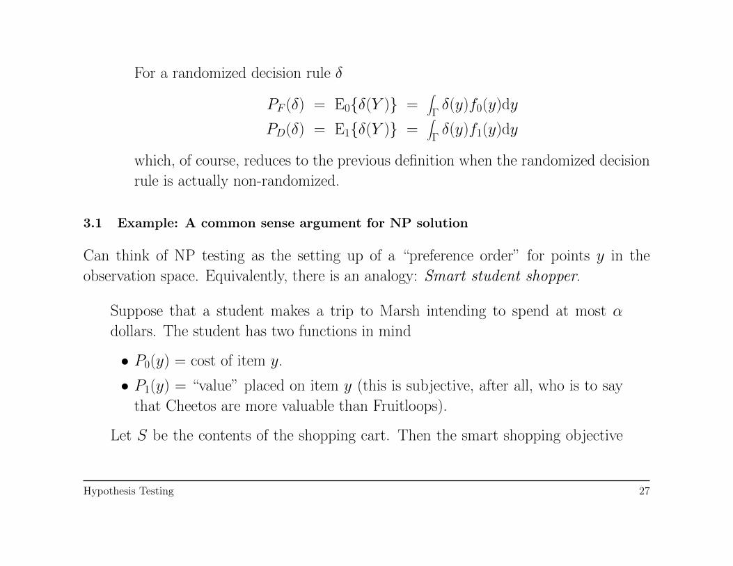
For a randomized decision rule δ

PF (δ) = E0{δ(Y )} =∫Γδ(y)f0(y)dy

PD(δ) = E1{δ(Y )} =∫Γδ(y)f1(y)dy

which, of course, reduces to the previous definition when the randomized decision

rule is actually non-randomized.

3.1 Example: A common sense argument for NP solution

Can think of NP testing as the setting up of a “preference order” for points y in the

observation space. Equivalently, there is an analogy: Smart student shopper.

Suppose that a student makes a trip to Marsh intending to spend at most α

dollars. The student has two functions in mind

• P0(y) = cost of item y.

• P1(y) = “value” placed on item y (this is subjective, after all, who is to say

that Cheetos are more valuable than Fruitloops).

Let S be the contents of the shopping cart. Then the smart shopping objective

Hypothesis Testing 27

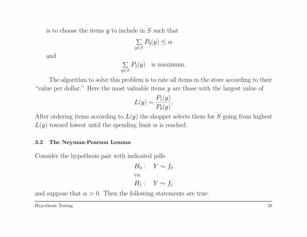
is to choose the items y to include in S such that∑y∈S

P0(y) ≤ α

and ∑y∈S

P1(y) is maximum.

The algorithm to solve this problem is to rate all items in the store according to their

“value per dollar.” Here the most valuable items y are those with the largest value of

L(y) =P1(y)

P0(y).

After ordering items according to L(y) the shopper selects them for S going from highest

L(y) toward lowest until the spending limit α is reached.

3.2 The Neyman-Pearson Lemma

Consider the hypothesis pair with indicated pdfs

H0 : Y ∼ f0

vs.

H1 : Y ∼ f1

and suppose that α > 0. Then the following statements are true.

Hypothesis Testing 28

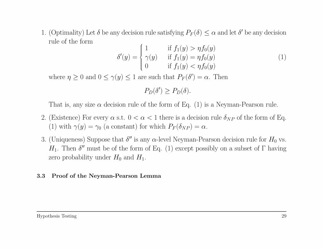
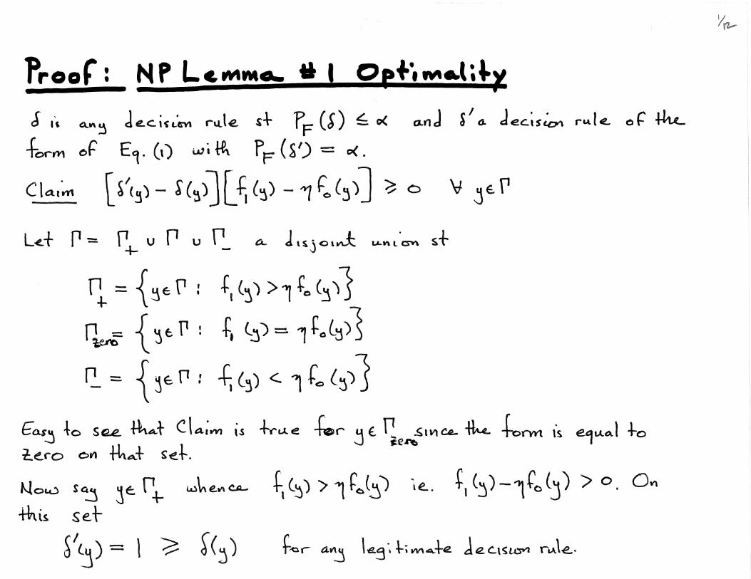
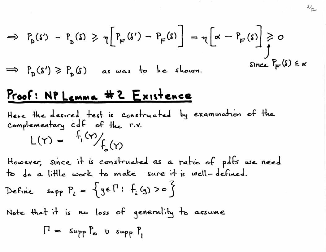
1. (Optimality) Let δ be any decision rule satisfying PF (δ) ≤ α and let δ′ be any decision

rule of the form

δ′(y) =

1 if f1(y) > ηf0(y)

γ(y) if f1(y) = ηf0(y)

0 if f1(y) < ηf0(y)

(1)

where η ≥ 0 and 0 ≤ γ(y) ≤ 1 are such that PF (δ′) = α. Then

PD(δ′) ≥ PD(δ).

That is, any size α decision rule of the form of Eq. (1) is a Neyman-Pearson rule.

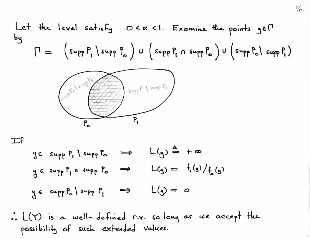
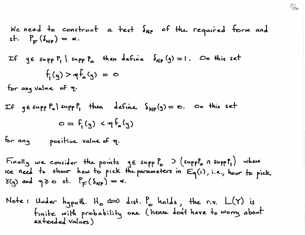
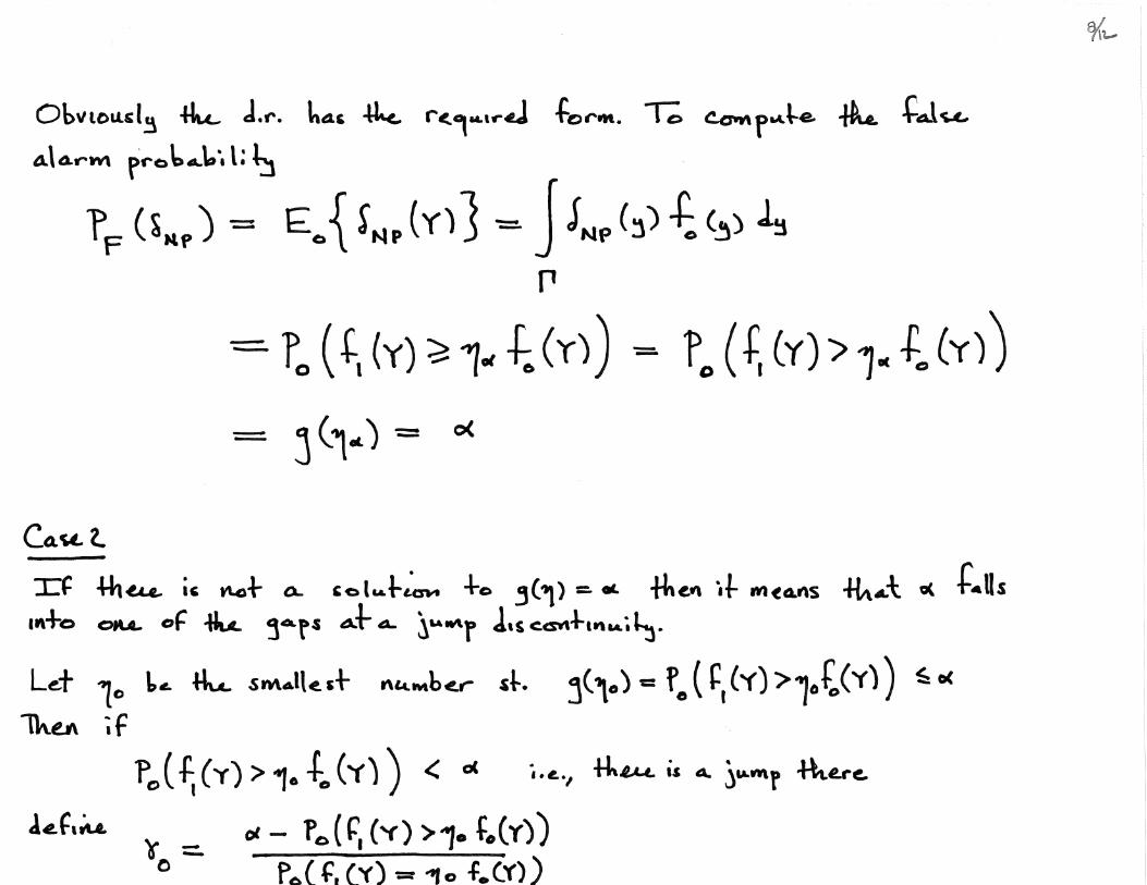
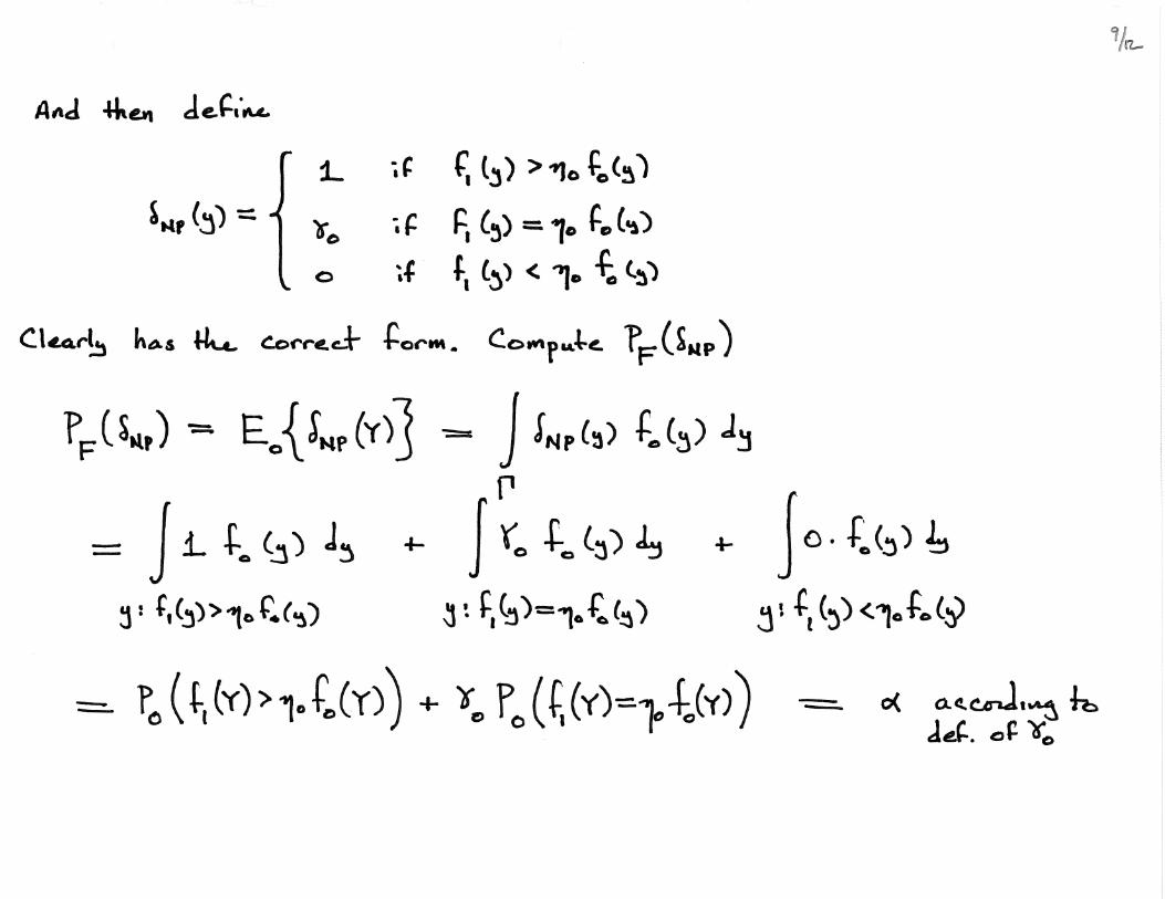
2. (Existence) For every α s.t. 0 < α < 1 there is a decision rule δNP of the form of Eq.

(1) with γ(y) = γ0 (a constant) for which PF (δNP ) = α.

3. (Uniqueness) Suppose that δ′′ is any α-level Neyman-Pearson decision rule for H0 vs.

H1. Then δ′′ must be of the form of Eq. (1) except possibly on a subset of Γ having

zero probability under H0 and H1.

3.3 Proof of the Neyman-Pearson Lemma

Hypothesis Testing 29

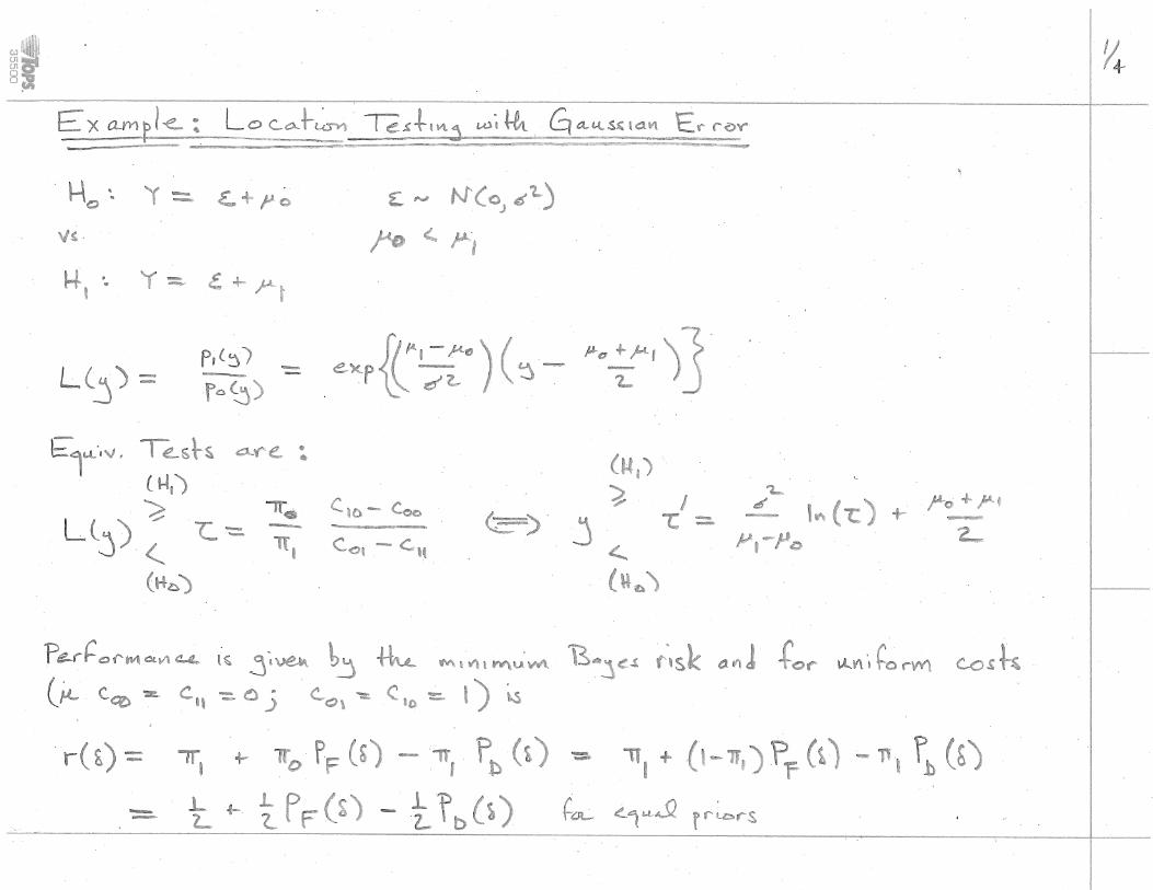
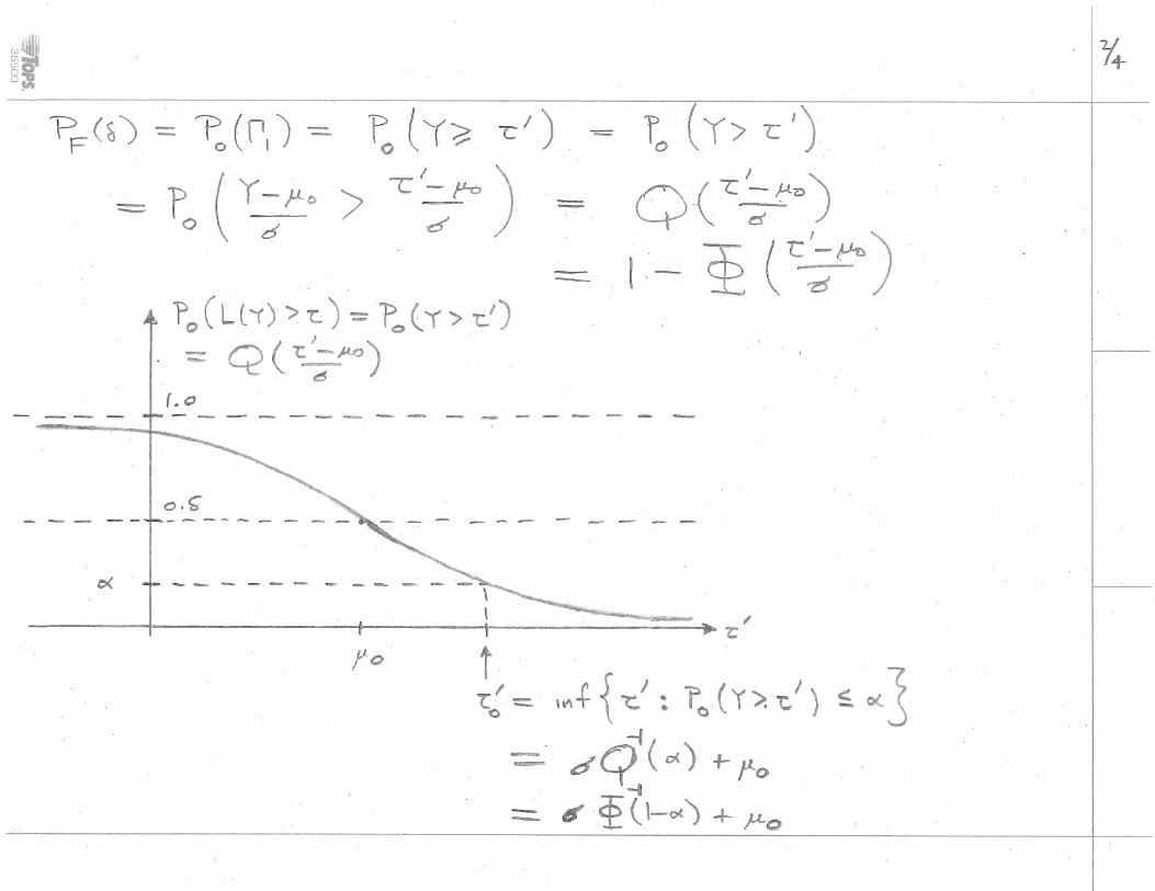
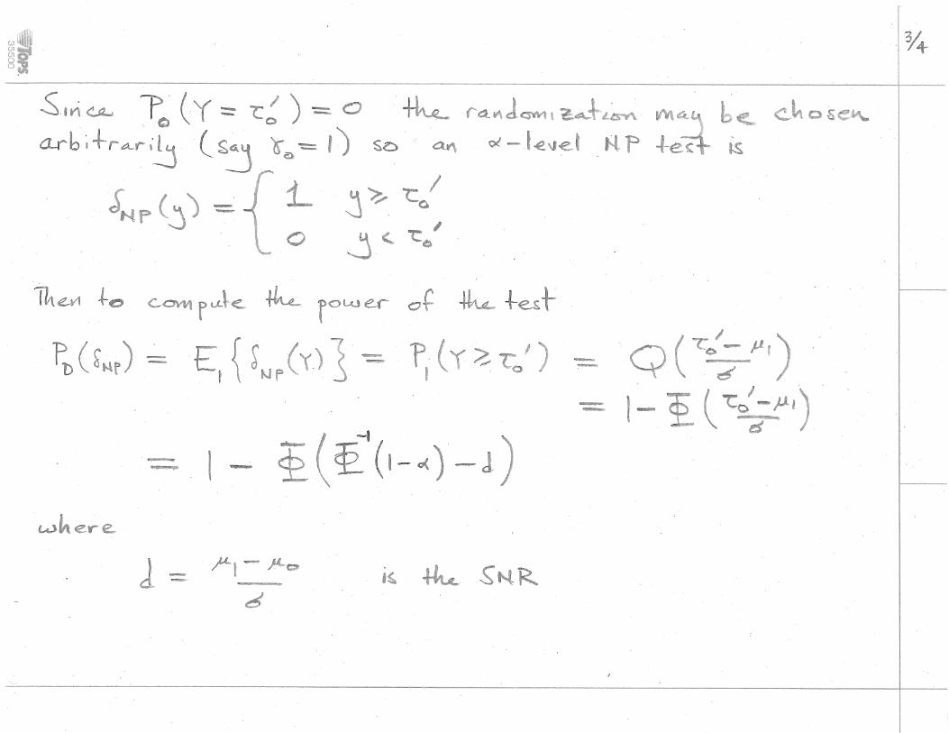
3.4 Example: Location Testing with Gaussian Error

Hypothesis Testing 42

3.5 Example: Discrete Detection

Hypothesis Testing 47