ESE566A Modern System-on-Chip Design, Spring 2017

ECE 566A Modern System-on-Chip Design, Spring 2017 Class Project: CNN hardware accelerator design

1. Overview ..................................................................................................................................... 1

2. Background knowledge .............................................................................................................. 1

2.1 Convolutional neural network brief introduction ................................................................. 1

2.2 CNN summarized in 4 steps ................................................................................................. 2

2.3 MNIST Dataset ..................................................................................................................... 4

3. Introduction of CNN source code C/C++ ................................................................................... 4

3.1 Code structure ....................................................................................................................... 5

3.2 Explanation of each layer...................................................................................................... 5

3.3 Forward propagation process ................................................................................................ 7

3.4 Error back propagation process ............................................................................................ 7

3.5 Matlab reference resource ..................................................................................................... 8

4. Possible optimizations using parallelism in referenced C/C++ code ......................................... 8

5. How to get started ....................................................................................................................... 9

6. Required Project Deliverables .................................................................................................. 10

6.1 Basic functionality .............................................................................................................. 10

6.2 Performance expectation ..................................................................................................... 10

6.3 Report expectation .............................................................................................................. 11

7. Project submission .................................................................................................................... 12

8. Acknowledgement .................................................................................................................... 12

Appendix A ................................................................................................................................... 13

ESE566A Modern System-on-Chip Design, Spring 2017

1

1. Overview

Convolutional neural networks have been widely employed for image recognition

applications because of their high accuracy, which they achieve by emulating how our

own brain recognizes objects. The possibility of making our electronic devices recognize

their surroundings have spawned a vast number potential of useful applications,

including video surveillance, mobile robot vision, image search in data centers, and

more. The increasing usage of such applications in mobile platforms and data centers

have led to a higher demands for methods that can compute these computational-

insensitive networks in a fast and power efficient way. One such method is by using

application specific hardware accelerators.

This project will explore the design and implementation of convolutional neural networks

(CNNs) in hardware with the intention of improving energy efficiency over traditional

implementation in software on a general-purpose CPU. The overall goal is to build an

energy efficient hardware accelerator that implements the forward propagation in CNN

to recognize the MNIST handwriting dataset.

2. Background knowledge

2.1 Convolutional neural network brief introduction

Convolutional Neural Networks (CNN), is a type of advanced artificial neural network. It differs from regular neural networks in terms of the flow of signals between neurons. Typical neural networks pass signals along the input-output channel in a single direction, without allowing signals to loop back into the network. This is called a forward feed. While forward feed networks were successfully employed for image and text recognition, it required all neurons to be connected, resulting in an overly-complex network structure. The cost of complexity grows when the network has to be trained on large datasets which, coupled with the limitations of computer processing speeds, result in grossly long training times. Hence, forward feed networks have fallen into disuse from mainstream machine learning in today’s high resolution, high bandwidth, mass media age. A new solution was needed. In 1986, researchers Hubel and Wiesel were examining a cat’s visual cortex when they discovered that its receptive field comprised sub-regions which were layered over each other to cover the entire visual field. These layers act as filters that process input images, which are then passed on to subsequent layers. This proved to be a simpler and more efficient way to carry signals. In 1998, Yann LeCun and Yoshua Bengio tried to capture the organization of neurons in the cat’s visual cortex as a form of artificial neural net, establishing the basis of the first CNN.

ESE566A Modern System-on-Chip Design, Spring 2017

2

2.2 CNN summarized in 4 steps

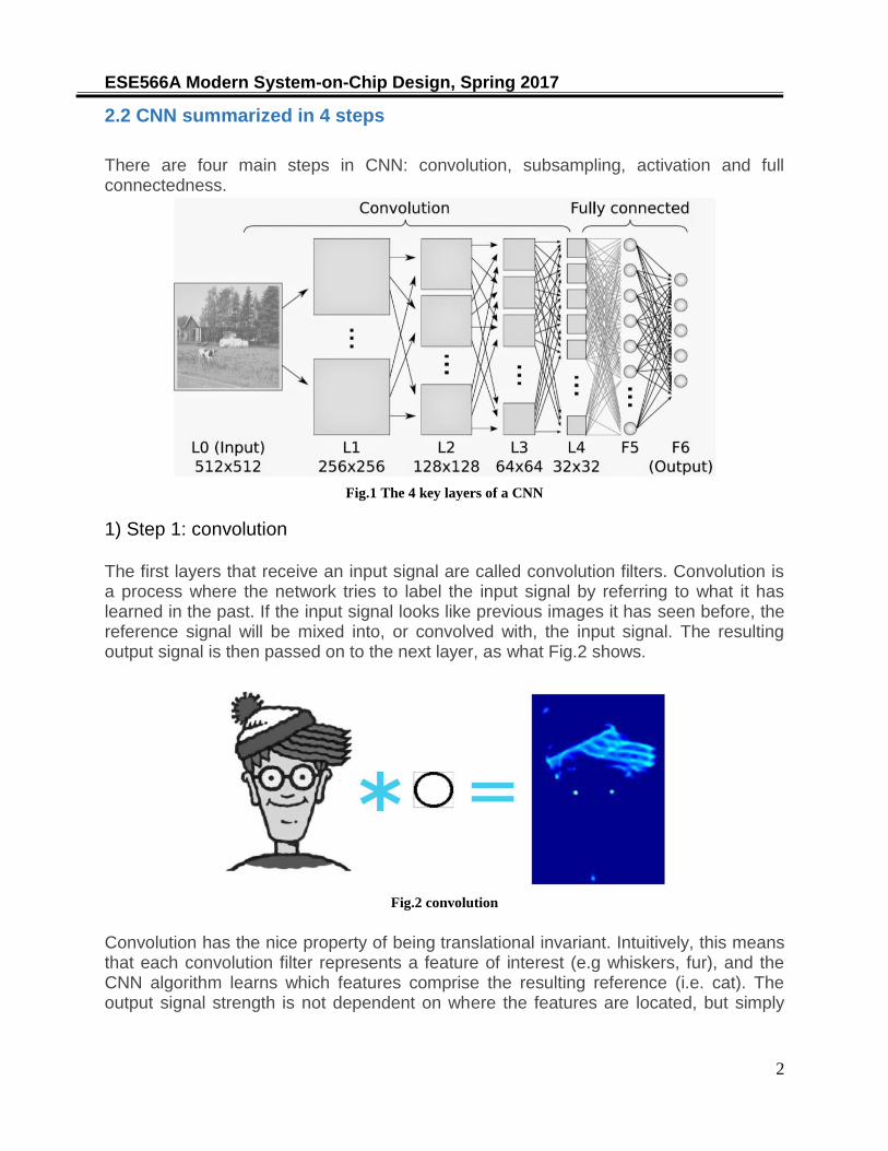
There are four main steps in CNN: convolution, subsampling, activation and full connectedness.

Fig.1 The 4 key layers of a CNN

1) Step 1: convolution The first layers that receive an input signal are called convolution filters. Convolution is a process where the network tries to label the input signal by referring to what it has learned in the past. If the input signal looks like previous images it has seen before, the reference signal will be mixed into, or convolved with, the input signal. The resulting output signal is then passed on to the next layer, as what Fig.2 shows.

Fig.2 convolution

Convolution has the nice property of being translational invariant. Intuitively, this means that each convolution filter represents a feature of interest (e.g whiskers, fur), and the CNN algorithm learns which features comprise the resulting reference (i.e. cat). The output signal strength is not dependent on where the features are located, but simply

ESE566A Modern System-on-Chip Design, Spring 2017

3

whether the features are present. Hence, a cat could be sitting in different positions, and the CNN algorithm would still be able to recognize it. 2) Step 2: Subsampling Inputs from the convolution layer can be “smoothened” to reduce the sensitivity of the filters to noise and variations. This smoothing process is called subsampling, and can be achieved by taking averages or taking the maximum over a sample of the signal. Examples of subsampling methods (for image signals) include reducing the size of the image, or reducing the color contrast across red, green, blue (RGB) channels.

Fig.3 Subsampling

3) Step 3: Activation The activation layer controls how the signal flows from one layer to the next, emulating how neurons are fired in our brain. Output signals which are strongly associated with past references would activate more neurons, enabling signals to be propagated more efficiently for identification. CNN is compatible with a wide variety of complex activation functions to model signal propagation, the most common function being the Rectified Linear Unit (ReLU), which is favored for its faster training speed. 4) Step4: Fully connected The last layers in the network are fully connected, meaning that neurons of preceding layers are connected to every neuron in subsequent layers. This mimics high level reasoning where all possible pathways from the input to output are considered. 5) Step 5: Loss (During training step) When training the neural network, there is additional layer called the loss layer. This layer provides feedback to the neural network on whether it identified inputs correctly,

ESE566A Modern System-on-Chip Design, Spring 2017

4

and if not, how far off its guesses were. This helps to guide the neural network to reinforce the right concepts as it trains. This is always the last layer during training.

2.3 MNIST Dataset

The MNIST database of handwritten digits, available from this page, has a training set of 60,000 examples, and a test set of 10,000 examples. It is a subset of a larger set available from NIST. The digits have been size-normalized and centered in a fixed-size image. It is a good database for people who want to try learning techniques and pattern recognition methods on real-world data while spending minimal efforts on preprocessing and formatting. The original black and white (bilevel) images from NIST were size normalized to fit in a 20x20 pixel box while preserving their aspect ratio. The resulting images contain grey levels as a result of the anti-aliasing technique used by the normalization algorithm. the images were centered in a 28x28 image by computing the center of mass of the pixels, and translating the image so as to position this point at the center of the 28x28 field. In this project, we using the following training and test datasets.

train-images-idx3-ubyte.gz: training set images (9912422 bytes)

train-labels-idx1-ubyte.gz: training set labels (28881 bytes)

t10k-images-idx3-ubyte.gz: test set images (1648877 bytes) t10k-labels-idx1-ubyte.gz: test set labels (4542 bytes)

3. Introduction of CNN source code C/C++

This CNN code is a basic convolution neural network, mainly used for handwritten numeral

recognition. The dataset selected for training test is MNIST handwritten digital library. This

CNN mainly includes a basic multi-layer convolution network framework, convolution layer,

subsampling (pooling) layer, and fully connected single-layer neural network output layer, but

without other CNN important concepts such as Dropout, ReLu, etc.

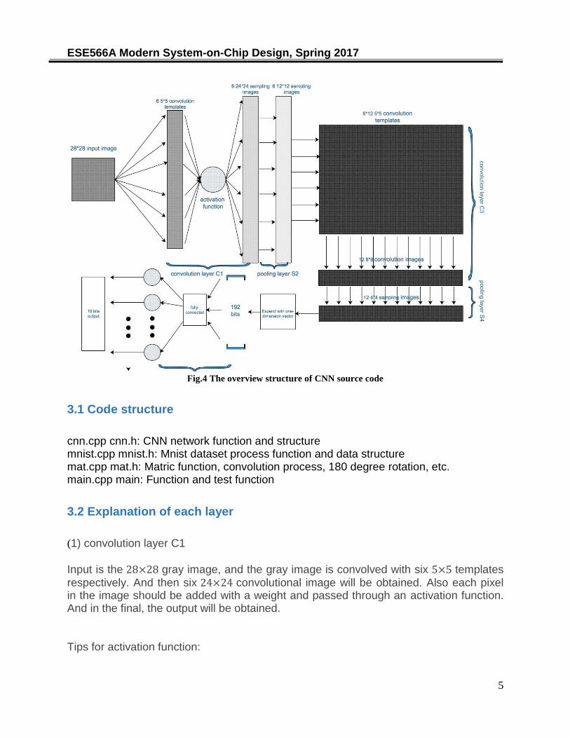
This convolutional network has five layers. The main structures contain convolution layer,

pooling layer, convolution layer, pooling layer and fully connected single-layer neural layer

(output layer), as Fig.4 shows.

ESE566A Modern System-on-Chip Design, Spring 2017

5

Fig.4 The overview structure of CNN source code

3.1 Code structure

cnn.cpp cnn.h: CNN network function and structure mnist.cpp mnist.h: Mnist dataset process function and data structure mat.cpp mat.h: Matric function, convolution process, 180 degree rotation, etc. main.cpp main: Function and test function

3.2 Explanation of each layer

(1) convolution layer C1

Input is the 28×28 gray image, and the gray image is convolved with six 5×5 templates

respectively. And then six 24×24 convolutional image will be obtained. Also each pixel in the image should be added with a weight and passed through an activation function. And in the final, the output will be obtained. Tips for activation function:

ESE566A Modern System-on-Chip Design, Spring 2017

6

Fig.5 Sigmoid and Tanh function diagram

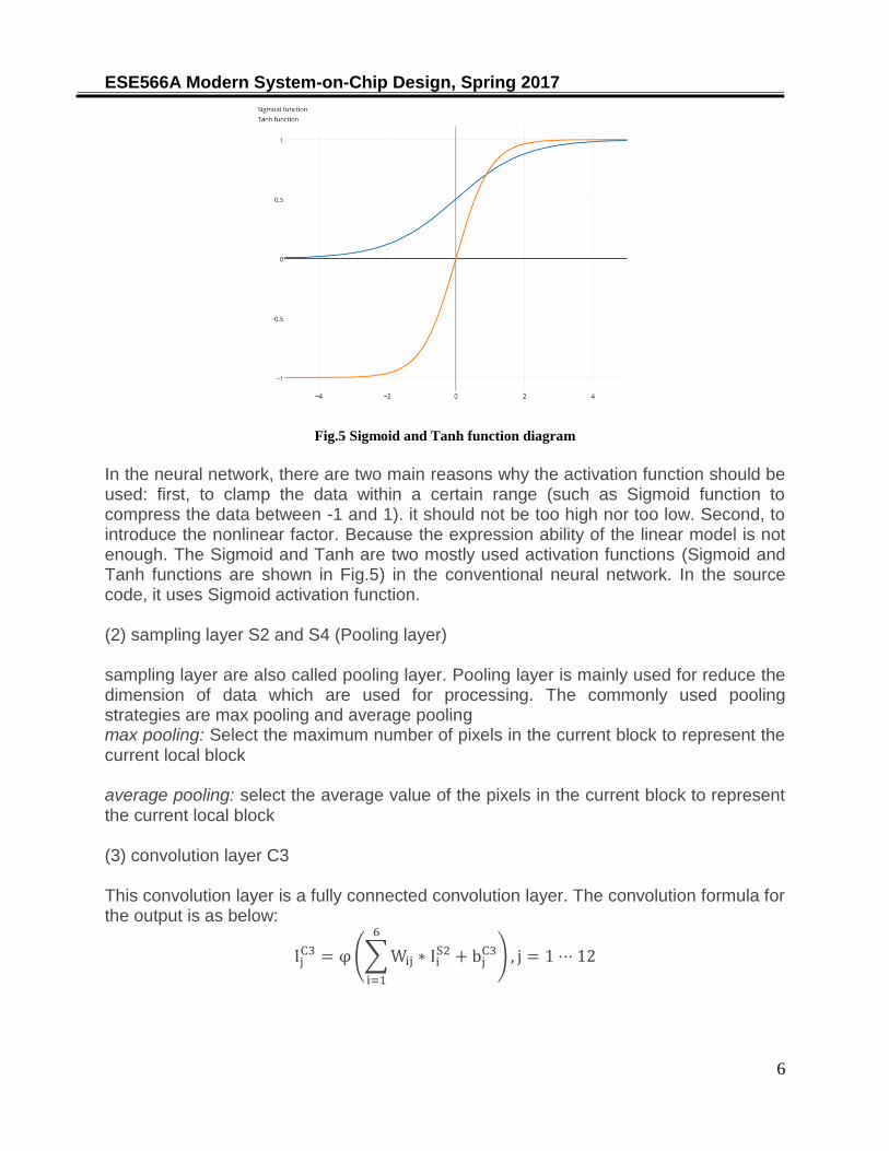
In the neural network, there are two main reasons why the activation function should be used: first, to clamp the data within a certain range (such as Sigmoid function to compress the data between -1 and 1). it should not be too high nor too low. Second, to introduce the nonlinear factor. Because the expression ability of the linear model is not enough. The Sigmoid and Tanh are two mostly used activation functions (Sigmoid and Tanh functions are shown in Fig.5) in the conventional neural network. In the source code, it uses Sigmoid activation function. (2) sampling layer S2 and S4 (Pooling layer) sampling layer are also called pooling layer. Pooling layer is mainly used for reduce the dimension of data which are used for processing. The commonly used pooling strategies are max pooling and average pooling max pooling: Select the maximum number of pixels in the current block to represent the current local block average pooling: select the average value of the pixels in the current block to represent the current local block (3) convolution layer C3 This convolution layer is a fully connected convolution layer. The convolution formula for the output is as below:

IjC3 = φ (∑ Wij

6

i=1

∗ IiS2 + bj

C3) , j = 1 ⋅⋅⋅ 12

ESE566A Modern System-on-Chip Design, Spring 2017

7

I represents the image, W represents the convolution template, b represents bias, φ represents the activation function, i represents the input image order number (i = 1 ∼ 6), and j represents the output image order number (j = 1 ∼ 6)

In the convolution layer C3, it can be seen that the inputs are 6 12×12 image, and the outputs are 12 8×8 image. The required training parameters are 72 5×5 convolution templates w and 12 bias b (each bias associated with each template is same) (4) Output layer O5:

Go through the pooling layer S4, 12 4×4 image will be obtained. Expand all the images input one dimension, we will get a vector of 12×4×4 = 192 bits. The output layer is composed of 192 bits input and 10 bits fully connected single-layer neural network. It contains 10 neurons, and each neuron are connected with 192 bits input, which means each neuron has 192 bits input and 1 bit output. The processing formula is shown as below:

IjO5 = φ (∑ Wij

192

i=1

∗ Ii + bjO5) , j = 1 ⋅⋅⋅ 10

j represents the order number of output neuron, and I represents the order number of input.

Therefore, in this layer, there are 192×10 weight w, and 10 bias b.

3.3 Forward propagation process

The forward propagation process actually refers to input image data and get the output. Here we will introduce the convolution layer C1 (or C3) forward propagation process (S2, S4 and O5 layers are omitted because the process of them are quite strait-forward). The convolution layer C1 (or C3) has 6 convolution templates. Each template has 6 outputs for 1 input, which means it will have 6 output. The image convolution formula is shown below:

g(x, y) = ∑ ∑ w(s, t) ∙ f (x − s −(c − 1)

2, y − t −

(r − 1)

2) , c, r = 2k + 1

r

t=0

c

s=0

3.4 Error back propagation process

The error back propagation method is the basis of neural network learning. Actually it is the process that use the gradient descent method to compute the weight of minimum error.

ESE566A Modern System-on-Chip Design, Spring 2017

8

The updating formula of gradient descent method is shown as below:

Wn+1 = Wn − ∆Wn

∆Wn = η∂Ee

n

∂Wn= η

∂Een

∂un

∂un

∂Wn= ηδnXn

un = WnXn

δn =∂Ee

n

∂un

Here, W represents weight, E represents the error energy, n represents nth iteration, η

represents the learning rate, Y represents output, and δ represents the local gradient. Backward propagation datapath is used for CNN training. However, in this project, you don’t need to implement backward propagation datapath in the CNN hardware accelerator design. Because the main functionality for this design is to do the handwriting dataset classification which actually is the CNN test part not training part. If you are interested in the entire picture of this CNN code including the backward propagation. You can read the Appendix A ‘The analysis of the back propagation process in this CNN code’.

3.5 Matlab reference resource

This referenced C/C++ code provided in github is the C/C++ implementation of DeepLearningToolBox (Matlab), if you want to learning this CNN work in deep, such as analyzing the intermediate results of each layer, you can download DeepLearningToolBox in following website and have fun with it.

https://github.com/rasmusbergpalm/DeepLearnToolbox

4. Possible optimizations using parallelism in referenced C/C++ code

A vast amount of the computation required by a CNN can be parallelized. Thus, in order

to achieve the processing of the network it is important that these potential parallelisms

are identified and exploited. The most obvious being:

1. The convolution of a matrix n×n using a k×k kernel consists of (n − k + 1) × (n − k +1) convolution operation, which each can be done in parallel. Thus convoluting the

whole matrix could potentially take only the time it takes to perform one convolution

operation.

ESE566A Modern System-on-Chip Design, Spring 2017

9

2. The subsampling/pooling operation can also be parallelized by pooling all of the

individual sub-matrices at the same time.

3. The computation of each of the individual feature maps and their corresponding

subsampling/pooling.

4. It is also possible to parallelize the computation of the feature maps that take more

than one matrix as input. This is the case in the subsequent layers after the first.

5. The activation of each neuron in the fully connected layer. One option is to parallelize

them by creating a binary tree multiplier, where you have n units compute the product of

the input and its respective weight, then you use 𝑛

2 units to add two of the results each,

and so on until you have a single value. This will reduce the time it takes from n time to

log2 𝑛 time if they can all be done in parallel.

5. How to get started

You are expected to accept the lab assignment in the link by click the button “Accept this assignment”.

https://classroom.github.com/group-assignment-invitations/7b25eac1efb20a7871dbc074ea73befc

If you are the first time to use github, you should generate your own public key and add it to your github account, or you will have permission denied when you git clone the repository form our github classroom. When you add the ssh public key, you can follow the link below:

https://help.github.com/articles/connecting-to-github-with-ssh/

And then create a folder in your own linux server account and git clone your lab assignment repository. There are the command lines you may refer below:

% mkdir name_folder

% cd name_folder

% git clone git@github.com:wustl-ese566/class-project-team#.git

% cd class-project-team# / (i.e., cd class-project-team1/)

This repository class-project-team#/ contains three folders:

• CNN_Referenced_Code/CNN: a folder that contains the C/C++ source code of

CNN design

• CNN_Referenced_Code/Mnist: a folder that contains the MNIST handwriting

dataset

• CNN_Accelerator: a folder contains that testbench, and your own Verilog code

should be in this folder

ESE566A Modern System-on-Chip Design, Spring 2017

10

CNN_Referenced_Code/CNN folder have 8 files:

• cnn.cpp: each layer definition and training, test function and etc.

• cnn.h: variables of each layer in this CNN and function claim

• mnist.cpp: Mnist dataset image and label read function

• mnist.h: variables of Mnist dataset image and function claim

• mat.cpp Matric computation, convolution computation, 180 degree rotation, max computation and summation etc.

• mat.h: variables definition and function claim of mat.cpp

• main.cpp main: training function and test function

• Minst.bin: 16bits fixed point weight matrix dataset

CNN_Referenced_Code/Mnist folder have 4 files, these 4 files are downloaded from Mnist handwriting dataset.

CNN_Accelerator folder have 1 file:

• CNN_tb.v: this is an incompleted testbench, it will provide the interface for feeding in 28 × 28 test image and weight matrix

Please be sure to source the class setup script using the following command before

compiling your source code: module add ese461.

6. Required Project Deliverables

6.1 Basic functionality

Refer to CNN C/C++ code and paper to build your own CNN hardware accelerator. Your CNN hardware accelerator design should achieve the forward propagation function of CNN to accomplish the handwriting dataset classification.

For the CNN functionality evaluation, we will randomly feed in a 28 × 28 handwriting image and the accelerator your team have built should compute the right classification of the image which is fed in. (Don’t worry about correct prediction rate. We will use a 100% predictable image we have tested to evaluate your work) Note: we will provide a 16 bits fixed point weight matrix which contains C1, C3 and O5 weight values.

6.2 Performance expectation

ESE566A Modern System-on-Chip Design, Spring 2017

11

Although there is no specific performance targets in the project as long as you are able to demonstrate the basic functionality (as discussed in Section 6.1), it is important to demonstrate the “selling point” of your design, be it low latency, high throughput, low power, or small area. You want to be able to demonstrate significant design efforts and techniques in your project to optimize for one or more performance specifications. You can refer to the paper we reviewed in class (DianNao and Eyeriss) and the optimization techniques suggested in Section 4 for inspiration for key feature of your accelerator design such as pipelining, matrix tiling, or other datapath optimization. You should organize your project presentation and report to highlight the design features in your hardware accelerator, as if you are writing a reference paper and giving a conference presentation to showcase your design with compelling results and rigorous analysis. To report credible speed, power, and area numbers, you need to go through all the steps you did in lab1:

• Use Synopsys VCS to compile the Verilog source code of CNN hardware accelerator

• Use Design Compiler to do the synthesis of CNN hardware accelerator

• Use Cadence Encounter to do the place and route of CNN hardware accelerator

To evaluate your design, we need all the source Verilog codes, the test bench, and all the Tcl design script you use for synthesis and place-and-route. We will re-run the simulation with randomly chosen test image and check the classification output. We will also review your code to verify the claimed design features. Each feature will point that contribute to your final grades. Also we will simulate your design at the clock frequency specified in your report and verify its error-free operation. We will look at the waveform analysis and all synthesis reports of your design. Teams that are able to achieve the best specification in the class (fastest execution time, lowest power consumption, or smallest silicon area) will get extra bonus points.

6.3 Report expectation

Each team should turn in a well-organized detailed report to explain your work. In the report, you should show the implementation details and datapath optimization method and analysis featured in your accelerator design. In the appendix, you should include screen shots of critical waveform and synthesis reports and give explanations of them, as well as screen shots of the final physical layout after place-and-route. In the end, you should paste your code and provide detailed comments for your code.

ESE566A Modern System-on-Chip Design, Spring 2017

12

7. Project submission

Please submit your lab assignment on Github. You are expected to submit your report,

all hardware design module files, and class_project_dc.tcl fill. If you modify the test

benches or create new ones, submit them too.

To submit your job, execute the following command:

(Note: the first two commands just need to be done once for the entire semester.)

% git config --global user.name “your_user_name”

% git config --global user.email “your_email_for_github”

% cd directory_of_your_lab_assignment/class-project-team#/

% git add CNN_Accelerator/all module Verilog file

% git add CNN_Accelerator/class_project_dc.tcl

% git add class-project-team#-report.pdf

% git commit -m “your commits”

% git push -u origin master

You also should submit anything else you think may help us understand your code and

result.

Please do not submit files like compiling result(simv) or simulation data(.vpd).

8. Acknowledgement

[1] https://algobeans.com/2016/01/26/introduction-to-convolutional-neural-network/

[2] http://yann.lecun.com/exdb/mnist/

[3] https://daim.idi.ntnu.no/masteroppgaver/013/13656/masteroppgave.pdf

ESE566A Modern System-on-Chip Design, Spring 2017

13

Appendix A

The analysis of the back propagation process in this CNN code (1) Output layer (single-layer neural network) error is defined as the difference between actual output and expected output.

Een =

1

2∑(di − yi)

2

N

i

Here, d represents the expected output, y represents actual output, i represents the output bit. In this network, the output is 10 bits. Therefore, N = 10. The derivative of error energy with respect to weight:

∂EeO5

∂WijO5

=∂Ee

O5

∂yjO5

∙∂yj

O5

∂ujO5

∙∂uj

O5

∂wijO5

ujO5 = ∑ Wij

O5yiS4 +

192

i

bjO5

yjO5 = φ(uj

O5)

EeO5 =

1

2∑(di − yj

O5)2

N

i

∂EeO5

∂WijO5

= −1 ∙ φ̃(ujO5) ∙ yi

S4

ESE566A Modern System-on-Chip Design, Spring 2017

14

∂EeO5

∂bjO5

= −1 ∙ φ̃(ujO5) ∙ 1

In this source code, it uses Sigmoid activation function, so the derivative is:

φ̃(ujO5) = yi

O5 ∙ (1 − yiO5)

The local gradient is:

δiO5 =

∂EeiO5

∂uiO5

=∂Eei

O5

∂yiO5

∙∂yi

O5

∂uiO5

= −1 ∙ φ̃(ujO5)

(2) The output layer which is followed by the pooling layer S4 Since there is no weight in this layer, we don’t need to update weight. But we need to pass the error energy to the next layer. Therefore, we have to compute the local

gradient δ. The definition of this is shown as below:

δiS4 =

∂EeS4

∂ujS4

Here, j indicates the pixel’s order number of output image. There are 12×4×4 = 192 output pixels in S4, so j = 1 ∼ 192.

And the local gradient δ of output layer O5 is computed already:

δiS4 =

∂EeS4

∂ujS4 =

∂EejS4

∂yjS4 ∙

∂yjS4

∂ujS4 δi

O5 =∂Eei

O5

∂uiO5 =

∂EeiO5

∂yiO5 ∙

∂yjO5

∂uiO5 = −1 ∙ φ̃(uj

O5)

EejS4 = ∑ Eeij

O510i uj

O5 = ∑ WjiO5yj

S4 +192j bi

O5

δjS4 =

∂EejS4

∂yjS4 ∙

∂yjS4

∂ujS4 = ∑

∂EeiO5

∂uiO5

10i ∙

∂uiO5

∂yjS4 ∙

∂yjS4

∂uJS4 = φ̃(uj

S4) ∑ δiO5 ∙10

i WjiO5

Since pooling layer does not have activation function, therefore, the derivative of φ is 1. Then,

δjS4 = ∑ δi

O5 ∙

10

i

WjiO5

From the above formula, we could compute the local gradient δ which pass from output layer O5 to pooling layer S4. We can see that the local gradient δ value passed to the output pixel j of the pooling layer is actually the sum of the weights corresponding to the

local gradient δ value of the following layer output.

ESE566A Modern System-on-Chip Design, Spring 2017

15

(3) convolution layer C1, C3 which connected the following pooling layer In order to compute the parameters, the output of S4 and O5 layers are expanded to one-dimension vector. Therefore, all pixels could be labeled with i and j. And we use m(x,y) to indicate the coordinate of the pixel in the mth output template. The local

gradient δ is defined as:

δm(x,y)C3 =

∂EeC3

∂um(x,y)C3

=∂Eem(x,y)

C3

∂ym(x,y)C3

∙∂ym(x,y)

C3

∂um(x,y)C3

The error energy delivered to the pixel is equal to the sum of the pixel error energy

associated with this pixel. Here, i indicates all pixels in sampling neighborhood Θ of m(x,y).

Eem(x,y)C3 = ∑ Eei

S4

iϵϑm(x,y)

Since we use average pooling method, the output of S4 is the average of all pixels in the neighborhood of current pixel. Here, S indicates the number of the pixels in the

neighborhood Θ. In this code we use 2×2 sampling block, therefore, S=4.

uiS4 =

1

S∑ ym(x,y)

C3

m(x,y)ϵϑ

therefore, the gradient delivered from S4 to C3 is:

δm(x,y)C3 = ∑

∂EeiS4

∂ym(x,y)C3

iϵϑm(x,y)

∙∂ym(x,y)

C3

∂um(x,y)C3

= ∑∂Eei

S4

∂uiS4

iϵϑm(x,y)

∙∂ui

S4

∂ym(x,y)C3

∙∂ym(x,y)

C3

∂um(x,y)C3

=1

S∑ 𝛿i

S4

iϵϑm(x,y)

∙ φ̃(um(x,y)C3 )

Next we update weight in C3 layer using the local gradient δ:

C3 layer totally has 6×12 = 70 5×5 templates. First, we define n = 1 ∼ 6, m = 1 ∼ 12 indicates the label of templates. s, t indicates the position of parameter in this template.

um(x,y)C3 = ∑ ∑ ∑ Wnm(s,t)

C3

r

t=0

c

s=0

N

n

∙ yn(x−s−

(c−1)2

,y−t−(r−1)

2)

S2

ESE566A Modern System-on-Chip Design, Spring 2017

16

∂EeC3

∂Wnm(s,t)C3

= ∑ ∑ ∑∂Ee

C3

∂um(x,y)C3

∙

h

y=0

w

x=0

M

m

∂um(x,y)C3

∂Wnm(x,y)C3

= ∑ ∑ ∑ δm(x,y)C3 ∙

h

y=0

w

x=0

M

m

yn(x−s−

(c−1)2

,y−t−(r−1)

2)

S2

∂EeC3

∂WnmC3

= ∑ correlation(δmC3, yn

S2) =

M

m

∑ conv(δmC3, rotate180(yn

S2))

M

m

∂EeC3

∂bmC3

= ∑ ∑ δm(x,y)C3

h

y=0

w

x=0

Similarly, we can get weight updating formula of C1 layer. Here M=6, N=1, and y indicates the input image.

δm(x,y)C1 = ∑

∂EeiS2

∂ym(x,y)C1

iϵϑm(x,y)

∙∂ym(x,y)

C1

∂um(x,y)C1

= ∑∂Eei

S2

∂uiS2

iϵϑm(x,y)

∙∂ui

S2

∂ym(x,y)C3

∙∂ym(x,y)

C3

∂um(x,y)C3

=1

S∑ δi

S2

iϵϑm(x,y)

∙ φ̃(um(x,y)C1 )

um(x,y)C1 = ∑ ∑ ∑ Wnm(s,t)

C1

r

t=0

c

s=0

N

n

∙ yn(x−s−

(c−1)2

,y−t−(r−1)

2)

l

∂EeC1

∂Wnm(s,t)C1

= ∑ ∑ ∑∂Ee

C1

∂um(x,y)C1

∙

h

y=0

w

x=0

M

m

∂um(x,y)C1

∂Wnm(x,y)C1

= ∑ ∑ ∑ δm(x,y)C1 ∙

h

y=0

w

x=0

M

m

yn(x−s−

(c−1)2

,y−t−(r−1)

2)

l

∂EeC1

∂WnmC1

= ∑ correlation(δmC1, yn

l ) =

M

m

∑ conv(δmC1, rotate180(yn

l ))

M

m

∂EeC1

∂bmC1

= ∑ ∑ δm(x,y)C1

h

y=0

w

x=0

(4) Pooling layer S2 which connected following convolution layer

Here, n indicates the order number (n = 1 ∼ 6) of output image of current S2 layer, and m indicates the order number (m = 1 ∼ 12) of output image of current C3 layer.

δn(x,y)S2 =

∂EeS2

∂um(x,y)S2

=∂Een(x,y)

S2

∂yn(x,y)S2

∙∂yn(x,y)

S2

∂un(x,y)S2

ESE566A Modern System-on-Chip Design, Spring 2017

17

Een(x,y)S2 = ∑ ∑ ∑ E

em(x−s−(c−1)

2,y−t−

(r−1)2

)

C3

r

t=0

c

s=0

M

m

δn(x,y)S2 = ∑ ∑ ∑

∂Eem(x−s−

(c−1)2

,y−t−(r−1)

2)

C3

∂ym(x,y)S2

r

t=0

c

s=0

M

m

∙∂ym(x,y)

S2

∂um(x,y)S2

δn(x,y)S2 = ∑ ∑ ∑

∂Eem(x−s−

(c−1)2

,y−t−(r−1)

2)

C3

∂um(x−s−

(c−1)2

,y−t−(r−1)

2)

C3

r

t=0

c

s=0

M

m

∙

∂um(x−s−

(c−1)2

,y−t−(r−1)

2)

C3

∂yn(x,y)S2

∙∂yn(x,y)

S2

∂yn(x,y)S2

um(x,y)C3 = ∑ ∑ Wnm(s,t)

C3 ∙ yn(x−s−

(c−1)2

,y−t−(r−1)

2)

S2

r

t=0

c

s=0

δn(x,y)S2 = ∑ ∑ ∑ δ

m(x−s−(c−1)

2,y−t−

(r−1)2

)

C3 ∙

r

t=0

c

s=0

M

m

Wn,m(s,t)C3 ∙

∂ym(x,y)S2

∂um(x,y)S2

Therefore, the local gradient δ of nth image is:

𝛿𝑛𝑆2 = ∑ 𝑐𝑜𝑟𝑟𝑒𝑙𝑎𝑡i𝑜𝑛(𝛿𝑚

𝐶3, 𝑊𝑛𝑚𝐶3)

𝑀

𝑚