ECE 5650/4650 Python Project 1 This project is to be treated as a take-home exam, meaning each student is to due his/her ownwork. The exception to this honor code is for ECE 4650 students I will allow you to work in teamsof two if desired. Still, teams do not talk to other teams. The project due date is no later than 5:00PM Tuesday, November 26 Dec. 3, 2019 (after Thanksgiving week). Getting it completed earlieris recommended. To work the project you will need access to Jupyter Notebook. All the neededfunctions can be found in numpy, the signal module of scipy and scikit-dsp-comm. found in theproject ZIP package set1p.zip.

IntroductionIn this project you are introduced to using Python’s Scipy Stack, which is a collection of Pythonpackages for doing engineering and scientific computing. The core portion of the SciPy stack isknown as PyLab, which imports the numpy and matplotlib. This Python DSP project will get youacquainted with portions of the Python language and PyLab and then move into the exploration of

• LCCDEs with non-zero initial conditions

• Multi-rate sampling theory

• Polyphase rate changing class

• Studying an IIR notch filter

• PyAudio_helper real-time DSP apps (LinearChirp, speech with noise and tone jamming)

It is the student’s responsibility to learn the very basics of Python from one of the various tutorialson the Internet, such as Python Basics (see the link below).

Python Basics with NumPy and SciPyTo get up and running with Python, or more specifically the PyLab (numpy and matplotlib loadedinto the environment) for engineering and scientific computing, please read through the tutorial Ihave written in an Jupyter notebook. The PDF version of the notebook can be found at http://www.eas.uccs.edu/wickert/ece5650/notes/PythonBasics.pdf.

Problems

Causal Difference Equation Solver with Non-Zero Initial Conditions1. In this problem you gain some experience in Python coding by writing a causal difference

equation solver. You will actually be writing a Python function (def) that you will input fil-ter coefficients and , the input signal , and initial condi-

tions, and , to then obtain the output, . The starting point is

b0 b1 1 a1 a2 x n

xi yi y n

Introduction 1

ECE 5650/4650 Python Project 1

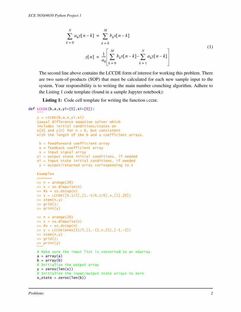
(1)

The second line above contains the LCCDE form of interest for working this problem. Thereare two sum-of-products (SOP) that must be calculated for each new sample input to thesystem. Your responsibility is to writing the main number crunching algorithm. Adhere tothe Listing 1 code template (found in a sample Jupyter notebook):

Listing 1: Code cell template for writing the function LCCDE.

def LCCDE(b,a,x,yi=[0],xi=[0]): """ y = LCCDE(b,a,x,yi,xi) Causal difference equation solver which includes initial conditions/states on x[n] and y[n] for n < 0, but consistent with the length of the b and a coefficient arrays. b = feedforward coefficient array a = feedback coefficient array x = input signal array yi = output state initial conditions, if needed xi = input state initial conditions, if needed y = output/returned array corresponding to x Examples ======= >> n = arange(20) >> x = ss.dimpulse(n) >> #x = ss.dstep(n) >> y = LCCDE([0,1/3],[1,-5/6,1/6],x,[1],[0]) >> stem(n,y) >> grid(); >> print(y) >> n = arange(20) >> x = ss.dimpulse(n) >> #x = ss.dstep(n) >> y = LCCDE(ones(5)/5,[1,-1],x,[5],[-1,-1]) >> stem(n,y) >> grid(); >> print(y) """ # Make sure the input list is converted to an ndarray a = array(a) b = array(b) # Initialize the output array y = zeros(len(x)) # Initialize the input/output state arrays to zero x_state = zeros(len(b))

aky n k– k 0=

N

bkx n k–

k 0=

M

=

y n 1a0----- bkx n k–

k 0=

M

aky n k– k 1=

N

–=

Problems 2

ECE 5650/4650 Python Project 1

y_state = zeros(len(a)-1) # Load the input initial conditions into the # input/output state arrays if len(a) > 1: for k in range(min(len(yi),len(a)-1)): y_state[k] = yi[k] if len(b) > 1: for k in range(min(len(xi),len(b)-1)): x_state[k+1] = xi[k]

# Process sample-by-sample in a loop

return y

In writing the main loop code consider how x_state and y_state are used:

To update the state arrays on each loop iteration consider using the Numpy functions roll()and sum() for ndarrays.

a) Complete the function LCCDE(). Feel free to do all of your code development right insidean Jupyter notebook.

b) Test the code with the two examples given in the doc string of the code template. Theprinted listing of output values needs to be included in your report for grading purposes.Feel free to validate your code by hand calculations or other means you can devise.

c) Compare the execution speed LCCDE() with signal.lfilter() under zero initial condi-tions using the IPython magic $timeit. An example of the setup for LCCDE() is shownbelow:

Code To Write

x n x n 1– x n M– x n 2– x_state

y n 1– y n 2– y n N– y n 3– y_state

Product with b coefficient array

Product with a coefficient array

Problems 3

ECE 5650/4650 Python Project 1

Multirate Systems with Python Using PyLab

2. In this first task you will do some basic signals and systems problem solving using PyLabwith SciPy and functions in sigsys.py and signal.find_peaks Note: In Task 1 I will beguiding you step-by-step. In the remaining tasks things become more open-ended.

a) Generate 10,000 samples of . The large number of samples insures a high resolu-tion spectral estimate.

b) Plot for using plot(x,y). Label your axis accordingly.

c) Plot the power spectrum of using

f,Sx = ss.simple_SA(x, NS, NFFT, fs, window='hanning')

with NS=NFFT=2048. Then plot in dB, that is plot . Note: Here the powerspectrum as defined in notes Chapter 4, , is related to with additional scaling and averaging. Also, setting fs=1 means the frequency axis arrayf corresponds to , which convenient for the present analysis.

d) Next verify that the PSD spectral peaks are where you expect based on theory. Tonumerically find the peaks use the scipy.signal function index=detect_peaks(Sx), asshown in Listing 2.

Listing 2: Code snippet for listing the peaks found by simple.SA.

n = arange(10000)x = cos(2*pi*n/20) + 3*cos(2*pi*n/5)

f,Sx = ss.simple_SA(x,2048,2048,1,window='hanning')plot(f,10*log10(Sx))grid();xlabel(r'Normalized Frequency $\omega/(2\pi)$')ylim([-30,0])ylabel(r'Power Spectrum $P_{x}(\omega)$ (dB)');

# argument height = -15 sets the detection threshold at -15 dB idx_peaks,pk_prop = signal.find_peaks(10*log10(Sx),height=-15)for k in idx_peaks:

print('Spectrum peak of {:4.2f} Hz at {:8.4f}dB.'\ .format(f[k],10*log10(Sx[k])))

Figure 1: Downsampler/upsampler with lowpass interpolation filter blockdiagram.

b=firwin()Lowpass65 Taps

fc

x n y n 4 4

z1 n z2 n

310------n cos 2

3---n cos+=

x n

x n 0 n 50

x n

10log10 Sx Pxx Pxx 2f = X e

j 2

2

Problems 4

ECE 5650/4650 Python Project 1

Spectrum peak of 0.05 Hz at -12.9502 dB.Spectrum peak of 0.20 Hz at -3.4078 dB.

Note: In the above code snippet, the \ is Python’s line continuation character. It is possi-ble to break lines on , (commas) too.

e) Using z1 = ss.downsample(x,M) produce and repeat parts (b) – (d) for z1. Youneed to compare the experimental results for the spectral frequency locations with the-ory. The amplitude values are not a concern at this point. The fact that you generatedsinusoids at two different amplitudes should help you keep track of which frquency iswhich, in spite of any aliasing that may be present.

f) Using z2 = ss.upsample(z1,L) produce and repeat parts (b) – (d) for z2. As aresult of the upsampling, modify the plot range from part (b) to .

g) Design the lowpass interpolation filter as indicated in the block diagram. Choose the cut-off frequency accordingly. The firwin function is in the SciPy signal module:

b = signal.firwin(numtaps, cutoff)

where here numtaps=65 and cutoff=2*fc/fs, where and the samplingrate at this point. Plot the frequency response magnitude and phase of this filter.Also obtain a pole-zero plot. The relevant Python functions are shown in Listing 3.

Listing 3: Plotting frequency response from the ground up and also plotting apole-zero plot.

f = arange(0,0.5,.001)

w,H = signal.freqz(b,1,2*pi*f)

plot(f,20*log10(abs(H)))

grid();

xlabel(r'Normalized Frequency $\omega/(2\pi)$')

ylabel(r' Magnitude Response $|H(e^{j\omega})|$ (dB)');

figure()

plot(f,angle(H))

grid();

xlabel(r'Normalized Frequency $\omega/(2\pi)$')

ylabel(r' Phase Response $\angle H(e^{j\omega})$ (rad)');

ss.zplane(b,[1],False,1.5) #Turn off autoscale if a bad root appears

h) Finally, process through the lowpass interpolation filter to produce . The rel-evant Python function to perform filtering is:

y = signal.lfilter(b,a,x)

where for an FIR filter a=1. With y in hand, repeat parts (b) – (d). To compensate for theFIR filter delay, in part (b) change the plot range to . Comment on yourfinal results. Note: Your lowpass filter will push the amplitudes of the upsamplingimages down, but the find_peaks function will still find them. The argument height=can be used to ignore peaks below the height threshold.

z1 n

z2 n 0 n 100

fc c 2 =fs 1=

z2 n y n

50 n 100

Problems 5

ECE 5650/4650 Python Project 1

Polyphase Decimator Investigation

3. In this problem you will implement a decimator in one of two forms using Python’s numpypackage to take advantage of vectorizing. In part (a) you will implement the decimator asthe serial processing block composed of an FIR lowpass filter followed by a down samplerblock. In part (b) you will implement the decimator using polyphase filtering. The mainpoint of the problem is to see that both approaches yield identical waveform outputs. Thetest input signal is an analog waveform composed of two sinusoids:

(2)

which enters the decimator input at a sampling rate of Msps. The decimation factoris , so the output sampling rate is Msps. Create 200 samples of this wave-form for testing the two implementations. An approach for generating this test vector isshown in Listing 4.

Listing 4: Test vector generation approach using the function x_vec().

def x_vec(N_samp, fs = 20e6, f1 = 1e6, f2 = 3.5e6): """ Simple test vector generator Parameters ---------- N_samp : number samples to generate fs : the sampling rate in Hz f1 : frequency one f2 : frequency two """ n = arange(N_samp) x = 5*cos(2*pi*f1*n/fs) + 2*cos(2*pi*f2*n/fs)

return n, x

a) Complete a reference design that implements the design of Figure 2 using signal.lfil-ter() and ss.downsample(). Yes, you will be throwing away samples with thisapproach. To obtain the FIR filter coefficients use the approach of Listing 5. The filter

order is low because with Df1 = 0.2 the desired transition bands runs from 0.8 to 1.2 of or . For this problem the transition width is OK, but you may want to

experiment on your own with smaller values, e.g. Df2 = 0.15 or smaller. Make sure youuse the same design for both parts (a) and (b). Finally, test the design using N_samp = 200samples of the waveform given in (2) and in code via Listing 4.

xa t 5 2 106t 2 2 3.25

610 t cos+cos u t =

fs 20=M 5= fs out 4=

M 1–

FIR Lowpass

c M=

Mx n z n b array holds FIRcoefficients

y n

Keep every Mth sample

Figure 2: A decimate by M system implemented as a cascade of a lowpass anda downsampler.

H z

c 20% 20%

Problems 6

ECE 5650/4650 Python Project 1

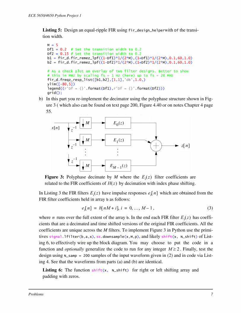
Listing 5: Design an equal-ripple FIR using fir_design_helperwith Df the transi-tion width.

M = 5Df1 = 0.2 # Set the transition width to 0.2Df2 = 0.15 # Set the transition width to 0.2b1 = fir_d.fir_remez_lpf((1-Df1)*1/(2*M),(1+Df1)*1/(2*M),0.1,60,1.0)b2 = fir_d.fir_remez_lpf((1-Df2)*1/(2*M),(1+Df2)*1/(2*M),0.1,60,1.0)

# As a check plot an overlay of two filter designs. Better to show # this in MHz by scaling fs = 1 Hz (here) up to fs = 20 MHzfir_d.freqz_resp_list([b1,b2],[1,1],'dB',1.0,)ylim([-80,5])legend((r'Df = {}'.format(Df1),r'Df = {}'.format(Df2)))grid();

b) In this part you re-implement the decimator using the polyphase structure shown in Fig-ure 3 ( which also can be found on text page 200, Figure 4.40 or on notes Chapter 4 page55.

In Listing 3 the FIR filters have impulse responses which are obtained from theFIR filter coefficients held in array b as follows:

, (3)

where runs over the full extent of the array b. In the end each FIR filter has coeffi-cients that are a decimated and time shifted versions of the original FIR coefficients. All thecoefficients are unique across the M filters. To implement Figure 3 in Python use the primi-tives signal.lfilter(b,a,x), ss.downsample(x,M,p), and likely shift(x, N_shift) of List-ing 6, to effectively wire up the block diagram. You may choose to put the code in afunction and optionally generalize the code to run for any integer . Finally, test thedesign using N_samp = 200 samples of the input waveform given in (2) and in code via List-ing 4. See that the waveforms from parts (a) and (b) are identical.

Listing 6: The function shift(x, N_shift) for right or left shifting array andpadding with zeros.

E0 z( )

E1 z( )

EM 1– z( )

. . .

x n[ ]

w n[ ]

z1–

z1–

z1–

M

M

M

. . .

pp y t e o sa p g de t ty

Figure 3: Polyphase decimate by M where the filter coefficients arerelated to the FIR coefficients of by decimation with index phase shifting.

Ei z H z

z n

Ei z ei n

ei n b nM i+ i 0 M 1–= =

n Ei z

M 2

Problems 7

ECE 5650/4650 Python Project 1

def shift(x, N_shift): """ Right or left shift an array filling with zeros. Note: numpy roll wraps the shifted values """ x_shift = np.empty_like(x) if N_shift >= 0: x_shift[:N_shift] = 0 x_shift[N_shift:] = x[:-N_shift] else:

x_shift[N_shift:] = 0 x_shift[:N_shift] = x[-N_shift:]

return x_shift

c) Finally, compare execution time between the two implementations using

the cell magic (%%timeit for a whole cell) or the line magic (%timeit at the start of a line)capability of the Jupyter notebook. A line magic for the function wrapping the part (a)decimator yields:

on my 2.5 year old Dell Precision 5520 laptop.

Difference Equations, Frequency Response, and Filtering

4. In this problem we consider the steady-state response of an IIR notch filter. To begin withwe know that when a sinusoidal signal of the form

(4)

is passed through an LTI system having frequency response , the system outputis of the form

(5)

In this problem the input will be of the form , so the outputwill consist of both the transient and steady-state responses. For n large the output is insteady-state, and we should be able to determine the magnitude and phase response at from the waveform. The filter of interest is

(6)

where controls the center frequency of the notch and controls the bandwidth.

a) Using signal.freqz() plot the magnitude and phase response of the notch for and . Plot the magnitude response as both a linear plot, ,

and in dB, i.e., .

x n A 0n + cos= – n

H ej

y n A H ej0 0n + H ej0 + cos= – n

x n A 0n + u n cos=

0

H ej 1 2 0 e j–cos e j2–+–

1 2r 0 e j–cos r2ej2–

+–---------------------------------------------------------------------=

0 r

0 2= r 0.9= H ej 20log10 H ej

Problems 8

ECE 5650/4650 Python Project 1

b) Using signal.lfilter() , input for . Determine from the outputsequence plot approximate values for the filter gain and phase shift at . To dothis you look at the change in amplitude and the change in zero crossing location. Notethat the filter still has center frequency . Also, plot the transient response as aseparate plot by subtracting the known steady-state response from the total response. Todo this note your simulation gives you the total response, so to get to just the transientyou have to subtract the known from theory steady-state response from the totalresponse.

c) Assume that the filter operates within an A/D- -D/A system. An interfering signalis present at 120 Hz and the system sampling rate is set at 2000 Hz. Determine sothat the filter removes the 120 Hz signal. Simulate this system by plotting the filter out-put in response to the interference signal input. Determine in ms, how long it takes forthe filter output to settle to , assuming the input amplitude is one.

Real-Time DSP Using pyaudio_helper

5. In this problem you will process a speech files in real-time using the scikit-dsp-comm mod-ule pyaudio_helper. Two important references to get started with pyaudio_helper are theScipy 2018 paper [4] and ECE 4680 lab materials also on the ECE 5650 Web Site. WithPyAudio and the use of the pyaudio_helper module, a DSP algorithm developer can imple-ment frame-based real-time DSP as depicted in Figure 4, below. To make effective use of

true DSP I/O a USB audio dongle is needed, such as the $7.49 Sabarent (mono mic inputstereo headphone output) or $39.99 Griffen iMic (full stereo input/output). A collection ofthese devices is not available to loan out and there is currently no expectation that studentteams need to purchase one. So, for this problem you will instead use recorded audio tracksand the loop_audio class to produce a continuous stream of samples that can be heard onyour PCs audio output (build-in speakers and/or headphones).

To get an understanding of the pyaudio_helper application programming interface (API)and the use of Jupyter widgets (ipywidgets), please start by reading through the Scipy 2018

3 n cos 0 n 50 3=

0 2=

H ej 0

y n 0.01

ADC

ADC DAC

DACFrame-BasedDSP

CallbackPack

into

Fr

ames

Unpa

ck

Fram

es

Globals for Ctrl. & DSP

States

ipython Widgets for Algorithm Attribute Ctrl.

PC Audio System (Win, macOS, Linux)

1 or

2

1 or

2

xr (t)

xl (t) yl (t)

yr (t)

Jupyter Notebook Code

Channels1 or 2

Channels1 or 2

Figure 4: Real-time DSP-I/O as seen through the eyes of pyaudio_helper.

Problems 9

ECE 5650/4650 Python Project 1

paper of reference [4]. Moving forward, developing and running a pyaudio_helper app hasthree basic steps plus understanding your computer’s device configuration. Here we con-sider a two-channel (stereo) loop playback where the audio inputs replaced with an audiosource derived from a wave file:

• Step 0: First check devices available using pyaudio_helper.devices_available(). Youare looking to see at minimum two input channels, usually microphone inputs fromsomewhere on a laptop lid and two Speaker/Headphone outputs. In Listing 7 belowscreen shot device number 1 has two inputs and device 3 has two outputs. We use thesefor I/O in the notebook examples as this is the configuration of the Dell laptop I amauthoring this document on.

Listing 7: A code cell showing how to list the available audio devices.

• Step 1: Define Jupyter widgets (ipywidgets) for interactive parameter control in a real-time PyAudio app; in particular we make heavy use of float sliders, but many other wid-gets and widget containers are available. Syntax for creating two vertically stacked slid-ers is shown in Listing 8.

Listing 8: A code cell showing how to create vertical float sliders.

• Step 2: Write a callback function (in the below it is named callback) that performs thereal-time processing using frames of signal samples (see [4]). An exampling is given inListing 9.

Label at top of slider

to get slider value Use L_gain.value

in code

Remove comment if you want to see the vertical widgets stackedin an HBox immediately below

Label at top of slider

Problems 10

ECE 5650/4650 Python Project 1

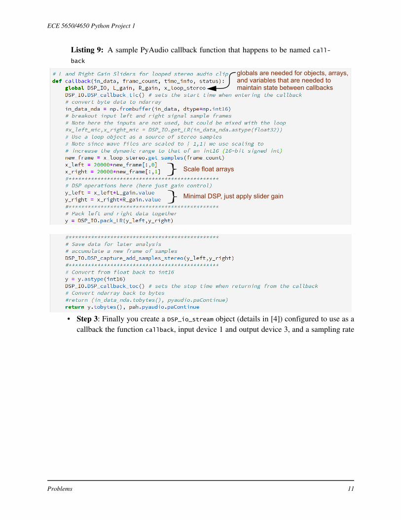
Listing 9: A sample PyAudio callback function that happens to be named call-back

• Step 3: Finally you create a DSP_io_stream object (details in [4]) configured to use as acallback the function callback, input device 1 and output device 3, and a sampling rate

Minimal DSP, just apply slider gain

Scale float arrays

globals are needed for objects, arrays, and variables that are needed tomaintain state between callbacks

Problems 11

ECE 5650/4650 Python Project 1

of 44.1 kHz. Figure 5 shows the code cell and a screen shot of the widgets as rendered in

the notebook. The first line of code brings in a stereo wave file and the second lineinstantiates an audio looping object. When instantiating the DSP_IO object it is best to setthe size of the capture buffer to 0s, this avoids memory issues when used in combinationwith setting the interactive stream to run indefinitely. Conversely, when setting Tcapture> 0, it is best to set Tsec to a similar value, but not less than Tcapture.

The Jupyter notebook Project1_pyaudio_helper_sample.ipynb, in the project ZIP package,contains the stereo audio loop example discussed in the steps 0–3 above. The framework forparts (a), (b), and (c) of Project Problem 5 can also be found in this notebook.

When you run the three cells and then click the Start Streaming button, hearing is believ-ing. What I mean is you have to listen through the playback device (speaks or headphones)to know things are really working. Actually, by analyzing the capture buffer you plot in thetime and frequency domain, or both via the spectrogram (specgram in matplotlib). TheProject1_pyaudio_helper_sample notebook discusses how to fill the capture bufferDSP_IO.data_capture_left, DSP_IO.data_capture_left for numChan = 2, or DSP_IO.data_-capture in the case of numChan = 1. Screen shots of the code cells and resulting graphics ofthe waveforms are given in Figure 6.

Usually 0 unless filling a capture buffer; avoids memorymanagement issues with RAM

Tsec = 0 for infinite capture, numChan = 2 for two channels

Usually 0 unless filling a capture buffer; avoids memorymanagement issues with RAM

Figure 5: A code cell example for Step 3 also include a screen shot of the result-ing widgets that are created when the cell is executed. Note when you first opena notebook the widgets are not displayed and you likely will see:

Error creating widget: could not find model

Error creating widget: could not find model

Problems 12

ECE 5650/4650 Python Project 1

A spectrogram example can be found in Project1_pyaudio_helper_sample as well a quicklook at stream callback statistics.

Now its time to write some code.

Using the LinearChirp Class in pyaudio_helper

a) In this first exercise you are going to interface a pre-made software component in apyaudio_helper callback to create a parameterizable linear frequency chirp on the leftchannel and a variable frequency sinusoid on the right channel. The component isincluded in Project1_pyaudio_helper_sample under Section 5a.

A linear chirp signal is created when you sweep the frequency of a sinusoidal waveform

Figure 6: Working with the capture DSP_io_stream.data_capture buffer whennumChan = 2 and displaying the left and right channel waveforms.

Problems 13

ECE 5650/4650 Python Project 1

linearly from a starting frequency, , to an ending frequency, , over a time inter-val . The process repeats at rate with a sawtooth shaped waveform, i.e.,

In continuous time the signal takes the form

(7)

which has instantaneous frequency

Hz (8)

A discrete-time implementation of is found in the class LinearChirp, Listing 10below.

Listing 10: Code listing of the LinearChirp class which is used in Problem 5a.

class LinearChirp(object): """ The class for creating a linear chirp signal that can be used in frame-based processing, such as PyAudio. Mark Wickert November 2018 """ def __init__(self, f_start, f_stop, period=1.0, frame_length = 1024, fs=48000): """ Instantiate a chirp object """ self.f_start = f_start self.f_stop = f_stop self.period = period self.fs = fs self.frame_length = frame_length # State variables self.theta = zeros(self.frame_length) self.theta_old = 0 self.f_ramp_old = 0 if self.period > 0: self.Df = self.f_stop - self.f_start self.f_step = self.Df/(self.period*self.fs) def generate(self): """ Generate an array of samples

fstart fstopTp Rp 1 Tp=

t

f inst

fmin

fmax

0 Tp 2Tp

. . .

Figure 7: The instantaneous frequency of a linear chirp sinusoid.

x t A 2fstartt 2t2 + + cos=

fi t 12------ d

dt----- 2fstartt 2t2 + + fstart 2t+= =

x t

Problems 14

ECE 5650/4650 Python Project 1

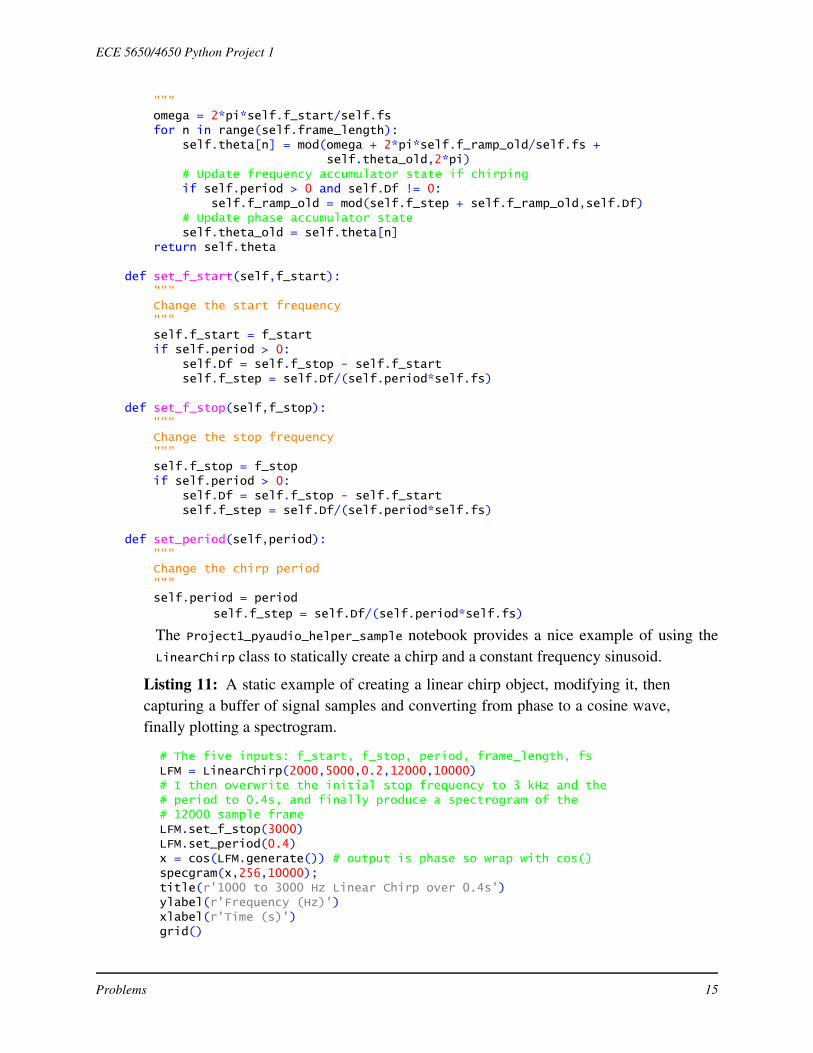
""" omega = 2*pi*self.f_start/self.fs for n in range(self.frame_length): self.theta[n] = mod(omega + 2*pi*self.f_ramp_old/self.fs + self.theta_old,2*pi) # Update frequency accumulator state if chirping if self.period > 0 and self.Df != 0: self.f_ramp_old = mod(self.f_step + self.f_ramp_old,self.Df) # Update phase accumulator state self.theta_old = self.theta[n] return self.theta def set_f_start(self,f_start): """ Change the start frequency """ self.f_start = f_start if self.period > 0: self.Df = self.f_stop - self.f_start self.f_step = self.Df/(self.period*self.fs) def set_f_stop(self,f_stop): """ Change the stop frequency """ self.f_stop = f_stop if self.period > 0: self.Df = self.f_stop - self.f_start self.f_step = self.Df/(self.period*self.fs) def set_period(self,period): """ Change the chirp period """ self.period = period

self.f_step = self.Df/(self.period*self.fs)

The Project1_pyaudio_helper_sample notebook provides a nice example of using theLinearChirp class to statically create a chirp and a constant frequency sinusoid.

Listing 11: A static example of creating a linear chirp object, modifying it, thencapturing a buffer of signal samples and converting from phase to a cosine wave,finally plotting a spectrogram.

# The five inputs: f_start, f_stop, period, frame_length, fsLFM = LinearChirp(2000,5000,0.2,12000,10000)# I then overwrite the initial stop frequency to 3 kHz and the # period to 0.4s, and finally produce a spectrogram of the # 12000 sample frameLFM.set_f_stop(3000)LFM.set_period(0.4)x = cos(LFM.generate()) # output is phase so wrap with cos()specgram(x,256,10000);title(r'1000 to 3000 Hz Linear Chirp over 0.4s')ylabel(r'Frequency (Hz)')xlabel(r'Time (s)')grid()

Problems 15

ECE 5650/4650 Python Project 1

Figure 8 shows the result spectrogram is an indeed a linear chirp running from 2 kHz to3 KHz with a period of 400 ms.

Moving on, the Problem 5a task is to implement a two channel real-time audio signalgenerator, with the left channel producing a linear chirp and the right channel producinga sinusoid, both tunable. Figure 9 shows the Step 3 code cell and widgets.

Figure 8: Spectrogram of a statically created linear chirp created using a 12000sample frame.

• L/R gain min = 0, max = 2,step = 0.01

• Chirp rate ( ) min 0.5Hz, max = 100 Hz, step = 0.1Hz

• The three frequency slidersmin = 10 Hz, max = 12000Hz, step = 1.0 Hz

1 Tp

Figure 9: The Step 3 code cell and a screen shot of the widgets required forProblem 5a.

Problems 16

ECE 5650/4650 Python Project 1

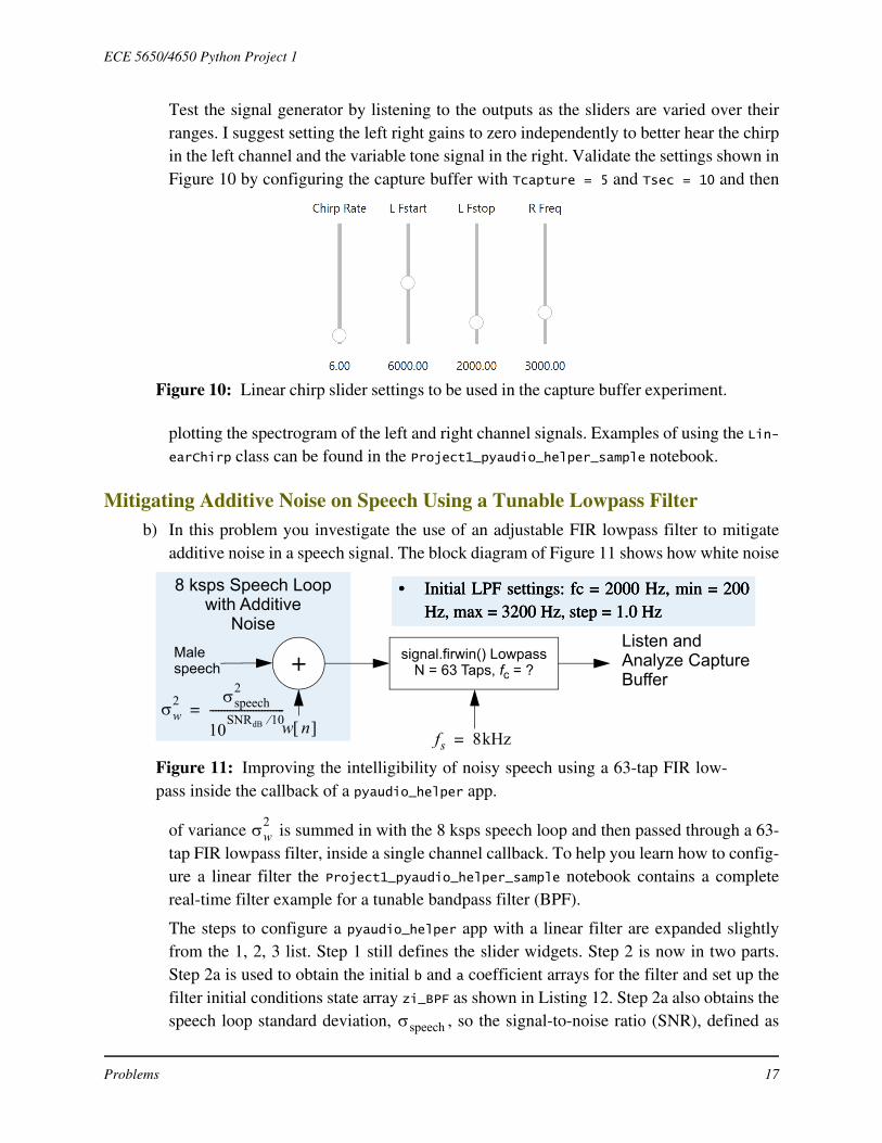
Test the signal generator by listening to the outputs as the sliders are varied over theirranges. I suggest setting the left right gains to zero independently to better hear the chirpin the left channel and the variable tone signal in the right. Validate the settings shown inFigure 10 by configuring the capture buffer with Tcapture = 5 and Tsec = 10 and then

plotting the spectrogram of the left and right channel signals. Examples of using the Lin-earChirp class can be found in the Project1_pyaudio_helper_sample notebook.

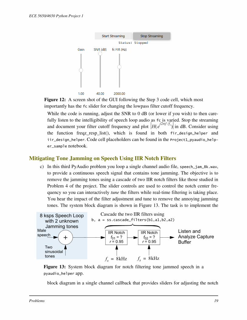
Mitigating Additive Noise on Speech Using a Tunable Lowpass Filterb) In this problem you investigate the use of an adjustable FIR lowpass filter to mitigate

additive noise in a speech signal. The block diagram of Figure 11 shows how white noise

of variance is summed in with the 8 ksps speech loop and then passed through a 63-tap FIR lowpass filter, inside a single channel callback. To help you learn how to config-ure a linear filter the Project1_pyaudio_helper_sample notebook contains a completereal-time filter example for a tunable bandpass filter (BPF).

The steps to configure a pyaudio_helper app with a linear filter are expanded slightlyfrom the 1, 2, 3 list. Step 1 still defines the slider widgets. Step 2 is now in two parts.Step 2a is used to obtain the initial b and a coefficient arrays for the filter and set up thefilter initial conditions state array zi_BPF as shown in Listing 12. Step 2a also obtains thespeech loop standard deviation, , so the signal-to-noise ratio (SNR), defined as

Figure 10: Linear chirp slider settings to be used in the capture buffer experiment.

+ signal.firwin() LowpassN = 63 Taps, fc = ?

8 ksps Speech Loopwith Additive

Noise

Malespeech

Listen andAnalyze CaptureBuffer

Figure 11: Improving the intelligibility of noisy speech using a 63-tap FIR low-pass inside the callback of a pyaudio_helper app.

w n w2 speech

2

10SNRdB 10

--------------------------=

fs 8kHz=

• Initial LPF settings: fc = 2000 Hz, min = 200Hz, max = 3200 Hz, step = 1.0 Hz

• Initial LPF settings: fc = 2000 Hz, min = 200Hz, max = 3200 Hz, step = 1.0 Hz

• Initial LPF settings: fc = 2000 Hz, min = 200Hz, max = 3200 Hz, step = 1.0 Hz

w2

speech

Problems 17

ECE 5650/4650 Python Project 1

, is properly calibrated on-the-fly in the callback. The details can befound in Listing 13 and in Project1_pyaudio_helper_sample.

Listing 12: Step 2a code cell listing for the BPF example, showing in particularthe initial filter design and setting up the filter initial condition array which is usedto maintain filter state continuity when entering and departing the callback.

fs, x_rec = ss.from_wav('speech_8k.wav')std_x = std(x_rec) # For setting SNR# Design a bandpass filterb_BPF, a_BPF = H_BP(8000,1000)zi_BPF = signal.lfiltic(b_BPF, a_BPF,[0])ss.zplane(b_BPF, a_BPF) # take a look at the filter pole-zero plot

Set 2b is devoted to the callback function, which now is expanded to include not onlyreal-time filtering, but on-the-fly redesign of the filter should the GUI sliders be tweakedwhile code is running in real-time. Note five new global variables are needed to supportthe BPF: (2) GUI sliders and (3) filter related; two filter coefficient arrays and the initialconditions array. The details are in the code highlights of Listing 13.

Listing 13: Code cell highlights for Step 2b, the callback, for the tunable band-pass filter.

global DSP_IO, x_loop, Gain, std_x, SNR global BOF_f0, BPF_Df # remove/add globals for slider widgets

global b_BPF, a_BPF, zi_BPF #remove/add globals for filter related variables ...# Note wav is scaled to [-1,1] so need to rescale to int16

x = 32767*x_loop.get_samples(frame_count) x += 32767*std_x/10**(SNR.value/20) * randn(frame_count) # Perform real-time DSP, e.g. a linear filter b_BPF, a_BPF = H_BP(BPF_f0.value,BPF_Df.value)

y, zi_BPF = signal.lfilter(b_BPF,a_BPF,x,zi=zi_BPF)

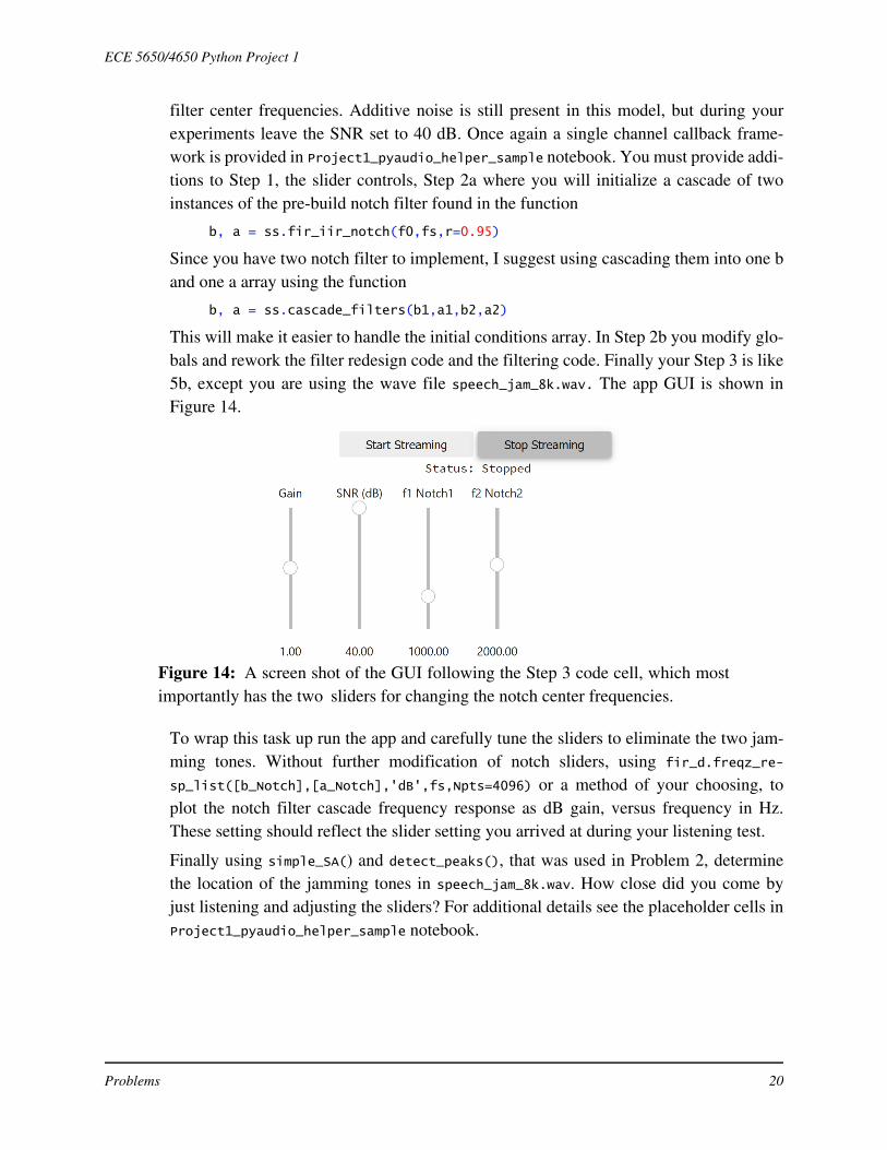
Moving on to the actual lowpass design of Problem 5b, you begin by implementing the63-tap lowpass and allow for on-the-fly changes in the cutoff frequency fc via a GUIslider. To start with, the filter design is implemented using the scipy.signal function b =signal.firwin(numtaps, cutoff, fs=8000), with all frequencies in Hz. To get thingsstarted an initial filter design, based the GUI slider initial values, is designed in Step 2balong with an initial state array zi_LPF. In Step 2b you remove/add globals for the slidersand add/remove filter related variables, then write filter redesign code, and filter usinginitial conditions. Finally in Step 3 you implement a code cell identical to the BPFexample above. Figure 12 shows the GUI that follows the Step 3 code cell. The attributesof the fc slider can be Found in Figure 11.

SNR speech2 w

2=

Problems 18

ECE 5650/4650 Python Project 1

While the code is running, adjust the SNR to 0 dB (or lower if you wish) to then care-fully listen to the intelligibility of speech loop audio as fc is varied. Stop the streamingand document your filter cutoff frequency and plot in dB. Consider usingthe function freqz_resp_list(), which is found in both fir_design_helper andiir_design_helper. Code cell placeholders can be found in the Project1_pyaudio_help-er_sample notebook.

Mitigating Tone Jamming on Speech Using IIR Notch Filtersc) In this third PyAudio problem you loop a single channel audio file, speech_jam_8k.wav,

to provide a continuous speech signal that contains tone jamming. The objective is toremove the jamming tones using a cascade of two IIR notch filters like those studied inProblem 4 of the project. The slider controls are used to control the notch center fre-quency so you can interactively tune the filters while real-time filtering is taking place.You hear the impact of the filter adjustment and tune to remove the annoying jammingtones. The system block diagram is shown in Figure 13. The task is to implement the

block diagram in a single channel callback that provides sliders for adjusting the notch

Figure 12: A screen shot of the GUI following the Step 3 code cell, which mostimportantly has the fc slider for changing the lowpass filter cutoff frequency.

H ej2f fs

+IIR Notch

f01 = ?r = 0.95

IIR Notchf02 = ?r = 0.95

8 ksps Speech Loopwith 2 unknownJamming tones

Malespeech

Two sinusoidal tones

Listen andAnalyze CaptureBuffer

Figure 13: System block diagram for notch filtering tone jammed speech in apyaudio_helper app.

Cascade the two IIR filters using b, a = ss.cascade_filters(b1,a1,b2,a2)

fs 8kHz= fs 8kHz=

Problems 19

ECE 5650/4650 Python Project 1

filter center frequencies. Additive noise is still present in this model, but during yourexperiments leave the SNR set to 40 dB. Once again a single channel callback frame-work is provided in Project1_pyaudio_helper_sample notebook. You must provide addi-tions to Step 1, the slider controls, Step 2a where you will initialize a cascade of twoinstances of the pre-build notch filter found in the function

b, a = ss.fir_iir_notch(f0,fs,r=0.95)

Since you have two notch filter to implement, I suggest using cascading them into one band one a array using the function

b, a = ss.cascade_filters(b1,a1,b2,a2)

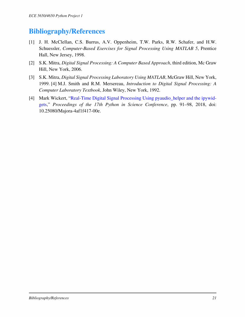
This will make it easier to handle the initial conditions array. In Step 2b you modify glo-bals and rework the filter redesign code and the filtering code. Finally your Step 3 is like5b, except you are using the wave file speech_jam_8k.wav. The app GUI is shown inFigure 14.

To wrap this task up run the app and carefully tune the sliders to eliminate the two jam-ming tones. Without further modification of notch sliders, using fir_d.freqz_re-sp_list([b_Notch],[a_Notch],'dB',fs,Npts=4096) or a method of your choosing, toplot the notch filter cascade frequency response as dB gain, versus frequency in Hz.These setting should reflect the slider setting you arrived at during your listening test.

Finally using simple_SA() and detect_peaks(), that was used in Problem 2, determinethe location of the jamming tones in speech_jam_8k.wav. How close did you come byjust listening and adjusting the sliders? For additional details see the placeholder cells inProject1_pyaudio_helper_sample notebook.

Figure 14: A screen shot of the GUI following the Step 3 code cell, which mostimportantly has the two sliders for changing the notch center frequencies.

Problems 20

ECE 5650/4650 Python Project 1

Bibliography/References [1] J. H. McClellan, C.S. Burrus, A.V. Oppenheim, T.W. Parks, R.W. Schafer, and H.W.

Schuessler, Computer-Based Exercises for Signal Processing Using MATLAB 5, PrenticeHall, New Jersey, 1998.

[2] S.K. Mitra, Digital Signal Processing: A Computer Based Approach, third edition, Mc GrawHill, New York, 2006.

[3] S.K. Mitra, Digital Signal Processing Laboratory Using MATLAB, McGraw Hill, New York,1999. [4] M.J. Smith and R.M. Mersereau, Introduction to Digital Signal Processing: AComputer Laboratory Textbook, John Wiley, New York, 1992.

[4] Mark Wickert, “Real-Time Digital Signal Processing Using pyaudio_helper and the ipywid-gets,” Proceedings of the 17th Python in Science Conference, pp. 91–98, 2018, doi:10.25080/Majora-4af1f417-00e.

Bibliography/References 21