ECE 2221 SIGNALS AND SYSTEMS - International …staff.iium.edu.my/sigit/ece2221/pdf/02 Continuous...
72
ECE 2221 SIGNALS AND SYSTEMS ECE 2221 Signals and Systems, Sem 3 2010/2011, Dr. Sigit Jarot 1
Transcript of ECE 2221 SIGNALS AND SYSTEMS - International …staff.iium.edu.my/sigit/ece2221/pdf/02 Continuous...
E C E 2 2 2 1 S I G N A L S A N D S Y S T E M S
ECE 2221 Signals and Systems, Sem 3 2010/2011, Dr. Sigit Jarot
1

Course Objectives
Dr. Sigit PW JarotECE 2221 Signals and Systems 2
To provide an analysis skill of the continuous‐time signals and systems as reflected to their roles in engineering
practice.
To expose students to both the time‐domain and frequency‐domain methods of analyzing signals and
systems.
To illustrate the potential applications of this course as a Pre‐requisite course to communication engineering and principles, digital signal processing and control system.

OBE (Outcome Based Education)Learning Outcomes
Dr. Sigit PW JarotECE 2221 Signals and Systems 3
Classify, characterize and conduct basic of signals and systems.
Analyze continuous‐time signals and systems in time domain using convolution.
Analyze continuous‐time signals and systems in frequency domain using Laplace transform.
Analyze continuous‐time signals and systems in frequency domain using Fourier series and Fourier transform.
Acquire introductory‐level knowledge of discrete‐time signals and systems, and sampling theory.
Work in group to perform basic simulation of signals and systems analysis.
After completion of this course the students will be able to:

Course Synopsis
Dr. Sigit PW JarotECE 2221 Signals and Systems 4
Introduction to Signals
Introduction to Systems
Time‐Domain Analysis of Continuous‐Time Systems
Frequency‐Domain System Analysis: the Laplace Transform
MID‐TERM Examination
Signals Analysis using the Fourier Series
Signals Analysis using the Fourier Transform
Introduction to Discrete Time Signals and Systems Analysis
FINAL Examination
Outline
ECE 2221 Signals and Systems, Sem 3 2010/2011, Dr. Sigit Jarot
5
Concept of system and system classification Linear time‐invariant continuous‐time systems Linearity and time‐invariance Causality and stability
System Representation Systems represented by differential equations Convolution integral
System interconnection

System Concept
ECE 2221 Signals and Systems, Sem 3 2010/2011, Dr. Sigit Jarot
6
System is a mathematical transformation of an input signal (or signals) into an output signal (or signals)
SIGNAL A set of data or information. A function or sequence of values that represents information. A function of one or more variables (e.g. time, frequency, space,..) that conveys information on the nature of a physical phenomenon.
SYSTEM A system is an entity that processes a set of signals (inputs) to yield another sets of signals (outputs)
SystemInputSignal
OutputSignal

System Classification
ECE 2221 Signals and Systems, Sem 3 2010/2011, Dr. Sigit Jarot
7
Static or Dynamic Systems A dynamic system has the capability of storing energy, or remembering its
state, while a static system does not. A battery connected to resistors is a static system, while the same battery
connected to resistors, capacitors, and inductors constitutes a dynamic system.
The main difference is the capability of capacitors and inductors to store energy, to remember the state of the device, that resistors do not have.
Continuous‐Time or Discrete‐Time System Whenever the input(s) and output(s) are both continuous time, discrete
time, or digital, the corresponding systems are continuous time, discrete time, or digital, respectively.
It is also possible to have hybrid systems when the input(s) and output(s) are not of the same type.

LTI Continuous Time Systems
ECE 2221 Signals and Systems, Sem 3 2010/2011, Dr. Sigit Jarot
8
A continuous‐time system is a system in which the signals at its input and output are continuous‐time signals.
Mathematically we represent it as a transformation S that converts an input signal x(t) into an output signal y(t)=S[x(t)]

Characteristics of System Models
ECE 2221 Signals and Systems, Sem 3 2010/2011, Dr. Sigit Jarot
9
Linearity The linearity between the input and the output, as well as the constancy of
the system parameters, simplify the mathematical model.
Time invariance Causality Causality, or nonanticipatory behavior of the system, relates to the cause–
effect relationship between the input and the output. It is essential when the system is working under real‐time situations—that is, when there is limited time for the system to process signals coming into the system.
Stability Stability is needed in practical systems. A stable system behaves well under
reasonable inputs. Unstable systems are useless.

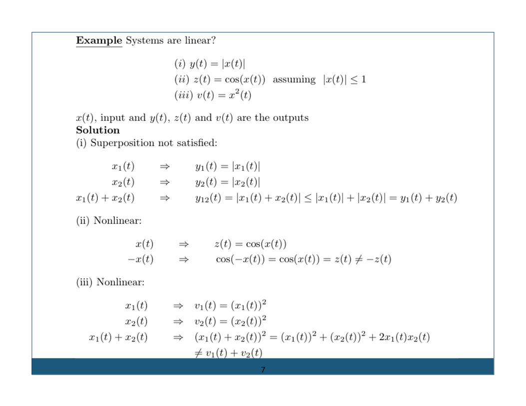
Linearity
ECE 2221 Signals and Systems, Sem 3 2010/2011, Dr. Sigit Jarot
10
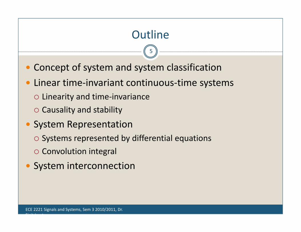
A system is said to be linear in terms of the system input (excitation) x(t) and the system output (response) y(t) if it satisfies the following two properties of superposition and homogeneity:1. Superposition:
1( ) ( )x t x t 1( ) ( )y t y t
2( ) ( )x t x t 2( ) ( )y t y t1 2( ) ( ) ( )x t x t x t
1 2( ) ( ) ( )y t y t y t 2. Homogeneity:
( )x t ( )y t ( )ax t ( )ay ta = constant
factor
ECE 2221 Signals and Systems, Sem 3 2010/2011, Dr. Sigit Jarot
11
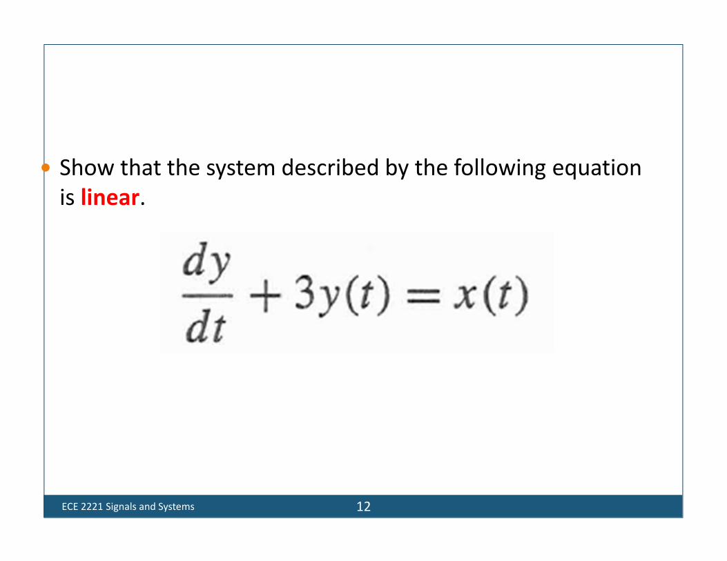
ECE 2221 Signals and Systems 12
Show that the system described by the following equation is linear.

ECE 2221 Signals and Systems 13
Show that the system described by the equation is linear.
Let x1(t) → y1(t) and x2(t) → y2(t), then and
Multiple 1st equation by k1, and 2nd equation by k2, and adding them yields:
This equation is the system equation with and

7
7

Time Invariance16
A system is said to be time invariance if a time delay or time advance of the input signal leads to an identical time shift in the output signal.
A time‐invariant system do not change with time.
The notion of time invariance. (a) Time‐shift operator St0 preceding operator H. (b) Time‐shift operator St0 following operator H. These two situations are equivalent,
provided that H is time invariant.

ECE 2221 Signals and Systems, Sem 3 2010/2011, Dr. Sigit Jarot
17
ECE 2221 Signals and Systems, Sem 3 2010/2011, Dr. Sigit Jarot
18

19
Time InvarianceExample : Inductor
x1(t) = v(t)
y1(t) = i(t)
The inductor shown in figure is described by the input‐output relation:
1 11( ) ( )
ty t x d
L
where L is the inductance. Show that the inductor so described is time invariant.<Sol.>1. Let x1(t) x1(t t0) Response y2(t) of the inductor to x1(t t0) is
0
1 0 11( ) ( )
t ty t t x d
L
2 1 01( ) ( )
ty t x t d
L
2. Let y1(t t0) = the original output of the inductor, shifted by t0 seconds:
3. Changing variables: 0' t
(A)
(B)
(A)0
2 11( ) ( ') '
t ty t x d
L
Inductor is time invariant.

20
Time InvarianceExample : Inductor
x1(t) = v(t)
y1(t) = i(t)
The inductor shown in figure is described by the input‐output relation:
1 11( ) ( )
ty t x d
L
where L is the inductance. Show that the inductor so described is time invariant.<Sol.>1. Let x1(t) x1(t t0) Response y2(t) of the inductor to x1(t t0) is
0
1 0 11( ) ( )
t ty t t x d
L
2 1 01( ) ( )
ty t x t d
L
2. Let y1(t t0) = the original output of the inductor, shifted by t0 seconds:
3. Changing variables: 0' t
(A)
(B)
(A)0
2 11( ) ( ') '
t ty t x d
L
Inductor is time invariant.

Signals_and_Systems_Simon Haykin & Barry Van Veen 21
Time InvarianceExample Thermistor
Let R(t) denote the resistance of the thermistor, expressed as a function of time. We may express the input‐output relation of the device as
x1(t) = v(t)
y1(t) = i(t)
1 1( ) ( ) / ( )y t x t R tShow that the thermistor so described is time variant.<Sol.>1. Let response y2(t) of the thermistor to x1(t t0) is
1 02
( )( )( )
x t ty tR t
2. Let y1(t t0) = the original output of the thermistor due to x1(t), shifted by t0seconds:
1 01 0
0
( )( )( )
x t ty t tR t t
3. Since R(t) R(t t0) 1 0 2 0( ) ( ) for 0y t t y t t Time variant!
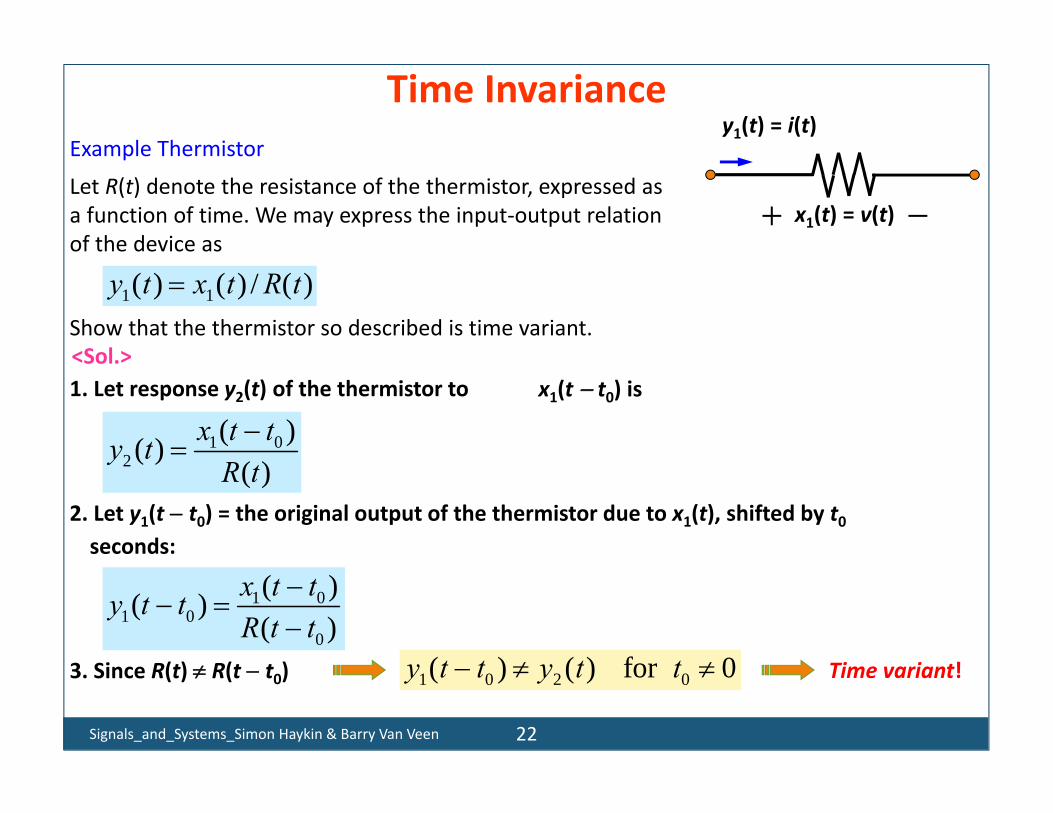
Signals_and_Systems_Simon Haykin & Barry Van Veen 22
Time InvarianceExample Thermistor
Let R(t) denote the resistance of the thermistor, expressed as a function of time. We may express the input‐output relation of the device as
x1(t) = v(t)
y1(t) = i(t)
1 1( ) ( ) / ( )y t x t R tShow that the thermistor so described is time variant.<Sol.>1. Let response y2(t) of the thermistor to x1(t t0) is
1 02
( )( )( )
x t ty tR t
2. Let y1(t t0) = the original output of the thermistor due to x1(t), shifted by t0seconds:
1 01 0
0
( )( )( )
x t ty t tR t t
3. Since R(t) R(t t0) 1 0 2 0( ) ( ) for 0y t t y t t Time variant!

ECE 2221 Signals and Systems, Sem 3 2010/2011, Dr. Sigit Jarot
23

ECE 2221 Signals and Systems, Sem 3 2010/2011, Dr. Sigit Jarot
24

ECE 2221 Signals and Systems, Sem 3 2010/2011, Dr. Sigit Jarot
25

Causality
ECE 2221 Signals and Systems, Sem 3 2010/2011, Dr. Sigit Jarot
26
Causality is independent of the linearity and the time‐invariance properties of a system.
Representation of Systems by Differential Equations
ECE 2221 Signals and Systems, Sem 3 2010/2011, Dr. Sigit Jarot
27

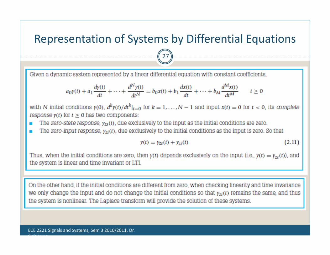
Response of a Linear System
A system’s output for t ≥ 0 is the result of 2 independent causes:1. The initial condition at t = 0 zero‐input response2. The input x(t) for t ≥ 0 zero‐state response
Decomposition property:
Total response = zero‐input response + zero‐state response
x(t) y(t) +y0(t) x(t) ys(t)=
t
C tdxC
tRxvty0
0)(1)()0()(
zero‐input response zero‐state response
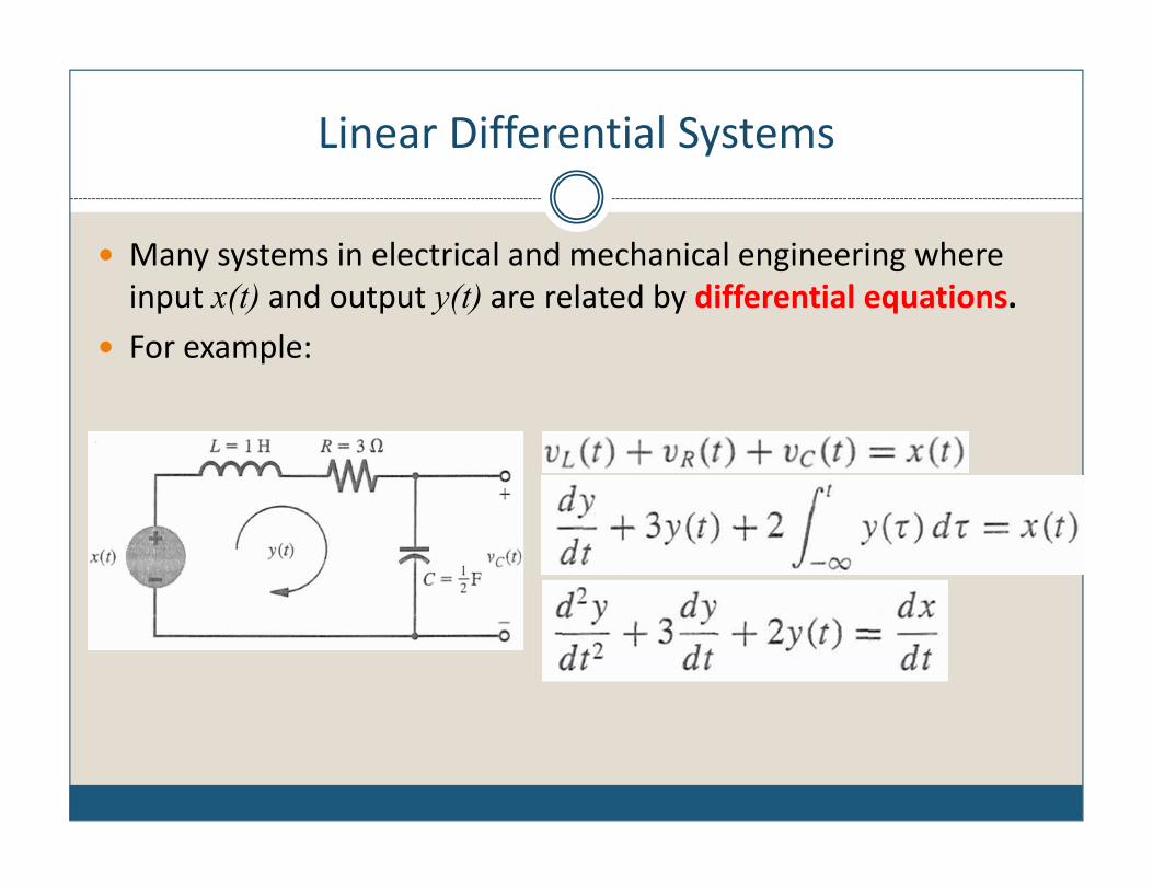
Linear Differential Systems
Many systems in electrical and mechanical engineering where input x(t) and output y(t) are related by differential equations.
For example:

Linear Differential Systems
In general, relationship between x(t) and y(t) in a linear time‐invariant (LTI) differential system is given by (where all coefficients ai and bi are constants):
Use compact notation D for operator d/dt, i.e.
We get
or
)(...)(... 11
1
111
1
1 txbdtdxb
dtxdb
dtxdbtya
dtdya
dtyda
dtyd
NNM
M
MNM
M
MNNNN
N
N
N
.)()( 22
2
etctyDdt
ydandtDydtdy
)()...()()...( 11
111
1 txbDbDbDbtyaDaDaD NNM
MNM
MNNNNN
)()()()( txDPtyDQ
NNM
MNM
MN
NNNN
bDbDbDbDP
aDaDaDDQ
11
1
11
1
...)(
...)(

Zero‐input response basics
Remember that for a Linear System
In this lecture, we will focus on a linear system’s zero‐input response, y0(t), which is the solution of the system equation when input x(t)=0.
Recall
For zero‐input response
Total response = zero‐input response + zero‐state response
)()...()()...( 11
111
1 txbDbDbDbtyaDaDaD NNM
MNM
MNNNNN
)()()()( txDPtyDQ
0)()( 0 tyDQ
0)()...( 011
1 tyaDaDaD NN
NN

General solutions to the zero‐input response equation (1)
From math course on differential equations, we may solve the equation:
By letting where c and λ are constant. Then, by substituting into the above equation
0)()...( 011
1 tyaDaDaD NN
NN
tcety )(0
tNN
NN
t
t
ecdt
ydtyD
ecdt
ydtyD
ecdt
dytDy
00
22
02
02
00
)(
)(
)(

General solutions to the zero‐input response equation (2)
We get
This is identical to the polynomial Q(D) with λ replacing D, i.e.
We can now express Q(λ) in factorized form:
Therefore λ has solutions: λ1, λ2,… λN assuming that all λi are distinct.

General solutions to the zero‐input response equation (3)
Therefore,
has N possible solutions:
where are arbitrarily constants.
It can be shown that the general solution is the sum of all these terms:
In order to determine the N arbitrary constant, we need to have N constraints(i.e. initial or boundary or auxiliary conditions).
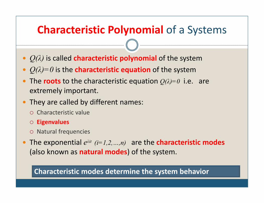
Characteristic Polynomial of a Systems
Q(λ) is called characteristic polynomial of the system Q(λ)=0 is the characteristic equation of the system The roots to the characteristic equation Q(λ)=0 i.e. are extremely important.
They are called by different names: Characteristic value Eigenvalues Natural frequencies
The exponential eλit (i=1,2,…,n) are the characteristic modes(also known as natural modes) of the system.
Characteristic modes determine the system behavior

ECE 2221 Signals and Systems
36

ECE 2221 Signals and Systems
37

ECE 2221 Signals and Systems
38

Repeated Characteristic Roots
If there are repeated roots, the form of the solution is modified.
The solution of the equation:
is given by
In general, the characteristic modes for the differential equation:
are
The solution for yo(t) is

ECE 2221 Signals and Systems
40

ECE 2221 Signals and Systems
41

Complex Characteristic Roots
Solution of the characteristic equation may result in complex roots. For real (i.e. physically realizable) systems, all complex roots must occur in
conjugate pairs In other words, the coefficients of the characteristic polynomial Q(λ) are real.
In other words, if α+jβ is a root, the there must exist the root α-jβ . The zero‐input response corresponding to this pair of conjugate roots is:
For a real system, the response yo(t) must also be real. This is possible only if c1 and c2 are conjugates too.
Let
This gives
ECE 2221 Signals and Systems
43

ECE 2221 Signals and Systems
44

ECE 2221 Signals and Systems
45

The meaning of 0‐ and 0+
There are subtle differences between time t = 0 exactly, time just before t=0, i.e. t = 0‐ and time just AFTER t=0, i.e. t = 0+.
At t = 0‐ the total response y(t) consists SOLELY of the zero‐input component y0(t).
However, applying an input x(t) at t=0, while not affecting y0(t), in general WILL affect y(t) (because input is now no longer zero).
ECE 2221 Signals and Systems
46

Insight into Zero‐input Behavior
Assume a system is initially at rest. Now disturb it momentarily, then remove the disturbance (now it is zero‐input), the system will not come back to rest instantaneously.
In generally, it will go back to rest over a period of time, and only through some special type of motion that is characteristic of the system.
Such response must be sustained without any external source (because the disturbance has been removed).
In fact the system uses a linear combination of the characteristic modes to come back to the rest position while satisfying some boundary (or initial) conditions.
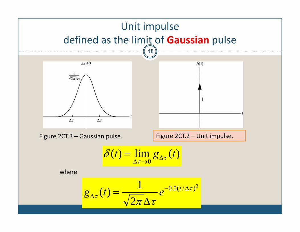
Unit impulse defined as the limit of Gaussian pulse
48
Figure 2CT.2 – Unit impulse.
)(lim)(0
tgt
Figure 2CT.3 – Gaussian pulse.
2)/(5.0
21)(
tetg
where

Sampling Property of Unit Impulse49
If you multiply an arbitrary waveform x(t) by an impulse occurring at time , you obtain an impulse have area x() occurring at time .
We can view the impulse as “sampling” x(t) at t =.
Figure 2CT.8 – Sampling property of the unit impulse
)()()()( txttx

Impulse Response50
The response of a LTIC system to a unit impulse is called the system’s impulse response and is denoted as h(t) .
)(t )(thUnit Impulse Impulse Response

Impulse Response of Integrator51
h(t) for t < 0 h(t) for t = 0 h(t) for t > 0
Figure 1.9 – Integrator.
Figure 2CT.9 – Region of integration for eq. (8) (shaded).
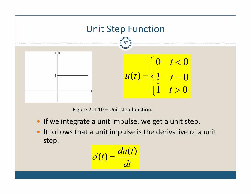
Unit Step Function52
If we integrate a unit impulse, we get a unit step. It follows that a unit impulse is the derivative of a unit step.
Figure 2CT.10 – Unit step function.
dttdut )()(
01000
)(21
ttt
tu

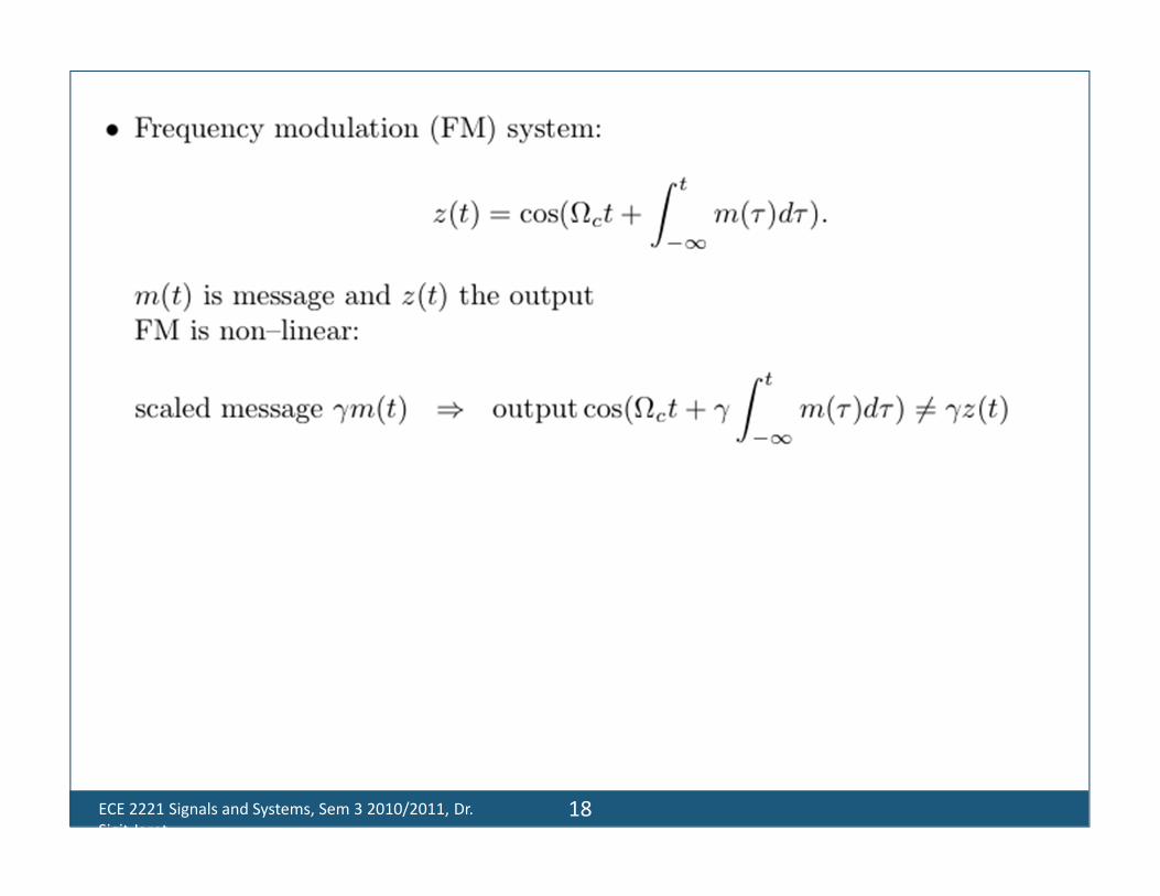
Nonlinear systems can be approximated by linear system
Almost all systems become nonlinear when large enough signals are applied Nonlinear systems can be approximated by linear systems for small‐signal analysis – greatly
simply the problem Once superposition applies, analyse system by decomposition into zero‐input and zerostate
components Equally important, we can represent x(t) as a sum of simpler functions (pulse or step)
ECE 2221 Signals and Systems
53
Outline
(Review of Previous Lecture) Zero‐Input Response
Unit Impulse Response Convolution Integral Total Response Summary

Response of a Linear System
A system’s output for t ≥ 0 is the result of 2 independent causes:1. The initial condition at t = 0 zero‐input response2. The input x(t) for t ≥ 0 zero‐state response
Decomposition property:
Total response = zero‐input response + zero‐state response
x(t) y(t) +y0(t) x(t) ys(t)=
t
C tdxC
tRxvty0
0)(1)()0()(
zero‐input response zero‐state response

The importance of Impulse Response h(t)
Zero‐state response assumes that the system is in “rest” state, i.e. all internal system variables are zero.
Deriving and understanding zero‐state response depends on knowing the impulse response h(t) to a system.
Any input x(t) can be broken into many narrow rectangular pulses. Each pulse produces a system response.
Since the system is linear and time invariant, the system response to x(t) is the sum of its responses to all the impulse components.
h(t) is the system response to the rectangular pulse at t=0 as the pulse width approaches zero.

Zero‐state Response (1)
We now consider how to determine the system response y(t) to an input x(t) when system is in zero state.
Define a pulse p(t) of unit height and width Δτ at t=0 .
Input x(t) can be represented as sum of narrow rectangular pulses.
The pulse at t=nΔτ has a height x(t)=x(nΔτ) . This can be expressed as x(nΔτ)p (t-nΔτ). Therefore x(t) is the sum of all [x(nΔτ)/ Δτ] . such
pulses, i.e,
)()(lim
)()(lim)(
0
0
ntpnx
ntpnxtx

Zero‐state Response (2)
The term [x(nΔτ)/ Δτ]p(t-nΔτ) represents a pulse p(t-nΔτ) with height x(nΔτ).
As Δτ 0, height of strip ∞, but area remain x(nΔτ) and
)()()()(
ntnxntpnx
)()(lim)(
0ntnxtx

Zero‐state Response (3)
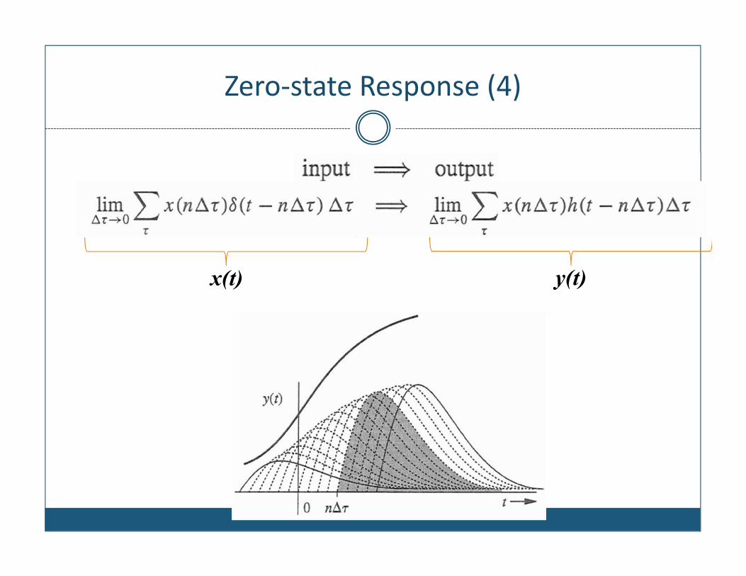
Zero‐state Response (4)
x(t) y(t)
Zero‐state Response (5)
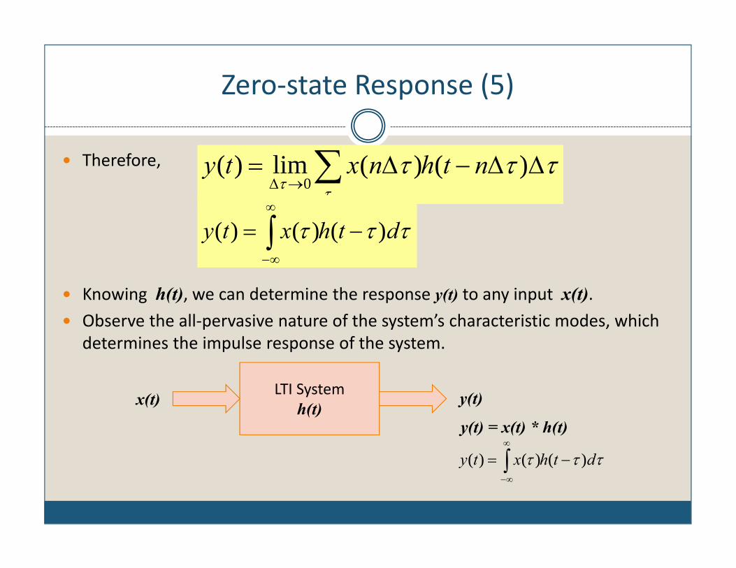
Therefore,
Knowing h(t), we can determine the response y(t) to any input x(t). Observe the all‐pervasive nature of the system’s characteristic modes, which
determines the impulse response of the system.
LTI Systemh(t)x(t) y(t)
y(t) = x(t) * h(t)
)()(lim)(
0nthnxty
dthxty )()()(
dthxty )()()(

How to determine the unit impulse response h(t) (1)
Given that a system is specified by the following differential equation, determine its unit impulse response h(t).
Remember the general system equation:
It can be shown that the impulse response h(t) is given by:
where u(t) is the unit step function, and yn(t) is a linear combination of the characteristic modes of the system.
)()()()( txDPtyDQ
)()]()([)( tutyDPth n
tN
ttn
Necececty ......)( 2121
dtdxty
dtdy
dtyd
)(232
2
How to determine the unit impulse response h(t)? (2)
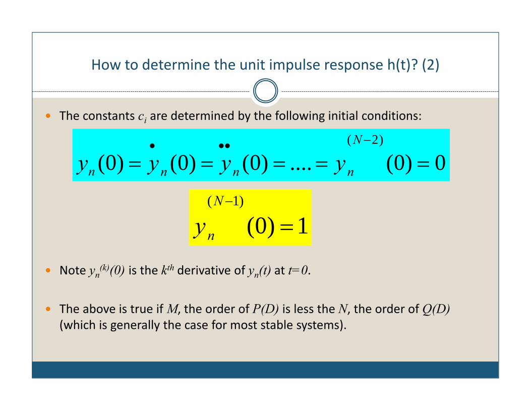
The constants ci are determined by the following initial conditions:
Note yn(k)(0) is the kth derivative of yn(t) at t=0.
The above is true if M, the order of P(D) is less the N, the order of Q(D)(which is generally the case for most stable systems).
0)0(....)0()0()0()2(
N
nnnn yyyy
1)0()1(
N
ny
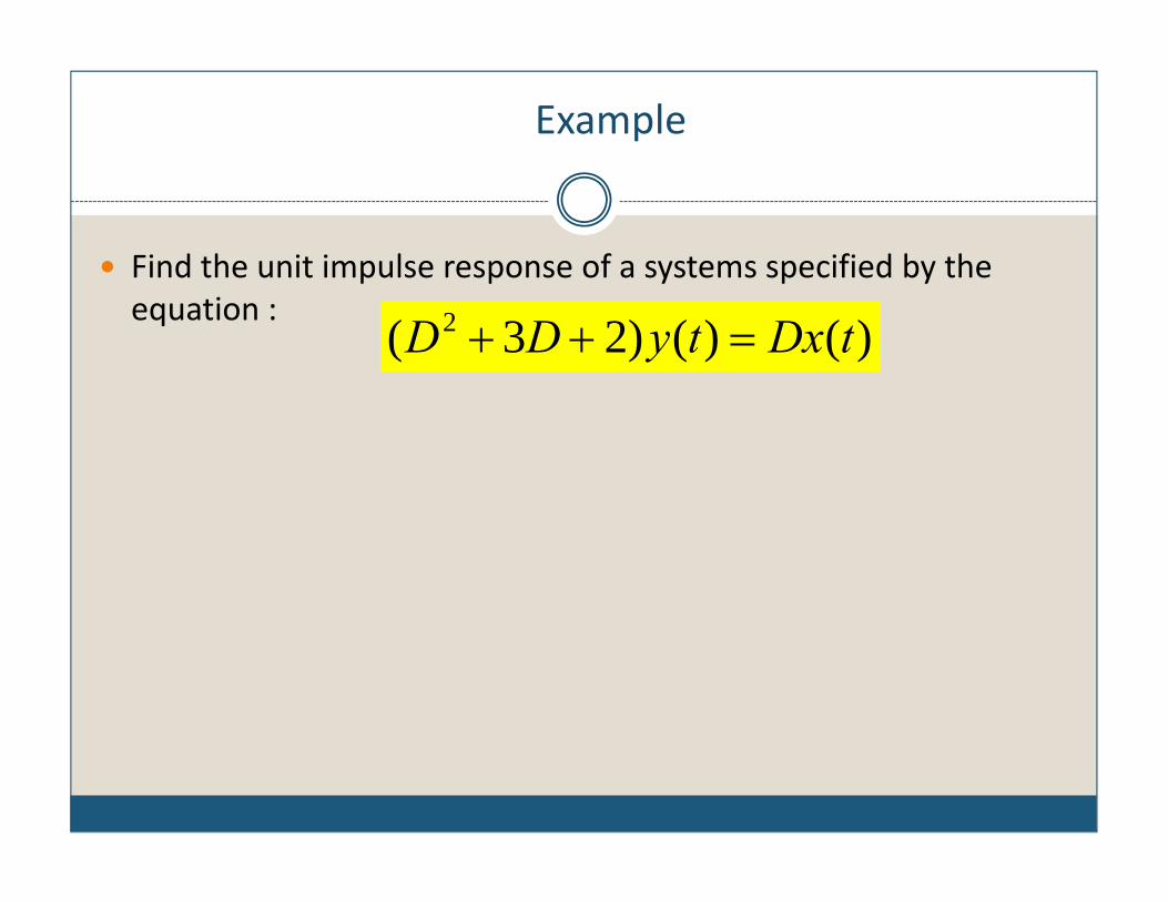
Example
Find the unit impulse response of a systems specified by the equation :
)()()23( 2 tDxtyDD
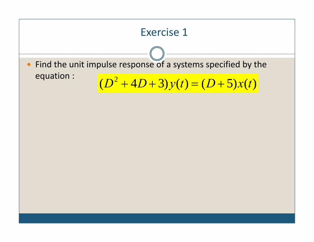
Exercise 1
Find the unit impulse response of a systems specified by the equation :
)()5()()34( 2 txDtyDD
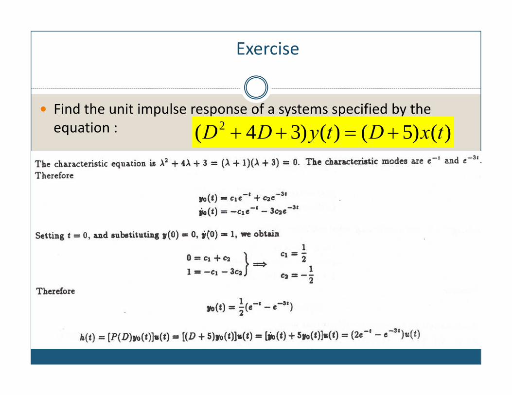
Exercise
Find the unit impulse response of a systems specified by the equation : )()5()()34( 2 txDtyDD

Exercise 2
Find the unit impulse response of a systems specified by the equation : )()117()()65( 22 txDDtyDD

Exercise Find the unit impulse response of a systems specified by the equation :
)()117()()65( 22 txDDtyDD

The Convolution Integral
The derived integral equation occurs frequently in physical sciences, engineering, and mathematics.
It is given the name: the convolution integral. The convolution integral of two function x1(t) and x2(t) is denoted symbolically as x1(t)* x2(t)
And is defined as
Note that the convolution operator is linear, i.e. it obeys the principle of superposition.
dtxxtxtx )()()()( 2121

Properties of Convolution (1)
Commutative Property (order of operands does not matter):
Associative Property (order of operator does not matter):
Distributive Property:

Properties of Convolution (2)
Shift Property: if
then
also
Impulse Property Convolution of a function x(t) with a unit impulse results in the function x(t).

Properties of Convolution (3)
Width Property: Duration of x1(t)=T1 , and duration of x2(t)=T2 , then duration of x1(t)*x2(t)=T1 + T2
Causality Property:


![Ece-IV-signals & Systems [10ec44]-Notes (1)](https://static.fdocuments.in/doc/165x107/577ccda41a28ab9e788c8c75/ece-iv-signals-systems-10ec44-notes-1.jpg)


![Ece IV Signals & Systems [10ec44] Solution](https://static.fdocuments.in/doc/165x107/55cf980d550346d033954979/ece-iv-signals-systems-10ec44-solution.jpg)

![Ece IV Signals & Systems [10ec44] Notes](https://static.fdocuments.in/doc/165x107/577cde381a28ab9e78aea92f/ece-iv-signals-systems-10ec44-notes.jpg)