DEPT/ YEAR/ SEM: ECE/ II/ IV

FATIMA MICHAEL COLLEGE OF ENGINEERIMG & TECHNOLOGY

EC2253

ELECTROMAGNETIC FIELDS

PREPARED BY: Mrs.K.Suganya/ Asst.Prof/ECE

EC2253 – ELECTROMAGNETIC FIELDS

UNIT I STATIC ELECTRIC FIELDS 9

Co-ordinate system – Rectangular – Cylindrical and spherical co-ordinate system – Line

– Surface and volume integrals – Definition of curl – Divergence and gradient – Meaning

of stokes theorem and divergence theorem – Coulomb‟s law in vector form – Definition

of electric field intensity – Principle of superposition – Electric field due to discrete

charges – Electric field due to continuous charge distribution – Electric field due to

charges distributed uniformly on an infinite and finite line – Electric field on the axis of a

uniformly charged circular disc – Electric field due to an infinite uniformly charged sheet

– Electric scalar potential – Relationship between potential and electric field – Potential

due to infinite uniformly charged line – Potential due to electrical dipole – Electric flux

Density – Gauss law – Proof of gauss law – Applications.

UNIT II STATIC MAGNETIC FIELD 9

The biot-savart law in vector form – Magnetic field intensity due to a finite and infinite

wire carrying a current I – Magnetic field intensity on the axis of a circular and

rectangular loop carrying a current I – Ampere‟s circuital law and simple applications –

Magnetic flux density – The lorentz force equation for a moving charge and applications

– Force on a wire carrying a current I placed in a magnetic field – Torque on a loop

carrying a current I – Magnetic moment – Magnetic vector potential.

UNIT III ELECTRIC AND MAGNETIC FIELDS IN MATERIALS 9

Poisson‟s and laplace‟s equation – Electric polarization – Nature of dielectric materials –

Definition of capacitance – Capacitance of various geometries using laplace‟s equation –

Electrostatic energy and energy density – Boundary conditions for electric fields –

Electric current – Current density – Point form of ohm‟s law – Continuity equation for

current – Definition of inductance – Inductance of loops and solenoids – Definition of

mutual inductance – Simple examples – Energy density in magnetic fields – Nature of

magnetic materials – Magnetization and permeability – Magnetic boundary conditions.

UNIT IV TIME VARYING ELECTRIC AND MAGNETIC FIELDS 9

Faraday‟s law – Maxwell‟s second equation in integral form from faraday‟s law –

Equation expressed in point form – Displacement current – Ampere‟s circuital law in

integral form – Modified form of ampere‟s circuital law as maxwell‟s first equation in

integral form – Equation expressed in point form – Maxwell‟s four equations in integral

form and differential form – Pointing vector and the flow of power – Power flow in a

co-axial cable – Instantaneous average and complex pointing vector.

UNIT V ELECTROMAGNETIC WAVES 9

Derivation of wave equation – Uniform plane waves – Maxwell‟s equation in phasor

form – Wave equation in phasor form – Plane waves in free space and in a homogenous

material – Wave equation for a conducting medium – Plane waves in lossy dielectrics –

Propagation in good conductors – Skin effect – Linear elliptical and circular polarization

– Reflection of plane wave from a conductor – Normal incidence – Reflection of plane

Waves by a perfect dielectric – Normal and oblique incidence – Dependence on

polarization – Brewster angle.

L : 45 T : 15 Total: 60

TEXTBOOKS

1. Hayt, W H. and Buck, J. A., “Engineering Electromagnetics”, 7th Edition, TMH,

2007.

2. Jordan, E. C, and Balmain, K. G., “Electromagnetic Waves and Radiating

Systems”, 4th Edition, Pearson Education/PHI, 2006.

REFERENCES

1. Mathew N. O. Sadiku, “Elements of Engineering Electromagnetics”, 4th Edition,

Oxford University Press, 2007.

2. Narayana Rao, N., “Elements of Engineering Electromagnetics”, 6th Edition,

Pearson Education, 2006.

3. Ramo, Whinnery and Van Duzer., “Fields and Waves in Communication

Electronics”, 3rd Edition, John Wiley and Sons, 2003.

4. David K. Cheng., “Field and Wave Electromagnetics”, 2nd Edition, Pearson

Education, 2004.

UNIT I STATIC ELECTRIC FIELDS

Co-ordinate system – Rectangular – Cylindrical and spherical co-ordinate system – Line

– Surface and volume integrals – Definition of curl – Divergence and gradient – Meaning

of stokes theorem and divergence theorem – Coulomb‟s law in vector form – Definition

of electric field intensity – Principle of superposition – Electric field due to discrete

charges – Electric field due to continuous charge distribution – Electric field due to

charges distributed uniformly on an infinite and finite line – Electric field on the axis of a

uniformly charged circular disc – Electric field due to an infinite uniformly charged sheet

– Electric scalar potential – Relationship between potential and electric field – Potential

due to infinite uniformly charged line – Potential due to electrical dipole – Electric flux

Density – Gauss law – Proof of gauss law – Applications.

VECTOR ANALYSIS:

The quantities that we deal in electromagnetic theory may be either scalar or vectors [There are

other classes of physical quantities called Tensors: where magnitude and direction vary with co

ordinate axes]. Scalars are quantities characterized by magnitude only and algebraic sign. A

quantity that has direction as well as magnitude is called a vector. Both scalar and vector

quantities are function of time and position. A field is a function that specifies a particular

quantity everywhere in a region. Depending upon the nature of the quantity under consideration,

the field may be a vector or a scalar field. Example of scalar field is the electric potential in a

region while electric or magnetic fields at any point is the example of vector field.

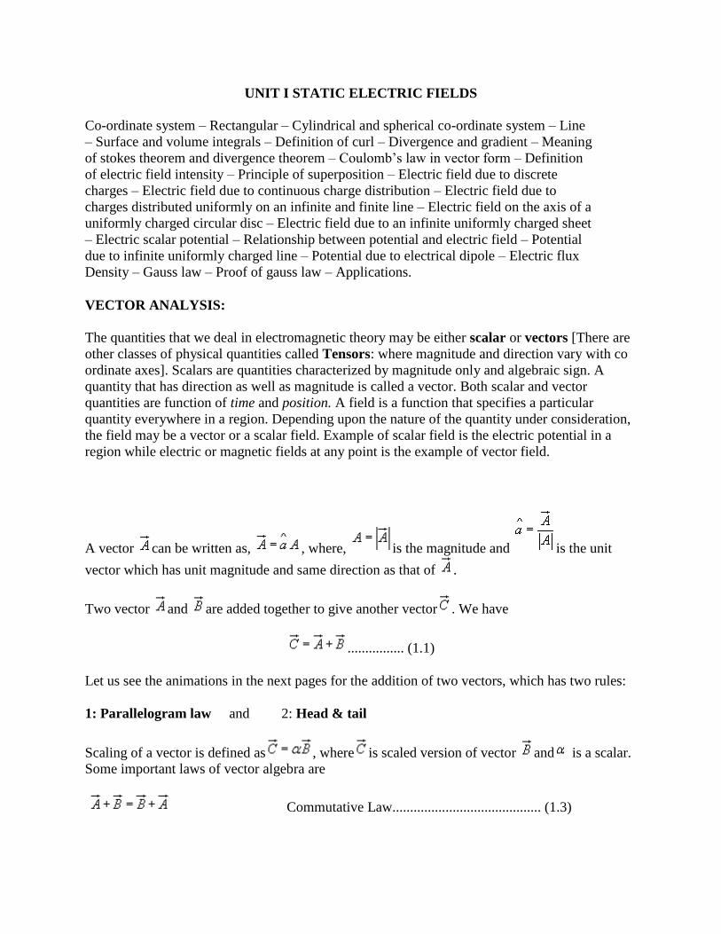
A vector can be written as, , where, is the magnitude and is the unit

vector which has unit magnitude and same direction as that of .

Two vector and are added together to give another vector . We have

................ (1.1)

Let us see the animations in the next pages for the addition of two vectors, which has two rules:

1: Parallelogram law and 2: Head & tail

Scaling of a vector is defined as , where is scaled version of vector and is a scalar.

Some important laws of vector algebra are

Commutative Law.......................................... (1.3)

Associative Law............................................. (1.4)

Distributive Law............................................ (1.5)

The position vector of a point P is the directed distance from the origin (O) to P, i.e., =

.

Fig 1.3: Distance Vector

If = OP and = OQ are the position vectors of the points P and Q then the distance vector

Product of Vectors

When two vectors and are multiplied, the result is either a scalar or a vector depending how the two vectors

were multiplied. The two types of vector multiplication are:

Scalar product (or dot product) gives a scalar.

Vector product (or cross product) gives a vector.

The dot product between two vectors is defined as = |A||B|cosθAB ..................(1.6)

Vector product

is unit vector perpendicular to and

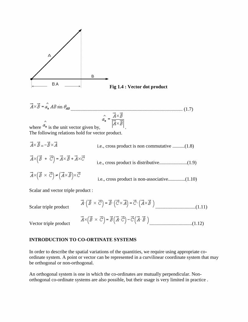
Fig 1.4 : Vector dot product

............................................................................................ (1.7)

where is the unit vector given by, .

The following relations hold for vector product.

= i.e., cross product is non commutative ..........(1.8)

i.e., cross product is distributive.......................(1.9)

i.e., cross product is non-associative..............(1.10)

Scalar and vector triple product :

Scalar triple product .................................(1.11)

Vector triple product ...................................(1.12)

INTRODUCTION TO CO-ORTINATE SYSTEMS

In order to describe the spatial variations of the quantities, we require using appropriate co-

ordinate system. A point or vector can be represented in a curvilinear coordinate system that may

be orthogonal or non-orthogonal.

An orthogonal system is one in which the co-ordinates are mutually perpendicular. Non-

orthogonal co-ordinate systems are also possible, but their usage is very limited in practice .

Let u = constant, v = constant and w = constant represent surfaces in a coordinate system, the

surfaces may be curved surfaces in general. Further, let , and be the unit vectors in the

three coordinate directions(base vectors). In general right handed orthogonal curvilinear systems,

the vectors satisfy the following relations:

..................................... (1.13)

These equations are not independent and specification of one will automatically imply the other

two. Furthermore, the following relations hold

................ (1.14)

A vector can be represented as sum of its orthogonal

components, ................... (1.15)

In general u, v and w may not represent length. We multiply u, v and w by conversion factors

h1,h2 and h3 respectively to convert differential changes du, dv and dw to corresponding changes

in length dl1, dl2, and dl3. Therefore

............... (1.16)

In the same manner, differential volume dv can be written as and differential

area ds1 normal to is given by, . In the same manner, differential areas normal

to unit vectors and can be defined.

In the following sections we discuss three most commonly used orthogonal co-ordinate

systems, viz:

1. Cartesian (or rectangular) co-ordinate system 2. Cylindrical co-ordinate system

3. Spherical polar co-ordinate system

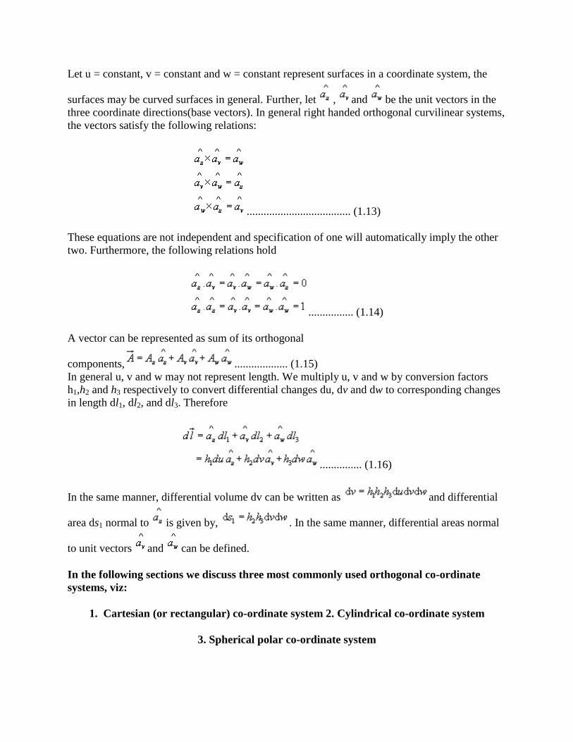
.................... (1.17)

..................... (1.18)

Fig 1.6: Cartesian co-ordinate system

Cartesian Co-ordinate System :

In Cartesian co-ordinate system, we have, (u,v,w) = (x,y,z). A point P(x0, y0, z0) in Cartesian co-ordinate system is

represented as intersection of three planes x = x0, y = y0 and z = z0. The unit vectors satisfies the following relation:

Since x, y and z all represent lengths, h1= h2= h3=1. The differential length, area and volume are defined respectively as

................(1.21)

.................................(1.22)

In cartesian co-ordinate system, a vector can be written as . The dot and cross product of

two vectors and can be written as follows:

.................(1.19)

....................(1.20)

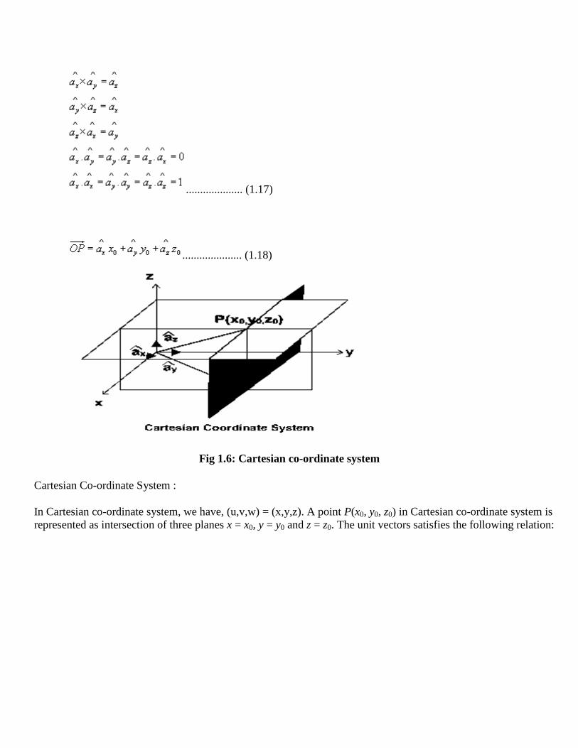
Cylindrical Co-ordinate System :

For cylindrical coordinate systems we have a point is determined as the point of

intersection of a cylindrical surface r = r0, half plane containing the z-axis and making an angle ;

with the xz plane and a plane parallel to xy plane located at z=z0 as shown in figure 7 on next page.

In cylindrical coordinate system, the unit vectors satisfy the following relations

A vector can be written as , ...........................(1.24)

The differential length is defined as,

......................(1.25)

.....................(1.23)

Fig 1.7 : Cylindrical Coordinate System

Differential areas are:

Differential volume,

Fig 1.8 : Differential Volume Element in Cylindrical Coordinates

...............(1.28)

Therefore we can write, ..........(1.29)

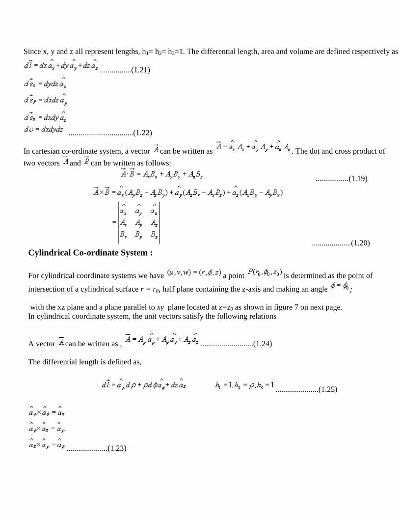
Transformation between Cartesian and Cylindrical coordinates:

Let us consider is to be expressed in Cartesian co-ordinate as . In

doing so we note that and it applies for other components as well.

Fig 1.9 : Unit Vectors in Cartesian and Cylindrical Coordinates

These relations can be put conveniently in the matrix form as:

..................... (1.30)

themselves may be functions of as:

............................ (1.31)

The inverse relationships are: ........................ (1.32)

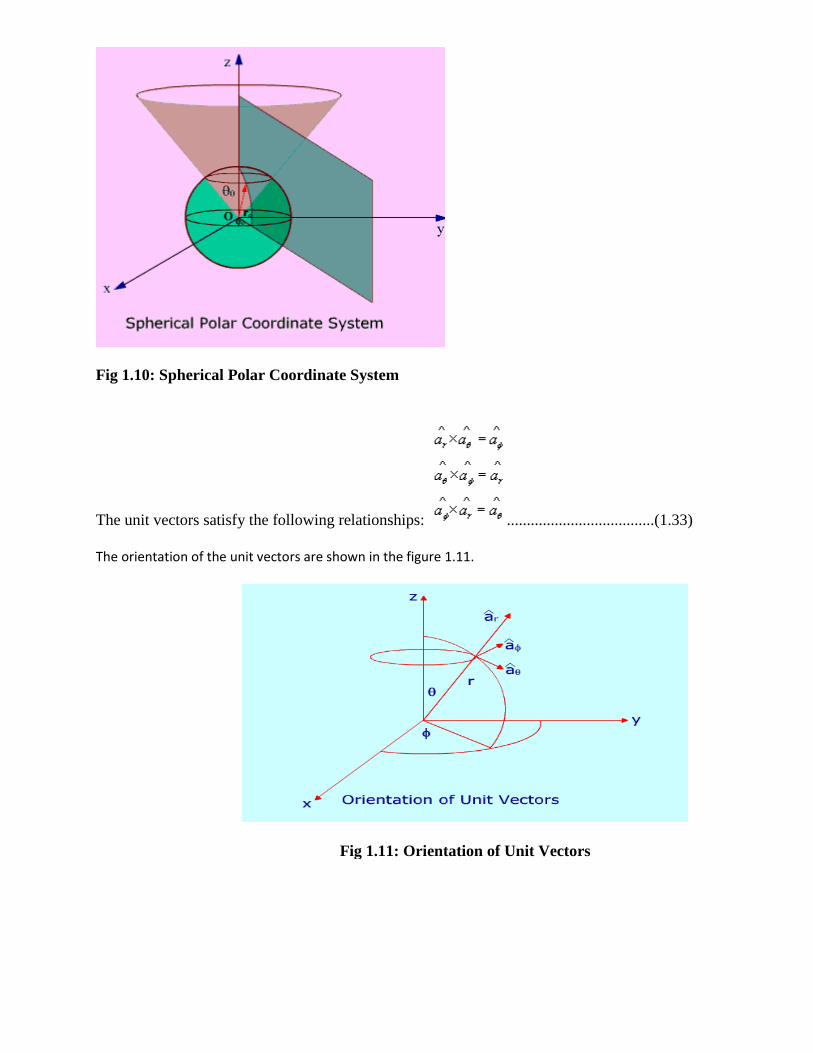
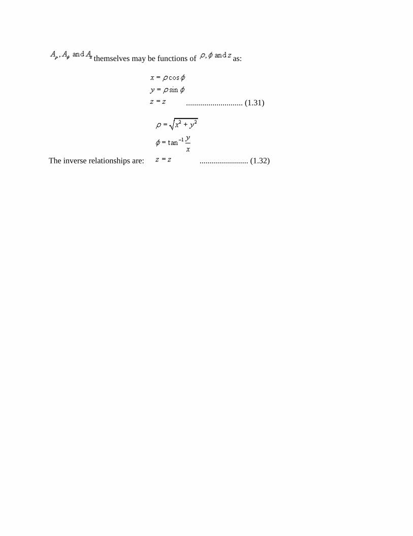
Fig 1.10: Spherical Polar Coordinate System

The unit vectors satisfy the following relationships: .....................................(1.33)

The orientation of the unit vectors are shown in the figure 1.11.

Fig 1.11: Orientation of Unit Vectors

1

INTRODUCTION TO LINE, SURFACE AND VOLUME INTEGRALS :

In electromagnetic theory, we come across integrals, which contain vector functions. Some representative

integrals are listed below:

the above integrals, and respectively represent vector and scalar function of space coordinates. C,S

and V represent path, surface and volume of integration. All these integrals are evaluated using extension

of the usual one-dimensional integral as the limit of a sum, i.e., if a function f(x) is defined over arrange a

to b of values of x, then the integral is given by

.................................(1.42)

where the interval (a,b) is subdivided into n continuous interval of lengths .

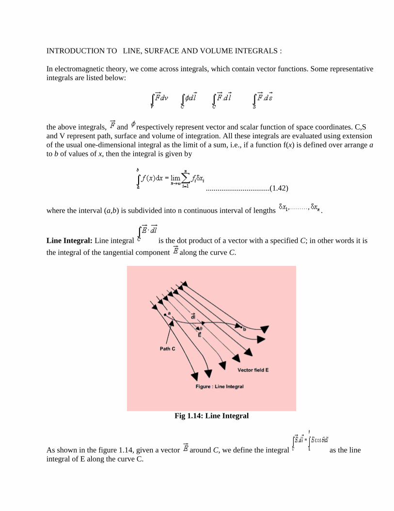
Line Integral: Line integral is the dot product of a vector with a specified C; in other words it is

the integral of the tangential component along the curve C.

Fig 1.14: Line Integral

As shown in the figure 1.14, given a vector around C, we define the integral as the line

integral of E along the curve C.

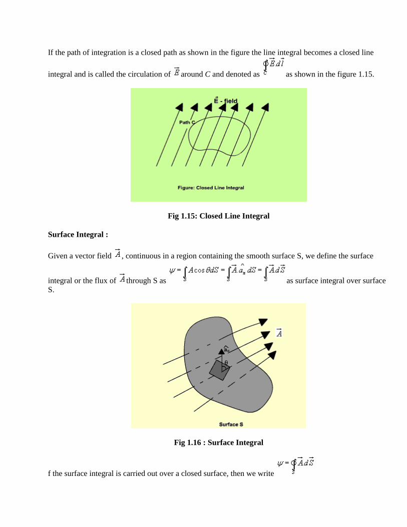
If the path of integration is a closed path as shown in the figure the line integral becomes a closed line

integral and is called the circulation of around C and denoted as as shown in the figure 1.15.

Fig 1.15: Closed Line Integral

Surface Integral :

Given a vector field , continuous in a region containing the smooth surface S, we define the surface

integral or the flux of through S as as surface integral over surface

S.

Fig 1.16 : Surface Integral

f the surface integral is carried out over a closed surface, then we write

v In Cartesian coordinates:

................................................(1.44)

In cylindrical coordinates:

...........................................(1.45)

and in spherical polar coordinates:

.................................(1.46)

Gradient of a Scalar function:

Let us consider a scalar field V(u,v,w) , a function of space coordinates.

Gradient of the scalar field V is a vector that represents both the magnitude and direction of the maximum

space rate of increase of this scalar field V.

volume Integrals:

We define or as the volume integral of the scalar function f(function of spatial coordinates)

over the volume V. Evaluation of integral of the form can be carried out as a sum of three scalar

volume integrals, where each scalar volume integral is a component of the vector

The Del Operator :

The vector differential operator was introduced by Sir W. R. Hamilton and later on developed by P. G.

Tait.

Mathematically the vector differential operator can be written in the general form as:

.................................(1.43)

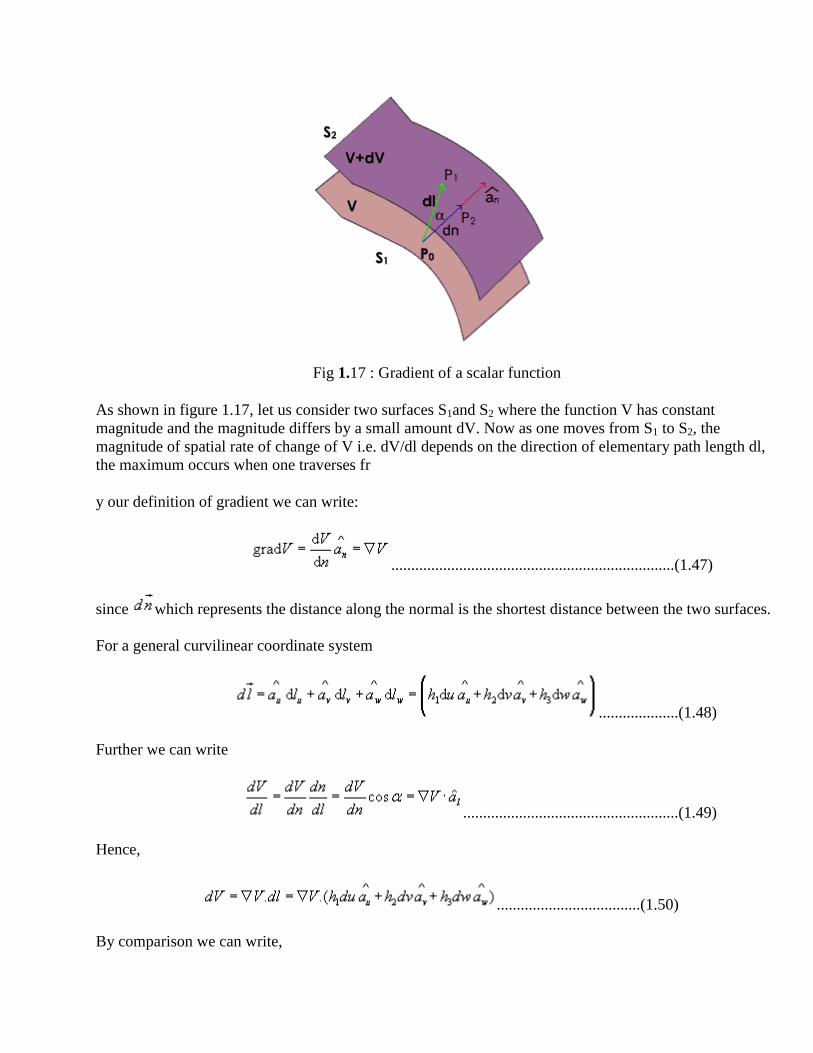
Fig 1.17 : Gradient of a scalar function

As shown in figure 1.17, let us consider two surfaces S1and S2 where the function V has constant

magnitude and the magnitude differs by a small amount dV. Now as one moves from S1 to S2, the

magnitude of spatial rate of change of V i.e. dV/dl depends on the direction of elementary path length dl,

the maximum occurs when one traverses fr

y our definition of gradient we can write:

.......................................................................(1.47)

since which represents the distance along the normal is the shortest distance between the two surfaces.

For a general curvilinear coordinate system

....................(1.48)

Further we can write

......................................................(1.49)

Hence,

....................................(1.50)

By comparison we can write,

....................................................................(1.52)

Hence for the Cartesian, cylindrical and spherical polar coordinate system, the expressions for gradient

can be written as:

In Cartesian coordinates:

...................................................................................(1.53)

Also we can write,

............................(1.51)

n cylindrical coordinates:

..................................................................(1.54)

and in spherical polar coordinates:

..........................................................(1.55)

The following relationships hold for gradient operator.

...............................................................................(1.56)

where U and V are scalar functions and n is an integer.

t may further be noted that since magnitude of depends on the direction of dl, it is called the

directional derivative. If is called the scalar potential function of the vector function .

Divergence of a Vector Field:

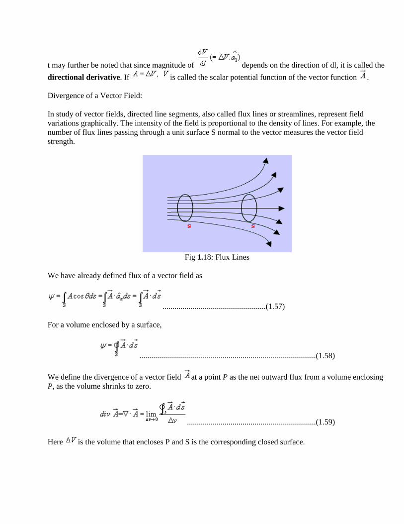
In study of vector fields, directed line segments, also called flux lines or streamlines, represent field

variations graphically. The intensity of the field is proportional to the density of lines. For example, the

number of flux lines passing through a unit surface S normal to the vector measures the vector field

strength.

Fig 1.18: Flux Lines

We have already defined flux of a vector field as

....................................................(1.57)

For a volume enclosed by a surface,

.........................................................................................(1.58)

We define the divergence of a vector field at a point P as the net outward flux from a volume enclosing

P, as the volume shrinks to zero.

.................................................................(1.59)

Here is the volume that encloses P and S is the corresponding closed surface.

Fig 1.19: Evaluation of divergence in curvilinear coordinate

Let us consider a differential volume centered on point P(u,v,w) in a vector field . The flux through an

elementary area normal to u is given by ,

........................................(1.60)

Net outward flux along u can be calculated considering the two elementary surfaces perpendicular to u .

.......................................(1.61)

Considering the contribution from all six surfaces that enclose the volume, we can write

.......................................(1.62)

Hence for the Cartesian, cylindrical and spherical polar coordinate system, the expressions for divergence

can be written as:

In Cartesian coordinates:

................................(1.63)

In cylindrical coordinates:

....................................................................(1.64)

and in spherical polar coordinates:

......................................(1.65)

In connection with the divergence of a vector field, the following can be noted

Divergence of a vector field gives a scalar.

..............................................................................(1.66)

CURL,DIVERGENCE AND GRADIENT

Divergence theorem states that the volume integral of the divergence of vector field is equal to the net

outward flux of the vector through the closed surface that bounds the volume. Mathematically,

Proof:

Let us consider a volume V enclosed by a surface S . Let us subdivide the volume in large number of cells.

Let the kth

cell has a volume and the corresponding surface is denoted by Sk. Interior to the volume,

cells have common surfaces. Outward flux through these common surfaces from one cell becomes the

inward flux for the neighboring cells. Therefore when the total flux from these cells is considered, we

actually get the net outward flux through the surface surrounding the volume. Hence we can write:

......................................(1.67)

In the limit, that is when and the right hand of the expression can be written as

.

Hence we get , which is the divergence theorem.

Curl of a vector field:

We have defined the circulation of a vector field A around a closed path as .

Curl of a vector field is a measure of the vector field's tendency to rotate about a point. Curl , also

written as is defined as a vector whose magnitude is maximum of the net circulation per unit area

when the area tends to zero and its direction is the normal direction to the area when the area is oriented in

such a way so as to make the circulation maximum.

Therefore, we can write:

......................................(1.68)

To derive the expression for curl in generalized curvilinear coordinate system, we first compute f

C1 represents the boundary of , then we can write

......................................(1.69)

The integrals on the RHS can be evaluated as follows:

.................................(1.70)

................................................(1.71)

The negative sign is because of the fact that the direction of traversal reverses. Similarly,

..................................................(1.72)

............................................................................(1.73)

Cartesian coordinates: .......................................(1.78)

In Cylindrical coordinates, ....................................(1.79)

In Spherical polar coordinates, ..............(1.80)

Curl operation exhibits the following properties:

..............(1.81)

Stoke's theorem :

It states that the circulation of a vector field around a closed path is equal to the integral of over

the surface bounded by this path. It may be noted that this equality holds provided and are

continuous on the surface.

i.e,

..............(1.82)

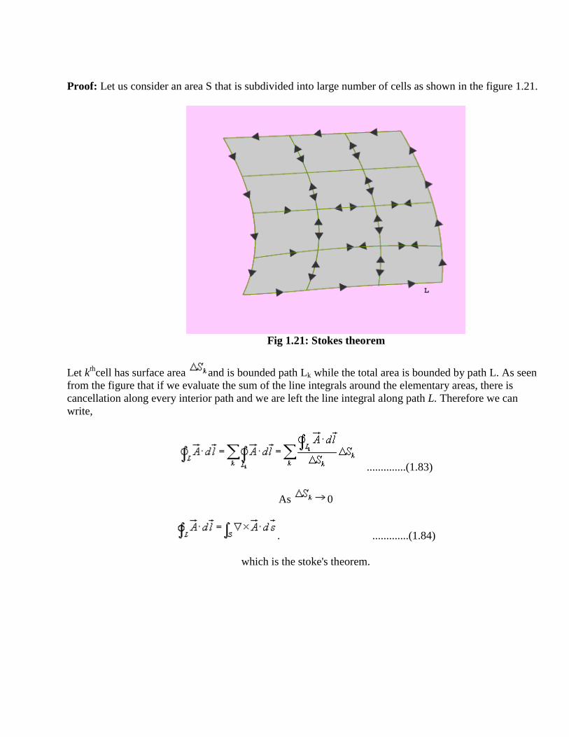
Proof: Let us consider an area S that is subdivided into large number of cells as shown in the figure 1.21.

Fig 1.21: Stokes theorem

Let kth

cell has surface area and is bounded path Lk while the total area is bounded by path L. As seen

from the figure that if we evaluate the sum of the line integrals around the elementary areas, there is

cancellation along every interior path and we are left the line integral along path L. Therefore we can

write,

..............(1.83)

As 0

. .............(1.84)

which is the stoke's theorem.

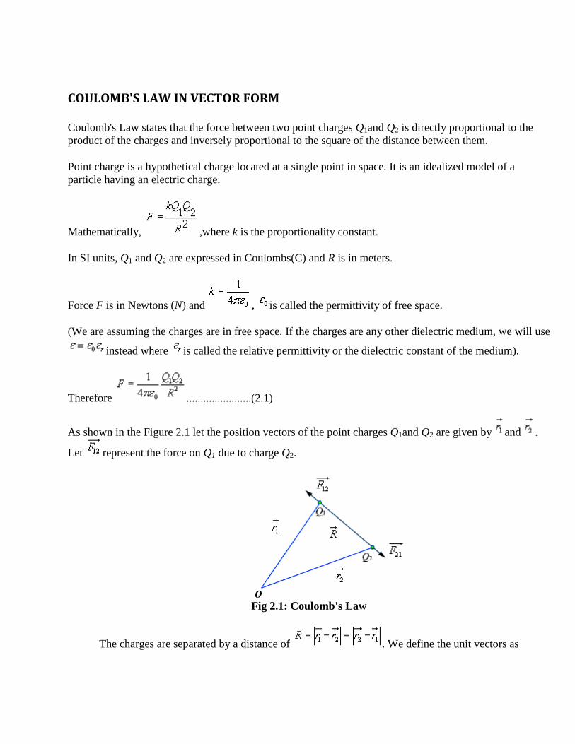
COULOMB'S LAW IN VECTOR FORM

Coulomb's Law states that the force between two point charges Q1and Q2 is directly proportional to the

product of the charges and inversely proportional to the square of the distance between them.

Point charge is a hypothetical charge located at a single point in space. It is an idealized model of a

particle having an electric charge.

Mathematically, ,where k is the proportionality constant.

In SI units, Q1 and Q2 are expressed in Coulombs(C) and R is in meters.

Force F is in Newtons (N) and , is called the permittivity of free space.

(We are assuming the charges are in free space. If the charges are any other dielectric medium, we will use

instead where is called the relative permittivity or the dielectric constant of the medium).

Therefore .......................(2.1)

As shown in the Figure 2.1 let the position vectors of the point charges Q1and Q2 are given by and .

Let represent the force on Q1 due to charge Q2.

Fig 2.1: Coulomb's Law

The charges are separated by a distance of . We define the unit vectors as

and ..................................(2.2)

can be defined as . Similarly the force on Q1 due to charge Q2 can

be calculated and if represents this force then we can write

hen we have a number of point charges, to determine the force on a particular charge due to all other

charges, we apply principle of superposition. If we have N number of charges Q1,Q2,.........QN located

respectively at the points represented by the position vectors , ,...... , the force experienced by a

charge Q located at is given by,

.................................(2.3)

Electric Field

The electric field intensity or the electric field strength at a point is defined as the force per unit charge.

That is

or, .......................................(2.4)

The electric field intensity E at a point r (observation point) due a point charge Q located at (source

point) is given by:

..........................................(2.5)

or a collection of N point charges Q1 ,Q2 ,.........QN located at , ,...... , the electric field intensity at

point is obtained as

........................................(2.6)

The expression (2.6) can be modified suitably to compute the electric filed due to a continuous distribution

of charges.

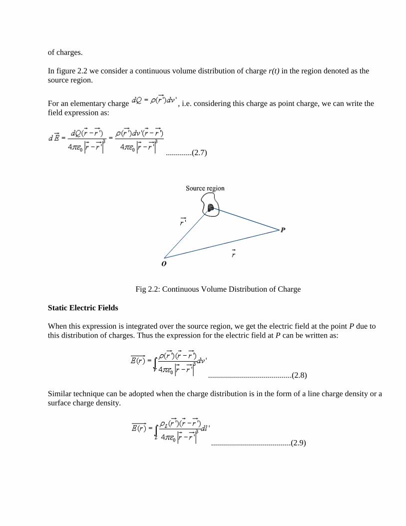
In figure 2.2 we consider a continuous volume distribution of charge r(t) in the region denoted as the

source region.

For an elementary charge , i.e. considering this charge as point charge, we can write the

field expression as:

.............(2.7)

Fig 2.2: Continuous Volume Distribution of Charge

Static Electric Fields

When this expression is integrated over the source region, we get the electric field at the point P due to

this distribution of charges. Thus the expression for the electric field at P can be written as:

..........................................(2.8)

Similar technique can be adopted when the charge distribution is in the form of a line charge density or a

surface charge density.

........................................(2.9)

........................................(2.10)

ELECTRIC FLUX DENSITY:

As stated earlier electric field intensity or simply „Electric field' gives the strength of the field at a

particular point. The electric field depends on the material media in which the field is being considered.

The flux density vector is defined to be independent of the material media (as we'll see that it relates to the

charge that is producing it).For a linear

medium under consideration; the flux density vector is defined as:

................................................(2.11)

We define the electric flux Y as

.....................................(2.12)

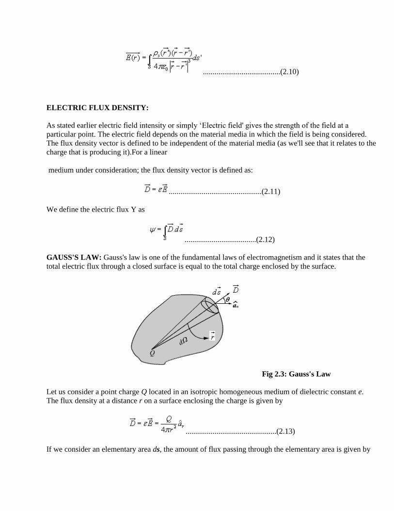
GAUSS'S LAW: Gauss's law is one of the fundamental laws of electromagnetism and it states that the

total electric flux through a closed surface is equal to the total charge enclosed by the surface.

Fig 2.3: Gauss's Law

Let us consider a point charge Q located in an isotropic homogeneous medium of dielectric constant e.

The flux density at a distance r on a surface enclosing the charge is given by

...............................................(2.13)

If we consider an elementary area ds, the amount of flux passing through the elementary area is given by

.....................................(2.14)

But , is the elementary solid angle subtended by the area at the location of Q. Therefore

we can write

For a closed surface enclosing the charge, we can write

which can seen to be same as what we have stated in the definition of Gauss's Law.

APPLICATION OF GAUSS'S LAW

Gauss's law is particularly useful in computing or where the charge distribution has some symmetry.

We shall illustrate the application of Gauss's Law with some examples.

1.AN INFINITE LINE CHARGE

As the first example of illustration of use of Gauss's law, let consider the problem of determination of the

electric field produced by an infinite line charge of density rLC/m. Let us consider a line charge positioned

along the z-axis as shown in Fig. 2.4(a) (next slide). Since the line charge is assumed to be infinitely long,

the electric field will be of the form as shown in Fig. 2.4(b) (next slide).

If we consider a close cylindrical surface as shown in Fig. 2.4(a), using Gauss's theorem we can write,

.....................................(2.15)

Considering the fact that the unit normal vector to areas S1 and S3 are perpendicular to the electric field,

the surface integrals for the top and bottom surfaces evaluates to zero. Hence we can write,

.....................................(2.16)

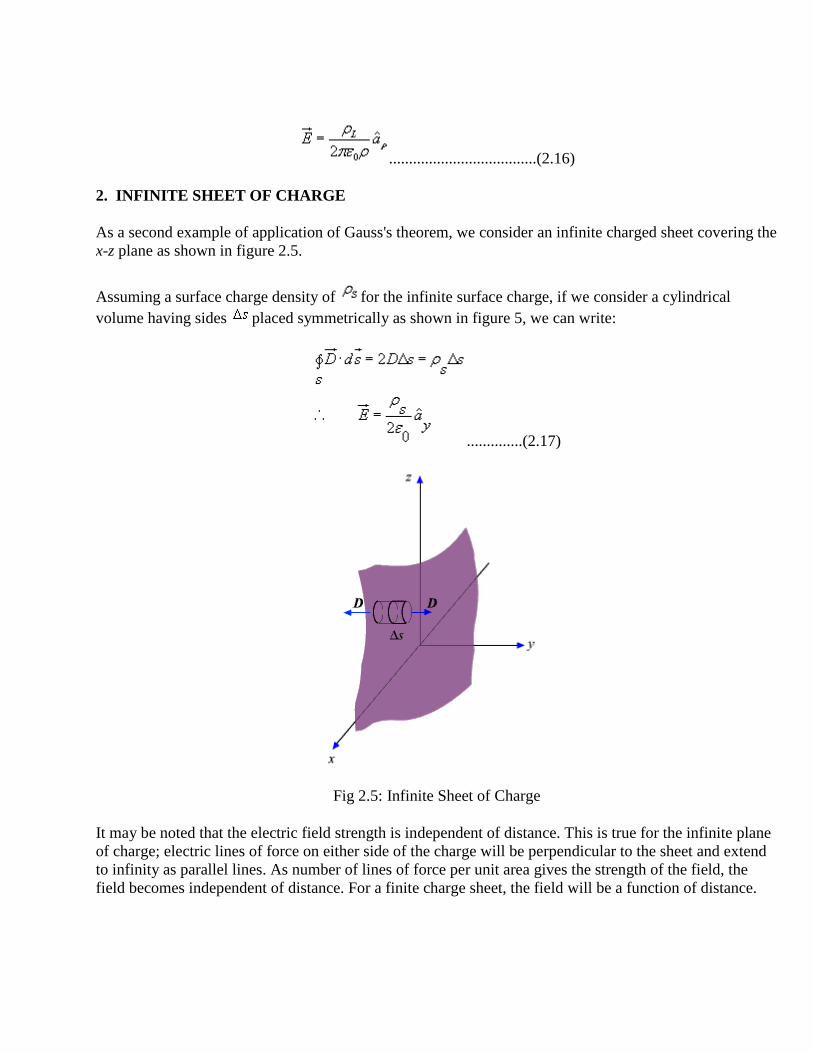
2. INFINITE SHEET OF CHARGE

As a second example of application of Gauss's theorem, we consider an infinite charged sheet covering the

x-z plane as shown in figure 2.5.

Assuming a surface charge density of for the infinite surface charge, if we consider a cylindrical

volume having sides placed symmetrically as shown in figure 5, we can write:

..............(2.17)

Fig 2.5: Infinite Sheet of Charge

It may be noted that the electric field strength is independent of distance. This is true for the infinite plane

of charge; electric lines of force on either side of the charge will be perpendicular to the sheet and extend

to infinity as parallel lines. As number of lines of force per unit area gives the strength of the field, the

field becomes independent of distance. For a finite charge sheet, the field will be a function of distance.

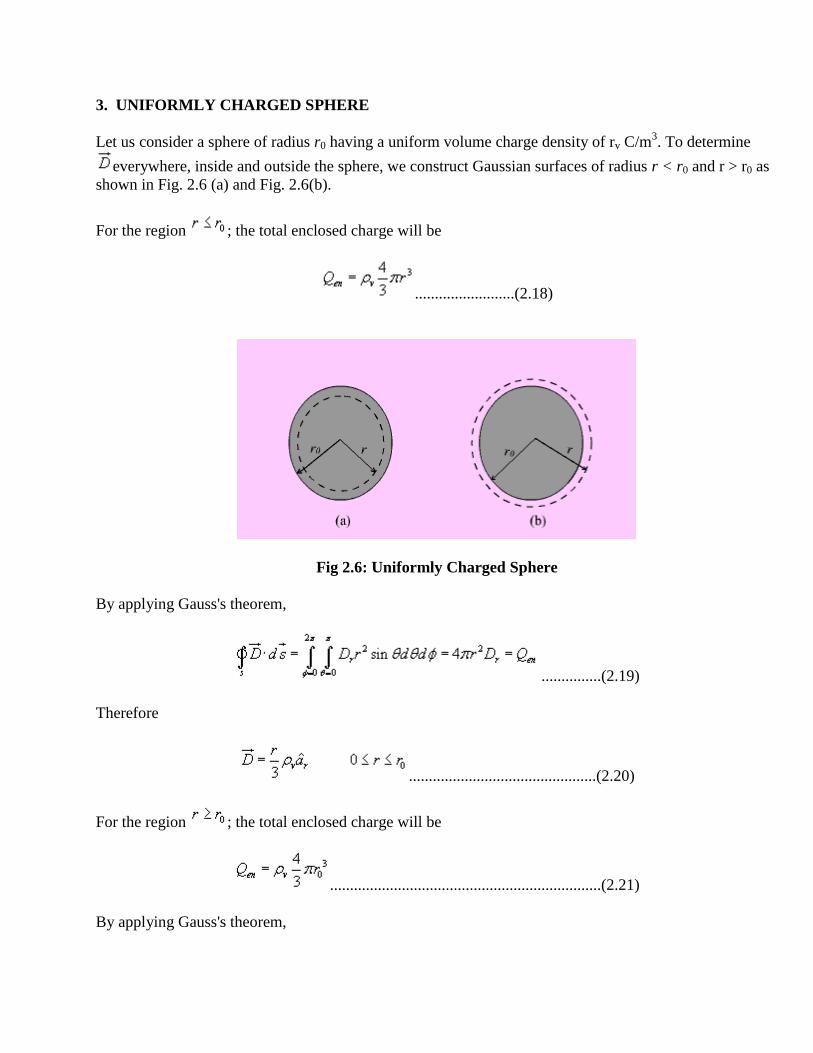
3. UNIFORMLY CHARGED SPHERE

Let us consider a sphere of radius r0 having a uniform volume charge density of rv C/m3. To determine

everywhere, inside and outside the sphere, we construct Gaussian surfaces of radius r < r0 and r > r0 as

shown in Fig. 2.6 (a) and Fig. 2.6(b).

For the region ; the total enclosed charge will be

.........................(2.18)

Fig 2.6: Uniformly Charged Sphere

By applying Gauss's theorem,

...............(2.19)

Therefore

...............................................(2.20)

For the region ; the total enclosed charge will be

....................................................................(2.21)

By applying Gauss's theorem,

.....................................................(2.22)

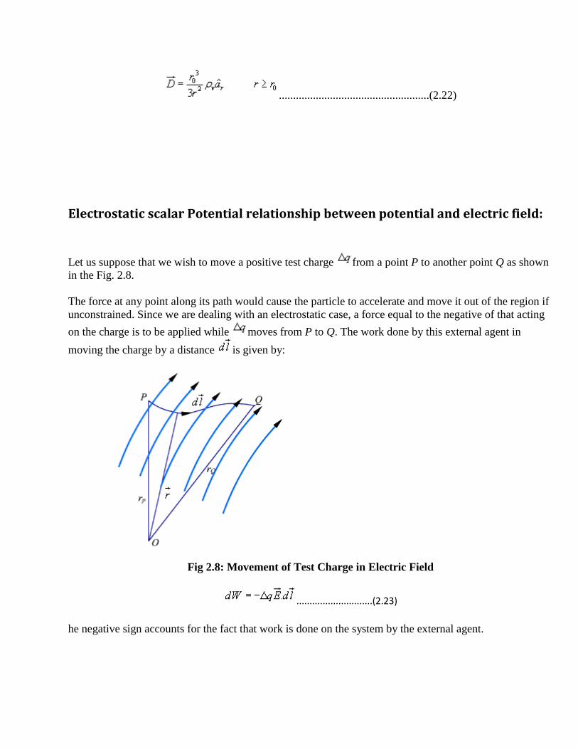
Electrostatic scalar Potential relationship between potential and electric field:

Let us suppose that we wish to move a positive test charge from a point P to another point Q as shown

in the Fig. 2.8.

The force at any point along its path would cause the particle to accelerate and move it out of the region if

unconstrained. Since we are dealing with an electrostatic case, a force equal to the negative of that acting

on the charge is to be applied while moves from P to Q. The work done by this external agent in

moving the charge by a distance is given by:

Fig 2.8: Movement of Test Charge in Electric Field

.............................(2.23)

he negative sign accounts for the fact that work is done on the system by the external agent.

.....................................(2.24)

The potential difference between two points P and Q , VPQ, is defined as the work done per unit charge,

i.e.

...............................(2.25)

It may be noted that in moving a charge from the initial point to the final point if the potential difference is

positive, there is a gain in potential energy in the movement, external agent performs the work against the

field. If the sign of the potential difference is negative, work is done by the field.

We will see that the electrostatic system is conservative in that no net energy is exchanged if the test

charge is moved about a closed path, i.e. returning to its initial position. Further, the potential difference

between two points in an electrostatic field is a point function; it is independent of the path taken. The

potential difference is measured in Joules/Coulomb which is referred to as Volts.

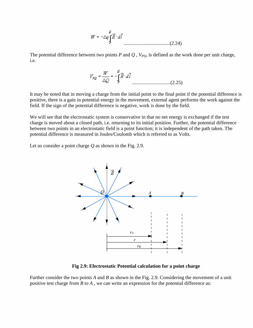
Let us consider a point charge Q as shown in the Fig. 2.9.

Fig 2.9: Electrostatic Potential calculation for a point charge

Further consider the two points A and B as shown in the Fig. 2.9. Considering the movement of a unit

positive test charge from B to A , we can write an expression for the potential difference as:

..................................(2.26)

It is customary to choose the potential to be zero at infinity. Thus potential at any point ( rA = r) due to a

point charge Q can be written as the amount of work done in bringing a unit positive charge from infinity

to that point (i.e. rB = 0).

..................................(2.27)

Or, in other words,

..................................(2.28)

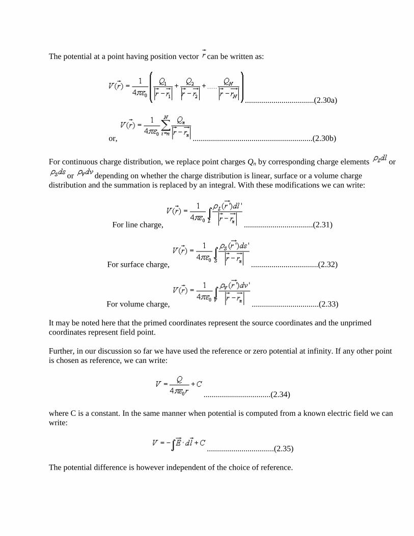
Let us now consider a situation where the point charge Q is not located at the origin as shown in Fig. 2.10.

Fig 2.10: Electrostatic Potential due a Displaced Charge

The potential at a point P becomes

..................................(2.29)

o far we have considered the potential due to point charges only. As any other type of charge distribution

can be considered to be consisting of point charges, the same basic ideas now can be extended to other

types of charge distribution also.

Let us first consider N point charges Q1, Q2,.....QN located at points with position vectors , ,...... .

The potential at a point having position vector can be written as:

..................................(2.30a)

or, ...........................................................(2.30b)

For continuous charge distribution, we replace point charges Qn by corresponding charge elements or

or depending on whether the charge distribution is linear, surface or a volume charge

distribution and the summation is replaced by an integral. With these modifications we can write:

For line charge, ..................................(2.31)

For surface charge, .................................(2.32)

For volume charge, .................................(2.33)

It may be noted here that the primed coordinates represent the source coordinates and the unprimed

coordinates represent field point.

Further, in our discussion so far we have used the reference or zero potential at infinity. If any other point

is chosen as reference, we can write:

.................................(2.34)

where C is a constant. In the same manner when potential is computed from a known electric field we can

write:

.................................(2.35)

The potential difference is however independent of the choice of reference.

.......................(2.36)

We have mentioned that electrostatic field is a conservative field; the work done in moving a charge from

one point to the other is independent of the path. Let us consider moving a charge from point P1 to P2 in

one path and then from point P2 back to P1 over a different path. If the work done on the two paths were

different, a net positive or negative amount of work would have been done when the body returns to its

original position P1. In a conservative field there is no mechanism for dissipating energy corresponding to

any positive work neither any source is present from which energy could be absorbed in the case of

negative work. Hence the question of different works in two paths is untenable, the work must have to be

independent of path and depends on the initial and final positions.

Since the potential difference is independent of the paths taken, VAB = - VBA , and over a closed path,

.................................(2.37)

Applying Stokes's theorem, we can write:

............................(2.38)

from which it follows that for electrostatic field,

........................................(2.39)

Any vector field that satisfies is called an irrotational field.

From our definition of potential, we can write

.................................(2.40)

from which we obtain,

..........................................(2.41)

components of are interrelated by the relation .

When r1 and r2>>d, we can write and .

Therefore,

....................................................(2.43)

We can write,

...............................................(2.44)

The quantity is called the dipole moment of the electric dipole.

Hence the expression for the electric potential can now be written as:

................................(2.45)

It may be noted that while potential of an isolated charge varies with distance as 1/r that of an electric

dipole varies as 1/r2 with distance.

If the dipole is not centered at the origin, but the dipole center lies at , the expression for the potential

can be written as:

........................(2.46)

he electric field for the dipole centered at the origin can be computed as

........................(2.47)

is the magnitude of the dipole moment. Once again we note that the electric field of electric dipole

varies as 1/r3 where as that of a point charge varies as 1/r

2.

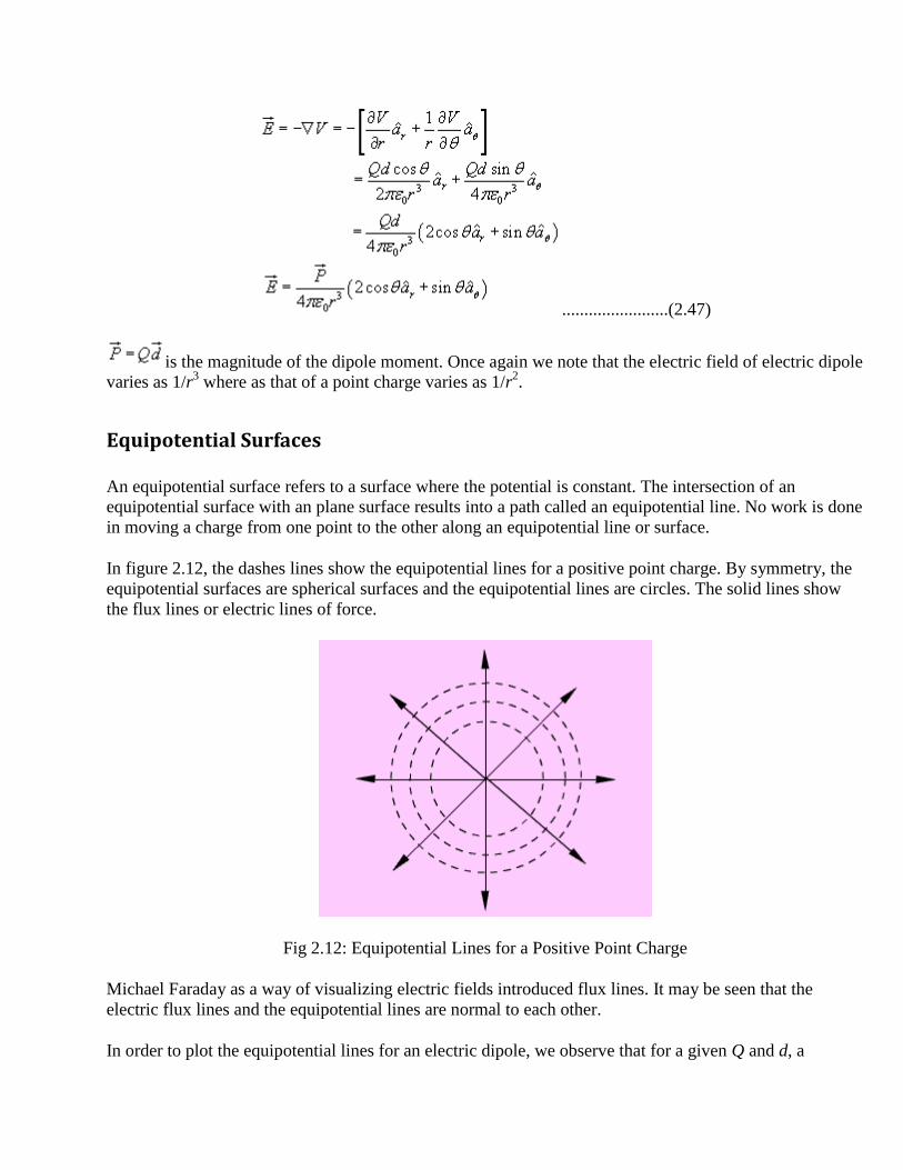
Equipotential Surfaces

An equipotential surface refers to a surface where the potential is constant. The intersection of an

equipotential surface with an plane surface results into a path called an equipotential line. No work is done

in moving a charge from one point to the other along an equipotential line or surface.

In figure 2.12, the dashes lines show the equipotential lines for a positive point charge. By symmetry, the

equipotential surfaces are spherical surfaces and the equipotential lines are circles. The solid lines show

the flux lines or electric lines of force.

Fig 2.12: Equipotential Lines for a Positive Point Charge

Michael Faraday as a way of visualizing electric fields introduced flux lines. It may be seen that the

electric flux lines and the equipotential lines are normal to each other.

In order to plot the equipotential lines for an electric dipole, we observe that for a given Q and d, a

constant V requires that is a constant. From this we can write to be the equation for an

equipotential surface and a family of surfaces can be generated for various values of cv.When plotted in 2-

D this would give equipotential lines.

To determine the equation for the electric field lines, we note that field lines represent the direction of in

space. Therefore,

, k is a constant .................................................................(2.48)

.................(2.49)

For the dipole under consideration =0 , and therefore we can write,

.........................................................(2.50)

BOUNDARY CONDITIONS FOR ELECTROSTATIC FIELDS

In our discussions so far we have considered the existence of electric field in the homogeneous medium.

Practical electromagnetic problems often involve media with different physical properties. Determination

of electric field for such problems requires the knowledge of the relations of field quantities at an interface

between two media. The conditions that the fields must satisfy at the interface of two different media are

referred to as boundary conditions .

In order to discuss the boundary conditions, we first consider the field behavior in some common material

media.

In general, based on the electric properties, materials can be classified into three categories: conductors,

semiconductors and insulators (dielectrics). In conductor , electrons in the outermost shells of the atoms

are very loosely held and they migrate easily from one atom to the other. Most metals belong to this

group. The electrons in the atoms of insulators or dielectrics remain confined to their orbits and under

normal circumstances they are not liberated under the influence of an externally applied field. The

electrical properties of semiconductors fall between those of conductors and insulators since

semiconductors have very few numbers of free charges.

The parameter conductivity is used characterizes the macroscopic electrical property of a material

medium. The notion of conductivity is more important in dealing with the current flow and hence the

same will be considered in detail later on.

If some free charge is introduced inside a conductor, the charges will experience a force due to mutual

repulsion and owing to the fact that they are free to move, the charges will appear on the surface. The

charges will redistribute themselves in such a manner that the field within the conductor is zero.

Therefore, under steady condition, inside a conductor .

From Gauss's theorem it follows that

= 0 .......................(2.51)

The surface charge distribution on a conductor depends on the shape of the conductor. The charges on the

surface of the conductor will not be in equilibrium if there is a tangential component of the electric field is

present, which would produce movement of the charges. Hence under static field conditions, tangential

component of the electric field on the conductor surface is zero. The electric field on the surface of the

conductor is normal everywhere to the surface . Since the tangential component of electric field is zero,

the conductor surface is an equipotential surface. As = 0 inside the conductor, the conductor as a whole

has the same potential. We may further note that charges require a finite time to redistribute in a

conductor. However, this time is very small sec for good conductor like copper.

Let us now consider an interface between a conductor and free space as shown in the figure 2.14.

Fig 2.14: Boundary Conditions for at the surface of a Conductor

Let us consider the closed path pqrsp for which we can write,

.................................(2.52)

For and noting that inside the conductor is zero, we can write

=0.......................................(2.53)

Et is the tangential component of the field. Therefore we find that

Et = 0 ...........................................(2.54)

In order to determine the normal component En, the normal component of , at the surface of the

conductor, we consider a small cylindrical Gaussian surface as shown in the Fig.12. Let represent the

area of the top and bottom faces and represents the height of the cylinder. Once again, as , we

approach the surface of the conductor. Since = 0 inside the conductor is zero,

.............(2.55)

..................(2.56)

Therefore, we can summarize the boundary conditions at the surface of a conductor as:

Et = 0 ........................(2.57)

.....................(2.58)

Behavior of dielectrics in static electric field: Polarization of dielectric

Here we briefly describe the behavior of dielectrics or insulators when placed in static electric field. Ideal

dielectrics do not contain free charges. As we know, all material media are composed of atoms where a

positively charged nucleus (diameter ~ 10-15

m) is surrounded by negatively charged electrons (electron

cloud has radius ~ 10-10

m) moving around the nucleus. Molecules of dielectrics are neutral

macroscopically; an externally applied field causes small displacement of the charge particles creating

small electric dipoles.These induced dipole moments modify electric fields both inside and outside

dielectric material.

being the number of molecules per unit volume i.e. is the dipole moment per unit volume. Let us now

consider a dielectric material having polarization and compute the potential at an external point O due

to an elementary dipole dv'.

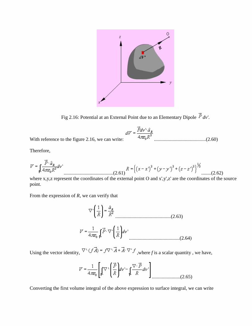
Fig 2.16: Potential at an External Point due to an Elementary Dipole dv'.

With reference to the figure 2.16, we can write: ..........................................(2.60)

Therefore,

........................................(2.61) ........(2.62)

where x,y,z represent the coordinates of the external point O and x',y',z' are the coordinates of the source

point.

From the expression of R, we can verify that

.............................................(2.63)

.........................................(2.64)

Using the vector identity, ,where f is a scalar quantity , we have,

.......................(2.65)

Converting the first volume integral of the above expression to surface integral, we can write

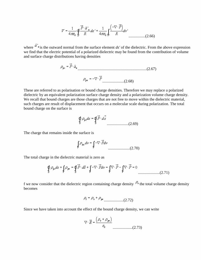
.................(2.66)

where is the outward normal from the surface element ds' of the dielectric. From the above expression

we find that the electric potential of a polarized dielectric may be found from the contribution of volume

and surface charge distributions having densities

......................................................................(2.67)

......................(2.68)

These are referred to as polarisation or bound charge densities. Therefore we may replace a polarized

dielectric by an equivalent polarization surface charge density and a polarization volume charge density.

We recall that bound charges are those charges that are not free to move within the dielectric material,

such charges are result of displacement that occurs on a molecular scale during polarization. The total

bound charge on the surface is

......................(2.69)

The charge that remains inside the surface is

......................(2.70)

The total charge in the dielectric material is zero as

......................(2.71)

f we now consider that the dielectric region containing charge density the total volume charge density

becomes

....................(2.72)

Since we have taken into account the effect of the bound charge density, we can write

....................(2.73)

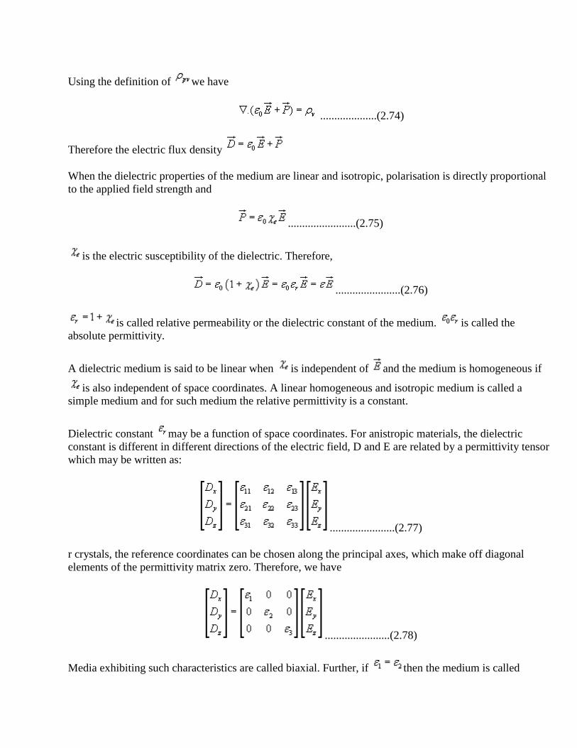
Using the definition of we have

....................(2.74)

Therefore the electric flux density

When the dielectric properties of the medium are linear and isotropic, polarisation is directly proportional

to the applied field strength and

........................(2.75)

is the electric susceptibility of the dielectric. Therefore,

.......................(2.76)

is called relative permeability or the dielectric constant of the medium. is called the

absolute permittivity.

A dielectric medium is said to be linear when is independent of and the medium is homogeneous if

is also independent of space coordinates. A linear homogeneous and isotropic medium is called a

simple medium and for such medium the relative permittivity is a constant.

Dielectric constant may be a function of space coordinates. For anistropic materials, the dielectric

constant is different in different directions of the electric field, D and E are related by a permittivity tensor

which may be written as:

.......................(2.77)

r crystals, the reference coordinates can be chosen along the principal axes, which make off diagonal

elements of the permittivity matrix zero. Therefore, we have

.......................(2.78)

Media exhibiting such characteristics are called biaxial. Further, if then the medium is called

uniaxial. It may be noted that for isotropic media, .

Lossy dielectric materials are represented by a complex dielectric constant, the imaginary part of which

provides the power loss in the medium and this is in general dependent on frequency.

Another phenomenon is of importance is dielectric breakdown. We observed that the applied electric field

causes small displacement of bound charges in a dielectric material that result into polarization. Strong

field can pull electrons completely out of the molecules. These electrons being accelerated under influence

of electric field will collide with molecular lattice structure causing damage or distortion of material. For

very strong fields, avalanche breakdown may also occur. The dielectric under such condition will become

conducting.

The maximum electric field intensity a dielectric can withstand without breakdown is referred to as the

dielectric strength of the material.

BOUNDARY CONDITIONS FOR ELECTROSTATIC FIELDS:

Let us consider the relationship among the field components that exist at the interface between two

dielectrics as shown in the figure 2.17. The permittivity of the medium 1 and medium 2 are and

respectively and the interface may also have a net charge density Coulomb/m.

Fig 2.17: Boundary Conditions at the interface between two dielectrics

We can express the electric field in terms of the tangential and normal

components ..........(2.79)

here Et and En are the tangential and normal components of the electric field respectively.

Let us assume that the closed path is very small so that over the elemental path length the variation of E

can be neglected. Moreover very near to the interface, . Therefore

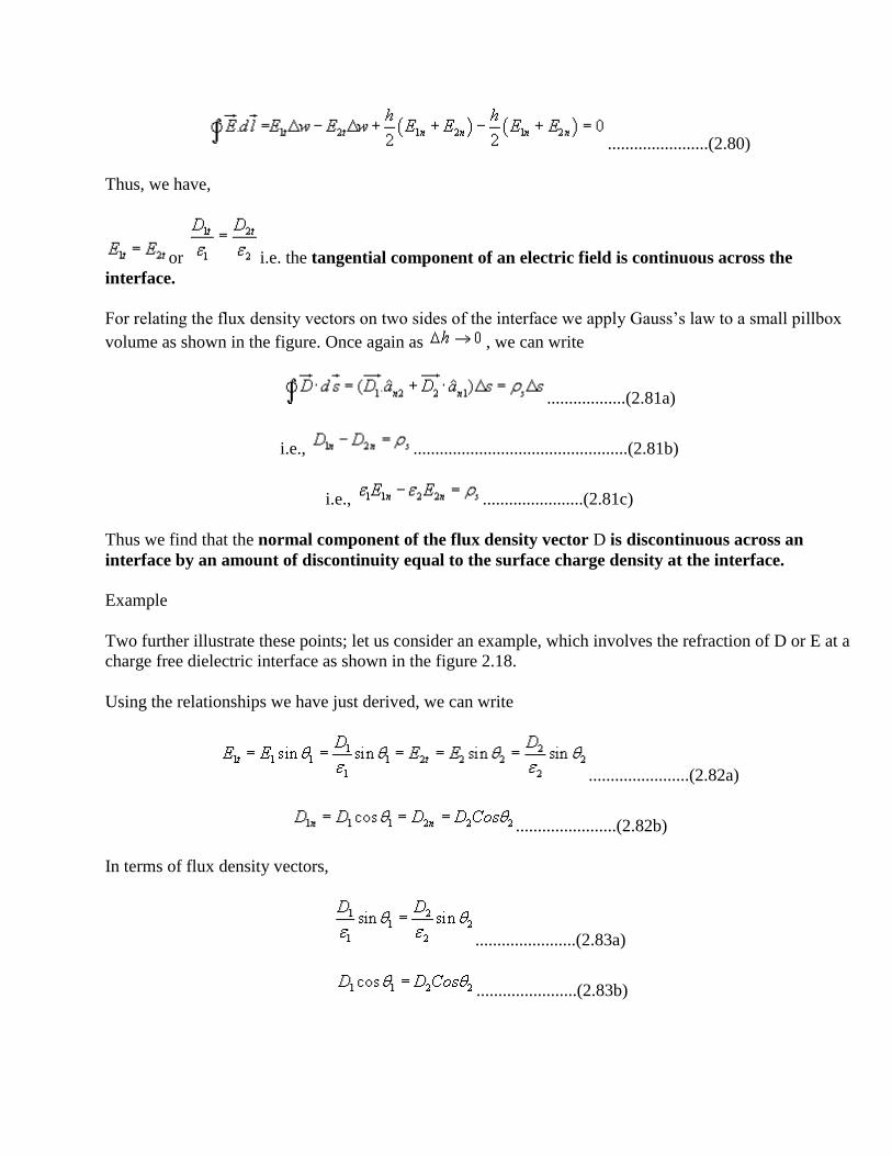
.......................(2.80)

Thus, we have,

or i.e. the tangential component of an electric field is continuous across the

interface.

For relating the flux density vectors on two sides of the interface we apply Gauss‟s law to a small pillbox

volume as shown in the figure. Once again as , we can write

..................(2.81a)

i.e., .................................................(2.81b)

i.e., .......................(2.81c)

Thus we find that the normal component of the flux density vector D is discontinuous across an

interface by an amount of discontinuity equal to the surface charge density at the interface.

Example

Two further illustrate these points; let us consider an example, which involves the refraction of D or E at a

charge free dielectric interface as shown in the figure 2.18.

Using the relationships we have just derived, we can write

.......................(2.82a)

.......................(2.82b)

In terms of flux density vectors,

.......................(2.83a)

.......................(2.83b)

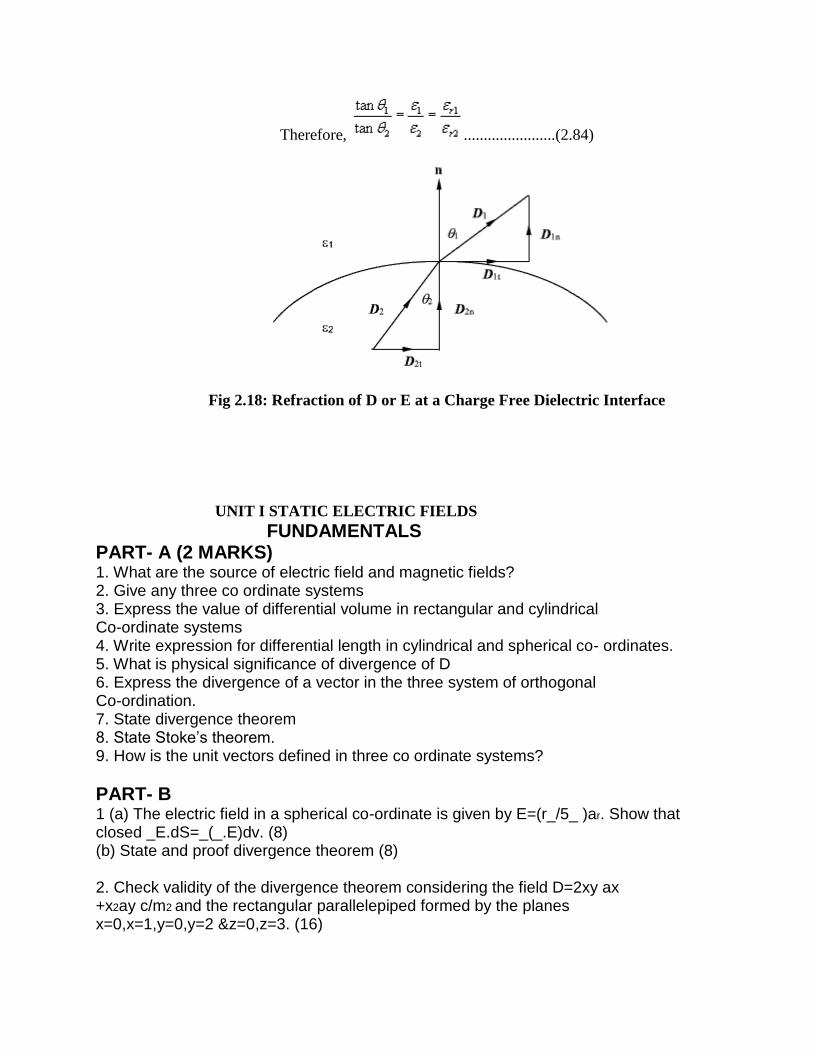
Therefore, .......................(2.84)

Fig 2.18: Refraction of D or E at a Charge Free Dielectric Interface

UNIT I STATIC ELECTRIC FIELDS FUNDAMENTALS PART- A (2 MARKS) 1. What are the source of electric field and magnetic fields? 2. Give any three co ordinate systems 3. Express the value of differential volume in rectangular and cylindrical Co-ordinate systems 4. Write expression for differential length in cylindrical and spherical co- ordinates. 5. What is physical significance of divergence of D 6. Express the divergence of a vector in the three system of orthogonal Co-ordination. 7. State divergence theorem 8. State Stoke’s theorem. 9. How is the unit vectors defined in three co ordinate systems?

PART- B 1 (a) The electric field in a spherical co-ordinate is given by E=(r_/5_ )ar. Show that closed _E.dS=_(_.E)dv. (8) (b) State and proof divergence theorem (8) 2. Check validity of the divergence theorem considering the field D=2xy ax +x2ay c/m2 and the rectangular parallelepiped formed by the planes x=0,x=1,y=0,y=2 &z=0,z=3. (16)

3. A vector field D=[5r2/4]Ir is given in spherical co-ordinates. Evaluate both sides of divergence theorem for the volume enclosed between r=1&r=2. (16) 4. Given A= 2r cos_Ir+rI_ in cylindrical co-ordinates .for the contour x=0 to1 y=0 to1 , verify stoke’s theorem (16) 5. Explain three co-ordinate system. (16) 6. Determine the divergence of these vector fields i. P=x2yz ax+xy az

ii. Q=_sin_ a_+_2z a_+zcos_ az

iii. T=(1/r2)cos_ ar + r sin_cos_ a_ + cos_ a_ (16) 7. (a) Discuss about curl of a vector (6) (b) Derive an expression for curl of a vector (7) (c) State stoke’s theorem (3) 8. (a) Define divergence, gradient, curl in spherical co-ordinate system with mathematical expression (8)

(b) Prove that divergence of a curl of a vector is zero ,using stoke’s theorem (8)

UNIT II STATIC MAGNETIC FIELD

The biot-savart law in vector form – Magnetic field intensity due to a finite and infinite

wire carrying a current I – Magnetic field intensity on the axis of a circular and

rectangular loop carrying a current I – Ampere‟s circuital law and simple applications –

Magnetic flux density – The lorentz force equation for a moving charge and applications

– Force on a wire carrying a current I placed in a magnetic field – Torque on a loop

carrying a current I – Magnetic moment – Magnetic vector potential.

The source of steady magnetic field may be a permanent magnet, a direct current or an electric field

changing with time. In this chapter we shall mainly consider the magnetic field produced by a direct

current. The magnetic field produced due to time varying electric field will be discussed later.

Historically, the link between the electric and magnetic field was established Oersted in 1820. Ampere and

others extended the investigation of magnetic effect of electricity. There are two major laws governing the

magnetostatic fields are:

Biot-Savart Law

Ampere's Law

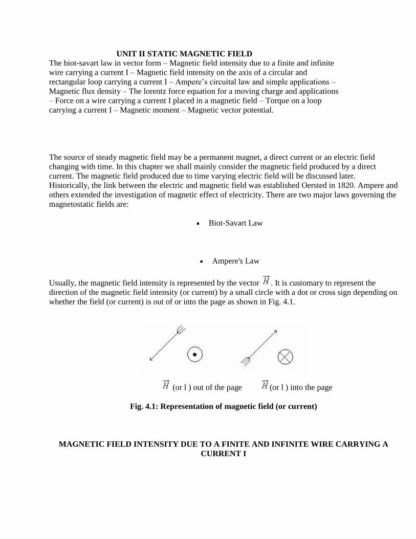
Usually, the magnetic field intensity is represented by the vector . It is customary to represent the

direction of the magnetic field intensity (or current) by a small circle with a dot or cross sign depending on

whether the field (or current) is out of or into the page as shown in Fig. 4.1.

(or l ) out of the page (or l ) into the page

Fig. 4.1: Representation of magnetic field (or current)

MAGNETIC FIELD INTENSITY DUE TO A FINITE AND INFINITE WIRE CARRYING A

CURRENT I

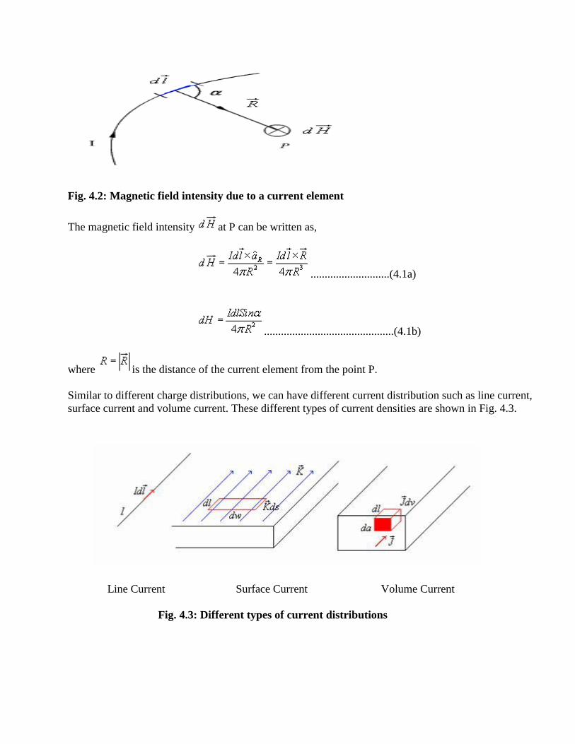
Fig. 4.2: Magnetic field intensity due to a current element

The magnetic field intensity at P can be written as,

............................(4.1a)

..............................................(4.1b)

where is the distance of the current element from the point P.

Similar to different charge distributions, we can have different current distribution such as line current,

surface current and volume current. These different types of current densities are shown in Fig. 4.3.

Line Current Surface Current Volume Current

Fig. 4.3: Different types of current distributions

By denoting the surface current density as K (in amp/m) and volume current density as J (in amp/m2) we can write:

......................................(4.2)

( It may be noted that )

Employing Biot-Savart Law, we can now express the magnetic field intensity H. In terms of these current

distributions.

............................. for line current............................(4.3a)

........................ for surface current ....................(4.3b)

....................... for volume current......................(4.3c)

Fig. 4.4: Field at a point P due to a finite length current carrying conductor

To illustrate the application of Biot - Savart's Law, we consider the following example.

Example 4.1: We consider a finite length of a conductor carrying a current placed along z-axis as shown in the

Fig 4.4. We determine the magnetic field at point P due to this current carrying conductor.

With reference to Fig. 4.4, we find that

.......................................................(4.4)

Applying Biot - Savart's law for the current element

we can write,

........................................................(4.5)

Substituting we can write,

.........................(4.6)

We find that, for an infinitely long conductor carrying a current I , and

Therefore, .........................................................................................(4.7)

AMPERE'S CIRCUITAL LAW:

Ampere's circuital law states that the line integral of the magnetic field (circulation of H ) around a

closed path is the net current enclosed by this path. Mathematically,

......................................(4.8)

The total current I enc can be written as,

...................................... (4.9)

By applying Stoke's theorem, we can write

......................................(4.10)

which is the Ampere's law in the point form.

Applications of Ampere's law:

We illustrate the application of Ampere's Law with some examples.

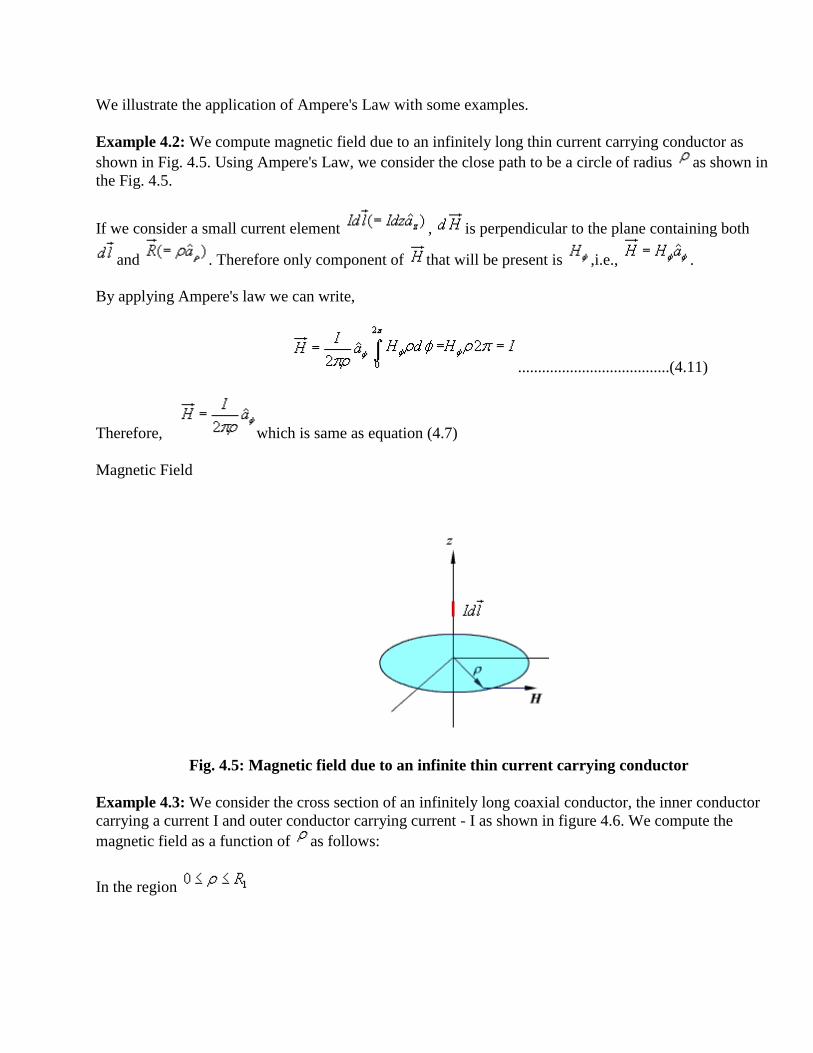
Example 4.2: We compute magnetic field due to an infinitely long thin current carrying conductor as

shown in Fig. 4.5. Using Ampere's Law, we consider the close path to be a circle of radius as shown in

the Fig. 4.5.

If we consider a small current element , is perpendicular to the plane containing both

and . Therefore only component of that will be present is ,i.e., .

By applying Ampere's law we can write,

......................................(4.11)

Therefore, which is same as equation (4.7)

Magnetic Field

Fig. 4.5: Magnetic field due to an infinite thin current carrying conductor

Example 4.3: We consider the cross section of an infinitely long coaxial conductor, the inner conductor

carrying a current I and outer conductor carrying current - I as shown in figure 4.6. We compute the

magnetic field as a function of as follows:

In the region

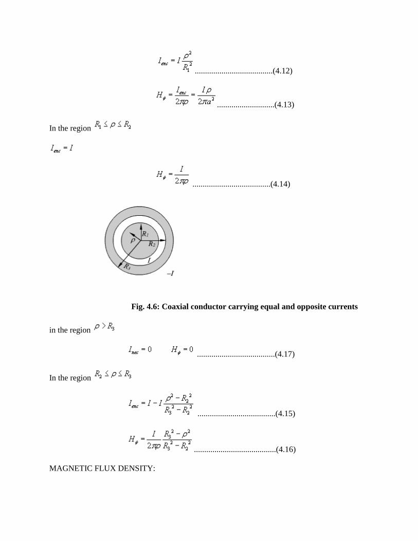
......................................(4.12)

............................(4.13)

In the region

......................................(4.14)

Fig. 4.6: Coaxial conductor carrying equal and opposite currents

in the region

......................................(4.17)

In the region

......................................(4.15)

........................................(4.16)

MAGNETIC FLUX DENSITY:

In simple matter, the magnetic flux density related to the magnetic field intensity as where called

the permeability. In particular when we consider the free space where H/m is the

permeability of the free space. Magnetic flux density is measured in terms of Wb/m 2 .

The magnetic flux density through a surface is given by:

Wb ......................................(4.18)

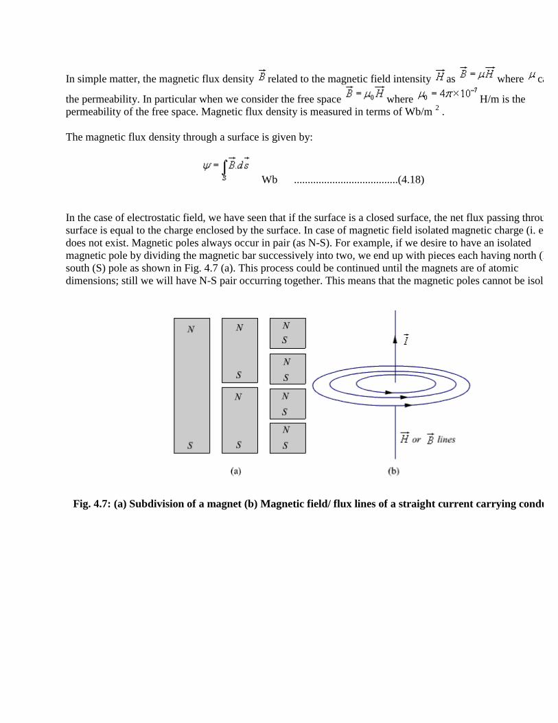
In the case of electrostatic field, we have seen that if the surface is a closed surface, the net flux passing through the

surface is equal to the charge enclosed by the surface. In case of magnetic field isolated magnetic charge (i. e. pole)

does not exist. Magnetic poles always occur in pair (as N-S). For example, if we desire to have an isolated

magnetic pole by dividing the magnetic bar successively into two, we end up with pieces each having north (N) and

south (S) pole as shown in Fig. 4.7 (a). This process could be continued until the magnets are of atomic

dimensions; still we will have N-S pair occurring together. This means that the magnetic poles cannot be isolated.

Fig. 4.7: (a) Subdivision of a magnet (b) Magnetic field/ flux lines of a straight current carrying conductor

Similarly if we consider the field/flux lines of a current carrying conductor as shown in Fig. 4.7 (b), we find that

these lines are closed lines, that is, if we consider a closed surface, the number of flux lines that would leave the

surface would be same as the number of flux lines that would enter the surface.

From our discussions above, it is evident that for magnetic field,

......................................(4.19)

which is the Gauss's law for the magnetic field.

By applying divergence theorem, we can write:

Hence, ......................................(4.20)

which is the Gauss's law for the magnetic field in point form.

MAGNETIC SCALAR AND VECTOR POTENTIALS:

In studying electric field problems, we introduced the concept of electric potential that simplified the computation

of electric fields for certain types of problems. In the same manner let us relate the magnetic field intensity to a

scalar magnetic potential and write:

...................................(4.21)

From Ampere's law , we know that

......................................(4.22)

Therefore, ............................(4.23)

But using vector identity, we find that is valid only where . Thus the scalar magnetic

potential is defined only in the region where . Moreover, Vm in general is not a single valued function of

position.

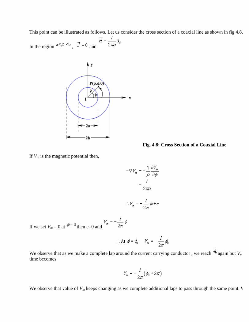
This point can be illustrated as follows. Let us consider the cross section of a coaxial line as shown in fig 4.8.

In the region , and

Fig. 4.8: Cross Section of a Coaxial Line

If Vm is the magnetic potential then,

If we set Vm = 0 at then c=0 and

We observe that as we make a complete lap around the current carrying conductor , we reach again but Vm this

time becomes

We observe that value of Vm keeps changing as we complete additional laps to pass through the same point. We

introduced Vm analogous to electostatic potential V. But for static electric fields, and ,

whereas for steady magnetic field wherever but even if along the path of

integration.

We now introduce the vector magnetic potential which can be used in regions where current density may be zero or

nonzero and the same can be easily extended to time varying cases. The use of vector magnetic potential provides

elegant ways of solving EM field problems.

Since and we have the vector identity that for any vector , , we can write .

Here, the vector field is called the vector magnetic potential. Its SI unit is Wb/m. Thus if can find of a given

current distribution, can be found from through a curl operation.

We have introduced the vector function and related its curl to . A vector function is defined fully in terms of

its curl as well as divergence. The choice of is made as follows.

...........................................(4.24)

By using vector identity, .................................................(4.25)

.........................................(4.26)

Great deal of simplification can be achieved if we choose .

Putting , we get which is vector poisson equation.

In Cartesian coordinates, the above equation can be written in terms of the components as

......................................(4.27a)

......................................(4.27b)

......................................(4.27c)

The form of all the above equation is same as that of

..........................................(4.28)

for which the solution is

..................(4.29)

In case of time varying fields we shall see that , which is known as Lorentz condition, V being the

electric potential. Here we are dealing with static magnetic field, so .

By comparison, we can write the solution for Ax as

...................................(4.30)

Computing similar solutions for other two components of the vector potential, the vector potential can be written as

.......................................(4.31)

This equation enables us to find the vector potential at a given point because of a volume current density .

Similarly for line or surface current density we can write

...................................................(4.32)

respectively. ..............................(4.33)

The magnetic flux through a given area S is given by

.............................................(4.34)

Substituting

.........................................(4.35)

Vector potential thus have the physical significance that its integral around any closed path is equal to the magnetic

flux passing through that path.

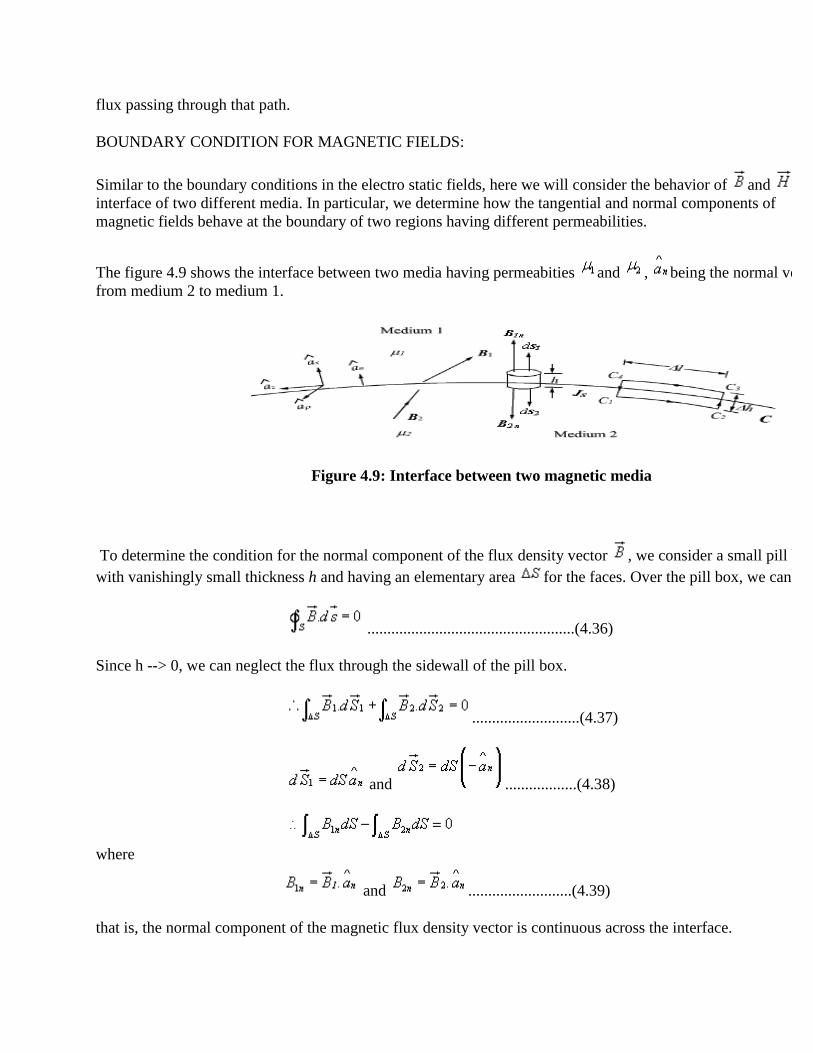
BOUNDARY CONDITION FOR MAGNETIC FIELDS:

Similar to the boundary conditions in the electro static fields, here we will consider the behavior of and at the

interface of two different media. In particular, we determine how the tangential and normal components of

magnetic fields behave at the boundary of two regions having different permeabilities.

The figure 4.9 shows the interface between two media having permeabities and , being the normal vector

from medium 2 to medium 1.

Figure 4.9: Interface between two magnetic media

To determine the condition for the normal component of the flux density vector , we consider a small pill box P

with vanishingly small thickness h and having an elementary area for the faces. Over the pill box, we can write

....................................................(4.36)

Since h --> 0, we can neglect the flux through the sidewall of the pill box.

...........................(4.37)

and ..................(4.38)

where

and ..........................(4.39)

that is, the normal component of the magnetic flux density vector is continuous across the interface.

In vector form,

...........................(4.41)

To determine the condition for the tangential component for the magnetic field, we consider a closed path C as

shown in figure 4.8. By applying Ampere's law we can write

....................................(4.42)

since is small, we can write

or, ...................................(4.40)

That is, the normal component of the magnetic flux density vector is continuous across the interface.

In vector form,

...........................(4.41)

To determine the condition for the tangential component for the magnetic field, we consider a closed path C as

shown in figure 4.8. By applying Ampere's law we can write

....................................(4.42)

...................................(4.45)

Therefore,

...................................(4.46)

if Js = 0, the tangential magnetic field is also continuous. If one of the medium is a perfect conductor Js exists on

the surface of the perfect conductor.

In vector form we can write,

...................................(4.45) Therefore,

...................................(4.46)

UNIT II STATIC MAGNETIC FIELD PART- A (2 MARKS) 1. State coulombs law. 2. State Gauss law for electric fields 3. Define electric flux & electric flux density 4. Define electric field intensity 5. Name few applications of Gauss law in electrostatics 6. Define potential difference. 7. Define potential. 8. Give the relation between electric field intensity and electric flux density.

9. Give the relationship between potential gradient and electric field. 10. Define current density. 11. Write down the expression for capacitance between two parallel plates. 12. State point form of ohms law. 13. Define dielectric strength.

PART- B 1. State and proof gauss law .and explain applications of gauss law. (16) 2. Drive an expression for the electric field due to a straight and infinite Uniformly charged wire of length ‘L’ meters and with a charge density of +_ c/m at a point P which lies along the perpendicular bisector of wire. (16) 3 . (a) Explain poissons and lapace’s equations. (8) .(b) A uniform line charge _L =25Nc/m lies on the x=3m and y=4m in free space . find the electric field intensity at a point (2,3,15)m. (8) 4. A circular disc of radius‘a’ m is charged uniformly with a charge density of c/ m2.find the electric field at a point ‘h’ m from the disc along its axis. (16) 5 (a).Define the potential difference and absolute potential. Give the relation between potential and field intensity. (8) (b) A circular disc of 10 cm radius is charged uniformly with a total charge 10-10c.find the electric field at a point 30 cm away from the disc along the axis. (8) 7. Derive the boundary conditions of the normal and tangential components of electric field at the inter face of two media with different dielectrics. (16) 8. (a) Derive an expression for the capacitance of a parallel plate capacitor having two dielectric media. (8) (b) Derive an expression for the capacitance of two wire transmission line. (8) 9. . Drive an expression for energy stored and energy density in electrostatic field. (16) 10 (a) Derive an expression for capacitance of concentric spheres. (8) (b) Derive an expression for capacitance of co-axial cable. (8) 11 (a) Explain and derive the polarization of a dielectric materials. (8) (b) List out the properties of dielectric materials. (8) 12.The capacitance of the conductor formed by the two parallel metal sheets, each 100cm2,in area separated by a dielectric 2mm thick is , 2x10-10 micro farad .a potential of 20KV is applied to it .find (i) Electric flux (ii) Potential gradient in kV/m

UNIT III ELECTRIC AND MAGNETIC FIELDS IN MATERIALS

Poisson‟s and laplace‟s equation – Electric polarization – Nature of dielectric materials –

Definition of capacitance – Capacitance of various geometries using laplace‟s equation –

Electrostatic energy and energy density – Boundary conditions for electric fields –

Electric current – Current density – Point form of ohm‟s law – Continuity equation for

current – Definition of inductance – Inductance of loops and solenoids – Definition of

mutual inductance – Simple examples – Energy density in magnetic fields – Nature of

magnetic materials – Magnetization and permeability – Magnetic boundary conditions.

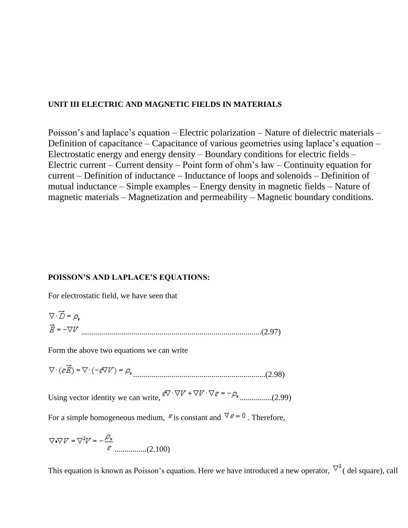
POISSON’S AND LAPLACE’S EQUATIONS:

For electrostatic field, we have seen that

..........................................................................................(2.97)

Form the above two equations we can write

..................................................................(2.98)

Using vector identity we can write, ................(2.99)

For a simple homogeneous medium, is constant and . Therefore,

................(2.100)

This equation is known as Poisson‟s equation. Here we have introduced a new operator, ( del square), called the

Laplacian operator. In Cartesian coordinates,

...............(2.101)

Therefore, in Cartesian coordinates, Poisson equation can be written as:

...............(2.102)

In cylindrical coordinates,

...............(2.103)

n spherical polar coordinate system,

...............(2.104)

At points in simple media, where no free charge is present, Poisson‟s equation reduces to

...................................(2.105)

which is known as Laplace‟s equation.

Laplace‟s and Poisson‟s equation are very useful for solving many practical electrostatic field problems where only

the electrostatic conditions (potential and charge) at some boundaries are known and solution of electric field and

potential is to be found throughout the volume. We shall consider such applications in the section where we deal

with boundary value problems.

CAPACITANCE AND CAPACITORS

We have already stated that a conductor in an electrostatic field is an Equipotential body and any charge given to

such conductor will distribute themselves in such a manner that electric field inside the conductor vanishes. If an

additional amount of charge is supplied to an isolated conductor at a given potential, this additional charge will

increase the surface charge density . Since the potential of the conductor is given by , the

potential of the conductor will also increase maintaining the ratio same. Thus we can write where the

constant of proportionality C is called the capacitance of the isolated conductor. SI unit of capacitance is Coulomb/

Volt also called Farad denoted by F. It can It can be seen that if V=1, C = Q. Thus capacity of an isolated conductor

can also be defined as the amount of charge in Coulomb required to raise the potential of the conductor by 1 Volt.

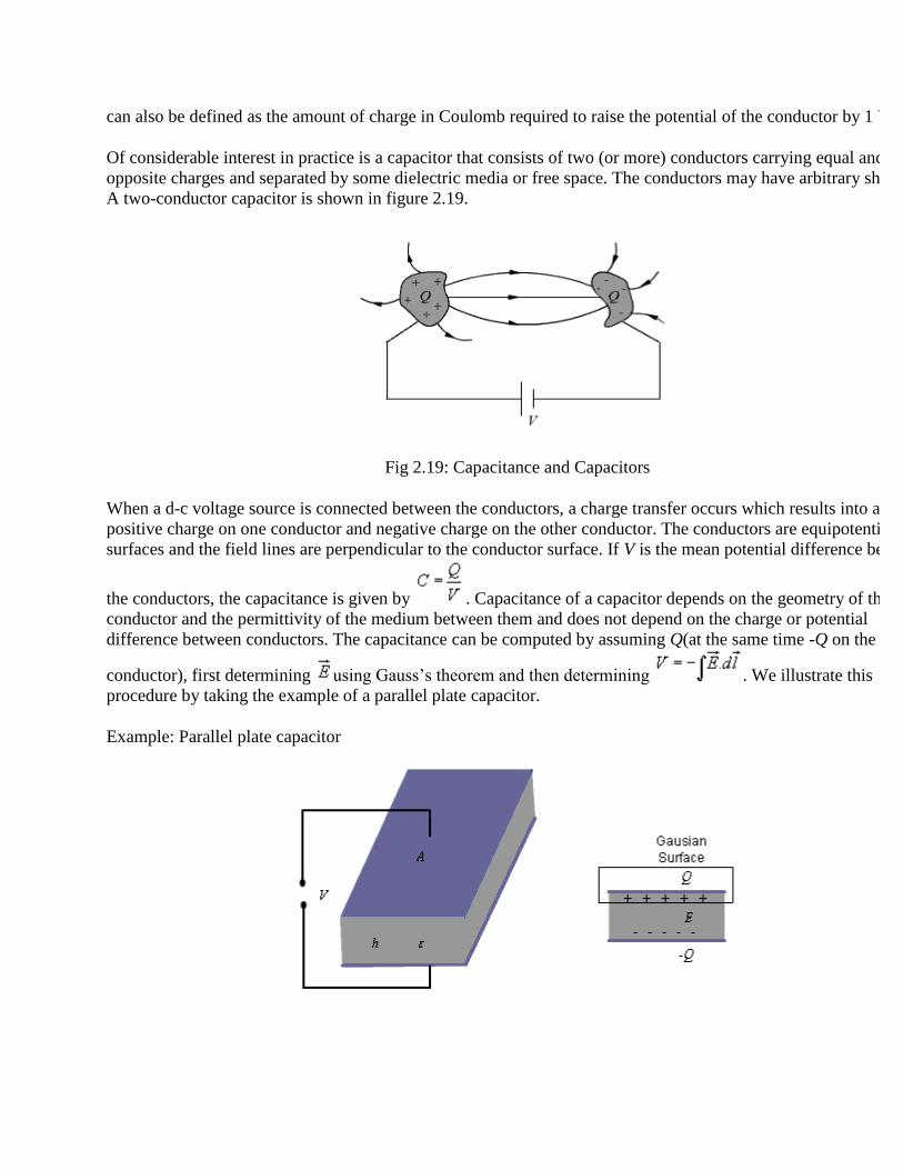
Of considerable interest in practice is a capacitor that consists of two (or more) conductors carrying equal and

opposite charges and separated by some dielectric media or free space. The conductors may have arbitrary shapes.

A two-conductor capacitor is shown in figure 2.19.

Fig 2.19: Capacitance and Capacitors

When a d-c voltage source is connected between the conductors, a charge transfer occurs which results into a

positive charge on one conductor and negative charge on the other conductor. The conductors are equipotential

surfaces and the field lines are perpendicular to the conductor surface. If V is the mean potential difference between

the conductors, the capacitance is given by . Capacitance of a capacitor depends on the geometry of the

conductor and the permittivity of the medium between them and does not depend on the charge or potential

difference between conductors. The capacitance can be computed by assuming Q(at the same time -Q on the other

conductor), first determining using Gauss‟s theorem and then determining . We illustrate this

procedure by taking the example of a parallel plate capacitor.

Example: Parallel plate capacitor

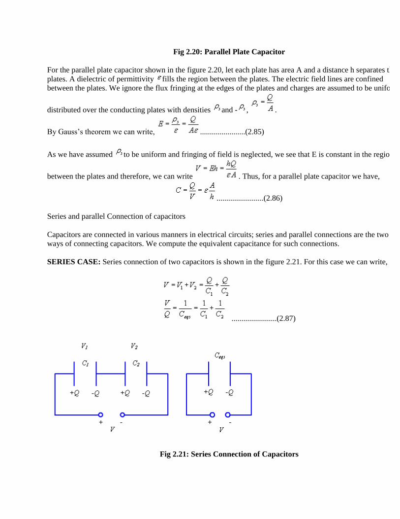
Fig 2.20: Parallel Plate Capacitor

For the parallel plate capacitor shown in the figure 2.20, let each plate has area A and a distance h separates the

plates. A dielectric of permittivity fills the region between the plates. The electric field lines are confined

between the plates. We ignore the flux fringing at the edges of the plates and charges are assumed to be uniformly

distributed over the conducting plates with densities and - , .

By Gauss‟s theorem we can write, .......................(2.85)

As we have assumed to be uniform and fringing of field is neglected, we see that E is constant in the region

between the plates and therefore, we can write . Thus, for a parallel plate capacitor we have,

........................(2.86)

Series and parallel Connection of capacitors

Capacitors are connected in various manners in electrical circuits; series and parallel connections are the two basic

ways of connecting capacitors. We compute the equivalent capacitance for such connections.

SERIES CASE: Series connection of two capacitors is shown in the figure 2.21. For this case we can write,

.......................(2.87)

Fig 2.21: Series Connection of Capacitors

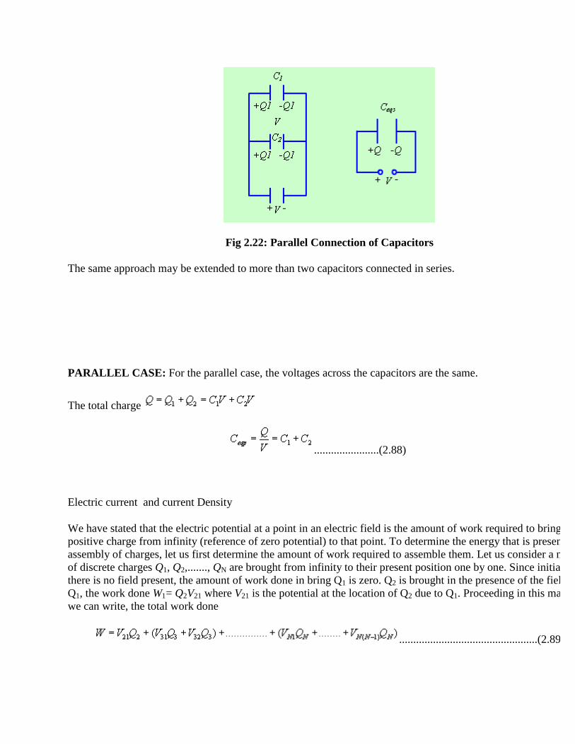
Fig 2.22: Parallel Connection of Capacitors

The same approach may be extended to more than two capacitors connected in series.

PARALLEL CASE: For the parallel case, the voltages across the capacitors are the same.

The total charge

.......................(2.88)

Electric current and current Density

We have stated that the electric potential at a point in an electric field is the amount of work required to bring a unit

positive charge from infinity (reference of zero potential) to that point. To determine the energy that is present in an

assembly of charges, let us first determine the amount of work required to assemble them. Let us consider a number

of discrete charges Q1, Q2,......., QN are brought from infinity to their present position one by one. Since initially

there is no field present, the amount of work done in bring Q1 is zero. Q2 is brought in the presence of the field of

Q1, the work done W1= Q2V21 where V21 is the potential at the location of Q2 due to Q1. Proceeding in this manner,

we can write, the total work done

.................................................(2.89)

Had the charges been brought in the reverse order,

.................(2.90)

Therefore,

................(2.91)

Here VIJ represent voltage at the Ith

charge location due to Jth

charge. Therefore,

Or, ................(2.92)

If instead of discrete charges, we now have a distribution of charges over a volume v then we can write,

................(2.93)

where is the volume charge density and V represents the potential function.

Since, , we can write

.......................................(2.94)

Using the vector identity,

, we can write

................(2.95)

In the expression , for point charges, since V varies as and D varies as , the term V varies as

while the area varies as r2. Hence the integral term varies at least as and the as surface becomes large (i.e.

) the integral term tends to zero.

Thus the equation for W reduces to

................(2.96)

, is called the energy density in the electrostatic field.

CURRENT DENSITY AND OHM'S LAW:

In our earlier discussion we have mentioned that, conductors have free electrons that move randomly under thermal

agitation. In the absence of an external electric field, the average thermal velocity on a microscopic scale is zero

and so is the net current in the conductor. Under the influence of an applied field, additional velocity is

superimposed on the random velocities. While the external field accelerates the electron in a direction opposite to

it, the collision with atomic lattice however provide the frictional mechanism by which the electrons lose some of

the momentum gained between the collisions. As a result, the electrons move with some average drift velocity .

This drift velocity can be related to the applied electric field by the relationship

......................(3.1)

where is the average time between the collisions.

The quantity i.e., the the drift velocity per unit applied field is called the mobility of electrons and denoted by

.

Thus , e is the magnitude of the electronic charge and , as the electron drifts opposite to the

applied field.

t us consider a conductor under the influence of an external electric field. If represents the number of electrons

per unit volume, then the charge crossing an area that is normal to the direction of the drift velocity is given

by:

........................................(3.2)

This flow of charge constitutes a current across , which is given by,

................(3.3)

The conduction current density can therefore be expressed as

.................................(3.4)

where is called the conductivity. In vector form, we can write,

..........................................................(3.5)

The above equation is the alternate way of expressing Ohm's law and this relationship is valid at a point.

For semiconductor material, current flow is both due to electrons and holes (however in practice, it the electron

which moves), we can write

......................(3.6)

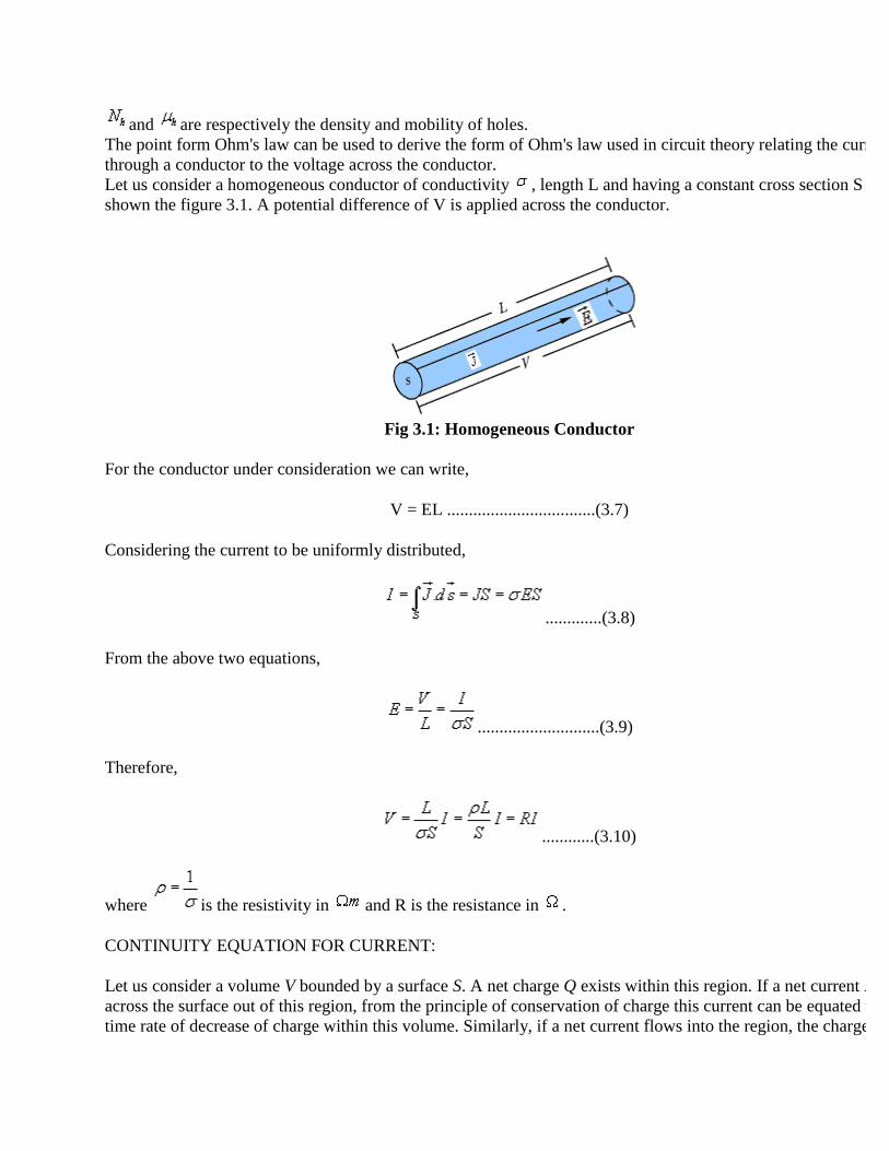
and are respectively the density and mobility of holes.

The point form Ohm's law can be used to derive the form of Ohm's law used in circuit theory relating the current

through a conductor to the voltage across the conductor.

Let us consider a homogeneous conductor of conductivity , length L and having a constant cross section S as

shown the figure 3.1. A potential difference of V is applied across the conductor.

Fig 3.1: Homogeneous Conductor

For the conductor under consideration we can write,

V = EL ..................................(3.7)

Considering the current to be uniformly distributed,

.............(3.8)

From the above two equations,

............................(3.9)

Therefore,

............(3.10)

where is the resistivity in and R is the resistance in .

CONTINUITY EQUATION FOR CURRENT:

Let us consider a volume V bounded by a surface S. A net charge Q exists within this region. If a net current I flows

across the surface out of this region, from the principle of conservation of charge this current can be equated to the

time rate of decrease of charge within this volume. Similarly, if a net current flows into the region, the charge in the

volume must increase at a rate equal to the current. Thus we can write,

.....................................(3.17)

or, ......................(3.18)

Applying divergence theorem we can write,

.....................(3.19)

It may be noted that, since in general may be a function of space and time, partial derivatives are used. Further,

the equation holds regardless of the choice of volume V , the integrands must be equal.

Therefore we can write,

................(3.20)

The equation (3.20) is called the continuity equation, which relates the divergence of current density vector to the

rate of change of charge density at a point.

For steady current flowing in a region, we have

......................(3.21)

Considering a region bounded by a closed surface,

..................(3.22)

which can be written as,

......................(3.23)

when we consider the close surface essentially encloses a junction of an electrical circuit.

The above equation is the Kirchhoff‟s current law of circuit theory, which states that algebraic sum of all the

currents flowing out of a junction in an electric circuit, is zero.

INDUCTANCE AND INDUCTOR:

Resistance, capacitance and inductance are the three familiar parameters from circuit theory. We have already

discussed about the parameters resistance and capacitance in the earlier chapters. In this section, we discuss about

the parameter inductance. Before we start our discussion, let us first introduce the concept of flux linkage. If in a

coil with N closely wound turns around where a current I produces a flux and this flux links or encircles each of

the N turns, the flux linkage is defined as . In a linear medium, where the flux is proportional to the

current, we define the self inductance L as the ratio of the total flux linkage to the current which they link.

i.e., ...................................(4.47)

To further illustrate the concept of inductance, let us consider two closed loops C1 and C2 as shown in the figure

4.10, S1 and S2 are respectively the areas of C1 and C2 .

Fig 4.10

If a current I1 flows in C1 , the magnetic flux B1 will be created part of which will be linked to C2 as shown in

Figure 4.10.

...................................(4.48)

In a linear medium, is proportional to I 1. Therefore, we can write

...................................(4.49)

where L12 is the mutual inductance. For a more general case, if C2 has N2 turns then

...................................(4.50)

and

or ...................................(4.51)

i.e., the mutual inductance can be defined as the ratio of the total flux linkage of the second circuit to the current

flowing in the first circuit.

As we have already stated, the magnetic flux produced in C1 gets linked to itself and if C1 has N1 turns then

, where is the flux linkage per turn.

Therefore, self inductance

= ...................................(4.52)

As some of the flux produced by I1 links only to C1 & not C2.

...................................(4.53)

Further in general, in a linear medium, and

Fig 4.11: A long current carrying solenoid

The magnetic flux density inside such a long solenoid can be calculated as

..................................(4.54)

where the magnetic field is along the axis of the solenoid.

ENERGY DENSITY IN MAGNETIC FIELD:

So far we have discussed the inductance in static forms. In earlier chapter we discussed the fact that work is

required to be expended to assemble a group of charges and this work is stated as electric energy. In the same

manner energy needs to be expended in sending currents through coils and it is stored as magnetic energy. Let us

consider a scenario where we consider a coil in which the current is increased from 0 to a value I. As mentioned

earlier, the self inductance of a coil in general can be written as

..................................(4.70a)

or ..................................(4.70b)

If we consider a time varying scenario,

..................................(4.71)

We will later see that is an induced voltage.

. .................................(4.72)

& (Joule)...................................(4.73)

which is the energy stored in the magnetic circuit.

We can also express the energy stored in the coil in term of field quantities.

For linear magnetic circuit

...................................(4.74)

Now, ...................................(4.75)

where A is the area of cross section of the coil. If l is the length of the coil

...................................(4.76)

Al is the volume of the coil. Therefore the magnetic energy density i.e., magnetic energy/unit volume is given by

...................................(4.77)

In vector form

J/mt3 ...................................(4.78)

is the energy density in the magnetic field.

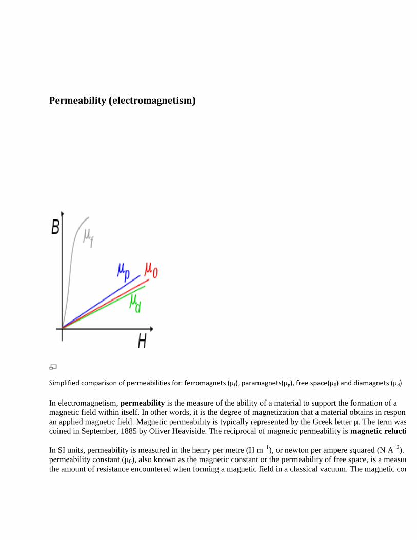
Permeability (electromagnetism)

Simplified comparison of permeabilities for: ferromagnets (μf), paramagnets(μp), free space(μ0) and diamagnets (μd)

In electromagnetism, permeability is the measure of the ability of a material to support the formation of a

magnetic field within itself. In other words, it is the degree of magnetization that a material obtains in response to

an applied magnetic field. Magnetic permeability is typically represented by the Greek letter μ. The term was

coined in September, 1885 by Oliver Heaviside. The reciprocal of magnetic permeability is magnetic reluctivity.

In SI units, permeability is measured in the henry per metre (H m−1

), or newton per ampere squared (N A−2

). The

permeability constant (μ0), also known as the magnetic constant or the permeability of free space, is a measure of

the amount of resistance encountered when forming a magnetic field in a classical vacuum. The magnetic constant

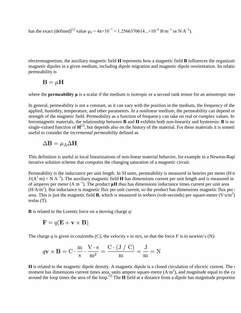
has the exact (defined)[1]

value µ0 = 4π×10−7

≈ 1.2566370614...×10−6

H·m−1

or N·A−2

).

electromagnetism, the auxiliary magnetic field H represents how a magnetic field B influences the organization of

magnetic dipoles in a given medium, including dipole migration and magnetic dipole reorientation. Its relation to

permeability is

where the permeability μ is a scalar if the medium is isotropic or a second rank tensor for an anisotropic medium.

In general, permeability is not a constant, as it can vary with the position in the medium, the frequency of the field

applied, humidity, temperature, and other parameters. In a nonlinear medium, the permeability can depend on the

strength of the magnetic field. Permeability as a function of frequency can take on real or complex values. In

ferromagnetic materials, the relationship between B and H exhibits both non-linearity and hysteresis: B is not a

single-valued function of H[2]

, but depends also on the history of the material. For these materials it is sometimes

useful to consider the incremental permeability defined as

.

This definition is useful in local linearizations of non-linear material behavior, for example in a Newton-Raphson

iterative solution scheme that computes the changing saturation of a magnetic circuit.

Permeability is the inductance per unit length. In SI units, permeability is measured in henries per meter (H·m−1

=

J/(A2·m) = N A

−2). The auxiliary magnetic field H has dimensions current per unit length and is measured in units

of amperes per meter (A m−1

). The product μH thus has dimensions inductance times current per unit area

(H·A/m2). But inductance is magnetic flux per unit current, so the product has dimensions magnetic flux per unit

area. This is just the magnetic field B, which is measured in webers (volt-seconds) per square-meter (V·s/m2), or

teslas (T).

B is related to the Lorentz force on a moving charge q:

.

The charge q is given in coulombs (C), the velocity v in m/s, so that the force F is in newton‟s (N):

H is related to the magnetic dipole density. A magnetic dipole is a closed circulation of electric current. The dipole

moment has dimensions current times area, units ampere square-metre (A·m2), and magnitude equal to the current

around the loop times the area of the loop.[3]

The H field at a distance from a dipole has magnitude proportional to

the dipole moment divided by distance cubed[4]

, which has dimensions current per unit length. Relative

permeability

Relative permeability, sometimes denoted by the symbol μr, is the ratio of the permeability of a specific medium to

the permeability of free space given by the magnetic constant :

.

In terms of relative permeability, the magnetic susceptibility is:

χm = μr − 1.

χm, a dimensionless quantity, is sometimes called volumetric or bulk susceptibility, to distinguish it from χ

UNIT III ELECTRIC AND MAGNETIC FIELDS IN MATERIALS

PART- A (2 MARKS) 1. State Biot –savarts law. 2. State Ampere circuital law 3. Write the relation between magnetic flux density and field intensity 4. Write the relation between relative permeability and suspectibility 5. Define magnetic flux density 6. Write down the magnetic boundary conditions. 7. Give the force on a current element. 8. Define magnetic moment. 9. State Gauss law for magnetic field. 10. What is magnetic susceptibility 11. Define magnetic dipole. 12. Give torque on closed circuits 13. Define magnetization. 14. List the types of magnetic materials

PART- B 1. Derive the expressions for magnetic field intensity due to finite and infinite line (16) 2. Derive the expressions for magnetic flux intensity due to solenoid of the coil. (16) 3. Derive the expressions for magnetic field intensity due to toroidal coil and circular coil. (16) 4. Derive an expressions for energy stored and energy density in magnetic field. (16) 5. (a) Derive an expressions for self inductance of two wire transmission line. (8) (b) Derive an expressions for force between two current carrying conductors. (8)

6 (a) Derive the expression for torque developed in a rectangular closed circuit carrying current I a uniform field. (8) (b) An iron ring with a cross sectional area of 3cm square and mean circumference of 15 cm is wound with 250 turns wire carrying a current of 0.3A.The relative permeability of ring is 1500.calculate the flux established in the ring. (8 7. Explain Magnetic materials and scalar and vector magnetic potentials. (16 ) 8. Derive the expressions for boundary conditions in magnetic fields. (16) 9. A solenoid 25cm long ,1cm mean diameter of the coil turns a uniformly Distributed windings of 2000 turns .the solenoid is placed in uniform field of 2tesla flux density. a current of 5a is passed through the winding. Determine the (i) Maximum torque on the solenoid& (ii) Maximum force on the solenoid (iii) Compute the magnetic moment on the solenoid. (16) 10 (a).Derive the expression for co-efficient of coupling in terms of mutual and self inductance (8) (b) Calculate the inductance of a solenoid of 200 turns wound tightly on a cylindrical tube of 6cm diameter .The length of the tube is 60cm and the solenoid is air. (8) 11 (a). Define and explain biot –savart law (8) (b) Find H at the centre of an equivalent triangular loop of side 4m carrying current of 5A. (8)

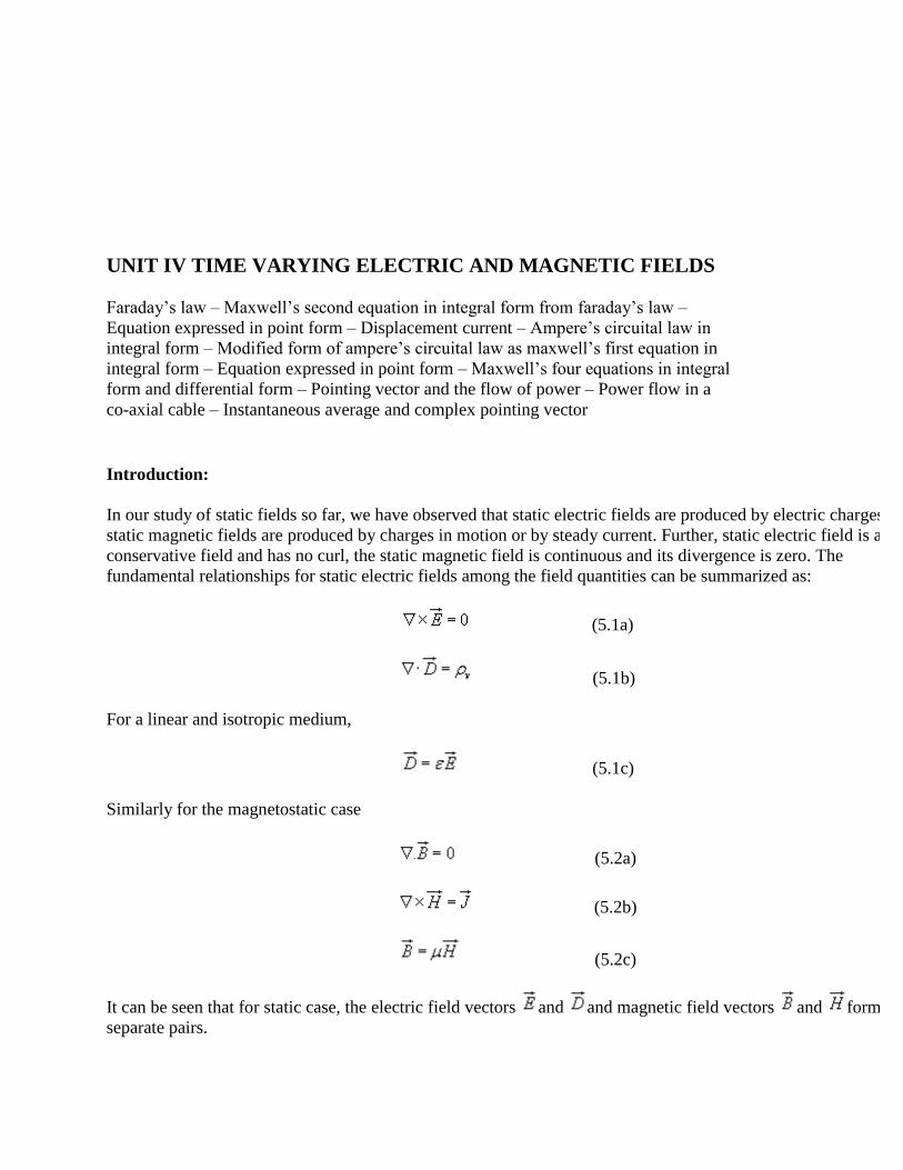
UNIT IV TIME VARYING ELECTRIC AND MAGNETIC FIELDS

Faraday‟s law – Maxwell‟s second equation in integral form from faraday‟s law –

Equation expressed in point form – Displacement current – Ampere‟s circuital law in

integral form – Modified form of ampere‟s circuital law as maxwell‟s first equation in

integral form – Equation expressed in point form – Maxwell‟s four equations in integral

form and differential form – Pointing vector and the flow of power – Power flow in a

co-axial cable – Instantaneous average and complex pointing vector

Introduction:

In our study of static fields so far, we have observed that static electric fields are produced by electric charges,

static magnetic fields are produced by charges in motion or by steady current. Further, static electric field is a

conservative field and has no curl, the static magnetic field is continuous and its divergence is zero. The

fundamental relationships for static electric fields among the field quantities can be summarized as:

(5.1a)

(5.1b)

For a linear and isotropic medium,

(5.1c)

Similarly for the magnetostatic case

(5.2a)

(5.2b)

(5.2c)

It can be seen that for static case, the electric field vectors and and magnetic field vectors and form

separate pairs.

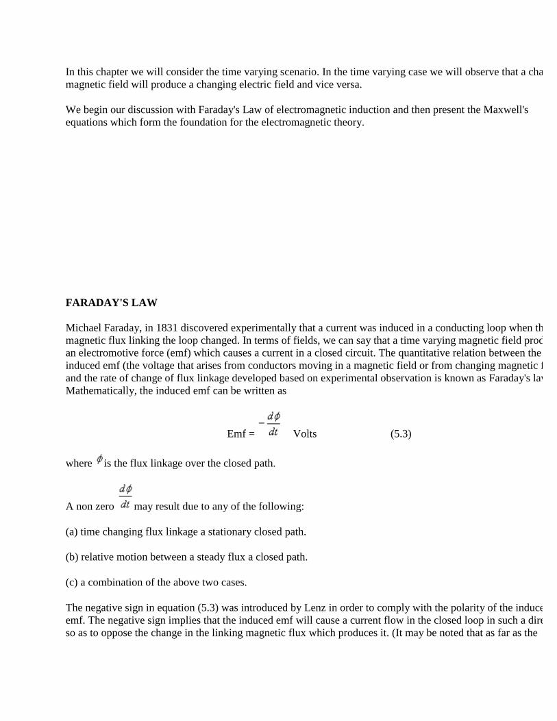
In this chapter we will consider the time varying scenario. In the time varying case we will observe that a changing

magnetic field will produce a changing electric field and vice versa.

We begin our discussion with Faraday's Law of electromagnetic induction and then present the Maxwell's

equations which form the foundation for the electromagnetic theory.

FARADAY'S LAW

Michael Faraday, in 1831 discovered experimentally that a current was induced in a conducting loop when the

magnetic flux linking the loop changed. In terms of fields, we can say that a time varying magnetic field produces

an electromotive force (emf) which causes a current in a closed circuit. The quantitative relation between the

induced emf (the voltage that arises from conductors moving in a magnetic field or from changing magnetic fields)

and the rate of change of flux linkage developed based on experimental observation is known as Faraday's law.

Mathematically, the induced emf can be written as

Emf = Volts (5.3)

where is the flux linkage over the closed path.

A non zero may result due to any of the following:

(a) time changing flux linkage a stationary closed path.

(b) relative motion between a steady flux a closed path.

(c) a combination of the above two cases.

The negative sign in equation (5.3) was introduced by Lenz in order to comply with the polarity of the induced

emf. The negative sign implies that the induced emf will cause a current flow in the closed loop in such a direction

so as to oppose the change in the linking magnetic flux which produces it. (It may be noted that as far as the

induced emf is concerned, the closed path forming a loop does not necessarily have to be conductive).

If the closed path is in the form of N tightly wound turns of a coil, the change in the magnetic flux linking the coil

induces an emf in each turn of the coil and total emf is the sum of the induced emfs of the individual turns, i.e.,

Emf = Volts (5.4)

By defining the total flux linkage as

(5.5)

The emf can be written as

Emf = (5.6)

Continuing with equation (5.3), over a closed contour 'C' we can write

Emf = (5.7)

where is the induced electric field on the conductor to sustain the current.

urther, total flux enclosed by the contour 'C ' is given by

(5.8)

Where S is the surface for which 'C' is the contour.

From (5.7) and using (5.8) in (5.3) we can write

(5.9)

By applying stokes theorem

(5.10)

Therefore, we can write

(5.11)

FARADAY'S LAW IN THE POINT FORM :

We have said that non zero can be produced in a several ways. One particular case is when a time varying flux

linking a stationary closed path induces an emf. The emf induced in a stationary closed path by a time varying

magnetic field is called a transformer emf .

MOTIONAL EMF:

Let us consider a conductor moving in a steady magnetic field as shown in the fig 5.2.

Fig 5.2

If a charge Q moves in a magnetic field , it experiences a force

(5.18)

This force will cause the electrons in the conductor to drift towards one end and leave the other end positively

charged, thus creating a field and charge separation continuous until electric and magnetic forces balance and an

equilibrium is reached very quickly, the net force on the moving conductor is zero.

can be interpreted as an induced electric field which is called the motional electric field

(5.19)

If the moving conductor is a part of the closed circuit C, the generated emf around the circuit is . This

emf is called the motional emf.

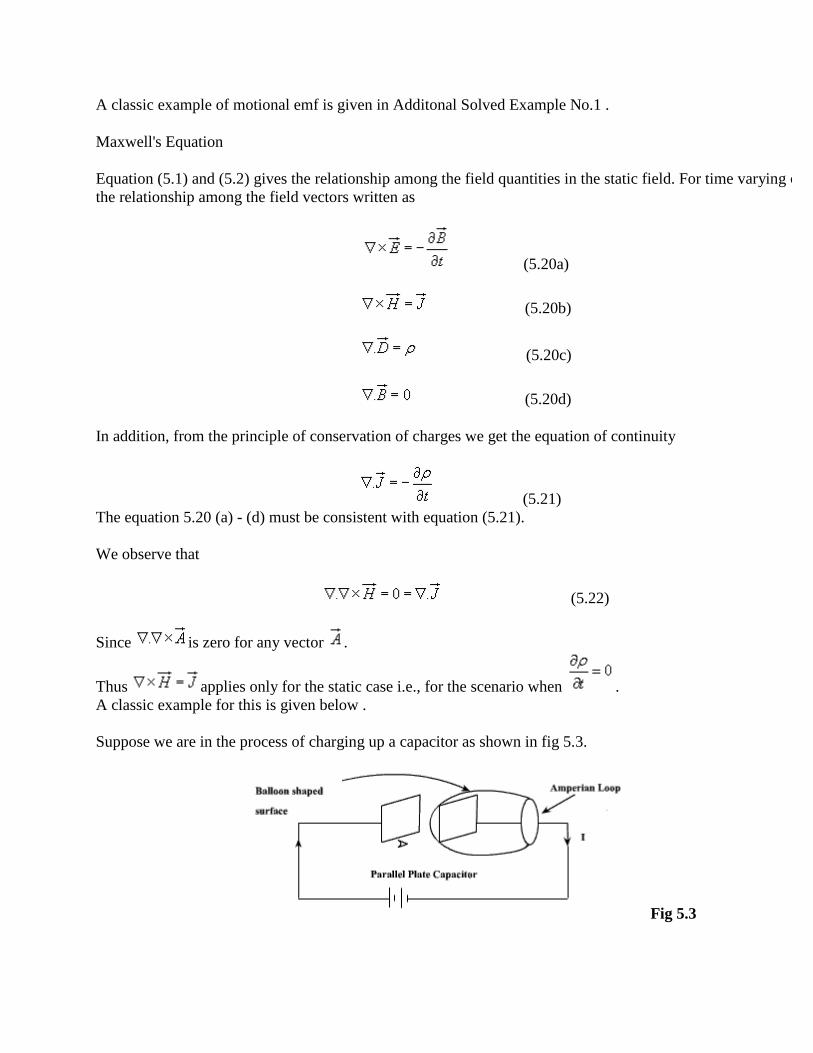
A classic example of motional emf is given in Additonal Solved Example No.1 .

Maxwell's Equation

Equation (5.1) and (5.2) gives the relationship among the field quantities in the static field. For time varying case,

the relationship among the field vectors written as

(5.20a)

(5.20b)

(5.20c)

(5.20d)

In addition, from the principle of conservation of charges we get the equation of continuity

(5.21)

The equation 5.20 (a) - (d) must be consistent with equation (5.21).

We observe that

(5.22)

Since is zero for any vector .

Thus applies only for the static case i.e., for the scenario when .

A classic example for this is given below .

Suppose we are in the process of charging up a capacitor as shown in fig 5.3.

Fig 5.3

Let us apply the Ampere's Law for the Amperian loop shown in fig 5.3. Ienc = I is the total current passing through

the loop. But if we draw a baloon shaped surface as in fig 5.3, no current passes through this surface and hence Ienc

= 0. But for non steady currents such as this one, the concept of current enclosed by a loop is ill-defined since it

depends on what surface you use. In fact Ampere's Law should also hold true for time varying case as well, then

comes the idea of displacement current which will be introduced in the next few slides.

We can write for time varying case,

(5.23)

(5.24)

The equation (5.24) is valid for static as well as for time varying case.

Equation (5.24) indicates that a time varying electric field will give rise to a magnetic field even in the absence of

. The term has a dimension of current densities and is called the displacement current density.

Introduction of in equation is one of the major contributions of Jame's Clerk Maxwell. The modified set

of equations

(5.25a)

(5.25b)

(5.25c)

(5.25d)

is known as the Maxwell's equation and this set of equations apply in the time varying scenario, static fields are

being a particular case .

In the integral form

(5.26a)

(5.26b)

(5.26c)

(5.26d)

The modification of Ampere's law by Maxwell has led to the development of a unified electromagnetic field

theory. By introducing the displacement current term, Maxwell could predict the propagation of EM waves.

Existence of EM waves was later demonstrated by Hertz experimentally which led to the new era of radio

communication.

BOUNDARY CONDITIONS FOR ELECTROMAGNETIC FIELDS

The differential forms of Maxwell's equations are used to solve for the field vectors provided the field quantities

are single valued, bounded and continuous. At the media boundaries, the field vectors are discontinuous and their

behaviors across the boundaries are governed by boundary conditions. The integral equations(eqn 5.26) are

assumed to hold for regions containing discontinuous media.Boundary conditions can be derived by applying the

Maxwell's equations in the integral form to small regions at the interface of the two media. The procedure is similar

to those used for obtaining boundary conditions for static electric fields (chapter 2) and static magnetic fields

(chapter 4). The boundary conditions are summarized as follows

With reference to fig 5.3

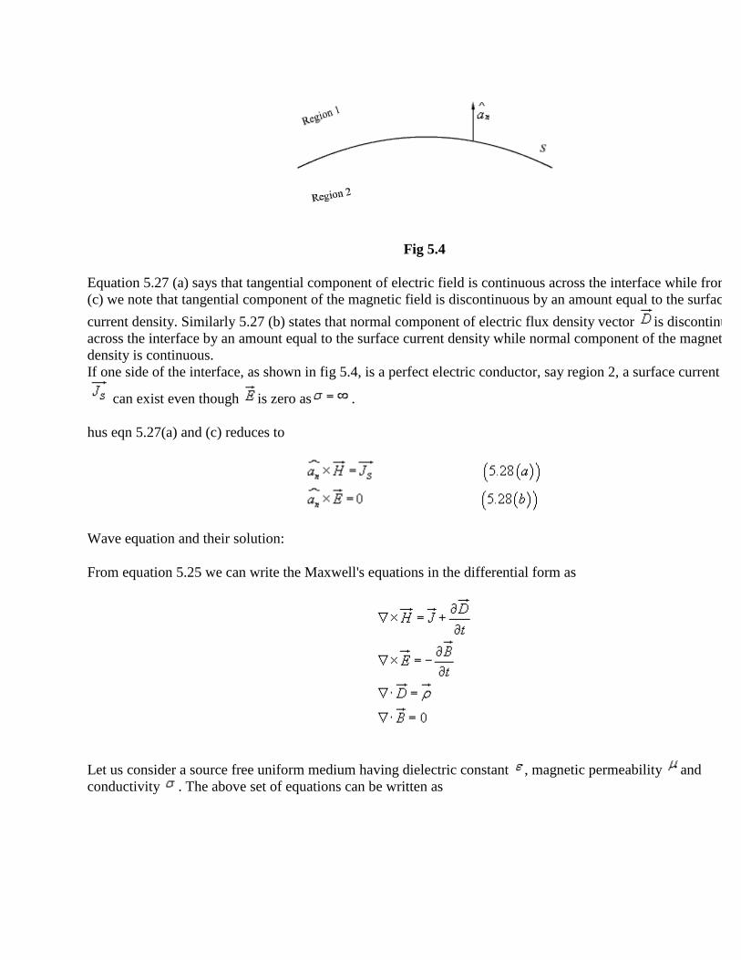
Fig 5.4

Equation 5.27 (a) says that tangential component of electric field is continuous across the interface while from 5.27

(c) we note that tangential component of the magnetic field is discontinuous by an amount equal to the surface

current density. Similarly 5.27 (b) states that normal component of electric flux density vector is discontinuous

across the interface by an amount equal to the surface current density while normal component of the magnetic flux

density is continuous.

If one side of the interface, as shown in fig 5.4, is a perfect electric conductor, say region 2, a surface current

can exist even though is zero as .

hus eqn 5.27(a) and (c) reduces to

Wave equation and their solution:

From equation 5.25 we can write the Maxwell's equations in the differential form as

Let us consider a source free uniform medium having dielectric constant , magnetic permeability and

conductivity . The above set of equations can be written as

Using the vector identity ,

We can write from 5.29(b)

or

Substituting from 5.29(a)

But in source free medium (eqn 5.29(c))

(5.30)

In the same manner for equation eqn 5.29(a)

Since from eqn 5.29(d), we can write

(5.31)

These two equations

are known as wave equations.

It may be noted that the field components are functions of both space and time. For example, if we consider a

Cartesian co ordinate system, essentially represents and . For simplicity, we

consider propagation in free space , i.e. , and . The wave eqn in equations 5.30 and 5.31 reduces

to

Further simplifications can be made if we consider in Cartesian co ordinate system a special case where

are considered to be independent in two dimensions, say are assumed to be independent of y and

z. Such waves are called plane waves.

From eqn (5.32 (a)) we can write

The vector wave equation is equivalent to the three scalar equations

Since we have ,

As we have assumed that the field components are independent of y and z eqn (5.34) reduces to

(5.35)

i.e. there is no variation of Ex in the x direction.

Further, from 5.33(a), we find that implies which requires any three of the conditions to be

satisfied: (i) Ex=0, (ii)Ex = constant, (iii)Ex increasing uniformly with time.

A field component satisfying either of the last two conditions (i.e (ii) and (iii))is not a part of a plane wave motion

and hence Ex is taken to be equal to zero. Therefore, a uniform plane wave propagating in x direction does not have

a field component (E or H) acting along x.

Without loss of generality let us now consider a plane wave having Ey component only (Identical results can be

obtained for Ez component) .

The equation involving such wave propagation is given by

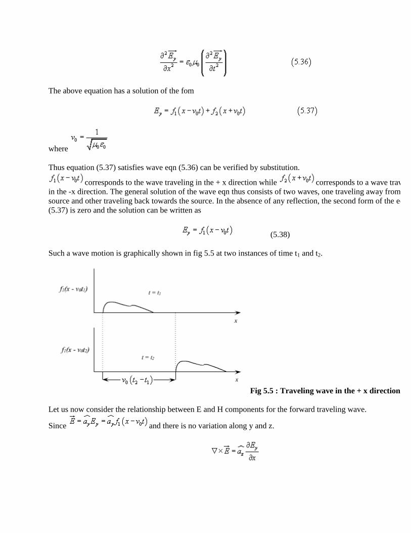
The above equation has a solution of the fom

where

Thus equation (5.37) satisfies wave eqn (5.36) can be verified by substitution.

corresponds to the wave traveling in the + x direction while corresponds to a wave traveling

in the -x direction. The general solution of the wave eqn thus consists of two waves, one traveling away from the

source and other traveling back towards the source. In the absence of any reflection, the second form of the eqn

(5.37) is zero and the solution can be written as

(5.38)

Such a wave motion is graphically shown in fig 5.5 at two instances of time t1 and t2.

Fig 5.5 : Traveling wave in the + x direction

Let us now consider the relationship between E and H components for the forward traveling wave.

Since and there is no variation along y and z.

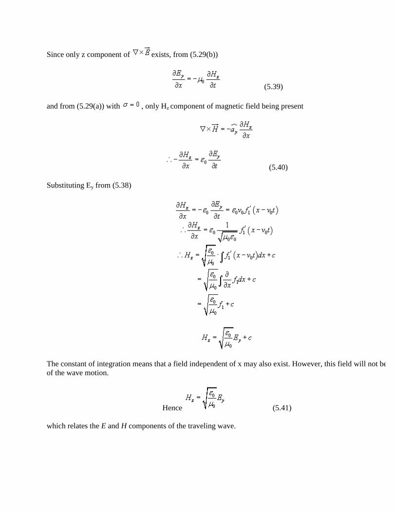
Since only z component of exists, from (5.29(b))

(5.39)

and from (5.29(a)) with , only Hz component of magnetic field being present

(5.40)

Substituting Ey from (5.38)

The constant of integration means that a field independent of x may also exist. However, this field will not be a part

of the wave motion.

Hence (5.41)

which relates the E and H components of the traveling wave.

is called the characteristic or intrinsic impedance of the free space

TIME HARMONIC FIELDS :

So far, in discussing time varying electromagnetic fields, we have considered arbitrary time dependence. The time

dependence of the field quantities depends on the source functions. One of the most important case of time varying

electromagnetic field is the time harmonic (sinusoidal or co sinusoidal) time variation where the excitation of the

source varies sinusoidally in time with a single frequency. For time-harmonic fields, phasor analysis can be applied

to obtain single frequency steady state response. Since Maxwell's equations are linear differential equations, for

source functions with arbitrary time dependence, electromagnetic fields can be determined by superposition.

Periodic time functions can be expanded into Fourier series of harmonic sinusoidal components while transient

non-periodic functions can be expressed as Fourier integrals. Field vectors that vary with space coordinates and are

sinusoidal function of time can be represented in terms of vector phasors that depend on the space coordinates but

not on time. For time harmonic case, the general time variation is and for a cosine reference, the instantaneous

fields can be written as:

(5.42)

where is a vector phasor that contain the information on direction, magnitude and phase. The phasors in

general are complex quantities. All time harmonic filed components can be written in this manner.

thus we find that if the electric field vector is represented in the phasor form as , then

can be represented by the phasor . The integral can be represented by the

phasor . In the same manner, higher order derivatives and integrals with respect to t can be represented

by multiplication and division of the phasor by higher power of . Considering the field phasors

and source phasors in a simple linear isotropic medium, we can write the Maxwell's equations for

time harmonic case in the phasor form as:

(5.4 4a)

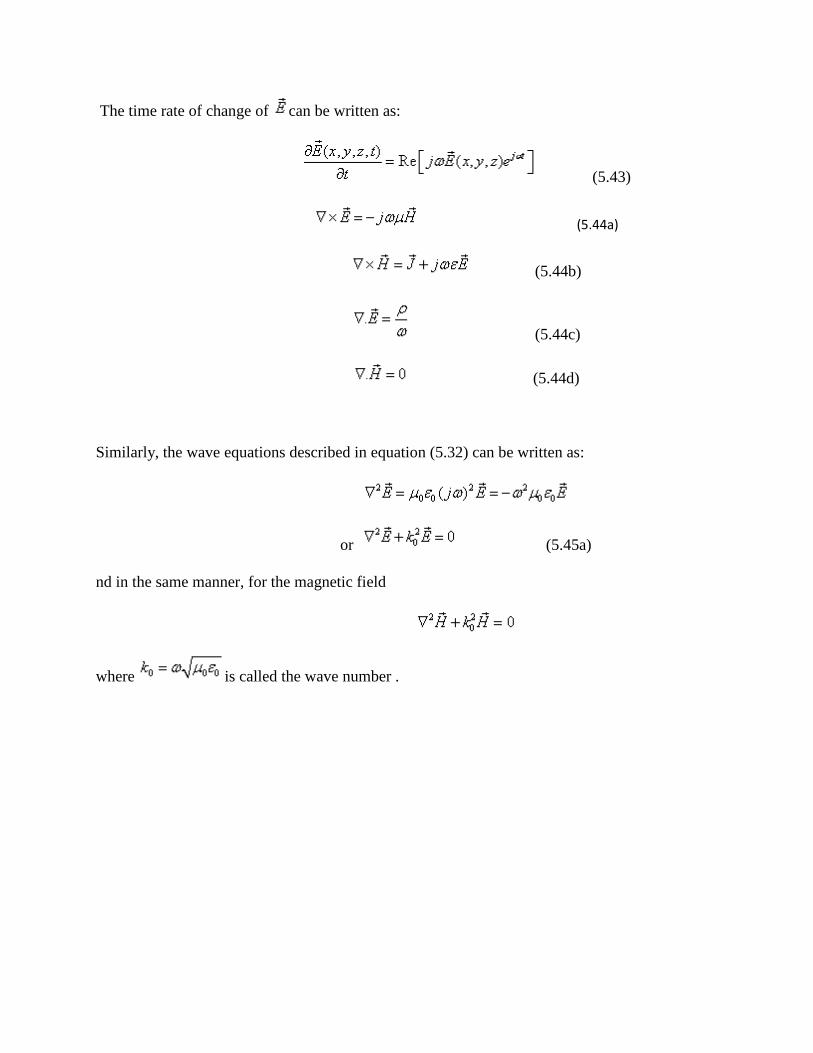
The time rate of change of can be written as:

(5.43)

(5.44a)

(5.44b)

(5.44c)

(5.44d)

Similarly, the wave equations described in equation (5.32) can be written as:

or (5.45a)

nd in the same manner, for the magnetic field

where is called the wave number .

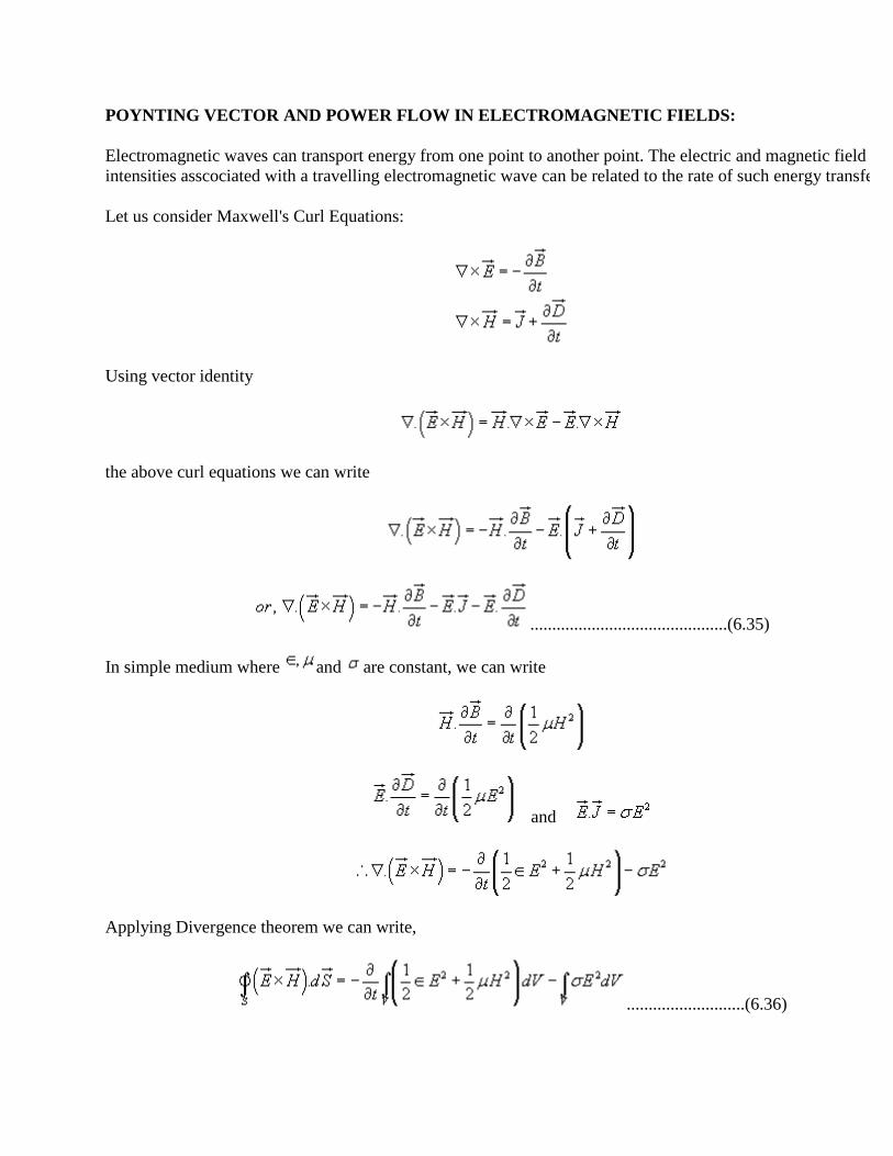
POYNTING VECTOR AND POWER FLOW IN ELECTROMAGNETIC FIELDS:

Electromagnetic waves can transport energy from one point to another point. The electric and magnetic field

intensities asscociated with a travelling electromagnetic wave can be related to the rate of such energy transfer.

Let us consider Maxwell's Curl Equations:

Using vector identity

the above curl equations we can write

.............................................(6.35)

In simple medium where and are constant, we can write

and

Applying Divergence theorem we can write,

...........................(6.36)

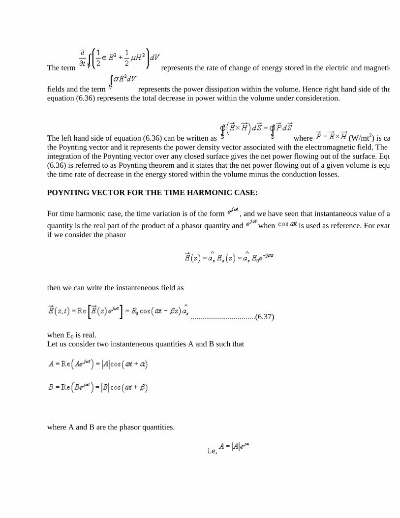
The term represents the rate of change of energy stored in the electric and magnetic

fields and the term represents the power dissipation within the volume. Hence right hand side of the

equation (6.36) represents the total decrease in power within the volume under consideration.

The left hand side of equation (6.36) can be written as where (W/mt2) is called

the Poynting vector and it represents the power density vector associated with the electromagnetic field. The

integration of the Poynting vector over any closed surface gives the net power flowing out of the surface. Equation

(6.36) is referred to as Poynting theorem and it states that the net power flowing out of a given volume is equal to

the time rate of decrease in the energy stored within the volume minus the conduction losses.

POYNTING VECTOR FOR THE TIME HARMONIC CASE:

For time harmonic case, the time variation is of the form , and we have seen that instantaneous value of a

quantity is the real part of the product of a phasor quantity and when is used as reference. For example,

if we consider the phasor

then we can write the instanteneous field as

.................................(6.37)

when E0 is real.

Let us consider two instanteneous quantities A and B such that

where A and B are the phasor quantities.

i.e,

Therefore,

..............................(6.39)

ince A and B are periodic with period , the time average value of the product form AB, denoted by can

be written as

.....................................(6.40)

Further, considering the phasor quantities A and B, we find that

and , where * denotes complex conjugate.

UNIT IV TIME VARYING ELECTRIC AND MAGNETIC FIELDS

PART- A (2 MARKS) 1. State Faraday’s law of induction . 2. State lenz’s law 3. Give the equation of transformer emf 4. What is motional electric field? 5. What is motinal emf ? 6. What is the emf produced by moving loop in time varying field? EE 1201 ELECTROMAGNETIC THEORY KINGS COLLEGE OF ENGINEERING, PUNALKULAM 6

7. What is time harmonic field ? 8. Give time harmonic maxwell’s equation in point form. assume time factor e-i_t. 9. Distingush between Field theory and Circuit theory 10. Write Maxwell’s equation in point and integral form for good conductors. 11. What Is significance of displacement current density? 12. In a material for which = 5s/m and _r= 1 and E=250 sin 1010t (V/m) find the conduction and displacement current densities.

PART- B 1. What are the different ways of EMF generation? Explain with the governing equations and suitable practical examples. (16) 2. With necessary explanation, derive the Maxwell’s equation in differential and integral forms (16) 3. (a) What do you mean by displacement current? write down the expression for the total current density (8) (b) In a material for which =5 s/m and _r=1 and E=250 sin 1010t (V/m).find the conduction and displacement current densities. (8) 4 .(a) Find the total current in a circular conductor of radius 4mm if the current density varies according to J=104/R A/m2 . (8) (b) Given the conduction current density in a lossy dielectric as Jc=0.02 sin 109 t A/m2 .find the displacement current density if =103 mho/m and _r=6.5 (8) 5 (a) Explain the relation between field theory and circuit theory. (8) (b)The magnetic field intensity in free space is given as H=H0sin_ ay t A/m. where _=_t-_z and _ is a constant quantity. Determine the displacement current density. (8) 6 (a) Write short notes on faradays law of electromagnetic induction. (8) (b) Show that the ratio of the amplitudes of the conduction current density and displacement current density is /__, for the applied field amplitude ratio if the applied field is E=Em e-t/_ where _ is real. (8) 7. Derive General field relation for time varying electric and magnetic fields using Maxwell’s’ equations. (16)

UNIT V ELECTROMAGNETIC WAVES

Derivation of wave equation – Uniform plane waves – Maxwell‟s equation in phasor

form – Wave equation in phasor form – Plane waves in free space and in a homogenous

material – Wave equation for a conducting medium – Plane waves in lossy dielectrics –

Propagation in good conductors – Skin effect – Linear elliptical and circular polarization

– Reflection of plane wave from a conductor – Normal incidence – Reflection of plane

Waves by a perfect dielectric – Normal and oblique incidence – Dependence on

polarization – Brewster angle.

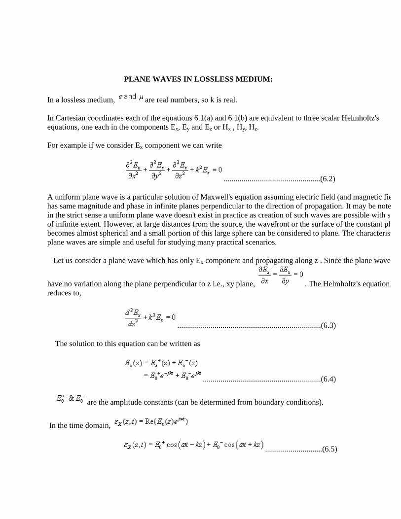
PLANE WAVES IN LOSSLESS MEDIUM:

In a lossless medium, are real numbers, so k is real.

In Cartesian coordinates each of the equations 6.1(a) and 6.1(b) are equivalent to three scalar Helmholtz's

equations, one each in the components Ex, Ey and Ez or Hx , Hy, Hz.

For example if we consider Ex component we can write

.................................................(6.2)

A uniform plane wave is a particular solution of Maxwell's equation assuming electric field (and magnetic field)

has same magnitude and phase in infinite planes perpendicular to the direction of propagation. It may be noted that

in the strict sense a uniform plane wave doesn't exist in practice as creation of such waves are possible with sources

of infinite extent. However, at large distances from the source, the wavefront or the surface of the constant phase

becomes almost spherical and a small portion of this large sphere can be considered to plane. The characteristics of

plane waves are simple and useful for studying many practical scenarios.

Let us consider a plane wave which has only Ex component and propagating along z . Since the plane wave will

have no variation along the plane perpendicular to z i.e., xy plane, . The Helmholtz's equation (6.2)

reduces to,

.........................................................................(6.3)

The solution to this equation can be written as

............................................................(6.4)

are the amplitude constants (can be determined from boundary conditions).

In the time domain,

.............................(6.5)

assuming are real constants.

Here, represents the forward traveling wave. The plot of for several values

of t is shown in the Figure 6.1.

Figure 6.1: Plane wave traveling in the + z direction

As can be seen from the figure, at successive times, the wave travels in the +z direction.

If we fix our attention on a particular point or phase on the wave (as shown by the dot) i.e. , = constant

Then we see that as t is increased to , z also should increase to so that

Or,

Or,

When ,

we write = phase velocity .

.....................................(6.6)

If the medium in which the wave is propagating is free space i.e.,

Then

Where 'C' is the speed of light. That is plane EM wave travels in free space with the speed of light.

The wavelength is defined as the distance between two successive maxima (or minima or any other reference

points).

i.e.,

or,

or,

Substituting ,

or, ................................(6.7)

Thus wavelength also represents the distance covered in one oscillation of the wave. Similarly,

represents a plane wave traveling in the -z direction.

The associated magnetic field can be found as follows:

From (6.4),

=

= ............(6.8)

where is the intrinsic impedance of the medium.

When the wave travels in free space

is the intrinsic impedance of the free space.

In the time domain,

........... (6.9)

Which represents the magnetic field of the wave traveling in the +z direction.

For the negative traveling wave,

...........(6.10)

For the plane waves described, both the E & H fields are perpendicular to the direction of propagation, and these

waves are called TEM (transverse electromagnetic) waves.

The E & H field components of a TEM wave is shown in Fig 6.2.

Figure 6.2 : E & H fields of a particular plane wave at time t.

PLANE WAVES IN A LOSSY MEDIUM :

In a lossy medium, the EM wave looses power as it propagates. Such a medium is conducting with conductivity

and we can write:

.....................(6.19)

Where is called the complex permittivity.

We have already discussed how an external electric field can polarize a dielectric and give rise to bound charges.

When the external electric field is time varying, the polarization vector will vary with the same frequency as that of

the applied field. As the frequency of the applied filed increases, the inertia of the charge particles tend to prevent

the particle displacement keeping pace with the applied field changes. This results in frictional damping mechanism

causing power loss.

In addition, if the material has an appreciable amount of free charges, there will be ohmic losses. It is customary to

include the effect of damping and ohmic losses in the imaginary part of . An equivalent conductivity

represents all losses.

The ratio is called loss tangent as this quantity is a measure of the power loss.

POLARISATION OF PLANE WAVE:

The polarisation of a plane wave can be defined as the orientation of the electric field vector as a function of time at

a fixed point in space. For an electromagnetic wave, the specification of the orientation of the electric field is

sufficent as the magnetic field components are related to electric field vector by the Maxwell's equations.

Let us consider a plane wave travelling in the +z direction. The wave has both Ex and Ey components.

..........................................(6.45)

The corresponding magnetic fields are given by,

Depending upon the values of Eox and Eoy we can have several possibilities:

1. If Eoy = 0, then the wave is linearly polarised in the x-direction.

2. If Eoy = 0, then the wave is linearly polarised in the y-direction.

3. If Eox and Eoy are both real (or complex with equal phase), once again we get a linearly polarised wave with the

axis of polarisation inclined at an angle , with respect to the x-axis. This is shown in fig 6.4.

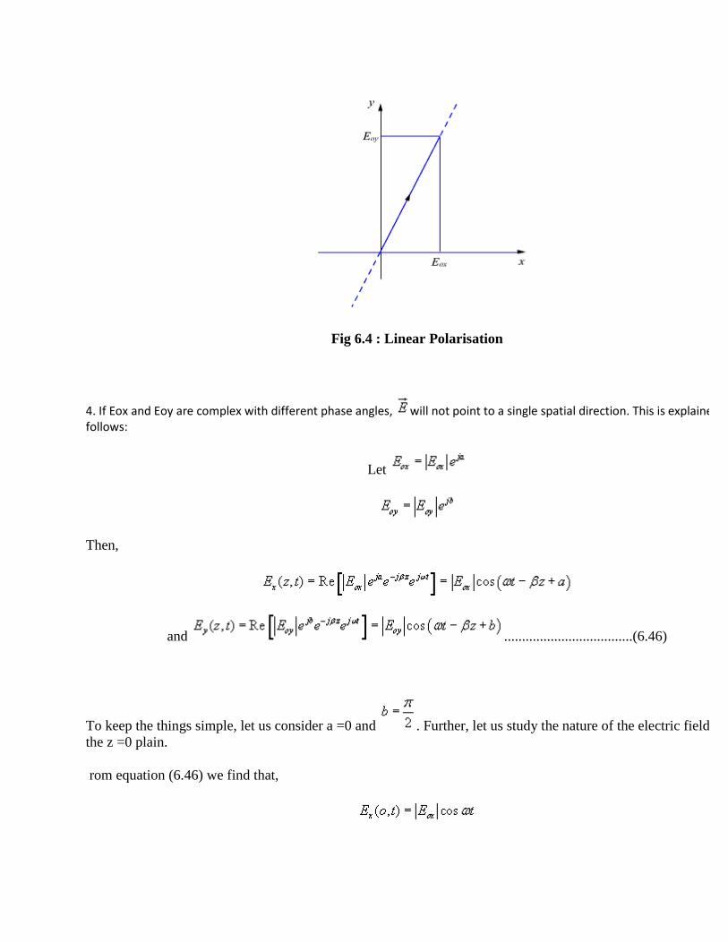
Fig 6.4 : Linear Polarisation

4. If Eox and Eoy are complex with different phase angles, will not point to a single spatial direction. This is explained as follows:

Let

Then,

and ....................................(6.46)

To keep the things simple, let us consider a =0 and . Further, let us study the nature of the electric field on

the z =0 plain.

rom equation (6.46) we find that,

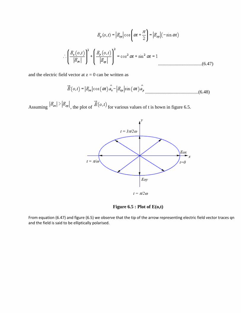
.....................................(6.47)

and the electric field vector at z = 0 can be written as

.............................................(6.48)

Assuming , the plot of for various values of t is hown in figure 6.5.

Figure 6.5 : Plot of E(o,t)

From equation (6.47) and figure (6.5) we observe that the tip of the arrow representing electric field vector traces qn ellipse and the field is said to be elliptically polarised.

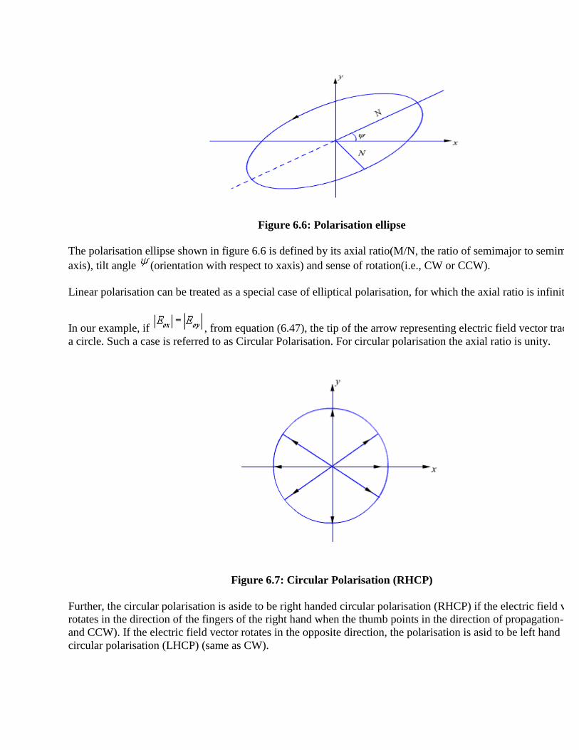
Figure 6.6: Polarisation ellipse

The polarisation ellipse shown in figure 6.6 is defined by its axial ratio(M/N, the ratio of semimajor to semiminor

axis), tilt angle (orientation with respect to xaxis) and sense of rotation(i.e., CW or CCW).

Linear polarisation can be treated as a special case of elliptical polarisation, for which the axial ratio is infinite.

In our example, if , from equation (6.47), the tip of the arrow representing electric field vector traces out

a circle. Such a case is referred to as Circular Polarisation. For circular polarisation the axial ratio is unity.

Figure 6.7: Circular Polarisation (RHCP)

Further, the circular polarisation is aside to be right handed circular polarisation (RHCP) if the electric field vector

rotates in the direction of the fingers of the right hand when the thumb points in the direction of propagation-(same

and CCW). If the electric field vector rotates in the opposite direction, the polarisation is asid to be left hand

circular polarisation (LHCP) (same as CW).

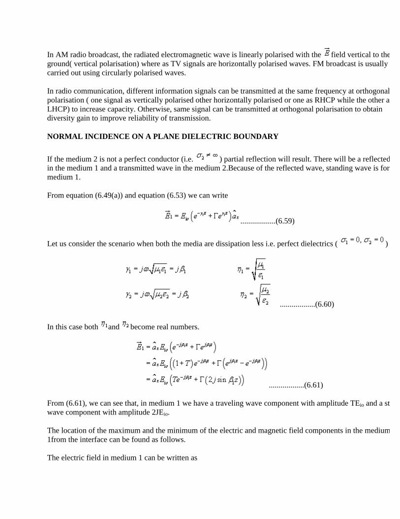
In AM radio broadcast, the radiated electromagnetic wave is linearly polarised with the field vertical to the

ground( vertical polarisation) where as TV signals are horizontally polarised waves. FM broadcast is usually

carried out using circularly polarised waves.

In radio communication, different information signals can be transmitted at the same frequency at orthogonal

polarisation ( one signal as vertically polarised other horizontally polarised or one as RHCP while the other as

LHCP) to increase capacity. Otherwise, same signal can be transmitted at orthogonal polarisation to obtain

diversity gain to improve reliability of transmission.

NORMAL INCIDENCE ON A PLANE DIELECTRIC BOUNDARY

If the medium 2 is not a perfect conductor (i.e. ) partial reflection will result. There will be a reflected wave

in the medium 1 and a transmitted wave in the medium 2.Because of the reflected wave, standing wave is formed in

medium 1.

From equation (6.49(a)) and equation (6.53) we can write

..................(6.59)

Let us consider the scenario when both the media are dissipation less i.e. perfect dielectrics ( )

..................(6.60)

In this case both and become real numbers.

..................(6.61)

From (6.61), we can see that, in medium 1 we have a traveling wave component with amplitude TEio and a standing

wave component with amplitude 2JEio.

The location of the maximum and the minimum of the electric and magnetic field components in the medium

1from the interface can be found as follows.

The electric field in medium 1 can be written as

..................(6.62)

If i.e. >0

The maximum value of the electric field is

..................(6.63)

and this occurs when

or , n = 0, 1, 2, 3.......................(6.64)

The minimum value of is

.................(6.65)

And this occurs when

or , n = 0, 1, 2, 3.............................(6.66)

For i.e. <0

The maximum value of is which occurs at the zmin locations and the minimum value of is

which occurs at zmax locations as given by the equations (6.64) and (6.66).

From our discussions so far we observe that can be written as

.................(6.67)

The quantity S is called as the standing wave ratio.

As the range of S is given by

From (6.62), we can write the expression for the magnetic field in medium 1 as

.................(6.68)

From (6.68) we find that will be maximum at locations where is minimum and vice versa.

In medium 2, the TRANSMITTED WAVE PROPAGATES IN THE + Z DIRECTION.

OBLIQUE INCIDENCE OF EM WAVE AT AN INTERFACE

So far we have discuss the case of normal incidence where electromagnetic wave traveling in a lossless medium

impinges normally at the interface of a second medium. In this section we shall consider the case of oblique

incidence. As before, we consider two cases

1. When the second medium is a perfect conductor.

2. When the second medium is a perfect dielectric.

A plane incidence is defined as the plane containing the vector indicating the direction of propagation of the

incident wave and normal to the interface. We study two specific cases when the incident electric field is

perpendicular to the plane of incidence (perpendicular polarization) and is parallel to the plane of incidence

(parallel polarization). For a general case, the incident wave may have arbitrary polarization but the same can be

expressed as a linear combination of these two individual cases.

Oblique Incidence at a plane conducting boundary

3. Perpendicular Polarization

The situation is depicted in figure 6.10.

Figure 6.10: Perpendicular Polarization

As the EM field inside the perfect conductor is zero, the interface reflects the incident plane wave. and

respectively represent the unit vector in the direction of propagation of the incident and reflected waves, is

the angle of incidence and is the angle of reflection.

We find that

............................(6.69)

Since the incident wave is considered to be perpendicular to the plane of incidence, which for the present case

happens to be xz plane, the electric field has only y-component.

Therefore,

The corresponding magnetic field is given by

...........................(6.70)

Similarly, we can write the reflected waves as

...................................................(6.71)

Since at the interface z=o, the tangential electric field is zero.

............................................(6.72)

Consider in equation (6.72) is satisfied if we have

..................................(6.73)

The condition is Snell's law of reflection.

..................................(6.74)

..................................(6.75)

The total electric field is given by

..................................(6.76)

Similarly, total magnetic field is given by

.............................(6.77)

From eqns (6.76) and (6.77) we observe that

4. Along z direction i.e. normal to the boundary

y component of and x component of maintain standing wave patterns according to and

where . No average power propagates along z as y component of and x component

of are out of phase.

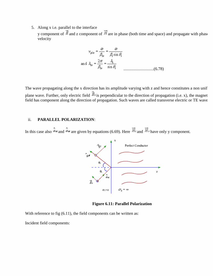
5. Along x i.e. parallel to the interface

y component of and z component of are in phase (both time and space) and propagate with phase

velocity

.............................(6.78)

The wave propagating along the x direction has its amplitude varying with z and hence constitutes a non uniform

plane wave. Further, only electric field is perpendicular to the direction of propagation (i.e. x), the magnetic

field has component along the direction of propagation. Such waves are called transverse electric or TE waves.

ii. PARALLEL POLARIZATION:

In this case also and are given by equations (6.69). Here and have only y component.

Figure 6.11: Parallel Polarization

With reference to fig (6.11), the field components can be written as:

Incident field components:

............................(6.79)

Reflected field components:

............................(6.80)

Since the total tangential electric field component at the interface is zero.

Which leads to and as before.

Substituting these quantities in (6.79) and adding the incident and reflected electric and magnetic field components

the total electric and magnetic fields can be written as

...........................(6.81)

Once again, we find a standing wave pattern along z for the x and y components of and , while a non uniform

plane wave propagates along x with a phase velocity given by where . Since, for this

propagating wave, magnetic field is in transverse direction, such waves are called transverse magnetic or TM

waves.

OBLIQUE INCIDENCE AT A PLANE DIELECTRIC INTERFACE

We continue our discussion on the behavior of plane waves at an interface; this time we consider a plane dielectric

interface. As earlier, we consider the two specific cases, namely parallel and perpendicular polarization.

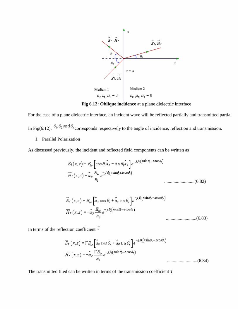
Fig 6.12: Oblique incidence at a plane dielectric interface

For the case of a plane dielectric interface, an incident wave will be reflected partially and transmitted partially.

In Fig(6.12), corresponds respectively to the angle of incidence, reflection and transmission.

1. Parallel Polarization

As discussed previously, the incident and reflected field components can be written as

..........................(6.82)

..........................(6.83)

In terms of the reflection coefficient

..........................(6.84)

The transmitted filed can be written in terms of the transmission coefficient T

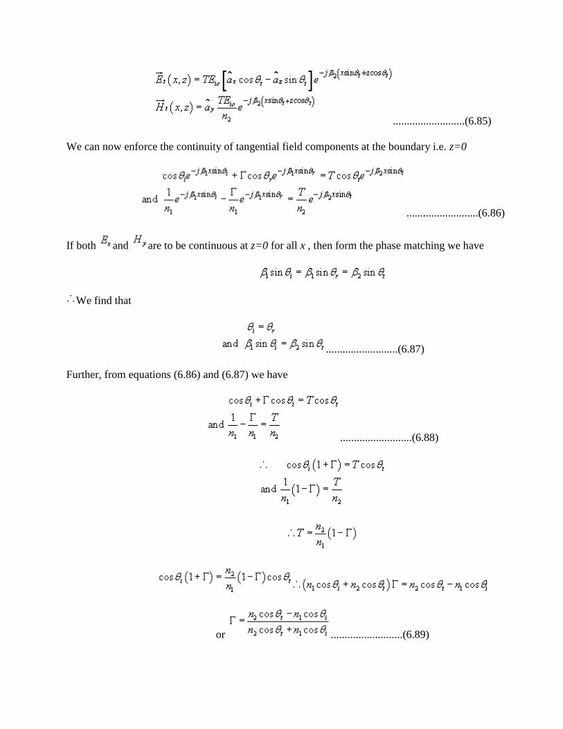
..........................(6.85)

We can now enforce the continuity of tangential field components at the boundary i.e. z=0

..........................(6.86)

If both and are to be continuous at z=0 for all x , then form the phase matching we have

We find that

..........................(6.87)

Further, from equations (6.86) and (6.87) we have

..........................(6.88)

or ..........................(6.89)

..........................(6.90)

From equation (6.90) we find that there exists specific angle for which = 0 such that

or .........................(6.91)

Further, .........................(6.92)

For non magnetic material

Using this condition

.........................(6.93)

From equation (6.93), solving for we get

This angle of incidence for which = 0 is called Brewster angle. Since we are dealing with parallel polarization we

represent this angle by so that

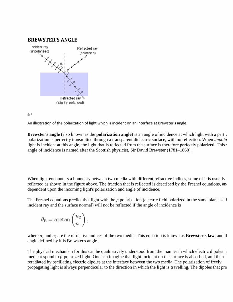
BREWSTER'S ANGLE

An illustration of the polarization of light which is incident on an interface at Brewster's angle.

Brewster's angle (also known as the polarization angle) is an angle of incidence at which light with a particular

polarization is perfectly transmitted through a transparent dielectric surface, with no reflection. When unpolarized

light is incident at this angle, the light that is reflected from the surface is therefore perfectly polarized. This special

angle of incidence is named after the Scottish physicist, Sir David Brewster (1781–1868).

When light encounters a boundary between two media with different refractive indices, some of it is usually

reflected as shown in the figure above. The fraction that is reflected is described by the Fresnel equations, and is

dependent upon the incoming light's polarization and angle of incidence.

The Fresnel equations predict that light with the p polarization (electric field polarized in the same plane as the

incident ray and the surface normal) will not be reflected if the angle of incidence is

where n1 and n2 are the refractive indices of the two media. This equation is known as Brewster's law, and the

angle defined by it is Brewster's angle.

The physical mechanism for this can be qualitatively understood from the manner in which electric dipoles in the

media respond to p-polarized light. One can imagine that light incident on the surface is absorbed, and then

reradiated by oscillating electric dipoles at the interface between the two media. The polarization of freely

propagating light is always perpendicular to the direction in which the light is travelling. The dipoles that produce

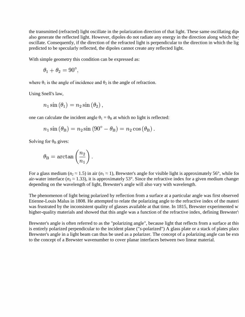
the transmitted (refracted) light oscillate in the polarization direction of that light. These same oscillating dipoles

also generate the reflected light. However, dipoles do not radiate any energy in the direction along which they

oscillate. Consequently, if the direction of the refracted light is perpendicular to the direction in which the light is

predicted to be specularly reflected, the dipoles cannot create any reflected light.

With simple geometry this condition can be expressed as:

where θ1 is the angle of incidence and θ2 is the angle of refraction.

Using Snell's law,

one can calculate the incident angle θ1 = θB at which no light is reflected:

Solving for θB gives:

For a glass medium (n2 ≈ 1.5) in air (n1 ≈ 1), Brewster's angle for visible light is approximately 56°, while for an

air-water interface (n2 ≈ 1.33), it is approximately 53°. Since the refractive index for a given medium changes

depending on the wavelength of light, Brewster's angle will also vary with wavelength.

The phenomenon of light being polarized by reflection from a surface at a particular angle was first observed by

Etienne-Louis Malus in 1808. He attempted to relate the polarizing angle to the refractive index of the material, but

was frustrated by the inconsistent quality of glasses available at that time. In 1815, Brewster experimented with

higher-quality materials and showed that this angle was a function of the refractive index, defining Brewster's law.

Brewster's angle is often referred to as the "polarizing angle", because light that reflects from a surface at this angle

is entirely polarized perpendicular to the incident plane ("s-polarized") A glass plate or a stack of plates placed at

Brewster's angle in a light beam can thus be used as a polarizer. The concept of a polarizing angle can be extended

to the concept of a Brewster wavenumber to cover planar interfaces between two linear material.

UNIT V ELECTROMAGNETIC WAVES PART- A (2 MARKS) 1. Define a Wave. 2. Mention the properties of uniform plane wave. 3. Write down the wave equation for E and H in free space. 4. Write down the wave equation for E and H in a conducting medium 5. Define intrinsic impedance or characteristic impedance. 6. Calculate the characteristic impedance of free space. 7. Define propagation constant. 8. Define skin depth 9. Define Pointing vector. 10. State Poynting Theorem. 11. What is lossy dielectric medium? 12. For a loss dielectric material having μr=1 ,_ r=48, =20s/m. calculate the Propagation constant at a frequency of 16 GHz 13. Define Polarization 14. Define Circular Polarization 15. Define Elliptical polarization 16. Define Linear Polarization

PART- B 1. (a) Calculate the attenuation constant and phase constant for the uniform plane wave with the frequency of 10GHz in a medium for which μ=μ0, _r=2.3 and =2.54x10-4_/m (8) (b) Derive the expression for the attenuation constant ,phase constant and intrinsic impedance for a uniform plane wave in a good conductor. (8) 2. Derive the one dimensional general wave equation and find the solution for wave equation. (16) 3. Discuss about the plane waves in lossy dielectrics. (16) 4. Discuss about the plane waves in lossless dielectrics. (16) 5. Briefly explain about the wave incident (i) Normally on perfect conductor (8) (ii) Obliquely to the surface of perfect conductor. ( 6. (a). Assume that Eland H waves, traveling in free space, are normally Incident on the interface with a perfect dielectric with _r=3 .calculate the magnitudes of incident, reflected and transmitted E and H waves at the interface. (8) (b) A uniform plane wave of 200 MHz, traveling in free space Impinges normally on a large block of material having _r =4 , μr =9 and =0. Calculate transmission and reflection co efficient of interface. (8)

7. Derive wave equation in phasor form and also derive for __ _and _ (16) 8. Derive suitable relations for integral and point forms of poynting theorem. (16) 9. A plane wave propagating through a medium with _r = 8, μr = 2 has E = 0.5 sin (108 t – _z ) az V/m. Determine (i) _ (ii) The loss tangent (iii) Wave impedance (iv) Wave velocity (V) H field (16)