Ebs Cohost
60
5 ROCK MASS MODEL Antonio Karzulovic and John Read 5.1 Introduction Chapters 3 and 4 dealt with the geological and structural components of the geotechnical model. The third component, which must now be addressed, is the rock mass model (Figure 5.1). The purpose of this model is to database the engineering properties of the rock mass for use in the stability analyses that will be used to prepare the slope designs at each stage of project development. This includes the properties of the intact pieces of rock that constitute the anisotropic rock mass, the structures that cut through the rock mass and separate the individual pieces of intact rock from each other, and the rock mass itself. As outlined in Chapter 10 (section 10.1.1), when assessing potential failure mechanisms of any rock mass a fundamental attribute that must always be considered is that in stronger rocks structure is likely to be the primary control, whereas in weaker rocks strength can be the controlling factor. This means that the rock mass may fail in three possible ways: 1 structurally controlled failure, where the rupture occurs only along the joints, bedding or faults. This is the case for planar and wedge slides, which are most likely to occur at bench and inter-ramp scale. In this case the strength and orientation of the structures are the most important parameters in assessing slope stability; 2 failure with partial structural control, where rupture occurs partly through the rock mass and partly through the structures, usually at inter-ramp and overall scale. In this case the strength of the rock mass and the strength and orientation of the structures are both important in assessing slope stability; 3 failure with limited structural control, where the rupture occurs predominantly through the rock mass. This can occur at inter-ramp or overall slope scale in either highly fractured or weak rock masses mostly comprising soft or altered material. In this case the strength of the rock mass is the most important parameter in assessing slope stability. Hence, when setting out to determine the geotechnical engineering properties of the rock mass, the strength of the rock mass and the potential mechanism of failure must be considered and factored into the sampling and testing program. Data representative of the intact pieces of rock, the structures and the rock mass itself will all be required at some stage of the slope design and must be incorporated in the rock mass model. The procedures involved in gathering these data are the focus of the next four sections. Section 5.2 deals with the properties of the intact rock. It outlines the nature of the standard index and mechanical property tests used in rock slope engineering (sections 5.2.1, 5.2.2 and 5.2.3) then outlines testing needs for special cases such as weak, saprolitic and/or highly weathered and altered rocks, degradable clay shales and permafrost conditions (section 5.2.4). Section 5.3 deals with the strength of the mechanical defects in the rock mass, especially shear strength and the effects of surface roughness. Section 5.4 outlines the methods currently used to classify the rock mass. Section 5.5 completes the chapter, with descriptions of current and newly developed means of assessing the strength of the rock mass. 5.2 Intact rock strength 5.2.1 Introduction The geomechanical properties of the intact rock that occurs between the structural defects in a typical rock mass are measured in the laboratory from representative samples of the intact rock. The need to obtain representative samples is important. For example, it is not uncommon that only the ‘best’ core samples are sent to the laboratory for uniaxial compression testing, which can Copyright © 2009. CSIRO Pub. All rights reserved. May not be reproduced in any form without permission from the publisher, except fair uses permitted under U.S. or applicable copyright law. EBSCO Publishing : eBook Collection (EBSCOhost) - printed on 3/4/2015 11:58 AM via UNIVERSIDAD DE SONORA AN: 390201 ; Read, John, Stacey, Peter.; Guidelines for Open Pit Slope Design Account: s4090146
-
Upload
gustavo-rios -
Category
Documents
-
view
25 -
download
0
description
mecanica de rocas
Transcript of Ebs Cohost
5 ROCK MASS MODELAntonio Karzulovic and John Read
5.1 IntroductionChapters 3 and 4 dealt with the geological and structural components of the geotechnical model. The third component, which must now be addressed, is the rock mass model (Figure 5.1). The purpose of this model is to database the engineering properties of the rock mass for use in the stability analyses that will be used to prepare the slope designs at each stage of project development. This includes the properties of the intact pieces of rock that constitute the anisotropic rock mass, the structures that cut through the rock mass and separate the individual pieces of intact rock from each other, and the rock mass itself.
As outlined in Chapter 10 (section 10.1.1), when assessing potential failure mechanisms of any rock mass a fundamental attribute that must always be considered is that in stronger rocks structure is likely to be the primary control, whereas in weaker rocks strength can be the controlling factor. This means that the rock mass may fail in three possible ways:
1 structurally controlled failure, where the rupture occurs only along the joints, bedding or faults. This is the case for planar and wedge slides, which are most likely to occur at bench and inter-ramp scale. In this case the strength and orientation of the structures are the most important parameters in assessing slope stability;
2 failure with partial structural control, where rupture occurs partly through the rock mass and partly through the structures, usually at inter-ramp and overall scale. In this case the strength of the rock mass and the strength and orientation of the structures are both important in assessing slope stability;
3 failure with limited structural control, where the rupture occurs predominantly through the rock mass. This can occur at inter-ramp or overall slope scale in either highly fractured or weak rock masses mostly comprising soft or altered material. In this case the
strength of the rock mass is the most important parameter in assessing slope stability.
Hence, when setting out to determine the geotechnical engineering properties of the rock mass, the strength of the rock mass and the potential mechanism of failure must be considered and factored into the sampling and testing program. Data representative of the intact pieces of rock, the structures and the rock mass itself will all be required at some stage of the slope design and must be incorporated in the rock mass model. The procedures involved in gathering these data are the focus of the next four sections.
Section 5.2 deals with the properties of the intact rock. It outlines the nature of the standard index and mechanical property tests used in rock slope engineering (sections 5.2.1, 5.2.2 and 5.2.3) then outlines testing needs for special cases such as weak, saprolitic and/or highly weathered and altered rocks, degradable clay shales and permafrost conditions (section 5.2.4).
Section 5.3 deals with the strength of the mechanical defects in the rock mass, especially shear strength and the effects of surface roughness. Section 5.4 outlines the methods currently used to classify the rock mass. Section 5.5 completes the chapter, with descriptions of current and newly developed means of assessing the strength of the rock mass.
5.2 Intact rock strength5.2.1 IntroductionThe geomechanical properties of the intact rock that occurs between the structural defects in a typical rock mass are measured in the laboratory from representative samples of the intact rock. The need to obtain representative samples is important. For example, it is not uncommon that only the ‘best’ core samples are sent to the laboratory for uniaxial compression testing, which can Co
pyright © 2009. CSI
RO Pub. All rights reserved. May not be reproduced in any form without permission from the publisher, except fair uses permitted under U.S. or applicable
copyright law.
EBSCO Publishing : eBook Collection (EBSCOhost) - printed on 3/4/2015 11:58 AM via UNIVERSIDAD DE SONORAAN: 390201 ; Read, John, Stacey, Peter.; Guidelines for Open Pit Slope DesignAccount: s4090146

Guidelines for Open Pit Slope Design84
result in the rock strength being overestimated. If the results of the tests show a large variation or, for example, there is only partial core recovery, it may be better not to consider a unique value such as the mean or the mode, but a range defined by upper and lower values. In the case of only partial recovery, the upper bound would be represented by the uniaxial strength of the ‘good’ core and the lower bound, representing the zones of core loss, would represent zones of significantly reduced strength.
When sampling and testing the intact rock it is also important to differentiate between ‘index’, ‘conductivity’ and ‘mechanical’ properties.
■ Index properties, which do not define the mechanical behaviour of the rock, but are easy to measure and provide a qualitative description of the rock and, in some cases, can be related to rock conductivity and/or mechanical properties. For example, an increase in rock porosity could explain a decrease in its strength.
■ Conductivity properties are properties that describe fluid flow through the rock. An example is hydraulic conductivity.
■ Mechanical properties are properties that describe quantitatively the strength and deformability of the rock. The most common example is uniaxial compres-
MODELS
DOMAINS
DESIGN
ANALYSES
IMPLEMENTATION
Geology
Equipment
Structure Rock Mass Hydrogeology
GeotechnicalModel
GeotechnicalDomains
StructureStrength
BenchConfigurations
Inter-RampAngles
Overall Slopes
FinalDesigns
Closure
Capabilities
Mine Planning
RiskAssessment
Depressurisation
Monitoring
Regulations
Blasting
Dewatering
Structure
Strength
Groundwater
In-situ Stress
Implementation
Failure Modes
Design Sectors
StabilityAnalysis
Partial Slopes
Overall Slopes
Movement
Design Model
INTE
RA
CTI
VE
PRO
CES
S
Figure 5.1: Slope design process
Copyright © 2009. CSI
RO Pub. All rights reserved. May not be reproduced in any form without permission from the publisher, except fair uses permitted under U.S. or applicable
copyright law.
EBSCO Publishing : eBook Collection (EBSCOhost) - printed on 3/4/2015 11:58 AM via UNIVERSIDAD DE SONORAAN: 390201 ; Read, John, Stacey, Peter.; Guidelines for Open Pit Slope DesignAccount: s4090146

Rock Mass Model 85
sive strength, which is one of the most used parameters in rock engineering.
Comprehensive discussions on rock properties and their measurement can be found in Lama et al. (1974), Lama and Vutukuri (1974), Farmer (1983), Nagaraj (1993), Bell (2000) and Zhang (2005).
In open pit slope engineering the most commonly used rock properties are the following.
■ Index properties (see section 5.2.2): → Point load strength index, I
s;
→ Porosity, n; → Unit weight, g; → P-wave velocity, V
P;
→ S-wave velocity, VS;
■ Mechanical properties (see section 5.2.3): → Tensile strength, TS or s
t;
→ Uniaxial compressive strength, UCS or sc;
→ Triaxial compressive strength, TCS; → Young’s modulus, E, and Poisson’s ratio, v.
5.2.2 Index properties5.2.2.1 Point load strength indexThe point load strength index, I
s, is an indirect estimate of
the uniaxial compressive strength of rock. The point load test can be performed on specimens in the form of core (diametral and axial tests), cut blocks (block tests) or irregular lumps (irregular lump test). The samples are broken by a concentrated load applied through a pair of spherically truncated, conical platens. The test can be performed in the field with portable equipment, or in the laboratory. The point load strength index, I
s, is given by:
IDP
se2= (eqn 5.1)
where P is the load that breaks the specimen and De is an
equivalent core diameter, given by:
D De= (eqn 5.2a)
D A4e p= for axial, block and lump tests
(eqn 5.2b)
where D is the core diameter and A is the minimum cross-sectional area of a plane through the specimen and the platen contact points. I
s varies with D
e. Hence, it is
preferable to carry out diametral tests on 50–55 mm diameter specimens.
Brady and Brown (2004) indicated that the value of Is
measured for a diameter De can be converted into an
equivalent 50 mm core Is by the relation:
I ID
50
.
s s De
e0 45
#= d]
ng (eqn 5.3)
where Is(De)
is the point load strength index measured for an equivalent core diameter D
e different from 50 mm. It is
not recommended to use core diameters smaller than 40 mm for point load testing (Bieniawski 1984).
Several correlations have been developed to estimate the uniaxial compressive strength of rock, s
c, from the
point load strength index (Zhang 2005), but the most commonly used is:
22 24 Itoc s
#.s ] g (eqn 5.4)
where Is is the point load strength index for D
e = 50 mm.
It should be noted that the point load test is not generally applicable for rocks with a CICS value below 25 MPa (R2 and lower), since the points tend to indent the rock. Further, extreme caution must be exercised when carrying out point load tests and interpreting the results using correlations such as Equation 5.4. First, there is considerable anecdotal and documented evidence that suggests there is no unique conversion factor and that it is necessary to determine the conversion factor on a site-by-site and rock type by rock type basis (Tsiambaos & Sabatakakis 2004). Second, as noted by Brady and Brown (2004), the test is one in which the fracture is caused by induced tension and it is essential that a consistent mode of failure be produced if the results obtained from different specimens are to be comparable. Very soft rocks and highly anisotropic rocks or rocks containing marked planes of weakness such as bedding planes are likely to give spurious results. A large degree of scatter is a general feature of point load test results and large numbers of individual determinations, often in excess of 100, are required in order to obtain reliable indices. For anisotropic rocks, it is usual to determine a strength anisotropy index, I
a, defined as the ratio of the mean I
s
values measured perpendicular and parallel to the planes of weakness.
ASTM Designation D5731-95 describes the standard test method for determination of the point load strength index of rock and Franklin (1985) describes the method suggested by the ISRM for determining point load strength.
5.2.2.2 PorosityThe porosity of rock, n, is defined as the proportion of the volume of voids (V
V) to the total volume (V
T) of the
sample. Porosity is traditionally expressed as a percentage.
nV
V
T
V= (eqn 5.5)
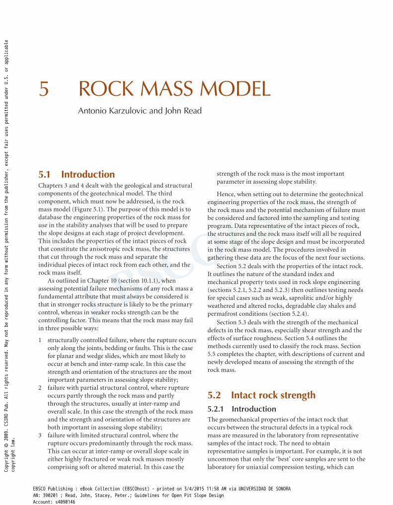
Goodman (1989) indicates that in sedimentary rocks n varies from close to 0 to as much as 90%, depending on the degree of consolidation or cementation, with 15% being a ‘typical’ value for an ‘average’ sandstone. Chalk is among the most porous of all rocks, with porosities in
Copyright © 2009. CSI
RO Pub. All rights reserved. May not be reproduced in any form without permission from the publisher, except fair uses permitted under U.S. or applicable
copyright law.
EBSCO Publishing : eBook Collection (EBSCOhost) - printed on 3/4/2015 11:58 AM via UNIVERSIDAD DE SONORAAN: 390201 ; Read, John, Stacey, Peter.; Guidelines for Open Pit Slope DesignAccount: s4090146
Guidelines for Open Pit Slope Design86
Table 5.1: Porosities of some rocks
Rock Type Rock Age Depth (m) n (%)
Chalk Chalk, Great Britain Cretaceous Surface 28.8
Diabase Frederick diabase – – 0.1
Dolomite Beekmantown dolomite Ordovician 3200 0.4
Niagara dolomite Silurian Surface 2.9
Gabbro San Marcos gabbro – – 0.2
Granite Granite, fresh – Surface 0–1
Granite, weathered – – 1–5
Granite, decomposed (saprolite)
– – 20
Limestone Black River limestone Ordovician Surface 0.46
Bedford limestone Mississippian Surface 12
Bermuda limestone Recent Surface 43
Dolomitic limestone – – 2.08
Limestone, Great Britain Carboniferous Surface 5.7
Limestone, Great Britain Silurian – 1.0
Oolitic limestone – – 1.06
Salem limestone Mississippian Surface 13.2
Solenhoffen limestone – Surface 4.8
Marble Marble – – 0.3
Marble – – 1.1
Mudstone Mudstone, Japan Upper Tertiary Near surface 22–32
Quartzite Quartzite, Great Britain Cambrian – 1.7–2.2
Sandstone Berea sandstone Mississippian 0-610 14
Keuper sandstone (England) Triassic Surface 22
Montana sandstone Cretaceous Surface 34
Mount Simon sandstone Cambrian 3960 0.7
Navajo sandstone Jurassic Surface 15.5
Nugget sandstone (Utah) Jurassic – 1.9
Potsdam sandstone Cambrian Surface 11
Pottsville sandstone Pennsylvanian – 2.9
Shale Shale Pre-Cambrian Surface 1.6
Shale Cretaceous 180 33.5
Shale Cretaceous 760 25.4
Shale Cretaceous 1065 21.1
Shale Cretaceous 1860 7.6
Shale Oklahoma Pennsylvanian 305 17
Shale Oklahoma Pennsylvanian 915 7
Shale Oklahoma Pennsylvanian 1525 4
Shale, Great Britain Silurian – 1.3–20
Tuff Tuff, bedded – – 40
Tuff, welded – – 14
Tonalite Cedar City tonalite – – 7
Source: Modified from Goodman (1989). Data selected from Clark (1966), Duncan (1969), Brace & Riley (1972)
Copyright © 2009. CSI
RO Pub. All rights reserved. May not be reproduced in any form without permission from the publisher, except fair uses permitted under U.S. or applicable
copyright law.
EBSCO Publishing : eBook Collection (EBSCOhost) - printed on 3/4/2015 11:58 AM via UNIVERSIDAD DE SONORAAN: 390201 ; Read, John, Stacey, Peter.; Guidelines for Open Pit Slope DesignAccount: s4090146

Rock Mass Model 87
some instances of more than 50%. Some volcanic materials, e.g. pumice and tuff, were well-aerated as they were formed and can also present very high porosities, but most magma-derived volcanic rocks have a low porosity. Crystalline rocks, including limestones and evaporites and most igneous and metamorphic rocks, also have low porosities, with a large proportion of the void space often being created by planar cracks or fissures. In these rocks n is usually less than 1–2% unless weathering has taken hold. As weathering progresses, n can increase well beyond 2%.
The ISRM-recommended procedures for measuring the porosity of rock are described in ISRM (2007). A detailed discussion of porosity can be found in Lama and Vutukuri (1978). The porosities of some rocks are given in Table 5.1.
5.2.2.3 Unit weight
The unit weight of rock, g, is defined as ratio between the weight (W) and the total volume (V
T) of the sample:
VW
T
g = (eqn 5.6)
The density of rock, r, is defined as ratio between the mass (M) and the total volume (V
T) of rock:
VM
T
r = (eqn 5.7)
The specific gravity of rock, Gs, is defined as the ratio
between its unit weight (g) and the unit weight of water (g
w):
Gs
wgg
= (eqn 5.8)
The ISRM-recommended procedures for measuring the unit weight of rock are described in ISRM (2007). A detailed discussion of unit weight can be found in Lama and Vutukuri (1978). The unit weights of some rocks are given in Table 5.2.
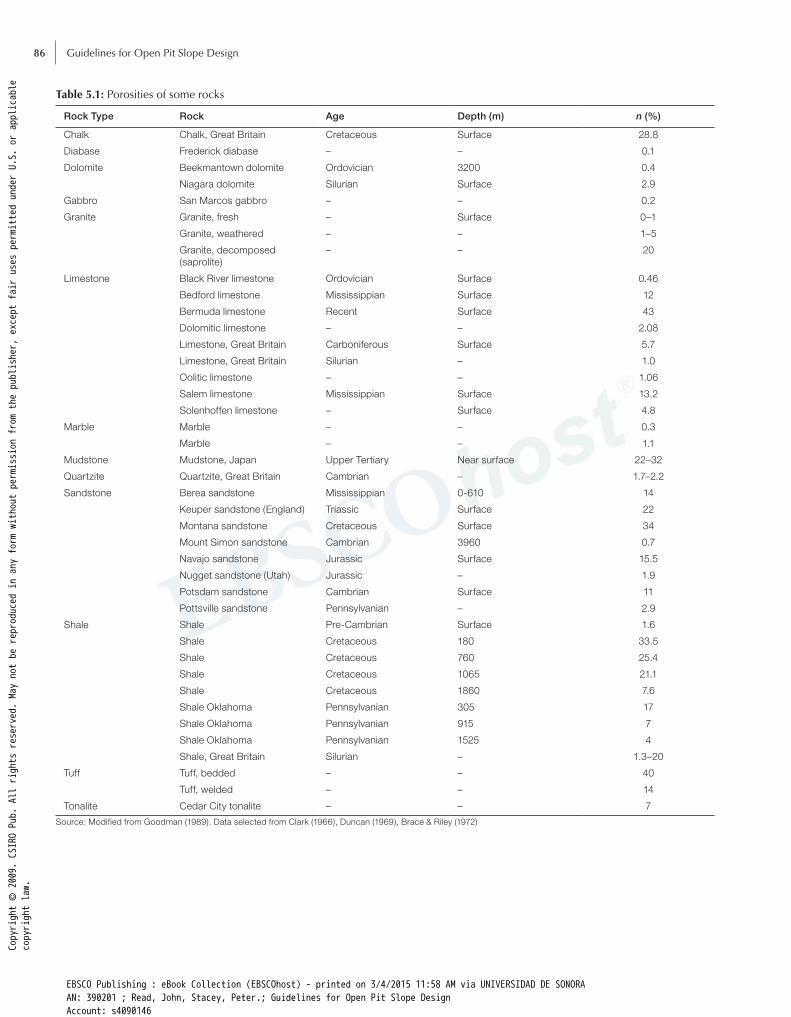
5.2.2.4 Wave velocityThe velocity of elastic waves in rock can be measured in the laboratory. Wave velocity is one of the most used index properties of rock and has been correlated with other index and mechanical properties of rock (Zhang 2005). Laboratory P-wave velocities vary from less than 1 km/sec in porous rocks to more than 6 km/sec in hard rocks.
Table 5.2: Dry unit weight of some rocks
Rock type g (kN/m3) g (tonne/m3) Rock type g (kN/m3) g (tonne/m3)
Amphibolite 27.0–30.9 2.75–3.15 Dolomite 26.0–27.5 2.65–2.80
Andesite 21.6–27.5 2.20–2.80 Limestone 23.1–27.0 2.35–2.75
Basalt 21.6–27.4 2.20–2.80 Marble 24.5–28.0 2.50–2.85
Chalk 21.6–24.5 2.20–2.50 Norite 26.5–29.4 2.70–3.00
Diabase 27.5–30.4 2.80–3.10 Peridotite 30.9–32.4 3.15–3.30
Diorite 26.5–28.9 2.70–2.95 Quartzite 25.5–26.5 2.60–2.70
Gabbro 26.5–30.4 2.70–3.10 Rock salt 20.6–21.6 2.10–2.20
Gneiss 25.5–30.9 2.60–3.15 Rhyolite 23.1–26.0 2.35–2.65
Granite 24.5–27.4 2.50–2.80 Sandstone 18.6–26.5 1.90–2.70
Granodiorite 26.0–27.5 2.65–2.80 Shale 19.6–26.0 2.00–2.65
Greywacke 26.0–26.5 2.65–2.70 Schist 25.5–29.9 2.60–3.05
Gypsum 22.1–23.1 2.25–2.35 Slate 26.5–28.0 2.70–2.85
Diorite 26.5–28.9 2.70–2.95 Syenite 25.5–28.4 2.60–2.90
Source: Data selected from Krynine & Judd (1957), Lama & Vutukuri (1978), Jumikis (1983), Carmichael (1989), Goodman (1989)
Table 5.3: Average P-wave velocities in rock-forming minerals
Mineral VP (m/sec) Mineral VP (m/sec) Mineral VP (m/sec)
Amphibole 7200 Epidote 7450 Olivine 8400
Augite 7200 Gypsum 5200 Orthoclase 5800
Biotite 5260 Hornblende 6810 Plagioclase 6250
Calcite 6600 Magnetite 7400 Pyrite 8000
Dolomite 7500 Muscovite 5800 Quartz 6050
Source: Data selected from Fourmaintraux (1976), Carmichael (1989)
Copyright © 2009. CSI
RO Pub. All rights reserved. May not be reproduced in any form without permission from the publisher, except fair uses permitted under U.S. or applicable
copyright law.
EBSCO Publishing : eBook Collection (EBSCOhost) - printed on 3/4/2015 11:58 AM via UNIVERSIDAD DE SONORAAN: 390201 ; Read, John, Stacey, Peter.; Guidelines for Open Pit Slope DesignAccount: s4090146
Guidelines for Open Pit Slope Design88
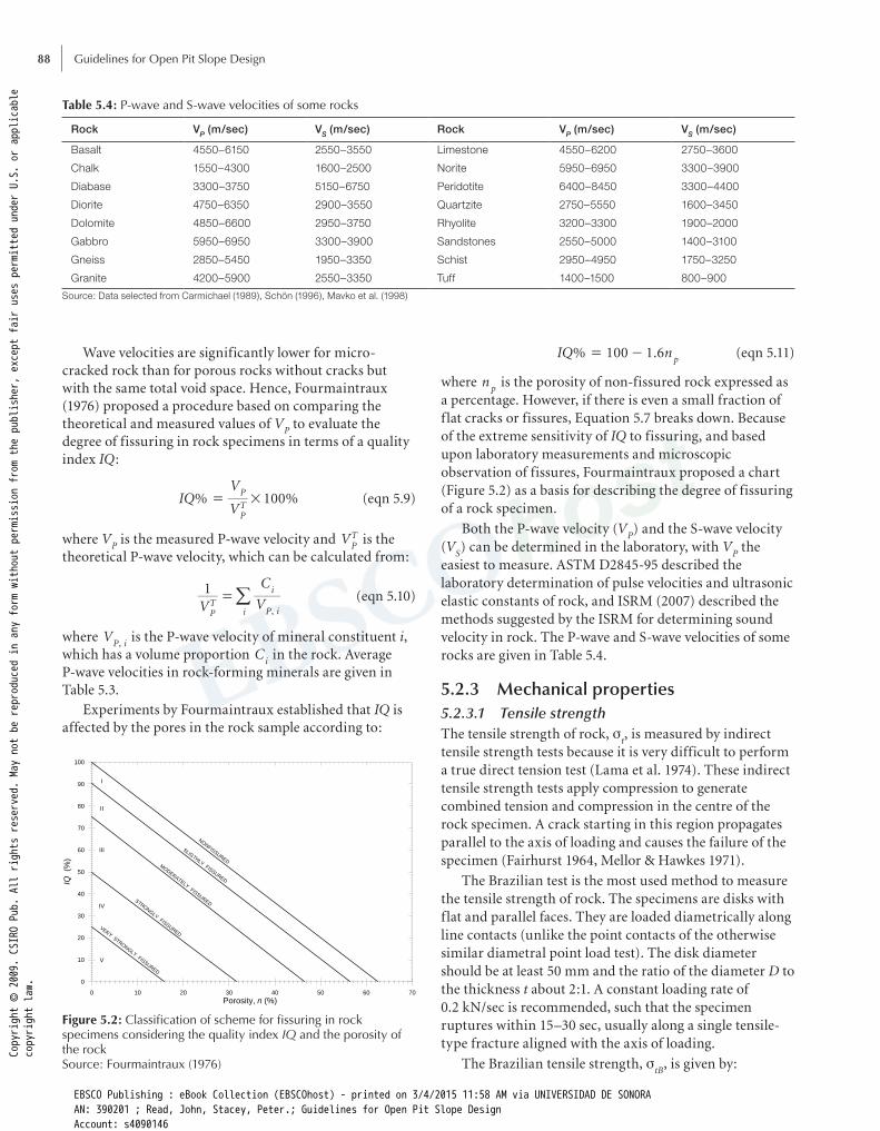
Wave velocities are significantly lower for micro-cracked rock than for porous rocks without cracks but with the same total void space. Hence, Fourmaintraux (1976) proposed a procedure based on comparing the theoretical and measured values of V
P to evaluate the
degree of fissuring in rock specimens in terms of a quality index IQ:
% %IQV
V100
PT
P#= (eqn 5.9)
where VP is the measured P-wave velocity and V
PT is the
theoretical P-wave velocity, which can be calculated from:
V V
C1
,PT
P i
i
i
=/ (eqn 5.10)
where V,P i
is the P-wave velocity of mineral constituent i, which has a volume proportion C
i in the rock. Average
P-wave velocities in rock-forming minerals are given in Table 5.3.
Experiments by Fourmaintraux established that IQ is affected by the pores in the rock sample according to:
% .IQ n100 1 6p
= - (eqn 5.11)
where np is the porosity of non-fissured rock expressed as
a percentage. However, if there is even a small fraction of flat cracks or fissures, Equation 5.7 breaks down. Because of the extreme sensitivity of IQ to fissuring, and based upon laboratory measurements and microscopic observation of fissures, Fourmaintraux proposed a chart (Figure 5.2) as a basis for describing the degree of fissuring of a rock specimen.
Both the P-wave velocity (VP) and the S-wave velocity
(VS) can be determined in the laboratory, with V
P the
easiest to measure. ASTM D2845-95 described the laboratory determination of pulse velocities and ultrasonic elastic constants of rock, and ISRM (2007) described the methods suggested by the ISRM for determining sound velocity in rock. The P-wave and S-wave velocities of some rocks are given in Table 5.4.
5.2.3 Mechanical properties5.2.3.1 Tensile strengthThe tensile strength of rock, s
t, is measured by indirect
tensile strength tests because it is very difficult to perform a true direct tension test (Lama et al. 1974). These indirect tensile strength tests apply compression to generate combined tension and compression in the centre of the rock specimen. A crack starting in this region propagates parallel to the axis of loading and causes the failure of the specimen (Fairhurst 1964, Mellor & Hawkes 1971).
The Brazilian test is the most used method to measure the tensile strength of rock. The specimens are disks with flat and parallel faces. They are loaded diametrically along line contacts (unlike the point contacts of the otherwise similar diametral point load test). The disk diameter should be at least 50 mm and the ratio of the diameter D to the thickness t about 2:1. A constant loading rate of 0.2 kN/sec is recommended, such that the specimen ruptures within 15–30 sec, usually along a single tensile-type fracture aligned with the axis of loading.
The Brazilian tensile strength, stB
, is given by:
Table 5.4: P-wave and S-wave velocities of some rocks
Rock VP (m/sec) VS (m/sec) Rock VP (m/sec) VS (m/sec)
Basalt 4550–6150 2550–3550 Limestone 4550–6200 2750–3600
Chalk 1550–4300 1600–2500 Norite 5950–6950 3300–3900
Diabase 3300–3750 5150–6750 Peridotite 6400–8450 3300–4400
Diorite 4750–6350 2900–3550 Quartzite 2750–5550 1600–3450
Dolomite 4850–6600 2950–3750 Rhyolite 3200–3300 1900–2000
Gabbro 5950–6950 3300–3900 Sandstones 2550–5000 1400–3100
Gneiss 2850–5450 1950–3350 Schist 2950–4950 1750–3250
Granite 4200–5900 2550–3350 Tuff 1400–1500 800–900
Source: Data selected from Carmichael (1989), Schön (1996), Mavko et al. (1998)
0 10 20 30 40 50 60 70
Porosity, n (%)
0
10
20
30
40
50
60
70
80
90
100
IQ (
%)
III
NONFISSURED
SLIGTHLY FISSURED
MO
DERATELY FISSUREDSTRO
NGLY FISSURED
VERY STRONG
LY FISSURED
I
II
IV
V
Figure 5.2: Classification of scheme for fissuring in rock specimens considering the quality index IQ and the porosity of the rockSource: Fourmaintraux (1976)
Copyright © 2009. CSI
RO Pub. All rights reserved. May not be reproduced in any form without permission from the publisher, except fair uses permitted under U.S. or applicable
copyright law.
EBSCO Publishing : eBook Collection (EBSCOhost) - printed on 3/4/2015 11:58 AM via UNIVERSIDAD DE SONORAAN: 390201 ; Read, John, Stacey, Peter.; Guidelines for Open Pit Slope DesignAccount: s4090146

Rock Mass Model 89
DtP2
tBs p= (eqn 5.12)
where P is the compression load, and D and t are the diameter and thickness of the disk. The Brazilian test has been found to give a tensile strength higher than that of a direct tension test, probably owing to the effect of fissures as short fissures weaken a direct tension specimen more severely than they weaken a splitting tension specimen. In spite of this, Brazilian tests are widely used and it is commonly assumed that the Brazilian tensile strength is a good approximation of the tensile strength of the rock.
ASTM D3967-95a describes the standard test method for splitting tensile strength of rock specimens and ISRM (2007) describes the methods suggested by the ISRM for determining indirect tensile strength by the Brazilian tests. The tensile strengths of some rocks are given in Table 5.5.
In addition to the Brazilian test, several correlations have been developed for estimating the tensile strength of rock, s
t. Two of the most common are (Zhang, 2005):
10t
c.s
s (eqn 5.13)
. I1 5t s.s (eqn 5.14)
where sc is the uniaxial compressive strength and I
s is the
point load strength index of the rock. These correlations must be used with caution.
5.2.3.2 Uniaxial compressive strength
Uniaxial compression of cylindrical rock samples prepared from drill core is probably the most widely performed test on rock. It is used to determine the uniaxial compressive strength (unconfined compressive strength), s
c, the
Young’s modulus, E, and Poisson’s ratio, n:The uniaxial compressive strength, s
c, is given by:
AP
DP4
c 2sp
= = (eqn 5.15)
where P is the load that causes the failure of the cylindrical rock sample, D is the specimen diameter and A its cross-sectional area. Corrections to account for the increase in cross-sectional area are commonly negligible if rupture occurs before 2–3% strain is reached.
ASTM D2938-95 and D3148-96 describe the standard test methods for uniaxial compressive strength and elastic moduli of rock specimens. ISRM (2007) describes the methods suggested by the ISRM for determining the uniaxial compressive strength and deformability of rock. Brady and Brown (2004) summarised the essential features of this recommended procedure.
■ The samples should be right circular cylinders having a height:diameter ratio of 2.5:3.0 and a diameter preferably of not less than NMLC core size (51 mm). The sample diameter should be at least 10 times the largest grain in the rock.
■ The ends of the sample should be flat within 0.02 mm. They should depart not more than 0.001 radians or 0.05 mm in 50 mm from being perpendicular to the axis of the sample.
■ The use of capping materials or end surface treatments other than machining is not permitted.
■ The samples should be stored for no more than 30 days and tested at their natural moisture content. This requires adequate protection from damage and moisture loss during transportation and storage.
■ The uniaxial load should be applied to the specimen at a constant stress rate of 0.5 MPa/sec to 1.0 MPa/sec.
■ Axial load and axial and radial or circumferential strains should be recorded throughout the test.
■ There should be at least five replications of each test.
Additionally, all samples should be photographed and all visible defects logged before testing. After testing, the sample should be rephotographed and all failure planes logged. Only the test results where it can be demonstrated that failure occurred through the intact rock rather than along defects in the sample should be accepted.
Table 5.5: Tensile strength of some rocks
Rock st (MPa) Rock st (MPa) Rock st (MPa)
Andesite 6–21 Gneiss 4–20 Sandstone 1–20
Anhydrite 6–12 Granite 4–25 Schist 2–6
Basalt 6–25 Greywacke 5–15 Shale 0.2–10
Diabase 6–24 Gypsum 1–3 Siltstone 1–5
Diorite 8–30 Limestone 1–30 Slate 7–20
Dolerite 15–35 Marble 1–10 Tonalite 5–7
Dolomite 2–6 Porphyry 8–23 Trachyte 8–12
Gabbro 5–30 Quartzite 3–30 Tuff 0.1–1
Source: Data selected from Lama et al. (1974), Jaeger & Cook (1979), Jumikis (1983), Goodman (1989), Gonzalez de Vallejo (2002)
Copyright © 2009. CSI
RO Pub. All rights reserved. May not be reproduced in any form without permission from the publisher, except fair uses permitted under U.S. or applicable
copyright law.
EBSCO Publishing : eBook Collection (EBSCOhost) - printed on 3/4/2015 11:58 AM via UNIVERSIDAD DE SONORAAN: 390201 ; Read, John, Stacey, Peter.; Guidelines for Open Pit Slope DesignAccount: s4090146

Guidelines for Open Pit Slope Design90
An example of the results from a uniaxial compression test is shown in Figure 5.3.
An initial bedding-down and crack-closure stage is followed by a stage of elastic deformation until an axial stress of s
ci is reached, at which stage stable crack
propagation is initiated. This continues until the axial stress reaches s
cd when unstable crack growth and
irrecoverable deformations begin. This continues until the peak or uniaxial compressive strength, s
c, is reached.
The uniaxial strength of rock decreases with increasing specimen size, as shown in Figure 5.4. It is commonly assumed that s
c refers to a 50 mm diameter sample. An
approximate relationship between uniaxial compressive
strength and sample diameter for specimens between 10 mm and 200 mm diameter is given by Hoek and Brown (1980):
D50
.
c cD
0 18
s s= b l (eqn 5.16)
where sc is the uniaxial compressive strength of a 50 mm
diameter specimen and scD
is the uniaxial compressive strength measured in a specimen with a diameter D (in mm).
In the case of anisotropic rocks (e.g. phyllite, schist, shale and slate), several uniaxial compression tests are performed on core oriented at various angles to any foliation or other plane of weakness. Strength is usually least when the foliation or weak planes make an angle of about 30° to the direction of loading and greatest when the weak planes are parallel or perpendicular to the axis. This allows the definition of lower and upper limits for s
c and
enables decisions, using engineering judgment, as to which value is the most appropriate.
For a detailed discussion on rock behaviour under uniaxial compression see Jaeger (1960), Donath (1964), McLamore (1966) and Brady and Brown (2004). For a particularly comprehensive discussion on uniaxial testing of rock see Hawkes and Mellor (1970).
5.2.3.3 Triaxial compressive strengthThe triaxial compressive strength test defines the Mohr-Coulomb failure envelope (Figure 5.5) and hence provides the means of determining the friction (Ø) and cohesion (c) shear strength parameters for intact rock.
In triaxial compression, when the rock sample is not only loaded axially but also radially by a confining pressure kept constant during the test, failure occurs only when the combination of normal stress and shear stress is such that the Mohr circle is tangential to the failure envelope. Thus, in Figure 5.5, Circle A represents a stable condition; Circle B cannot exist.
The triaxial compression test is carried out on a cylindrical sample prepared as for the uniaxial compression test. The specimen is placed inside a pressure vessel (Figure 5.6) and a fluid pressure, S
3, is applied to its
Figure 5.3: Results from a uniaxial compression test on rockSource: Brady & Brown (2004)
Figure 5.4: Influence of sample size on the uniaxial compressive strength of rockSource: Hoek & Brown (1980a)
Figure 5.5: Mohr failure envelope defined by the Mohr circles at failureSource: Holtz & Kovacs (1981)Co
pyright © 2009. CSI
RO Pub. All rights reserved. May not be reproduced in any form without permission from the publisher, except fair uses permitted under U.S. or applicable
copyright law.
EBSCO Publishing : eBook Collection (EBSCOhost) - printed on 3/4/2015 11:58 AM via UNIVERSIDAD DE SONORAAN: 390201 ; Read, John, Stacey, Peter.; Guidelines for Open Pit Slope DesignAccount: s4090146

Rock Mass Model 91
surface. A jacket, usually made of a rubber compound, is used to isolate the rock specimen from the confining fluid. The axial stress, S
1, is applied to the specimen by a ram
passing through a bush in the top of the cell and hardened steel caps. Pore pressure, u, may be applied or measured through a duct which generally connects with the specimen through the base of the cell. Axial deformation of the rock specimen may be most conveniently monitored by linear variable differential transformers (LVDTs) mounted inside (preferably) or outside the cell. Local axial and circumferential strains may be measured by electric resistance strain gauges attached to the surface of the rock specimen (Brady & Brown 2004).
The confining pressure is maintained constant and the axial pressure increased until the sample fails. In addition to the friction (Ø) and cohesion (c) values defined by the Mohr failure envelope, the triaxial compression test can provide the following results: the major (S
1) and minor (S
3) principal effective stresses at
failure, pore pressures (u), a stress–axial strain curve and a stress–radial strain curve.
Pore pressures are hardly ever measured when testing rock samples. These measurements are very difficult and imprecise in rocks with porosity smaller than 5%. Instead, the samples are usually tested at a moisture content as close to the field condition as possible. They are also
loaded slowly enough to prevent excess pore pressures that may generate premature rupture and unrealistically low strength values.
ASTM Designation D2664-95a describes the standard test method for triaxial compressive strength of undrained rock specimens without pore pressure measurements. ISRM (2007) describes the methods suggested by the ISRM for determining the strength of rock in triaxial compression.
For all triaxial compression tests on rock, the following procedures are recommended.
■ The maximum confining pressure should range from zero to half of the unconfined compressive strength (s
c) of the sample. For example, if the value of s
c is
120 MPa then the maximum confining pressure should not exceed 60 MPa (Hoek & Brown 1997).
■ Results should be obtained for at least five different confining pressures, e.g. 5, 10, 20, 40 and 60 MPa if the maximum confining pressure is 60 MPa.
■ At least two tests should be carried out for each confining pressure.
5.2.3.4 Elastic constants, Young’s modulus and Poisson’s ratio
As shown in Figure 5.3, the Young’s modulus of the specimen varies throughout the loading process and is not a unique constant. This modulus can be defined in several ways, the most common being:
■ tangent Young’s modulus, Et, defined as the slope of the
stress–strain curve at some fixed percentage, generally 50% of the uniaxial compressive strength;
■ average Young’s modulus, Eav
, defined as the average slope of the more-or-less straight line portion of the stress–strain curve;
■ secant Young’s modulus, Es, defined as the slope of a
straight line joining the origin of the stress–strain curve to a point on the curve at a fixed percentage of the uniaxial compressive strength.
The first definition is the most widely used and in this text it is considered that E is equal to E
t. Corresponding to
any value of the Young’s modulus, a value of Poisson’s ratio may be calculated as:
/
/
r
ans es e
D DD D
=-
^^
hh
(eqn 5.17)
where s is the axial stress, ea is the axial strain and e
r is
the radial strain. Because of the axial symmetry of the specimen, the volumetric strain, e
v, at any stage of the test
can be calculated as:
2a r
e e e= +n (eqn 5.18)
Figure 5.6: Cut-away view of the rock triaxial cell designed by Hoek & Franklin (1968)Source: Brady & Brown (2004)
Copyright © 2009. CSI
RO Pub. All rights reserved. May not be reproduced in any form without permission from the publisher, except fair uses permitted under U.S. or applicable
copyright law.
EBSCO Publishing : eBook Collection (EBSCOhost) - printed on 3/4/2015 11:58 AM via UNIVERSIDAD DE SONORAAN: 390201 ; Read, John, Stacey, Peter.; Guidelines for Open Pit Slope DesignAccount: s4090146

Guidelines for Open Pit Slope Design92
The uniaxial compressive strength, Young’s modulus and Poisson’s ratio for some rocks are given in Table 5.6.
Using the values of E and n the shear modulus (G) and the bulk modulus (K) of rock can be computed as:
G E2 1 n
=+] g (eqn 5.19)
K E3 1 2n
=-] g (eqn 5.20)
P-wave and S-wave velocities can be used to calculate the dynamic elastic properties:
E
V
V
V V
1
3 4d
S
P
P S
2
2
2 2r=
-
-
f
_
p
i (eqn 5.21)
G Vd S
2r= (eqn 5.22)
V
V
V
V
1
21
d
S
P
S
P
2
2
2
2
n =-
-
f
f
p
p (eqn 5.23)
where r is the rock density, Ed is the dynamic Young’s
modulus, Gd is the dynamic shear modulus and n
d is the
dynamic Poisson’s ratio. Typically Ed is larger than E and
the ratio Ed/E varies from 1 to 3. Some correlations
between E and Ed have been derived for different rock
types, as shown in Table 5.7.Moisture content can have a large effect on the
compressibility of some rocks, decreasing E with increasing water content. Vasarhelyi (2003, 2005) indicated that the ratio between E in saturated and dry conditions is about 0.75 for some British sandstones and about 0.65 for some British Miocene limestones. In the case of clayey
rocks or rocks with argillic alteration the effect could be larger.
A number of classifications featuring rock uniaxial compressive strength and Young’s modulus have been proposed. Probably the most used is the strength-modulus classification proposed by Deere and Miller (1966). This classification is shown in Figure 5.7 and defines rock classes in terms of the uniaxial compressive strength and the modulus ratio, E/s
c:
■ if E/sc < 200, the rock has a low modulus ratio (L
region in Figure 5.7); ■ if 200 ≤ E/s
c ≤ 500, the rock has a medium modulus
ratio (M region in Figure 5.7); ■ if 500 < E/s
c, the rock has a high modulus ratio (H
region in chart of Figure 5.7)
5.2.4 Special conditions5.2.4.1 Weak rocks and residual soilsSlopes containing highly weathered and altered rocks, argillic rocks and residual soils such as saprolites may fail in a ‘soil-like’ manner rather than a ‘rock-like’ manner. In
Table 5.6: Uniaxial compressive strength, Young’s modulus and Poisson’s ratio for some rocks
Rock sc (MPa) E (GPa) v Rock sc (MPa) E (GPa) v
Andesite 120–320 30–40 0.20–0.30 Granodiorite 100–200 30–70 0.15–0.30
Amphibolite 250–300 30–90 0.15–0.25 Greywacke 75–220 20–60 0.05–0.15
Anhydrite 80–130 50–85 0.20–0.35 Gypsum 10–40 15–35 0.20–0.35
Basalt 145–355 35–100 0.20–0.35 Limestone 50–245 30–65 0.25–0.35
Diabase 240–485 70–100 0.25–0.30 Marble 60–155 30–65 0.25–0.40
Diorite 180–245 25–105 0.25–0.35 Quartzite 200–460 75–90 0.10–0.15
Dolerite 200–330 30–85 0.20–0.35 Sandstone 35–215 10–60 0.10–0.45
Dolomite 85–90 44–51 0.10–0.35 Shale 35–170 5–65 0.20–0.30
Gabbro 210–280 30–65 0.10–0.20 Siltstone 35–250 25–70 0.20–0.25
Gneiss 160–200 40–60 0.20–0.30 Slate 100–180 20–80 0.15–0.35
Granite 140–230 30–75 0.10–0.25 Tuff 10–45 3–20 0.20–0.30
Source: Data selected from Jaeger & Cook (1979), Goodman (1989), Bell (2000), Gonzalez de Vallejo (2002)
Table 5.7: Correlation between static (E) and dynamic (Ed) Young’s modulus of rock
Correlation Rock type Reference
E = 1.137 ´ Ed – 9.685 Granite Belikov et al. (1970)
E = 1.263 ´ Ed – 29.5 Igneous and metamorphic rocks
King (1983)
E = 0.64 ´ Ed – 0.32 Different rocks Eissa & Kazi (1988)
E = 0.69 ´ Ed + 6.40 Granite McCann & Entwisle (1992)
E = 0.48 ´ Ed – 3.26 Crystalline rocks McCann & Entwisle (1992)
Both E and Ed are in GPa unitsSource: Zhang (2005)
Copyright © 2009. CSI
RO Pub. All rights reserved. May not be reproduced in any form without permission from the publisher, except fair uses permitted under U.S. or applicable
copyright law.
EBSCO Publishing : eBook Collection (EBSCOhost) - printed on 3/4/2015 11:58 AM via UNIVERSIDAD DE SONORAAN: 390201 ; Read, John, Stacey, Peter.; Guidelines for Open Pit Slope DesignAccount: s4090146

Rock Mass Model 93
these cases the testing procedures outlined above may not be adequate, especially if the rock has high moisture content. If so, it may be necessary to perform soil-type tests that take account of pore pressures and effective stresses rather than rock-type tests. The sampling and testing decisions must be cognisant of the nature of the parent material and the climatic conditions at the project site. When planning the investigation, the following points must be kept in mind.
1 Usually, soil slope stability analyses are effective stress analyses. Effective stress analyses assume that the material is fully consolidated and at equilibrium with the existing stress system and that failure occurs when, for some reason, additional stresses are applied quickly and little or no drainage occurs. Typically, the additional stresses are pore pressures generated by sudden or prolonged rainfall. For these analyses the appropriate laboratory strength test is the consolidated undrained (CU) triaxial test, during which pore pressures are measured (Holtz & Kovacs 1981).
2 Classical soil mechanics theory and laboratory testing procedures have been developed almost exclusively
using transported materials that have lost their original form. In contrast, residual soils frequently retain some features of the parent rock from which they were derived. Notably, these can include relict structures and anomalous void ratios brought on by cemented bonds in the parent rock matrix preventing changes associated with loading and unloading or by the leaching of particular elements from the matrix.
3 In situations where the stability analyses have been performed simply on the basis of ‘representative’ CU triaxial test results, persistent relict structures in residual or highly weathered and hydrothermally (argillic) altered profiles can and frequently have provided unexpected sources of instability, especially in wet tropical climates. Although relict structures can be difficult to recognise, even if only part of the slope is comprised of a residual or highly weathered and/or altered profile, they should be sought out and characterised. They may have lower shear strengths than the surrounding soils and may promote the inflow of water into the slope. Hence, common sense dictates that they must be accounted for.
4 High void ratio, collapsible materials such as saprolites, leached, soft iron ore deposits and fine-grained rubblised rock masses invariably raise the issue of rapid strain softening, which can lead to sudden collapse if there are rapid positive or negative changes in stress. Sudden transient increases in pore pressure can also lead to rapid failure, a condition known as static liquefaction.
5 Another peculiarity of materials with high void ratios (e.g. saprolites), which should not be overlooked, is the effect of soil suction on the effective stress and available shear strength. With saprolites, strong negative pore pressures (soil suction) are developed when the saturation falls below about 85%, which explains why many saprolite slopes remain stable at slope angles and heights greater than would be expected from a routine effective stress analysis. It also explains why these slopes may fail after prolonged rainfall even without the development of excess pore pressures. Without necessarily reaching 100%, the associated increase in the moisture content can reduce the soil suction, reducing the additional strength component and resulting in slope failure (Fourie & Haines 2007).
6 Sampling of weak rocks and high void ratio soil materials should be planned and executed with great care. For these types of material, high-quality block samples rather than thin-walled tube samples should be considered in order to reduce the effects of compressive strains and consequent disturbance of the sample.
7 Particular care also needs to be taken when preparing argillic, saprolitic and halloysite-bearing volcanic soils and/or weathered and altered rocks for Atterberg Limits tests (Table 2.7). Oven-drying of these materials
1 10 100
Uniaxial Compressive Strength, σc (MPa)
1
10
100
Yo
un
g's
Mo
du
lus,
E
(GP
a)
DE C AF B
80
60
50
70
90
30
20
40
8
6
5
7
9
3
2
4
25 4002005052
VERYHIGH
STRENGTH
HIGHSTRENGTH
MEDIUMSTRENGTH
LOWSTRENGTH
VERY LOWSTRENGTH
EXTREMELY LOWSTRENGTH
E / σ c
= 1,0
00
10,0
00
100
10
20,0
00
2,0
00
200
20
50,0
00
5,0
00
500
50
5
L
H
M
Figure 5.7: Rock classification in terms of uniaxial compressive strength and Young’s modulusSource: Modified from Deere & Miller (1966)
Copyright © 2009. CSI
RO Pub. All rights reserved. May not be reproduced in any form without permission from the publisher, except fair uses permitted under U.S. or applicable
copyright law.
EBSCO Publishing : eBook Collection (EBSCOhost) - printed on 3/4/2015 11:58 AM via UNIVERSIDAD DE SONORAAN: 390201 ; Read, John, Stacey, Peter.; Guidelines for Open Pit Slope DesignAccount: s4090146

Guidelines for Open Pit Slope Design94
can change the structure of the clay minerals, which will provide incorrect test results. This can be avoided if the samples are air-dried.
5.2.4.2 Degradable rocksCertain materials degrade when exposed to air and/or water. These include clay-rich, low-strength materials such as smectitic shales and fault gouge and some kimberlites.
Standard tests of degradability such as slake durability and static durability can indicate the susceptibility of these materials to degradation. However, it is has been found that simply leaving core samples exposed to the elements is a direct and practical way of assessing degradability (see Figure 5.8). This information is required to establish catch bench design requirements (Chapter 10, section 10.2.1).
Where there is a high gypsum or anhydrite content in the rock mass, the potential for the solution of these minerals and consequent degradation must be considered when assessing its long-term strength.
5.2.4.3 PermafrostSlope stability is typically improved where the rock mass is permanently frozen. However, in thawing conditions, the active layer will be weakened. Hence, for design purposes in permafrost environments it is necessary to determine the shear strength parameters (friction and cohesion) and moisture content for the rock and soil units in both the frozen and unfrozen states. It is also necessary to know:
■ the thickness and depth of the frozen zone, including the thickness and depth of the active freeze and thaw layer;
■ the ice content, whether rich or poor; ■ the annual and monthly air temperatures – differences
in the annual and monthly air temperatures lead to different permafrost behaviour in different regions;
■ nearby water flow that can damage the permafrost; ■ the snow cover and precipitation;
■ the geothermal gradient; ■ how the ice behaves at the free surface – whether it
melts and flows, or stays in place.
Strength testing of permafrost materials requires specialised handling, storage and laboratory facilities. The samples must be maintained in a frozen state from collection to testing.
5.3 Strength of structural defects5.3.1 Terminology and classificationA structural defect includes any mechanical defect in a rock mass that has zero or low tensile strength. This includes defects such as joints, faults, bedding planes, schistosity planes and weathered or altered zones.
Recommended terms for defect spacing and aperture (thickness) are given in Chapter 2, Tables 2.4 and 2.5. A recommended classification system designed specifically to enable relevant and consistent engineering descriptions of defects is given in Chapter 2, Table 2.6. Note that the terminology used in Table 2.6 describes the actual defect, not the process that formed or might have formed it. The materials contained within the defects are described using the Unified Soils Classification System (ASTM D2487; Chapter 2, Table 2.7).
5.3.2 Defect strengthIn open pit slope engineering, the most commonly used defect properties are the Mohr-Coulomb shear parameters of the defect (friction angle, f, and cohesion, c). For numerical modelling purposes the stiffness of the defects must be also be assessed. Comprehensive discussions of how these parameters are determined and applied in rock slope engineering and underground can be found in Goodman (1976), Barton and Choubey (1977), Barton (1987), Bandis (1990), Wittke (1990), Bandis (1993), Priest (1993), Hoek (2002) and Wyllie and Mah (2004).
Shear strength can be measured by laboratory and in situ tests, assessed from back-analyses of structurally controlled failures or assessed from a number of empirical methods. Both laboratory and in situ tests have the problem of scale effects as the surface area tested is usually much smaller than the one that could occur in the field. On the other hand, back-analyses of structurally controlled slope instabilities require a very careful interpretation of the conditions that trigger the failure, and judgment to assess the most probable value for the shear strength parameters. Values assessed from empirical methods also require careful evaluation and judgment.
5.3.2.1 Measuring shear strengthThe shear strength of smooth discontinuities can be evaluated using the Mohr-Coulomb failure criterion, in which the peak shear strength is given by:
Figure 5.8: Degradation test of exposed coreSource: Courtesy Anglo Chile Ltda
Copyright © 2009. CSI
RO Pub. All rights reserved. May not be reproduced in any form without permission from the publisher, except fair uses permitted under U.S. or applicable
copyright law.
EBSCO Publishing : eBook Collection (EBSCOhost) - printed on 3/4/2015 11:58 AM via UNIVERSIDAD DE SONORAAN: 390201 ; Read, John, Stacey, Peter.; Guidelines for Open Pit Slope DesignAccount: s4090146

Rock Mass Model 95
tancmax j n jt s f= + (eqn 5.24)
where fj and c
j are the friction angle and the cohesion of
the discontinuity for the peak strength condition (representing the peak value of the shear stress for a given confining pressure, which usually takes place at small displacements in the plane of the structure) and s
n is the
average value of the normal effective stress acting on the plane of the structure. The criterion is illustrated in Figure 5.9.
In a residual condition, or when the peak strength has been exceeded and relevant displacements have taken place in the plane of the structure, the shear strength is given by:
tancres jres n jrest s f= + (eqn 5.25)
where fjres
and cjres
are the friction angle and the cohesion for the residual condition, and s
n is the mean value of the
effective normal stress acting on the plane of the structure. It must be pointed out that in most cases c
jres is small or
zero, which means that:
tanres n jrest s f= (eqn 5.26)
ASTM Designation D4554-90 (reapproved 1995) describes the standard test method for the in situ determination of direct shear strength of rock defects and ASTM Designation D5607-95 described the standard test method for performing laboratory direct shear strength tests of rock specimens that contain defects. ISRM (2007) described the methods suggested by the ISRM for determining direct shear strength in the laboratory and in situ.
Ideally, shear strength testing should be done by large-scale in situ testing on isolated discontinuities, but these tests are expensive and not commonly carried out. In addition to the high cost, the following factors often preclude in situ direct shear testing (Simons et al. 2001):
■ exposing the test discontinuity; ■ providing a suitable reaction for the application of the
normal and shear loads; ■ ensuring that the normal stress is maintained safely as
shear displacement takes place.
The alternative is to carry out laboratory direct shear tests. However, it is not possible to test representative samples of discontinuities in the laboratory and a scale effect is unavoidable. Nevertheless, the defect’s basic friction angle (f
b) can be measured on saw cut
discontinuities using laboratory direct shear tests.Sometimes the direct shear box equipment used for
testing soil specimens is used for testing rock specimens containing discontinuities, but testing with these machines has the following disadvantages (Simons et al., 2001):
■ difficulty in mounting rock discontinuity specimens in the apparatus;
■ difficulty maintaining the necessary clearances between the upper and lower halves of the box during shearing;
■ the load capacity of most machines designed for testing soils is likely to be inadequate for rock testing.
The most commonly used device for direct shear testing of discontinuities is a portable direct shear box (see Figure 5.10). Although very versatile, this device has the following problems (Simons et al. 2001):
■ the normal load is applied through a hydraulic jack on the upper box and acts against a cable loop attached to the lower box. This system results in the normal load increasing in response to dilation of rough discontinui-
Figure 5.9: Mohr-Coulomb shear strength of defects from direct shear testsSource: Hoek (2002)
Figure 5.10: Portable direct shear equipment showing the position of the specimen and the shear surfaceSource: Hoek & Bray (1981)
Copyright © 2009. CSI
RO Pub. All rights reserved. May not be reproduced in any form without permission from the publisher, except fair uses permitted under U.S. or applicable
copyright law.
EBSCO Publishing : eBook Collection (EBSCOhost) - printed on 3/4/2015 11:58 AM via UNIVERSIDAD DE SONORAAN: 390201 ; Read, John, Stacey, Peter.; Guidelines for Open Pit Slope DesignAccount: s4090146

Guidelines for Open Pit Slope Design96
ties during shear. Adjustment of the normal load is required throughout the test;
■ as the shear displacements increase the applied normal load moves away from the vertical and corrections for this may be required;
■ the constraints on horizontal and vertical movement during shearing are such that displacements need to be measured at a relatively large number of locations if accurate shear and normal displacements are required;
■ the shear box is somewhat insensitive and difficult to use with the relatively low applied stresses in most slope stability applications since it was designed to operate over a range of normal stresses from 0 to 154 MPa.
The direct shear testing equipment used by Hencher and Richards (1982) (see Figure 5.11) is more suitable for direct shear testing of discontinuities. The equipment is portable and can be used in the field. It is capable of testing specimens up to about 75 mm (i.e. NQ and HQ drill core).
The typical direct shear test procedure consists of using plaster to set the two halves of the specimen in a pair of steel boxes. Particular care is taken to ensure that the two pieces are in their original matched position and the discontinuity is parallel to the direction of the shear load.
A constant normal load is then applied using the cantilever, and the shear load gradually increased until sliding failure occurs. Measurement of the vertical and horizontal displacements of the upper block relative to the lower one can be made with dial gauges, but more precise and continuous measurements can be made with linear variable differential transformers (LVDTs) (Hencher & Richards 1989).
Where the natural fractures are coated with a clay infilling or there is significant clay alteration,
consideration should be given to performing the tests saturated. This would, however, require special apparatus.
A common practice is to test each specimen three or four times at progressively higher normal loads. When the residual shear stress has been established for a normal load the specimen is reset, the normal load increased and another direct shear tests is conducted. It must be pointed out that this multi-stage testing procedure has a cumulative damage effect on the defect surface and may not be appropriate for non-smooth defects.
The test results are usually expressed as shear displacement–shear stress curves from which the peak and residual shear stress values are determined. Each test produces a pair of shear (t) and effective normal (s
n)
values, which are plotted to define the strength of the defect, usually as a Mohr-Coulomb failure criterion. Figure 5.12 shows a typical result of a direct shear test on a discontinuity, in this case with a 4 mm thick sandy silt infill.
It should be noted that although the Mohr-Coulomb criterion is the most commonly used in practice, it ignores the non-linearity of the shear strength failure envelope. To be valid, the shear strength parameters should be done for a range of normal stresses corresponding to the field condition. For this reason, special care must be taken when considering the ‘typical’ values reported in the geotechnical literature because, if
Figure 5.11: Direct shear equipment of the type used by Hencher and Richards (1982) for direct shear testing of defectsSource: Hoek (2002)
Figure 5.12: Results of a direct shear test on a defect (a 4 mm thick sandy silt infill). The shear displacement–shear stress curves on the upper right show an approximate peak shear stress as well as a slightly lower residual shear stress. The normal stress–shear stress curves on the upper left show the peak and residual shear strength envelopes. The shear displacement–normal displacement on the lower right show the dilatancy caused by the roughness of the discontinuity. The normal stress–normal displacement curves on the lower left show the closure of the discontinuity and allow the computation of its normal stiffnessSource: Modified from Erban & Gill (1988) by Wyllie & Norrish (1996)Co
pyright © 2009. CSI
RO Pub. All rights reserved. May not be reproduced in any form without permission from the publisher, except fair uses permitted under U.S. or applicable
copyright law.
EBSCO Publishing : eBook Collection (EBSCOhost) - printed on 3/4/2015 11:58 AM via UNIVERSIDAD DE SONORAAN: 390201 ; Read, John, Stacey, Peter.; Guidelines for Open Pit Slope DesignAccount: s4090146

Rock Mass Model 97
these values have been determined for a range of normal stresses different from the case being studied, they might be not applicable. It must be noted that many of the ‘typical’ values mentioned in the geotechnical literature correspond to open structures or structures with soft/weak fillings under low normal stresses. Though these ‘typical’ values may be useful in the case of rock slopes they may not be applicable to the case of underground mining, where the confining stresses are substantially larger than in open pit slopes.
When calculating the contact area of the defect an allowance must be made for the decrease in area as shear displacements take place. In inclined drill-core specimens the discontinuity surface has the shape of an ellipse, and the formula for calculating the contact area is as follows (Hencher & Richards 1989):
sinA aba
b aab
a2
42
2C
s s s2 2
1pd d d
= --
- -_d din n
(eqn 5.27)
where Ac is the contact area, 2a and 2b are the major and
minor axes of the ellipse and ds is the relative shear
displacement.
Triaxial compression testing of drill-core containing defects can be used to determine the shear strength of veins and other defects infills using the procedure described by Goodman (1989). If the failure plane is defined by a defect (Figure 5.13a), the normal and shear stresses on the failure plane can be computed using the pole of the Mohr circle (Figure 5.13b). If this procedure is applied, the results of several tests allow the cohesion (c
j)
and friction angle (Øj) of the defect to be determined
(Figure 5.13c).
5.3.2.2 Influence of infillingThe presence of infillings can have a very significant impact on the strength of defects. It is important that infillings be identified and appropriate strength parameters used for slope stability analysis and design. The effect of infilling on shear strength will depend on the thickness and the mechanical properties of the infilling material.
The results of direct shear tests on filled discontinuities are shown in Figure 5.14. These results show that the infillings can be divided into two groups (Wyllie & Norrish 1996).
1 Clays: montmorillonite and bentonitic clays, and clays associated with coal measures have friction angles ranging from about 8° to 20°, and cohesion values ranging from 0 kPa to about 200 kPa (some cohesion values were measured as high as 380 kPa, probably associated with very stiff clays).
2 Faults, sheared zones and breccias: the material formed in faults and sheared zones in rocks such as granite, diorite, basalt and limestone may contain clay in addition to granular fragments. These materials have friction angles ranging from about 25° to 45° and cohesion values ranging from 0 kPa to about 100 kPa. Crushed material found in faults (fault gouge) derived from coarse-grained rocks such as granites tend to have higher friction angles than those from fine-grained rocks such as limestones.
The higher friction angles found in the coarser-grained rocks reflect the frictional attributes of non-cohesive materials, which can be summarised as follows:
■ in drained direct shear or triaxial tests, the higher the density (i.e. the lower the void ratio) the higher the shear strength;
■ with all else held constant, the friction angle increases with increasing particle angularity;
■ at the same density, the better-graded soil (e.g. SW rather than SP) has a higher friction angle.
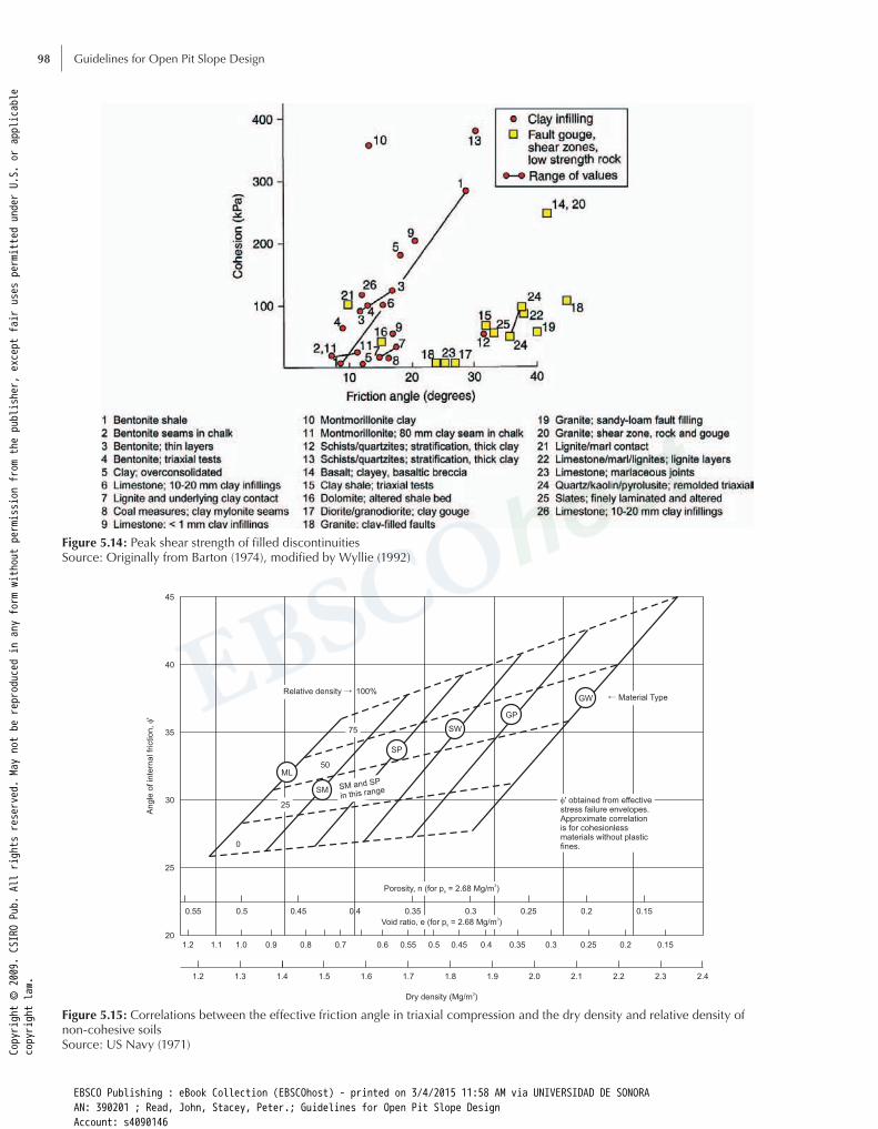
Figure 5.15, prepared by the US Navy (1971), presents correlations between the effective friction angle in triaxial compression and the dry density and relative density of non-cohesive soils as classified by the Unified Soils Classification System (Chapter 2, Table 2.7).
Some of the tests shown in Figure 5.14 also determined residual shear strength values. The tests showed that the residual friction angle was only about 2–4° less than the peak friction angle, while the residual cohesion was essentially zero. Figure 5.16 shows an approximate relationship between the residual friction angle and the plasticity index (PI) of clayey crushed rock (gouge) from a fault. Figure 5.17 shows an empirical correlation between the effective friction angle and the plasticity index of normally consolidated undisturbed clays.
Figure 5.13: Use of triaxial compression test to define the shear strength of veins or other defects with strong infillsSource: Modified from Goodman (1989)
Copyright © 2009. CSI
RO Pub. All rights reserved. May not be reproduced in any form without permission from the publisher, except fair uses permitted under U.S. or applicable
copyright law.
EBSCO Publishing : eBook Collection (EBSCOhost) - printed on 3/4/2015 11:58 AM via UNIVERSIDAD DE SONORAAN: 390201 ; Read, John, Stacey, Peter.; Guidelines for Open Pit Slope DesignAccount: s4090146
Guidelines for Open Pit Slope Design98
Figure 5.14: Peak shear strength of filled discontinuitiesSource: Originally from Barton (1974), modified by Wyllie (1992)
Figure 5.15: Correlations between the effective friction angle in triaxial compression and the dry density and relative density of non-cohesive soilsSource: US Navy (1971)Co
pyright © 2009. CSI
RO Pub. All rights reserved. May not be reproduced in any form without permission from the publisher, except fair uses permitted under U.S. or applicable
copyright law.
EBSCO Publishing : eBook Collection (EBSCOhost) - printed on 3/4/2015 11:58 AM via UNIVERSIDAD DE SONORAAN: 390201 ; Read, John, Stacey, Peter.; Guidelines for Open Pit Slope DesignAccount: s4090146

Rock Mass Model 99
to consider regarding the shear strength of filled discontinuities. In cases where there is a significant decrease in shear strength with displacement, slope failure can occur suddenly following a small amount of movement.
Barton (1974) indicated that filled discontinuities can be divided into two general categories, depending on any previous displacement of the discontinuity. These categories can be further subdivided into normally consolidated (NC) or overconsolidated (OC) materials (Figure 5.18).
Recently displaced discontinuities include faults, sheared zones, clay mylonites and bedding-surface slips. In faults and sheared zones the infilling is formed by the shearing process that may have occurred many times and produced considerable displacement. The crushed material (gouge) formed in this process may include both clay-size particles, and breccia with the particle orientations and striations of the breccia aligned parallel to the direction of shearing. In contrast, the mylonites and bedding-surface slips are defects that were originally clay-bearing and along which sliding occurred during folding or faulting. The shear strength of recently displaced discontinuities will be at, or close to, the residual strength (Graph I in Figure 5.18). Any cohesive bonds that existed in the clay due to previous overconsolidation will have been destroyed by shearing and the infilling will be equivalent to a normally consolidated (NC) material. In addition,
A comparative list of the shear strength values of defects without infills, with thin to medium infills and with thick crushed material from faults (gouge) is provided in Tables 5.8, 5.9 and 5.10.
5.3.2.3 Effect of defect displacement
Wyllie and Norrish (1996) indicated that the shear strength-displacement behaviour is an additional factor
Figure 5.16: Approximate relationship between the residual friction angle (drained tests) and the plasticity index of crushed rock material (gouge) from a faultSource: From Patton & Hendron (1974) and Kanji (1970)
Figure 5.17: Empirical correlation between effective friction angle and plasticity index from triaxial tests on normally consolidated claysSource: Holtz & Kovacs (1981)Copyright © 2009. CSI
RO Pub. All rights reserved. May not be reproduced in any form without permission from the publisher, except fair uses permitted under U.S. or applicable
copyright law.
EBSCO Publishing : eBook Collection (EBSCOhost) - printed on 3/4/2015 11:58 AM via UNIVERSIDAD DE SONORAAN: 390201 ; Read, John, Stacey, Peter.; Guidelines for Open Pit Slope DesignAccount: s4090146

Guidelines for Open Pit Slope Design100
high-strength materials such as quartz and calcite. The infillings of undisplaced discontinuities can be divided into NC and OC materials that have significant differences in peak strength (Graphs II and III in Figure 5.18). While the peak strength of OC clay infillings may be high, there can be a significant loss of strength due to softening, swelling and pore pressure changes on unloading. Strength loss also occurs on displacement in brittle materials such as calcite (Wyllie & Mah 2004).
5.3.2.4 Effect of surface roughnessIn the case of clean rough defects, the roughness increases the friction angle. This was shown by Patton (1966), who
strain-softening may occur with any increase in water content, resulting in a further strength reduction (Wyllie & Mah 2004).
Undisplaced discontinuities that are infilled and have undergone no previous displacement include igneous and metamorphic rocks that have weathered along the discontinuity to form a clay layer. For example, diabase can weather to amphibolite and eventually to clay. Other undisplaced discontinuities include thin beds of clay and weak shales that are found with sandstone in interbedded sedimentary formations. Hydrothermal alteration is another process that forms infillings that can include low-strength materials such as montmorillonite, and
Table 5.8: Shear strength of some structures without infill material
Rock wall/filling material
Shear strength
Comments Reference
Peak Residual
fj
(°)
cj
(kPa)
fjres
(°)
cjres
(kPa)
1: Structures without infills
Crystalline limestone 42–49 0 LT (sn < 4 MPa?) Franklin & Dusseault (1989)
Porous limestone 32–48 0
Chalk 30–41 0
Sandstones 32–37 120–660 24–35 0
Siltstones 20–33 100–790
Soft shales 15–39 0–460
Shales 22–37 0
Schists 32–40 0
Quartzites 23–44 0
Fine-grained igneous rocks 33–52 0
Coarse-grained igneous rocks 31–48 0
Basalt 40–42 0 DST-H (sn < 4 MPa?) Giani (1992)
Calcite 40–42 0
Hard sandstone 34–36 0
Dolomite 30–38 0
Schists 21–36 0
Gypsum 34–35 0
Micaceous quartzite 38–40 0
Gneiss 39–41 0
Copper porphyry 45–60 0 BA of bench failures at Chuquicamata
Granite 45–50 1000–2000 IS (sn < 3 MPa?) Lama & Vutukuri (1978)
Joint in biotitic schist 37–43 0 BA (DA: 120 × 100 m) McMahon (1985)
Joint in quartzite 34–38 0 BA (DA: 20 × 10 m)
LT Laboratory testsDST-H Direct shear tests using a Hoek shear cell or similar BA Back analysis of structurally controlled instabilitiesDA Areal extent of the shear surface considered in the back analysisIS In situ direct shear testsPI Plasticity index of the claySource: Flores & Karzulovic (2003)
Copyright © 2009. CSI
RO Pub. All rights reserved. May not be reproduced in any form without permission from the publisher, except fair uses permitted under U.S. or applicable
copyright law.
EBSCO Publishing : eBook Collection (EBSCOhost) - printed on 3/4/2015 11:58 AM via UNIVERSIDAD DE SONORAAN: 390201 ; Read, John, Stacey, Peter.; Guidelines for Open Pit Slope DesignAccount: s4090146

Rock Mass Model 101
the yielding of the asperities, and cjeq
is the shear strength intercept derived from the asperities which defines a kind of ‘equivalent’ cohesion for the defect (Figure 5.20).
Patton (1966) suggested that asperities can be divided into first- and second-order asperities. First-order asperities are those corresponding to major undulations of the discontinuity. They exhibit wavelengths larger than 0.5 m and roughness angles of not more than about 10–15° (Figure 5.21).
Second-order asperities are those corresponding to small bumps and ripples of the discontinuity with wavelengths smaller than 0.1 m and roughness angles as high as 20–30° (Figure 5.21). Patton (1966) indicated that only first-order asperities have to be considered to obtain reasonable agreement with field observations, but Barton (1973) showed that at low normal stresses second-order asperities also come into play.
studied bedding plane traces in unstable limestone slopes and demonstrated that the rougher the bedding plane the steeper the slope (Figure 5.19).
Based on experimental data for shear of model joints with regular teeth, Patton proposed the following bilinear failure criterion for rough discontinuities:
tan i ifmax n b n ny
#t s f s s= +^ h (eqn 5.28a)
tanc ifmax jeq n jres n ny
$t s f s s= + _ i (eqn 5.28b)
where fb is the basic friction angle of a planar rock
surface, i is the angle of inclination of the failure surface with respect to the direction of the shear force or roughness angle, f
jres is the residual friction angle of the
discontinuity, sny
is the effective normal stress that causes
Table 5.9: Shear strength of some structures with thin to medium thick infill material
Rock wall/filling material
Shear strength
Comments Reference
Peak Residual
fj (°) cj (kPa) fjres (°) cjres (kPa)
2: Structures with thin to medium thickness infills
Bedding plane in layered sandstone and siltstone 12–14 0 BA (DA: 250 ´ 100 m) McMahon (1985)
Bedding plane containing clay in a weathered shale 14–16 0 BA (DA: 30 ´ 30 m)
Bedding plane containing clay in a soft shale 20–24 0 BA (DA: 200 ´ 600m)
Bedding plane containing clay in a soft shale 17–21 0 BA (DA: 120 ´ 180 m)
Bedding plane containing clay in a shale 19–27 0 BA (SD: 80 ´ 60 m)
Foliation plane with chlorite coating in a chloritic schist
33–36 0 BA (DA: 120 ´ 100 m)
Structure in basalt with fillings containing broken rock and clay
42 237 IS (sn: 0–2.5 MPa) Barton (1987)
Shear zone in granite, with brecciated rock and clay gouge
45 254 IS (sn: 0.3-0.7 MPa)
Bedding planes with a clay coating in a quartzite schist
41 725 IS (sn: 0.3-0.9 MPa)
Bedding planes with a clay coating in a quartzite schist
41 598 IS (sn: 0.5-1.1 MPa)
Bedding planes with centimetric clay fillings in a quartzite schist
31 372 IS (sn: 0.2-0.4 MPa)
Limestone joint with clay coatings (<1 mm) 21–17 49–196 IS (sn: 0.1-2.5 MPa)
Limestone joint with millimetric clay fillings 13–14 98
Greywacke bedding plane with clay filling (1–2 mm) 21 0 IS (sn: 0-2.5 MPa)
Clay veins (1–2.5 cm) in coal 16 12 11–12 0 IS (sn < 3 MPa?)
Laminated and altered schists containing clay coatings
33 50
LT Laboratory testsDST-H Direct shear tests using a Hoek shear cell or similar BA Back analysis of structurally controlled instabilitiesDA Areal extent of the shear surface considered in the back analysisIS In situ direct shear testsPI Plasticity index of the claySource: Flores & Karzulovic (2003)
Copyright © 2009. CSI
RO Pub. All rights reserved. May not be reproduced in any form without permission from the publisher, except fair uses permitted under U.S. or applicable
copyright law.
EBSCO Publishing : eBook Collection (EBSCOhost) - printed on 3/4/2015 11:58 AM via UNIVERSIDAD DE SONORAAN: 390201 ; Read, John, Stacey, Peter.; Guidelines for Open Pit Slope DesignAccount: s4090146

Guidelines for Open Pit Slope Design102
that is initially undisturbed and interlocked will have a peak friction angle of (Ø
b + i). With increasing normal
stress and shear displacement, the asperities will be sheared off and the friction angle will progressively diminish to a minimum residual value. This dilation-shearing behaviour is represented by a curved strength envelope with an initial slope equal to tan(Ø
b + i),
reducing to tan(Øjres
) at high normal stresses.
Two other important features of non-planar defects must also be considered.
1 In some cases the surface roughness may display a preferred orientation (eg, undulations, slickensides). In
Wyllie and Norrish (1996) indicated that the actual shear performance of the defects in rock slopes depends on the combined effects of the defect’s roughness and wall rock strength, the applied effective normal stress and the amount of shear displacement. This is illustrated in Figure 5.22, where the asperities are sheared off and there is a consequent reduction in the friction angle with increasing normal stress. In other words, there is a transition from dilation to shearing.
The degree to which the asperities are sheared depends on the magnitude of the effective normal stress in relation to the strength of the asperities and the amount of shear displacement. A rough discontinuity
Table 5.10: Shear strength of crushed material (gouge) from some faults
Rock wall/filling material
Shear strength
Comments Reference
Peak Residual
fj (°) cj (kPa) fjres (°) cjres (kPa)
3: Structures with thick clay gouge fillings (strength defined by gouge material)
Smectites 5–10 0 LT (sn < 4 MPa?) Franklin & Dusseault (1989)Kaolinites 12–15 0
Illites 16–22 0
Chlorites 16–22 0
Clays with IP < 20% 12–28 0 Correlation with the results of laboratory and in situ testing
Hunt (1986)
Clays with 20% < PI < 40% 9–16 0
Clays with 40% < PI < 60% 8–14 0
Clays with IP > 60% 7–12 0
Smooth concrete and clay filling 9–16 240–425 LT (direct shear test) Potyondy (1961)
Bentonite 9–13 60–100 LT (triaxial tests) Barton (1974)
Consolidated clay fillings 12–19 0–180 10–16 0–3
Limestone joint with clay filling (6 cm) 13 0 IS (sn: 0.8-2.5 MPa) Barton (1987)
Shales with clay layers (10–15 cm) 32 78 IS (sn: 0.3-0.8 MPa)
Structures in quartzites and siliceous schists with fillings of brecciated rock and clay gouge (10–15 cm)
32 29 IS (sn: 0.3-1.1 MPa) Barton (1987)
Thick bentonite-montmorillonite vein in chalk (8 cm)
7–8 15 IS (sn < 1 MPa?) Barton (1987)
Fault with clay gouge (5–10 cm) 25 75 BA (planar slide)
4: Structures with thick non-clayey gouge fillings (strength defined by gouge material)
Portland cement grout 16–22 0 LT (sn < 4 MPa?) Franklin & Dusseault (1989)Quartz-feldspar sand 28–40 0
Smooth concrete with compacted silt fillings 40 0 LT (direct shear tests) Potyondy (1961)
Rough concrete with compacted silt fillings 40 0
Smooth concrete with dense sand fillings 44 0
Rough concrete with dense sand fillings 44 0
LT Laboratory testsDST-H Direct shear tests using a Hoek shear cell or similar BA Back analysis of structurally controlled instabilitiesDA Areal extent of the shear surface considered in the back analysisIS In situ direct shear testsPI Plasticity index of the claySource: Flores & Karzulovic (2003)
Copyright © 2009. CSI
RO Pub. All rights reserved. May not be reproduced in any form without permission from the publisher, except fair uses permitted under U.S. or applicable
copyright law.
EBSCO Publishing : eBook Collection (EBSCOhost) - printed on 3/4/2015 11:58 AM via UNIVERSIDAD DE SONORAAN: 390201 ; Read, John, Stacey, Peter.; Guidelines for Open Pit Slope DesignAccount: s4090146

Rock Mass Model 103
is. This is discussed in detail by Goodman (1989), who showed that the shear strength of non-planar defects depends on the stress path, due to the interaction between the normal and tangential deformations, the dilatancy and the normal and shear stresses. This is usually ignored in practice. Usually, the shear strength criteria assume that the normal stress remains constant
these cases, the shear strength of the defect will be affected by the direction of sliding, where the shear strength is much greater across the corrugations than along them (Figure 5.23). This effect can be very important in slope stability analyses.
2 The shear strength is affected by how the normal load is applied and how restricted the dilatancy of the defect
Figure 5.18: Simplified classification of filled defects into displaced and undisplaced, and normally consolidated (NC) and overconsolidated (OC) types of infill materialSource: Modified from Barton (1974) by Wyllie & Norrish (1996)
Figure 5.19: Patton’s observation of bedding plane traces in unstable limestone slopesSource: Patton (1966)
b
jres
cjeq
i
ny
b
f
f
jres
cjeq
i
ssny
t
Figure 5.20: Patton’s bilinear failure criterion for the shear strength of rough defects
Copyright © 2009. CSI
RO Pub. All rights reserved. May not be reproduced in any form without permission from the publisher, except fair uses permitted under U.S. or applicable
copyright law.
EBSCO Publishing : eBook Collection (EBSCOhost) - printed on 3/4/2015 11:58 AM via UNIVERSIDAD DE SONORAAN: 390201 ; Read, John, Stacey, Peter.; Guidelines for Open Pit Slope DesignAccount: s4090146

Guidelines for Open Pit Slope Design104
tanJ
Jj
a
r1.f - e o (eqn 5.29)
where Jr is the joint roughness and J
a is the joint alteration
number. Peak friction angle values obtained using this approach are given in Table 5.11 and should be compared with the values for defects either without infill material or with thin to medium thicknesses of infill material given in Tables 5.8 and 5.9.
5.3.2.5 Barton-Bandis failure criterion
Barton (1971, 1973) used the concepts of joint roughness and wall strength to introduce the non-linear empirical Barton-Bandis criterion for the shear strength of the defects in a rock mass. The criterion defines the peak shear strength of a discontinuity as:
tan logJRCJCS
max nn
b10t s s f= +dd n n (eqn 5.30)
where fb is the basic friction angle, JRC is the joint
roughness coefficient and JCS is the uniaxial compressive strength of the rock wall.
during the shearing process even if the structure is rough. This may be permissible for open pit slopes, where a sliding block does not impose major restrictions on dilatancy. It is not necessarily permissible for an underground mine where there may be heavy restrictions on dilatancy, especially if two of the faces of a potentially instable block are parallel or quasi-parallel.
As a means of taking joint roughness and the wall rock strength into account, Barton and Bandis (1981) suggested that a first estimate of the peak friction angle can be obtained by assuming that:
Figure 5.21: Definition of first- and second-order asperities on rough defectsSource: Wyllie & Norrish (1996)
Figure 5.22: Effect of surface roughness and normal stress on the defect’s friction angleSource: Wyllie (1992)
Figure 5.23: Roughness-induced shear strength anisotropySource: Simons et al. (2001)
Copyright © 2009. CSI
RO Pub. All rights reserved. May not be reproduced in any form without permission from the publisher, except fair uses permitted under U.S. or applicable
copyright law.
EBSCO Publishing : eBook Collection (EBSCOhost) - printed on 3/4/2015 11:58 AM via UNIVERSIDAD DE SONORAAN: 390201 ; Read, John, Stacey, Peter.; Guidelines for Open Pit Slope DesignAccount: s4090146

Rock Mass Model 105
the ratio (JCS/sn). Hence, equation (5.3) can be
rewritten as:
tan tan imax n j n bt s f s f= = +_ ^i h (eqn 5.31)
where the friction angle of the defect, fj, is represented by
the basic friction angle, fb, plus an increment i that
depends on the roughness of the discontinuity and the magnitude of the effective normal stress relative to the uniaxial compressive strength of the wall rock. This increment is given by:
logi JRCJCS
n10 s= d n (eqn 5.32)
The values of roughness and i reach their maximum at low values of s
n. As s
n increases, some of the asperities will
yield and the effect of roughness will decrease. As sn
moves towards the value of JCS, more asperities yield and the effect of roughness diminishes. Eventually, all the asperities yield and the effect of roughness is totally overcome. When this occurs, f
j equals f
b.
Usually fb takes values of the order of 30°. The values
given in Table 5.12 give a guide for first estimates for
As originally formulated by Barton (1973), the criterion applies only to defects of geological origin, meaning defects that were formed as a consequence of brittle failure. Defects that were subsequently modified by processes such as (a) the passage of mineralising solutions, which left behind a variety of infillings ranging from soft to weak to hard and strong such as clay, talc, gypsum, pyrite and quartz on the defect faces or (b) tectonic events, for example faulting and plastic deformation such as foliation, slaty cleavage and gniessosity, were excluded. The exclusion of all filled defects means that weathering and alteration can only be considered if the rock walls of the defect are still in direct rock/rock contact. The net effect of this exclusion means that the Barton-Bandis criterion cannot be applied to many of the geological environments found in pit slope engineering. Consequently, the criterion must be applied with great caution.
Notwithstanding these limitations, the advantage of the Barton-Bandis criterion is that it includes explicitly the effects of surface roughness, through the parameter JRC, and of the magnitude of the normal stress through
Table 5.11: First estimates of the peak friction angle of defects obtained from the joint roughness number, Jr, and the joint alteration number, Ja
Joint alteration number, Ja
Tightly healed,
hard, non-
softening,
impermeable
filling, e.g.
quartz or
epidote
Unaltered
joint walls,
surface
staining only
Slightly altered
joint walls,
non-softening
mineral
coatings,
sandy
particles,
clay-free
disintegrated
rock etc.
Silty- or
sandy-clay
coatings,
small clay
fraction
(non-
softening)
Softening or
low-friction clay
mineral
coatings, i.e.
kaolinite or
mica. Also
chlorite, talc,
gypsum,
graphite etc.
and small
quantities of
swelling clays
A B C D E
Joint roughness number, Jr Ja
Description Jr 0.75 1 2 3 4
A Discontinuous joints 4 70° 60° 55° 45°
B Rough, undulating joints 3 70° 55° 45° 35°
C Smooth, undulating joints 2 65° 60° 45° 35° 25°
D Slickensided, undulating joints 1.5 60° 55° 35° 25° 20°
E Rough or irregular, planar joints 1.5 60° 55° 35° 25° 20°
F Smooth, planar joints 1.0 50° 45° 25° 18° 15°
G Slickensided, planar joints 0.5 35° 25° 15° <10°
NotesThe joint roughness number assumes rock wall contact or rock wall contact before 10 cm of shear displacement.The descriptions of different cases for Jr refer to small-scale features and intermediate-scale features, in that order.The joint alteration number assumes rock wall contact.These are first estimates of peak friction angle and may not be appropriate for site-specific design purposes.
Copyright © 2009. CSI
RO Pub. All rights reserved. May not be reproduced in any form without permission from the publisher, except fair uses permitted under U.S. or applicable
copyright law.
EBSCO Publishing : eBook Collection (EBSCOhost) - printed on 3/4/2015 11:58 AM via UNIVERSIDAD DE SONORAAN: 390201 ; Read, John, Stacey, Peter.; Guidelines for Open Pit Slope DesignAccount: s4090146

Guidelines for Open Pit Slope Design106
some rock types. In practice, fb can be determined from
simple tilt-table tests or from direct shear tests on saw-cut rock samples.
The joint roughness coefficient, JRC, varies from 0° for smooth, planar and slickensided surfaces to as much as 20° for rough undulating surfaces. There are a number of different ways of evaluating JRC, but the procedure most widely used is to visually compare the surface condition with standard profiles based on a combination of surface irregularities and waviness using profiles such as those shown in Tables 5.13 and 5.14, or the chart shown in Table 5.15. Tables 5.13 and 5.14 are widely used in practice, but require judgment regarding the scale effects of JRC.
Less usual methods include measuring roughness using a mechanical profilometer or carpenter’s comb (Tse & Cruden 1979) or conducting tilt and/or pullout tests on rock blocks (Barton & Bandis 1981).
The value of JCS may be assumed to be similar to the uniaxial compressive strength of rock, s
c, if the defect
rock walls are sound and not altered. If the rock walls are highly weathered and/or altered, the value of JCS may be smaller than 0.25s
c. The Schmidt hammer can be
used to evaluate JCS using charts like the one shown in Table 5.16, or the correlation proposed by Deere and Miller (1966):
.JCS 6 9 10 . .R L0 0087 0 16n#= r +]^ g h (eqn 5.33)
where JCS is in MPa units, r is the rock density in g/cm3 units and R
n(L) is the rebound number of the L-type
Schmidt hammer. Caution is suggested when using this correlation due to the large dispersion of values commonly found. There are several correlations between the uniaxial compressive strength of rock and the Schmidt hammer rebound number (see Zhang 2005). Alternatively, the ISRM empirical field estimates of s
c shown in Table 2.3
can be used.
5.3.2.6 Scale effectsAlthough discussions about the effects of scale on the shear strength of defects as defined by the Mohr-Coulomb
failure criterion (cj and f
j) are limited, the available data
indicates that:
■ laboratory tests frequently overestimate the shear strength of discontinuities, especially the cohesion;
■ the results of several back analyses of structurally controlled instabilities indicate that the peak shear strength of clean structures with sound hard rock walls, at scales from 10–30 m and in a low confine-
Table 5.12: Typical values of the basic friction angle, fb, for some rock types
Rock type fb dry fb wet Rock type fb dry fb wet
Amphibolite 32° Granite, fine-grained 31–35° 29–31°
Basalt 35–38° 31–36° Granite, coarse-grained 31–35° 31–33°
Chalk 30° Limestone 31–37° 27–35°
Conglomerate 35° Sandstone 26–35° 25–34°
Copper porphyry 31° Schist 27°
Dolomite 31–37° 27–35° Siltstone 31–33° 27–31°
Gneiss, schistose 26–29° 23–26° Slate 25–30° 21°
Source: Data from Barton (1973), Barton & Choubrey (1977)
Table 5.13: Defect roughness profiles and associated JRC values
Source: Modified from Barton & Choubray (1977)
Copyright © 2009. CSI
RO Pub. All rights reserved. May not be reproduced in any form without permission from the publisher, except fair uses permitted under U.S. or applicable
copyright law.
EBSCO Publishing : eBook Collection (EBSCOhost) - printed on 3/4/2015 11:58 AM via UNIVERSIDAD DE SONORAAN: 390201 ; Read, John, Stacey, Peter.; Guidelines for Open Pit Slope DesignAccount: s4090146

Rock Mass Model 107
Table 5.14: ISRM-suggested characterisation of defect roughness
Class
Scale
Typical roughness profile JRC20 JRC100Intermediate Minor
I Stepped Rough 20 11
II Smooth 14 9
III Slickensided 11 8
IV Undulating Rough 14 9
V Smooth 11 8
VI Slickensided 7 6
VII Planar Rough 2.5 2.3
VIII Smooth 1.5 0.9
IX Slickensided 0.5 0.4
NotesThe length of the roughness profiles is intended to be in the range of 1–10 cmThe vertical and horizontal scales are identicalJRC20 and JRC100 correspond to joint roughness coefficient when the roughness profiles are ‘scaled’ to a length of 20 cm and 100 cm respectivelySource: Modified from Brown (1981) and Barton & Bandis (1990) by Flores & Karzulovic (2003)
Table 5.15: Estimating JRC from the maximum unevenness amplitude and the profile length
0.1 0.2 0.3 0.5 0.8 1 2 3 5 8 10
Profile Length (m)
Un
even
ess
Am
plit
ude
(mm
)
1
PROFILE LENGTH (m)
1
UNEVENESS AMPLITUDE (mm)
PROFILE LENGTH (m)
400
300
200
10080
50
30
20
108
5
3
2
10.8
0.5
0.3
0.2
0.1
2016121086543
2
1
0.5
Join
t Ro
ugh
ness C
oefficien
t, JRC
Source: Barton (1982)
Table 5.16: Estimating the uniaxial compressive strength, sc, of the defect rock wall from Schmidt hardness values
Source: Hoek (2002)
Copyright © 2009. CSI
RO Pub. All rights reserved. May not be reproduced in any form without permission from the publisher, except fair uses permitted under U.S. or applicable
copyright law.
EBSCO Publishing : eBook Collection (EBSCOhost) - printed on 3/4/2015 11:58 AM via UNIVERSIDAD DE SONORAAN: 390201 ; Read, John, Stacey, Peter.; Guidelines for Open Pit Slope DesignAccount: s4090146
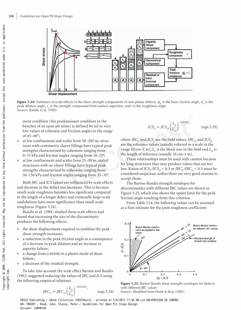
Guidelines for Open Pit Slope Design108
ment condition (the predominant condition in the benches of an open pit mine) is defined by nil to very low values of cohesion and friction angles in the range of 45–60°;
■ at low confinement and scales from 50–200 m, struc-tures with centimetric clayey fillings have typical peak strengths characterised by cohesions ranging from 0–75 kPa and friction angles ranging from 18–25°;
■ at low confinement and scales from 25–50 m, sealed structures with no clayey fillings have typical peak strengths characterised by cohesions ranging from 50–150 kPa and friction angles ranging from 25–35°.
Both JRC and JCS values are influenced by scale effects and decrease as the defect size increases. This is because small-scale roughness becomes less significant compared to the length of a longer defect and eventually large-scale undulations have more significance than small-scale roughness (Figure 5.24).
Bandis et al. (1981) studied these scale effects and found that increasing the size of the discontinuity produces the following effects:
■ the shear displacement required to mobilise the peak shear strength increases;
■ a reduction in the peak friction angle as a consequence of a decrease in peak dilation and an increase in asperity failure;
■ a change from a brittle to a plastic mode of shear failure;
■ a decrease of the residual strength.
To take into account the scale effect Barton and Bandis (1982) suggested reducing the values of JRC and JCS using the following empirical relations:
JRC JRCL
L . /
F OO
FJRC0 02
O
=
-
e o (eqn 5.34)
JCS JCSL
L .
F OO
FJRC0 03
O
=
-
e o (eqn 5.35)
where JRCF and JCS
F are the field values, JRC
O and JCS
O
are the reference values (usually referred to a scale in the range 10 cm–1 m), L
F is the block size in the field and L
O is
the length of reference (usually 10 cm–1 m).These relationships must be used with caution because
for long structures they may produce values that are too low. Ratios of JCS
F /JCS
O < 0.3 or JRC
F /JRC
O < 0.5 must be
considered suspicious unless there are very good reasons to accept them.
The Barton-Bandis strength envelopes for discontinuities with different JRC values are shown in Figure 5.25, which also shows the upper limit for the peak friction angle resulting from this criterion.
From Table 5.14, the following values can be assumed as a first estimate for the joint roughness coefficient:
Figure 5.24: Summary of scale effects in the shear strength components of non-planar defects. fb is the basic friction angle, dn is the peak dilation angle, sa is the strength component from surface asperities, and i is the roughness angleSource: Bandis et al. (1981)
Figure 5.25: Barton-Bandis shear strength envelopes for defects with different JRC valuesSource: Modified from Hoek & Bray (1981)
Copyright © 2009. CSI
RO Pub. All rights reserved. May not be reproduced in any form without permission from the publisher, except fair uses permitted under U.S. or applicable
copyright law.
EBSCO Publishing : eBook Collection (EBSCOhost) - printed on 3/4/2015 11:58 AM via UNIVERSIDAD DE SONORAAN: 390201 ; Read, John, Stacey, Peter.; Guidelines for Open Pit Slope DesignAccount: s4090146

Rock Mass Model 109
■ rough undulating discontinuities: JRC ≈ 15–20 ■ smooth undulating discontinuities: JRC ≈ 10 ■ smooth planar discontinuities: JRC ≈ 2
5.3.2.7 Stress, strain and normal stiffness
Numerical slope stability analyses require, in addition to the strength properties, the stress-strain characteristics of defects. Detailed discussions on the stress-strain behaviour of defects can be found in Goodman (1976), Bandis et al. (1983), Barton (1986), Bandis (1993) and Priest (1993).
The loading of a discontinuity induces normal and shear displacements whose magnitude depends on the stiffness of the structure, defined in terms of a normal stiffness, k
n, and a shear stiffness, k
s. These refer to the rate
of change of normal (sn) and shear (t) stresses with
respect to normal (vc) and shear (u
s) displacements
(Bandis 1993):
dd
kk
dvdu0
0n n
s
c
s
st =
= G' )1 3 (eqn 5.36)
where:
kvn
c
n
us2
2s= f p (eqn 5.37a)
kus
s vc22t
= d n (eqn 5.37b)
Therefore, a discontinuity subjected to normal and shear stresses will suffer normal and shear displacements that depend on the following factors:
■ the initial geometry of the discontinuity’s rock walls; ■ the matching between the rock walls, which defines the
variation of the aperture and the effective contact area (Figure 5.26);
■ the strength and deformability of the rock wall material;
■ the thickness and mechanical properties of the filling material (if any);
■ the initial values of the normal and shear stresses acting on the structure.
It is assumed that the defect cannot sustain tensile normal stresses and that there will be a limiting compressive normal stress beyond which the defect is mechanically indistinguishable from the surrounding rock (Figure 5.27).
Figure 5.26: Examples of discontinuities with matching and mismatching rock wallsSource: Flores & Karzulovic (2003)
Figure 5.27: Determination of the normal stiffness of an artificial defect by means of uniaxial compression tests on specimens of granodiorite with and without a discontinuity. (a) Normal stress-total axial displacement curves. (b) Normal stress-discontinuity closure curvesSource: Goodman (1976)
Copyright © 2009. CSI
RO Pub. All rights reserved. May not be reproduced in any form without permission from the publisher, except fair uses permitted under U.S. or applicable
copyright law.
EBSCO Publishing : eBook Collection (EBSCOhost) - printed on 3/4/2015 11:58 AM via UNIVERSIDAD DE SONORAAN: 390201 ; Read, John, Stacey, Peter.; Guidelines for Open Pit Slope DesignAccount: s4090146

Guidelines for Open Pit Slope Design110
The normal stiffness of a defect can be measured from a compression test with the load perpendicular to the discontinuity (Goodman 1976), or from a direct shear test if normal displacements are measured for different normal stresses (Figure 5.12). The following comments can be made.
1 Normal stiffness depends on the rock wall properties and geometry, the matching between rock walls, the filling thickness and properties (if any), the initial condition (before applying a normal stress increment), the magnitude of the normal stress increment and the number of loading cycles.
2 Generally, normal stiffness is larger if the rock wall and filling material (if any) are stronger and stiffer.
3 For a given set of conditions, normal stiffness is larger for defects with good matching than for mismatching ones.
4 Normal stiffness increases with the number of loading cycles. Apparently, the increment is larger in the case of stronger and stiffer rock walls.
5 The values quoted in the geotechnical literature indicate that normal stiffness ranges from 0.001–2000 GPa/m. It typically takes the following values:
→ defects with soft infills: kn < 10 GPa/m;
→ clean defects in moderately strong rock: kn =
10–50 GPa/m; → clean defects in strong rock: k
n = 50–200 GPa/m.
The normal stiffness of a defect increases as the defect closes when s
n increases, but there is a limit that is reached
when the defect reaches its maximum closure, vcmax
. Assuming that the relationship between the effective normal stress, s
n, and the defect closure, v
c, is hyperbolic
(Goodman et al. 1968) it is possible to define the normal stiffness (Zhang 2005):
k kk v
1max
n nini c
n2s
= +f p (eqn 5.38)
where kni
is the initial normal stiffness, defined as the initial tangent of the normal stress-discontinuity closure curve (Figure 5.29). As the defect’s tensile strength is usually neglected, k
n = 0 if s
n is tensile.
Hence, to determine the normal stiffness of a defect it is necessary to know the initial value of this stiffness and the defect’s maximum closure. From experimental results, Bandis et al. (1983) suggested that k
ni for matching defects
can be evaluated as:
. . .k JRC eJCS
7 15 1 75 0 02ni
i.- + + d n (eqn 5.39)
where kni
is in GPa/m units (or MPa/mm), JRC and JCS are coefficients of the Barton-Bandis failure criterion and e
i is
the initial aperture of the discontinuity, which can be estimated as:
.
.e JRCJCS
0 040 02
i
c.
s-d n (eqn 5.40)
where ei is in mm, and s
c and JCS are in MPa.
For the case of mismatching structures, Bandis et al. (1983) suggested the following relationship:
. .
kJRC JCS
k
2 0 0 0004,ni mmn
ni
# # # s=+
(eqn 5.41)
where kni,mm
is the initial tangent stiffness for mismatching defects. Regarding the scale effect on the normal stiffness, it can be implicitly considered by using ‘scaled’ values for JRC and JCS, and an ‘adequate’ value for e
i. Although these
relationships have several limitations there are few practical tools to estimate k
n. Some reported values for the
normal stiffness of discontinuities are listed in Tables 5.17 and 5.18.
Figure 5.28: Definition of kn and kni in an effective normal stress-discontinuity closure curve
Shear displacement, us
sn
Sh
ea
r str
ess, t
us,peak
max
1us
ks,peak
Shear displacement, us
nn
t
Sh
ea
r str
ess,
us,peak
tmax
1us
ks,peak
Figure 5.29: Determination of secant peak shear stiffness of a defect from a direct shear stressSource: Goodman (1970)
Copyright © 2009. CSI
RO Pub. All rights reserved. May not be reproduced in any form without permission from the publisher, except fair uses permitted under U.S. or applicable
copyright law.
EBSCO Publishing : eBook Collection (EBSCOhost) - printed on 3/4/2015 11:58 AM via UNIVERSIDAD DE SONORAAN: 390201 ; Read, John, Stacey, Peter.; Guidelines for Open Pit Slope DesignAccount: s4090146

Rock Mass Model 111
Table 5.17: Reported values for normal stiffness for some rocks
Rock Discontinuity
Load
cycle
kni
(GPa/m)
kN
(GPa/m) Comments Reference
SA
ND
STO
NE
Fresh to slightly weathered,good matching of rock walls
1 4–23 sni = 1 kPa Bandis et al. (1983)2 11–35
3 18–62Moderately weathered,good matching of rock walls
1 4–262 9–273 15–45
Weathered,good matching of rock walls
1 2–52 9–143 11–20
Shear zone with clay gouge 1.7 Estimated from data in reference, assuming a 3 cm thickness
Wittke (1990)
Bedding planes, good matching(JRC = 10–16)
13–24 Direct shear tests with sn ranging from 0.4–0.9 MPa
Rode et al. (1990)
Bedding planes, good matching(JRC = 10–16)
7–12
Fresh fractures, good matching(JRC = 12–17)
17–25
Fresh fractures, poor matching(JRC = 12–17)
8–12
LIM
ES
TON
E
Fresh to slightly weathered,good matching
1 8–31 sni = 1 kPa Bandis et al. (1983)2 54–134
3 72–160Moderately weathered,good matching
1 5–702 26–913 53–168
Weathered, good matching 1 4–132 40–503 42–65
Joints in weathered limestone 0.5–1.0 sn = 5 MPa Bandis (1993)Joints in fresh limestone 4–5
QU
AR
TZIT
E Clean 15–30 sn = 10–20 MPa Ludvig (1980)With clay gouge 10–25
DO
LER
ITE
Fresh, good matching 1 21–27 sni = 1 kPa Bandis et al. (1983)2 59–75
3 103–119Weathered, good matching 1 8–13
2 24–923 37–130
GR
AN
ITE
Clean joint (JRC = 1.9) 1 121 Estimated from ref.Biaxial testssn : 25–30 MPa
Makurat et al. (1990)Clean joint (JRC = 3.8) 1 74
Clean joint 352–635 Mes. Sist. Pac-ex.sn: 8.6–9.3 MPa
Martín et al. (1990)50–110
Shear zone 2–224 Mes. Sist. Pac-ex.sn: 0.5–1.5 MPa
7–266 Mes. Sist. Pac-ex.sn : 18–20 MPa
kn = Normal stiffnesssn = Normal stresskni = Initial normal stiffnesssni = Initial normal stressPac-ex: Measured by the system Pac-ex, a special instrumentation system developed in the Underground Research Laboratory by Atomic Energy of Canada Ltd.Source: Flores & Karzulovic (2003)
Copyright © 2009. CSI
RO Pub. All rights reserved. May not be reproduced in any form without permission from the publisher, except fair uses permitted under U.S. or applicable
copyright law.
EBSCO Publishing : eBook Collection (EBSCOhost) - printed on 3/4/2015 11:58 AM via UNIVERSIDAD DE SONORAAN: 390201 ; Read, John, Stacey, Peter.; Guidelines for Open Pit Slope DesignAccount: s4090146

Guidelines for Open Pit Slope Design112
Table 5.18: Reported values for normal stiffness for some rocks
Rock Discontinuity
Load
cycle
kni
(GPa/m)
kN
(GPa/m) Comments Reference
SIL
TSTO
NE
Fresh, good matching 1 14–26 sni = 1 kPa Bandis et al. (1983)
2 22–64
3 22–70
Moderately weathered, good matching
1 10–11
2 20–22
3 20–26
Weathered, good matching 1 7–14
2 27–29
3 29–41
QU
AR
TZ
MO
NZO
NIT
E Clean 15.3 Triaxial testing (?) Goodman & Dubois (1972)
PL
AS
TER Clean, artificial fractures 2.7–5.4 sn: 3.5–24 MPa Barton (1972)
Clean, artificial fractures 2.7 Karzulovic (1988)
SL
ATE
Fresh, good matching 1 24–47 sni = 1 kPa Bandis et al. (1983)
2 98–344
3 185–424
Weathered 1 11–14
2 19–40
3 49–78
RH
YOLI
TE Clean 16.4 Triaxial testing (?) Goodman & Dubois (1972)
WE
AK
R
OC
K With clay gouge 5–40 Increases with sn Barton et al. (1981)
HA
RD
RO
CK
Soft clay filling 0.01–0.1 Typical range Itasca (2004)
Clean 37–93 Triaxial testing. Increases with number of loading cycles
Rosso (1976)
8–99 Direct shear tests
Clean fracture 1620 Estimate for numerical analysis
Rutqvist et al. (1990)
Good match, interlocked > 100 Typical value Itasca (2004)
Fault with clay gouge 0.005 30–150 cm thick Karzulovic (1988)
Rough structure with a fill of rock powder
0.8 Mismatching
GY
PS
UM
Fresh joints (JRC = 11) 1 3–11 sni = 0.2 MPa Rode et al. (1990)
Fresh joints (JRC = 11) > 1 10–13
kn = Normal stiffnesssn = Normal stresskni = Initial normal stiffnesssni = Initial normal stressPac-ex: Measured by the system Pac-ex, a special instrumentation system developed in the Underground Research Laboratory by Atomic Energy of Canada Ltd.Source: Flores & Karzulovic (2003)
Copyright © 2009. CSI
RO Pub. All rights reserved. May not be reproduced in any form without permission from the publisher, except fair uses permitted under U.S. or applicable
copyright law.
EBSCO Publishing : eBook Collection (EBSCOhost) - printed on 3/4/2015 11:58 AM via UNIVERSIDAD DE SONORAAN: 390201 ; Read, John, Stacey, Peter.; Guidelines for Open Pit Slope DesignAccount: s4090146
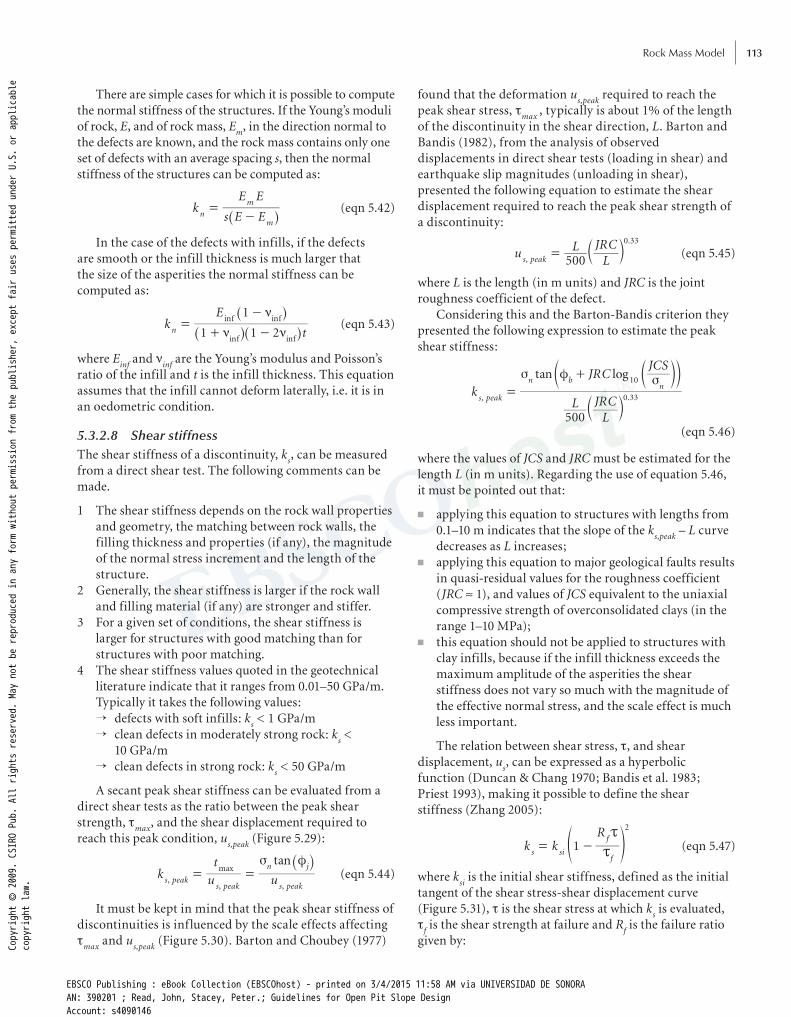
Rock Mass Model 113
There are simple cases for which it is possible to compute the normal stiffness of the structures. If the Young’s moduli of rock, E, and of rock mass, E
m, in the direction normal to
the defects are known, and the rock mass contains only one set of defects with an average spacing s, then the normal stiffness of the structures can be computed as:
ks E E
E En
m
m=
-^ h (eqn 5.42)
In the case of the defects with infills, if the defects are smooth or the infill thickness is much larger that the size of the asperities the normal stiffness can be computed as:
kt
E
1 1 2
1
inf inf
inf inf
n n nn
=+ -
-
^ ^^h h
h (eqn 5.43)
where Einf
and ninf
are the Young’s modulus and Poisson’s ratio of the infill and t is the infill thickness. This equation assumes that the infill cannot deform laterally, i.e. it is in an oedometric condition.
5.3.2.8 Shear stiffnessThe shear stiffness of a discontinuity, k
s, can be measured
from a direct shear test. The following comments can be made.
1 The shear stiffness depends on the rock wall properties and geometry, the matching between rock walls, the filling thickness and properties (if any), the magnitude of the normal stress increment and the length of the structure.
2 Generally, the shear stiffness is larger if the rock wall and filling material (if any) are stronger and stiffer.
3 For a given set of conditions, the shear stiffness is larger for structures with good matching than for structures with poor matching.
4 The shear stiffness values quoted in the geotechnical literature indicate that it ranges from 0.01–50 GPa/m. Typically it takes the following values:
→ defects with soft infills: ks < 1 GPa/m
→ clean defects in moderately strong rock: ks <
10 GPa/m → clean defects in strong rock: k
s < 50 GPa/m
A secant peak shear stiffness can be evaluated from a direct shear tests as the ratio between the peak shear strength, t
max, and the shear displacement required to
reach this peak condition, us,peak
(Figure 5.29):
tan
k u
t
u,, ,
max
s peaks peak s peak
n js f
= =_ i
(eqn 5.44)
It must be kept in mind that the peak shear stiffness of discontinuities is influenced by the scale effects affecting t
max and u
s,peak (Figure 5.30). Barton and Choubey (1977)
found that the deformation us,peak
required to reach the peak shear stress, t
max , typically is about 1% of the length
of the discontinuity in the shear direction, L. Barton and Bandis (1982), from the analysis of observed displacements in direct shear tests (loading in shear) and earthquake slip magnitudes (unloading in shear), presented the following equation to estimate the shear displacement required to reach the peak shear strength of a discontinuity:
u LL
JRC500,
.
s peak
0 33
= c m (eqn 5.45)
where L is the length (in m units) and JRC is the joint roughness coefficient of the defect.
Considering this and the Barton-Bandis criterion they presented the following expression to estimate the peak shear stiffness:
tan log
kL
LJRC
JRCJCS
500
, .s peak
n bn
10
0 33
s f s=
+
c
dd
m
nn
(eqn 5.46)
where the values of JCS and JRC must be estimated for the length L (in m units). Regarding the use of equation 5.46, it must be pointed out that:
■ applying this equation to structures with lengths from 0.1–10 m indicates that the slope of the k
s,peak – L curve
decreases as L increases; ■ applying this equation to major geological faults results
in quasi-residual values for the roughness coefficient (JRC ≈ 1), and values of JCS equivalent to the uniaxial compressive strength of overconsolidated clays (in the range 1–10 MPa);
■ this equation should not be applied to structures with clay infills, because if the infill thickness exceeds the maximum amplitude of the asperities the shear stiffness does not vary so much with the magnitude of the effective normal stress, and the scale effect is much less important.
The relation between shear stress, t, and shear displacement, u
s, can be expressed as a hyperbolic
function (Duncan & Chang 1970; Bandis et al. 1983; Priest 1993), making it possible to define the shear stiffness (Zhang 2005):
k kR
1s si
f
f2
x
x= -f p (eqn 5.47)
where ksi is the initial shear stiffness, defined as the initial
tangent of the shear stress-shear displacement curve (Figure 5.31), t is the shear stress at which k
s is evaluated,
tf is the shear strength at failure and R
f is the failure ratio
given by:Copyright © 2009. CSI
RO Pub. All rights reserved. May not be reproduced in any form without permission from the publisher, except fair uses permitted under U.S. or applicable
copyright law.
EBSCO Publishing : eBook Collection (EBSCOhost) - printed on 3/4/2015 11:58 AM via UNIVERSIDAD DE SONORAAN: 390201 ; Read, John, Stacey, Peter.; Guidelines for Open Pit Slope DesignAccount: s4090146
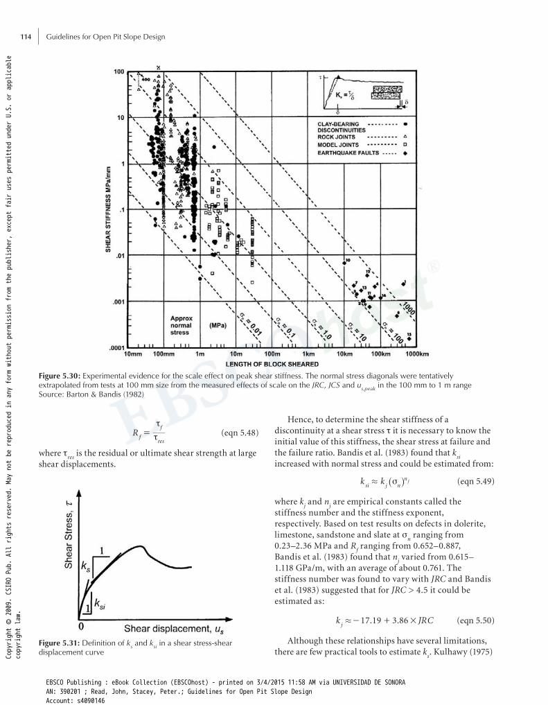
Guidelines for Open Pit Slope Design114
Rf
res
f
tt
= (eqn 5.48)
where tres
is the residual or ultimate shear strength at large shear displacements.
Hence, to determine the shear stiffness of a discontinuity at a shear stress t it is necessary to know the initial value of this stiffness, the shear stress at failure and the failure ratio. Bandis et al. (1983) found that k
si
increased with normal stress and could be estimated from:
k ksi j n
n j. s^ h (eqn 5.49)
where kj and n
j are empirical constants called the
stiffness number and the stiffness exponent, respectively. Based on test results on defects in dolerite, limestone, sandstone and slate at s
n ranging from
0.23–2.36 MPa and Rf ranging from 0.652–0.887,
Bandis et al. (1983) found that nj varied from 0.615–
1.118 GPa/m, with an average of about 0.761. The stiffness number was found to vary with JRC and Bandis et al. (1983) suggested that for JRC > 4.5 it could be estimated as:
. .k JRC17 19 3 86j
#.- + (eqn 5.50)
Although these relationships have several limitations, there are few practical tools to estimate k
s. Kulhawy (1975)
Figure 5.30: Experimental evidence for the scale effect on peak shear stiffness. The normal stress diagonals were tentatively extrapolated from tests at 100 mm size from the measured effects of scale on the JRC, JCS and us,peak in the 100 mm to 1 m rangeSource: Barton & Bandis (1982)
Figure 5.31: Definition of ks and ksi in a shear stress-shear displacement curveCo
pyright © 2009. CSI
RO Pub. All rights reserved. May not be reproduced in any form without permission from the publisher, except fair uses permitted under U.S. or applicable
copyright law.
EBSCO Publishing : eBook Collection (EBSCOhost) - printed on 3/4/2015 11:58 AM via UNIVERSIDAD DE SONORAAN: 390201 ; Read, John, Stacey, Peter.; Guidelines for Open Pit Slope DesignAccount: s4090146

Rock Mass Model 115
There are some simple cases for which it is possible to compute the shear stiffness of the structures. If the shear moduli of rock, G, and of rock mass, G
m, are known for
shear in the direction parallel to the defects, and the rock mass contains only one set of discontinuities with an
presented data on shear stiffness of defects evaluated both at the peak and yield points of the shear stress-shear displacement curves, k
s,peak and k
s,yield. Some reported
values for the shear stiffness of discontinuities are listed in Tables 5.19 and 5.20.
Table 5.19: Reported values for shear stiffness of some defects
Rock Structure type
ksi
(GPa/m)
ks,yield
(GPa/m)
ks,peak
(GPa/m) Comments Reference
AMPHIBOLITE Schistosity plane 0.59 DST, sni = 0.12 MPa Kulhawy (1975)SANDSTONE Sandstone-basalt contact 0.11 DST, sni = 0.13 MPa
Sandstone-chalk contact 0.3–2.1 0.1–0.2 DST, sni = 0.1–1 MPa
Artificial fracture 29.8 DST, sni = 0.26 MPa
Artificial rough fracture 1.3 DST, sni = 2.4 MPa
Artificial clean fracture 5–38 Maki (1985)
Fresh fracture, good matching 2.2–38 0.6–4.5 sn = 0.2–2.4 MPa Bandis et al. (1983)Slightly weathered fracture, good
matching9–42 1.2–4.7 sn = 0.2-2.1 MPa
Moderately weathered fracture, good matching
1.2–6 0.5–1.7 sn = 0.2–2.0 MPa
Weathered fracture, good matching 2.1–7 0.6–1.4 sn = 0.5–2.0 MPa
LIMESTONE Clean smooth fractures 0.4–2.4 0.2–1.3 DST, sni = 0.9–2.4 MPa Kulhawy (1975)Artificial fracture 8.7 DST, sni = 10.4 MPa
Clean artificial fracture 3–17 Maki (1985)
Fresh to slightly weathered, good matching
8–51 1.7–7 sn = 0.2–1.8 MPa Bandis et al. (1983)
Moderately weathered, good matching
4–17 1.1–3.1 sn = 0.2–1.9 MPa
Weathered, good matching 1–11 0.7–1.9 sn = 0.2–1.5 MPa
Joint with large JCS 6.1 1.7–4.6 DST, sni = 0.5 MPa Kulhawy (1975)Rough bedding plane 0.2–13.8 1.2–2.6 DST, sni = 1.5–4 MPa
Rough bedding plane 0.3–14.9 0.2–7.4 DST, sni = 0.3–3.4 MPa
Moderately rough bedding plane 0.8–4.1 0.2–1.4 DST, sni = 0.1–3.6 MPa
Mylonitised bedding plane 1.0–8.0 0.3–5.7 DST, sni = 0.2–2.4 MPa
Chalk vein (0.2–20 mm) 2.3–23.6 DST, sni = 0.5–1.5 MPa
Chalk vein (15–30 mm) 1.2–3.3 0.4–4.7 DST, sni = 0.5–3 MPa
Chalk vein (0.2–2 mm), saturated 1.47 0.1–31.6 DST, sni = 0.5–1.5 MPa
Chalk vein (1–3 mm), saturated 2.2–3.7 0.5–3.7 DST, sni = 0.45–0.6 MPa
Chalk vein (1–50 mm), saturated 2.2–3.3 0.9–5.7 DST, sni = 0.25–0.8 MPa
Shale layer 1.5–13.9 0.3–8.3 DST, sni = 1.2–2.8 MPa
Shale layer (2–5 mm), wet 0.01–0.02 DST, sni = 0.025 MPa
Fractured shale layer (2–5 mm) 0.01–0.02 DST, sni = 0.02 MPa
CHALK Saturated joint 0.1–2.7 0.02–1.9 DST, sni = 0.5–2.9 MPa
Sand filled fractures (1–2 mm) 2.34 DST, sni = 0.98 MPa
QUARTZITE Clean fracture 5–9 sn = 10–15 MPa Ludvig (1980)Fracture with clay gouge 2–4
DST Direct shear testsTT Triaxial testsIST In situ testsSource: Modified from Flores & Karzulovic (2003)
Copyright © 2009. CSI
RO Pub. All rights reserved. May not be reproduced in any form without permission from the publisher, except fair uses permitted under U.S. or applicable
copyright law.
EBSCO Publishing : eBook Collection (EBSCOhost) - printed on 3/4/2015 11:58 AM via UNIVERSIDAD DE SONORAAN: 390201 ; Read, John, Stacey, Peter.; Guidelines for Open Pit Slope DesignAccount: s4090146

Guidelines for Open Pit Slope Design116
average spacing s, then the shear stiffness of the structures can be computed as:
ks G G
G Gs
m
m=
-^ h (eqn 5.51)
In the case of defects with infills, if the defects are smooth or the infill thickness is much larger that the size of the asperities, assuming that the behaviour is elastic a
relationship between kn and k
s can be derived (Duncan &
Goodman 1968):
kk
2 1sfill
N
n=
+_ i (eqn 5.52)
where nfill
is the Poisson’s ratio of the infill. Since Poisson’s ratio for non-dilatant materials can range from 0–0.5, then k
s should be equal to 0.33k
n–0.5k
n. However, Kulhawy
(1975) presented data showing that this is not always the
Table 5.20: Reported values for shear stiffness of some defects
Rock Structure type
ksi
(GPa/m)
ks,yield
(GPa/m)
ks,peak
(GPa/m) Comments Reference
DOLERITE Fresh to slightly weathered, good matching
8–19 1.8–5 sn = 0.2–2.1 MPa Bandis et al. (1983)
Weathered fracture, good matching
3.6–9 0.9–2.2 sn = 0.3–1.1 MPa
SCHIST Fracture 0.4–1.0 0.1–0.4 DST, sni = 0.2–1.5 MPa Kulhawy (1975)
GNEISS Mylonitised plane (40–50 mm) 1.4–4.7 0.7–3.7 DST, sni = 0.4–2.9 MPa
Foliation plane (?) 0.3–0.4 0.09–0.12 DST, sni = 0.2–0.8 MPa
GRANITE Rough fracture (beam breakage) 1.3–1.6 1.0–1.6 DST, sni = 1.1–1.4 MPa
GREYWACKE Bedding plane (5–8 mm) 0.23 DST, sni = 1.24 MPa
Bedding plane 1.21 DST, sni = 1.01 MPa
Sealed bedding plane 2.26 DST, sni = 0.43 MPa
SHALE Clean artificial fracture 2–9 Maki (1985)
QUARTZ MONZONITE
Clean fracture 0.14 DST (?) Goodman & Dubois (1972)
RHYOLITE Clean fracture 0.44 DST (?)
HARD PLASTER
Clean artificial fracture 0.003–0.04 sn = 0.2–11.2 MPa Barton (1972)
Clean artificial fracture 0.03 Karzulovic (1988)
SLATE Fresh fracture, good matching 5–13 sn = 0.5–2.3 MPa Bandis et al. (1983)
Weathered fracture, good matching
2.8–8 0.6–1.3 sn = 0.4–1.5 MPa
Cleavage plane 0.9 0.8 DST, sni = 4.4 MPa Kulhawy (1975)
PORPHYRY Joint 0.9–1.6 0.2–1.9 DST, sni = 3.2–10.1 MPa
HARD ROCK Clean fracture 12–47 IST, sn = 0–6 MPa Rosso (1976)
20–93 TT, sn = 1–18 MPa
42–74 DST, sn = 3.5–10.5 MPa
Clean fracture 3 Estimation for numerical analysis
Rutqvist et al. (1990)
Fault with clay gouge 0.12–0.23 DST, sn = 0.3–1.1 MPa Kulhawy (1975)
Fault with clay gouge, 30–150 cm thick
0.005 Karzulovic (1988)
Rough structure filled with rock powder, mismatching
0.08
WEAK ROCK Structure with clay gouge 0.11–0.27 sn ≈ 5 MPa Barton (1980)
0.40–0.98 sn ≈ 20 MPa
DST Direct shear testsTT Triaxial Table l testsIST In situ testsSource: Modified from Flores & Karzulovic (2003)
Copyright © 2009. CSI
RO Pub. All rights reserved. May not be reproduced in any form without permission from the publisher, except fair uses permitted under U.S. or applicable
copyright law.
EBSCO Publishing : eBook Collection (EBSCOhost) - printed on 3/4/2015 11:58 AM via UNIVERSIDAD DE SONORAAN: 390201 ; Read, John, Stacey, Peter.; Guidelines for Open Pit Slope DesignAccount: s4090146

Rock Mass Model 117
case, demonstrating that defects do not behave as elastic materials.
5.4 Rock mass classification5.4.1 IntroductionThe Mohr-Coulomb failure criterion is the backbone of all current limiting equilibrium and numerical methods of slope stability analyses, which creates a basic need to provide friction (Ø) and cohesion (c) values for the rock mass. However, triaxial testing of representative rock mass samples is difficult because of sample disturbance and equipment size limitations. Consequently, the preferred method has been to derive empirical values of friction and cohesion from rock mass rating schemes that have been calibrated from experience.
Rock mass rating schemes are based on subjective ratings of specific attributes of the rock mass in order to create discrete geotechnical zones or units. In this process, Bieniawski (1989) noted six specific objectives:
1 to identify the most significant parameters influencing the behaviour of a rock mass;
2 to divide a particular rock mass formation into group of similar behavior, i.e. rock masses classes of varying quality;
3 to provide a basis for understanding the characteristics of each rock mass class;
4 to relate the experience of rock conditions at one site to the conditions and experience encountered at others;
5 to derive quantitative data and guidelines for engineering design;
6 to provide a common basis for communication between engineers and geologists.
There are many different classification schemes, perhaps the oldest and best-known being that of Terzaghi, which was introduced for tunnel design in 1946 (Proctor & White 1946). Today, in open pit slope engineering the most used schemes are:
■ Bieniawski’s Rock Mass Rating (RMR) scheme (Bieni-awski 1973, 1976, 1979, 1989), originally introduced for tunnelling and civil engineering applications;
■ Laubscher’s Rock Mass Rating (IRMR and MRMR) schemes (Laubscher 1977, 1990; Jakubec & Laubscher 2000, Laubscher & Jakubec 2001);
■ Hoek and Brown’s Geological Strength Index (GSI) (Hoek et al. 1995, 2002).
5.4.2 RMR, Bieniawski5.4.2.1 Parameter ratingsThe value of RMR determines the geotechnical quality of the rock mass on a scale that ranges from zero to 100 and
considers the 5 classes presented in Table 5.21. The parameters and ratings used to determine the geotechnical quality of the rock mass are shown in Table 5.22. The table reflects changes to the ratings made by Bieniawski between 1976 and 1979, and restated in 1989. Because of these changes, it is important to indicate which version of the system is being used. The 1976 rating values are shown in Table 5.23. The 1979 changes for the RQD, joint spacing and joint condition rating values are shown in Tables 5.24, 5.25 and 5.26. Bieniawski’s 1979 correlation between RQD and joint spacing is given in Figure 5.32.
5.4.2.2 Practical considerationsRegardless of which version is chosen, when using the Bieniawski system in open pit slope design applications a number of practical considerations must be kept in mind.
1 Groundwater parameter: the rock mass should be assumed to be completely dry and the groundwater rating set to 10 (1976) or 15 (1979). Any pore pressures in the rock mass should be accounted for in the stability analysis.
2 Joint orientation adjustment: joint orientations should be assumed to be very favourable and the adjustment factor set to zero. The effect of joints and other structural defects should be accounted for in the assessment of the rock mass strength (e.g. if using the Hoek-Brown strength criterion) and/or the stability analyses.
3 RQD parameter: RQD measures the total length of solid pieces of fresh, slightly weathered and moderately weathered core longer than 100 mm against the total
Table 5.21: RMR calibrated against rock mass quality
RMR rating Description
81–100 Very good rock
61–80 Good rock
41–60 Fair rock
40–21 Poor rock
<21 Very poor rock
Table 5.22: Bieniawski RMR parameter ratings, 1976 and 1979
Parameter Rating (1976) Rating (1979)
UCS 0–15 0–15
RQD (drill core) 3–20 0–20
Joint spacing 5–30 5–20
Joint condition 0–25 0–30
Groundwater 0–10 0–15
Basic RMR 8–100 8–100
Joint orientation adjustment 0–60 0–60
Copyright © 2009. CSI
RO Pub. All rights reserved. May not be reproduced in any form without permission from the publisher, except fair uses permitted under U.S. or applicable
copyright law.
EBSCO Publishing : eBook Collection (EBSCOhost) - printed on 3/4/2015 11:58 AM via UNIVERSIDAD DE SONORAAN: 390201 ; Read, John, Stacey, Peter.; Guidelines for Open Pit Slope DesignAccount: s4090146

Guidelines for Open Pit Slope Design118
length of the indicated core run, expressed as a percentage (section 2.4.9.2).
The use of RQD as a parameter in Bieniawski’s RMR system presents particular problems. As devised by Don Deere and his colleagues at the University of Illinois in 1964/65 (Deere et al. 1967; Deere & Deere 1988), RQD is a modified core recovery percentage and an index of rock quality in that problematic rock that is highly weathered, soft, fractured, sheared and jointed is counted against the rock mass. Thus, it is simply a measurement of the percentage of ‘good’ rock recovered from an interval of a drill hole. As a parameter, it is poorly defined. It is highly subjective (different operators frequently report different values for the same interval of core) and inconsistent, often providing inaccurate and misleading results. Consequently, it must always be used with engineering judgment that takes proper account of the geological characteristics of the rock mass being classified.
Table 5.23: Bieniawski 1976 RMR parameter ratings
Parameter Range of values
1 Strength of intact rock material
Point-load strength index
>8 MPa 4–8 MPa 2–4 MPa 1–2 MPa For this low range uniaxial compressive test is preferred
Uniaxial compressive strength
>200 100–200 MPa 50–100 MPa 25–50 MPa 10–25 MPa
3–10 MPa
1–3 MPa
Rating 15 12 7 4 2 1 0
2 Drill core quality RQD 90–100% 75–90% 50–75% 25–50% <25%
Rating 20 17 13 8 3
3 Spacing of joints >3 m 1–3 m 0.3–1 m 50–300 mm <50 mm
Rating 30 25 20 10 5
4 Condition of joints Very rough surfaces Not continuous No separation Hard joint wall contact
Slightly rough surfaces Separation <1 mm Hard joint wall contact
Slightly rough surfaces Separation <1 mm Soft joint wall contact
Slickensided surfaces OR Gouge <5 mm thick Joints open 1–5 mm Continuous joints
Soft gouge >5 mm thick OR Joints open >5 mm Continuous joints
Rating 25 20 12 6 0
Table 5.24: Bieniawski 1979 RQD parameter ratings
Rock mass quality RQD (%) Rating
VERY POOR geotechnical quality <25 3
POOR geotechnical quality 25–50 8
FAIR geotechnical quality 50–75 13
GOOD geotechnical quality 75–90 17
EXCELLENT geotechnical quality 90–100 20
Table 5.25: Bieniawski 1979 joint spacing parameter ratings
Qualitative description of spacing s (mm) Rating
VERY CLOSE to EXTREMELY CLOSE <60 5
CLOSE 60–200 8
MODERATE 200–600 10
WIDE 600–2000 15
VERY WIDE to EXTREMELY WIDE >2000 20
Table 5.26: Bieniawski 1979 joint condition parameter ratings
Description of the condition of the structures Rating
Continuous structures.Open structures (aperture >5 mm), or structures with soft gouge fillings (thickness >5 mm).
0
Continuous structures.Slickensided structures or open structures (aperture 1–5 mm), or structures with soft rouge fillings (thickness 1–5 mm).
10
Slightly rough structures.Structures with weathered and/or altered rock walls.Open structures (aperture <1 mm) or filled structures (thickness <1 mm).
20
Slightly rough structures.Structures with slightly weathered and/or slightly altered rock walls.Open structures (aperture <1 mm) or filled structures (thickness <1 mm).
25
Non-continuous structures.Very rough structures.Structures with unweathered and non-altered rock walls.Closed or sealed structures.
30
Copyright © 2009. CSI
RO Pub. All rights reserved. May not be reproduced in any form without permission from the publisher, except fair uses permitted under U.S. or applicable
copyright law.
EBSCO Publishing : eBook Collection (EBSCOhost) - printed on 3/4/2015 11:58 AM via UNIVERSIDAD DE SONORAAN: 390201 ; Read, John, Stacey, Peter.; Guidelines for Open Pit Slope DesignAccount: s4090146

Rock Mass Model 119
Sources of error that specifically undermine RQD’s usefulness as a parameter include (Brown 2003; Hack 2002) the following.
■ The RQD value is influenced by drilling equipment (single, double and triple-tube core barrels can all be used), drilling operators and core handling.
■ The value of 100 mm of unbroken rock is an arbitrary and abrupt boundary, and small differences in joint spacing can produce large differences in the RQD value. For example, for a rock mass with a joint spacing of 90 mm perpendicular to the borehole RQD = 0%, while for a joint spacing of 110 mm RQD = 100%.
■ RQD is biased by the orientation of the borehole (or scan line) with respect to the joint orientation. The apparent change in the joint spacing created by measuring from a different direction can produce a large difference in the RQD value (0–100%).
The ratings associated with the spacing between the structures assume that the rock mass presents three sets of structures. Laubscher (1977) suggested that if there are less than three joint sets the spacing of the structures could be increased by 30%.
Based on a correlation proposed by Priest and Hudson (1979), Bieniawski (1989) suggested that, if RQD or joint spacing data are lacking, the graph given in Figure 5.32 could be used to estimate the missing parameter. Given the bias that can be imposed on the RQD values by the orientation of a borehole or a scan line
with respect to the joint orientation, this procedure must be used cautiously.
5.4.3 Laubscher IRMR and MRMRLaubscher’s In-situ Rock Mass Rating system (IRMR) and Mining Rock Mass Rating system (MRMR) were introduced by Laubscher as an extension of Bieniawski’s RMR system for mining applications. The IRMR, so called to distinguish it from Bieniawski’s RMR system, considers four basic parameters:
1 the intact rock strength (IRS), defined as the unconfined compressive strength (UCS) of the rock sample that can be directly tested;
2 the rock strength (RBS), defined as the strength of the rock blocks contained within the rock mass;
3 the blockiness of the rock mass, which is controlled by the number of joints sets and their spacings (JS);
4 the joint condition, defined in terms of a geotechnical description of the joints contained within the rock mass (JC).
The steps to determine IRMR and MRMR are illustrated in Figure 5.33. The IRMR value is established by adding the JS and JC values to the RBS value. Once the IRMR rating has been established, the MRMR value is determined by adjusting the IRMR value to account for the effects of weathering, joint orientation, mining-induced stresses, blasting and water.
10 100 1000
Joint Spacing, s (mm)
0
10
20
30
40
50
60
70
80
90
100
Ro
ck Q
ua
lity D
esig
na
tio
n, RQ
D (
%)
RQD M
IN
RQD MAX
RQD M
EAN
20 30 40 60 80 200 300 400 600 800
Figure 5.32: Bieniawski 1979 correlation between RQD and joint spacing
Copyright © 2009. CSI
RO Pub. All rights reserved. May not be reproduced in any form without permission from the publisher, except fair uses permitted under U.S. or applicable
copyright law.
EBSCO Publishing : eBook Collection (EBSCOhost) - printed on 3/4/2015 11:58 AM via UNIVERSIDAD DE SONORAAN: 390201 ; Read, John, Stacey, Peter.; Guidelines for Open Pit Slope DesignAccount: s4090146
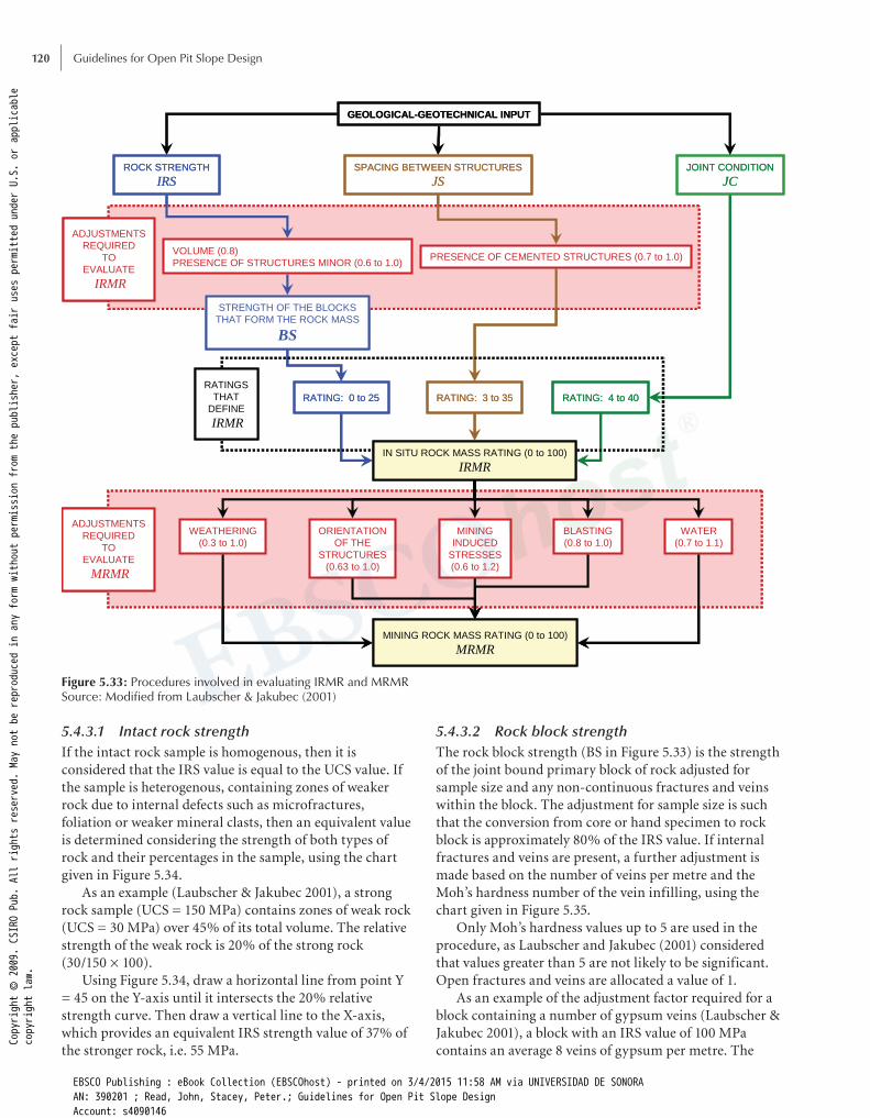
Guidelines for Open Pit Slope Design120
5.4.3.1 Intact rock strengthIf the intact rock sample is homogenous, then it is considered that the IRS value is equal to the UCS value. If the sample is heterogenous, containing zones of weaker rock due to internal defects such as microfractures, foliation or weaker mineral clasts, then an equivalent value is determined considering the strength of both types of rock and their percentages in the sample, using the chart given in Figure 5.34.
As an example (Laubscher & Jakubec 2001), a strong rock sample (UCS = 150 MPa) contains zones of weak rock (UCS = 30 MPa) over 45% of its total volume. The relative strength of the weak rock is 20% of the strong rock (30/150 × 100).
Using Figure 5.34, draw a horizontal line from point Y = 45 on the Y-axis until it intersects the 20% relative strength curve. Then draw a vertical line to the X-axis, which provides an equivalent IRS strength value of 37% of the stronger rock, i.e. 55 MPa.
5.4.3.2 Rock block strengthThe rock block strength (BS in Figure 5.33) is the strength of the joint bound primary block of rock adjusted for sample size and any non-continuous fractures and veins within the block. The adjustment for sample size is such that the conversion from core or hand specimen to rock block is approximately 80% of the IRS value. If internal fractures and veins are present, a further adjustment is made based on the number of veins per metre and the Moh’s hardness number of the vein infilling, using the chart given in Figure 5.35.
Only Moh’s hardness values up to 5 are used in the procedure, as Laubscher and Jakubec (2001) considered that values greater than 5 are not likely to be significant. Open fractures and veins are allocated a value of 1.
As an example of the adjustment factor required for a block containing a number of gypsum veins (Laubscher & Jakubec 2001), a block with an IRS value of 100 MPa contains an average 8 veins of gypsum per metre. The
ROCK STRENGTH
IRSSPACING BETWEEN STRUCTURES
JSJOINT CONDITION
JC
GEOLOGICAL-GEOTECHNICAL INPUT
VOLUME (0.8)
PRESENCE OF STRUCTURES MINOR (0.6 to 1.0)PRESENCE OF CEMENTED STRUCTURES (0.7 to 1.0)
ADJUSTMENTS
REQUIRED
TO
EVALUATE
IRMR
WEATHERING
(0.3 to 1.0)
MINING
INDUCED
STRESSES
(0.6 to 1.2)
RATING: 0 to 25 RATING: 3 to 35 RATING: 4 to 40
STRENGTH OF THE BLOCKS
THAT FORM THE ROCK MASS
BS
IN SITU ROCK MASS RATING (0 to 100)
IRMR
RATINGS
THAT
DEFINE
IRMR
ORIENTATION
OF THE
STRUCTURES
(0.63 to 1.0)
BLASTING
(0.8 to 1.0)
WATER
(0.7 to 1.1)
MINING ROCK MASS RATING (0 to 100)
MRMR
ADJUSTMENTS
REQUIRED
TO
EVALUATE
MRMR
Figure 5.33: Procedures involved in evaluating IRMR and MRMRSource: Modified from Laubscher & Jakubec (2001)
Copyright © 2009. CSI
RO Pub. All rights reserved. May not be reproduced in any form without permission from the publisher, except fair uses permitted under U.S. or applicable
copyright law.
EBSCO Publishing : eBook Collection (EBSCOhost) - printed on 3/4/2015 11:58 AM via UNIVERSIDAD DE SONORAAN: 390201 ; Read, John, Stacey, Peter.; Guidelines for Open Pit Slope DesignAccount: s4090146

Rock Mass Model 121
Jakubec (2001) noted that where there are more than three joints sets, for simplicity they should be reduced to three. If cemented joints form a distinct set and the strength of the cement is less than the strength of the host rock, the rating for open joints is adjusted downwards using the chart given in Figure 5.38.
As an example (Laubscher & Jakubec 2001), if the rating for two open joints at a spacing of 0.5 m was 23, an additional cemented joint with a spacing of 0.85 m would have an adjustment factor of 90%. The final rating would thus be 21, which is equivalent to three open joint sets with an average spacing of 0.65 m.
5.4.3.4 Joint conditionIf the rock mass contains only one set of structures the maximum rating of 40 is adjusted downward in line with relevant factors (see Table 5.27). As an example, if the joints in a single set are curved, stepped and smooth but do not have fillings and the walls are not altered, the adjusted JC rating would be 32 (0.90 × 0.90 × 40). If there
Moh’s hardness of gypsum is 2. The ratio of the vein frequency to fill hardness is thus 4, which provides an adjustment factor on the Y-axis of Figure 5.35 of 0.75. The BS value is thus 60 MPa (0.8 × 0.75 × 100).
Once the BS value has been established, the corresponding rating is applied using the chart in Figure 5.36. For the example given above (BS = 60 MPa), the rating is 18.
5.4.3.3 Joint spacingThe rating for joint spacing (JS) is determined for open joints using the chart given in Figure 5.37. Laubscher and
0 10 20 30 40 50 60 70 80 90 100
Equivalent IRS ( % UCS STRONGER ROCK )
0
10
20
30
40
50
60
70
80
90
100
Wea
ker R
ock
(as
% o
f Tot
al V
olum
e)
0 10 20 30 40 50 60 70 80 90 100
UCSWEAKER ROCK / UCSSTRONGER ROCK (%)
Figure 5.34: Evaluating an equivalent IRS value in the case of heterogenous rock samples of intact rockSource: Laubscher & Jakubec (2001)
0.1 1 10Vein Frequency per metre / Fill Hardness (m-1)
0.60
0.65
0.70
0.75
0.80
0.85
0.90
0.95
1.00
Ad
justm
en
t F
acto
r A
BS
200.2 0.4 0.6 0.8 2 4 6 8 40
Figure 5.35: Adjustment factor for RBS as a function of the Moh’s hardness of the fillings and the frequency of the veins within the rock blockSource: Laubscher & Jakubec (2001)
0 20 40 60 80 100 120 140 160
Rock Block Strength, BS (MPa)
0
5
10
15
20
25
Ra
tin
g
Figure 5.36: Rating values for BSSource: Laubscher & Jakubec (2001)
0.1 1Open-Joint Spacing (m)
0
5
10
15
20
25
30
35
Ra
tin
g
Block Volume (m3)
TWO JOIN
T SETS
ONE JOINT S
ET
THREE JOINT S
ETS
0.2 0.3 0.4 0.5 0.6 0.8 2 3 4 5
0.001 0.008 0.03 0.13 0.34 1 8 27 64 125
Figure 5.37: Rating for open joint spacingSource: Laubscher & Jakubec (2001)
Copyright © 2009. CSI
RO Pub. All rights reserved. May not be reproduced in any form without permission from the publisher, except fair uses permitted under U.S. or applicable
copyright law.
EBSCO Publishing : eBook Collection (EBSCOhost) - printed on 3/4/2015 11:58 AM via UNIVERSIDAD DE SONORAAN: 390201 ; Read, John, Stacey, Peter.; Guidelines for Open Pit Slope DesignAccount: s4090146

Guidelines for Open Pit Slope Design122
is more than one joint, the chart given in Figure 5.39 is used to determine an equivalent rating from the joint sets with the highest and lowest ratings.
As an example of determining an equivalent rating from the joint sets with the highest and lowest rating, assume that the best rating for several joint sets is 36 and the worst is 18, and the worst joints comprise 30% of the total number of joints. The relative rating of the worst to best joints is 50% of the best ones (18/36 × 100).
On Figure 5.39, draw a horizontal line from point Y = 30 on the Y-axis until it intersects the 50% lowest/highest relative rating curve. Then draw a vertical line to the X-axis, which provides an equivalent JC rating of 69% of the value for the best joints, i.e. 25.
5.4.3.5 Establishing MRMR from IRMRTo establish MRMR, the IRMR value is adjusted to account for the effects of weathering, joint orientation, mining-induced stresses, blasting and water. Tables outlining the adjustment factors for weathering, joint orientation, blasting and water are presented in Tables 5.28–5.31. Once the adjustment factors have been determined, the MRMR value is calculated as the product of the IRMR value and the adjustment factors.
Adjustment factors for mining-induced stresses are not tabulated by Laubscher and Jakubec. Mining-induced stresses are recognised by Laubscher and Jakubec (2001) as the redistribution of regional or mine-scale stresses as
Cemented-Joints Spacing (m)
0.70
0.75
0.80
0.85
0.90
0.95
1.00
Ad
justm
en
t F
acto
r,
AJS
0.15 3 1 0.9 0.8 0.6 0.44 2 0.7 0.5 0.3 0.2
Cemented-Joint Sets
ONE
TWO
Figure 5.38: Adjustment factor for cemented joints where the strength of the cement is less than the strength of the host rockSource: Modified from Laubscher &Jakubec (2001)
Table 5.27: Joint condition adjustments for a single joint set
Characteristics of the joints
Adjustment
% of 40
A: Roughness at a large scale
Wavy–multidirectional 1.00
Wavy–unidirectional 0.95
Curved 0.90
Straight/slight undulations 0.85
B: Roughness at a small scale (200 × 200 mm)
Rough–stepped/irregular 0.95
Smooth–stepped 0.90
Slickensided–stepped 0.85
Rough–undulating 0.80
Smooth–undulating 0.75
Slickensided–undulating 0.70
Rough–planar 0.65
Smooth–planar 0.60
Slickensided–planar 0.55
C: Alteration of the rock walls
The rock wall is altered and weaker than the filling 0.75
D: Gouge fillings
Gouge thickness < amplitude asperities of the rock wall
0.60
Gouge thickness > amplitude asperities of the rock wall
0.30
E: Cemented structures/filled joints (infill weaker than rock wall)
Hardness of the infill: 5
0.95
4 0.90
3 0.85
2 0.80
1 0.75
Source: Laubscher & Jakubec (2001)
0 10 20 30 40 50 60 70 80 90 100
"Equivalent" JC Rating (as % of highest JC's rating)
0
10
20
30
40
50
60
70
80
90
100
Lo
we
st
JC J
oin
ts (
as %
of
tota
l)
0 10 20 30 40 50 60 70 80 90 100
Lowest JC Rating / Highest JC Rating
Figure 5.39: Estimating an equivalent rating for JC when the rock mass contains more than one joint setSource: Laubscher & Jakubec (2001)
Copyright © 2009. CSI
RO Pub. All rights reserved. May not be reproduced in any form without permission from the publisher, except fair uses permitted under U.S. or applicable
copyright law.
EBSCO Publishing : eBook Collection (EBSCOhost) - printed on 3/4/2015 11:58 AM via UNIVERSIDAD DE SONORAAN: 390201 ; Read, John, Stacey, Peter.; Guidelines for Open Pit Slope DesignAccount: s4090146

Rock Mass Model 123
of cavability, caving fragmentation and the extent of cave and failure zones.
It is important that the underground origins of the MRMR system are recognised and the appropriate judgments and interpretations made when it is applied to open pit mining situations. For example, as for Bieniawski RMR (Table 5.22), when dealing with pit slope design problems adjustments for joint orientation and groundwater should be unnecessary as both should be accounted for in the stability analyses. Similarly, mining-induced stress and their effect around a large open pit will be different from those underground. Adjustments for the effect of weathering and blasting may be, however, highly relevant in the open pit situation. Overall, the objective is for the engineering geologist, rock mechanics engineer and planning engineer to adjust the IRMR situation.
Finally, it is pointed out that the IRMR procedures and MRMR adjustments described above are the most recently publisheded (Laubscher & Jakubec 2001) and reflect changes since the system was first introduced (Laubscher 1977). As with Bieniawski RMR, it is important that the date of publication is stated if an earlier version of the procedure is being used.
5.4.4 Hoek-Brown GSIThe Hoek-Brown Geological Strength Index (GSI) concept was born in 1980 when it was used in the original Bieniawski RMR (Bieniawski 1974a, 1974b) format in support of the newly developed Hoek-Brown rock mass failure criterion (Hoek & Brown 1980b). Since then it has undergone numerous changes, principally between 1992 and 1995, with the name GSI officially emerging in 1995 (Hoek et al. 1995).
a result of the geometry and orientation of an underground excavation. The adjustment factors are judged to range from as low as 0.60 to as high as 1.20, and their evaluation requires considerable experience of underground mining operations. The example given by Laubscher and Jakubec (2001) is for a caving operation where stresses at a large angle to structures will increase the stability of the rock mass and inhibit caving. In this case the allocated adjustment is 1.20. Conversely, stresses at a low angle will result in shear failure and have an adjustment factor of 0.70.
The example of mining-induced stresses emphasises that the MRMR system was primarily developed from the Bieniawski RMR system to cater for diverse mining situations, principally those underground. The fundamental difference noted by Laubscher (1990) was that the in situ rock mass rating (IRMR) needed to be adjusted according to the mining environment so that the final ratings (MRMR) could be used for mine design. Practical design applications of the MRMR system cited by Laubscher and Jakubec (2001) include the stability of open stopes, pillar design, the determination
Table 5.28: Adjustment factors for the effect of weathering
Degree of weathering
Time of exposure
to weathering (years)
0.5 1 2 3 ≥4
No weathered (fresh) 1.00 1.00 1.00 1.00 1.00
Slightly weathered 0.88 0.90 0.92 0.94 0.96
Moderately weathered 0.82 0.84 0.86 0.88 0.90
Highly weathered 0.70 0.72 0.74 0.76 0.78
Completely weathered 0.54 0.56 0.58 0.60 0.62
Residual soil (saprolite) 0.30 0.32 0.34 0.36 0.38
Source: Laubscher & Jakubec (2001)
Table 5.29: Adjustment factors for the effect of joint orientation
No. joints
defining the
block
No. block faces
inclined from
vertical
JC rating
0–15 16–30 31–40
3 3 0.70 0.80 0.95
2 0.80 0.90 0.95
4 4 0.70 0.80 0.90
3 0.75 0.80 0.95
2 0.85 0.90 0.95
5 5 0.70 0.75 0.80
4 0.75 0.80 0.85
3 0.80 0.85 0.90
2 0.85 0.90 0.95
1 0.90 0.95
Source: Laubscher & Jakubec (2001)
Table 5.30: Adjustment factors for the effect of blasting
Blasting technique Adjustment factor, ABLAST
Mechanical excavation/boring 1.00
Smooth-wall blasting 0.97
Good conventional blasting 0.94
Poor blasting 0.80
Source: Laubscher & Jakubec (2001)
Table 5.31: Adjustment factors for the effect of water
Water condition Adjustment factor, AWATER
Moist 0.95–0.90
Water inflows 25–125 L/min, water pressures 1–5 MPa
0.90–0.80
Water inflows >125 L/min, water pressures >5 MPa
0.70–0.80
Source: Laubscher & Jakubec (2001)
Copyright © 2009. CSI
RO Pub. All rights reserved. May not be reproduced in any form without permission from the publisher, except fair uses permitted under U.S. or applicable
copyright law.
EBSCO Publishing : eBook Collection (EBSCOhost) - printed on 3/4/2015 11:58 AM via UNIVERSIDAD DE SONORAAN: 390201 ; Read, John, Stacey, Peter.; Guidelines for Open Pit Slope DesignAccount: s4090146

Guidelines for Open Pit Slope Design124
The modified format proposed in 1992 was represented in 1993 (Hoek et al. 1993) without any changes except that the rock mass characterisation table was extended to include values for Young’s modulus (E) and Poisson’s ratio (n) (Table 5.32).
Although many practitioners were comfortable with a system based more heavily on fundamental geological observations and less on the numbers provided by the RMR system, probably an equal number regretted that the modification had expunged the numerical accounting of RMR from the rock mass classification process. As a result, in 1995 a numerical system, known as the Geological Strength Index (GSI), was reintroduced and Table 5.32 was replaced (see Table 5.33). The tables are similar except for the addition of GSI to Table 5.33.
The 1992 change (Hoek et al. 1992) is seminal, as it saw the use of RMR discontinued and the rock mass characterised in terms of:
■ the block shapes and the degree of interlock; ■ the surface condition of the intersecting defects.
The principal reason for moving from RMR to the new classification system was that it was judged to be a more adequate vehicle for relating the Hoek-Brown failure criterion to geological observations in the field (Hoek et al. 2002). It was also claimed to overcome an effective double-counting of the uniaxial compressive strength of the intact pieces of rock, which was included in both the RMR classification process and the Hoek-Brown strength computations.
Table 5.32: Hoek-Brown rock mass classification system, 1993
Source: Hoek et al. (1992)Copyright © 2009. CSI
RO Pub. All rights reserved. May not be reproduced in any form without permission from the publisher, except fair uses permitted under U.S. or applicable
copyright law.
EBSCO Publishing : eBook Collection (EBSCOhost) - printed on 3/4/2015 11:58 AM via UNIVERSIDAD DE SONORAAN: 390201 ; Read, John, Stacey, Peter.; Guidelines for Open Pit Slope DesignAccount: s4090146

Rock Mass Model 125
Furthermore, the correlation was developed from 111 tunnelling projects of which half (62) were from Scandinavia and a quarter (28) were from South Africa (Bieniawski 1979), so it is unlikely that it is unique for all geological environments and rock types.
The GSI cut-off value of 25 came about following the realisations that Bieniawski’s RMR was difficult to apply to very poor quality rock masses and that the relationship between RMR and the Hoek-Brown strength criterion m and s parameters (section 5.5.2) was no longer linear when the RMR values were less than 25 (Hoek et al. 1995). The name ‘geological strength index’ was used to stress the importance of fundamental geological observations about the blockiness of the rock mass and
All the GSI values in Table 5.33 greater than 25 are exactly the same as those of the Bieniawski RMR
1976
system. They can be determined visually from surface outcrops, using the chart, or numerically from drill core, using Bieniawski RMR
1976. If Bieniawski RMR
1979 is used,
the GSI value is RMR1979
- 5 (Table 5.32). If neither RMR nor GSI can be directly calculated, a suggested alternative is the empirical relationship between the Barton tunnelling index, Q (Barton et al. 1974), and Bieniawski’s RMR
1976 (Bieniawski 1979):
9 44ln QBieniawski RMR1976= + (eqn 5.53)
This relationship must be used cautiously. The Q-index is used in tunnel design, not open pit mining.
Table 5.33: Hoek-Brown rock mass classification system, 1995
Source: Hoek et al. (1995)
Copyright © 2009. CSI
RO Pub. All rights reserved. May not be reproduced in any form without permission from the publisher, except fair uses permitted under U.S. or applicable
copyright law.
EBSCO Publishing : eBook Collection (EBSCOhost) - printed on 3/4/2015 11:58 AM via UNIVERSIDAD DE SONORAAN: 390201 ; Read, John, Stacey, Peter.; Guidelines for Open Pit Slope DesignAccount: s4090146

Guidelines for Open Pit Slope Design126
the condition of the joint surfaces to the classification system.
Subsequent publications (Hoek & Brown 1997; Marinos & Hoek 2000) saw Table 5.33 modified and issued in the form shown in Table 5.34.
The principal changes between Table 5.33 and Table 5.34 are the presentation of only the GSI values across each box in the table and the introduction of the laminated/sheared rock mass structural classification.
Table 5.34 is now the GSI chart most used in practice. It has been extended to accommodate some of the most variable of rock masses and to project information gained from surface outcrops to depth (Hoek et al. 1998; Marinos & Hoek 2001; Marinos et al. 2005; Hoek et al. 2005).
Attempts have also been made to quantify GSI using joint frequency and orientation statistics (Sonmez & Ulusay 1999; Cai et al. 2004). The variety of these approaches emphasise the need to remember the assumptions that underpin the GSI classification system and the Hoek-Brown strength criterion it supports – that the rock mass is an isotropic clump of intact rock pieces separated by closely spaced joints for which there is no preferred failure direction. As noted in Table 5.34, it follows that the GSI system should not be used when a clearly defined, dominant structural system is evident in the rock mass. This is potentially the case for a number of the rock types nominated in some proposed extensions of the system, including bedded or fissile siltstone, mudstone, shale,
Table 5.34: Hoek-Brown rock mass classification system, 2000
INTACT or MASSIVE‘Intact’ rock specimens.Massive in situ rock with few widelyspaced structures.
BLOCKYWell interlocked undisturbed rockmass consisting of cubical blocksformed by three intersecting setsof structures.
VERY BLOCKYInterlocked, partially disturbed rockmass with multi-faceted angularblocks, formed by four or more setsof structures.
BLOCKY/DISTURBED/SEAMYFolded rock mass with angular blocksformed by many intersecting structuralsets. Persistence of bedding planes orschistosity .
LAMINATED / SHEAREDLack of blockiness due to close
shear planes.
DISINTEGRATEDPoorly interlocked, heavily brokenrock mass with mixture of angularand rounded rock pieces.
VERY
GO
OD
Very
rou
gh, f
resh
unw
eath
ered
sur
face
s.
GO
OD
Roug
h, s
light
ly w
eath
ered
, iro
n st
aine
d su
rfac
es.
FAIR
Smoo
th, m
oder
atel
y w
eath
ered
and
alte
red
surf
aces
.
POO
RSl
icke
nsid
ed, h
ighl
y w
eath
ered
sur
face
s w
ith c
ompa
ctco
atin
gs o
r fil
lings
of a
ngul
ar fr
agm
ents
.
VERY
PO
OR
Slic
kens
ided
, hig
hly
wea
ther
ed s
urfa
ces
with
sof
t cl
ayco
atin
gs o
r fil
lings
.
ROCK MASS STRUCTURE
GEOLOGICAL STRENGTH INDEXJOINTED ROCK MASSES
(modified from Marinos & Hoek (2000))
From the lithology, structure and surface conditionof the structures, estimate the average value ofGSI.
DO NOT try to be too precise. Quoting a range33 ≤ GSI ≤ 37 is more realistic than stating that GSI = 35. Note that this table does not apply tostructurally controlled failures. Where weak planarstructural planes are present in an unfavourable orientation with respect to the excavation face,these will dominate the rock mass behavior.
The shear strength of surfaces in rocks that areprone to deterioration, as a result of changes inmoisture content, will be reduce if water is present.When working with rocks in the fair to very poorcategories, a shift to the right may be made forwet conditions. Water pressure is dealt with byeffective stress analysis.
DEC
REA
SIN
G IN
TERL
OC
KIN
G O
F RO
CK
PIEC
ES
DECREASING SURFACE QUALITY
90
80
70
60
50 40
30
20
10
N/A N/A
N/A N/A
75
3555
.
spacing of weak schistosity or
JOIN
T SU
RFA
CE
CO
ND
ITIO
NS
.
DEC
REA
SIN
G IN
TERL
OC
KIN
G O
F RO
CK
PIEC
ES
DECREASING SURFACE QUALITY
90
80
70
60
50 40
30
20
10
N/A N/A
N/A N/A
75
3555
Source: Marinos & Hoek (2000)
Copyright © 2009. CSI
RO Pub. All rights reserved. May not be reproduced in any form without permission from the publisher, except fair uses permitted under U.S. or applicable
copyright law.
EBSCO Publishing : eBook Collection (EBSCOhost) - printed on 3/4/2015 11:58 AM via UNIVERSIDAD DE SONORAAN: 390201 ; Read, John, Stacey, Peter.; Guidelines for Open Pit Slope DesignAccount: s4090146

Rock Mass Model 127
flysch, schist and gneiss. These rock types should only be accommodated if they have been tectonically damaged and their structural preferences lost.
5.5 Rock mass strength5.5.1 IntroductionHistorically, the Mohr-Coulomb measures of friction (Ø) and cohesion (c) have been used to represent the strength of the rock mass. This practice was based on soil mechanics experience and methodology and assumed that the size of the rock particles in high, closely jointed rock masses were equivalent to an isotropic mass of soil particles. This assumption enabled rock slope design practitioners to adopt the Mohr-Coulomb measures of friction (Ø) and cohesion (c) and led to their embedment in the limit equilibrium stability analysis procedures that were introduced in the 1970s and 1980s. Subsequently, the use of Mohr-Coulomb strength parameters carried over into all the continuum and discontinuum numerical modelling tools that are now common in pit slope design.
It quickly became obvious that obtaining good triaxial measures of friction and cohesion for normal rock masses was not easy. The reasons were various, but usually included:
■ the difficulty of performing tests on rock at a scale at the same order of magnitude as the real thing;
■ the difficulty of getting good undisturbed samples from drill holes cored in rock which was already disturbed or damaged in some way;
■ the scarcity of appropriate triaxial testing equipment and experienced operators;
■ cost.
Initially, the preferred means of overcoming these difficulties was to derive empirical values of friction and cohesion from rock mass classification schemes that were calibrated from experience. The classic example of this practice is the calibration of friction and cohesion against RMR by Bieniawski, as shown in Table 5.35 (Bieniawski 1979, 1989).
Subsequently, many strength criteria were developed for rock (Franklin & Dusseault 1989; Sheorey 1997; Zhang 2005), but the best-known in mining engineering are the Laubscher and the Hoek-Brown rock mass strength criteria. A lesser-known but quite widely used system in open pit mines in North and South America is the CNI criterion developed by Call & Nicholas Inc. (Call et al. 2000).
The Laubscher, Hoek-Brown and CNI criteria are outlined below in sections 5.5.2, 5.5.3 and 5.5.4. They are followed by an outline of a method to account for the directional shear strength of a rock mass (section 5.5.5) and a newly developed synthetic rock mass model that
may provide a means of honouring the strength of the rock mass without relying on Mohr-Coulomb, Hoek-Brown or other such constitutive models (section 5.5.6).
5.5.2 Laubscher strength criteriaThere are two Laubscher criteria, the rock mass strength criterion and the design rock mass strength criterion. Both are intended for use in underground mining.
5.5.2.1 Rock mass strength criterionThe rock mass strength (RMS) is derived from the IRS (section 5.4.3.1) and the IRMR (Figure 5.33 and section 5.4.3.5) according to the following procedure (Laubscher & Jakubec 2001).
The strength of the rock mass cannot be higher than the corrected average IRS of that zone. The IRS has been obtained from the testing of small specimens. However, test work on large specimens shows that large specimens have strengths 80% of the small specimen. As the rock mass is a ‘large’ specimen the IRS must be reduced to 80% of its value. Thus the strength of the rock mass would be IRS × 80% if it had no joints. The effect of the joints and their frictional properties is to reduce the strength of the rock mass.
In the IRMR classification ratings, a rating of 20 is given to all specimens with an IRS greater than 185 MPa because at those high values the IRS has little effect on the relative rock mass strength. On this basis the RMS must be calculated in a similar manner, i.e. that above 185 MPa the value of 200 MPa is used regardless of the IRS value.
Given these conditions, the following procedure is adopted to calculate the rock mass strength.
1 The IRS rating (B) is subtracted from the total rating (A) therefore the balance (i.e. RQD, joint spacing and condition) will be a function of the remaining possible rating of 80.
2 The IRS (C) is reduced to 80% of its value.3 RMS = (A - B) × C × 100.
For example, if the total rating was 60 with an IRS of 100 MPa and a rating of 10:
100 100 5060 10RMS MPa MPa# #= - =] g
Table 5.35: RMR calibrated against rock mass quality and strength
RMR rating Description Ø˚
Cohesion
(kPa)
81–100 Very good rock >45 >400
61–80 Good rock 35–45 300–400
41–60 Fair rock 25–35 200–300
40–21 Poor rock 15–25 100–200
<21 Very poor rock <15 <100
Copyright © 2009. CSI
RO Pub. All rights reserved. May not be reproduced in any form without permission from the publisher, except fair uses permitted under U.S. or applicable
copyright law.
EBSCO Publishing : eBook Collection (EBSCOhost) - printed on 3/4/2015 11:58 AM via UNIVERSIDAD DE SONORAAN: 390201 ; Read, John, Stacey, Peter.; Guidelines for Open Pit Slope DesignAccount: s4090146

Guidelines for Open Pit Slope Design128
5.5.2.2 Design rock mass strength criterionThe design rock mass strength (DRMS) is the unconfined rock mass strength in a specific underground mining environment. An underground mining operation exposes the rock surface and the concern is with the stability of the zone that surrounds the opening. The extent of this zone depends on the size of the opening and, except with mass failure, instability propagates from the rock surface. The size of the rock block generally defines the first zone of instability. Adjustments relevant to the specific mining environment are applied to the RMS to give the DRMS. As the DRMS is in MPa it can be related to the mining-induced stresses. Therefore, the adjustments used are those for weathering, joint orientation and blasting (Tables 5.28–5.30).
For example, for an RMS of 50 and weathering = 85%, orientation = 75% and blasting = 90%, then the total adjustments = 57%:
%5750 29DRMS MPa#= =
5.5.3 Hoek-Brown strength criterionThe Hoek-Brown strength criterion was first published in 1980 (Hoek & Brown 1980a, 1980b) in the form:
/m s’ /’ ’c c1 3 3
1 2)s s s s s= + +_ i (eqn 5.54)
where: ’
1s = major principal effective stress at failure
’3
s = minor effective principal stress at failure
sc = uniaxial compressive strength of the intact rock
m = dimensionless material constant for rock s = dimensionless material constant for rock, ranging from 1 for intact rock with tensile strength to 0 for broken rock with zero tensile strength. c is 0 when the effective normal stress is 0.
In 1992 (Hoek et al. 1992) the criterion was modified to eliminate the tensile strength predicted by the original criterion:
/m’ ’c b c
a1 3 3
)s s s s s= + ^ h (eqn 5.55)
where mb and a are constants for the broken rock. It was
assumed that the jointed rock mass was undisturbed and only its inherent properties were considered. Values of m
b
were estimated by substitution of the value for mi into m
b/
mi (Table 2 in Table 5.36). Values of a were estimated
directly from Table 3 within Table 5.36.In 1995 (Hoek et al. 1995) the criterion was modified
again. The generalised Hoek-Brown criterion was retained in the form of equation 5.55 but was replaced by the GSI. The introduction of GSI also saw the concept of ‘disturbed’ and ‘undisturbed’ rock being dropped. Originally, the ‘disturbed’ Hoek-Brown rock mass strength values were derived by reducing the RMR value
by one row in the classification table, a somewhat arbitrary procedure. Instead, it was decided to let the users make their own judgments of how much to reduce the GSI value to account for the strength loss.
The values of mb/m
i, s and a were set as follows:
For GSI > 25 (undisturbed rock masses):
/m m eb i
GSI28
100=
-c m (eqn 5.56)
s eGSI
9100
=-c m (eqn 5.57)
.a 0 5= (eqn 5.58)
For GSI < 25 (undisturbed rock masses):
s 0= (eqn 5.59)
.a GSI0 65200
= - (eqn 5.60)
The third and final modification was made in 2002 (Hoek et al. 2002), when the values of m
b, a and s were
restated:
m m eb i D
GSI28 14
100= -
-c m (eqn 5.61)
a e e21
61 / /GSI 15 20 3= + -- -] g (eqn 5.62)
s e DGSI
9 3100
= -
-c m (eqn 5.63)
The introduction of the parameter D represents a re-evaluation of the ‘undisturbed’ versus ‘disturbed’ question that in the 1995 generalised equation had been left for the user to decide by making appropriate adjustments to the GSI value. It was reintroduced to represent the degree of disturbance to which the rock mass has been subjected by blast damage and stress relaxation, ranging from D = 0 for undisturbed rock to D = 1 for very disturbed rock masses (Table 5.37). The influence of the parameter can be large and its application requires experience and judgment. Hoek et al. (2002) gave an example using s
ci = 50 MPa, m
i = 10 and GSI = 45. For
D = 0 in a tunnel at a depth of 100 m the derived equivalent friction angle is 47° and the cohesion 580 Pa. For D = 1 in a highly disturbed slope 100 m high the equivalent friction angle is reduced to 28° and the cohesion to 350 kPa. Experience-based starting points for judging the extent of the blast-damaged zone resulting from open-pit mine production blasting are given by Hoek & Karzulovic (2000). Ultimately, the value selected for D should be validated through observation and measured performance.
The procedures for calculating the instantaneous effective friction angle and cohesion values for any particular normal stress are essentially the same as for the generalised 1995 criterion, although the process can be simplified by using the freeware RocLab program
Copyright © 2009. CSI
RO Pub. All rights reserved. May not be reproduced in any form without permission from the publisher, except fair uses permitted under U.S. or applicable
copyright law.
EBSCO Publishing : eBook Collection (EBSCOhost) - printed on 3/4/2015 11:58 AM via UNIVERSIDAD DE SONORAAN: 390201 ; Read, John, Stacey, Peter.; Guidelines for Open Pit Slope DesignAccount: s4090146
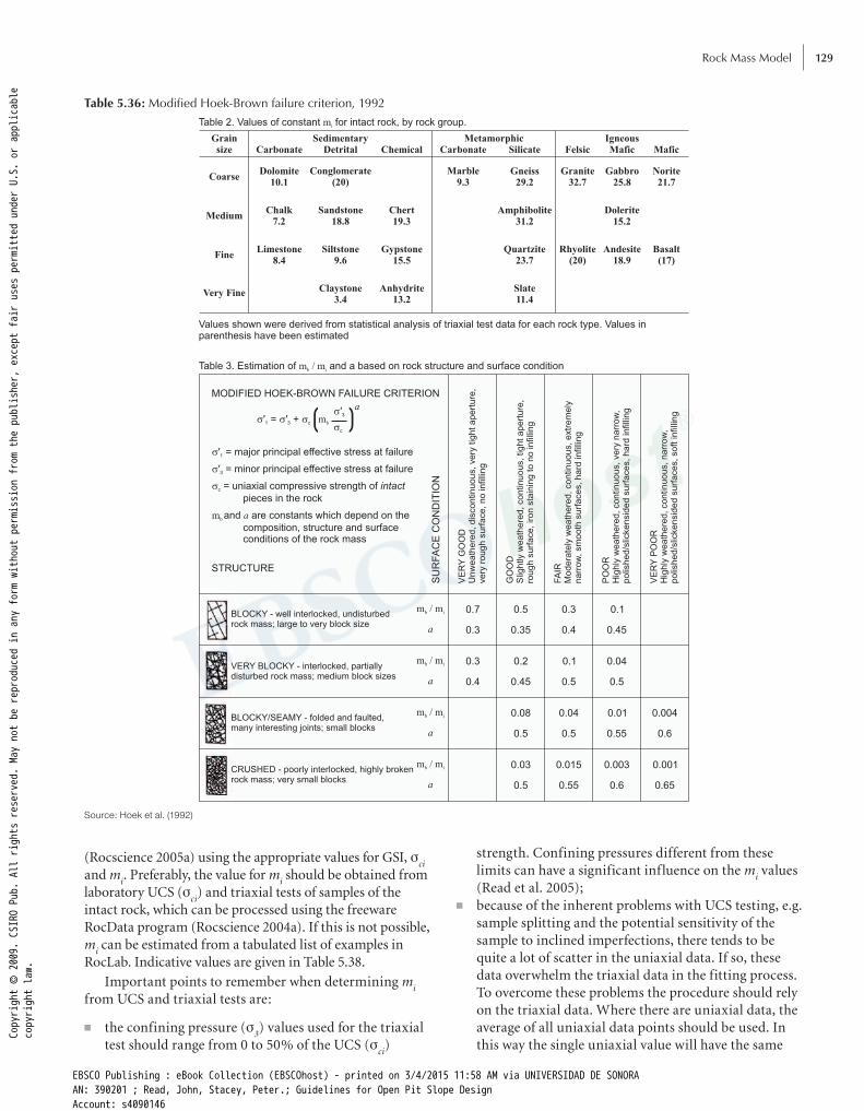
Rock Mass Model 129
(Rocscience 2005a) using the appropriate values for GSI, sci
and mi. Preferably, the value for m
i should be obtained from
laboratory UCS (sci) and triaxial tests of samples of the
intact rock, which can be processed using the freeware RocData program (Rocscience 2004a). If this is not possible, m
i can be estimated from a tabulated list of examples in
RocLab. Indicative values are given in Table 5.38.
Important points to remember when determining mi
from UCS and triaxial tests are:
■ the confining pressure (s3) values used for the triaxial
test should range from 0 to 50% of the UCS (sci)
strength. Confining pressures different from these limits can have a significant influence on the m
i values
(Read et al. 2005); ■ because of the inherent problems with UCS testing, e.g.
sample splitting and the potential sensitivity of the sample to inclined imperfections, there tends to be quite a lot of scatter in the uniaxial data. If so, these data overwhelm the triaxial data in the fitting process. To overcome these problems the procedure should rely on the triaxial data. Where there are uniaxial data, the average of all uniaxial data points should be used. In this way the single uniaxial value will have the same
Table 5.36: Modified Hoek-Brown failure criterion, 1992
Source: Hoek et al. (1992)
Copyright © 2009. CSI
RO Pub. All rights reserved. May not be reproduced in any form without permission from the publisher, except fair uses permitted under U.S. or applicable
copyright law.
EBSCO Publishing : eBook Collection (EBSCOhost) - printed on 3/4/2015 11:58 AM via UNIVERSIDAD DE SONORAAN: 390201 ; Read, John, Stacey, Peter.; Guidelines for Open Pit Slope DesignAccount: s4090146

Guidelines for Open Pit Slope Design130
weight as the triaxial points, which were generally are limited to one value per confining stress (Hoek 2005, editor’s pers comm).
Equations given in Hoek et al. (2002) for determining the Young’s modulus of the rock mass (E
rm) using the GSI
system for values of sci either less than or greater than
100 MPa have been modified by Hoek and Diederichs (2006) into a single equation incorporating both GSI and D:
,/
E MPae
D100 000
11 2
/rm D GSI 1175 25=
+
-+ -
] c ]g mg
(eqn 5.64)
5.5.4 CNI criterionAs an alternative to methods based on RMR assessments, Call & Nicholas Inc. (CNI) developed a criterion that relates the strength of the rock mass directly to the degree of fracturing present in the rock mass through a
Table 5.37: Guidelines for estimating the disturbance factor, D
Source: Hoek et al. (2002)
Copyright © 2009. CSI
RO Pub. All rights reserved. May not be reproduced in any form without permission from the publisher, except fair uses permitted under U.S. or applicable
copyright law.
EBSCO Publishing : eBook Collection (EBSCOhost) - printed on 3/4/2015 11:58 AM via UNIVERSIDAD DE SONORAAN: 390201 ; Read, John, Stacey, Peter.; Guidelines for Open Pit Slope DesignAccount: s4090146

Rock Mass Model 131
Table 5.38: Indicative values for mi for some rocks
Rock
type Class Group
Texture
Coarse(> 2 mm)
Medium
(0.6–2 mm)
Fine
(0.2–0.6 mm)
Very fine
(< 0.2 mm)
SE
DIM
EN
TAR
Y
Clastic Conglomerates® (see Notes)
Sandstones® (15 ± 7)
Siltstones® 7 ± 2
Breccias® (see Notes)
Greywackes® (16 ± 5)
Claystones® 4 ± 2
Shales® (6 ± 2)
Marls® (7 ± 2)
Non-clastic Carbonates Crystalline limestone® (12 ± 3)
Micritic limestone® (9 ± 2)
Sparitic limestone® (10 ± 2)
Dolomites® (9 ± 3)
Evaporites Gypsum® (8 ± 2)
Anhydrite® (12 ± 2)
Organic Chalk® 7 ± 2
ME
TAM
OR
PH
IC
Non-foliated Marble® 9 ± 3
Hornfels® (19 ± 4)
Quartzites® 20 ± 3
Meta-sandstones® (19 ± 3)
Lightly foliated Gneisses® 28 ± 5
Amphibolites® 26 ± 6
Migmatites® (29 ± 3)
Foliated Phyllites® (7 ± 3)
Slates® 7 ± 4
Schists® 12 ± 3
IGN
EO
US
Intrusive Light Granites® 32 ± 3
Diorites® 25 ± 5
Granodiorites® (29 ± 3)
Dark Norites® 20 ± 5
Gabbros® 27 ± 3
Dolerites® (16 ± 5)
Hypabysal Peridotites® (25 ± 5)
Diabases® (15 ± 5)
Porphyries® (20 ± 5)
Volcanics Lavas Rhyolites® (25 ± 5)
Basalts® (25 ± 5)
Obsidians® (19 ± 3)
Dacites® (25 ± 3)
Andesites® 25 ± 5
Pyroclastics Agglomerates® (19 ± 3)
Tuffs® (13 ± 5)
Breccias® (19 ± 5)
Values in brackets are estimates; the others are from triaxial testsSource: Karzulovic (2006)
Copyright © 2009. CSI
RO Pub. All rights reserved. May not be reproduced in any form without permission from the publisher, except fair uses permitted under U.S. or applicable
copyright law.
EBSCO Publishing : eBook Collection (EBSCOhost) - printed on 3/4/2015 11:58 AM via UNIVERSIDAD DE SONORAAN: 390201 ; Read, John, Stacey, Peter.; Guidelines for Open Pit Slope DesignAccount: s4090146

Guidelines for Open Pit Slope Design132
combination of the intact rock strength and the natural fracture strength as a function of RQD (Call et al. 2000).
To determine the modulus of deformation for the rock mass, CNI noted that Bieniawski (1978) proposed the following relationship for the correlation between RQD and the ratio of the rock mass modulus to the intact rock modulus:
/r E Em i
= (eqn 5.65)
where E
m = rock mass deformation modulus
Ei = intact rock deformation modulus
and
r e %RQDa= b] g (eqn 5.66)
for a = 0.225 b = 0.013.
Deere and Miller (1966) demonstrated that the elastic modulus for intact rock can be related to the intact compressive strength, and defined a narrow range of observed ratios between elastic modulus and compressive strength for brittle and soft materials. Consequently, CNI judged it reasonable to expect that a similar relationship could exist between the rock mass modulus and the rock mass strength. Back analysis of slope failures by CNI indicated that the estimation of rock mass strength does follow Bieniawski’s relationship for predicting deformation modulus. However, the strength properties were found to vary according to the square of the modulus ratio, r2. For example, if the square of the modulus ratio r2 is 0.3, the estimated rock mass strength is derived by compositing 30% of the intact rock strength with 70% of the natural fracture strength. The resulting equations for predicting the rock mass friction angle and cohesion are:
For RQD values of >50–60:
C r c r c1m i j
2 2g= + -] g8 B (eqn 5.67)
tan tan tanr r1m i j
1 2 2Q Q Q= + -- ] g8 B (eqn 5.68)
where Ø
m = rock mass friction angle
Cm
= rock mass cohesion c
i = intact rock friction angle
cj = intact rock cohesion
Øj = joint friction angle
cj = joint cohesion
and g = 0.5 to 1.0 g = 0.5, jointed medium to strong rock (>60 MPa) g = 1.0, massive weak to very weak rock (<15 MPa).
For simplicity, the CNI rock mass strength equations were presented for a linear Mohr-Coulomb failure
envelope. However, CNI noted that the rock mass shear strength can be mapped to a power envelope by regression techniques using the calculated percentage of intact rock (r2
* 100) and the power strength envelopes of both the
intact rock and the fracture shear data.The intact compressive strength exerts the primary
control on the constant gamma (g) in equation 5.67. However, the appropriate gamma (g) value is also influenced by the degree of fracturing. In general, the gamma (g) value increases as the intact compressive strength decreases. As the fracture intensity becomes greater, the gamma (g) value lessens.
Applications of equations 5.67 and 5.68 by CNI indicated that for RQD values less than approximately 50, equation 5.68 tended to overpredict the rock mass friction angle. Consequently, the constants alpha (a) and beta (b) in equation 5.66 were revised to provide a better fit to back-calculated rock mass friction angles for lower RQD rock masses. For RQD values of less than 40 and up to 50, these constants are:
■ a = 0.475; ■ b = 0.007.
The two relationships presented for predicting rock mass friction angle do not follow a smooth transition for RQD values between 40 and 60. Modifications to the equations in this RQD range are being investigated by CNI, which hopes to publish results in the future.
Because the relationships presented above for predicting rock mass strength are based on RQD, CNI noted that it is important to recognise that RQD can be an imprecise indicator of the degree of fracturing at RQD values below approximately 20 and above approximately 80. To overcome this deficiency, CNI believe a relationship based on fracture frequency would be preferable. However, existing mine databases typically lack these data or have very limited information. If more extensive databases for fracture frequency become available, CNI considers that these relationships can be readily converted and extended to find wider application in strongly fractured as well as massive rock units (Call et al. 2000).
5.5.5 Directional rock mass strengthThe Hoek-Brown and CNI strength criteria assume that the rock mass comprises an isotropic clump of intact rock pieces separated by closely spaced joints for which there is no preferred failure direction, which is rarely the case. However, using the same concepts of the plane of weakness theory illustrated in Figure 5.40, it is possible to define directional shear strength for the jointed rock mass as follows.
1 Define the basic or isotropic rock mass shear strength by using the generalised Hoek-Brown criterion, and defining equivalent values for the cohesion and friction angle of the rock. This basic strength is the same in all
Copyright © 2009. CSI
RO Pub. All rights reserved. May not be reproduced in any form without permission from the publisher, except fair uses permitted under U.S. or applicable
copyright law.
EBSCO Publishing : eBook Collection (EBSCOhost) - printed on 3/4/2015 11:58 AM via UNIVERSIDAD DE SONORAAN: 390201 ; Read, John, Stacey, Peter.; Guidelines for Open Pit Slope DesignAccount: s4090146

Rock Mass Model 133
directions and in a polar plot defines a circle (Figure 5.41).
2 If there are no discontinuity sets (faults and/or joints) parallel to the slope, then the shear strength of the rock mass can be assumed to be isotropic and corresponds to the basic strength defined in (1).
3 If there are one or more discontinuity sets parallel to the slope, the shear strength of the rock mass cannot be assumed isotropic, because the rock mass is weaker in the direction of these discontinuities. Hence, the rock mass shear strength is much smaller in the direction of these discontinuities and defines a butterfly-shaped curve in a polar plot (Figure 5.41). In the direction normal to the discontinuities the shear strength will be equal to the basic rock mass strength defined in (1), and in the direction parallel to the discontinuities it will be equal to the shear strength of the discontinuities. The shear strength of the discontinuities can be defined according to the following procedure:
→ if the discontinuities are persistent and can be assumed continuous for the slope being studied then the shear strength of the discontinuities can be assessed as described in section 5.3, and values for the cohesion and friction angle of the discontinui-ties can be defined;
→ if the discontinuities are non-persistent and their continuity is interrupted by rock bridges (see Figures 5.42 and 5.43) their shear strength will increase considerably. Unless the effect of rock bridges is accounted for, the shear strength of the discontinuities will be underestimated. Detailed discussions can be found in Jennings (1970, 1972), Einstein et al. (1983) and Wittke (1990). In a rock slope with non-persistent discontinuities a step-path failure surface will occur through a combina-tion of discontinuities and rock bridges (Figure 5.43). An ‘equivalent discontinuity’ can be assigned to this step-path failure (Figure 5.43) and allocated ‘equivalent’ shear strength parameters.
b
S3S3
S1
S1
B
A Slip on
discontinuity
Fracture of rock
Axia
l str
ength
, S 1
0 30 60 90
Angle b
Slip on
discontinuity
b
S3S3
S1
S1
B
A Slip on
discontinuity
Fracture of rock
Axia
l str
ength
, S 1
0 30 60 90
Angle b
Slip on
discontinuity
b
BC
A D
aS3S3
S1
S1
a
b
S1
Four discontinuities at 45o
S1 (kips)120
100
80
60
40
20
0
120
100
80
60
40
20
0
120
100
80
60
40
20
00 15 30 45 60 75 900 15 30 45 60 75 900 15 30 45 60 75 90
Two discontinuities at 60o Three discontinuities at 60o Four discontinuities at 45o
S1 (kips)S1 (kips)
30
20
5
10
30
20
5
10
30
20
5
10
b bb
S3
(kip
s)
S3
(kip
s)
S3
(kip
s)
Four discontinuities at 45o
S1 (kips)120
100
80
60
40
20
0
120
100
80
60
40
20
0
120
100
80
60
40
20
0
120
100
80
60
40
20
0
120
100
80
60
40
20
0
120
100
80
60
40
20
00 15 30 45 60 75 900 15 30 45 60 75 900 15 30 45 60 75 900 15 30 45 60 75 900 15 30 45 60 75 900 15 30 45 60 75 90
Two discontinuities at 60o Three discontinuities at 60o Four discontinuities at 45o
S1 (kips)S1 (kips)
30
20
5
10
30
20
5
10
30
20
5
10
30
20
5
10
30
20
5
10
30
20
5
10
b bb
S3
(kip
s)
S3
(kip
s)
S3
(kip
s)
Figure 5.40: Effect of the pore pressure on (a) one, (b) two and several discontinuities with different orientations on the strength of a rock specimen. (a) Effect of a single discontinuity on the strength of a rock specimen. The plot on the right shows the variation of strength with the orientation of the discontinuity with respect to the direction of loading. (b) Effect of two discontinuities with different inclinations on the strength of a rock specimen. The polar plot on the right shows the variation of strength with the direction of loading with respect to the discontinuities. The perimeter of the blue area defines the directional strength of the rock specimen.Source: Hoek & Brown (1980b)
Copyright © 2009. CSI
RO Pub. All rights reserved. May not be reproduced in any form without permission from the publisher, except fair uses permitted under U.S. or applicable
copyright law.
EBSCO Publishing : eBook Collection (EBSCOhost) - printed on 3/4/2015 11:58 AM via UNIVERSIDAD DE SONORAAN: 390201 ; Read, John, Stacey, Peter.; Guidelines for Open Pit Slope DesignAccount: s4090146
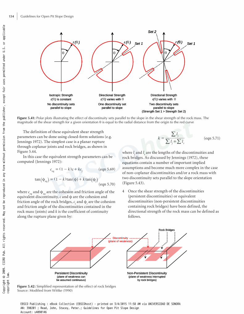
Guidelines for Open Pit Slope Design134
The definition of these equivalent shear strength parameters can be done using closed-form solutions (e.g. Jennings 1972). The simplest case is a planar rupture through coplanar joints and rock bridges, as shown in Figure 5.44.
In this case the equivalent strength parameters can be computed (Jennings 1972):
c k c kc1eq j= - +] g (eqn 5.69)
tan tan tank k1eq j
f f f= - +_ ] ^ _i g h i (eqn 5.70)
where ceq
and feq
are the cohesion and friction angle of the equivalent discontinuity, c and f are the cohesion and friction angle of the rock bridges, c
j and f
j are the cohesion
and friction angle of the discontinuities contained in the rock mass (joints) and k is the coefficient of continuity along the rupture plane given by:
kl l
l
j r
j=
+///
(eqn 5.71)
where lj and l
r are the lengths of the discontinuities and
rock bridges. As discussed by Jennings (1972), these equations contain a number of important implied assumptions and become much more complex in the case of non-coplanar discontinuities and/or a rock mass with two discontinuity sets parallel to the slope orientation (Figure 5.43).
4 Once the shear strength of the discontinuities (persistent discontinuities) or equivalent discontinuities (non-persistent discontinuities containing rock bridges) have been defined, the directional strength of the rock mass can be defined as follows.
Isotropic Strength
r(q) is constant
No discontinuity sets
parallel to slope
q
r (q )
Directional Strength
r(q) varies with qOne discontinuity set
parallel to slope
q
r (q ) Set 1
q
r (q ) Set 1
Set 2
Directional Strength
r(q) varies with
Two discontinuity sets
parallel to slope
(Strength Set 1 > Strength Set 2)
Isotropic Strength
r( ) is constant
No discontinuity sets
parallel to slope
r ( )r ( )
Directional Strength
r( ) varies with
One discontinuity set
parallel to slope
r ( ) Set 1r ( ) Set 1 r (q ) Set 1
Set 2
r (q ) Set 1
Set 2
Directional Strength
r( ) varies with qTwo discontinuity sets
parallel to slope
(Strength Set 1 > Strength Set 2)
Figure 5.41: Polar plots illustrating the effect of discontinuity sets parallel to the slope in the shear strength of the rock mass. The magnitude of the shear strength for a given orientation q is equal to the radial distance from the origin to the red curve
Discontinuity
(plane of weakness)
Rock Bridges
Persistent Discontinuity(plane of weakness can
be assumed continuous)
Non-Persistent Discontinuity(plane of weakness interrupted
by rock bridges)
Discontinuity
(plane of weakness)
Rock Bridges
Persistent Discontinuity(plane of weakness can
be assumed continuous)
Non-Persistent Discontinuity(plane of weakness interrupted
by rock bridges)
Figure 5.42: Simplified representation of the effect of rock bridgesSource: Modified from Wittke (1990)Co
pyright © 2009. CSI
RO Pub. All rights reserved. May not be reproduced in any form without permission from the publisher, except fair uses permitted under U.S. or applicable
copyright law.
EBSCO Publishing : eBook Collection (EBSCOhost) - printed on 3/4/2015 11:58 AM via UNIVERSIDAD DE SONORAAN: 390201 ; Read, John, Stacey, Peter.; Guidelines for Open Pit Slope DesignAccount: s4090146
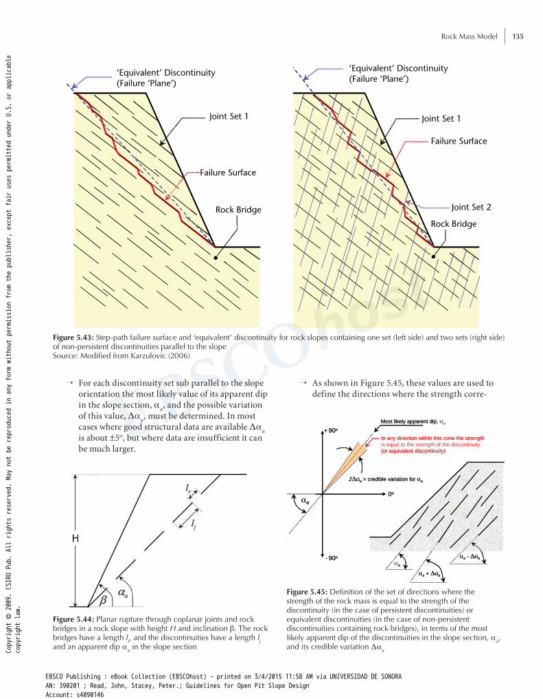
Rock Mass Model 135
→ For each discontinuity set sub parallel to the slope orientation the most likely value of its apparent dip in the slope section, a
a, and the possible variation
of this value, Daa, must be determined. In most
cases where good structural data are available Daa
is about ±5o, but where data are insufficient it can be much larger.
→ As shown in Figure 5.45, these values are used to define the directions where the strength corre-
Rock Bridge
‘Equivalent’ Discontinuity (Failure ‘Plane’)
Joint Set 1
Failure Surface
Joint Set 2
Rock Bridge
‘Equivalent’ Discontinuity (Failure ‘Plane’)
Joint Set 1
Failure Surface
Figure 5.43: Step-path failure surface and ‘equivalent’ discontinuity for rock slopes containing one set (left side) and two sets (right side) of non-persistent discontinuities parallel to the slopeSource: Modified from Karzulovic (2006)
Figure 5.44: Planar rupture through coplanar joints and rock bridges in a rock slope with height H and inclination b. The rock bridges have a length lr, and the discontinuities have a length lj and an apparent dip aa in the slope section
0o
+ 90o
- 90o
Most likely apparent dip, aa
aa
2Daa = credible variation for aa
In any direction within this zone the strength
is equal to the strength of the discontinuity
(or equivalent discontinuity)
aa
aa + Daa
aa - Daa
0o
+ 90o
- 90o
Most likely apparent dip,
aa
2Daa = credible variation for aa
In any direction within this zone the strength
(or equivalent discontinuity)
a
aa + Daa
aa - Daa
Figure 5.45: Definition of the set of directions where the strength of the rock mass is equal to the strength of the discontinuity (in the case of persistent discontinuities) or equivalent discontinuities (in the case of non-persistent discontinuities containing rock bridges), in terms of the most likely apparent dip of the discontinuities in the slope section, aa, and its credible variation DaaCo
pyright © 2009. CSI
RO Pub. All rights reserved. May not be reproduced in any form without permission from the publisher, except fair uses permitted under U.S. or applicable
copyright law.
EBSCO Publishing : eBook Collection (EBSCOhost) - printed on 3/4/2015 11:58 AM via UNIVERSIDAD DE SONORAAN: 390201 ; Read, John, Stacey, Peter.; Guidelines for Open Pit Slope DesignAccount: s4090146
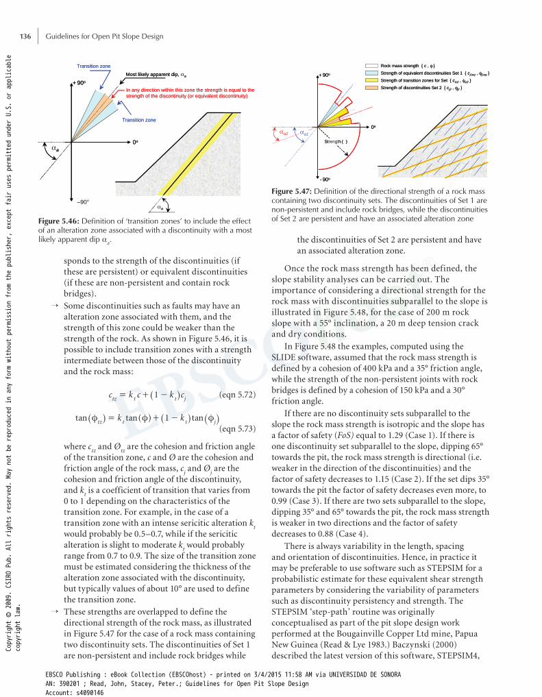
Guidelines for Open Pit Slope Design136
sponds to the strength of the discontinuities (if these are persistent) or equivalent discontinuities (if these are non-persistent and contain rock bridges).
→ Some discontinuities such as faults may have an alteration zone associated with them, and the strength of this zone could be weaker than the strength of the rock. As shown in Figure 5.46, it is possible to include transition zones with a strength intermediate between those of the discontinuity and the rock mass:
c k c k c1tz t t j= + -^ h (eqn 5.72)
tan tan tank k1tz t t j
f f f= + -^ ^ ^ _h h h i (eqn 5.73)
where ctz
and Øtz
are the cohesion and friction angle of the transition zone, c and Ø are the cohesion and friction angle of the rock mass, c
j and Ø
j are the
cohesion and friction angle of the discontinuity, and k
t is a coefficient of transition that varies from
0 to 1 depending on the characteristics of the transition zone. For example, in the case of a transition zone with an intense sericitic alteration k
t
would probably be 0.5–0.7, while if the sericitic alteration is slight to moderate k
t would probably
range from 0.7 to 0.9. The size of the transition zone must be estimated considering the thickness of the alteration zone associated with the discontinuity, but typically values of about 10° are used to define the transition zone.
→ These strengths are overlapped to define the directional strength of the rock mass, as illustrated in Figure 5.47 for the case of a rock mass containing two discontinuity sets. The discontinuities of Set 1 are non-persistent and include rock bridges while
the discontinuities of Set 2 are persistent and have an associated alteration zone.
Once the rock mass strength has been defined, the slope stability analyses can be carried out. The importance of considering a directional strength for the rock mass with discontinuities subparallel to the slope is illustrated in Figure 5.48, for the case of 200 m rock slope with a 55° inclination, a 20 m deep tension crack and dry conditions.
In Figure 5.48 the examples, computed using the SLIDE software, assumed that the rock mass strength is defined by a cohesion of 400 kPa and a 35° friction angle, while the strength of the non-persistent joints with rock bridges is defined by a cohesion of 150 kPa and a 30° friction angle.
If there are no discontinuity sets subparallel to the slope the rock mass strength is isotropic and the slope has a factor of safety (FoS) equal to 1.29 (Case 1). If there is one discontinuity set subparallel to the slope, dipping 65° towards the pit, the rock mass strength is directional (i.e. weaker in the direction of the discontinuities) and the factor of safety decreases to 1.15 (Case 2). If the set dips 35° towards the pit the factor of safety decreases even more, to 0.99 (Case 3). If there are two sets subparallel to the slope, dipping 35° and 65° towards the pit, the rock mass strength is weaker in two directions and the factor of safety decreases to 0.88 (Case 4).
There is always variability in the length, spacing and orientation of discontinuities. Hence, in practice it may be preferable to use software such as STEPSIM for a probabilistic estimate for these equivalent shear strength parameters by considering the variability of parameters such as discontinuity persistency and strength. The STEPSIM ‘step-path’ routine was originally conceptualised as part of the pit slope design work performed at the Bougainville Copper Ltd mine, Papua New Guinea (Read & Lye 1983.) Baczynski (2000) described the latest version of this software, STEPSIM4,
0o
+ 90o
–90°
Most likely apparent dip, aa
aa
In any direction within this zone the strength is equal to the
strength of the discontinuity (or equivalent discontinuity)
aa
Transition zone
Transition zone
0o
+ 90o
Most likely apparent dip, a
a
In any direction within this zone the strength is equal to the
strength of the discontinuity (or equivalent discontinuity)
a
Transition zone
Transition zone
Figure 5.46: Definition of ‘transition zones’ to include the effect of an alteration zone associated with a discontinuity with a most likely apparent dip aa.
0o
+ 90o
- 90o
Rock mass strength { c , f }
Strength of equivalent discontinuities Set 1 { cj1eq , fj1eq }
Strength of transition zones for Set { ctz2 , ftz2 }
Strength of discontinuities Set 2 { cj2 , fj2 }
aa1aa2
Strength ( )
0o
+ 90o
- 90o
Rock mass strength { c , f }
Strength of equivalent discontinuities Set 1 { cj1eq , fj1eq }
Strength of transition zones for Set { ctz2 , ftz2 }
Strength of discontinuities Set 2 { cj2 , fj2 }
aa1aa2
Strength ( )
Figure 5.47: Definition of the directional strength of a rock mass containing two discontinuity sets. The discontinuities of Set 1 are non-persistent and include rock bridges, while the discontinuities of Set 2 are persistent and have an associated alteration zone
Copyright © 2009. CSI
RO Pub. All rights reserved. May not be reproduced in any form without permission from the publisher, except fair uses permitted under U.S. or applicable
copyright law.
EBSCO Publishing : eBook Collection (EBSCOhost) - printed on 3/4/2015 11:58 AM via UNIVERSIDAD DE SONORAAN: 390201 ; Read, John, Stacey, Peter.; Guidelines for Open Pit Slope DesignAccount: s4090146

Rock Mass Model 137
■ Based on the input data for the probability of occur-rence of the Set 1 and Set 2 discontinuities, the program uses a random number-generating technique to check whether one, both or none of the discontinu-ity sets should be simulated in the first cell. If neither of the sets occurs, then rock mass properties are assigned to the first cell.
■ If one or both sets occur, the random number-generat-ing Monte Carlo process is again used to systemati-cally generate the respective discontinuities within the first cell. Based on the input statistical model for discontinuity type for the respective sets, a ‘type’ is assigned to the first structure. A similar process is used to assign orientation (apparent dip), length and shear strength parameters to the first discontinuity and to check whether the discontinuity terminates in rock or is cut-off by another discontinuity. If the first discontinuity is cut-off, then the second discontinuity starts at the end of the first one. If the first discontinu-ity is not cut-off, then an appropriate length rock bridge is simulated at its end. The second discontinu-ity starts at the end of this rock bridge. Depending on their size, such bridges may have either rock or rock mass shear strength assigned by Monte Carlo simula-
which envisages a potential rupture path through a rock slope as a series of adjacent cells (Figure 5.49).
Each cell is statistically associated with one or more of the following failure mechanisms: sliding along adversely oriented discontinuities (Set 1); stepping-up along another steeply dipping discontinuity set (Set 2); or shearing through a rock bridge.
The STEPSIM model assumes that the Set 1 and Set 2 discontinuities occur independently within the rock mass (Baczynski 2000). The computational procedures involve the following basic steps.
■ The user defines the length of the failure path to be evaluated (e.g. 100 m, 250 m, 500 m). For each simu-lated failure path, the structural and strength charac-teristics of each cell are statistically assigned on the basis of the input parameters.
■ A potential failure path starts at the toe of the slope. This position coincides with the first ground condition cell in the simulation process. Cell size should be statistically meaningful and, ideally, should mirror the size of the data windows used for structurally mapping. If this is impossible, an arbitrary cell size may be selected (e.g. 5 × 5 m or 10 × 10 m).
Figure 5.48: Factor of safety of a 200 m rock slope, with an inclination of 55°, for different conditions of rock mass strength
Copyright © 2009. CSI
RO Pub. All rights reserved. May not be reproduced in any form without permission from the publisher, except fair uses permitted under U.S. or applicable
copyright law.
EBSCO Publishing : eBook Collection (EBSCOhost) - printed on 3/4/2015 11:58 AM via UNIVERSIDAD DE SONORAAN: 390201 ; Read, John, Stacey, Peter.; Guidelines for Open Pit Slope DesignAccount: s4090146

Guidelines for Open Pit Slope Design138
tion from the respective input statistical distributions for these parameters. If both Sets 1 and 2 occur in the first cell, the Monte Carlo process is used to decide whether the next discontinuity to be generated should be a Set 1 or a Set 2 member. This process is iterated until the last generated discontinuity or rock bridge terminates at the perimeter or just outside the current cell.
■ The bottom left-hand corner of the second cell starts at the end of the last generated discontinuity or rock bridge. The above simulation process is repeated for the second cell.
■ This process is repeated for successive cells until the target rupture path length has been simulated and the respective shear strength parameters and large-scale roughness characteristics are computed.
■ The process is repeated for a large number of rupture paths (usually 2000–5000) and the ensuing statistical distribution of shear strengths is computed (i.e. a mean and standard deviation for the friction angle and cohesion).
5.5.6 Synthetic rock mass model5.5.6.1 IntroductionAs outlined in section 5.5.1, the Mohr-Coulomb measures of friction (Ø) and cohesion (c) that are used to represent the strength of the rock mass in the limiting equilibrium and continuum and discontinuum numerical modelling slope design tools are derived empirically from various rock mass classification schemes. Although this process is current practice it contains some basic flaws, which can be summarised as follows.
1 Mohr-Coulomb measures friction and cohesion at a point, which we transfer to a three-dimensional body of rock by assuming that the rock mass is isotropic, which is not the case in a jointed rock mass.
2 The empirical friction and cohesion values derived from the most popular classification schemes involve a number of idiosyncrasies and limitations. These include the inbuilt sources of error involved in some parameters used in these schemes (e.g. RQD, section 5.4.2 and GSI, section 5.4.4). As a result there is a high level of uncertainty in the realism of the adopted friction and cohesion values, which we attempt to overcome by calibrating them against existing slope movement data. This severely limits the chances of reliably predicting a future event.
3 We cannot simulate a brittle fracture that can propagate across the joint fabric within the intact pieces of rock (rock bridges) between the structural defects that cut through the rock mass as stress relaxation enables it to dilate and the pieces to separate and move. Instead, the empirical friction and cohesion values are applied as ‘smeared’ or ‘average, non-directional’ parameters across the rock bridges, which are assumed to behave as a continuum.
4 We cannot account for the effect of the degree of disturbance to which the rock mass has been subjected by stress relaxation on the strength of the rock mass (the ‘D’ factor in the Hoek-Brown strength criterion, Table 5.37).
These limitations lead to the recognition of two specific research needs (Read 2007):
■ the need to construct an ‘equivalent material’ that honours the strength of the intact rock and joint fabric within the rock bridges that may occur along a candidate failure surface in a closely jointed rock mass;
■ the need to be able to simulate the brittle fracture that can propagate across the joint fabric within the rock bridges as the rock mass deforms.
These needs and associated questions have formed one of the major research tasks of the Large Open Pit (LOP) Project. A number of approaches and numerical codes with the potential to construct an ‘equivalent material’ and model brittle fracture across the rock bridges were considered. The Itasca PFC code was selected as it uses a micro-mechanics based criterion to model brittle fracture. This offered the potential for stepping away from the Mohr-Coulomb and Hoek-Brown criteria, a feature that was consistent with the research objectives.
5.5.6.2 SRM modelIn PFC the entire model is composed from the start as discrete elements bonded together (the bonded particle method [BPM], Potyondy & Cundall 2004), with the
Figure 5.49: Conceptual STEPSIM4 modelSource: Baczynski (2000)
Copyright © 2009. CSI
RO Pub. All rights reserved. May not be reproduced in any form without permission from the publisher, except fair uses permitted under U.S. or applicable
copyright law.
EBSCO Publishing : eBook Collection (EBSCOhost) - printed on 3/4/2015 11:58 AM via UNIVERSIDAD DE SONORAAN: 390201 ; Read, John, Stacey, Peter.; Guidelines for Open Pit Slope DesignAccount: s4090146

Rock Mass Model 139
inputs (microproperties) restricted to stiffness and strength parameters for the particles and bonds. The initial state of such a bonded assembly of particles is taken as equivalent to an elastic continuum. The fracturing process consists of individual bonds breaking (micro-cracking) and coalescing to form macro-cracks. The PFC assembly is said to exhibit a rich constitutive behavior as an emergent property of the particle assembly without the use of supplied macro-mechanics constitutive models. Extensive tests on simulated laboratory samples have shown that the synthetic PFC material can be calibrated to produce quantitative fits to almost all measured physical parameters, including moduli, strengths and fracture toughness (Potyondy & Cundall 2004).
Development of the BPM method since 2004 in block caving studies by Itasca has shown that the BPM method can represent the strength of the intact rock and joint fabric within the rock bridges with an ‘equivalent material’ or synthetic rock mass (SRM) model (Pierce et al. 2007). In this model the intact rock is represented by an assemblage of bonded particles numerically calibrated using UCS, modulus and/or Poisson’s ratio values to those measured for an intact sample (Figure 5.50). The joints are represented by a smooth joint model that allows associated particles to slide through, rather than over, one another and so represent joints that slide and open in the normal way (Figure 5.51).
Creating and testing the SRM sample illustrated in Figure 5.50 is essentially a three step process: creating the particle assembly that represents the intact rock in PFC3D; generating and importing the discrete fracture network (DFN) that represents the structural pattern of the rock mass into the particle assembly; and testing. Intermediate stages in preparing the sample involve using the DFN to estimate the average size of the rock bridges that will be modelled and calibrating the microproperties of the synthetic material (e.g. particle size distribution and packing, particle and bond stiffness, particle friction coefficients and bond strengths) to the measured properties of the physical material (e.g. Young’s Modulus, UCS). When testing, a minimum of four tests, one tensile,
one UCS and two triaxial tests at differing confining pressures have been found necessary to obtain an estimate of the strength envelope. Changes in the loading direction will also help determine the strength anisotropy of the rock mass. These activities require a working knowledge of one or other of the available DFN modelling packages (e.g. FracMan, JointStats or 3FLO, section 4.4.3), and PFC2D and its 3D equivalent PFC3D (Itasca 2008a, 2008b). To assist users, a Microsoft Excel workbook (the Virtual Lab Assistant or VLA) is available to help with the intact rock calibration process. The workbook can automatically retrieve test results and present them in a separate worksheet, and includes an option to record four predefined videos of each simulation.
From a slope stability point of view the SRM rock bridge is a potential break through. LOP Project research involving the above numerical tensile, UCS and triaxial tests on selected volumes of rock from sponsor mine sites has shown that the SRM does honour the strength of the intact material and the joint fabric within the rock bridges along a candidate failure surface in a closely jointed rock mass, and that it can provide a means of developing a strength envelope that does not rely on either Mohr-Coulomb and/or Hoek-Brown criteria. Similarly, the inverse of providing Hoek-Brown parameters and calibrating the Hoek-Brown strength envelope is possible. Of particular interest is the possibility of adjusting the calibrated Hoek-Brown and/or Mohr-Coulomb strength parameters to specific local conditions, including stress and slope orientation.
So far, the SRM tests have involved eight different rock types and have been performed at laboratory, bench and inter-ramp scales of 5 m, 10 m, 20 m, 40 m and 80 m. Initial outcomes of the research and the perceived benefits of using the SRM model in slope stability analyses are outlined in Chapter 7 (section 7.3.1) and Chapter 10 (section 10.3.3.4). Ongoing research outcomes will be brought into the public domain as they are reported and assessed.
Figure 5.50: SRM model representationSource: Courtesy Itasca Consulting Group, Inc.
Figure 5.51: Smooth joint model representationSource: Courtesy Itasca Consulting Group, Inc.
Copyright © 2009. CSI
RO Pub. All rights reserved. May not be reproduced in any form without permission from the publisher, except fair uses permitted under U.S. or applicable
copyright law.
EBSCO Publishing : eBook Collection (EBSCOhost) - printed on 3/4/2015 11:58 AM via UNIVERSIDAD DE SONORAAN: 390201 ; Read, John, Stacey, Peter.; Guidelines for Open Pit Slope DesignAccount: s4090146

6 HYDROGEOLOGICAL MODELGeoff Beale
6.1 Hydrogeology and slope engineering6.1.1 IntroductionThe presence of groundwater can affect open pit mine excavations in two ways.
1 It can change the effective stress and resulting pore pressures exerted on the rock mass into which the pit slopes have been excavated. Increased pore pressures will reduce the shear strength of the rock mass, increasing the likelihood of slope failures and potentially leading to slope flattening or other remedial measures to compensate for the reduced overall rock mass strength.
2 It can create saturated conditions and lead to standing water within the pit, which may result in:
→ loss of access to all or parts of the working mine area;
→ greater use of explosives, or the use of special explosives and increased explosive failures due to wet blast holes;
→ increased equipment wear and inefficient loading;
→ increased damage to tyres and inefficient hauling;
→ unsafe working conditions.
The main purpose of this chapter is to discuss the first of these aspects – how the presence of groundwater and the resulting pore pressures may affect open pit slope design and performance.
Groundwater usually has a detrimental effect on slope stability. Fluid pressure acting within discontinuities and pore spaces in the rock mass reduces the effective stress, with a consequent reduction in shear strength. This is particularly evident in a weak deformable rock mass, where slope strain softening influenced by fluid pressure can ultimately lead to loss of peak shear strength. In steeper high-strength rock slopes, the potential for sudden
brittle failure under small mining-induced strains is increased when the pore pressure is elevated.
This chapter includes: ■ a discussion of how groundwater relates to pore
pressure, and the relationship to total and effective stress;
■ the main controls on pore pressure and its role in slope engineering;
■ a distinction between general mine dewatering and pit slope depressurisation;
■ a practical explanation of hydrogeology with respect to slope engineering, including the concepts of ground-water flow in fractures (section 6.2);
■ how a conceptual hydrogeological model, which is the fourth and final component of the geotechnical model (Figure 6.1), is developed. Recharge, water table and piezometric surfaces, horizontal and vertical hydraulic gradients, discharge of water to the slope and the resulting pore pressure distribution are addressed in section 6.3;
■ an outline of modelling for numerical hydrogeological models (section 6.4). Section 6.4.2 discusses the normal approach to mine scale numerical hydrogeological modelling. The approach to pit slope scale numerical modelling is outlined in section 6.4.3 and specific numerical modelling procedures for determining the pore pressures in pit slopes are discussed in section 6.4.4;
■ methods that can be used to dissipate pore pressures in the pit slopes (section 6.5).
■ a discussion of topics that need further research (section 6.6).
Definitions of the common terms that apply to groundwater in mine excavations are included in the Glossary.
6.1.2 Porosity and pore pressure6.1.2.1 PorosityWithin most saturated porous formations such as sandstone, siltstone or shale, and within unconsolidated Co
pyright © 2009. CSI
RO Pub. All rights reserved. May not be reproduced in any form without permission from the publisher, except fair uses permitted under U.S. or applicable
copyright law.
EBSCO Publishing : eBook Collection (EBSCOhost) - printed on 3/4/2015 11:58 AM via UNIVERSIDAD DE SONORAAN: 390201 ; Read, John, Stacey, Peter.; Guidelines for Open Pit Slope DesignAccount: s4090146

Guidelines for Open Pit Slope Design142
clastic sediments such as sand, silt and clay, most of the groundwater is contained within the primary interstitial pore spaces of the formation. Hard rock that is weathered or altered may also exhibit interstitial spaces between grains, particularly within zones of clay alteration or weathering. In addition, highly fractured and broken rock may exhibit similar hydrogeological properties to porous strata (commonly referred to as equivalent porous medium). Within porous strata, pore pressure is exerted on the entire rock mass.
The total porosity (n) of the rock mass in these settings is mostly controlled by the interstitial spaces between grains, which typically ranges from 10–30% of the total volume of the formation (n = 0.1 - 0.3) but may be up to 50% (n = 0.5) in poorly consolidated fine-grained materials. A cubic metre of the rock mass may therefore
contain 100–300 L of groundwater. However, particularly for clay materials, the drainable porosity usually represents only a small proportion of the total porosity. Much of the groundwater may be held in place by surface tension and may not freely drain under gravity (Figure 6.2).
Within most saturated competent (hard rock) formations, including igneous, metamorphic, cemented clastic and carbonate settings, virtually all the groundwater is contained within fractures. Because there is no significant primary porosity, the pore pressure is exerted only on the fracture surfaces. However, in addition to the main faults and high-order fracture zones, the rock usually contains abundant low-order small-aperture fracture and joint sets distributed pervasively throughout the rock mass. These micro-fractures also contain groundwater and exhibit pore pressure.
MODELS
DOMAINS
DESIGN
ANALYSES
IMPLEMENTATION
Geology
Equipment
Structure Rock Mass Hydrogeology
GeotechnicalModel
GeotechnicalDomains
StructureStrength
BenchConfigurations
Inter-RampAngles
Overall Slopes
FinalDesigns
Closure
Capabilities
Mine Planning
RiskAssessment
Depressurisation
Monitoring
Regulations
Blasting
Dewatering
Structure
Strength
Groundwater
In-situ Stress
Implementation
Failure Modes
Design Sectors
StabilityAnalysis
Partial Slopes
Overall Slopes
Movement
Design Model
INTE
RA
CTI
VE
PRO
CES
S
Figure 6.1: Slope design process
Copyright © 2009. CSI
RO Pub. All rights reserved. May not be reproduced in any form without permission from the publisher, except fair uses permitted under U.S. or applicable
copyright law.
EBSCO Publishing : eBook Collection (EBSCOhost) - printed on 3/4/2015 11:58 AM via UNIVERSIDAD DE SONORAAN: 390201 ; Read, John, Stacey, Peter.; Guidelines for Open Pit Slope DesignAccount: s4090146