Characterization of community composition and forest structure in a Madagascar lowland rainforest
Eastside Type N Characterization Project Forest Hydrology Study Design
By: Dan Miller and Phil Peterson
December 2009 CMER #08-800

EASTSIDE TYPE N CHARACTERIZATION PROJECT FOREST HYDROLOGY STUDY DESIGN
DECEMBER 2009
PREPARED FOR Scientific Advisory Group Eastside
Cooperative Monitoring Evaluation and Research Committee
by
Dan Miller M2 Environmental Services
Phil Peterson Forest and Channel Metrics

ACKNOWLEDGMENTS
We greatly appreciate the efforts of SAGE in guiding this project, whose members were instrumental in decisions of explanatory variables and identifying available data sets. We also thank Christina Bandaragoda, who provided the SSURGO soils data in a summarized form amenable to GIS analysis for this project. Finally, we are grateful for the always helpful, professional, and thoughtful efforts of Amy Kurtenbach, project manager.

EXECUTIVE SUMMARY
The Forest Hydrology Study is first in a proposed series of studies in the Eastside Type N Characterization Project under the CMER Type N Prescriptions Rule Group. These projects are intended to improve understanding of the geomorphic and ecologic functions filled by Type-N (nonfish-bearing) streams east of the Cascade crest, to identify stream and watershed attributes that control these functions across eastside forested lands addressed by the Forests and Fish Report (FFR), and to characterize human influences on Type-N stream processes and the ecological functions they provide. The Forest Hydrology Study focuses on characterization of base-flow regime; that is, delineation of reaches with perennial and seasonal flow and identification of the physical factors that affect the extent of low-flow surface discharge. Results of the Forest Hydrology Study will guide scoping of future studies in the Eastside Type N Characterization Project.1
The Forest Hydrology Study is divided into design and implementation phases consisting of the following tasks:
Design Phase (presented in this document)
a) Use existing digital data to delineate and characterize Type-N streams and the encompassing Type-N drainage basins to the extent feasible,
b) Use these data to select a representative stratified random sample of Type-N basins for detailed study
Implementation Phase
c) Mapping from digital orthophotos and field surveys for all channels in the selected basins to obtain detailed information not available from existing data, in particular, the presence or absence of surface flow.
d) Identify and quantify relationships between the field-surveyed presence or absence of surface flow with field-measured and air-photo-mapped physical attributes, including measures related to management, and with attributes inferred from analysis of Geographic Information System (GIS) data.
e) Use these data and relationships to develop field-based criteria for delineating seasonal and perennial channels, including estimates of confidence in any such determinations
f) Use these data to develop GIS-based models to estimate the extent of each channel type in all Type-N basins in the study area, including estimates of confidence, and
g) Determine the extent of different base-flow regimes and assess confidence in study results.
This document and accompanying materials 1) describe the conceptual basis for this study design, 2) present a GIS database structure and data for item a above, 3) provide software for obtaining a stratified, equal-probability random sample of Type-N basins for field surveys for 1 The modeling program developed for this study was NOT designed to improve, update, modify, or supplement the current DNR Water Type Layer. This model is only designed to provide a tool to CMER for selecting sites for the Eastside Type N Characterization Project: Forest Hydrology Study’s data collection effort.
East Side Type N Channel Characterization: Forest Hydrology Study Design, December, 2009
item b above, and 4) specifies the measurements and types of analyses required for items c through g above during the study implementation phase.
Eastside FFR lands encompass a vast geographic extent with many Type-N streams. Analyses over this large spatial extent necessitate a Geographic Information System (GIS)-based strategy for the Forest Hydrology Study. GIS topographic analyses are based on existing 10-m digital elevation models (DEMs). Previous studies show that these data are insufficient to resolve site-scale attributes. For example, they cannot resolve all Type-N stream channels. Higher resolution data, such as that obtained from Light Detection and Ranging systems (LiDAR), can potentially resolve site-scale features, but are not available for the entire study area and there are no current plans for widespread State-sponsored collection of such data. The 10-m DEMs resolve larger-scale landscape attributes, many of which impose important controls on stream hydrology and on the processes that transport sediment and organic material from headwater areas to fish-bearing streams. This resolution is sufficient to meet the Forest Hydrology Study objectives. Data analyses during study implementation will establish the confidence with which stream type (seasonal or perennial) can be inferred from available data. Likewise, data collected during study implementation will be available for similar analyses with higher-resolution topographic and other remotely sensed data when these data become available.
GIS data developed during the design phase of this study include a channel network traced from 10-m digital elevation models divided into channel segments (referred to here as reaches) averaging 30-m length. Existing GIS climatic, soils, and geologic data with consistent resolution and completeness over the study area were assembled and used to calculate attributes to quantify characteristics of each reach and of the contributing area to each reach. Channels are grouped by Type-N basins delineated using the watershed to the Type-F-to-N transition point indicated in the water types of the Washington State water-course hydrography (note that the state water type GIS data was updated in May 2009; changes from the previous version are not represented in analyses done for this report).
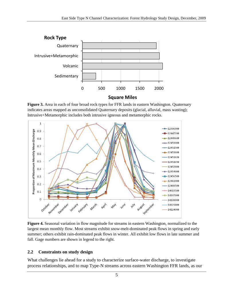
These Type-N basins form the population of sites from which a representative sample of basins for photo mapping and field surveys is selected. Within each sample basin, all Type-N channels will be surveyed (during the implementation phase of the project). Based on previous studies, Type-N basins are stratified over two variables: 1) predominant rock type, divided into four categories with equal numbers of samples in each stratum, and 2) mean annual precipitation, divided into three equal-sized categories with unequal numbers of samples in each stratum. This provides 12 strata. Based on results of Palmquist (2005)2
2 In 2001 CMER initiated the Perennial Initiation Point (PIP) Pilot Study, which was designed to identify where the point of perennial flow began on Type N streams and the size of the basin area associated to the PIP. Although the Forest Hydrology study will collect some information that is similar to what was collected in the 2001 CMER study, this study is NOT related to the PIP Pilot Study nor is it an offshoot of that study. The Forest Hydrology Study is an independent study designed to characterize flow regimes on Type N streams in order to provide the groundwork for future studies needed to validate the Forest Practices Rules implemented on Type N Streams.
, we expect that each strata will require field surveys of about 30 stream channels extending to the channel head or point of upper-most identifiable seasonal flow, for which a total of 100 Type-N basins should be sufficient.
East Side Type N Channel Characterization: Forest Hydrology Study Design, December, 2009
With approval from SAGE and CMER reviewers, it was decided that data collection to characterize temporal patterns (e.g., repeat surveys, gage installation) would be more efficient and likely more successful with data and analysis to characterize spatial controls on base flow. Hence, this study design addresses spatial patterns of base-flow regime. After completion of the study implementation, these data and subsequent analyses will provide a spatial characterization of controls on stream base-flow hydrology, which will inform sample selection for data collection to characterize temporal variability in base flow in subsequent studies.

East Side Type N Channel Characterization: Forest Hydrology Study Design, December, 2009
This page intentionally left blank

TABLE OF CONTENTS
1 INTRODUCTION ............................................................................................................... 11.1 Purpose and Objective of the Eastside Forest Hydrology Study .............................. 21.2 Document Roadmap ..................................................................................................... 2
2 PROJECT DESCRIPTION ............................................................................................... 32.1 Study Area ..................................................................................................................... 32.2 Constraints on study design ......................................................................................... 52.3 A strategy for dealing with these constraints ........................................................... 102.4 Previous Work ............................................................................................................. 152.5 Tasks ............................................................................................................................. 15
3 DESIGN PHASE: GIS TASKS ........................................................................................ 223.1 GIS Data Structure Requirements ............................................................................ 223.2 Data Structure ............................................................................................................. 243.3 Tracing the Channel Network ................................................................................... 253.4 Explanatory Var iables ................................................................................................ 283.5 10-m DEMs versus LiDAR DEMs ............................................................................. 343.6 Stratified Random Sample ......................................................................................... 373.7 Temporal Character istics ........................................................................................... 403.8 GIS Analysis Results ................................................................................................... 403.9 Products to accompany this report ........................................................................... 47
4 REQUIREMENTS FOR PROJECT IMPLEMENTATION ........................................ 484.1 Use of Products from the Forest Hydrology Study .................................................. 484.2 Objectives for data collection ..................................................................................... 514.3 Required Observations ............................................................................................... 524.4 Data Analysis ............................................................................................................... 554.5 Personnel Needs .......................................................................................................... 594.6 Equipment and Software Requirements ................................................................... 614.7 Quality Assurance: ...................................................................................................... 614.8 Timeline: ...................................................................................................................... 614.9 Costs ............................................................................................................................. 61
5 REFERENCES .................................................................................................................. 62
East Side Type N Channel Characterization: Forest Hydrology Study Design, December, 2009
FIGURES AND TABLE
Figure 1. Eastern Washington forested and FFR lands, and locations of unregulated stream gages. .............................................................................................................................4
Figure 2. Cumulative distributions for elevation and mean annual precipitation for eastern Washington FFR lands. ..................................................................................................4
Figure 3. Area in each of four broad rock types for FFR lands in eastern Washington. ..............5
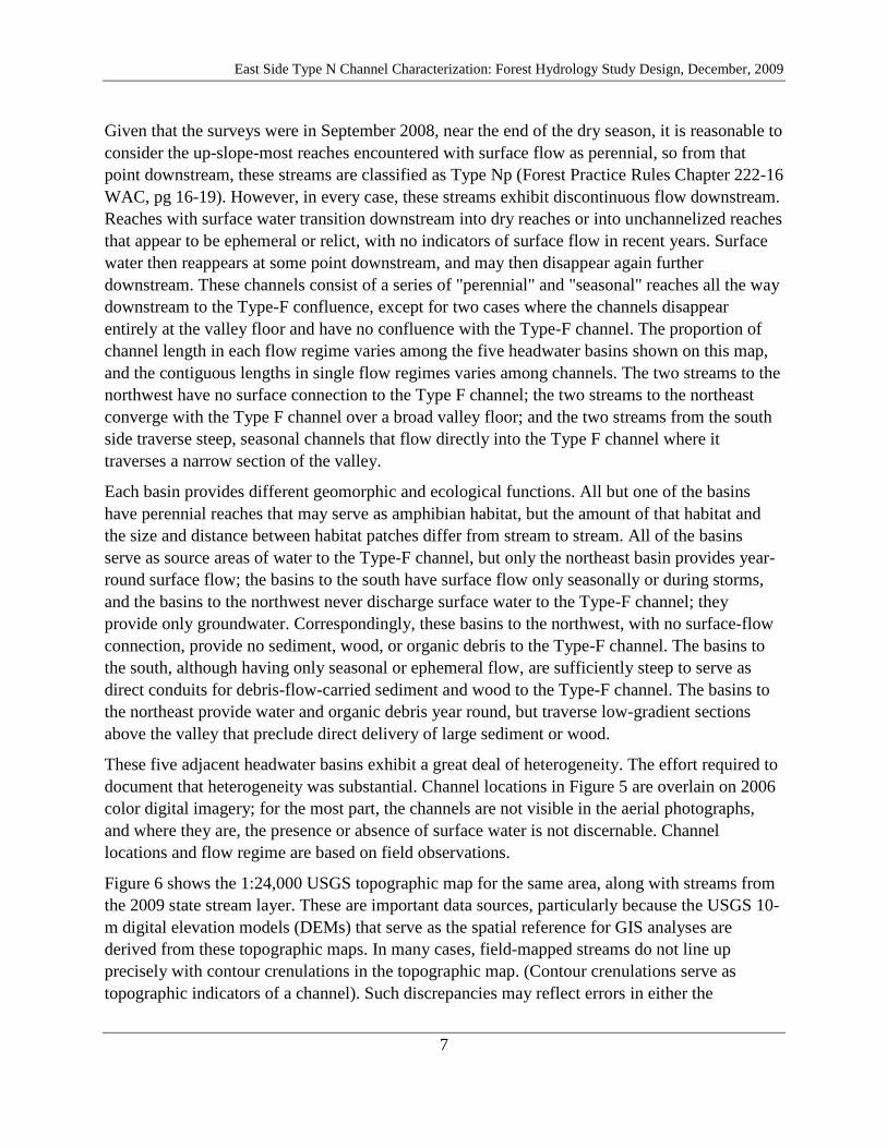
Figure 4. Seasonal variation in flow magnitude for streams in eastern Washington, normalized to the largest mean monthly flow...................................................................................5
Figure 5. Field mapped Type N channels, northeast Washington.................................................6
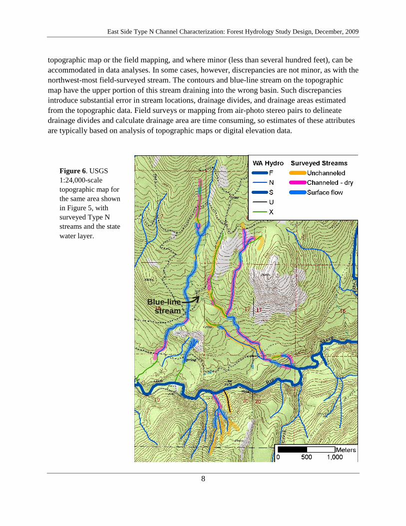
Figure 6. USGS 1:24,000-scale topographic map for the same area shown in Figure 5, with surveyed Type N streams and the state water layer. ......................................................8
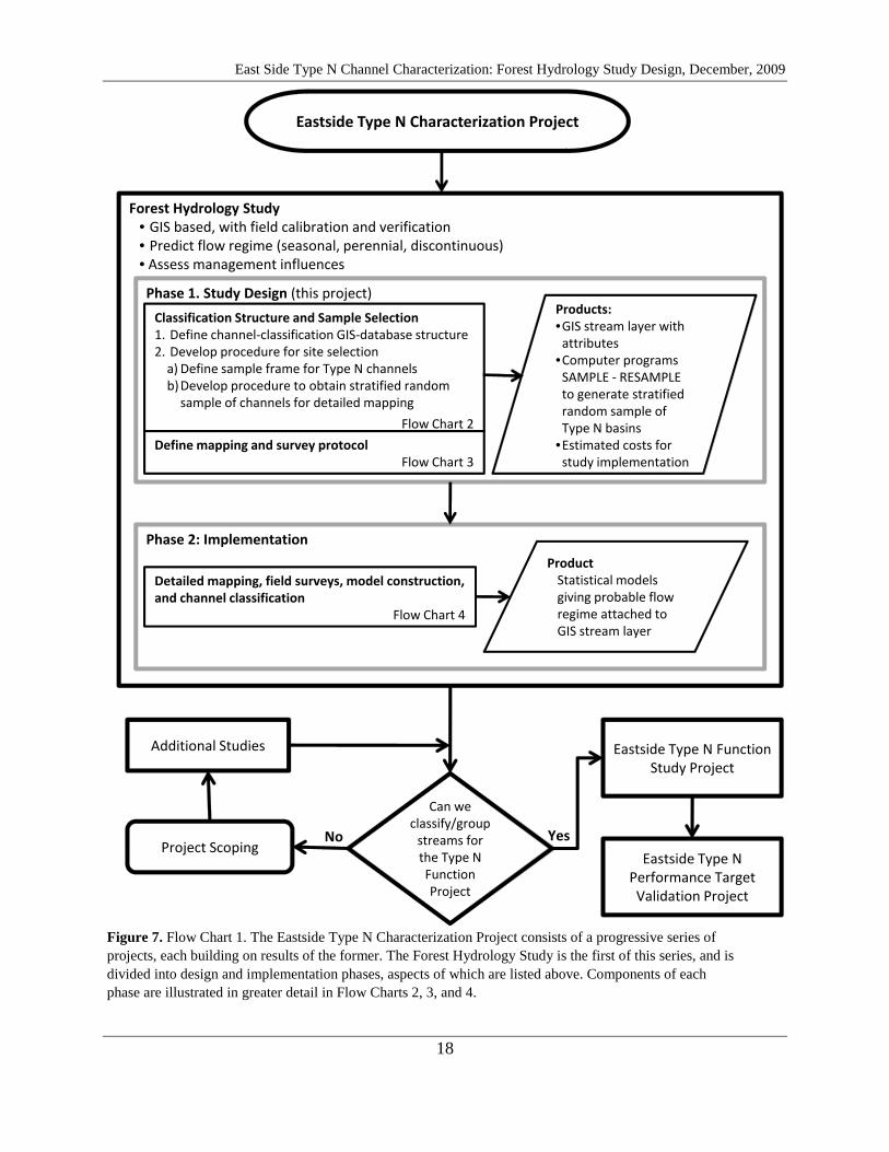
Figure 7. Flow Chart 1. The Eastside Type N Characterization Project consists of a progressive series of projects, each building on results of the former. ...........................................18
Figure 8. Flow Chart 2, Study design, showing the sequence of tasks for designing the GIS channel classification structure. ...................................................................................19
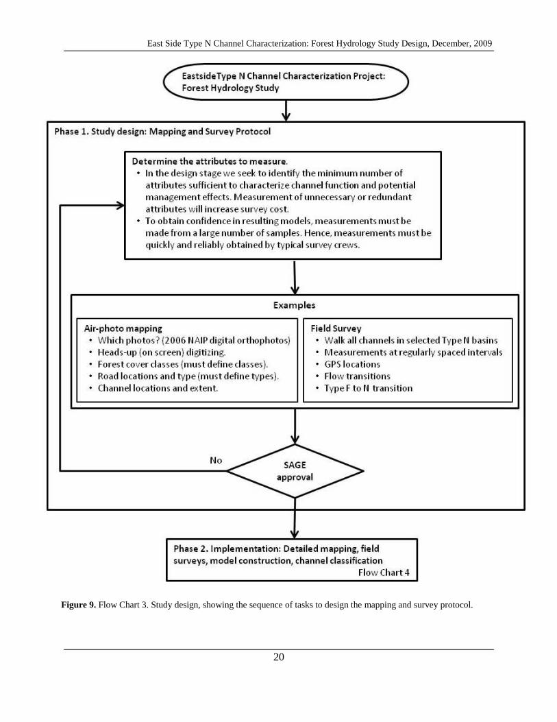
Figure 9. Flow Chart 3. Study design, showing the sequence of tasks to design the mapping and survey protocol.............................................................................................................20
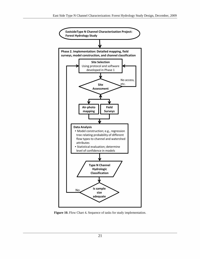
Figure 10. Flow Chart 4. Sequence of tasks for study implementation. .......................................21
Figure 11. Feathering of DEM-traced channels. ...........................................................................28
Figure 12. Type N basins for FFR lands in eastern Washington. .................................................38
Figure 13. Area, channel length, and gradient relationships. ........................................................39
Figure 14. Distribution of rock types and mean-annual precipitation from a stratified probability sample of 100 Type-N basins. ...................................................................40
Figure 15. Climate variables versus mean-annual precipitation for the sample frame of Type N basins............................................................................................................................42
Figure 16. Equal and proportional probability of selecting basins from each stratum. ................43
Figure 17. Distribution of several explanatory variables from the sample frame and for 100 sample basins. .............................................................................................................44
Figure 18. Output from program SAMPLE for estimating study costs and time requirements. ..61
Table 1. Variables linking headwater processes to downstream fish habitat and water quality (SAGE, 2007). ............................................................................................................23
1
1 INTRODUCTION
This report presents a design for the Forest Hydrology Study, the first component of the Eastside Type N3
A detailed discussion of the background and context for this project is contained in RFP08-146 (http://www.dnr.wa.gov/Publications/fp_am_cmer_typen_char_ew_rfp08-146.pdf) and briefly summarized here. Type-N streams compose the majority of stream length (~80%) in a typical Eastern Washington watershed and are recognized as important components of river ecosystems. In particular, perennial (Type Np) streams provide habitat for state-protected amphibians and contribute to downstream water conditions needed to support harvestable levels of salmonids. Hence, Type Np streams receive more extensive riparian protections than those specified for Type Ns streams (WAC 222-30-022(2) at http://www.dnr.wa.gov/Publications/fp_rules_ch222-30wac.pdf). Given the large spatial extent of Type-N streams, determination of the Type Np-to-Ns transition point has significant implications both for timber-harvest planning and for cumulative effects of harvest on watershed condition, leading some stakeholders to request research to examine relationships between current timber-harvest prescriptions specified under the Forest and Fish Report (FFR, available at http://www.dnr.wa.gov/Publications/fp_rules_forestsandfish.pdf) and effects on stream processes that provide ecological functions. SAGE has proposed to undertake this research with a progressive series of projects, starting with the Forest Hydrology Study, which focuses on base-flow hydrology – the factor that delineates Type Np from Type Ns streams.
Characterization Project. These studies are part of a proposed series of research projects under the Cooperative Monitoring Evaluation and Research (CMER) committee’s Type N Riparian Prescriptions Rule Group that are intended to “produce information needed to evaluate the eastern Washington riparian prescriptions to determine if they appropriately protect headwater stream functions” (RFP 08-146 scoping document, pg 3). The Scientific Advisory Group Eastside (SAGE) has defined a strategy for accomplishing this task (see the 2008 CMER workplan at http://www.dnr.wa.gov/Publications/fp_am_cmer_workplan08.pdf), the first aspect of which is characterization of “the physical attributes of eastern Washington streams that are likely to contribute to stream function”: the goal of the Eastside Type N Characterization Project. The Forest Hydrology Study, which seeks to identify base-flow regime (perennial, seasonal, and intermittent) and thereby delineate Type Ns and Type Np streams, is the first component of the Eastside Type N Characterization Project and is addressed by this study design.
3 The Forests and Fish Report (FFR, http://www.dnr.wa.gov/Publications/fp_rules_forestsandfish.pdf) divides Washington streams into three types: shorelines (Type S), fish bearing (Type F), and non-fish bearing (Type N). Type N streams are further divided into those with perennial flow (Type Np) and those with seasonal flow (Type Ns).

East Side Type N Channel Characterization: Forest Hydrology Study Design, December, 2009
2
1.1 Purpose and Objective of the Eastside Forest Hydrology Study
RFP08-146 states:
"The eastern Washington Type N stream research program, including this study, means to improve our knowledge of the character, distribution, and function of these streams in order to help stakeholders agree on appropriate forest practice rules for these stream channels."
Specific to the Forest Hydrology Study:
"The purpose of this study is to contribute to the eastern Washington Type N Characterization, Function, and Effectiveness studies by characterizing hydrologic attributes of eastern Washington lands subject to forest practice rules to determine the extent of various flow regimes and their patterns of occurrence across the landscape.
Study objectives include:
• Determine the spatial and temporal characteristics of surface water discharge in Type N streams across eastern Washington FFR lands.
• Investigate process relationships between stream hydrology, landforms and management activity.
• Develop criteria for characterizing and mapping streams with similar characteristics across the FFR landscape.
Critical Questions
The Eastside Forest Hydrology Study will answer the following questions:
• What are the spatial and temporal characteristics of surface water discharge in Type N streams across eastern Washington FFR lands?
• What landforms, management activities, and/or independent physical characteristics (e.g. geology, climate, etc…) are related to different flow characteristics across eastern Washington FFR lands?
• Is there a set of readily identified external characteristics that can be used to group and/or remotely identify streams that exhibit similar hydrologic characteristics? "
1.2 Document Roadmap
This document defines the tasks and procedures needed to accomplish the objectives and answer the critical questions listed above. Following this introduction, Section 2 provides context for this study, starting with a brief description of the project area and a field example of surveyed

East Side Type N Channel Characterization: Forest Hydrology Study Design, December, 2009
3
Type-N streams in eastern Washington. These examples illustrate the challenges that any effort to characterize flow regime will face, and thereby provide the basis for the research strategy we describe in Section 2.3. This strategy is guided by previous work on similar topics, briefly reviewed in Section 2.4. We close Section 2 with a description of the tasks needed for the Forest Hydrology Study. A large portion of the study design involves use of existing data to characterize eastern Washington Type-N streams and to identify a representative subset of these streams for detailed examination in the implementation phase of the project. These tasks are addressed in Section 3: GIS Tasks for Design Phase, in which we: 1) discuss attributes of an appropriate GIS data structure, 2) describe how available data are used to assemble a set of explanatory variables used to characterize Type-N basins and the channels they contain, 3) describe strategies and methods for identifying a representative sample of these basins, and 4) present results of these analyses. Next, in Section 4: Requirements for Project Implementation, we lay out requirements for the implementation phase of the project, in which we 1) describe the data requirements, 2) list the measurements needed to obtain these data, 3) discuss the analyses that will be required to meet the project objectives, and 4) describe personal and equipment requirements.
Many of the results reported in this document are derived with computer programs written specifically for these tasks. Data outputs are in non-proprietary formats and may be read by any GIS. All programs are written in FORTRAN 95. Source code is available upon request. All maps displayed were made with ArcGIS 9.2.
2 PROJECT DESCRIPTION
2.1 Study Area
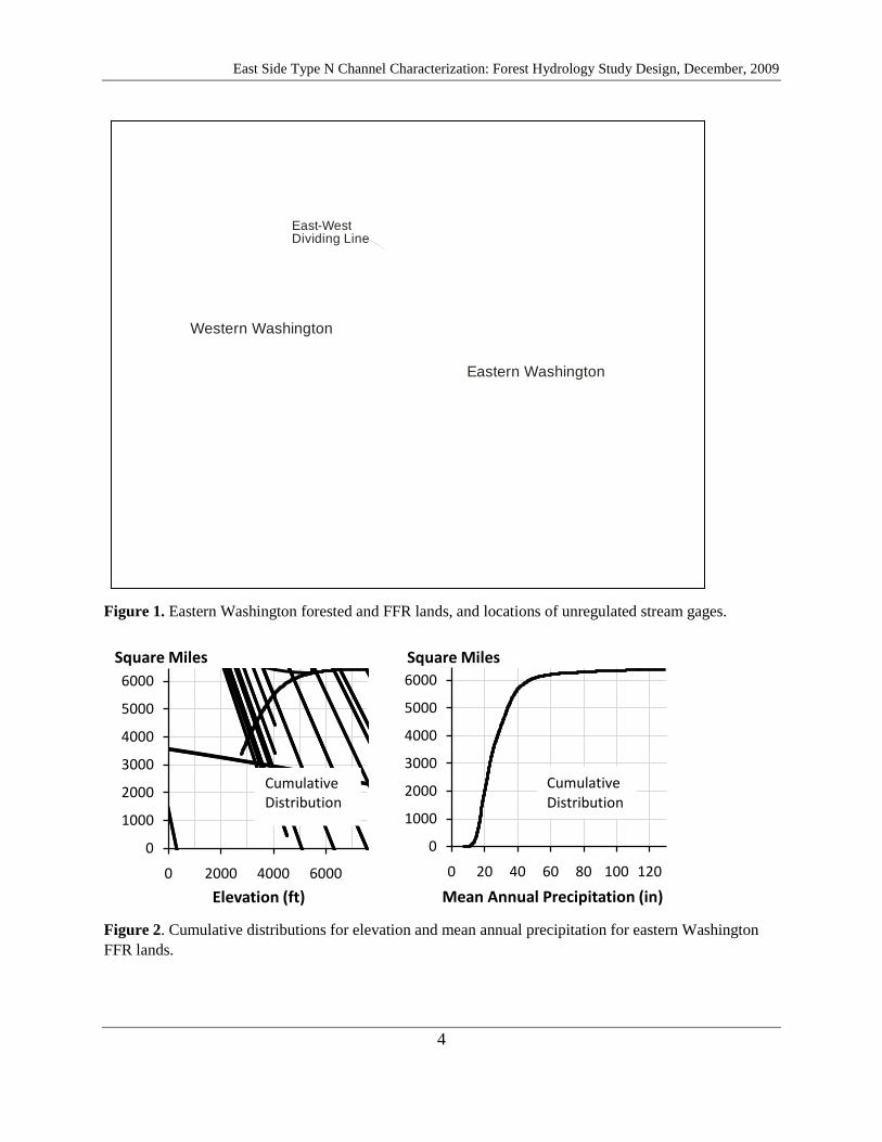
This study addresses eastern Washington forested lands under Forests and Fish Report Rules (FFR), including State-owned lands and areas under Habitat Conservation Plans (HCPs), but excluding tribal lands. Much of eastern Washington is not forested and the majority (~70%) of forested land lies under Federal ownership and is not subject to Forests and Fish Rules (Figure 1). Study objectives specify FFR lands as the focus of this research; hence field surveys will be on Type N basins containing at least some portion of FFR lands and this project will not sample the full range of forest lands across eastern Washington. Even so, as shown in Figures 2 and 3, FFR lands span a large range of elevations, mean annual precipitation depths, and include all major rock types.
Rivers and streams in eastern Washington exhibit seasonal discharge that varies in sync with periods of winter precipitation and spring snow melt, with ground-water supplied base flow typically occurring in late summer and early fall. Some streams experience their lowest discharge during winter when they are frozen. These patterns are illustrated in Figure 4, which shows mean annual monthly discharge for gages in eastern Washington on unregulated rivers and streams (gauge locations are shown in Figure 1).
East Side Type N Channel Characterization: Forest Hydrology Study Design, December, 2009
4
Figure 1. Eastern Washington forested and FFR lands, and locations of unregulated stream gages.
Figure 2. Cumulative distributions for elevation and mean annual precipitation for eastern Washington FFR lands.
East-WestDividing Line
Western Washington
Eastern Washington
0
1000
2000
3000
4000
5000
6000
0 2000 4000 6000
Elevation (ft)
Square Miles
CumulativeDistribution
0
1000
2000
3000
4000
5000
6000
0 20 40 60 80 100 120
Mean Annual Precipitation (in)
Square Miles
CumulativeDistribution
East Side Type N Channel Characterization: Forest Hydrology Study Design, December, 2009
5
Figure 3. Area in each of four broad rock types for FFR lands in eastern Washington. Quaternary indicates areas mapped as unconsolidated Quaternary deposits (glacial, alluvial, mass wasting); Intrusive+Metamorphic includes both intrusive igneous and metamorphic rocks.
Figure 4. Seasonal variation in flow magnitude for streams in eastern Washington, normalized to the largest mean monthly flow. Most streams exhibit snow-melt-dominated peak flows in spring and early summer; others exhibit rain-dominated peak flows in winter. All exhibit low flows in late summer and fall. Gage numbers are shown in legend to the right.
2.2 Constraints on study design
What challenges lie ahead for a study to characterize surface-water discharge, to investigate process relationships, and to map Type-N streams across eastern Washington FFR lands, as our
0 500 1000 1500 2000
Sedimentary
Volcanic
Intrusive+Metamorphic
Quaternary
Square Miles
Rock Type

East Side Type N Channel Characterization: Forest Hydrology Study Design, December, 2009
6
objectives direct us to do? Some clues are provided by a set of Type-N streams in northeast Washington surveyed by Phil Peterson in September 2008. Surveyed streams from five Type-N basins are shown in the map of Figure 5.
Starting from near drainage divides and moving down slope, we find four patterns in the progression from unchanneled hillslopes to channels with flowing surface water:
1) unchanneled swales to dry channels to channels with surface flow,
2) unchanneled swales to channels with surface flow,
3) dry channels to channels with surface flow, and
4) channels starting directly with surface flow.
Figure 5. Field-mapped Type-N channels, northeast Washington.
East Side Type N Channel Characterization: Forest Hydrology Study Design, December, 2009
7
Given that the surveys were in September 2008, near the end of the dry season, it is reasonable to consider the up-slope-most reaches encountered with surface flow as perennial, so from that point downstream, these streams are classified as Type Np (Forest Practice Rules Chapter 222-16 WAC, pg 16-19). However, in every case, these streams exhibit discontinuous flow downstream. Reaches with surface water transition downstream into dry reaches or into unchannelized reaches that appear to be ephemeral or relict, with no indicators of surface flow in recent years. Surface water then reappears at some point downstream, and may then disappear again further downstream. These channels consist of a series of "perennial" and "seasonal" reaches all the way downstream to the Type-F confluence, except for two cases where the channels disappear entirely at the valley floor and have no confluence with the Type-F channel. The proportion of channel length in each flow regime varies among the five headwater basins shown on this map, and the contiguous lengths in single flow regimes varies among channels. The two streams to the northwest have no surface connection to the Type F channel; the two streams to the northeast converge with the Type F channel over a broad valley floor; and the two streams from the south side traverse steep, seasonal channels that flow directly into the Type F channel where it traverses a narrow section of the valley.
Each basin provides different geomorphic and ecological functions. All but one of the basins have perennial reaches that may serve as amphibian habitat, but the amount of that habitat and the size and distance between habitat patches differ from stream to stream. All of the basins serve as source areas of water to the Type-F channel, but only the northeast basin provides year-round surface flow; the basins to the south have surface flow only seasonally or during storms, and the basins to the northwest never discharge surface water to the Type-F channel; they provide only groundwater. Correspondingly, these basins to the northwest, with no surface-flow connection, provide no sediment, wood, or organic debris to the Type-F channel. The basins to the south, although having only seasonal or ephemeral flow, are sufficiently steep to serve as direct conduits for debris-flow-carried sediment and wood to the Type-F channel. The basins to the northeast provide water and organic debris year round, but traverse low-gradient sections above the valley that preclude direct delivery of large sediment or wood.
These five adjacent headwater basins exhibit a great deal of heterogeneity. The effort required to document that heterogeneity was substantial. Channel locations in Figure 5 are overlain on 2006 color digital imagery; for the most part, the channels are not visible in the aerial photographs, and where they are, the presence or absence of surface water is not discernable. Channel locations and flow regime are based on field observations.
Figure 6 shows the 1:24,000 USGS topographic map for the same area, along with streams from the 2009 state stream layer. These are important data sources, particularly because the USGS 10-m digital elevation models (DEMs) that serve as the spatial reference for GIS analyses are derived from these topographic maps. In many cases, field-mapped streams do not line up precisely with contour crenulations in the topographic map. (Contour crenulations serve as topographic indicators of a channel). Such discrepancies may reflect errors in either the
East Side Type N Channel Characterization: Forest Hydrology Study Design, December, 2009
8
topographic map or the field mapping, and where minor (less than several hundred feet), can be accommodated in data analyses. In some cases, however, discrepancies are not minor, as with the northwest-most field-surveyed stream. The contours and blue-line stream on the topographic map have the upper portion of this stream draining into the wrong basin. Such discrepancies introduce substantial error in stream locations, drainage divides, and drainage areas estimated from the topographic data. Field surveys or mapping from air-photo stereo pairs to delineate drainage divides and calculate drainage area are time consuming, so estimates of these attributes are typically based on analysis of topographic maps or digital elevation data.
Blue-linestream
Figure 6. USGS 1:24,000-scale topographic map for the same area shown in Figure 5, with surveyed Type N streams and the state water layer.

East Side Type N Channel Characterization: Forest Hydrology Study Design, December, 2009
9
The state stream layer, in this case, includes the field-mapped stream location. Accuracy of the state stream layer depends on the data source. Where field surveys are available and have been used to update the state data, accuracy can be excellent, as shown in Figure 6. Where stream locations are based on available topographic data, accuracy may not be as good.
These observations show 1) that Type-N streams can exhibit great spatial heterogeneity in flow regime, and 2) that accurate determination of channel locations and presence or absence of surface water requires field surveys. How many channels are there to characterize over eastern Washington FFR lands? Overlaying the state stream layer with the FFR lands indicated in Figure 1 provides a rough estimate: 24,060 miles of Type-N-channel length involving 66,900 separate streams contained within FFR lands. A complete field census is probably beyond the scope of this project.
As seen in Figures 1 through 3, FFR lands are spread discontinuously across a geographic extent that spans a large range in elevation, climate, and geology (and in other factors that affect stream hydrology that we have not included in these figures). We anticipate a corresponding large range in the spatial and temporal characteristics of surface-water discharge in Type-N streams across FFR lands.
An extensive Type-N channel system exhibiting great heterogeneity and located on FFR lands spread discontinuously over all corners of eastern Washington presents formable challenges for the Forest Hydrology Study, whether it is based on field surveys, remotely-sensed data, or GIS analyses. Additionally, for GIS-based analysis, the examples above show that available data contain errors and are of unknown accuracy. These are important considerations in formulating the study design, but there are other, perhaps even more limiting constraints. These involve our ability to detect, even with field surveys, the fundamental controls on Type-N stream hydrology, particularly controls on base-flow regime (perennial, seasonal): the determining factor in delineating Type Np from Type Ns streams.
Base flow derives from groundwater (Winter, 2007). Although overall patterns of groundwater flow reflect regional topography, the local details important to headwater stream hydrology depend on below-ground attributes, things like the depth and stratigraphy of surface deposits and soil, and the orientation, size, and number of bedrock fractures. The transitions in flow regime seen in the streams mapped in Figure 5 may result from meter-scale variations in soil depth, in substrate permeability, and in fracture density and orientation. These factors cannot be mapped from above-ground observations; therefore, these controls on groundwater and stream base flow must be inferred from indicators provided by topography and vegetation. Our ability to resolve relationships between stream-flow characteristics and physical characteristics of the surrounding landscape, even with detailed field-surveys and perfectly accurate GIS data, are thus inherently limited to an extent yet to be determined.
East Side Type N Channel Characterization: Forest Hydrology Study Design, December, 2009
10
2.3 A strategy for dealing with these constraints
To determine characteristics of surface water discharge, to investigate process relationships between stream hydrology, landforms and management activity, and to develop criteria for characterizing and mapping streams with similar characteristics, we must know the location and flow regime for at least some Type-N stream reaches. This requires field mapping. Field mapping is, however, impractical over the entire project domain, so to extend study results across the eastern Washington FFR landscape will also require use of remotely sensed data (e.g., aerial photographs) and GIS analyses. To balance efforts between field surveys, mapping from remotely sensed data, and GIS analyses – or at a more basic level, to decide if these techniques can even provide the information needed to meet the project objectives – we need to know the accuracy and precision of information obtained from each technique. The issues discussed above, however, leave us in a quandary. Even if field mapping were to provide absolute confidence in channel location and flow regime, the confidence with which relationships between hydrology, landforms, and management activity can be resolved is unknown. In addition, the confidence to which channel locations and flow regime can be inferred from remotely sensed and GIS data without field mapping is also unknown. Hence, an important task for this project is to establish boundaries on the levels of confidence attainable with these techniques.
To establish these levels, we define a hierarchical approach for data analysis. Measurements should be made at the finest spatial grain practical. As will be discussed in more detail later, for field mapping this is a 30-m reach and for GIS analysis this is the 10-m horizontal resolution of the USGS DEMs. At this grain, we expect confidence to be low. For example, GIS-based predictions from empirical regression models for the location of a single reach have large uncertainty, as shown by Cupp (2005) in evaluation of the state water-typing model. These fine-grained data can, however, be summed to provide other useful metrics that have a lower level of spatial precision, but a higher level of confidence. For example, we can sum all field-surveyed or GIS-predicted channel lengths to obtain measured or predicted cumulative stream length, which when normalized by drainage area, gives channel density. Channel density is primarily determined by the number and upslope position of channel initiation points (channel heads). Numerous studies have found that channel-head locations, and resulting channel density, vary with climate, geology, topography, and other landscape attributes (e.g., Montgomery and Dietrich, 1989; Palmquist, 2005), so channel density provides a potentially useful variable for discerning variability in the physical controls on surface-water discharge.
Moreover, predictions of cumulative channel length can be made with considerably greater accuracy than predictions of single reach locations. For example, Colson et al. (2006) found that blue-line streams on the USGS topographic maps for headwater stream reaches in North Carolina were within 10-m of field-surveyed locations in only 5 – 17% of the observed cases. Heine et al. (2004), however, found that stream lengths traced from the USGS 10-m DEMs in central Kansas (counting both missed streams and traced streams that didn't actually exist) were 87% accurate. Some reach lengths are under-predicted, others over-predicted. When summed

East Side Type N Channel Characterization: Forest Hydrology Study Design, December, 2009
11
over a large number of reaches, these errors tend to cancel out. Uncertainty in estimates of channel density will, therefore, generally decrease with increasing area (and the corresponding increasing cumulative channel length).
An individual reach defines the fine-grained endpoint for data analysis; channel density of the watershed containing the reach defines the coarse-grained endpoint. We have a range of options in between. Type-N basins, defined as the contributing areas to the Type-N-to-F transition points, provide a logical starting point. Because unconfined water tables reflect smoothed surface topography, each Type-N basin roughly delineates the local groundwater flow system providing base flow to the contained Type-N streams. Comparison of Type-N-basin channel density to measures of basin topography, geology, climate, vegetation cover, and the intensity and type of management activity may thus prove informative and provide sufficient accuracy to give confidence in the results.
Type-N basins come in many sizes, the frequency distribution of which may also be useful information. However, variability in basin size will confound analysis of confidence in data regression and model results because, as stated above, uncertainty in estimates of channel density is inherently a function of basin size. The choice of the Type-N-to-F transition point (which is also uncertain, Cupp, 2005) for defining these basins is, however, an arbitrary decision. We can define headwater basins in any fashion that serves our purpose. Analyses can also be based on basins defined by specified contributing areas. As discussed in greater length in subsequent sections, we use the Type-N-to-F transition points indicated in the state GIS hydrography data to delineate Type-N basins for identifying potential field-survey sites; subsequent analyses can parse these data into smaller sub-basins.
Channel density is a simple starting point for characterizing surface-water discharge. We can use the same strategy of summing reach values to define other metrics that can provide information useful for characterizing stream systems and for identifying the geomorphic and ecologic processes active within these systems. Starting with channel density, we define a series of steps in the hierarchy from coarse- to fine-grained metrics:
• Channel density (channel length per unit area).
• Number of channel heads.
• Proportion of channel length with surface flow.
• Frequency distribution of stream lengths with contiguous flow regime, one for sections with surface flow, one for dry sections.
• Flow regime and contiguous length with that flow type draining to the Type-F channel.
• Location of every 30-m reach
• Flow regime of every 30-m reach

East Side Type N Channel Characterization: Forest Hydrology Study Design, December, 2009
12
Data analyses at each of these levels should include quantitative descriptions of a) variability in observed values, b) scale dependence of that variability (how does the frequency distribution of measured values change with the area over which they are measured), and c) the confidence of predictions at each level. Uncertainty in predicted values will depend both on natural intrinsic variability and on the ability of available data and field observations to resolve the factors that determine reach location and flow regime. Because natural variability is an inherent property of hydrologic systems, predictions need to be phrased in terms of probability. For example, field surveys might include 100 reaches with nearly the same values for all measured physical attributes (drainage area, rock type, forest cover, slope, etc.), yet 80 of these reaches might have surface water and 20 might be dry. The reasons for these differences are not resolved by our observations, so the available data provide only the ability to say that, for other reaches with the same characteristics, we expect an 80% chance that they have surface water and a 20% chance that they are dry.
This series of metrics allows analysis over multiple scales. We can seek regional trends across eastern Washington, we can seek differences among Type-N basins within a region, and we can seek differences among reaches within a Type-N basin. We do not know which level of analysis will prove most useful. We expect, in fact, that each level will provide useful information that can be applied for different purposes.
The metrics we propose for characterizing surface water discharge require continuous surveys of all streams contained within a Type-N basin. Many studies of stream systems use measurements obtained from isolated reaches. That approach, however, does not provide total stream length and can preclude detection of longitudinal patterns in stream attributes, both of which are aspects that we seek to characterize.
Data and data analysis for this project must be spatially explicit, and require use of GIS. A GIS will be used to characterize physical attributes, such as drainage area, or the proportion of basin area in a particular rock type or in particular forest types, to compare to the field-measured values for each of the metrics listed above. These GIS-calculated variables will also be used in predictive models. As noted above, accurate determination of channel location and flow regime require field observations, but field census of all Type-N streams across eastern Washington FFR lands is not practical. Therefore, to characterize surface-water discharge and to map streams with similar characteristics across eastern Washington FFR lands will require models to predict each of the above listed metrics for basins where field observations are not available. These models will be GIS based. Other studies have demonstrated on larger (Type-F) streams that valid inferences about channel characteristics can be made using correlations between GIS-derived and field-measured or air-photo-mapped attributes (Beechie et al., 2006; Clarke et al., 2008; Hall et al., 2007). One task for the Forest Hydrology Study is to extend and evaluate this approach for headwater streams.
East Side Type N Channel Characterization: Forest Hydrology Study Design, December, 2009
13
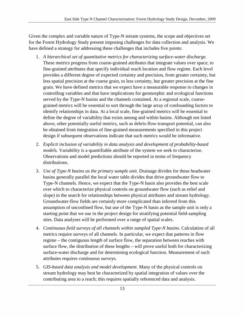
Given the complex and variable nature of Type-N stream systems, the scope and objectives set for the Forest Hydrology Study present imposing challenges for data collection and analysis. We have defined a strategy for addressing these challenges that includes five points:
1. A hierarchical set of quantitative metrics for characterizing surface-water discharge. These metrics progress from coarse-grained attributes that integrate values over space, to fine-grained attributes that specify individual reach location and flow regime. Each level provides a different degree of expected certainty and precision, from greater certainty, but less spatial precision at the coarse grain, to less certainty, but greater precision at the fine grain. We have defined metrics that we expect have a measurable response to changes in controlling variables and that have implications for geomorphic and ecological functions served by the Type-N basins and the channels contained. At a regional scale, coarse-grained metrics will be essential to sort through the large array of confounding factors to identify relationships in data. At a local scale, fine-grained metrics will be essential to define the degree of variability that exists among and within basins. Although not listed above, other potentially useful metrics, such as debris-flow-transport potential, can also be obtained from integration of fine-grained measurements specified in this project design if subsequent observations indicate that such metrics would be informative.
2. Explicit inclusion of variability in data analysis and development of probability-based models. Variability is a quantifiable attribute of the system we seek to characterize. Observations and model predictions should be reported in terms of frequency distributions.
3. Use of Type-N basins as the primary sample unit. Drainage divides for these headwater basins generally parallel the local water table divides that drive groundwater flow to Type-N channels. Hence, we expect that the Type-N basin also provides the best scale over which to characterize physical controls on groundwater flow (such as relief and slope) in the search for relationships between physical attributes and stream hydrology. Groundwater-flow fields are certainly more complicated than inferred from this assumption of unconfined flow, but use of the Type-N basin as the sample unit is only a starting point that we use in the project design for stratifying potential field-sampling sites. Data analyses will be performed over a range of spatial scales.
4. Continuous field surveys of all channels within sampled Type-N basins. Calculation of all metrics require surveys of all channels. In particular, we expect that patterns in flow regime – the contiguous length of surface flow, the separation between reaches with surface flow, the distribution of these lengths – will prove useful both for characterizing surface-water discharge and for determining ecological function. Measurement of such attributes requires continuous surveys.
5. GIS-based data analysis and model development. Many of the physical controls on stream hydrology may best be characterized by spatial integration of values over the contributing area to a reach; this requires spatially referenced data and analysis.

East Side Type N Channel Characterization: Forest Hydrology Study Design, December, 2009
14
Subsequently, extrapolation of empirical results across eastern Washington FFR lands is practicably done only with a GIS-based model.
A large portion of this document focuses on point 5, GIS-based data analysis. In-depth discussion of the other four points awaits data collection during the implementation phase of this project.
In assessing options for study design, it is helpful to remember that the Forest Hydrology Study is observational (not experimental) and inductive (not deductive). We seek spatial trends and empirical relationships between different observed and inferred quantities. Initially, we are neither positing a theory nor posing hypotheses to be tested; we are simply looking to see what is there. Statistical analyses of the data may pose a "null hypothesis"; e.g., there is no relationship between mean annual precipitation and channel density, or there is no relationship between DEM-inferred channel gradient and field-measured channel gradient, but the null hypothesis is simply a framework for identifying relationships in data.
Having said that, we must also admit that we do use a conceptual model of stream hydrology to identify candidate explanatory variables for development of empirical models. This is a necessity of expediency. We seek to distill the innumerable variables that could be defined to those most likely to provide meaningful and significant relationships. We understand that in assuming we know something about the system before we look, we risk biasing study results. However, not doing so would lead to an impractical number of variables to calculate and examine. We feel that previous studies provide sufficient guidance so that the risk of bias is low, but acknowledge that the potential for bias exists and that field personnel and data analysts must be on the lookout for aspects of the system that we have overlooked.
After relationships in data have been inferred statistically, they will then be used to develop empirical models to extrapolate these relationships to basins that do not have channel surveys. Measurements can then be made to compare with these predictions and determine the confidence with which these relationships may be extrapolated. These comparisons provide tests of empirical relationships; not tests of hypotheses deduced from explanations of those relationships. The relationships found in the Forest Hydrology Study may be used, perhaps in future studies, to guide development of possible explanations and to deduce probable cause and effect, at which point we may pose hypotheses, based on those explanations, designed to test and hone our conceptual understanding of the system. Such steps will be essential in efforts to improve knowledge of Type-N systems, but are beyond the scope of the Forest Hydrology Study.
As a final point in discussing strategy, we point out that nowhere in the discussion above do we address temporal variability. Although determination of spatial and temporal characteristics of surface-water discharge is a stated objective for the study, we think that design of a study to determine temporal characteristics should follow results of a study that determines spatial characteristics. We expect that spatially distributed physical attributes, such as rock type, impose important controls on temporal characteristics (Jaeger et al., 2007). That is a hypothesis, and good design of a sampling strategy to test it requires data on the spatial distribution of controlling

East Side Type N Channel Characterization: Forest Hydrology Study Design, December, 2009
15
variables. We will return to this topic, but to avoid confusion, state here that we have not defined measures and metrics to assess temporal variability as part of this project design.
2.4 Previous Work
A substantial body of work precedes and guides this study design (see for example the DNR Type-5 stream literature review at http://www1.dnr.wa.gov/hcp/type5/). Several efforts earlier this decade collected data to characterize the extent of perennial and seasonal flow (Hunter et al., 2005; Jaeger et al., 2007; MacCracken and Boyd, undated report; Pleus and Goodman, 2003; Veldhuisen, 2000, 2004), culminating in the Type N stream demarcation pilot study (Palmquist, 2005). These studies were done to better characterize the extent and controls on Type-N channel base-flow hydrology. They used field surveys to locate the upper-most extent of surface water (the perennial initiation point, or PIP) and evidence of seasonal flow (channel head) during late-summer low-flow periods and used repeat surveys to characterize temporal variability in these points. They then sought to characterize the central tendencies (e.g., mean) and variability of these locations in terms of drainage area, distance to the drainage divide, and distance between the channel head and PIP. Similar studies have been reported in Massachusetts (Bent and Steeves, 2006) and North Carolina (Colson, 2006; North Carolina Division of Water Quality, 2008).
Several researchers have examined the extent of fish use in stream networks using the same or similar data types as used here and their experiences are also useful for this effort. Conrad et al. (2003) developed a GIS-based model, using regressions of observed locations of fish presence or absence to topographic attributes derived from the US Geological Survey 10-m DEMs. Field evaluations of this model (Cupp, 2005; Terrapin Environmental, 2004) indicate substantial reach-scale uncertainties in model predictions, both for channel extent and for fish use. Similar studies are described by Fransen et al. (2006) and by McCleary and Hassan (2008).
Several manuals describing field assessment techniques have been published. The Environmental Protection Agency has published a manual on field techniques for delineating stream reaches with perennial flow from those with seasonal flow (Fritz et al., 2006), and tested these techniques on streams in forested landscapes across the U.S. (Fritz et al., 2008). The Ohio Environmental Protection Agency has published a manual for habitat assessment in Ohio headwater streams, which includes discussion of techniques for determining flow regime (OHEPA, 2002). An interim manual for assessment of streamflow duration in Oregon has recently been released by the Environmental Protection Agency (Topping et al., 2009).
2.5 Tasks
Tasks required for the Forest Hydrology Study may be divided between those addressed by the study design (this document) and those addressed by study implementation, as described below and illustrated in the flow charts of Figures 7 through 10, which illustrate each of the project components and the associated tasks. Flow Chart 1 shows the sequence of steps anticipated for
East Side Type N Channel Characterization: Forest Hydrology Study Design, December, 2009
16
the Eastside Type N Characterization Project, for which the Forest Hydrology Study serves as the first in a potential series of studies. Flow charts 2 through 4 then provide greater detail on each phase and the associated components of the Forest Hydrology Study.
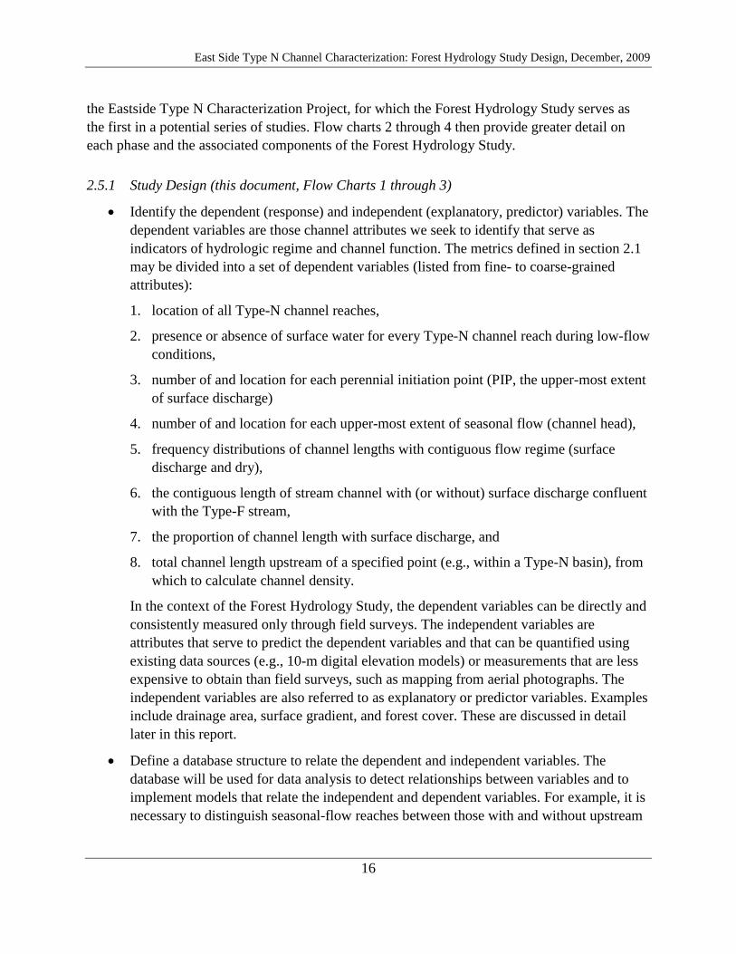
2.5.1 Study Design (this document, Flow Charts 1 through 3)
• Identify the dependent (response) and independent (explanatory, predictor) variables. The dependent variables are those channel attributes we seek to identify that serve as indicators of hydrologic regime and channel function. The metrics defined in section 2.1 may be divided into a set of dependent variables (listed from fine- to coarse-grained attributes):
1. location of all Type-N channel reaches,
2. presence or absence of surface water for every Type-N channel reach during low-flow conditions,
3. number of and location for each perennial initiation point (PIP, the upper-most extent of surface discharge)
4. number of and location for each upper-most extent of seasonal flow (channel head),
5. frequency distributions of channel lengths with contiguous flow regime (surface discharge and dry),
6. the contiguous length of stream channel with (or without) surface discharge confluent with the Type-F stream,
7. the proportion of channel length with surface discharge, and
8. total channel length upstream of a specified point (e.g., within a Type-N basin), from which to calculate channel density.
In the context of the Forest Hydrology Study, the dependent variables can be directly and consistently measured only through field surveys. The independent variables are attributes that serve to predict the dependent variables and that can be quantified using existing data sources (e.g., 10-m digital elevation models) or measurements that are less expensive to obtain than field surveys, such as mapping from aerial photographs. The independent variables are also referred to as explanatory or predictor variables. Examples include drainage area, surface gradient, and forest cover. These are discussed in detail later in this report.
• Define a database structure to relate the dependent and independent variables. The database will be used for data analysis to detect relationships between variables and to implement models that relate the independent and dependent variables. For example, it is necessary to distinguish seasonal-flow reaches between those with and without upstream
East Side Type N Channel Characterization: Forest Hydrology Study Design, December, 2009
17
perennial flow; hence, the database and the statistical models used to predict flow must be structured to predict this relationship.
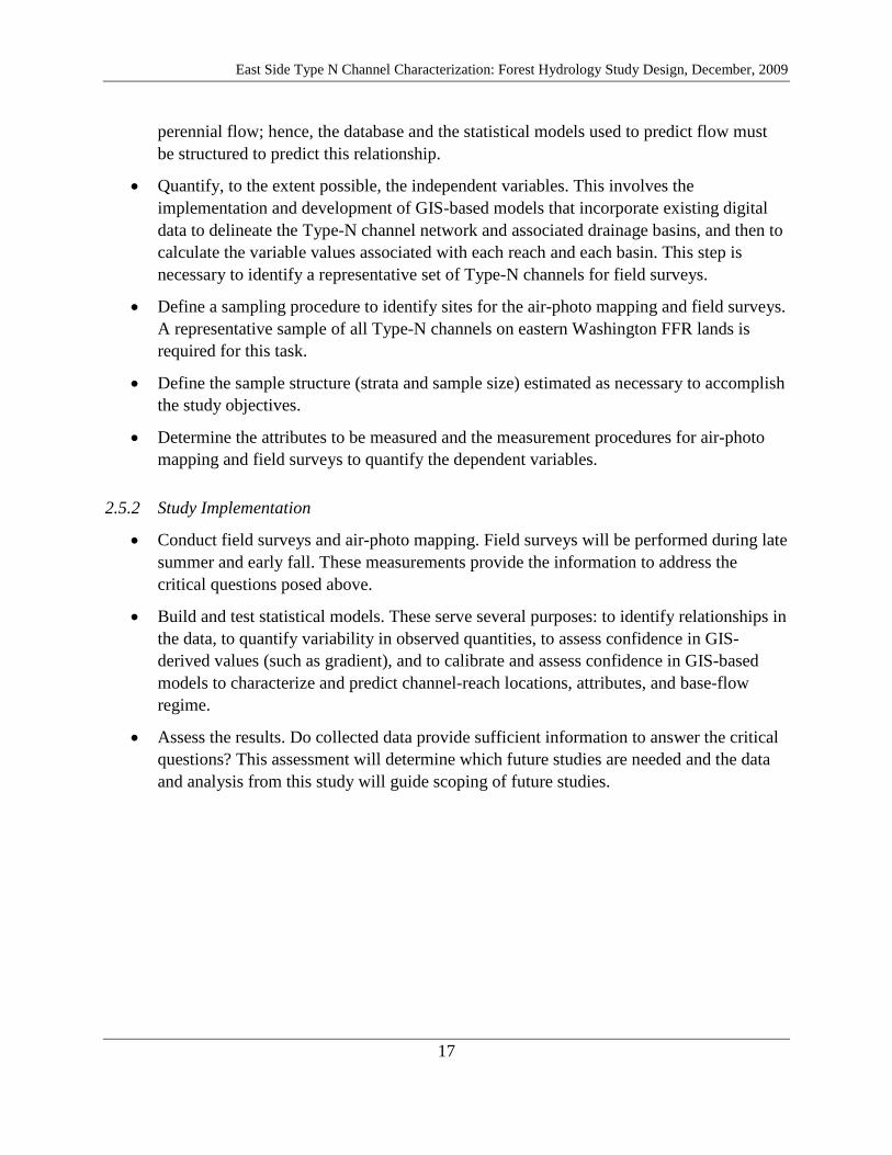
• Quantify, to the extent possible, the independent variables. This involves the implementation and development of GIS-based models that incorporate existing digital data to delineate the Type-N channel network and associated drainage basins, and then to calculate the variable values associated with each reach and each basin. This step is necessary to identify a representative set of Type-N channels for field surveys.
• Define a sampling procedure to identify sites for the air-photo mapping and field surveys. A representative sample of all Type-N channels on eastern Washington FFR lands is required for this task.
• Define the sample structure (strata and sample size) estimated as necessary to accomplish the study objectives.
• Determine the attributes to be measured and the measurement procedures for air-photo mapping and field surveys to quantify the dependent variables.
2.5.2 Study Implementation
• Conduct field surveys and air-photo mapping. Field surveys will be performed during late summer and early fall. These measurements provide the information to address the critical questions posed above.
• Build and test statistical models. These serve several purposes: to identify relationships in the data, to quantify variability in observed quantities, to assess confidence in GIS-derived values (such as gradient), and to calibrate and assess confidence in GIS-based models to characterize and predict channel-reach locations, attributes, and base-flow regime.
• Assess the results. Do collected data provide sufficient information to answer the critical questions? This assessment will determine which future studies are needed and the data and analysis from this study will guide scoping of future studies.
East Side Type N Channel Characterization: Forest Hydrology Study Design, December, 2009
18
Figure 7. Flow Chart 1. The Eastside Type N Characterization Project consists of a progressive series of projects, each building on results of the former. The Forest Hydrology Study is the first of this series, and is divided into design and implementation phases, aspects of which are listed above. Components of each phase are illustrated in greater detail in Flow Charts 2, 3, and 4.
Phase 1. Study Design (this project)
Detailed mapping, field surveys, model construction, and channel classification
Flow Chart 4
Classification Structure and Sample Selection1. Define channel-classification GIS-database structure2. Develop procedure for site selection
a) Define sample frame for Type N channelsb)Develop procedure to obtain stratified random
sample of channels for detailed mapping
Flow Chart 2
Define mapping and survey protocolFlow Chart 3
Products:•GIS stream layer with attributes
•Computer programs SAMPLE - RESAMPLE to generate stratified random sample of Type N basins
•Estimated costs for study implementation
ProductStatistical models giving probable flow regime attached to GIS stream layer
Phase 2: Implementation
Eastside Type N Characterization Project
Forest Hydrology Study• GIS based, with field calibration and verification • Predict flow regime (seasonal, perennial, discontinuous)• Assess management influences
Can we classify/group
streams for the Type N Function Project
Project Scoping
Additional Studies Eastside Type N Function Study Project
Eastside Type N Performance Target Validation Project
No Yes

East Side Type N Channel Characterization: Forest Hydrology Study Design, December, 2009
19
Figure 8. Flow Chart 2, Study design, showing the sequence of tasks for designing the GIS channel classification structure and for obtaining a stratified, random sample of Type-N basins for detailed measurements during the implementation phase.
( Eastside Type N Channel Characterization Project: ') Phase 1. Study design: Mapping
Forest HydroloGY Study and Survey Protocol Flow Chart 3
+ Phase 1. Study design : Classification Structure and Sample Selection
Channel-Classification Structure Identify candidilte variables to use for classifying channels =i"'n
Define GIS-database structure: -Channel reaches " 30m Identi fy and obtain • Explicit redch-to-reach connections available GIS data (a routed netw ork ) "-oDelineation of drainage area to each reach -+ oReach attributes based on: a) loca l Identi fy and develop appropriate GIS models that geomorphology dnd bl conditions within li se available data to ca lculate variable values drainage area to the reach
oTerrestrial sourct' areas linked to Type N linked to Typt' F
1 Each Type N channel i, id entij ied Delineate ~ a,. member of • Type N basin .nd
Type N Yes included variables art' No
the pop ulat ion of Typ e N basins i, potentially sufficient used t o define the sample frame . Basins' as
for channel Cha nnel, .re referen ced t o their watershed to
class ification basins t o include the effect, of Typt'tl / F watershed .ttribute, (ro(k type . transition ~
fore,t (o.er) in the sample frame . point
Site Selection + Define the Silmple Frilme Dbtilin simple rilndom silmple from ItiIch striltum
Identify subset ofTypt' N basins from whidl Set total numbt'r of basins to includt' in samplt'
to obtain a rt'presentativt' sample for Proportion samplt's bt'tween s tr ata
~ dt'tailed mapping. Define thresholds for: • Equal across all strata, or
• Proportion of art'a in FFR land • Proportional to the numbt'r of basins (in the
• Basin Silt' samplt' frdlllt') in each s tr ata
• Total channellt'ngth .-t. .:t SAGE agrt't's that
~ ' geee> "," No sample di stribution No
the sample fr aill e across strata is
is appropriate appropriate
y" Ye>J
Gray -f illed boxe, Site Selection: 'how functions Striltify bilsins by: Gt'ner ate samplt' pro.ided by • Mean annual prt'cipitation SAMPlE,o/tware • Prt'dominant rock typt'
Phase 2.lmplementiltion: Detailed milpping, field surveys, model construction, channel classification
Flow Chart 4
East Side Type N Channel Characterization: Forest Hydrology Study Design, December, 2009
20
Figure 9. Flow Chart 3. Study design, showing the sequence of tasks to design the mapping and survey protocol.
EastsideType N Channel Characterization Project: Forest Hydrolor'{ Study
Philse 1. Study design: Mapping ilnd Survey Protocol
Determine the attributes to measure. . In the design stage we seek to identi fy the minimum number of attributes sufficient to characterize channel function and potential management effects. Measurement of unnecessary or redundant attributes will increase survey cos t. . To obtain confidence in resulting models. measurements must be made from a large number of samples. Hence. measurements must be quickl y and reliably obtained by typka l survey crews.
EMamples
Air-photo mappinli: Field Survey
· Which photos? (2006 fl AIP digital orthophotos) · Walk all channels in selected Type fJ basins
· Heads-up (on screen) digitizing. · Measurements at regularly spaced intervals
· F ores t cover classes (must define classes). · GPS loca tions
· Road loca tions and type (must define types ). · Flow transitions
· Channel loca tions and ex tent. · TypeF to fJ transition
No SAGE approval
Phase 2. Implementation: Detililed mapping, field surveys, model construction, channel classificiltion
Flow Chart 4
East Side Type N Channel Characterization: Forest Hydrology Study Design, December, 2009
21
Figure 10. Flow Chart 4. Sequence of tasks for study implementation.
Phase 2. Implementation: Detailed mapping, field surveys, model construction, and channel classification
Site SelectionUsing protocol and software
developed in Phase 1
Air-photo mapping
Field Surveys
Site Assessment
No access,etc.
Data Analysis• Model construction; e.g., regression tree relating probability of different flow types to channel and watershed attributes
• Statistical evaluation; determine level of confidence in models
Is sample size
adequate
Type N Channel Hydrologic
Classification
No
EastsideType N Channel Characterization Project: Forest Hydrology Study
East Side Type N Channel Characterization: Forest Hydrology Study Design, December, 2009
22
3 DESIGN PHASE: GIS TASKS
3.1 GIS Data Structure Requirements
In designing the Forest Hydrology Study, it is important to consider the larger context for the Eastside Type N Characterization project – characterization of physical attributes that contribute to stream function – because the channel classification and, most importantly, the data structure used to implement and use this classification within a Geographic Information System must serve both to identify hydrologic regime and to characterize stream function. To do so, the key factors that determine Type N stream-channel function must be identified and included in the classification scheme. At this stage in the project, we must rely on existing knowledge and concepts to identify factors that are likely to be important determinants of stream function. The scoping document accompanying RFP 08-146 briefly summarized current understanding of Type N channel processes, which we reiterate here.
Headwater basins compose the majority of the surface area of a watershed. As such, they form the predominant source for surface and ground water, provide habitat for amphibians and invertebrates, and are important sources for sediment, wood, and nutrients to the Type-F channel network. Type-N basin conditions affect water quality; Type-N streams provide unique headwater habitats and form the transport corridors from headwater source areas to Type-F streams. Inputs of water, sediment, nutrients, and wood from Type-N streams influence the hydrology, chemistry, geomorphology, and ecology of Type-F streams. Table 1, from the scoping document in RFP08-146 (reproduced below), lists the factors that control process linkages between Type-N and Type-F stream channels.
From these considerations, we identify three components essential for a stream classification to infer stream function and assess the influence of management actions and forest disturbances on Type-N and downstream Type-F stream channels:
1. The stream classification must characterize the source locations for processes and events that influence the supply of water, sediment, and organic materials to Type-N streams, i.e., each channel reach must have a delineated contributing area. Type-N channels are influenced by the climate, topography, geology, soils, and forest cover of their drainage basins. Existing and obtainable data are insufficient to characterize all pertinent aspects of the source areas to Type N streams, but the classification must be structured to use whatever information about these source areas is available and to incorporate new information that becomes available.
2. The classification must characterize the pathways and transport processes by which water, sediment, and organic materials move to and through Type-N channels. Headwater channels provide the physical link between upslope source areas and fish-bearing streams (Gomi et al., 2002). The processes that move material through these channels (fluvial flow, hyporheic flow, debris flows) and the degree to which materials are stored in headwater valleys

East Side Type N Channel Characterization: Forest Hydrology Study Design, December, 2009
23
determine the rate at which materials originating upslope are carried to fish-bearing channels (Lancaster and Casebeer, 2007; Miller and Burnett, 2008). The classification must include information characterizing flow paths from source locations to fish-bearing streams, including attributes pertinent to sediment transport process (fluvial or mass-wasting) and sediment storage potential (gradient, valley width).
3. The classification must characterize the response of Type-F channels to inputs from Type-N streams. The response of a Type F channel to inputs from Type N channels depend on the type and magnitude of those inputs and on geomorphic attributes of the Type-N and Type-F streams. Factors affecting this response include position in the channel network (e.g., the size of the Type F channel relative to the Type N), the density (number per unit length) of Type N tributary junctions, valley geometry (which determines the space available for storage of sediment in fans, terraces, floodplains and upstream of obstructions such as wood jams), the nature of material provided by Type N streams (e.g., boulders or sand, large wood or no wood), and the timing, magnitude, and frequency of these inputs (Benda et al., 2004a; Benda et al., 2004b). The classification must include attributes pertinent to Type F channel response to inputs from tributary Type N channels.
Such a stream classification system is of greater scope than required for the Forest Hydrology Study: the factors that affect flow regime fall within the domain of components one and two. To assess the consequences of timber harvests, roads, and natural forest disturbances for headwater and downstream fish-bearing channel systems, all three components are needed to link cause and effect. Because the Forest Hydrology Study is the first in a potential series of studies to address these issues, it is worthwhile to recognize and accommodate these requirements now.
Table 1. Variables linking headwater processes to downstream fish habitat and water quality (SAGE, 2007). Key variable
Factors controlling connectivity to F segment
Factors or conditions in N segment that influence significance of key variable on downstream F segment habitat and water quality
Factors or conditions influencing significance of F segment response
Summer water temperature
• flow regime (perennial, intermittent, ephemeral)
• discharge (summer low flow) • shade / wind • depth • groundwater input • hyporheic exchange
• discharge (summer low flow)
Sediment supply
• flow regime • gradient • channel confinement • storage potential
• discharge (peak) • flood potential • basin size • bank erosion potential
• discharge (peak) • gradient • channel confinement • position in stream network
LWD supply • debris flow or fluvial dominated
• channel confinement • storage potential
• discharge (peak) • flood potential • basin size • bank erosion potential
• discharge (peak) • gradient • channel confinement
Food Supply/ Nutrients
• flow regime • discharge (all) • riparian tree composition • geomorphology • LWD supply
• discharge (all) • position in stream network • fish community composition

East Side Type N Channel Characterization: Forest Hydrology Study Design, December, 2009
24
3.2 Data Structure
To link source areas, headwater (Type N), and fish-bearing (Type F) channels, we need to determine the flow paths for water and mass-wasting debris that connect these different areas. Hence, a digital elevation model (DEM), from which flow directions can be inferred, provides the base layer to which all other data types are referenced. Channel locations and contributing areas to channel segments are based on DEM-determined flow paths. DEM-traced channels are stored in a shapefile (ESRI, 1998), a data format that can be read by a GIS. Channels are divided into reaches of approximately 30-m length. This short reach length is used for two reasons: it is possible to aggregate information into longer reaches, if desired, and it allows us to compare the variability resolved from the DEM to that observed on the ground. Attributes for each reach (e.g., drainage area, mean annual precipitation for that drainage area) are stored as tabular data files that can be read by a GIS or other database software (e.g., a spreadsheet such as Microsoft Excel). Included in this list of attributes are the up- and down-stream reach ID numbers, so that connectivity through the channel network can be determined. In GIS terminology, this is a “routed” channel network, from which we can determine such things as which Type F channel reach each Type N reach ultimately drains to, the distance from each Type N reach to the confluence with a Type F reach, and attributes of each intervening Type N reach. Each reach can thereby be classified not only in terms of its local attributes, but also in terms of the attributes of up- and downstream reaches. For example, we can subsequently predict reaches likely to have perennial flow upstream and seasonal flow downstream.
Because all data layers are referenced to the DEM, all non-channel areas can be classified in terms of the channel reach they drain to. This provides an explicit linkage between source areas and channel reaches. Reaches can thereby be classified in terms of attributes of their contributing areas, such as mean annual precipitation or predominant rock type.
In the implementation phase of the Forest Hydrology Study, information on forest cover and road locations within sampled basins will be obtained by digitized mapping from aerial photographs and information on channel geometry and flow regime will be obtained from georeferenced field surveys. These data will be associated to the corresponding source areas and DEM-traced channel reaches in the GIS. The association of GIS-derived attributes (the independent, or explanatory, variables discussed in this document) with attributes obtained from detailed air-photo mapping and field surveys (the dependent variables), will be used to a) develop statistics to predict flow regime (and the associated dependent variables listed previously) in unsurveyed channels based on the existing GIS data, and b) estimate confidence in those predictions.
East Side Type N Channel Characterization: Forest Hydrology Study Design, December, 2009
25
3.3 Tracing the Channel Network
3.3.1 Flow Directions
We have used DEMs created by the U.S. Geological Survey that consist of elevations specified over a regular grid with 10-meter horizontal point spacing. Elevation values are interpolated from contour lines on 1:24,000-scale USGS topographic maps (http://edc.usgs.gov/guides/dem.html). Each point is associated with a 100-m2 cell. Elevation differences between points are used to infer flow directions for surface drainage. To delineate contributing area to each point, an algorithm must be defined to apportion flow from each cell to adjacent cells (Erskine et al., 2006). The simplest method, referred to as the D8 algorithm (O'Callaghan and Mark, 1984), directs all flow to one of the eight adjacent cells, typically to that with the steepest downward-directed slope between the two DEM points. With the D8 algorithm, flow from cell to cell follows one of eight possible directions. We have used an alternative algorithm derived by Tarboton (1997), called D∞ (D-infinity), which directs flow in any direction based on the relative elevations of each point and its eight adjacent neighbors and then apportions flow to one or (at most) two adjacent cells. Unlike the D8 algorithm, D∞ allows down-slope dispersion over divergent topography. After flow direction from each 100-m2
In flat areas and areas of low relief where DEM elevations do not resolve flow directions, we use an algorithm described by Garbrecht and Martz (1997) that directs flow away from areas of higher elevation and towards areas of lower elevation. We also use drainage enforcement, in which channel locations from the State water-course hydrography GIS data layer are used to direct flow directions to align with mapped channels. Drainage enforcement has little effect in areas of high relief, where flow directions are well resolved with the 10-m DEM, but guides channel locations in areas of low relief where the DEM-resolved topography is essentially flat.
cell is determined, contributing areas are calculated using a recursive algorithm that traces flow paths to each drainage divide (Tarboton, 1997). Along any flow path, once the criterion for channel initiation is met, the D8 algorithm is used to preclude any further downstream dispersion.
3.3.2 Channel Initiation
Flow paths determine channel locations, but to delineate channel networks we require a consistent criterion for identifying upslope channel extent. A variety of options are described in the literature (e.g., Heine et al., 2004), the simplest of which is a drainage-area threshold: any DEM cell with a drainage area greater than a specified value is considered a channel. A criterion based on the mechanisms of channel initiation leads to a slope-dependent drainage-area threshold (e.g., Montgomery and Foufoula-Georgiou, 1993), which we use here. To determine the appropriate threshold value, we plot delineated channel density as a function of the threshold value. For most areas, channel density verses threshold value shows an approximately power-law relationship with an inflection for channel densities between 5 to 15 km/km2. This inflection corresponds to the point where further decreases in drainage-area threshold result in large increases in the number of cells meeting the channel criteria, that is, where delineated channels

East Side Type N Channel Characterization: Forest Hydrology Study Design, December, 2009
26
extend onto unchannelized hillslopes, referred to as channel feathering (Figure 11). This value indicates a transition from divergent to convergent topography (McNamara et al., 2006) and provides a means for calibrating the channel initialization criterion directly from the DEM (Clarke et al., 2008).
The mechanisms for channel initiation may differ between steep slopes, where landsliding can be an active process of channel formation, and lower-gradient slopes where surface and seepage erosion are the active channel-forming processes. We therefore use different criteria for steep versus low-gradient slopes (see Clarke et al., 2008). Landslide inventories from the region have essentially no landslides on DEM-determined slope gradients less than 25% (Dan Miller, unpublished data), so we calibrated separate channel-initialization criteria for areas with slope gradients less than and greater than this value.
The calibrated thresholds for channel initiation varied across eastern Washington; we therefore wrote a program to automate the calibration procedure and use spatially variable threshold values.
Our goal is to delineate channels to the fullest extent resolved by the DEMs, but not to include cells that extend beyond actual channel locations in the traced channel network. A threshold criterion works poorly for this purpose. To include upslope areas with mapped topography indicative of a channel (i.e., aligned crenulations in contour lines) requires such a low drainage-area threshold that many traced channels are initiated on unchannelized hillslopes, leading to a dense network of parallel traced channels ("feathering", Figure 11) that is solely an artifact of the initiation criteria and not reflective of actual channel locations. In addition to a slope-dependent drainage-area threshold, we also used a threshold for convergent topography to preclude channel initiation on unchannelized slopes (as resolved by the DEM). This is similar to use of contour crenulations to map channel extent on topographic maps. As a measure of topographic convergence, we used the area of all eight adjacent cells draining into each cell. This area can vary from zero, for a localized peak, to eight, for a localized pit. To qualify as a channel-initiation point, the slope-dependent drainage area must exceed the specified threshold and the flow path must have traversed a minimum specified length over which topographic convergence exceeded a minimum specified value. We had no a priori basis for setting these length and convergence values, and so used a trial-and-error procedure, seeking the minimum values that precluded initiation of channels on areas of planar topography (see Clarke et al., 2008). Once a channel head is identified, the traced channel may traverse areas inferred on the DEM as planar; it is only the initiation point where convergent topography is required.
Traced channels will miss some actual channels and also include some channels that do not exist on the ground, as shown previously in Figure 6. Channel mapping from aerial photographs and field surveys of all channels in sample basins in the implementation phase of the Forest Hydrology Study will provide more precise channel extents. These data can then be used to refine or redefine these criteria for determining channel extent, and to assess how well channel locations can be determined remotely.
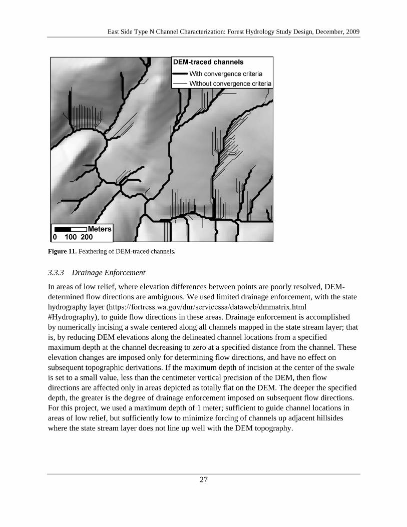
East Side Type N Channel Characterization: Forest Hydrology Study Design, December, 2009
27
Figure 11. Feathering of DEM-traced channels.
3.3.3 Drainage Enforcement
In areas of low relief, where elevation differences between points are poorly resolved, DEM-determined flow directions are ambiguous. We used limited drainage enforcement, with the state hydrography layer (https://fortress.wa.gov/dnr/servicessa/dataweb/dmmatrix.html #Hydrography), to guide flow directions in these areas. Drainage enforcement is accomplished by numerically incising a swale centered along all channels mapped in the state stream layer; that is, by reducing DEM elevations along the delineated channel locations from a specified maximum depth at the channel decreasing to zero at a specified distance from the channel. These elevation changes are imposed only for determining flow directions, and have no effect on subsequent topographic derivations. If the maximum depth of incision at the center of the swale is set to a small value, less than the centimeter vertical precision of the DEM, then flow directions are affected only in areas depicted as totally flat on the DEM. The deeper the specified depth, the greater is the degree of drainage enforcement imposed on subsequent flow directions. For this project, we used a maximum depth of 1 meter; sufficient to guide channel locations in areas of low relief, but sufficiently low to minimize forcing of channels up adjacent hillsides where the state stream layer does not line up well with the DEM topography.

East Side Type N Channel Characterization: Forest Hydrology Study Design, December, 2009
28
3.3.4 Delineation of Type N and Type F Channels
For this stage of the project, we use the current channel typing designated in the state hydrography. The Type-N to Type-F transition point identifies the outlet from which each Type-N (headwater) basin is delineated. Although the current stream typing contains many unverified and potentially incorrectly typed streams, it provides a sufficient means of identifying the population of Type N basins available for detailed mapping. As part of the field work for the implementation phase of the Forest Hydrology Study, the indicated F-to-N water-type breaks within the selected basins will be evaluated based on geomorphic criteria (e.g., channel gradient).
To use the state stream types, we needed to match the state hydrography with the DEM-traced channel locations. To do this, we applied a 50-meter buffer to all delineated Type F channels in the state stream layer. From each DEM-traced channel initiation point, we followed each DEM-traced channel downstream. From any point from which the traced channel extended greater than 50 meters through the Type-F buffer, all downstream reaches are designated as Type F channels and all upstream reaches as Type N channels.
3.4 Explanatory Variables
3.4.1 Conceptual Basis
A primary premise of this project is that the ecological functions and flow regime of Type-N streams are determined by a set of quantifiable controlling factors. Conceptually, we categorize these factors into four realms: geology, biology, hydrology, and climate. These are arbitrary distinctions, because multiple interactions, dependencies, and overlaps among these realms are inherent in ecological processes, but conceptually these divisions help us to sort through the complexities inherent in these systems. To characterize those factors that affect channel function listed in Table 1, we expect that information from each of these four realms is required. The focus of the Forest Hydrology Study is on the low-flow regime of channel discharge. At this stage of the channel-classification process, we have specific, spatially distributed information about certain aspects of climate and geology, including aspects of geomorphology. We lack information on hydrology and biology. Hydrologic data, in terms of low-flow regime (perennial, seasonal, discontinuous) from detailed field-based observations, and biologic data, in terms of forest type and riparian-vegetation cover from air-photo mapping and field observations, will be collected in the implementation phase of this project.
In this design phase of the project, based on current understanding of geologic, biologic, and climatic controls on channel hydrology, we must identify the factors that affect low-flow regime and determine to what extent these can be quantified with available data. To do this, we rely on a conceptual model of basin hydrology (see also Palmquist, 2005). Water from rainfall, snow melt, and glacial melt travels along surface and subsurface pathways (Anderson et al., 1997; Winter, 2007). The quantity of water is a function of climate, but is also influenced by the presence of forest cover. Loss of forest cover can reduce evapotranspiration and increase snow accumulation.
East Side Type N Channel Characterization: Forest Hydrology Study Design, December, 2009
29
Both processes increase available soil water and groundwater recharge, which can consequently increase the quantity of water available for stream flow (Moore and Wondzell, 2005). At a local extent, daytime transpiration from riparian vegetation can lower valley-floor water tables sufficient to affect stream discharge (Bren, 1997; Butler et al., 2007; Gooseff et al., 2008). Flow pathways are functions of surface topography (McGuire et al., 2005) and the spatial distribution of material properties that influence the rate and quantity of water carried by subsurface flow. These properties include the thickness and hydraulic conductivity of rock strata and soils. Bulk hydraulic conductivity is influenced by the extent and interconnectivity of pore space, the extent and orientation of fractures, and the presence of macropores, such as animal burrows. Small-scale features, such as impermeable layers of silt or till, or open fractures in rock, can have a large influence on groundwater flow paths and consequent Type-N channel hydrology.
Water routed through surface and subsurface flow paths to surface channels travels downstream through channel corridors both as surface discharge and as subsurface flow in the hyporheic zone. The quantity of water in hyporheic flow depends on the volume of pore space available in the channel substrate and valley fill; the greater the volume of valley-filling sediment, the greater is the volume of water that can be carried as hyporheic flow (Butturini et al., 2002). Presence of perennial or seasonal flow is thus influenced by the quantity of valley-filling sediment. Downstream changes in sediment volume result in downstream changes in surface and hyporheic discharge. Increases in sediment volume associated with debris fans, or widening valleys, or sediment accumulations upstream of wood jams, can cause streams to go dry as all flow is accommodated in the hyporheic zone (May and Lee, 2004). The volume of sediment depends on valley geometry and on sediment supply and transport processes.
This simple conceptual model of channel hydrology guides our choice of explanatory variables. We seek attributes that characterize the volume of water available, the topography, the substrate, and the volume of valley fill (for hyporheic flow). Of these, only topography can be directly resolved with available data (from the DEM); the others must be inferred from other measurements or interpolated (or extrapolated) from existing but spatially scattered observations (such as precipitation).
Many important controls on channel hydrology cannot be consistently resolved across eastern Washington FFR lands with available data. For example, available mapping of bedrock fracture density, orientation, and permeability is insufficient to characterize a potentially primary control on channel-head locations. However, fracture characteristics may be consistent within a particular rock type and to differ between rock types; a hypothesis supported by observations of differences in channel head locations and headwater flow regime between sandstone and basalt in western Washington (Jaeger et al., 2007). Within the constraints of available data, we seek attributes that relate directly or indirectly to physical controls on Type N channel hydrology. We do not know which of these attributes will prove useful for predicting flow regime, or what level of confidence to expect in these predictions. The building and testing of empirical models in the

East Side Type N Channel Characterization: Forest Hydrology Study Design, December, 2009
30
implementation phase of the Forest Hydrology Study will determine the degree to which available data can be used to predict low-flow regime.
This conceptual model of forest hydrology can also be used to form hypotheses concerning management influences on Type N channel hydrology. Timber harvest in Type N basins may reduce evapotranspiration, with subsequent increased low-flow discharge. Transient increases in base flow for periods up to a decade following loss of forest cover are well documented in the literature (Pike and Scherer, 2003). Timber harvest may also reduce the volume of in-channel wood (Ralph et al., 1994), with a subsequent reduction of in-channel sediment storage capacity and associated hyporheic flow. Both effects would tend to increase the length of channel with perennial flow. Forest roads may intercept surface and shallow subsurface flow, thereby increasing the rate at which precipitation is routed to stream channels and reducing the volume of water available for summer low flow. An important constraint imposed by available data, however, is our inability to resolve current forest cover, road locations, or channel and riparian-zone alterations (the state roads layer, for example, was deemed by SAGE as too inaccurate and inconsistent for use in this study). These data must, therefore, be collected through air-photo analysis and field surveys during the implementation phase of the Forest Hydrology Study. Management influences, as indicated by mapped forest cover and road networks, can then be evaluated in terms of effects on flow regime.
In collaboration with SAGE, we have identified a set of explanatory variables that are both indicative of the processes that control stream hydrology (and function) and that can be quantified with available GIS data. These variables can be divided between those that integrate spatially distributed quantities to characterize attributes of the contributing area to each 30-m channel reach, the source areas for water, sediment, and organic materials, and those attributes that average quantities over a reach length to characterize the channel environment locally.
3.4.2 Spatially Integrated Variables
• Drainage Area.
•
Calculated from DEM-derived flow directions using the D∞ algorithm (Tarboton, 1997). The drainage area to each DEM cell was delineated and spatially distributed attributes within the drainage area were summed to provide cumulative distributions and a variety of statistics (e.g., mean values).
Channel Length
•
. GIS-based channel flow paths precede from DEM point to point, based on the D8 flow-direction algorithm. Cumulative channel length was estimated as the summed length over all point-to-point channel segments.
Proportion of Basin Area in FFR Land. This variable is not related to any intrinsic property that affects channel processes, but rather was used to identify the set of Type N basins to include in this study.

East Side Type N Channel Characterization: Forest Hydrology Study Design, December, 2009
31
• Drainage Density
•
. Calculated as the cumulative channel length divided by the drainage area. Drainage density is proportional to average slope length and indicative of hydrological processes in the basin.
Mean Slope Gradient
•
. Surface gradient and aspect were calculated for every DEM cell by fitting a polynomial to the associated DEM point and its eight adjacent points (Zevenbergen and Thorne, 1987). The mean is calculated for all cells in the basin.
Mean Topographic Plan Curvature
•
. This value provides a measure of topographic dissection of the basin, and has been found to correlate with channel-head location (Heine et al., 2004).
Aspect
•
. Reported as the proportion of the basin area with northerly, easterly, southerly, and westerly aspects.
Mean Annual Precipitation
•
. Based on 1971-2000 precipitation data interpolated between climate stations with the PRISM model (Daly et al., 2008) at a horizontal resolution of about 800m. These data were downloaded from the PRISM website (http://www.prism.oregonstate.edu/) and are the most current data available. PRISM includes orographic and rain-shadow effects of topography in the interpolation scheme, so modeled values vary spatially. For this study, values were spatially averaged to obtain a mean value for each Type N basin.
Mean Annual Snow Depth
•
. Also estimated with the PRISM model and obtained from the Climate Source (http://www.climatesource.com). Values are based on climate data from 1961-1990 and are at a spatial resolution of approximately 2 km.
Storm Intensity
•
. These are from the NOAA Atlas 2 (Miller et al., 1973) (data available at http://www.nws.noaa.gov/oh/hdsc/noaaatlas2.htm) for 100-yr recurrence, 24-hr and 6-hr duration storms and 2-yr recurrence, 24-hr and 6-hr duration storms. Intensity is measured in terms of precipitation depth. The NOAA Atlas 2 was published in 1973; storm intensity maps included in the atlas are based on climate data spanning a temporal period from 1897 to 1970, depending on the period of operation of regional climate stations. Maps were originally drawn at a scale of 1:100,000 with an isopluvial contour interval of 0.5 inches. NOAA interpolated the isopluvial values and digitized over a grid of approximately 380-m spacing for distribution of the maps as digital GIS-readable grid files. For this project, grid values are averaged over each Type N basin area. (Although more recent data are available from individual weather stations, this is the only data set for storm intensity that has been interpolated to provide values across the entire study area that we are aware of).
Mean Annual Maximum and Minimum Temperature. From the PRISM website (http://www.prism.oregonstate.edu) based on data from the period 1971-2000. Data grids were at a spatial resolution of 800m.
East Side Type N Channel Characterization: Forest Hydrology Study Design, December, 2009
32
•
•
Proportion of Basin Area in Rain-on-Snow Zone. From the DNR rain-on-snow GIS map (https://fortress.wa.gov/dnr/servicessa/dataweb/dmmatrix.html #Climatology), based on mapping done at a scale of 1:250,000.
•
Rock Type. Lithologic units from the 1:100,000-scale geologic mapping(https://fortress.wa.gov/dnr/servicessa/dataweb/dmmatrix.html #Geology) were grouped into four general rock types: sedimentary, extrusive igneous, intrusive igneous and metamorphic, and Quaternary glacial, alluvial, colluvial, and mass-wasting deposits. The proportion of area in each rock type is reported for each Type N basin. Specific rock and geologic attributes, such as fracture density, fracture orientation, and saturated hydraulic conductivity, could potentially provide more specific information pertinent to groundwater flow that would better predict hydrologic regime than generic rock-type categories. However, such information is not consistently available across eastern Washington FFR lands.
Soil Properties.
•
The most consistent digital soils data are those provided by the SurveyGeographic (SSURGO) database (http://soildatamart.nrcs.usda.gov, also see Bandaragoda,attached report). These data cover most of eastern Washington FFR lands, but the data set isstill being assembled and not all attributes are available. We use soil depth and an estimate ofaverage saturated hydraulic conductivity (Bandaragoda, attached report), averaged over eachType N basin area.
Proportion in Wetlands.
Two additional spatially integrated variables will be calculated from data collected from digitized mapping on aerial photographs during the implementation phase:
Wetland locations were taken from the fpwetlands GIS data layer (https://fortress.wa.gov/dnr/servicessa/dataweb/dmmatrix.html #Forest%20Practices).
• Proportion of area in forest cover.
•
The proportion of contributing area with forest cover will be used to assess relationships between flow regime for each reach and the extent of forest cover in the contributing area to the reach. The literature provides no quantitative guidance to relate extent of forest cover to base flow. To provide data to seek such relationships, each mapped Type-N basin will be mapped in terms of forested and unforested areas, with forested areas divided into four canopy-cover classes. Canopy cover is related to stand age and associated hydrologic effects and can be estimated and mapped into distinct classes on aerial photographs. The proportion of contributing area in each cover class (unforested, 0-25%, 25-50%, 50-75%, and75-100% canopy cover) will be calculated for each reach.
Road density. Road networks mapped from the orthophotos will be used to calculate road density for the contributing area to each reach.

East Side Type N Channel Characterization: Forest Hydrology Study Design, December, 2009
33
3.4.3 Reach Based Variables
• Channel Gradient. Channel gradient was estimated for each DEM channel cell by fitting a 2nd
•
-order polynomial to all channel cell elevations over a centered window of specified length. The length of the window varies with channel gradient, using a longer distance (up to 1000 meters) for low-gradient channels (< 1%) and varying linearly to shorter distances (300 meters) for high-gradient channels (> 20%). This algorithm works well and generally matches channel gradients determined by measuring channel length along blue-line channels between contour lines on the 1:24,000-scale maps that the DEMs were derived from. The degree to which DEM-determined gradients match field-measured gradients tends to vary from region to region (Neeson et al., 2008). The variability may reflect differences in channel topography not resolved in the topographic maps. For example, if channel relief occurs primarily in short, steep steps interspersed with longer, lower-gradient reaches, the field-measured gradient is likely to be less than the DEM measured gradient because the two methods are measuring gradient over different length scales.
Valley width
•
. Valley width was estimated by summing the area draining to each reach within a certain elevation of the channel and dividing this area by reach length. Elevation differences are measured along flow lines. We use an elevation difference of 5 bank-full channel depths, with bank-full depth based on regional regressions to drainage area (Castro and Jackson, 2001). This regression will be refined as field data become available.
Downslope Change in Channel Gradient and Valley Width
•
. Average gradient and valley width were calculated for every reach; reach-to-reach changes in gradient and valley width can reflect changes in sediment transport process (e.g., debris flow to fluvial) and indicate where reductions in transport potential, and consequent sediment deposition, are likely to occur. Downstream reductions in gradient and increases in valley width are indicative of depositional zones and identify areas with greater alluvial fill.
Flow Distance to Drainage Divide
•
. In the pilot study (Palmquist, 2005), distance to the drainage divide (based on a line traced perpendicular to contour lines on 1:24,000-scale USGS topographic maps from the up-slope-most point of perennial flow to the divide) proved a relatively good indicator of channel-head location, and distance from the channel head proved a potential candidate for identifying potential Ns/Np transition points. There are multiple flow paths from which to determine distance to the divide; as a starting point we calculated the minimum, maximum, and average flow distance to the divide for the upstream point of each reach.
Travel Time from Drainage Divide. Slope gradient is also an important control on surface and subsurface flow rates. For example, for shallow subsurface flow roughly parallel to the ground surface, discharge q is calculated as q = TS sinθ, where TS is soil transmissivity (saturated hydraulic conductivity Ksat integrated over soil depth) and θ is ground-surface slope (measured from horizontal). This gives a Darcy velocity proportional to 1/sinθ, a travel

East Side Type N Channel Characterization: Forest Hydrology Study Design, December, 2009
34
time proportional to L/sinθ, where L is the travel distance. We calculate two relative indices of travel time from the divide:
T = Σ(L i/sinθ i(1) )
where Li is the slope distance through the ith cell, qi is the slope of the ith
cell, and the sum is over all DEM cells along the travel path, and
TR = LR/sinθ (2) R
where LR is the straight-line distance from the divide to the stream reach (i.e., LR = (X2 + Y2)1/2 where X is the horizontal distance and Y is the elevation difference) and θR is the slope of that straight line (i.e., sinθR = Y/LR
• Riparian stand type, based on aerial photograph interpretation (using the four canopy cover classes specified above) and on field surveys (required observations are specified in Section 4.3.2)
).
The spatially integrated variables are calculated for every delineated Type N basin. To preclude inclusion of very small DEM-delineated basins, which may not actually contain any channels, we preclude basins less than 100 hectares (247 acres). To include only basins containing FFR lands, we remove those with less than 50% of area in FFR lands and less than 75% forested (based on CMER-provided land cover classification). The remaining basins compose the population of Type N channels to be classified, that is, the sample frame. Note that the SAMPLE software allows a different set of threshold criteria to be used to define the sample frame; for example, a different minimum proportion in FFR lands can be specified. We now select a subset of these basins for detailed analysis.
3.5 10-m DEMs versus LiDAR DEMs
This discussion is prompted by review comments to an earlier draft of this report. Several reviewers asked if the 10-m DEMs are adequate to accomplish the objectives of the study, particularly given the perceived poor accuracy of the habitat model (Conrad et al., 2003) for site-level evaluations (Cupp, 2005).
3.5.1 Limitations and advantages of the 10-m DEMs.
These digital elevation models (DEMs) were created by the US Geological Survey using interpolation of elevations from contour lines on the 1:24,000-scale USGS topographic maps (see http://rockyweb.cr.usgs.gov/nmpstds/demstds.html). These data can resolve no more than what is resolved on the original maps, which do not resolve many headwater streams or small drainage divides. Hence, stream networks derived from these data will miss potential channel
East Side Type N Channel Characterization: Forest Hydrology Study Design, December, 2009
35
courses and will in some cases indicate channels where none exist (Cupp, 2005; Heine et al., 2004; Mouton, 2005). Moreover, the ability of these maps to resolve headwater streams can vary from quadrangle to quadrangle (Clarke et al., 2008). Contour lines were originally traced from stereo photo pairs. Resolution of fine-scale topographic features differs between forested and unforested (e.g., recently clearcut or burned) areas on the photos. Likewise, different photo-interpreters tended to differ in the degree to which they traced fine-scale topographic crenulations, which can result in substantial differences in the spatial density of headwater channels traced from different (even adjacent) quadrangles.
Uncertainties associated with limitations on resolution of topographic features in these data can be quantified in terms of observed differences obtained from different measurement techniques, e.g., DEM-traced channel locations versus field GPS points (Colson et al., 2006), or DEM-traced channel length versus channel lengths traced on digital orthophotos (Heine et al., 2004). In the context of this study, these limitations will affect the level of certainty in identification of channel locations and channel hydrologic regime. For individual survey reaches, the magnitude of these uncertainties will vary with position on the landscape and will be substantial. Colson et al. (2006), for example, found that blue-line streams on the USGS topographic maps for headwater streams in North Carolina were within 10-m of field-surveyed stream locations in only 5 – 17% of the observed cases. For our use, however, precise location of stream channels may be of lesser importance than precise determination of channel length and associated landforms. Heine et al. (2004), for example, found that stream lengths traced from the USGS 10-m DEMs in central Kansas (counting both missed streams and traced streams that didn't actually exist) were 87% accurate.
This difference in estimated accuracy between these two studies illustrates the scale dependence of measurement accuracy. If the goal is to obtain high (e.g., 90% correct predictions) at an individual reach scale, it cannot be done with these data; if the goal is to correctly predict the length of different stream types within a basin, we have the potential for high accuracy. We think that such predictions can be used to accomplish the objectives of the Forest Hydrology Study. This is particularly true if one of the objectives is to make predictions of flow regime for FFR lands over all of eastern Washington State, because there are no other topographic data at this regional extent.
The study is designed to use the 10-m DEMs to estimate a variety of topographic attributes that we think might affect flow regime. We propose a list of attributes that is substantially larger than that examined in any of the previous studies that we are aware of (e.g., Heine et al., 2004; McCleary and Hassan, 2008; Palmquist, 2005). This list was based on both the physical attributes that were identified in numerous SAGE meetings as potentially important controls on flow regime and on the availability of consistent and usable data over the entire study area. For some of these (e.g., flow length, subsurface flow travel time), we developed new algorithms and implement them in computer code. We don't know how or if this expanded list of explanatory variables will improve predictive power, but because a greater number of potential controlling

East Side Type N Channel Characterization: Forest Hydrology Study Design, December, 2009
36
factors are represented by variables in this list (as opposed to that used in Palmquist, 2005, for example), we expect to obtain better predictive power than found in previous studies.
It is also important to note that the dependent variables to be predicted by this study (section 1.3.1) include attributes different than those addressed in previous studies. At the finest grain of analysis, we suggest that logistic regression be used to predict probable flow regime for every DEM-traced reach. This grain of analysis is similar to that of previous studies (Conrad et al., 2003; Fransen et al., 2006; Palmquist, 2005) and resulting model predictions can be tested with field observations (e.g., Cupp, 2005; Terrapin Environmental, 2004). However, once these reach-scale models are assembled, they can then be aggregated to predict coarser-grained attributes that provide other types of information and can also be evaluated against field observations. For example, the models can be used to predict the upstream length of perennial stream flow contiguous from the Type F-to-N transition. These types of predictions will exhibit higher levels of confidence than the reach-based predictions; such types of predictions have not been evaluated in previous studies.
3.5.2 Limitations and advantages of LiDAR-derived DEMs
LiDAR data provide digital elevation data of much higher resolution (e.g., 1-m horizontal spacing) and vertical accuracy than the currently available 10-m DEMs (Hodgson and Bresnahan, 2004), and channel networks derived from these data are considerably more accurate than those obtained from the 10-m DEMs (Mouton, 2005; Murphy et al., 2008). Data accuracy is variable, depending on ground surface slope, vegetation cover, and the altitude of the instrument during data acquisition (Hodgson et al., 2005), but is still consistently better than that currently available. Regression models based on comparison of photo-mapped and field surveyed measurements to topographic attributes obtained from LiDAR DEMs would undoubtedly provide greater confidence than regressions to topographic attributes derived from the USGS 10-m DEMs. LiDAR data still contain errors and uncertainties, but they are smaller than those contained in the 10-m DEMs. The primary obstacle to use of LiDAR is lack of data. The state currently has no program for LiDAR data collection in eastern Washington (Jeff Grizzel, personal communication).
Because characterization of flow regime over all FFR lands in Eastern Washington is one of the study objectives, the study design is based on currently available data. However, in comparison to field surveys, LiDAR may be a cost-effective method of high-resolution data collection. This would depend on the amount of information that could be obtained from LiDAR in conditions found in the study area. In part, this would depend on the data resolution provided by the LiDAR contractor – which depends on the altitude of the instrument and the time of year data are collected. Higher data resolution will impose greater costs. If LiDAR can provide highly accurate estimates of topographic attributes that are strongly correlated with flow regime, then LiDAR could supplement or even replace field surveys for some portion of the sample basins, which could result in cost reductions. LiDAR would also provide information on forest stand

East Side Type N Channel Characterization: Forest Hydrology Study Design, December, 2009
37
characteristics. Nevertheless, field surveys over a representative set of sample basins would first be required to evaluate the LiDAR data.
3.6 Stratified Random Sample
3.6.1 Sample Selection
FFR lands across eastern Washington span a large range of geomorphic, geologic, and climatic conditions. GIS delineation and characterization of the Type N basins traced from the 10-m DEMs provide a measure of this range. Each delineated basin is a candidate for detailed mapping and field surveys of the Type N channels within it, from which statistics describing the conditions associated with different flow regimes will be obtained.
We provide two computer programs based on the concepts and equations presented in this section: SAMPLE, used to define the sample frame and select an initial stratified, random sample of basins, and RESAMPLE, used to replace or add basins to an existing set of sample basins to maintain the distribution of characteristics among strata as that in the initial sample. SAMPLE will be used during the implementation phase of the project to select specific basins for photo mapping and field surveys. We expect that some of the basins in the initial survey will prove inaccessible or inappropriate, or that the initial sample size may prove too small, so RESAMPLE provides capabilities to replace basins or add to the initial sample.
To minimize bias in the selected basins, we use a random sample stratified by two variables: mean annual precipitation, as suggested by Palmquist (2005), and rock type, based on work by Jaeger et al. (2007). We expect that these two variables impose the primary controls on flow regime (from our list of candidate explanatory variables). All climatic variables correlate with mean annual precipitation (look ahead to Figure 15).
Stratification serves two purposes (Cochran, 1977).
1) To ensure that all subpopulations, even those with relatively few basins, are included in our sample. For example, the number of basins lying predominately in sedimentary rocks is relatively small compared to the number in other rock types (Figure 3). We want to make sure that the randomly selected basins include channels in sedimentary rock types.
2) The relationships between explanatory variables and flow regime may vary among the sampling strata. For example, we may find that the average drainage area to first perennial flow tends to differ between basins in sedimentary and volcanic rock types (e.g., Jaeger et al., 2007). We would therefore want to analyze these subpopulations separately.
There are three options for setting the number of samples to include in each strata:
1) Proportional to the size of the stratum; if strata are divided equally across the range of variable values, samples are distributed equally across all strata. We assume equally sized strata for the remainder of this discussion.
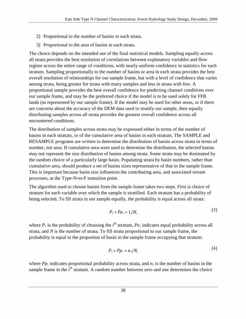
East Side Type N Channel Characterization: Forest Hydrology Study Design, December, 2009
38
2) Proportional to the number of basins in each strata.
3) Proportional to the area of basins in each strata.
The choice depends on the intended use of the final statistical models. Sampling equally across all strata provides the best resolution of correlations between explanatory variables and flow regime across the entire range of conditions, with nearly uniform confidence in statistics for each stratum. Sampling proportionally to the number of basins or area in each strata provides the best overall resolution of relationships for our sample frame, but with a level of confidence that varies among strata, being greater for strata with many samples and less in strata with few. A proportional sample provides the best overall confidence for predicting channel conditions over our sample frame, and may be the preferred choice if the model is to be used solely for FFR lands (as represented by our sample frame). If the model may be used for other areas, or if there are concerns about the accuracy of the DEM data used to stratify our sample, then equally distributing samples across all strata provides the greatest overall confidence across all encountered conditions.
The distribution of samples across strata may be expressed either in terms of the number of basins in each stratum, or of the cumulative area of basins in each stratum. The SAMPLE and RESAMPLE programs are written to determine the distribution of basins across strata in terms of number, not area. If cumulative area were used to determine the distribution, the selected basins may not represent the size distribution of basins among strata. Some strata may be dominated by the random choice of a particularly large basin. Populating strata by basin numbers, rather than cumulative area, should produce a set of basins sizes representative of that in the sample frame. This is important because basin size influences the contributing area, and associated stream processes, at the Type-N-to-F transition point.
The algorithm used to choose basins from the sample frame takes two steps. First is choice of stratum for each variable over which the sample is stratified. Each stratum has a probability of being selected. To fill strata in our sample equally, the probability is equal across all strata:
P i = Pe i(3) = 1/N,
where Pi is the probability of choosing the ith stratum, Pei
indicates equal probability across all strata, and N is the number of strata. To fill strata proportional to our sample frame, the probability is equal to the proportion of basin in the sample frame occupying that stratum:
P i = Pp i = n i(4) /N,
where Ppi indicates proportional probability across strata, and ni is the number of basins in the sample frame in the ith stratum. A random number between zero and one determines the choice
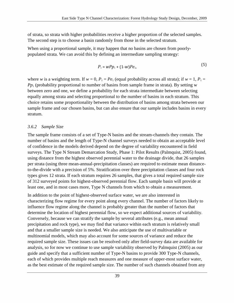
East Side Type N Channel Characterization: Forest Hydrology Study Design, December, 2009
39
of strata, so strata with higher probabilities receive a higher proportion of the selected samples. The second step is to choose a basin randomly from those in the selected stratum.
When using a proportional sample, it may happen that no basins are chosen from poorly-populated strata. We can avoid this by defining an intermediate sampling strategy:
P i = wPp i + (1-w)Pe i(5) ,
where w is a weighting term. If w = 0, Pi = Pei (equal probability across all strata); if w = 1, Pi = Ppi
3.6.2 Sample Size
(probability proportional to number of basins from sample frame in strata). By setting w between zero and one, we define a probability for each strata intermediate between selecting equally among strata and selecting proportional to the number of basins in each stratum. This choice retains some proportionality between the distribution of basins among strata between our sample frame and our chosen basins, but can also ensure that our sample includes basins in every stratum.
The sample frame consists of a set of Type-N basins and the stream-channels they contain. The number of basins and the length of Type-N channel surveys needed to obtain an acceptable level of confidence in the models derived depend on the degree of variability encountered in field surveys. The Type N Stream Demarcation Study, Phase 1: Pilot Results (Palmquist, 2005) found, using distance from the highest observed perennial water to the drainage divide, that 26 samples per strata (using three mean-annual-precipitation classes) are required to estimate mean distance-to-the-divide with a precision of 5%. Stratification over three precipitation classes and four rock types gives 12 strata. If each stratum requires 26 samples, that gives a total required sample size of 312 surveyed points for highest-observed perennial flow. Each sample basin will provide at least one, and in most cases more, Type N channels from which to obtain a measurement.
In addition to the point of highest-observed surface water, we are also interested in characterizing flow regime for every point along every channel. The number of factors likely to influence flow regime along the channel is probably greater than the number of factors that determine the location of highest perennial flow, so we expect additional sources of variability. Conversely, because we can stratify the sample by several attributes (e.g., mean annual precipitation and rock type), we may find that variance within each stratum is relatively small and that a smaller sample size is needed. We also anticipate the use of multivariable or multinomial models, which may also account for some sources of variance and reduce the required sample size. These issues can be resolved only after field-survey data are available for analysis, so for now we continue to use sample variability observed by Palmquist (2005) as our guide and specify that a sufficient number of Type-N basins to provide 300 Type-N channels, each of which provides multiple reach measures and one measure of upper-most surface water, as the best estimate of the required sample size. The number of such channels obtained from any
East Side Type N Channel Characterization: Forest Hydrology Study Design, December, 2009
40
random selection of basins is included in the output from the SAMPLE and RESAMPLE programs.
3.7 Temporal Characteristics
The first objective for the Forest Hydrology Study is to "Determine the spatial and temporal characteristics of surface water discharge in Type N streams across eastern Washington FFR lands." We have described methods for examining spatial characteristics, but not temporal characteristics. Two time scales are of interest: within-year variations in the extent of surface discharge and year-to-year variations in the extent of perennial flow.
To obtain a sample of sufficient size for statistically significant inferences, repeated field surveys provide the most cost-effective strategy: we expect the costs involved to install and maintain sufficient in-stream instrumentation to monitor surface flow across eastern Washington FFR lands would be prohibitive. Observations of seasonal variations require repeated field observations over the course of a single summer; observations of year-to-year variations require repeated observations in multiple years. Repeat surveys need not record all the measurements required for the initial survey, but rather may focus solely on observations of surface discharge.
We expect that spatially distributed factors exert important controls on temporal characteristics. For example, Jeager et al. (2007) found consistent differences in the seasonal-migration distance for surface-flow initiation between streams underlain by sandstone and basalt. Design of a sampling protocol to assess temporal variability would therefore benefit from prior analysis of spatial controls on stream base-flow regime. The initial sample and analysis will identify appropriate strata for subsequent resampling to resolve temporal variability. For this reason, after discussion with SAGE, it was decided to postpone design of the resurvey sampling scheme to during and after data collection and analysis during the implementation phase of this project.
3.8 GIS Analysis Results
3.8.1 Delineated Type N Basins
Analyses were performed for all portions of eastern Washington containing FFR lands. Over 120,000 Type N basins were delineated using the protocol described above. To define the sampling frame, this population can be filtered by basin area, traced channel length, proportion of area in forested lands, and proportion of area in FFR lands. These are included as inputs to the SAMPLE computer program written for this project. The total population of delineated basins and an example sample frame are shown in Figure 12. The frequency distribution of basin area and traced channel length for all Type N basins with greater-than-zero area in FFR lands is shown in Figure 13. This reflects the total population from which the sample frame may be defined.

East Side Type N Channel Characterization: Forest Hydrology Study Design, December, 2009
41
Figure 12. Type N basins for FFR lands in eastern Washington. For this example, threshold values used to define the sample frame were: area > 0.1 km2, channel length > 500m, proportion FFR lands > 20%, sample size = 300.
We have no a priori basis for setting the threshold values of basin area, channel length, proportion of forested land, and proportion of FFR lands used to define the sample frame. Figure 13 shows the cumulative distributions for basin area and channel length for Type N basins containing any FFR lands. (Scatter plot C in Figure 13 also shows that these two variables are highly correlated, so the threshold is effectively set by either of the two). We want to ensure that steep, debris-flow-prone Type N channels are included in our sample frame. Scatter plot D in Figure 13 shows that steep basins are well distributed over all total basin channel lengths (and thereby, basin areas), so filtering small basins is unlikely to bias our sample to non-debris-flow-prone basins, and can allow the field effort to focus more efficiently on larger basins. The area threshold used for examples in this report, 0.1 square kilometers (247 acres), extends well into the realm of debris-flow-incised channels (Stock and Dietrich, 2003). Another concern with small delineated basins is that, if our channel delineation criteria tend to overestimate channel extent and trace channels where none actually exist, many of the small DEM-traced basins may actually contain no channels.
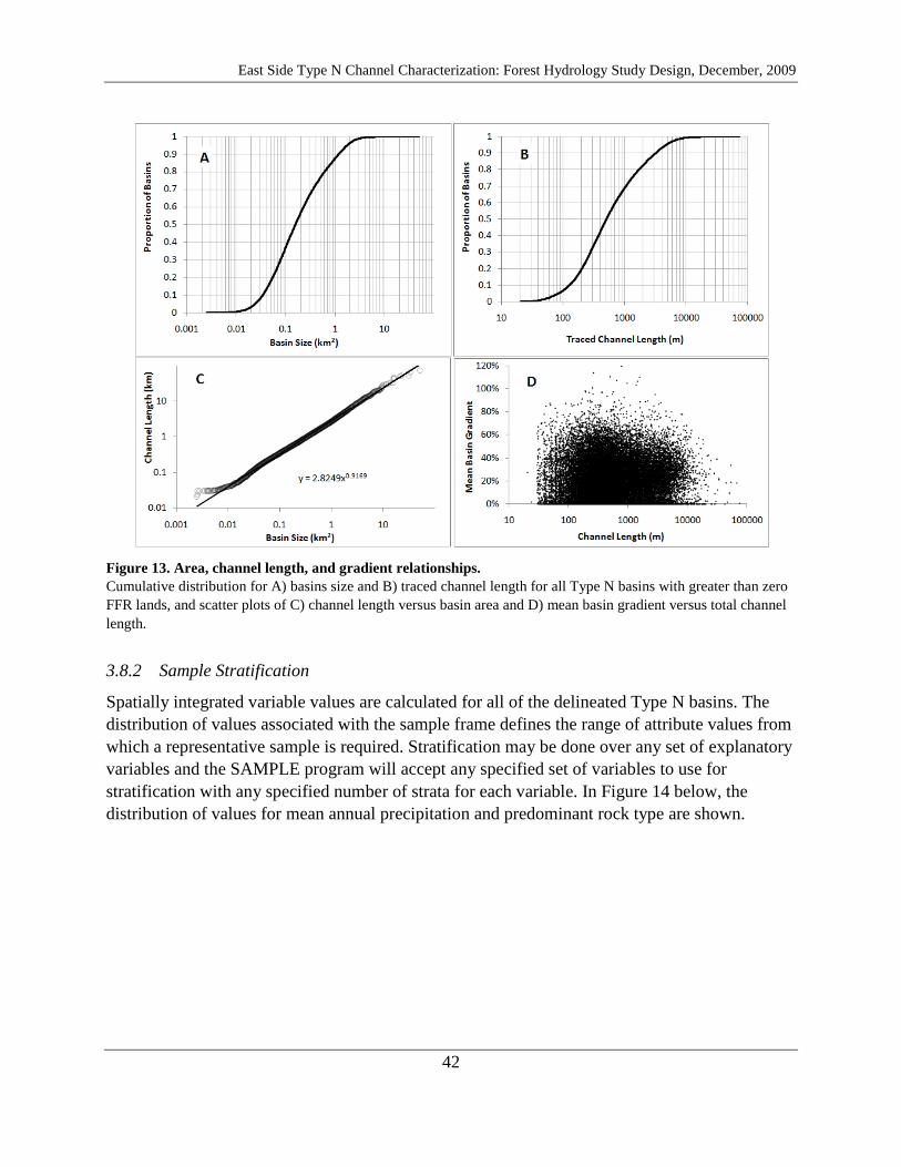
East Side Type N Channel Characterization: Forest Hydrology Study Design, December, 2009
42
Figure 13. Area, channel length, and gradient relationships. Cumulative distribution for A) basins size and B) traced channel length for all Type N basins with greater than zero FFR lands, and scatter plots of C) channel length versus basin area and D) mean basin gradient versus total channel length.
3.8.2 Sample Stratification
Spatially integrated variable values are calculated for all of the delineated Type N basins. The distribution of values associated with the sample frame defines the range of attribute values from which a representative sample is required. Stratification may be done over any set of explanatory variables and the SAMPLE program will accept any specified set of variables to use for stratification with any specified number of strata for each variable. In Figure 14 below, the distribution of values for mean annual precipitation and predominant rock type are shown.
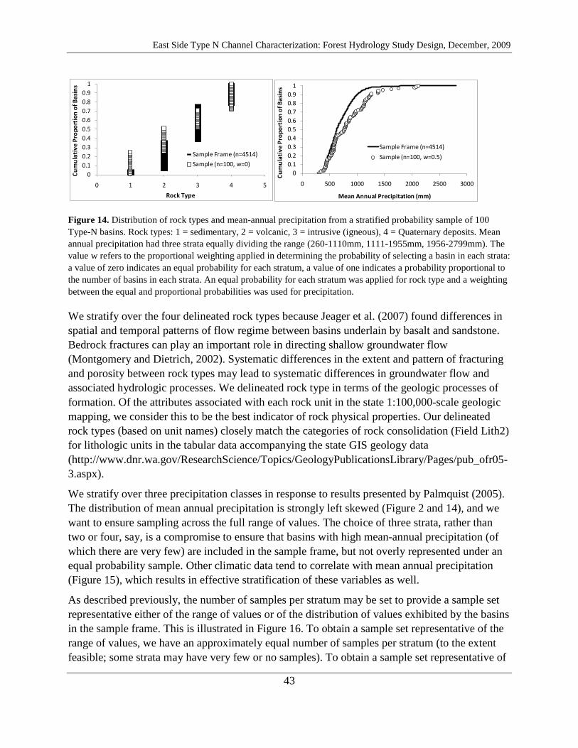
East Side Type N Channel Characterization: Forest Hydrology Study Design, December, 2009
43
Figure 14. Distribution of rock types and mean-annual precipitation from a stratified probability sample of 100 Type-N basins. Rock types: 1 = sedimentary, 2 = volcanic, 3 = intrusive (igneous), 4 = Quaternary deposits. Mean annual precipitation had three strata equally dividing the range (260-1110mm, 1111-1955mm, 1956-2799mm). The value w refers to the proportional weighting applied in determining the probability of selecting a basin in each strata: a value of zero indicates an equal probability for each stratum, a value of one indicates a probability proportional to the number of basins in each strata. An equal probability for each stratum was applied for rock type and a weighting between the equal and proportional probabilities was used for precipitation.
We stratify over the four delineated rock types because Jeager et al. (2007) found differences in spatial and temporal patterns of flow regime between basins underlain by basalt and sandstone. Bedrock fractures can play an important role in directing shallow groundwater flow (Montgomery and Dietrich, 2002). Systematic differences in the extent and pattern of fracturing and porosity between rock types may lead to systematic differences in groundwater flow and associated hydrologic processes. We delineated rock type in terms of the geologic processes of formation. Of the attributes associated with each rock unit in the state 1:100,000-scale geologic mapping, we consider this to be the best indicator of rock physical properties. Our delineated rock types (based on unit names) closely match the categories of rock consolidation (Field Lith2) for lithologic units in the tabular data accompanying the state GIS geology data (http://www.dnr.wa.gov/ResearchScience/Topics/GeologyPublicationsLibrary/Pages/pub_ofr05-3.aspx).
We stratify over three precipitation classes in response to results presented by Palmquist (2005). The distribution of mean annual precipitation is strongly left skewed (Figure 2 and 14), and we want to ensure sampling across the full range of values. The choice of three strata, rather than two or four, say, is a compromise to ensure that basins with high mean-annual precipitation (of which there are very few) are included in the sample frame, but not overly represented under an equal probability sample. Other climatic data tend to correlate with mean annual precipitation (Figure 15), which results in effective stratification of these variables as well.
As described previously, the number of samples per stratum may be set to provide a sample set representative either of the range of values or of the distribution of values exhibited by the basins in the sample frame. This is illustrated in Figure 16. To obtain a sample set representative of the range of values, we have an approximately equal number of samples per stratum (to the extent feasible; some strata may have very few or no samples). To obtain a sample set representative of
00.10.20.30.40.50.60.70.80.9
1
0 1 2 3 4 5
Cum
ulat
ive
Prop
orti
on o
f Bas
ins
Rock Type
Sample Frame (n=4514)
Sample (n=100, w=0)0
0.10.20.30.40.50.60.70.80.9
1
0 500 1000 1500 2000 2500 3000
Cum
ulat
ive
Prop
orti
on o
f Bas
ins
Mean Annual Precipitation (mm)
Sample Frame (n=4514)
Sample (n=100, w=0.5)

East Side Type N Channel Characterization: Forest Hydrology Study Design, December, 2009
44
the distribution of values found in the sample frame, we have the number of samples per stratum proportional to the number of basins from the sample frame in that stratum.
Members of SAGE have expressed concern that the sample frame, if it is limited to FFR lands (which include less than one third of forested lands in eastern Washington, Figure 1), is not representative of all eastern Washington forested lands. If the sample frame is limited to basins containing FFR lands, one approach for addressing this concern is to populate all strata equally in sample selection, rather than proportional to the number of basins from the sample frame in each strata, which will provide the most widely applicable model. However, because there are very few basins with high precipitation values (Figure 14), this will also result in poor geographical distribution of the sample basins. As a compromise, we use equally populated strata for rock type and weighted probability, Equation (3) with w = 0.5, for mean annual precipitation, as used in Figure 14.
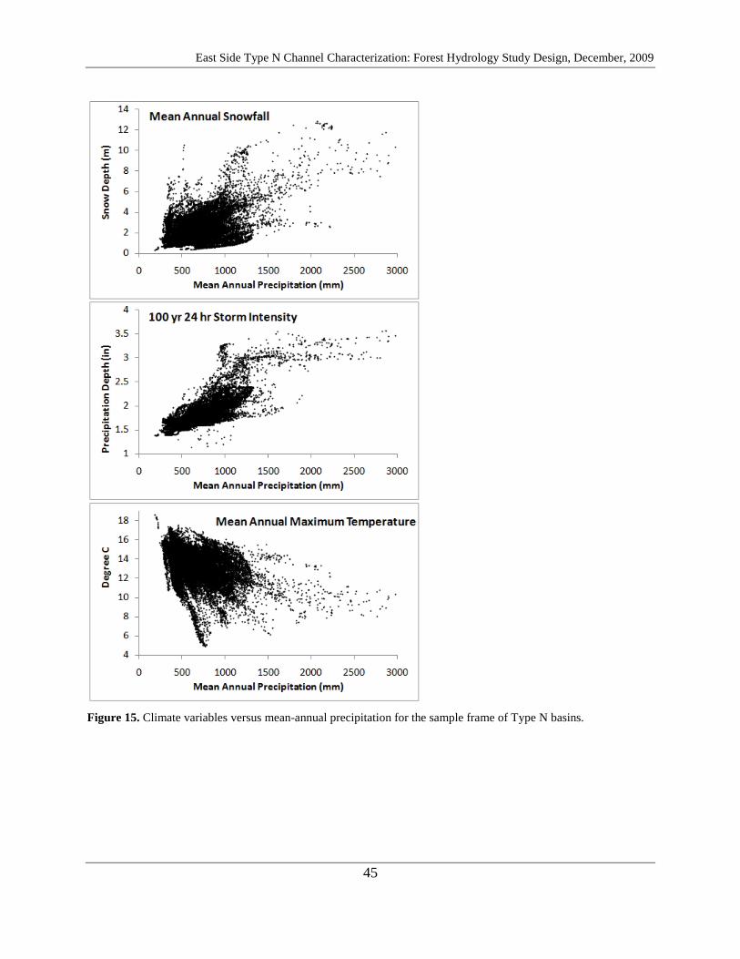
East Side Type N Channel Characterization: Forest Hydrology Study Design, December, 2009
45
Figure 15. Climate variables versus mean-annual precipitation for the sample frame of Type N basins.
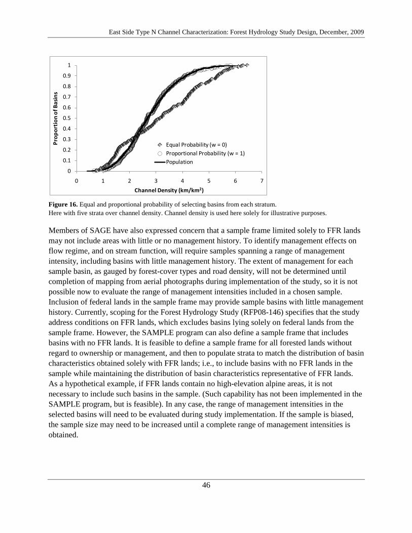
East Side Type N Channel Characterization: Forest Hydrology Study Design, December, 2009
46
Figure 16. Equal and proportional probability of selecting basins from each stratum. Here with five strata over channel density. Channel density is used here solely for illustrative purposes.
Members of SAGE have also expressed concern that a sample frame limited solely to FFR lands may not include areas with little or no management history. To identify management effects on flow regime, and on stream function, will require samples spanning a range of management intensity, including basins with little management history. The extent of management for each sample basin, as gauged by forest-cover types and road density, will not be determined until completion of mapping from aerial photographs during implementation of the study, so it is not possible now to evaluate the range of management intensities included in a chosen sample. Inclusion of federal lands in the sample frame may provide sample basins with little management history. Currently, scoping for the Forest Hydrology Study (RFP08-146) specifies that the study address conditions on FFR lands, which excludes basins lying solely on federal lands from the sample frame. However, the SAMPLE program can also define a sample frame that includes basins with no FFR lands. It is feasible to define a sample frame for all forested lands without regard to ownership or management, and then to populate strata to match the distribution of basin characteristics obtained solely with FFR lands; i.e., to include basins with no FFR lands in the sample while maintaining the distribution of basin characteristics representative of FFR lands. As a hypothetical example, if FFR lands contain no high-elevation alpine areas, it is not necessary to include such basins in the sample. (Such capability has not been implemented in the SAMPLE program, but is feasible). In any case, the range of management intensities in the selected basins will need to be evaluated during study implementation. If the sample is biased, the sample size may need to be increased until a complete range of management intensities is obtained.
0
0.1
0.2
0.3
0.4
0.5
0.6
0.7
0.8
0.9
1
0 1 2 3 4 5 6 7
Prop
orti
on o
f Bas
ins
Channel Density (km/km2)
Equal Probability (w = 0)Proportional Probability (w = 1)Population
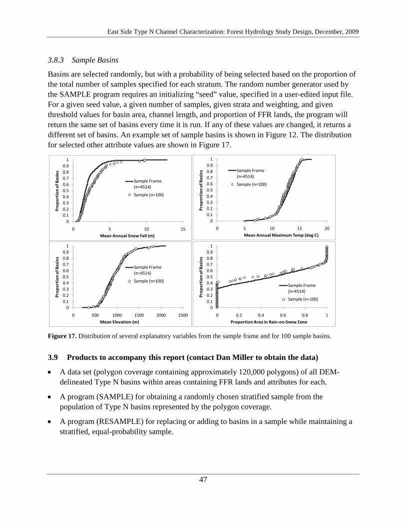
East Side Type N Channel Characterization: Forest Hydrology Study Design, December, 2009
47
3.8.3 Sample Basins
Basins are selected randomly, but with a probability of being selected based on the proportion of the total number of samples specified for each stratum. The random number generator used by the SAMPLE program requires an initializing “seed” value, specified in a user-edited input file. For a given seed value, a given number of samples, given strata and weighting, and given threshold values for basin area, channel length, and proportion of FFR lands, the program will return the same set of basins every time it is run. If any of these values are changed, it returns a different set of basins. An example set of sample basins is shown in Figure 12. The distribution for selected other attribute values are shown in Figure 17.
Figure 17. Distribution of several explanatory variables from the sample frame and for 100 sample basins.
3.9 Products to accompany this report (contact Dan Miller to obtain the data)
• A data set (polygon coverage containing approximately 120,000 polygons) of all DEM-delineated Type N basins within areas containing FFR lands and attributes for each.
• A program (SAMPLE) for obtaining a randomly chosen stratified sample from the population of Type N basins represented by the polygon coverage.
• A program (RESAMPLE) for replacing or adding to basins in a sample while maintaining a stratified, equal-probability sample.
00.10.20.30.40.50.60.70.80.9
1
0 5 10 15
Prop
orti
on o
f Bas
ins
Mean Annual Snow Fall (m)
Sample Frame (n=4514)
Sample (n=100)
00.10.20.30.40.50.60.70.80.9
1
0 5 10 15 20
Prop
orti
on o
f Bas
ins
Mean Annual Maximum Temp (deg C)
Sample Frame (n=4514)
Sample (n=100)
00.10.20.30.40.50.60.70.80.9
1
0 500 1000 1500 2000 2500
Prop
orti
on o
f Bas
ins
Mean Elevation (m)
Sample Frame (n=4514)
Sample (n=100)
00.10.20.30.40.50.60.70.80.9
1
0 0.2 0.4 0.6 0.8 1
Prop
orti
on o
f Bas
ins
Proportion Area in Rain-on-Snow Zone
Sample Frame (n=4514)
Sample (n=100)

East Side Type N Channel Characterization: Forest Hydrology Study Design, December, 2009
48
• A line coverage for DEM traced channels, with reaches defined and attribute values assigned. These attributes are intended to serve as explanatory variables in models to be calibrated and evaluated with field data.
4 REQUIREMENTS FOR PROJECT IMPLEMENTATION
4.1 Use of Products from the Forest Hydrology Study
How will data and models from the Forest Hydrology Study ultimately be used? This question should guide decisions in devising methods of data collection, data analysis, and model design. These uses, for example, determine the resolution, precision, and accuracy that will be required. Specific uses for study results are not specified in RFP08-146; however the goal of the project (from Section 1.1) provides guidance:
"The eastern Washington Type N stream research program, including this study, means to improve our knowledge of the character, distribution, and function of these streams in order to help stakeholders agree on appropriate forest practice rules for these stream channels."
What level of resolution, precision, and accuracy are required to "improve knowledge" to "help stakeholders agree on appropriate forest practice rules"? Experience suggests that no level is sufficient to get all stakeholders to agree; this is a consequence of dealing with a stochastic natural system, which exhibits inherent uncertainty that no level of accuracy and precision can remove, and with diverse stakeholders with sometimes opposing goals in managing this system. For such a case, it is useful to provide data and models that predict attributes of the system (e.g., flow regime) and that describe the nature and level of uncertainty in this system. The attributes predicted and the nature of the associated uncertainty depends on the application. We list below four examples.
On-the-ground, site evaluations for determination of stream type and function. Consistent with the scope defined for the Forest Hydrology study, we do not seek a detailed list of observations required to unambiguously define flow regime at the site scale. Rather, we have sought observations that can be collected quickly and over large extents to provide a coarse-grained picture of surface-water discharge characteristics across the geographic extent of eastern Washington FFR lands. Applicable, detailed, site-specific methods have been developed in other studies (Fritz et al., 2006; Topping et al., 2009).
Even if the current state of flow can be unambiguously determined during a site visit, however, uncertainty about temporal variability and stream function will persist. The eastern Washington research program should help to reduce and characterize this uncertainty, but several aspects of the natural system limit the degree to which field interpretations can increase confidence:
East Side Type N Channel Characterization: Forest Hydrology Study Design, December, 2009
49
a. Factors controlling processes of water, sediment, and organic material supply and transport are distributed spatially and temporally and many of these controlling factors are not readily apparent at the scale of observation provided by field observations.
b. There are numerous confounding factors, so that even high-resolution, highly accurate field measurements may be inadequate to accurately assess the full suite of functions provided by the stream or to anticipate the effects of management actions, or natural disturbances, on the associated processes.
c. The effects of management actions may depend on the specific sequence of weather events that occur in the subsequent years.
d. For any specific site, the supply and transport of water, sediment, and organic material from headwater areas to fish-bearing streams occurs over a potentially large range of rates and magnitudes (Benda et al., 1998). This range, and the implications for stream function, may not be readily determined from on-site observations. Certain landforms (e.g., debris and alluvial fans, as discussed in Benda et al., 2003) and stratigraphic relationships can provide clues indicating how infrequent, large-magnitude processes affect channels, but there are no clear, objective criteria for making and interpreting such observations.
These points lead to inference that ground-based observations are inadequate to completely characterize any particular site. Rather, site evaluations require observations spanning a range of spatial scales (ground surveys, air photo mapping, DEM and GIS analyses) to identify controlling factors spanning spatial extents not easily accessed on the ground. We also infer that uncertainty is an inherent aspect of these evaluations. To characterize that uncertainty requires observations from a large number of similar sites, with "similarity" also characterized over a range of spatial extents. This study design uses a multi-scale approach and provides a data structure that can be used for the needed DEM and GIS analysis and that provides the ability to identify sites (Type-N basins, channel networks, or individual reaches) with similar controls on flow regime (in terms of the explanatory variables identified). Note that this application differs from attempts to predict stream type based solely on DEM analyses, as done with the habitat typing model (Conrad et al., 2003); rather, the data and models developed from the Eastside Forest Hydrology and subsequent studies provide a suite of tools, which include on-the-ground surveys, for site evaluation. These data and these models aid in interpretation of ground surveys and in determination of the uncertainty inherent in these interpretations.
Evaluation of the habitat model (Cupp, 2005; Terrapin Environmental, 2004) indicates often poor resolution of channel locations provided by the 10-m DEMs, suggesting that the 10-m data are inappropriate for site evaluations. This limitation must be recognized, but an essential component of data analysis, in addition to quantifying uncertainty, is to determine what useful information can be extracted from the data. We expect that inclusion of information based on

East Side Type N Channel Characterization: Forest Hydrology Study Design, December, 2009
50
the explanatory variables identified in this study design, derived from available data, can improve site-level interpretations of stream type and of the uncertainty in those interpretations.
2) Office-based site evaluations. Conrad et al (2003) provide a concise description of the requirements for a GIS-based stream classification in the initial report describing the habitat model:
Ideally, the (stream) classification system would: a) Include a spatially explicit framework to communicate, incorporate, and archive stream classification
information, b) Be sufficiently accurate to ensure that protection is applied where it will provide benefits to fish and their
habitats as intended, c) Not be excessively over or under-inclusive which could subject landowners to unnecessary economic
hardship or fail to provide protection to public resources, d) Allow water bodies to be classified rapidly across large areas to facilitate accurate, efficient, and uniform
application of the forest practices regulations, e) Be capable of classifying all waters of the state governed by the regulations.
The methodology, data, and data-base structure proposed for the Forest Hydrology Study addresses items a and e, and provides for rapid classification of water bodies, as specified in d. Items b, c, and the last part of d depend on the uncertainty in resulting models and data interpretations: an uncertainty that needs to be quantified as part of the model output and be included in the channel classification system. This uncertainty must then become a factor in management decisions. The model results give the land owner and forester doing unit layout some idea of what they are likely to encounter, and provides regulatory agencies information in determining what level of guidance and expertise are required for delineating stream types. It may be that the level of confidence obtainable from the 10-m DEMs would render office-based site evaluations of little value, as is apparently the case with the habitat model, but this remains to be determined. Higher-resolution DEMs would provide greater confidence, but given the factors discussed above concerning field-based evaluations, the stochastic nature of these stream systems will always result in some level of uncertainty.
3) Office-based regional evaluations. Such evaluations are useful for large-scale planning and preliminary screening, as the GIS-based model slpstab is currently used by Washington Department of Natural Resources in identification of potential unstable slopes (http://www.dnr.wa.gov/Publications/fp_data_slpstab_meta.html). The data-base structure defined for the Forest Hydrology Study can be used to aggregate predictions to regional scales and to summarize predictions in a variety of ways. These capabilities will allow for delineation of regional flow regimes resolved by the data and for identification of the factors governing these regional regimes. These capabilities will be useful for sample selection in future studies (e.g., in locating repeat surveys for assessing temporal variability).
East Side Type N Channel Characterization: Forest Hydrology Study Design, December, 2009
51
4) Improve knowledge of the character, distribution, and function of these streams in order to help stakeholders agree on appropriate forest practice rules. What data are required to improve knowledge? The controls on stream function, and the functions these streams serve, operate over a large range of spatial and temporal scales. To improve knowledge of these systems it is necessary, therefore, that data are collected and analyses performed over the entire range of applicable scales. (We are limited in the range of temporal scales we can observe, for which a large sample set provides a "space-for-time" substitution.) Comparison of data collected from field surveys, air-photo mapping, DEM analysis, and GIS data (climate, soils, geology) spans these scales. The resolution and accuracy of data at each scale affects confidence in regression results, and we will not know the magnitude of these effects until the analyses are performed. Previous studies do not provide much guidance, because none have performed analyses over the range of scales (reach level to regional) addressed by the three types of applications described above.
We expect that analyses at large extents will reveal patterns that are not apparent at finer-scales. Large uncertainty at the reach scale does not necessarily imply inability to resolve useful and informative patterns at larger scales. For example, analyses from the Forest Hydrology Study, using the 10-m DEMs, may be able to identify headwater (Type-N) basins with high probability of having no contiguous year-long surface flow for more than some specified distance (e.g., 500 m) from the inferred Type F-to-N transition point. The location and abundance of such basins have great implications for the functions that Type-N streams provide in specific watersheds, and the ability to identify such patterns improves knowledge of these systems. Knowledge of the degree of spatial variability, over a range of scales, and of the confidence provided by each type of analysis (on-the-ground surveys, office-based site evaluations, regional) provides stakeholders with information about the obtainable degree of accuracy and the effort required to obtain it.
An important aspect of the character of these streams is the stochastic nature of the processes that drive and control stream function. Quantification of these processes must include measurements of uncertainty, which requires large sample sizes. This aspect of the system also renders uncertainty scale dependent (Benda et al., 1998); integration of measurements over larger areas provides greater certainty in model predictions. For many sites, stream typing at the reach scale will always involve large uncertainty, no matter how good our data. Those using such data and models must recognize and account for this uncertainty.
4.2 Objectives for data collection
Detailed aerial photograph and field mapping provide information for several tasks:
• These data will be used to identify physical controls on flow regime.
• These data will be used to assess accuracy of GIS determined attributes (channel locations, channel extent, channel gradient).

East Side Type N Channel Characterization: Forest Hydrology Study Design, December, 2009
52
• These data provide detailed observations with which to build statistical models that relate the GIS-determined explanatory variables listed previously to flow regime and, ultimately, to channel function.
• Currently, we have no data to assess management influences on flow regime. (The state roads GIS layer was rejected for use with this project because of inconsistent accuracy and completeness across the study area). Data to characterize management history will come from mapping of forest cover and roads on aerial photography for the basins selected for detailed analyses. This will provide additional explanatory variables to be evaluated with statistical tests.
• These three data sources, area-wide GIS data, aerial photograph mapping, and field surveys, span a hierarchy of spatial scales, each of which is needed for characterization of the geomorphic and ecological processes that determine the geomorphic and ecological functions provided by Type N streams. By collecting data at these three scales, and linking each in subsequent data analyses, we hope to improve our conceptual understanding of stream function. Data at all three scales are needed to build an operational channel classification system, because the processes that determine stream function operate and interact over this entire range.
The GIS-determined variables provide measures of basin and channel attributes based on remotely sensed data at an approximate scale of 1:24,000. A basic premise of this work is that measures made at this scale provide information about finer-scale details, such as flow regime, that cannot be directly resolved from these GIS data. If the attributes that we can resolve are the primary factors that control flow regime (e.g., basin geometry, rock type, mean annual precipitation), then this premise should hold true. The extent to which unresolved (or unidentified) details control flow regime will determine the degree of uncertainty in predictions made with models based on these data.
4.3 Required Observations
There are two primary observations: where are the channels, and which have surface water. Also listed here are the set of observations necessary to identify controls on channel function, verify GIS data, and build GIS models for predicting channel flow. A large sample of surveyed streams is a critical component for success of this study. The time required for a channel survey is proportional to the number of required observations, so it is important that un-necessary or redundant requirements be avoided. Specific details for mapping and survey protocol (e.g., field data sheets) to ensure that this information is unequivocally measured will need to be developed by the contractor chosen for the field-phase of this project with examples included in project proposals.

East Side Type N Channel Characterization: Forest Hydrology Study Design, December, 2009
53
4.3.1 Aerial Photograph Mapping
Mapping can be done directly from the 2006 color NAIP (National Agriculture Imagery Program, see http://165.221.201.14/NAIP.html) 1-m imagery (available at http://rocky2.ess.washington.edu/data/raster/naip2006/, the DNR also has this imagery available at 18-inch resolution), using heads-up digitizing. (If more recent imagery becomes available, it should be used). Attributes to be digitized for each selected Type N basin:
1. Visible channels.
2. Channel and riparian-zone modifications, including road crossings, skid trails, water diversions, excavations, dams, fences, and livestock watering or crossing locations.
3. Forest Cover as polygons. Mapped Type-N basins will be delineated into forested and unforested polygons with a minimum size of approximately one acre, with forested zones subdivided into four canopy cover classes, giving five cover classes:
a. Open: less than 25% canopy closure. Each open-class polygon must also be classified in terms of the type of disturbance that killed the former stand (if applicable):
i. Fire
ii. Insect or disease
iii. Blow down
iv. Timber harvest
b. 25-50% canopy closure.
c. >50-75% canopy closure
d. greater than 75% canopy closure, and
e. Non-forest: agricultural, grazed, other
4. Roads
a. Forest road.
b. Improved, unsurfaced.
4.3.2 Field Mapping
The Forest Hydrology Study addresses base-flow regime; hence, field surveys need to be done during the late-summer low-flow period.
Two-person field crews will walk from the inferred Type F to Type N transition to the channel head for all channels in each selected Type N basin and make the following measurements.
Current and recent weather, particularly noting any precipitation.

East Side Type N Channel Characterization: Forest Hydrology Study Design, December, 2009
54
At regular intervals (100m) point measurements of:
1. GPS channel location
2. Channel and valley geometry. Note that for headwater channels, the processes that form channels differ from those in larger channels downstream. Fluvial transport may generally be minor, interspersed by infrequent flood or mass wasting events. Channels are small, so sediment stored by wood and live tree roots may inundate the channel course. Hence, attributes associated with fluvial flow regimes, such as bankfull width, bankfull depth, and floodplain, may not generally apply to Type N channels. Nevertheless, channel geometry can provide important indicators of sediment transport regime, and thereby, of channel function. We use the established terminology here, but recognize that these terms may not apply at all measurement points. Also note: the spatial frequency at which to record observations is 100m; the length scale to which measurements of channel type, channel geometry, and flow regime apply is 30m.
a. Presence or absence of a channel.
b. If present, indicate open, obscured, or buried channel segments (slash from past harvest, naturally occurring woody debris, road crossing embankments, etc.)
c. Gradient in degrees or percent, measured using a hand-held clinometer (or more accurate device) sighted to eye-height target over a slope length of approximately 30 m in both up-stream and down-stream directions
d. (Bankfull) channel width (where applicable)
e. Floodplain width, each side (where applicable)
f. Terrace height (where applicable)
g. Valley width, each side (where feasible)
3. Channel (valley floor) substrate (bedrock, alluvium, colluvium). The goal here is to distinguish predominant sediment transport mechanism; whether it is fluvial or mass wasting.
4. Surface water (none, standing water, flowing water, using the criteria described by Hunter et al., 2005).
5. Riparian stand type. Characteristics of the adjacent riparian forest will be described categorically according to its presence or absence, its species composition, stem density, modal DBH (diameter at breast height), and canopy closure (less than or greater than 40% to verify photo mapping). Species composition will be defined one of four ways: conifer, hardwood, mixed, or brush. Density will be estimated as trees per acre in the following categories: <50, 50-100, 100-150 and >150.\

East Side Type N Channel Characterization: Forest Hydrology Study Design, December, 2009
55
6. Presence (with notes on abundance and size) or absence of phreatophytes in riparian zone (Robinson, 1958), as an indicator of persistent shallow groundwater.
7. Presence (with notes on abundance) or absence of wetland vegetation in channel, (Topping et al., 2009) as an indicator of persistently saturated or moist soil.
8. Underlying rock type, where feasible
Each Occurrence
1. GPS coordinates of major flow transition points (perennial to seasonal, channel head)
2. Landforms; fans, terraces, tributary junctions
3. Changes in rock type and other geologic attributes (faults, contacts), where visible
4. Channel and riparian-zone modifications, including road crossings, skid trails, water diversions, excavations, dams, fences, and livestock watering or crossing locations.
5. Landslide effects (scour or deposition, if unambiguous), gully inputs.
6. Sediment accumulations and cause (down wood, live tree, etc.)
7. Type F to N transition
4.4 Data Analysis
4.4.1 Tasks
Project design necessitates a number of analysis tasks:
1. Refine threshold criteria used to identify channel initiation points for DEM-traced channels using field-identified channel-head locations and incorporate additional information (e.g., rock type) into the algorithm used to determine channel extent. Then retrace the channel network and recalculate all reach and contributing-area attributes.
2. Update GIS data sets. Data used for GIS analysis may have been updated since they were compiled for this project in 2008 (for example, the state stream layer, used for drainage enforcement and determination of the Type-F-to-N transition points, was updated in May 2009). The data used for generating GIS-calculated values for Type-N basins used for sample selection, and that will be used for the explanatory variables, should also be updated.
3. Select sample basins from the sample frame. The SAMPLE program may be used for this task. Some of the chosen basins will be inaccessible due to uncooperative landowners. Additional basins must then be chosen. This may be done using the RESAMPLE program.
East Side Type N Channel Characterization: Forest Hydrology Study Design, December, 2009
56
4. Incorporate the forest classes and road locations digitized from aerial photographs into the GIS data and integrate these into the channel-reach data base. These data provide two additional spatially integrated explanatory variables:
a. Proportion of the contributing area (and basin area) in each of the forest-cover classes,
b. Road density.
5. Within the field-surveyed basins, determine the proportion of DEM-traced channels that cross actual drainage divides (as seen in Figure 3) and determine how this affects calculated drainage area in each case. This evaluation will provide error estimates of drainage area for the sampled basins and estimated error in all calculations of drainage area and associated attributes.
6. Build and assess statistical models to relate the dependent and independent variables. This is an exploratory analysis; a search for relationships. Quantification of variability is an integral aspect of this task.
7. Use the relationships identified to develop predictive models to extrapolate results for channel characteristics and flow regime to all DEM-traced reaches across eastern Washington FFR lands. Quantification of sensitivity and confidence, via model validation, are integral aspects of this task.
8. Cross-walk the DEM-traced reaches to the State water-course layer, so that data and model predictions from this project may be used with the state GIS data.
4.4.2 Statistical Methods
At this design phase of the project, it is appropriate to specify a strategy for data analysis, but we refrain from designating specific statistical tests or models to use; these decisions should be made by the contractor performing the analyses based on their experience and can be specified in the proposals submitted. However, we provide guidelines here.
The data involve a mix of continuous and categorical dependent and independent variables, we have no reason to anticipate monotonic relationships, we do anticipate skewed distributions of observed values, there will be missing and incomplete values in data sets (e.g., where not all channels are surveyed in a study basin), some dependent and independent variables are collinear (e.g., the sequential set of study reaches along a surveyed channel), there are interactions between sample sites (e.g., neighboring study reaches) and measured values will exhibit varying degrees of autocorrelation, and we anticipate a large amount of noise. Plotting variograms (Ganio et al., 2005), summary statistics, frequency distributions of measured values and derived metrics, and identification and examination of outliers will provide a starting point for identifying relationships in data, but it will be appropriate to come prepared with a variety of statistical techniques for quantifying relationships.

East Side Type N Channel Characterization: Forest Hydrology Study Design, December, 2009
57
Initially, data analysis will be exploratory; a search for relationships between measured dependent variables and many explanatory variables. CART (classification and regression tree) analyses are well suited for this task (Breiman et al., 1984). Regression trees sub-divide the data space defined by the independent variables to delineate homogenous groups of study sites, with homogeneity typically based on minimizing variance in dependent variables within each grouping. (In this case, study sites consist of both the sampled Type-N basins, for which spatially integrated metrics are defined, and each study reach, for which the presence or absence of surface water is observed.) This technique works well to identify patterns in data and ranks independent variables in terms of the degree to which each accounts for variability in dependent variable values. It works both for continuous data, such as measures of channel density, and categorical data, such as presence or absence of surface water. Fritz et al. (2008), Wing and Skaugset (2002), and De'ath and Fabricius (2000) provide examples of classification and regression tree analysis for a variety of applications.
By subdividing the data set into calibration and validation subgroups, CART analysis can also be used to develop predictive models. Calibration and validation can be done by randomly subdividing the data many times to produce a large number of candidate models, a process called V-fold cross validation. Variability in the resulting set of models shows how sensitive the technique is to differences in the calibration data and estimates the accuracy of these models across the data domain. "Boosting" (De'ath, 2007), in which subsequent models are built from the residuals of the previous regression tree, provide a potentially better performing alternative method for development of predictive models, with which random selection of data points at each iteration may also be used to increase model robustness when used for prediction (Friedman, 2002)
It is likely that hydrologic behavior is not spatially stationary across eastern Washington. Regression tree analysis might also identify the need for further stratification prior to model construction.
CART was initially developed for univariate analysis, that is, to examine relationships between one dependent variable and many independent variables. However, the dependent variables we have defined are potentially related to each other. The proportion of channel length with perennial flow may be a function of total channel length and drainage area, the factors that go into channel density. Hence, multivariate methods of analysis should also be explored. CART can be extended to multivariate cases (De'ath, 2002).
Alternative approaches should also be explored in development of predictive models. Generalized linear models (GLM) and generalized additive models (GAM) offer broadly applicable options for regression. Logistic regression, which applies to nominal dependent variables such as presence or absence of surface water, is a GLM that has been used in other channel classification studies for flow regime (Bent and Steeves, 2006; Heine et al., 2004; North Carolina Division of Water Quality, 2008) and fish presence (Conrad et al., 2003; Fransen et al., 2006; McCleary and Hassan, 2008). For the Forest Hydrology Study, a multinomial logistic

East Side Type N Channel Characterization: Forest Hydrology Study Design, December, 2009
58
regression (Hosmer and Lemeshow, 2000) to classify all DEM cells or all DEM-traced channel reaches as no channel, channel with surface water, or channel without surface water could be explored.
The assumption of sample independence is violated for channel-reach data, for which values in adjacent and neighboring reaches will be highly correlated (e.g., the probability that a specified reach has surface flow is conditioned by the presence or absence of surface flow in the upstream reach). There are several strategies for dealing with this issue. A simple approach is to randomly select reaches from the entire sample set of surveyed 30-m reaches, ignoring the source basin, and then to apply multinomial logistic regression to the sampled set of reaches. This procedure can be repeated many times to build a frequency distribution of regression coefficients, a procedure referred to as bootstrapping, from which to evaluate model sensitivity. A similar procedure can be defined, but with the sample data stratified by specified criteria, such as geographic location, to evaluate the confidence to which model results can be extrapolated to unsurveyed basins, a method of model validation.
Other statistical techniques may prove more successful in characterizing flow regime by reach. GLM techniques developed for longitudinal studies (which measure attributes in an individual entity over time, or in this case, attributes in an individual channel over space), such as mixed effects ordinal models, may be explored. It may also be useful to redefine the dependent variable. Rather than using presence or absence of surface discharge as the dependent variable, the probability for a transition in flow regime, from surface flow to no surface flow, or vice versa, may be defined as the dependent variable. Logistic regression can then be used to characterize downstream flow transitions from reach to reach.
General linear or additive models may also be used with the spatially integrated metrics, such as channel density. Details of any regression model used depend on characteristics of the data collected. Examination of the frequency distribution of values for both dependent and independent variables will be required to determine what transformations of variables are needed, what link functions are appropriate, and what functional form for independent variables are likely to work best. It is likely that nonparametric regression models will be required.
It is likely that hydrologic behavior is not spatially stationary across eastern Washington, and that multiple models applicable over different areas will be required. Regression tree analysis might identify the need for further stratification prior to construction of predictive models. This issue also complicates model validation. Typically, one data set is used to calibrate a model, then the model is used to make predictions to compare to another data set. But how to decide which data to use for calibration and which for validation? Would you get a different answer if you used different data sets? You will if the modeled relationships change from place to place. To deal with this issue, we advocate iterative, bootstrap-type methods that provide probability-density estimates of model coefficients and model predictions. Bootstrap methods can effectively try thousands of different combinations of calibration and validation data sets to examine the range in prediction error to estimate confidence intervals based on all potential combinations.
East Side Type N Channel Characterization: Forest Hydrology Study Design, December, 2009
59
The method can be applied both within and among strata for evaluation of model sensitivity and to establish confidence intervals for model predictions over multiple scales.
Selection of a predictive model should be based on evaluation of multiple techniques and evaluation of all explanatory variables within each technique, with a quantitative measure of model success, such as that provided by the information-theoretic approach (Burnham and Anderson, 2002).
4.5 Personnel Needs
Field-data collection activities described in the Study Design are ambitious and will require a well-managed and cleanly executed effort to be successful. Staffing and training for this project will require careful planning and implementation to complete the work in a single field season. An effort of this magnitude deserves considerable advance planning and consistent management during its implementation. Four general personnel functions are considered here and guidance is suggested on the level of technical expertise and project specific experience required for each.
4.5.1 Field Technicians
Field technicians will collect data prescribed by the Study Design following training provided by the Field Coordination Manager and the Principal Investigator. Field technicians may be drawn broadly from the pool of natural resource technicians that collect data on a range of subjects. The selection of personnel for collecting these data should focus on individuals who are in excellent physical condition, have a proven capability to navigate by vehicle and on foot in forested environments, and have experience collecting scientific data. It is not necessary that the experience or education of the Field Technicians be derived from the geologic disciplines. However, it would be especially valuable if they had specific knowledge of headwater sediment-transport processes and could recognize the influence of sediment supply, flood events, mass wasting, and management on channel form and expression. First and foremost, individuals selected to collect the field data should have good basic woods and data collection skills. It is anticipated that specific training prior to the data collection phase of the work will be required regardless of education or work experience. It is expected that the Field Technicians will have, or be actively pursuing college degrees, but we do not believe that academic success is a predictor of how successful an individual may be on this particular assignment.
4.5.2 Field Coordination Manager
The Field Coordination Manager is responsible for managing all phases of field data collection. This individual will be responsible along with the Principal Investigator for training the Field Technicians. As such, this position must be familiar and conversant in all technical phases of the study and must also have demonstrated abilities to manage the logistics of a large field-data collection effort. Knowledge and experience with fine-scale spatial variation of physical form

East Side Type N Channel Characterization: Forest Hydrology Study Design, December, 2009
60
and hydrologic characteristics in headwater channels, especially in eastern Washington, is an important consideration for this position. This individual should have an advanced degree in a natural resource discipline and have demonstrated capabilities in the area of training and managing field crews collecting large quantities of data. It is not absolutely essential that this individual have formal education in the geological sciences, but it is desirable and at a minimum they must demonstrate a basic competence in this area through project experience or published accounts of their work.
4.5.3 Office Data Manager
The role of the Office Data Manager is to accept the field data forms and supervise the conversion of the field data to electronic form. As such this person needs to have competence in basic data entry skills and be familiar with common database requirements. Familiarity with ESRI GIS products and Microsoft Access are required. It is anticipated that a certain amount of information will be derived from comments by the Field Technicians, making it necessary that the Office Data Manager be conversant in technical terms, thus requiring a certain level of experience and familiarity with the scientific terms used in the study of sediment transport and stream function.
4.5.4 GIS Technician:
The remote mapping will be done by a GIS Technician using a “heads up” method with direct input to attribute tables whose content will be used for some model analyses. Familiarity with ESRI map project routines and attribute tables is a required skill set for this position. Individuals filling this position should also have field experience in forested environments so that they are able to accurately identify forest infrastructure, landscape features, and different timber types on the aerial photos. The GIS Technician works under the supervision of the Office Data Manager.
4.5.5 Principal Investigator
The Principal Investigator will have bottom line responsibility for all phases of the work and the Office Data Manager and the Field Coordination Manager report directly to the Principal Investigator. This individual should have an advanced degree in the geological sciences and have a demonstrated capacity as a Principal Investigator of projects designed for landscape-level analyses of physical processes or stream function.
4.5.6 Office Data Analysis
Data analysis requirements, as described previously, require knowledge of statistical methods (including non-parametric methods to deal with non-symmetric and potentially multimodal distributions) and expertise in use of statistical software, such as R (www.r-project.org). Assembly, derivation, and formatting of data sets will require expertise in GIS and use of
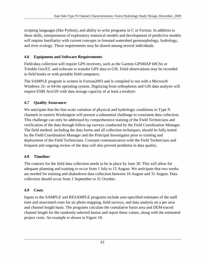
East Side Type N Channel Characterization: Forest Hydrology Study Design, December, 2009
61
scripting languages (like Python), and ability to write programs in C or Fortran. In addition to these skills, interpretation of exploratory statistical models and development of predictive models will require familiarity with current concepts in forested watershed geomorphology, hydrology, and river ecology. These requirements may be shared among several individuals.
4.6 Equipment and Software Requirements
Field-data collection will require GPS receivers, such as the Garmin GPSMAP 60CSx or Trimble GeoXT, and software to transfer GPS data to GIS. Field observations may be recorded in field books or with portable field computers.
The SAMPLE program is written in Fortran2003 and is compiled to run with a Microsoft Windows 32- or 64-bit operating system. Digitizing from orthophotos and GIS data analysis will require ESRI ArcGIS with data storage capacity of at least a terabyte.
4.7 Quality Assurance:
We anticipate that the fine-scale variation of physical and hydrologic conditions in Type N channels in eastern Washington will present a substantial challenge to consistent data collection. This challenge can only be addressed by comprehensive training of the Field Technicians and verification of the data through follow-up surveys conducted by the Field Coordination Manager. The field method, including the data forms and all collection techniques, should be fully tested by the Field Coordination Manager and the Principal Investigator prior to training and deployment of the Field Technicians. Constant communication with the Field Technicians and frequent and ongoing review of the data will also prevent problems in data quality.
4.8 Timeline:
The contract for the field data collection needs to be in place by June 30. This will allow for adequate planning and training to occur from 1 July to 15 August. We anticipate that two weeks are needed for training and shakedown data collection between 16 August and 31 August. Data collection should occur from 1 September to 31 October.
4.9 Costs
Inputs to the SAMPLE and RESAMPLE programs include user-specified estimates of the staff time and associated costs for air photo mapping, field surveys, and data analysis on a per area and channel length basis. The programs calculate the cumulative basin area and DEM-traced channel length for the randomly selected basins and report these values, along with the estimated project costs. An example is shown in Figure 18.
East Side Type N Channel Characterization: Forest Hydrology Study Design, December, 2009
62
Figure 18. Output from program SAMPLE for estimating study costs and time requirements. Estimated costs are based on values specified in the input file to SAMPLE and are shown here only to illustrate SAMPLE outputs, not as accurate cost estimates.
5 REFERENCES
Anderson, S.P., Dietrich, W.E., Montgomery, D.R., Torres, R., Conrad, M.E., and Loague, K., 1997, Subsurface flow paths in a steep, unchanneled catchment: Water Resources Research, v. 33, p. 2637-2653.
Beechie, T.J., Liermann, M., Pollock, M.M., Baker, S., and Davies, J., 2006, Channel pattern and river-floodplain dynamics in forested mountain river systems: Geomorphology, v. 78, p. 124-141.
Benda, L.E., Andras, K., Miller, D.J., and Bigelow, P., 2004a, Confluence effects in rivers: Interactions of basin scale, network geometry, and disturbance regimes: Water Resources Research, v. 40, p. W05402.
Benda, L.E., Miller, D.J., Bigelow, P., and Andras, K., 2003, Effects of post-wildfire erosion on channel environments, Boise River, Idaho: Forest Ecology and Management, v. 178, p. 105-119.
Benda, L.E., Miller, D.J., Dunne, T., Reeves, G.H., and Agee, J.K., 1998, Dynamic landscape systems, in Naiman, R.J., and Bilby, R.E., eds., River Ecology and Management: New York, Springer-Verlag, p. 261-288.
Benda, L.E., Poff, L., Miller, D.J., Dunne, T., Reeves, G.H., Pess, G.R., and Pollock, M.M., 2004b, The network dynamics hypothesis: how channel networks structure riverine habitats: BioScience, v. 54, p. 413-427.
Bent, G.C., and Steeves, P.A., 2006, A revised logistic regression equation and an automated procedure for mapping the probability of a stream flowing perennially in Massachusetts: U.S. Geological Survey Scientific Investigations Report 2006-5031, p. 107.
Input basin file headwater_all.dat Drainage Area threshold (km2) 0.1 Channel length threshold (m) 200 Proportion-of-area-in-FFR-lands threshold 0.25 Proportion-of-area-forested-threshold 0.75 Total number of basins in delineated population 117387 Number of basins meeting threshold criteria 15153 Number of samples 100 Cumulative basin area (sq mi) 26.04847 Cumulative traced channel length (miles) 129.644 Cumulative number of traced channel heads 340 Crew days for channel survey 45.63467 Estimated survey cost $ $95,725.36 Estimated analysis cost $ $27,604.58 Estimated total cost $ $131,829.90

East Side Type N Channel Characterization: Forest Hydrology Study Design, December, 2009
63
Breiman, L., Friedman, J.H., Olshen, R.A., and Stone, C.J., 1984, Classification and regression trees: Monterey, CA, Wadsworth & Brooks / Cole Advanced Books & Software.
Bren, L.J., 1997, Effects of slope vegetation removal on the diurnal variations of a small mountain stream: Water Resources Research, v. 33, p. 321-331.
Burnham, K.P., and Anderson, D.R., 2002, Model Selection and Multimodel Inference: New York, Springer, 488 p.
Butler, J.J.J., Kluitenbert, G.J., Whittemore, D.O., Loheide, S.P.I., Jin, W., Billinger, M.A., and Zhan, X., 2007, A field investigation of phreatophyte-induced fluctuations in the water table: Water Resources Research, v. 43.
Butturini, A., Bernal, S., Sabater, S., and Sabater, F., 2002, The influence of riparian-hyporheic zone on the hydrological responses in an intermittent stream: hydrology and earth System Sciences, v. 6, p. 515-525.
Castro, J.M., and Jackson, P.L., 2001, Bankfull discharge recurrence intervals and regional hydraulic geometry relationships: patterns in the Pacific Northwest, USA: Journal of the American Water Resources Association, v. 37, p. 1249-1262.
Clarke, S.E., Burnett, K.M., and Miller, D.J., 2008, Modeling streams and hydrogeomorphic attributes in Oregon from digital and field data: Journal of the American Water Resources Association, v. 44, p. 459-477.
Cochran, W.G., 1977, Sampling Techniques: New York, John Wiley & Sons, Inc, 428 p.
Colson, T.P., 2006, Stream network delineation from high-resolution digital elevation models [Dissertation thesis]: Raleigh, North Carolina, North Carolina State University.
Colson, T.P., Gregory, J.D., Mitasova, H., and Nelson, S.A.C., 2006, Comparison of stream extraction models using LiDAR DEMs, Geographic Information Systems and Water Resources IV, AWRA Spring Specialty Conference: Houston, Texas, AWRA, p. 7.
Conrad, R.H., Fransen, B., Duke, S., Liermann, M., and Needham, S., 2003, The development and assessment of the preliminary model for identifying fish habitat in western Washington: Olympia, WA, Cooperative Monitoring Evaluation & Research, p. 150.
Cupp, C.E., 2005, Water typing model field performance assessment pilot study: Olympia, Cooperative Monitoring Evaluation & Research, p. 21.
Daly, C., Halbleib, M., Smith, J.I., Gibson, W.P., Doggett, M.K., Taylor, G.H., Curtis, J., and Pasteris, P.P., 2008, Physiographically sensitive mapping of climatological temperature and precipitation acroos the conterminous United States: International Journal of Climatology.
De'ath, G., 2002, Multivariate regression trees: a new technique for modeling species-environment relationships: Ecology, v. 83, p. 1105-1117.
—, 2007, Boosted trees for ecological modeling and prediction: Ecology, v. 88, p. 243-251.
De'ath, G., and Fabricius, K.E., 2000, Classification and regression trees: a powerful yet simple technique for ecological data analysis: Ecology, v. 81, p. 3178-3192.
East Side Type N Channel Characterization: Forest Hydrology Study Design, December, 2009
64
Erskine, R.H., Green, T.R., Ramirez, J.A., and MacDonald, L.H., 2006, Comparison of grid-based algorithms for computing upslope contributing area: Water Resources Research, v. 42.
ESRI, 1998, ESRI Shapefile Technical Description, An ESRI White Paper, Environmental Systems Research Institute, Inc., p. 34.
Fransen, B.R., Duke, S.D., McWethy, L.G., Walter, J.K., and Bilby, R.E., 2006, A logistic regression model for predicting the upstream extent of fish occurrence based on geographical information systems data: North American Journal of Fisheries Management, v. 26, p. 960-975.
Friedman, J.H., 2002, Stochastic gradient boosting: Computional Statistics and Data Analysis, v. 38, p. 367-378.
Fritz, K., M., Johnson, B.R., and Walters, D.M., 2006, Field Operations Manual for Assessing the Hydrologic Permanence and Ecological Condition of Headwater Streams. EPA/600/R-06/126: Washington DC, US Environmental Protection Agency, Office of Research and Development.
—, 2008, Physical indicators of hydrologic permanence in forested headwater streams: Journal of the American Benthological Society, v. 27, p. 690-704.
Ganio, L.M., Torgersen, C.E., and Gresswell, R.E., 2005, A geostatistical approach for describing spatial pattern in stream networks: Frontiers in Ecology and the Environment, v. 3, p. 138-144.
Garbrecht, J., and Martz, L.W., 1997, The assignment of drainage direction over flat surfaces in raster digital elevation models: Journal of Hydrology, v. 193, p. 204-213.
Gomi, T., Sidle, R.C., and Richardson, J.S., 2002, Understanding processes and downstream linkages of headwater systems: BioScience, v. 52, p. 905-916.
Gooseff, M.N., Wondzell, S.M., and McGlynn, B.L., 2008, On the relationships among temporal patterns of evapo-transpiration, stream flow and riparian water levels in headwater catchments during baseflow, Integrating Groundwater Science and Human Well Being: Yoyama, Japan, p. 842-851.
Hall, J.E., Holzer, D.M., and Beechie, T.J., 2007, Predicting river floodplain and lateral channel migration for salmon habitat conservation: Journal of the American Water Resources Association, v. 43, p. 786-797.
Heine, R.A., Lant, C.L., and Sengupta, R.R., 2004, Development and comparison of approaches for automated mapping of stream channel networks: Annals of the Association of American Geographers, v. 94, p. 477-490.
Hodgson, M.E., and Bresnahan, P., 2004, Accuracy of airborne LiDAR-derived elevation: empirical assessment and error budget: Photogrammetric Engineering and Remote Sensing, v. 70, p. 331-339.

East Side Type N Channel Characterization: Forest Hydrology Study Design, December, 2009
65
Hodgson, M.E., Jensen, J., Raber, G., Tullis, J., Davis, B., Thompson, G., and Schuckman, K., 2005, An evaluation of Lidar-derived elevation and terrain slope in leaf-off conditions: Photogrammetric Engineering and Remote Sensing, v. 17, p. 817-823.
Hosmer, D.W., and Lemeshow, S., 2000, Applied Logistic Regression: New York, John Wiley & Sons, Inc., 375 p.
Hunter, M.A., Quinn, T., and Hayes, M.P., 2005, Low flow spatial characteristics in forested headwater channels of southwest Washington: Journal of the American Water Resources Association, v. 41, p. 503-516.
Jaeger, K.L., Montgomery, D.R., and Bolton, S.M., 2007, Channel and perennial flow initiation in headwater streams: management implications of variability in source-area size: Environmental Management, v. 40, p. 775-786.
Lancaster, S.T., and Casebeer, N.E., 2007, Sediment storage and evacuation in headwater valleys at the transition between debris-flow and fluvial processes: Geology, v. 35, p. 1027-1030.
MacCracken, J.G., and Boyd, W.C., undated report, Spatial and temporal variation in stream origins on Longview Fibre Company timberlands in Washington, Longview Fibre Company.
May, C.L., and Lee, D.C., 2004, The relationships among in-channel sediment storage, pool depth, and summer survival of juvenile salmonids in Oregon Coast Range streams: North American Journal of Fisheries Management, v. 24, p. 761-774.
McCleary, R.J., and Hassan, M.A., 2008, Predictive modeling and spatial mapping of fish distributions in small streams of the Canadian Rocky Mountain foothills: Canadian Journal of Fisheries and Aquatic Science, v. 65, p. 319-333.
McGuire, K.J., McDonnell, J.J., Weiler, M., Kendall, C., McGlynn, B.L., Welker, J.M., and Seibert, J., 2005, The role of topography on catchment-scale water residence time: Water Resources Research, v. 41.
McNamara, J.P., Ziegler, A.D., Wood, S.H., and Vogler, J.B., 2006, Channel head locations with respect to geomorphologic thresholds derived from a digital elevation model: a case study in northern Thailand: Forest Ecology and Management, v. 224, p. 147-156.
Miller, D.J., and Burnett, K.M., 2008, A probabilistic model of debris-flow delivery to stream channels, demonstrated for the Coast Range of Oregon, USA: Geomorphology, v. 94, p. 184-205.
Miller, J.F., Frederick, R.H., and Tracey, R.J., 1973, NOAA ATLAS 2: Precipitation-Frequency Atlas of the Western United States, Volume 9, Washington, National Oceanic and Atmospheric Administration, 43 p.
Montgomery, D.R., and Dietrich, W.E., 1989, Source areas, drainage density, and channel initiation: Water Resources Research, v. 25, p. 1907-1918.
—, 2002, Runoff generation in a steep, soil-mantled landscape: Water Resources Research, v. 38, p. 1168.

East Side Type N Channel Characterization: Forest Hydrology Study Design, December, 2009
66
Montgomery, D.R., and Foufoula-Georgiou, E., 1993, Channel network source representation using digital elevation models: Water Resources Research, v. 29, p. 3925-3934.
Moore, R.D., and Wondzell, S.M., 2005, Physical hydrology and the effects of forest harvesting in the Pacific Northwest: a review: Journal of the American Water Resources Association, v. 41, p. 763-784.
Mouton, A., 2005, Generating Stream Maps Using LiDAR Derived Digital Elevation Models and 10-m USGS DEM: Seattle, WA, University of Washington.
Murphy, P.N.C., Ogilvie, J., Meng, F.-R., and Arp, P., 2008, Stream network modelling using lidar and photogrammetric digital elevation models: a comparison and field verification: Hydrological Processes, v. 22, p. 1747-1754.
Neeson, T.M., Gorman, A.M., Whiting, P.J., and Koonce, J.F., 2008, Factors affecting accuracy of stream channel slope estimates derived from geographical information systems: North American Journal of Fisheries Management, v. 28, p. 722-732.
North Carolina Division of Water Quality, 2008, Mapping headwater streams: intermittent and perennial headwater stream model development and spatial application, North Carolina division of Water Quality, p. 54.
O'Callaghan, J.F., and Mark, D.M., 1984, The extraction of drainage networks from digital elevation data: Computer Vision, Graphics, and Image Processing, v. 28.
OHEPA, O.E.P.A., 2002, Field evaluation manual for Ohio's primary headwater habitat streams. Final Version Columbus, Ohio, Division of Surface Water, Ohio Environmental Protection Agency.
Palmquist, R., 2005, Type N Stream Demarcation Study, Phase 1: Pilot Results, CMER, p. 61.
Pike, R.G., and Scherer, R., 2003, Overview of the potential effects of forest management on low flows in snowmelt-dominated hydrologic regimes: BC Journal of Ecosystems and Management, v. 3, p. 44-60.
Pleus, A.E., and Goodman, P., 2003, Type N stream demarcation study: 2002 tribal perennial stream survey data collection using CMER methods, Northwest Indian Fisheries Commission, p. 53.
Ralph, S.C., Poole, G.C., Loveday, L.C., and Naiman, R.J., 1994, Stream channel morphology and woody debris in logged and unlogged basins of western Washington: Canadian Journal of Fisheries and Aquatic Science, v. 51, p. 37-51.
Robinson, T.W., 1958, Phreatophytes, in Survey, G., ed., Volume Water-Supply Paper 1423, U.S. Geological Survey.
SAGE, 2007, Scoping Document, Eastside Forest Hydrology: A proposed study for the Eastside Type N Characterization Project, CMER.
Stock, J.D., and Dietrich, W.E., 2003, Valley incision by debris flows: Evidence of a topographic signature: Water Resources Research, v. 39, p. doi:10.1029/2001WR001057.

East Side Type N Channel Characterization: Forest Hydrology Study Design, December, 2009
67
Terrapin Environmental, 2004, Water typing model field performance assessment approach and procedures: Olympia, WA, Cooperative Monitoring Evaluation & Research, p. 30.
Topping, B.J.D., Nadeau, T.-L., and Turaski, M.R., 2009, Oregon streamflow duration assessment method interim version.
Veldhuisen, C., 2000, Preliminary results and recommendations from the northwest Cascades Type 4/5 stream study, Skagit System Cooperative, p. 6.
—, 2004, Summary of headwater perennial stream surveys in the Skagit and neighboring basins: 2001-2003, Skagit River System Cooperative, p. 10.
Wing, M.G., and Skaugset, A.E., 2002, Relationships of channel characteristics, land ownership, and land use patterns to large woody debris in western Oregon streams: Canadian Journal of Fisheries and Aquatic Science, v. 59, p. 796-807.
Winter, T.C., 2007, The role of ground water in generating streamflow in headwater areas and in maintaining base flow: Journal of the American Water Resources Association, v. 43, p. 15-25.
Zevenbergen, L.W., and Thorne, C.R., 1987, Quantitative analysis of land surface topography: Earth Surface Processes and Landforms, v. 12, p. 47-56.