LANDSLIDE TSUNAMI HAZARD ALONG THE UPPER

U.S. EAST COAST: EFFECTS OF SLIDE

RHEOLOGY AND BOTTOM FRICTION

BY

LAUREN SCHAMBACH1, STEPHAN T. GRILLI1,

JAMES T. KIRBY2, AND FENGYAN SHI2

1 DEPARTMENT OF OCEAN ENGINEERING, UNIVERSITY OF RHODE ISLAND

2 CENTER FOR APPLIED COASTAL RESEARCH, DEPARTMENT OF CIVIL AND

ENVIRONMENTAL ENGINEERING, UNIVERSITY OF DELAWARE

RESEARCH REPORT NO. CACR-17-04

OCTOBER 2017

RESEARCH SUPPORTED BY THE NATIONAL TSUNAMI HAZARD MITIGATION PROGRAM

(NOAA) UNDER GRANTS NA-15-NWS4670029 AND NA-16-NWS4670034

CENTER FOR APPLIED COASTAL RESEARCH

University of Delaware

Newark, Delaware 19716

Abstract

We perform numerical simulations to assess tsunami hazard along the upperUS East Coast (USEC; From Virginia to Cape Cod, MA), caused by Subma-rine Mass Failures (SMFs) triggered on the continental shelf slope, consideringthe effect of SMF rheology, i.e., whether the SMFs behave as rigid slumps ordeforming slides. We simulate tsunami generation using the three-dimensionalnon-hydrostatic model NHWAVE. For rigid slumps, the geometry and law of mo-tion are specified as bottom boundary conditions and for deforming slides SMFmotion and deformation are modeled in a depth-integrated bottom layer of denseNewtonian fluid, fully coupled to the overlying fluid motion. Once the SMFs areno-longer tsunamigenic, we continue simulating tsunami propagation using thetwo-dimensional fully nonlinear and dispersive long wave model FUNWAVE-TVD. For the onshore tsunami propagation, we use nested grids of increasinglyfine resolution towards shore and apply a one-way coupling methodology. As inearlier work, we only simulate probable maximum tsunamis generated by Cur-rituck SMF proxies, i.e., SMFs having the same volume and footprint as the his-torical Currituck slide complex, the largest known on the USEC. These proxiesare sited in four areas of the shelf break slope identified to have enough sedi-ment accumulation to cause large failures. In tsunami generation simulations,we find that deforming slides have a slightly larger initial acceleration, but stillgenerate a smaller tsunami than rigid slumps due to their spreading and thinningout during motion, which gradually makes them less tsunamigenic; by contrast,rigid slumps keep their specified shape during their pendulum-like motion. Wecompare the combined maximum envelope of surface elevation caused along theshore (5 m isobath) by these SMF tsunamis. Consistent with earlier work, wefind that the bathymetry of the wide shelf strongly controls the magnitude oftsunami coastal inundation, as it induces wave focusing and defocusing effects.Additionally, tsunami propagation and refraction over the shelf, both north andsouth of each source area, causes non-trivial variations in surface elevation andcoastal inundation. As a result, SMF tsunamis can cause a significant coastalimpact far alongshore from their source area. Overall, tsunamis caused by rigidslumps are worst case scenarios (absolute maximum inundation about 11.5 maround Montauk, NY), providing up to 50% more inundation than for slideshaving a moderate level of deformation (viscosity set in the upper range of de-bris flows). Regarding minimum elevations at the coast, which affect power plantintakes, tsunamis from both types of SMFs are shown to be able to cause waterwithdrawal to the 5 m isobath or deeper. Finally, bottom friction effects are as-sessed by performing some simulations using two different Manning coefficients,one 50% larger than the other; with the increased friction, the largest tsunamiinundations at the coast are reduced, in some cases, by up to 15%.

Contents

1 Introduction 1

2 Modeling methodology 5

2.1 Numerical models . . . . . . . . . . . . . . . . . . . . . . . . . . . . . . 5

2.2 Computational grids . . . . . . . . . . . . . . . . . . . . . . . . . . . . 6

3 SMF tsunami generation with NHWAVE(D) 8

3.1 SMF geometry, rheology and kinematics . . . . . . . . . . . . . . . . . 8

3.2 Tsunami generation . . . . . . . . . . . . . . . . . . . . . . . . . . . . . 14

4 Onshore tsunami propagation and coastal impact 17

4.1 Instantaneous propagation and time series . . . . . . . . . . . . . . . . 17

4.2 Maximum and minimum surface elevations . . . . . . . . . . . . . . . . 24

5 Discussion and conclusions 25

A SMF geometry and slump law of motion 32

List of Figures

1 Geography of study area (with marked state limits and names, andnames of a few cities (red stars) identified). Areas 1-4, identified by(Grilli et al., 2015) as having high potential for large tsunamigenic SMFs,and the location of the historical Currituck slide complex are marked byyellow ellipses. Numerical gage stations 1-7 (20 m depth) are marked byyellow bullets. The color scale and bathymetric contours show depth inmeters. . . . . . . . . . . . . . . . . . . . . . . . . . . . . . . . . . . . . 2

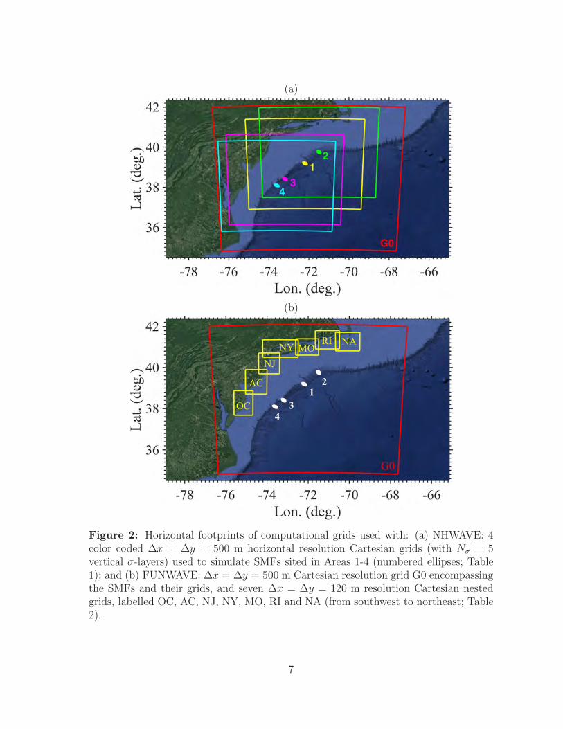
2 Horizontal footprints of computational grids used with: (a) NHWAVE:4 color coded ∆x = ∆y = 500 m horizontal resolution Cartesian grids(with Nσ = 5 vertical σ-layers) used to simulate SMFs sited in Areas1-4 (numbered ellipses; Table 1); and (b) FUNWAVE: ∆x = ∆y = 500m Cartesian resolution grid G0 encompassing the SMFs and their grids,and seven ∆x = ∆y = 120 m resolution Cartesian nested grids, labelledOC, AC, NJ, NY, MO, RI and NA (from southwest to northeast; Table2). . . . . . . . . . . . . . . . . . . . . . . . . . . . . . . . . . . . . . . 7

3 Vertical bathymetric transects in each NHWAVE grid (Fig. 2a), throughAreas 1-4 (plots a-d) SMF centers (x0, y0), in azimuthal direction θ (Ta-ble 1): (solid black) current bathymetry; (dash blue) initial SMF profile;(solid red) final slump profile after displacement (runout) Sf = 15.8 kmat tf = 715 s (11.9 min); (solid green/dash green) deforming slide pro-files at t = 715 and 1,200 s (20 min). The x-axis measures distancesfrom each SMF center; vertical exaggeration is 25 times. . . . . . . . . 9

4 Kinematics of Currituck SMF proxies sited in Areas 1-4 (Fig. 1), duringtsunami generation. SMF center of mass: (a) motion; (b) velocity;and (c) acceleration, specified for rigid slumps (black) modeled withNHWAVE (based on Eqs. (4) to (10) in Appendix A), and computedfor deforming slides modeled with NHWAVED (for νs = 0.5 m2/s andn = 0.1), in Area: (ochre) 1; (green) 2; (purple) 3; (turquoise) 4. . . . . 12

5 Instantaneous 3D geometry (grey volume) of Currituck SMF proxy inArea 1 (Fig. 1), simulated with NHWAVE(D) in a 500 m resolutiongrids with Nσ = 5 vertical layers (Fig. 2a), modeled as a: (a, c, e)deforming slide; or (b, d, f) rigid slump, at t = (a, b) 5, (c, d) 10, and(e, f) 15 min. The vertical axis denotes depth in meter. . . . . . . . . . 13

6 Snapshots of free surface elevations (color scale in m) simulated at t =800 s (13.3 min) with NHWAVE(D), in 500 m grids (Fig. 2a; Table 1),for four Currituck SMF proxies modeled as: (a, c, e, g) rigid slumps(similar to Grilli et al., 2015); or (b, d, f, h) deforming slides (with νs =0.5 m/s2, n = 0.1), sited in Areas 1-4 (Fig. 1). Black ellipses mark initialfootprints of each SMF (Table 1), which all have a volume Vs = 158 km3,density ρs = 1900 kg/m3, and similar runout Sf at tf = 715 s (when theslumps stop moving). . . . . . . . . . . . . . . . . . . . . . . . . . . . . 15

7 Spatial variation of friction coefficient Cd = g n2/h1/3 (color scale) usedin FTVD simulations, based on local depth h (contour lines in meter)and Manning coefficient n = (a) 0.025 over grid G0 (Fig. 2); (b, c) 0.025and 0.0375 s2/m2/3), respectively, over grid NJ (Fig. 2b; Table 2). Note,a minimum depth of 0.1 m is assumed in the Cd calculations. . . . . . . 16

8 Instantaneous free surface elevations (color scale in m) simulated withNHWAVE and FTVD in grid G0 (Fig. 2) for the deforming CurrituckSMF proxy in Area 1 (Figs. 1 and 6b) at t = 10, 30, 50, 70, 90, 110, 130,and 150 min (from left to right, up to down). Circles mark locations ofgage stations 1-7 (Fig. 1). Black contours mark depth in meter. . . . . 18

9 Time series of free surface elevation simulated with NHWAVE and FTVDin grid G0 (Fig. 2) at: (a-g) wave gage stations 1-7, as: (solid lines) rigidslumps; or (dash lines) deforming, Currituck SMF proxies, sited in Areas(Fig. 1): (ochre) 1; (green) 2; (purple) 3; and (turquoise) 4. All sta-tions are located in 20 m depth and are at (Lon., Lat.): (1) (-75.30289,37.67788); (2) (-74.68185, 38.83211); (3) (-73.99977, 39.74429); (4) (-73.39142, 40.52213); (5) (-72.48927, 40.80720); (6) (-71.49228, 41.31645);(7) (-70.67353, 41.31252). . . . . . . . . . . . . . . . . . . . . . . . . . . 19

10 (a,b) Envelopes of maximum surface elevations (color scale in m) com-puted with FTVD in 120 m grid NJ (Fig. 2; Table 2), for the deformingCurrituck SMF proxy sited in Area 1 (Figs. 1, 6b, and 8), with a Man-ning n = (a) 0.025; or (b) 0.0375 s2/m2/3 (Figs. 7b,c). Black contoursmark depth in meter. (c,d) zoom-in on the coastline and barrier beachesaround Seaside Heights, NJ (c) and Long Beach, NY (d), both markedby red stars. White contours mark depth in meter . . . . . . . . . . . . 21

11 Combined envelope of maximum surface elevations (color scale in m)computed with FTVD in 500 m grid G0 or 120 m nested grids whereveravailable (Fig. 2b; Table 2), for the four SMFs sited in areas 1-4 (Fig.1): (a) deforming slides; or (b) rigid slumps. The white lines markthe 5 m isobath along which maximum and minimum wave heights arecomputed (see, Fig. 12). Black contours mark depth in meter. . . . . . 22

12 (a,b) Maximum and (c) minimum surface elevation computed along the5 m isobath (Fig. 11) for tsunamis generated by: (blue) rigid slump inArea 1 (a), or combined slumps in Areas 1-4 (b,c); and (red) deformingslide in Area 1 (a), or combined deforming slides in Areas 1-4 (b,c). AllFUNWAVE simulations are performed with n = 0.025 s2/m2/3; greenline in plot (a) is deforming slide in Area 1 for n = 0.0375 s2/m2/3

(Fig. 7). The distance s is the curvilinear distance along the 5 misobath measured from its southern end. Labels mark entrance to: (DB)Delaware Bay; (NYH) New York Harbor; (LIS) Long Island Sound; (NB)Narragansett Bay; (BB) Buzzards Bay. . . . . . . . . . . . . . . . . . . 23

13 Geometric parameterization of a SMF initially centered at (x0, y0) mov-ing in direction ξ, with an azimuth angle θ from North and center ofmass motion S(t) measured parallel to the mean local slope of angleα; (x, y) denote the longitudinal and latitudinal horizontal directions,respectively. . . . . . . . . . . . . . . . . . . . . . . . . . . . . . . . . . 34

List of Tables

1 Parameters of NHWAVE grids (∆x = ∆y = 500 m resolution; Nσ = 5σ-layers; 1,000 by 1,000 cells), and locations (center) of SMFs of widthb = 30 km, width w = 20 km and thickness T = 0.75 km, in Areas 1-4(Figs. 1 and 2a). For rigid slumps, the average local slope is assumedto be α = 4 deg. (Fig. 3). . . . . . . . . . . . . . . . . . . . . . . . . . 8

2 Parameters of FUNWAVE-TVD computational grids (Fig. 2) . . . . . . 8

1 Introduction

This study was performed as part of tsunami hazard assessment work carried outsince 2010 under the auspices of the US National Tsunami Hazard Mitigation Pro-gram (NTHMP). In this work, the authors developed tsunami inundation maps forthe US East Coast (USEC), by modeling tsunami generation, propagation, and coastalimpact for a series of extreme sources selected in the Atlantic Ocean basin (Grilliet al., 2010; Tehranirad et al., 2015; Grilli et al., 2017a), to trigger so-called Prob-able Maximum Tsunamis (PMTs). These inundation maps thus represent the en-velope of maximum inundation resulting from the combined coastal impact of thesetsunamis, without consideration of return periods (ECMAP, 2017; Tehranirad et al.,2014, 2015a,b,c,d,e). Tsunami generation and propagation were simulated using two-dimensional (2D) Boussinesq (Shi et al., 2012; Kirby et al., 2013) and three-dimensional(3D) non-hydrostatic (Ma et al., 2012) wave models, in a series of nested spherical andCartesian grids of increasingly fine resolution towards the coast. These grids were builtusing commensurately accurate bathymetric and topographic data, the finer coastalgrids typically having a 10-30 m resolution.

This work, as well as other earlier studies, showed that along the upper USEC thehazard is dominated by near-field tsunamis that could potentially be generated by largesubmarine mass failures (SMFs) (ten Brink et al., 2008, 2009a,b; Grilli et al., 2009; tenBrink et al., 2014; Grilli et al., 2015, 2017a,b). The moderate seismicity typical of theregion would not be expected to cause significant near-field co-seismic tsunamis, butcould trigger large SMFs, particularly where sediment accumulates over steep slopes onthe continental shelf break, off of major estuaries. In fact, the largest earthquake evermeasured in the USEC area, with a Mw 7.2 magnitude, was responsible for triggeringthe 1929 landslide tsunami off of the Grand Banks (Piper et al., 1999; Fine et al., 2005).With a maximum runup of 13 m, this tsunami caused widespread destruction of coastalcommunities and 28 casualties in Newfoundland. The SMF displaced over 100 km3 ofsediment, turning into a turbidity current that reached speeds of 17-28 m/s, breaking12 underwater communication cables in the process. Confirming that the 1929 landslidewas not an isolated event, ten Brink et al. (2014) mapped numerous paleo-SMFs onthe US Atlantic continental shelf and margin, with the largest one being the Currituckslide complex (Locat et al., 2009), off of Chesapeake Bay (Fig. 1). If it had failedin present days, this paleo-SMF would have generated a destructive tsunami for theupper USEC (Geist et al., 2009; Grilli et al., 2015). Recent field work (Hill et al., 2017)has dated this old slide complex to 16-50Ka, but Chaytor (personal communication)indicates that its age is likely on the younger end of this range. Considering when thisfailure occurred, the sea level would have been much lower than in present days.

To assess SMF tsunami hazard along the USEC, Grilli et al. (2009) performedMonte Carlo Simulations (MCS) of SMFs triggered by seismicity along a series of tran-sects defined perpendicular to the coastline. These were initially sited from southernNew Jersey to Cape Cod, MA, but the study was later extended by Krauss (2011) tosouthern Florida, yielding a total of 91 transects for the entire USEC. In the MCS, thou-

1

Figure 1: Geography of study area (with marked state limits and names, and namesof a few cities (red stars) identified). Areas 1-4, identified by (Grilli et al., 2015) ashaving high potential for large tsunamigenic SMFs, and the location of the historicalCurrituck slide complex are marked by yellow ellipses. Numerical gage stations 1-7(20 m depth) are marked by yellow bullets. The color scale and bathymetric contoursshow depth in meters.

2

sands of potential SMFs were generated along each transect, with associated randomvalues of geometry, sediment properties, mechanism–slide or slump–, depth, and excesspore pressure, selected from assumed probability distributions and/or site specific fielddata. The selection of a failure mechanism was entirely based on the sediment nature,with slumps being associated with cohesive clay-type sediments and slides with non- (orless-)cohesive silt-type sediments. Local seismicity was randomly selected from USGSdata (i.e., from curve fitted probability distributions of peak horizontal acceleration).Standard slope stability analyses were performed for each potential failure and, forunstable cases, tsunami generation and runup were calculated based on semi-empiricalequations developed by Watts et al. (2005). At the time, it was not thought possibleto apply actual tsunami generation and propagation models to such a large numberof cases. These results allowed estimating the 100 and 500 year return period SMFtsunami runups along the entire USEC, which predicted a 500 year runup of up to 5-6m north of Virginia and a significantly reduced runup south of it. Eggeling (2012) usedthese results as guidance to carry out geophysical and geotechnical analyses on seafloordata collected in regions facing segments of the coast with the largest runup. This ledto selecting four areas (Fig. 1) where, given sufficient seismicity, large tsunamigenicSMFs could be expected to occur. These areas typically had a large bottom slope anda sediment thickness sufficient to make a large failure possible. More detailed slope sta-bility analyses, performed using the model SLIDE (SLIDE, 2017), yielded low factorsof safety in these areas, confirming the high likelihood of failure.

As part of their NTHMP inundation mapping work, which was based on PMTs,Grilli et al. (2015) modeled SMF tsunami hazard along the upper USEC by simu-lating tsunami generation from large SMFs sited in Areas 1-4 identified by Eggeling(2012) (Fig. 1), using the 3D non-hydrostatic model NHWAVE (Ma et al., 2012). Inthe absence of detailed site specific information, these were parameterized using thecharacteristics of the largest known historical failure in the region, i.e., the Currituckslide complex (Fig. 1); for this reason they are referred to as “Currituck SMF proxy”sources. The Currituck slide complex has been extensively studied from geologicaland slide triggering points of views (e.g., Locat et al. (2009), and references herein).Tsunami generation from a reconstituted Currituck SMF was first modeled by Geistet al. (2009), using a simplified SMF tsunami generation model. To maximize tsunamigeneration, Grilli et al. (2015) considered that each Currituck SMF proxy was madeof a single large failure, with a volume in the 128-165 km3 range estimated for thewhole Currituck slide complex by Locat et al. (2009). They assumed that each SMFfailed as a rigid slump, which based on earlier work was expected to maximize tsunamigeneration and coastal impact (Grilli and Watts, 2005). In the slump law of motion,they used the maximum velocity of the SMF center of mass estimated by Locat et al.(2009) (≃ 35 m/s). Once the slumps had stopped moving and tsunami generation wascomplete, simulations of tsunami propagation and coastal impact were performed usingthe 2D Boussinesq model FUNWAVE-TVD (Shi et al., 2012) (referred to hereafter asFTVD), in a series of nested grids. Results of these simulations were used to developthe NTHMP tsunami inundation maps currently released for the upper USEC region

3

(ECMAP, 2017).

More recently, Grilli et al. (2017b) investigated the effects of SMF kinematics andrheology on tsunami hazard, using the newer two-layer version of NHWAVE (Kirby etal., 2016), referred to here as NHWAVED (for NHWAVE deforming). In this model,deforming slides are modeled as a dense Newtonian fluid, in a depth-integrated bottomlayer, and the coupled upper water layer flow is simulated with the standard multi-σ-layers NHWAVE model. Grilli et al. (2017b) first simulated the historical CurrituckSMF with this model, to estimate relevant values of slide viscosity νs and bottomfriction Manning coefficient, n (between slide and substrate). This was done by findingvalues that yielded a slide center of mass motion S(t) similar to that Grilli et al. (2015)used in rigid slump simulations, and a maximum runout Sf similar to the slump, aftera time of motion tf . They inferred a fairly large viscosity (νs = 0.5 m2/s), whichwas then used to model the Currituck SMF proxy in Area 1 (Hudson River canyon)as a deforming slide. Comparing the computed maximum surface elevation nearshore(over the 5 m isobath) to that caused by the rigid slump, they found that, despite thehigh viscosity, due to the spreading-out of the deforming slide during its motion, theSMF acceleration and related maximum tsunami elevations were reduced as comparedto the rigid slump. Also because the deforming slide flowed on its own (rather thanhaving its motion prescribed), it followed the steepest bottom slope and the generatedtsunami ended up being more asymmetrical than for the slump. This latter featureaffects where maximum tsunami impact occurs along the coast, and hence the levelof hazard. They concluded that modeling tsunami hazard by considering that all theSMF fail as rigid slumps was likely too conservative, although the opposite could betrue in some site specific situations. Hence, it should be more realistic (i.e., in betteragreement with field observations in the region) to consider tsunami generation fromdeforming slides, even if only a moderate level of deformation (i.e., a high viscosity) isconsidered.

In light of these conclusions, in this paper, we follow a methodology similar tothat of Grilli et al. (2017b) to more realistically assess landslide tsunami hazard alongthe upper USEC (from Virginia to Massachusetts), by modeling tsunami generationand propagation from Currituck SMF proxies sited in Areas 1-4 (Fig, 1), failing asdeforming slides. For comparison, since we use higher-resolution computational grids,we also recompute tsunami generation and propagation for the same SMFs failing asrigid slumps (as in Grilli et al. (2015)). Additionally, since earlier work indicated asignificant effect of bottom friction on tsunami propagation for wide shelves (Geist etal., 2009; Grilli et al., 2015; Tehranirad et al., 2015), unlike Grilli et al. (2015) who useda constant bottom friction coefficient value Cd = 0.0025 in their FTVD simulations, weuse a depth-dependent value of Cd, modeled with Manning’s formula, as a function ofManning’s coefficient n. We use n = 0.025 s2/m2/3 throughout, but also compare theresulting tsunami coastal impact for n = 0.025 and 0.0375, in one of the most impactedareas of the USEC, in northern New Jersey and western Long Island, NY. Results areprovided as instantaneous surface elevations maps, time series of surface elevation atnumerical wave gages, and envelopes of tsunami surface elevations, for the combination

4

of the 4 SMFs. This allows assessing tsunami hazard from extreme SMFs, along theUSEC from Virginia to Cape Cod, MA.

In the following, in Section 2, we summarize the modeling methodology, in Section3, we present simulations of SMF tsunami generation with NHWAVE and in Section4, of SMF tsunami propagation and coastal impact with FTVD; this is followed by adiscussion with conclusions in Section 5.

2 Modeling methodology

2.1 Numerical models

Tsunami generation by SMFs is modeled using the 3D non-hydrostatic model NHWAVE(Ma et al., 2012), when considering rigid SMFs of specified center of mass motion, andthe newer two-layer NHWAVED model (Kirby et al., 2016), when simulating deformingSMFs as a dense Newtonian fluid. In both cases, the model uses a horizontal Cartesiangrid of resolution (∆x,∆y) and a boundary fitted σ-coordinate grid, with Nσ layersin the vertical direction. Once the tsunami is fully generated (this will be discussedbelow), the modeling of wave propagation is pursued with the 2D fully nonlinear anddispersive long wave Boussinesq model FTVD; because only regional grids of small geo-graphic extent are considered, the Cartesian coordinate version of FTVD was used(Shiet al., 2012). As in earlier work, FTVD simulations are performed by one-way couplingin a series of nested grids of increasingly fine resolution (see, e.g., Grilli et al. (2013,2015, 2017a,b); Tappin et al. (2014); Shelby et al. (2016), for details and examples ofthis approach).

Both NHWAVE(D) and FTVD are non-hydrostatic, i.e., dispersive, wave models.Numerous earlier works have clearly identified the importance of including frequencydispersion effects in the modeling of SMF tsunami generation and propagation, essen-tially due to the typically smaller wavelength to depth ratio of the generated waves(see, e.g.,Grilli and Watts (1999, 2005); Tappin et al. (2008); Ma et al. (2012)) In par-ticular, Tappin et al. (2008) and Ma et al. (2012) showed that turning off dispersionin their landslide tsunami simulations caused large errors on the shape and kinematicsof the generated waves. Additionally, without dispersion in the models the generatedwave trains lacked in constructive-destructive wave-wave interactions during propaga-tion, leading to significant errors in wave height and steepness when reaching shallowwater; the generated wave trains also typically lacked the oscillatory (dispersive) boresand tails observed for landslide tsunamis, experimentally (see references listed in Grilliet al. (2017b)), in the field (e.g., Tappin et al. (2014)), or numerically (e.g., Tappin etal. (2008); Løvholt et al. (2008); Abadie et al. (2012); Grilli et al. (2015); Tehraniradet al. (2015)), and were limited to one or two leading waves.

To specify the geometry and kinematics of rigid slumps, we follow the method-ology detailed in Grilli et al. (2015), in which these are specified as bottom boundaryconditions in NHWAVE (see also Grilli and Watts (2005); Watts et al. (2005); Enet and

5

Grilli (2007)). In addition to the references, a summary of this methodology is givenin Appendix A. For deforming slides, as in Grilli et al. (2017b), we use NHWAVEDwhere the SMFs are modeled as a layer of dense fluid, couple, along the SMF-waterinterface with an upper water layer represented by σ-layers and a free surface, as inNHWAVE. In the bottom layer, SMF equations of mass and momentum conservationare depth-integrated, similar to those obtained in a long wave generation model, andinclude both volumetric (i.e., viscous) and bottom friction dissipation terms. The ge-ometry of both rigid and deforming SMFs is modeled as an initial sediment moundof quasi-Gaussian cross-sections and elliptical footprint over the slope (see, Enet andGrilli (2007); Grilli et al. (2015), and Appendix A Eqs. (1) to (3), for details).

For rigid slumps, tsunami generation ends when the SMF reaches its maximumrunout and stops moving. Deforming slides, however, keep moving (i.e., flowing) for amuch longer time down the continental slope. Hence, at the time selected to continuesimulations with FTVD (here 20 min), deforming slides are still moving and hence atime dependent bottom boundary condition is specified on NHWAVED’s bottom. Grilliet al. (2017b) observed, in their coarser grid simulations of deforming slides in Area1, that when initializing FTVD using results computed in NHWAVED with this non-homegeneous bottom boundary condition, spurious (rebound) waves were generatedoffshore in FTVD. They circumvented this problem by filtering out velocities over thelocation of the slide, before initializing FTVD. Because the slide was far offshore atthis time and no-longer tsunamigenic, this did not affect simulations of the tsunamionshore propagation. A similar method is used in the present simulations.

2.2 Computational grids

SMF tsunami generation is computed with NHWAVE(D) in Areas 1-4, in four distinctCartesian grids centered around each SMF (Fig. 2a). Each grid has a ∆x = ∆y = 500m horizontal resolution, Nσ = 5 σ-layers in the vertical direction, and covers a 500 by500 km footprint (i.e., each has 1,000 by 1,000 cells; see SW corner coordinates in Table1). NHWAVE(D)’s Cartesian grid coordinates and bathymetry are constructed bymapping, with the projection center in each grid specified at each SMF initial location(x0, y0) (Table 1). NHWAVE(D)’s grids are all embedded within the ∆x = ∆y = 500m Cartesian grid G0 that is the first-level (or base) grid used in FTVD to continuesimulations of tsunami propagation; this grid covers an 800 km by 800 km area and,hence, has 1,600 by 1,600 cells (Fig. 2; see details in Table 2). After tsunami waveshave been generated with NHWAVE(D), the surface elevation, bottom bathymetry,and (u, v) horizontal velocities (at the required depth of 0.531h for FTVD; Shi et al.(2012)), computed for each case, are interpolated onto FTVD’s grid G0. These initialconditions are used to continue simulations of tsunami wave propagation to shore foreach SMF, in grid G0 and then in 7 nested Cartesian grids of resolution ∆x = ∆y = 120m (Fig. 2b; Table 2). To eliminate reflection at its offshore boundary, 125 km thicksponge layers are specified on both the eastern and southern boundaries of grid G0.

The bathymetry used in each grid is interpolated from the 3-arc second (≃ 90

6

(a)

(b)

Figure 2: Horizontal footprints of computational grids used with: (a) NHWAVE: 4color coded ∆x = ∆y = 500 m horizontal resolution Cartesian grids (with Nσ = 5vertical σ-layers) used to simulate SMFs sited in Areas 1-4 (numbered ellipses; Table1); and (b) FUNWAVE: ∆x = ∆y = 500 m Cartesian resolution grid G0 encompassingthe SMFs and their grids, and seven ∆x = ∆y = 120 m resolution Cartesian nestedgrids, labelled OC, AC, NJ, NY, MO, RI and NA (from southwest to northeast; Table2).

7

Grids and SMFs Area 1 Area 2 Area 3 Area 4

SW corner (Lon., Lat.) (-75.00, 36.90) (-74.32, 37.47) (-75.97, 36.12) (-76.37, 35.80)center (x0, y0) (-72.19, 39.19) (-71.49, 39.76) (-73.19, 38.41) (-73.6, 38.09)

Azimuth θ (CW from N) 136◦ 153◦ 140◦ 126◦

Table 1: Parameters of NHWAVE grids (∆x = ∆y = 500 m resolution; Nσ = 5σ-layers; 1,000 by 1,000 cells), and locations (center) of SMFs of width b = 30 km,width w = 20 km and thickness T = 0.75 km, in Areas 1-4 (Figs. 1 and 2a). For rigidslumps, the average local slope is assumed to be α = 4 deg. (Fig. 3).

Grid Name Cells (Mx,Ny) Resol. (m) SW Corner (Lat., Lon.)

Base Grid (G0) (1600, 1600) 500 (34.82N, 76.37W)Ocean City (OC) (672, 1104) 120 (37.68N, 75.60W)Atlantic City (AC) (752, 1104) 120 (38.70N, 75.04W)New Jersey (NJ) (720, 936) 120 (39.70N, 74.40W)New York (NY) (1212, 792) 120 (40.49N, 74.21W)Montauk (MO) (780, 744) 120 (40.60N, 72.60W)

Rhode Island (RI) (816, 828) 120 (40.90N, 71.65W)Nantucket (NA) (828, 832) 120 (40.81N, 70.67W)

Table 2: Parameters of FUNWAVE-TVD computational grids (Fig. 2)

m) resolution Northeast Atlantic and Southeast Atlantic U.S. Coastal Relief Models(NGDC, 1999a,b), wherever available (mostly up to the shelf break), and otherwisefrom the 1-arc minute resolution ETOPO-1 Global Relief Model (Amante and Eakins,2009). The latter bathymetric data is plotted in Fig. 1, as both a color scale andcontour lines, showing the typical pattern of the wide shallow USEC shelf (depthh ≤ 100m) north of North Carolina, a steep shelf break slope and a deep abyssal plain(h = 2, 000 to 5,000 m). Similar to the Currituck slide complex, the four study areas1-4 are all located on the shelf break slope.

3 SMF tsunami generation with NHWAVE(D)

3.1 SMF geometry, rheology and kinematics

As discussed above, we model tsunami generation by Currituck SMF proxies sited inAreas 1-4 off of the USEC (Fig. 1), assumed to fail as rigid slumps (similar to Grilliet al. (2015)) or as deforming slides (similar to that considered in Area 1 by Grilli etal. (2017b)). As in earlier work (Grilli et al., 2015), the Currituck SMF proxies allhave an initial elliptical footprint of downslope length b = 30 km, width w = 20 km,and thickness T = 0.75, with a quasi-Gaussian geometry (Enet and Grilli, 2007; Grilliet al., 2015, 2017b); using a shape coefficient ǫ = 0.717, this lyields a SMF volumeVs = 158 km3 (see details in Appendix A). In NHWAVE(D), the initial SMF geometry

8

Figure 3: Vertical bathymetric transects in each NHWAVE grid (Fig. 2a), throughAreas 1-4 (plots a-d) SMF centers (x0, y0), in azimuthal direction θ (Table 1): (solidblack) current bathymetry; (dash blue) initial SMF profile; (solid red) final slumpprofile after displacement (runout) Sf = 15.8 km at tf = 715 s (11.9 min); (solidgreen/dash green) deforming slide profiles at t = 715 and 1,200 s (20 min). The x-axismeasures distances from each SMF center; vertical exaggeration is 25 times.

9

is specified below current seafloor (Fig. 3), with the elliptical footprint centered atlongitude-latitude (x0, y0) and its major axis oriented downslope, in an initial azimuthaldirection of motion θ (Table 1). Figure 3 shows vertical cross-sections in direction θthrough the SMFs sited in Areas 1-4 (both seafloor bathymetry and initial/later SMFprofiles). The SMFs are all sited on the continental shelf break slope, with the depthof their initial center of mass location varying between d = 1, 000 and 1,800 m. Theinitial elliptical footprints of each SMF, with their orientation, are plotted in Fig. 6.

As in earlier work (Grilli and Watts, 2005; Grilli et al., 2015, 2017b), for rigidslumps, the bottom boundary conditions are analytically specified as a function of SMFgeometry and other parameters, assuming a pendulum-like motion parallel to slope,S(t) (see Eq. (4) in Appendix A). In this motion, maximum runout Sf and motionduration tf are computed as a function of slump parameters: beside geometry, theseinclude bulk sediment density ρs = 1, 900 kg/m3, water density ρw = 1, 025 kg/m3,average local slope α, radius of (pendulum) motion R, and (hydrodynamic) added masscoefficient CM . In the transects of Fig. 3, average slopes are 3.2, 3.0, 4.0 and 3.1 deg.,in the bathymetry above Areas 1-4 SMFs, respectively; however, considering that thereare steeper parts in each transect, α = 4 deg. was used for each slump, which alsoyields identical maximum runout and time of motion in each case. As in Grilli et al.(2015, 2017b), we use CM = 1 and estimate the radius as, R ≃ b2/(8T ) = 150 km.With these parameters and applying Eqs. (4) to (10) in Appendix A, we find Sf = 15.8km and tf = 715 s (11.9 min). Fig. 3 shows the final profile of each rigid slump inAreas 1-4, for t ≥ tf , after they have moved a distance Sf down the slope.

The motion of deforming slides is modeled with the two-layer model NHWAVED,which computes it together with the SMF deformation and tsunami generation, basedon the same initial geometry and bulk sediment density as for slumps, and on a specifiedSMF rheology. As in Grilli et al. (2017b), we consider the slide layer to behave as adense Newtonian fluid, with rheology defined by the kinematic viscosity νs = 0.5 m2/sand the slide-to-substrate Manning friction coefficient n = 0.1 s2/m2/3. [Note thatGrilli et al. (2017b) used this νs value in simulations, but wrongly listed the dynamicviscosity in their paper as µs = 500 kg/(m.s), while it should have been 950 kg/(m.s),based on the bulk density.] Grilli et al. (2017b) observed in glass bead experimentsthat model results were not very sensitive to slide viscosity. Hence, they simulatedthe Currituck SMF as a deforming slide using this fairly high viscosity, which is in therange of suggested values for debris flows (νs = 0.2-0.6 m2/s), but compared resultsobtained for various substrate friction coefficients, n = 0.05, 0.10, or 0.15 s2/m2/3.Then, to compare tsunami generation for the deforming Currituck SMF with thatsimulated by Grilli et al. (2015) assuming a rigid slump, they used n = 0.1, which ledto approximately the same maximum runout of the slump and slide center of massat time tf = 11.9 min, and a similar velocity of their center of mass during the first10 min of each SMF motion. Grilli et al. (2017b) then simulated tsunami generationfor a Currituck SMF proxy modeled as a deforming slide, sited in Area 1 off of theHudson River canyon, using νs = 0.5 m2/s and n = 0.05, 0.10, or 0.15, to show thesensitivity of coastal impact to slide rheology. In the simulations performed here for

10

Currituck SMF proxies sited in Areas 1-4, modeled as deforming slides, we also useνs = 0.5 m2/s, together with n = 0.1, which should make the deforming slide kinematicsconsistent with that of rigid slumps. Fig. 4 shows the kinematics computed duringthe NHWAVED simulations of these deforming slides, i.e., their center of mass motionS(t), velocity U(t), and acceleration A(t), compared to that specified for rigid slumpsin NHWAVE (see Appendix A).

Fig. 3 shows vertical cross-sections through deforming slides computed in Areas 1-4, in direction θ, at tf = 715 s, the time the rigid slumps stop moving, and at t = 1, 200s (20 min), when NHWAVE(D)’s solution is moved into FTVD as an initial condition.At t = tf , while the deforming slides’ center of mass locations appear to be similar tothose of the slumps, unlike the rigid slumps which have preserved their geometry andthickness all the way to the end of their motion, the deforming slides have flowed bothdownslope and sideways, leading to a significant reduction in thickness. For t > tf ,the deforming slides continue flowing down the slope, some by a considerable distance.However, due to both their reduced thickness and the large depth, they are no longersignificantly tsunamigenic. This different behavior during motion as a function of SMFrheology is further detailed in Fig. 5, which shows the instantaneous 3D geometry att = 5, 10, and 15 min, of the Currituck SMF proxy modeled in Area 1 (Fig. 1) withNHWAVE(D), either as a deforming slide or a rigid slump. The SMFs both start fromthe same initial elliptical footprint and geometry below seafloor, on the West side ofthe Hudson canyon apron (visible on the figures), but as time increases the deformingslide continuously flows down the steepest slope, while the rigid slump undertakes itsforced pendulum motion in direction θ. In the case considered here, it is apparentthat in the deforming slide, sediment flow asymmetrically, more towards the West side,whereas the slump stays symmetrical with respect to its axis of motion. This will leadto different alongshore tsunami generation in each case (see below). Finally, as theslump stops moving at tf = 11.9 min, there is not much additional motion betweent = 10 and 15 min, in Figs. 5d and f.

The SMF kinematics displayed in Fig. 4 are consistent with these observations.The theoretical laws of motion of rigid slumps are plotted as a reference, and areidentical for slumps sited in Areas 1-4, which are all similarly parameterized. The figureconfirms that slumps reach their maximum runout and stop moving at tf = 715 s; theyreach a maximum velocity Umax = 34.7 m/s at mid-course, and their acceleration isinitially maximum at A0 = 0.153 m/s2 and, after decreasing to zero and below, reachesan identical negative value at the end of the rigid motion. By contrast, the deformingslides all have a different center of mass kinematics, which are calculated as a functionof the SMF deformation simulated in the bottom, dense fluid, layer of NHWAVED andhence is site specific to each area. At short time, Fig. 4c shows that the deformingslides’ acceleration is larger than that of rigid slumps, up to t = 60-100 s, dependingon the considered area. Consistent with the parameterization of Grilli et al. (2017b),in Areas 1-2, whose seafloor has a fairly simple convex shelf slope (Figs. 3a,b), thedeforming slides reach a maximum velocity and runout at tf similar to those of theslumps (Figs. 4a,b). In Areas 3-4, however, whose shelf slope is concave, despite having

11

0 200 400 600 800 1000t (s)

0

0.5

1

1.5

2

2.5

S (

m)

×104 (a)

0 200 400 600 800 1000t (s)

0

10

20

30

40

U (

m/s

)

(b)

0 200 400 600 800 1000t (s)

-0.2

-0.1

0

0.1

0.2

0.3

0.4

A (

m/s

2)

(c)

.

Figure 4: Kinematics of Currituck SMF proxies sited in Areas 1-4 (Fig. 1), duringtsunami generation. SMF center of mass: (a) motion; (b) velocity; and (c) acceleration,specified for rigid slumps (black) modeled with NHWAVE (based on Eqs. (4) to (10)in Appendix A), and computed for deforming slides modeled with NHWAVED (forνs = 0.5 m2/s and n = 0.1), in Area: (ochre) 1; (green) 2; (purple) 3; (turquoise) 4.

12

(a) (b)

(c) (d)

(e) (f)

Figure 5: Instantaneous 3D geometry (grey volume) of Currituck SMF proxy in Area1 (Fig. 1), simulated with NHWAVE(D) in a 500 m resolution grids with Nσ = 5vertical layers (Fig. 2a), modeled as a: (a, c, e) deforming slide; or (b, d, f) rigidslump, at t = (a, b) 5, (c, d) 10, and (e, f) 15 min. The vertical axis denotes depth inmeter.

13

an initial motion similar to those of slides in the other two areas, up to t ≃ 350 s, theslides slow down quicker and reach a smaller runout at time tf . This is clearly seenin transects of Figs. 3c,d, where in Areas 3-4, the slide material ends up filling thebottom of the initial cavity, which is below the deeper part of the shelf slope and henceonly a smaller part of the slide continues a slower motion down the slope. This patternof velocity and acceleration of deforming slides will lead to the generation of smalleronshore propagating, but larger offshore propagation tsunami waves compared to therigid slumps.

3.2 Tsunami generation

Fig. 6 shows snapshots of surface elevations computed at t = 800 s (13.3 min), insimulations of tsunami generation for Currituck SMF proxies sited in Areas 1-4 (Fig.1), performed using NHWAVE for rigid slumps (left panels) and NHWAVED for de-forming slides (right panels). For each area, computations are made in individual gridswith 500 m horizontal resolution and Nσ = 5 vertical layers (Fig. 2a; Table 1). Asdiscussed before, the rigid slumps stop moving at tf = 715 s, after covering a downs-lope runout distance Sf = 15.8 km (Fig. 3), at which time, by design, the deformingslides approximately have the same runout (see KINEMATICS FIG). While the rigidslumps keep their shape during motion, as discussed above, the deforming slides spreadout and their thickness reduces during their downslope motion (Figs. 3 and NEW 3DFIG).

As expected from their similar kinematics (detailed above), Fig. 6 shows that, att = 800 s, tsunami waves generated by rigid slumps and deforming slides have a similaroverall pattern and horizontal spread (Fig. 6), but different elevations. In all cases, theonshore propagating tsunamis have a leading depression wave of 10-15 m elevation ormore, followed by an equally large elevation wave; this leading wave, however, is largerfor the rigid slumps. Additionally, since the deforming slides follow the bathymetry,they generate more asymmetric waves (alongshore) than the rigid slumps. At t = 800,in all cases, the offshore propagating tsunamis have a concentric (cylindrical) pattern,with a 5-10 m leading crest, followed by a deeper trough. Here, due to the slightly largerinitial acceleration of the deforming slides (FIG) that has generated it, the leading crestelevation is larger for deforming slides than for rigid slumps.

Although the rigid slumps stop and no longer generate waves at tf = 715 s,simulations are performed with NHWAVE(D) in both cases up to t = 1, 200 s (20 min),before continuing simulations in FTVD, to make sure 3D effects have become negligiblein the generated wave trains. At this time, Fig. 3 shows that the deforming slide profileshave large length-to-thickness ratios, and have reached a depth greater than 1500 m;hence they are no longer significantly tsunamigenic. Although the deforming slideshave become very thin and thus only cause a small vertical velocity on the seafloor,as indicated before, to prevent triggering numerical instabilities in FTVD due to amismatch in bottom boundary condition, flow velocities are filtered out of NHWAVEresults, above the slide location, before initializing simulations in FTVD.

14

Figure 6: Snapshots of free surface elevations (color scale in m) simulated at t = 800s (13.3 min) with NHWAVE(D), in 500 m grids (Fig. 2a; Table 1), for four CurrituckSMF proxies modeled as: (a, c, e, g) rigid slumps (similar to Grilli et al., 2015); or (b,d, f, h) deforming slides (with νs = 0.5 m/s2, n = 0.1), sited in Areas 1-4 (Fig. 1).Black ellipses mark initial footprints of each SMF (Table 1), which all have a volumeVs = 158 km3, density ρs = 1900 kg/m3, and similar runout Sf at tf = 715 s (whenthe slumps stop moving).

15

(a)

(b) (c)

Figure 7: Spatial variation of friction coefficient Cd = g n2/h1/3 (color scale) usedin FTVD simulations, based on local depth h (contour lines in meter) and Manningcoefficient n = (a) 0.025 over grid G0 (Fig. 2); (b, c) 0.025 and 0.0375 s2/m2/3),respectively, over grid NJ (Fig. 2b; Table 2). Note, a minimum depth of 0.1 m isassumed in the Cd calculations.

16

4 Onshore tsunami propagation and coastal impact

The onshore propagation of tsunamis generated by rigid slumps and deforming slidessited in Areas 1-4 is simulated using FTVD. For each SMF, simulations are first per-formed in the 500 m resolution grid G0, initialized at t = 20 min with NHWAVE(D)’sresults. Simulations are then continued by one-way coupling in the 7 nested, 120 mresolution, nearshore Cartesian grids (Fig. 2b; Table 2). In the simulations of tsunamigeneration with NHWAVE(D), which take place over short times in fairly large depth,bottom friction effects were neglected, except along the slide-to-substrate interface inNHWAVED, over which friction was modeled with a Manning n = 0.1. During theonshore tsunami propagation over the shallow continental shelf, however, bottom fric-tion effects can significantly reduce tsunami elevations (Tehranirad et al., 2015; Grilliet al., 2015). Indeed, according to linear long wave theory, the tsunami depth-averagedcurrent velocity U is proportional to h−3/4 and, in FTVD, dissipation due to bot-tom friction is quadratic in U (Shi et al., 2012), i.e., ∝ Cd U

2, with Cd the bottomfriction coefficient. If Cd is modeled with Manning’s formula as, Cd = g n2/h1/3, dissi-pation is, ∝ h11/6 and hence becomes significant over the shallow shelf. Accordingly,in FTVD simulations, bottom friction was specified based on Manning’s formula. Avalue n = 0.025 s2/m2/3 was used throughout, but to assess the sensitivity of coastalinundation to bottom friction, simulations of the deforming slide sited in Area 1 wererepeated using a larger value n = 0.0375 s2/m2/3, in grids G0 and NJ (Table 2); thelatter grid encompasses the highly impacted areas of northern new Jersey and westernLong island (Fig. 2b). Figure 7 shows maps of Cd values computed over grids G0 forn = 0.025 and G0 and NJ for n = 0.0375 (a minimum depth of 0.1 m was used in themodel with respect to Cd calculations). In the first case (Figs. 7a,b), while Cd valuesare low in deeper water (less than 0.0015), they increase over the shelf to more than0.002, and reach 0.003-0.005 values in less than 10 m depth; in the second case, Cd

values are 2.25 times larger (Fig. 7c).

4.1 Instantaneous propagation and time series

Figure 8 shows a sequence of instantaneous surface elevations computed for a Cur-rituck SMF proxy sited in Area 1, assuming a deforming slide, for t = 10 to 150 min bysteps of 20 min. Tsunami generation is modeled with NHWAVED (upper left panel)and tsunami propagation is then modeled with FTVD in grid G0 (other panels). Astime increases, while the initially onshore propagating tsunami waves continue theirpropagation towards the nearest shores, the northern and southern parts of the out-going waves gradually refract over the shelf break bathymetry and eventually orientthemselves parallel to the local isobaths, to propagate onshore towards the upper andlower parts of the coastline. Although there is some decrease in elevation down andup the coast due to energy spreading, the onshore propagating waves stay very large(several meters) over the entire study area. At 110 min (1h50’), Fig. 8 shows a nearlycontinuous elevation or depression wave, from south to north, propagating towards the

17

Figure 8: Instantaneous free surface elevations (color scale in m) simulated withNHWAVE and FTVD in grid G0 (Fig. 2) for the deforming Currituck SMF proxy inArea 1 (Figs. 1 and 6b) at t = 10, 30, 50, 70, 90, 110, 130, and 150 min (from left toright, up to down). Circles mark locations of gage stations 1-7 (Fig. 1). Black contoursmark depth in meter.

18

Figure 9: Time series of free surface elevation simulated with NHWAVE and FTVD ingrid G0 (Fig. 2) at: (a-g) wave gage stations 1-7, as: (solid lines) rigid slumps; or (dashlines) deforming, Currituck SMF proxies, sited in Areas (Fig. 1): (ochre) 1; (green) 2;(purple) 3; and (turquoise) 4. All stations are located in 20 m depth and are at (Lon.,Lat.): (1) (-75.30289, 37.67788); (2) (-74.68185, 38.83211); (3) (-73.99977, 39.74429);(4) (-73.39142, 40.52213); (5) (-72.48927, 40.80720); (6) (-71.49228, 41.31645); (7) (-70.67353, 41.31252).

19

coast, that approximately reaches the 20 m isobath at the same time (marked by the7 white bullets denoting wave gage stations 1-7; Fig. 1). This means that the SMFtsunami generated in the Hudson river canyon in Area 1, ends up affecting the coastin the entire study area. This observation also applies to tsunamis generated by SMFssited in other Areas 2-4.

When performing these simulations with FTVD for an increasing time in grid G0,it was observed for this and other SMF cases, that the outbound waves were not fullyabsorbed by the 125 km wide sponge layers specified along the eastern and southernboundaries of grid G0, which caused some reflection. Facing the same problem, Grilli etal. (2017b) filtered out the surface elevation and horizontal velocities of the outboundwaves, before continuing simulations in one finer resolution nested grid; this however,affected the ability of outbound waves to refract up and down the coast. Here, toavoid resorting to such an arbitrary filtering and affecting tsunami impact up anddown the coast, the footprint of grid G0 was extended by 400 km in both the east andsouth directions and simulations of each tsunami were pursued to t = 50 min (stage of3rd panel in Fig. 8), at which time the outbound waves had propagated beyond theoriginal offshore boundary of grid G0. Outbound waves were then simply truncatedand simulations pursued in the original G0 grid up to t = 186 min (3h6’). During thesesimulations, in preparation for the one-way coupling to the 7 finer resolution nestedgrids (Fig. 2b), surface elevation and horizontal velocities were computed and savedevery 5 s at the locations of all the boundary nodes of the finer nested grids.

Figure 9 shows time series of surface elevations computed with FTVD at wavegage Stations 1-7 (Fig. 1) in grid G0, for tsunamis generated by the 8 different Cur-rituck SMF proxies sited in Areas 1-4 (both slumps and deforming slides). Note thatall these stations are located in a 20 m depth on the boundary of one of the finer nestedgrids. Consistent with the instantaneous surface elevations shown in Fig. 8, dependingon the SMF case and considered station, the incoming tsunami waves appear as eithera depression or an elevation wave; and most of these leading waves take the form ofa “sawtooth” shaped wave. For instance, for the deforming slide in Area 1 (Fig. 8),the tsunami arrives at all stations, but station 4, which is the most directly onshoreof the source, as an elevation wave. Depending on the station and SMF considered,the period of the leading wave varies between 6 and 29 min, i.e., from quite short tomuch longer, and these waves are followed by a train of multiple waves, which canbe shorter, or longer with many shorter waves riding on top of them. It should bepointed out that these simulations were performed in a fairly coarse 500 m resolutiongrid (G0), and it has been shown in earlier work, both experimental and numerical,that given a sufficiently fine spatial resolution, such long sawtooth-shaped waves, whenproperly measured or simulated in a dispersive wave model (such as FTVD), developdispersive undular bores of shorter oscillations at both their crests and behind theirtroughs (Matsuyama et al., 2007; Madsen et al., 2008; Grilli et al., 2012, 2015).

20

(a) (b)

(c) (d)

Figure 10: (a,b) Envelopes of maximum surface elevations (color scale in m) computedwith FTVD in 120 m grid NJ (Fig. 2; Table 2), for the deforming Currituck SMF proxysited in Area 1 (Figs. 1, 6b, and 8), with a Manning n = (a) 0.025; or (b) 0.0375 s2/m2/3

(Figs. 7b,c). Black contours mark depth in meter. (c,d) zoom-in on the coastline andbarrier beaches around Seaside Heights, NJ (c) and Long Beach, NY (d), both markedby red stars. White contours mark depth in meter

21

(a)

(b)

Figure 11: Combined envelope of maximum surface elevations (color scale in m)computed with FTVD in 500 m grid G0 or 120 m nested grids wherever available (Fig.2b; Table 2), for the four SMFs sited in areas 1-4 (Fig. 1): (a) deforming slides; or(b) rigid slumps. The white lines mark the 5 m isobath along which maximum andminimum wave heights are computed (see, Fig. 12). Black contours mark depth inmeter.

22

(a)

(b)

(c)

Figure 12: (a,b) Maximum and (c) minimum surface elevation computed along the5 m isobath (Fig. 11) for tsunamis generated by: (blue) rigid slump in Area 1 (a),or combined slumps in Areas 1-4 (b,c); and (red) deforming slide in Area 1 (a), orcombined deforming slides in Areas 1-4 (b,c). All FUNWAVE simulations are per-formed with n = 0.025 s2/m2/3; green line in plot (a) is deforming slide in Area 1 forn = 0.0375 s2/m2/3 (Fig. 7). The distance s is the curvilinear distance along the 5m isobath measured from its southern end. Labels mark entrance to: (DB) DelawareBay; (NYH) New York Harbor; (LIS) Long Island Sound; (NB) Narragansett Bay;(BB) Buzzards Bay.

23

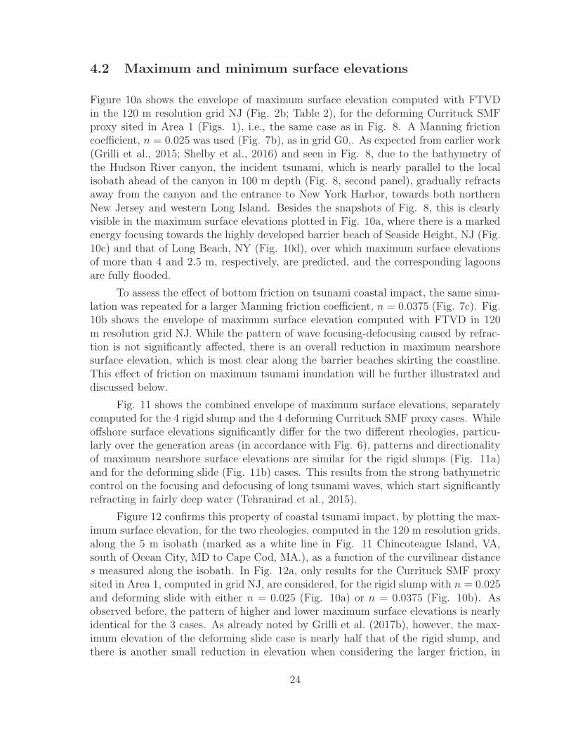
4.2 Maximum and minimum surface elevations

Figure 10a shows the envelope of maximum surface elevation computed with FTVDin the 120 m resolution grid NJ (Fig. 2b; Table 2), for the deforming Currituck SMFproxy sited in Area 1 (Figs. 1), i.e., the same case as in Fig. 8. A Manning frictioncoefficient, n = 0.025 was used (Fig. 7b), as in grid G0,. As expected from earlier work(Grilli et al., 2015; Shelby et al., 2016) and seen in Fig. 8, due to the bathymetry ofthe Hudson River canyon, the incident tsunami, which is nearly parallel to the localisobath ahead of the canyon in 100 m depth (Fig. 8, second panel), gradually refractsaway from the canyon and the entrance to New York Harbor, towards both northernNew Jersey and western Long Island. Besides the snapshots of Fig. 8, this is clearlyvisible in the maximum surface elevations plotted in Fig. 10a, where there is a markedenergy focusing towards the highly developed barrier beach of Seaside Height, NJ (Fig.10c) and that of Long Beach, NY (Fig. 10d), over which maximum surface elevationsof more than 4 and 2.5 m, respectively, are predicted, and the corresponding lagoonsare fully flooded.

To assess the effect of bottom friction on tsunami coastal impact, the same simu-lation was repeated for a larger Manning friction coefficient, n = 0.0375 (Fig. 7c). Fig.10b shows the envelope of maximum surface elevation computed with FTVD in 120m resolution grid NJ. While the pattern of wave focusing-defocusing caused by refrac-tion is not significantly affected, there is an overall reduction in maximum nearshoresurface elevation, which is most clear along the barrier beaches skirting the coastline.This effect of friction on maximum tsunami inundation will be further illustrated anddiscussed below.

Fig. 11 shows the combined envelope of maximum surface elevations, separatelycomputed for the 4 rigid slump and the 4 deforming Currituck SMF proxy cases. Whileoffshore surface elevations significantly differ for the two different rheologies, particu-larly over the generation areas (in accordance with Fig. 6), patterns and directionalityof maximum nearshore surface elevations are similar for the rigid slumps (Fig. 11a)and for the deforming slide (Fig. 11b) cases. This results from the strong bathymetriccontrol on the focusing and defocusing of long tsunami waves, which start significantlyrefracting in fairly deep water (Tehranirad et al., 2015).

Figure 12 confirms this property of coastal tsunami impact, by plotting the max-imum surface elevation, for the two rheologies, computed in the 120 m resolution grids,along the 5 m isobath (marked as a white line in Fig. 11 Chincoteague Island, VA,south of Ocean City, MD to Cape Cod, MA.), as a function of the curvilinear distances measured along the isobath. In Fig. 12a, only results for the Currituck SMF proxysited in Area 1, computed in grid NJ, are considered, for the rigid slump with n = 0.025and deforming slide with either n = 0.025 (Fig. 10a) or n = 0.0375 (Fig. 10b). Asobserved before, the pattern of higher and lower maximum surface elevations is nearlyidentical for the 3 cases. As already noted by Grilli et al. (2017b), however, the max-imum elevation of the deforming slide case is nearly half that of the rigid slump, andthere is another small reduction in elevation when considering the larger friction, in

24

the latter case. Figure 12b plots the same results at the 5 m isobath, but combined forall 4 Currituck SMF proxies sited in Areas 1-4, simulated in the 7 nested grids, andfor both rheologies (as in Fig. 11). Here the picture seems more complex, as we haveseen that all SMF sources can generate tsunamis that affect the entire upper USECin some manner, due to wave refraction over the complex geometry of the shelf break.While the rigid slumps still cause the maximum inundation, with 11.5 m around theeastern end of long Island near Montauk, NY (s = 800 km; Fig. 1), where the shelfbathymetry is particularly concave and causes high wave focusing, the reduction incoastal impact when considering deforming slides is overall less marked. For deformingslides, the maximum inundation is reduced to 8.5 m and now occurs near Atlantic City,NJ (s = 350 km; Fig. 1), while in Montauk the impact is reduced to 7 m. In thesecombined envelopes, the pattern of wave focusing and defocusing repeats itself, withthe lowest impact occurring in or near Bays and estuaries (e.g., Delaware Bay, NewYork harbor, Narragansett Bay, Buzzards Bay).

Finally, Fig. 12c shows the envelope of minimum surface elevations simulated atthe 5 m isobath, for the combination of the 4 Currituck SMF proxies sited in Areas1-4, simulated in the 7 nested grids, and for both rheologies. Such results would beimportant for instance when considering tsunami impact effects on the fresh waterintakes of a power plant, of which there are a few in this area (e.g., nuclear powerplants in Millstone, CT near the mouth of Long Island Sound or Oyster Creek, NJ,just south of Seaside Height). Here, results appear quite similar for the rigid slumpand deforming slide cases; at a few instances, in particular near Atlantic City (s = 350km) and Montauk (s = 800 km), the minimum elevation would reach down to theseafloor (i.e., 5 m; with some minor irregularities related to discretization and themoving shoreline algorithm). This similarity in minimum values is expected sincethe minimum coastal elevation is typically caused by the depression wave that firstarrives on the nearest shores facing Areas 1-4 (Figs. 1 and 9), and it is a result of theinitial motion of each SMF, i.e., at short time when deformation has not yet playedan important role, but instead SMF mass, initial acceleration, and local slope controlwave generation (Grilli and Watts, 2005).

5 Discussion and conclusions

In their probabilistic analysis (MCS) of landslide tsunami hazard along the USEC,Grilli et al. (2009) concluded that the 500 year tsunami runup along the upper USECwas largest from Virginia to Cape Cod (about 6-7 m maximum). Additional MCSand geotechnical analyses identified 4 areas (Fig. 1) where large SMFs were bothpossible due to large sediment accumulation and most probable due to low factorof safety in slope stability analyses (Krauss, 2011; Eggeling, 2012). In light of this,with the aim to simulate Probable Maximum Tsunamis (PMTs), Grilli et al. (2015)performed direct simulations for extreme SMFs having the lumped characteristics ofthe historical Currituck slide complex (i.e., “Currituck SMF proxies”; 30 km long by

25

20 m wide by 0.75 km maximum thickness), and to maximize coastal impact modeledthem as rigid slumps. The coastal inundation caused by these SMF tsunamis wascombined with that caused by other PMTs from extreme sources identified in theAtlantic Ocean (Grilli et al., 2010; Tehranirad et al., 2015; Grilli et al., 2017a), toproduce the first generation of tsunami inundation maps for the most exposed areasof the USEC to tsunami hazard, under the auspice of the National Tsunami HazardMitigation Program (NTHMP) (Tehranirad et al., 2014, 2015a,b,c,d,e). The presentstudy was performed in the context of this earlier work, as newer model simulatingdifferent slide rheologies became available (Kirby et al., 2016; Grilli et al., 2017b), andconsidering that all SMFs failed as rigid slump was being questioned as being perhapstoo conservative.

Thus, in this work, while still considering Currituck SMF proxies sited in Areas1-4 (with a 158 km3 volume), we performed new numerical simulations to assess howtsunami hazard along the upper US East Coast is affected by SMF rheology, i.e.,whether the SMFs behave as rigid slumps or deforming slides. Based on earlier work(Grilli et al., 2017b), the latter were assumed to have the same bulk density as rigidslumps (ρs = 1, 900 kg/m3), a fairly large viscosity in the upper range of debris flows(νs = 0.5 m/s2), and a substrate to slide Manning friction coefficient n = 0.1. Asthese simulations used higher resolution grids than before, and to perform a detailedcomparison, besides tsunami generation from deforming slides, we re-simulated tsunamigeneration for the rigid slumps considered by Grilli et al. (2015). In all cases, tsunamigeneration was simulated using the 3D non-hydrostatic model NHWAVE (for slumps)(Ma et al., 2012) and the two-layer NHWAVED model (for deforming slides) (Kirbyet al., 2016), and the initial SMF geometry was assumed to be quasi-Gaussian (belowcurrent seafloor) with an elliptical footprint on the slope. For rigid slumps, both timevarying geometry and law of motion were specified as bottom boundary conditions(Grilli and Watts, 2005; Watts et al., 2005; Grilli et al., 2015) and, for deformingslides, SMF motion and deformation were directly modeled in NHWAVED, as a depth-integrated bottom layer of dense Newtonian fluid, fully coupled to the overlying fluidmotion modeled with the standard σ-layer NHWAVE. Once the SMFs were no-longertsunamigenic (i.e., the slumps had stopped moving or the slides were deep and thinenough), we continued simulating tsunami propagation using the 2D fully nonlinear anddispersive long wave model FUNWAVE-TVD. For the onshore tsunami propagation,we use nested grids of 500 and 120 m resolution and applied our standard one-waycoupling methodology.

Results of tsunami generation simulations showed that deforming slides, whilehaving a slightly larger initial acceleration, generated smaller onshore propagatingtsunamis than rigid slumps, due to their spreading and thinning out during motion,which gradually makes them less tsunamigenic; by contrast, rigid slumps kept theirspecified shape during their pendulum-like motion. Also, since they flowed down theslope following the terrain, deforming slides caused more asymmetric tsunamis along-shore, with respect to their initial direction of motion, than rigid slumps (Fig. 5). Theoffshore-propagating tsunami waves were usually as large or larger than for slumps (Fig.

26

6). Effects of SMF rheology on coastal tsunami impact, were evaluated by comparingthe combined maximum envelope of surface elevation caused nearshore and along theshore over the 5 m isobath, by tsunamis generated by the 4 rigid slumps or deformingslides (Fig. 12). Consistent with earlier work (Tehranirad et al., 2015, 2017; Grilliet al., 2017b), we found that the bathymetry of the wide shelf has strong, first-order,control on the magnitude of tsunami coastal inundation, as it induces wave focusingand defocusing effects. Additionally, tsunami propagation and refraction over the shelf,both north and south of each source area, causes non-trivial variations in surface ele-vation and coastal inundation. This implies that a given SMF can generate tsunamiwaves that cause a significant coastal impact far alongshore from their source area.Overall, as expected from earlier work (Grilli and Watts, 2005; Grilli et al., 2017b),tsunamis caused by rigid slumps were found to be worst case scenarios, causing thelargest maximum inundation at all sites (with a maximum of about 11.5 m aroundMontauk, NY), and up to 50% more inundation than for the slides considered here,which had a moderate level of deformation. For rigid slumps, the maximum computedinundation of 8-11.5 m at the 5 m isobath is larger than the estimated 500 runup of 6-7m by Grilli et al. (2009), also based on rigid slumps (or slides) assumptions. This couldbe expected since the Currituck SMF proxies considered here were aimed at causingPMTs for the upper USEC, with potentially thousands of years return periods (the es-timated age of the Currituck slide complex is about 16Ka). By contrast, the maximuminundation of 8.5 m computed here for deforming slides (around Atlantic City) is moreconsistent with the 500 year runup estimated in earlier work based on MCS. This couldindicate that the return period of the largest events was underestimated in the MCSwork. Regarding minimum elevations at the coast, which affect power plant intakes,tsunamis from both types of SMFs were shown to be able to cause water withdrawalto the 5 m isobath or deeper. Finally, the effects of bottom friction on tsunami coastalinundation were assessed by performing simulations for the Area 1 deforming slide inthe 120 m NJ grid, using two different Manning coefficients, one 50% larger than theother. Using the increased friction from n = 0.025 to 0.375, led to a reduction ofthe largest tsunami inundations at the coast, in some cases, by up to 15%. Smallerinundation levels were less noticeably affected.

In conclusion, it seems that unless tsunami hazard assessment is performed for acritical coastal facility (such as a nuclear power plant), which requires considering themost extreme PMTs, it appears more realistic for standard tsunami hazard assessment(such as the NTHMP inundation mapping) to consider moderately deforming SMFs,whose center of mass follows a similar kinematics as that of the rigid slumps butwhose deformation leads to reduce coastal impact. This is also consistent with paleo-SMF observations made on the upper East coast continental shelf and margin (tenBrink et al., 2014). Considering its marked effect on maximum inundation, valuesof the bottom friction coefficient should be carefully selected, particularly nearshore.Additional nearshore simulations of coastal inundation, in high-resolution grids (e.g.,30 m), caused by the deforming slide PMTs will be left out for future work.

27

Acknowledgments

This work was supported by the National Tsunami Hazard Mitigation Program (NTHMP),NOAA, through Grants NA-15-NWS4670029 and NA-16-NWS4670034 to the Univer-sity of Delaware (with subaward to the University of Rhode Island). Additional sup-port at the University of Rhode Island and the University of Delaware came fromGrants CMMI-15-35568 and CMMI-15-37568 from the Engineering for Natural Haz-ards Program, National Science Foundation, respectively. Development of the numer-ical models used in this study was supported by the Office of Naval Research, LittoralGeosciences and Optics program. Finally, numerical simulations reported in this workused HPC resources as part of the Extreme Science and Engineering Discovery En-vironment (XSEDE), which is supported by the National Science Foundation grantnumber ACI-1548562.

References

Abadie S, Harris JC, Grilli ST and R Fabre (2012). Numerical modeling of tsunamiwaves generated by the flank collapse of the Cumbre Vieja Volcano (La Palma,Canary Islands) : tsunami source and near field effects. J Geophys Res, 117:C05030,doi:10.1029/2011JC007646.

Amante C and BW Eakins (2009). ETOPO1 1 Arc-Minute Global Relief Model: Proce-dures, Data Sources and Analysis. NOAA Technical Memorandum NESDIS NGDC-24. National Geophysical Data Center, NOAA. doi:10.7289/V5C8276M [March 15,2017].

ECMAP 2017. NTHMP tsunami inundation maps for the US East Coast.https://www.udel.edu/kirby/nthmp.html.

Eggeling T (2012). Analysis of earthquake triggered submarine landslides at four loca-tions along the U.S. east coast. Masters Thesis. University of Rhode Island.

Enet F, and ST Grilli (2007). Experimental Study of Tsunami Generation by Three-Dimensional Rigid Underwater Landslides. J. Waterway, Port, Coastal, Ocean Eng.133(6):442-454. doi: 10.1061/(ASCE)0733-950X(2007)133:6(442).

Fine I.V., Rabinovich AB, Bornhold BD, Thomson R and EA Kulikov (2005) TheGrand Banks landslide-generated tsunami of November 18, 1929: preliminary anal-ysis and numerical modeling. Mar Geol, 215:45-57.

Geist E, P Lynett and J Chaytor (2009). Hydrodynamic modeling of tsunamis from theCurrituck landslide. Marine Geology, 264:41-52, doi:10.1016/j.margeo.2008.09.005.

Glimsdal S, Pedersen GK, Harbitz CB and F Løvholt (2013). Dispersion oftsunamis: does it really matter ? Nat. Hazards Earth Syst. Sci., 13:1507-1526,doi:10.5194/nhess-13-1507-2013.

28

Grilli ST and P Watts (1999). Modeling of waves generated by a moving submergedbody. Applications to underwater landslides. Engng Analys Boundary Elements,23:645-656.

Grilli ST and PWatts (2005). Tsunami Generation by Submarine Mass Failure. I: Mod-eling, Experimental Validation, and Sensitivity Analyses. J. Waterway, Port, Coastal,Ocean Eng. 131(6):283-297. doi:10.1061/(ASCE)0733-950X(2005)131:6(283).

Grilli ST, Taylor O-DS, Baxter CDP and S Maretzki (2009). Probabilistic approachfor determining submarine landslide tsunami hazard along the upper East Coast ofthe United States. Mar Geol 264(1-2):74-97.

Grilli ST, Dubosq S, Pophet N, Perignon Y, Kirby JT and F Shi (2010). Numericalsimulation and first-order hazard analysis of large co-seismic tsunamis generatedin the Puerto Rico trench: near-field impact on the North shore of Puerto Ricoand far-field impact on the US East Coast. Nat Haz Earth Syst Sc, 10:2109-2125,doi:10.5194/nhess-2109-2010.

GrilliJ ST, Harris JC, Tappin DR, Masterlark T, Kirby JT, Shi F and G Ma (2012).Numerical modeling of coastal tsunami dissipation and impact. In Proc. 33rd Intl.Coastal Engng. Conf. (P. Lynett and J. Mc Kee Smith, eds.) (ICCE12, Santander,Spain, July, 2012), 12 pps. World Scientific Publishing Co. Pte. Ltd.

Grilli ST, Harris JC, Tajalibakhsh T, Masterlark TL, Kyriakopoulos C, Kirby JT andF Shi (2013). Numerical simulation of the 2011 Tohoku tsunami based on a newtransient FEM co-seismic source: Comparison to far- and near-field observations.Pure Appl. Geophys., 170:1333-1359, doi:10.1007/s00024-012-0528-y.

Grilli ST, O’Reilly C, Harris JC, Tajalli Bakhsh T, Tehranirad B, Banihashemi S, KirbyJT, Baxter CDP, Eggeling T, Ma G and F Shi (2015). Modeling of SMF tsunamihazard along the upper US East Coast: detailed impact around Ocean City, MD.Nat Hazards 76(2):705-746. doi:10.1007/s11069-014-1522-8.

Grilli ST, Grilli AR, Tehranirad B and JT Kirby (2017a). Modeling tsunami sourcesand their propagation in the Atlantic Ocean for coastal tsunami hazard assessmentand inundation mapping along the US East Coast. In Proc. Coastal Structures andSolutions to Coastal Disasters 2015 : Tsunamis (Boston, USA. September 9-11,2015), American Soc. Civil Eng., pps. 1-12.

Grilli ST, Shelby M, Kimmoun O, Dupont G, Nicolsky D, Ma G, Kirby JT and F Shi(2017b). Modeling coastal tsunami hazard from submarine mass failures: effect ofslide rheology, experimental validation, and case studies off the US East Coast. NatHazards 86(1),353-391. doi:10.1007/s11069-016-2692-3.

Hill JC, Brothers DS, Craig BK, Uri S, Chaytor JD and CH Flores (2017). Geo-logic controls on submarine slope failure along the central US Atlantic margin:

29

Insights from the Currituck Slide Complex. Marine Geology, 385:114-130. doi:10.1016/j.margeo.2016.10.007.

Kirby JT, Shi F, Tehranirad B, Harris JC and ST Grilli (2013). Dispersive tsunamiwaves in the ocean: Model equations and sensitivity to dispersion and Coriolis effects.Ocean Modell, 62:39-55, doi:10.1016/j.ocemod.2012.11.009.

Kirby JT, Shi F, Nicolsky D and S Misra (2016). The 27 April 1975 Kitimat, BritishColumbia submarine landslide tsunami: a comparison of modeling approaches.Landslides,13(6):1421-1434. doi: 10.1007/s10346-016-0682-x.

Krauss T (2011). Probabilistic tsunami hazard assessment for theUnited States East Coast. Masters Thesis. University of Rhode Island.http://chinacat.coastal.udel.edu/nthmp/krause-ms-uri11.pdf.

Locat J, Lee H, ten Brink US, Twitchell D, Geist E and M Sansoucy (2009). Geomor-phology, stability and mobility of the Currituck slide. Mar Geol 264:28-40.

Løvholt F, Pedersen G and G Gisler (2008). Oceanic propagation of a potential tsunamifrom the La Palma Island. J Geophys Res, 113:C09026.

Ma G, Shi F and JT Kirby (2012). Shock-capturing non-hydrostatic model for fullydispersive surface wave processes. Ocean Modell, 43-44:22-35.

Madsen PA, Fuhrman DR and HA Schaffer (2008). On the solitary wave paradigm fortsunamis. J Geophys Res, 113, C12012, 22 pp.

Matsuyama M, Ikeno M, Sakakiyama T and T Takeda (2007). A study of tsunamiwave fission in an undistorted experiment. Tsunami and Its Hazards in the Indianand Pacific Oceans. Pure Appl Geophys, 164:617-631.

National Geophysical Data Center (1999a). U.S. Coastal Relief Model - Northeast At-lantic. National Geophysical Data Center, NOAA. doi:10.7289/V5MS3QNZ [March15, 2017].

National Geophysical Data Center (1999b). U.S. Coastal Relief Model - SoutheastAtlantic. National Geophysical Data Center, NOAA. doi:10.7289/V53R0QR5 [March15, 2017].

Piper DJW, Cochonat P and ML Morrison (1999). The sequence of events around theepicentre of the 1929 Grand Banks earthquake: initiation of the debris flows andturbidity current inferred from side scan sonar. Sedimentology, 46:79-97.

SLIDE (2017). Slope Stability Analysis Model. RockScience Inc.https://www.rocscience.com/rocscience/products/slide.

Shelby, M, Grilli ST and AR Grilli (2016). Tsunami hazard assessment in the Hud-son River Estuary based on dynamic tsunami tide simulations. Pure Appl Geo-phys,173(12), 3,999-4,037, doi:10.1007/s00024-016-1315-y.

30

Shi F, Kirby JT, Harris JC, Geiman JD and ST Grilli (2012). A high-order adaptivetime-stepping TVD solver for Boussinesq modeling of breaking waves and coastalinundation. Ocean Modell, 43-44:36-51, doi:10.1016/j.ocemod.2011.12.004.

Tappin DR, Watts P and ST Grilli (2008). The Papua New Guinea tsunami of 1998:anatomy of a catastrophic event. Natural Hazards and Earth System Sciences, 8:243-266.

Tappin DR, Grilli ST, Harris JC, Geller RJ, Masterlark T, Kirby JT, F Shi,G Ma, Thingbaijamg KKS and PM Maig (2014). Did a submarine landslidecontribute to the 2011 Tohoku tsunami ? Marine Geology, 357:344-361 doi:10.1016/j.margeo.2014.09.043.

Tehranirad B, Banihashemi S, Kirby JT, Callahan JA and F Shi (2014). Tsunamiinundation mapping for Ocean City, MD NGDC DEM. Research Report No. CACR-14-04, Center for Applied Coastal Research, Department of Civil and EnvironmentalEngineering, University of Delaware.

Tehranirad B, Harris JC, Grilli AR, Grilli ST, Abadie S, Kirby JT and F Shi (2015).Far-field tsunami hazard in the north Atlantic basin from large scale flank collapsesof the Cumbre Vieja volcano, La Palma. Pure Appl Geophys, 172(12):3,589-3,616,doi:10.1007/s00024-015-1135-5.

Tehranirad B, Kirby JT, Callahan JA and F Shi (2015a). Tsunami inundation map-ping for Atlantic City, NJ NGDC DEM. Research Report No. CACR-15-01, Centerfor Applied Coastal Research, Department of Civil and Environmental Engineering,University of Delaware.

Tehranirad B, Kirby JT, Callahan JA and F Shi (2015b). Tsunami inundation mappingfor the northern half of the State of New Jersey. Research Report No. CACR-15-02, Center for Applied Coastal Research, Department of Civil and EnvironmentalEngineering, University of Delaware.

Tehranirad B, Kirby JT, Callahan JA and F Shi (2015c). Tsunami inundation map-ping for New York City. Research Report No. CACR-15-03, Center for AppliedCoastal Research, Department of Civil and Environmental Engineering, Universityof Delaware.

Tehranirad B, Kirby JT, Callahan JA and F Shi (2015d). Tsunami inundation map-ping for Montauk, NY NGDC DEM. Research Report No. CACR-15-04, Centerfor Applied Coastal Research, Department of Civil and Environmental Engineering,University of Delaware.

Tehranirad B, Kirby JT, Callahan JA and F Shi (2015e). Tsunami inundation map-ping for Nantucket, MA NGDC DEM. Research Report No. CACR-15-05, Centerfor Applied Coastal Research, Department of Civil and Environmental Engineering,University of Delaware.

31

Tehranirad B, Kirby JT, Grilli ST, Grilli AR and F. SHi (2017). Continental ShelfBathymetry Controls the Spatial Distribution of Tsunami Hazard for the US EastCoast. Geophys Res Lett (in preparation).

ten Brink, U, Twichell D, Geist E, Chaytor J, Locat J, Lee H, Buczkowski B, Barkan R,Solow A, Andrews B, Parsons T, Lynett P, Lin J, and M Sansoucy (2008). Evaluationof tsunami sources with the potential to impact the U.S. Atlantic and Gulf coasts.USGS Administrative report to the U.S. Nuclear Regulatory Commission, 300 pp.

ten Brink US, Lee HJ, Geist EL and D Twichell (2009a) Assessment of tsunami haz-ard to the U.S. East Coast using relationships between submarine landslides andearthquakes. Mar Geol, 264:65-73.

ten Brink US, Barkan R, Andrews BD and JD Chaytor (2009b) Size distributions andfailure initiation of submarine and subaerial landslides. Earth Planetary Sci Lett,287:31-42.

ten Brink US, Chaytor JD, Geist EL, Brothers DS and BD Andrews (2014) Assessmentof tsunami hazard to the U.S. Atlantic margin. Mar Geol, 353:31-54.

Towns J, Cockerill T, Dahan M, Foster I, Gaither K, Grimshaw A, Hazlewood V,Lathrop S, Lifka D, Peterson GD, Roskies R, Scott JR and N Wilkins-Diehr (2014).XSEDE: Accelerating Scientific Discovery. Computing in Science and Engineering16(5):62-74. doi:10.1109/MCSE.2014.80.

Watts P, Grilli ST, Tappin DR and G Fryer (2005). Tsunami generation by submarinemass failure, II: Predictive equations and case studies. J Waterw Port Coast OcEngng, 131(6):298-310.

A SMF geometry and slump law of motion

For rigid slumps, kinematics is specified based on the analytical laws developed byGrilli and Watts (1999, 2005); Watts et al. (2005). Additionally, as in Enet and Grilli(2007), the SMF geometry is idealized as having a “Quasi-Gaussian” shape (belowseafloor) of elevation ζ(x, y), whose steepness is controlled by a shape parameter ε(here ε = 0.717), and elliptical footprint of downslope length b, width w, and maximumthickness T defined as (Fig. 13),

ζ(x, y) =T

1− εmax{0, sech(kbξ) sech(kwχ)− ε} (1)

where (ξ, χ) are the local downslope and spanwise horizontal coordinates, rotated inthe direction of SMF motion θ, and kb = 2C/b, kw = 2C/w, with C = acosh(1/ε).With this geometry and parameters, the SMF volume is given by,

Vs = bwTI2C2

( I1I2− ε

1− ε

)

with I1;2 =

∫ C

0

f(µ) dµ; g(µ) dµ (2)

32

and,

f(µ) = sechµ atan(sinh g(µ)) , g(µ) = acosh

(

sechµ

ε

)

(3)

[Note that Eqs. (2) and (3) have been corrected and are different from those reportedin earlier papers (e.g., Enet and Grilli (2007); Grilli et al. (2015)), which resultedfrom a mistake in the volume calculation.] For the specified ε, we find, C = 0.8616,I1 = 0.4804, I2 = 0.5672, and Vs = 0.3508 bwT .

Earlier modeling work (Locat et al., 2009) indicates that, during its tsunamigenicperiod of motion, the Currituck SMF achieved a relatively small maximum displace-ment (runout) Sf < b in its main direction of motion down the slope, over an unknowntime of motion tf . The combination of rigid block SMF and small displacement parallelto the slope supports modeling the SMF kinematics as a rigid slump or a deformingslide with moderate deformation achieving a similar runout over the same time. Ineither cases, one can assume a constant basal friction (i.e., slide to substrate friction)and negligible hydrodynamic drag (Grilli and Watts, 2005). This type of rigid-bodymotion kinematics was investigated in earlier work (see above-listed references), lead-ing for the slump to a pendulum-like center of mass motion S(t) parallel to the localmean slope of angle α. Here, we use this simple law of motion for rigid slumps, whichreads,

S(t) = S0

(

1− cost

t0

)

for 0 ≤ t ≤ tf (4)

with S0 = Sf/2 and t0 = tf/π, and S = Sf for t > tf (assuming SMF triggering occursat t = 0).

At t = 0, the SMF elevation is specified below the current seafloor bathymetryh0(x, y). Given the SMF initial center of mass location (x0, y0) in global axes (x, y) (i.e.,coordinates of the center of the elliptical footprint) and azimuth angle of SMF motionθ, we define the coordinate transformation to the local SMF slope-parallel coordinatesystem (ξ, χ) (Fig. 13) as,

ξ = (x− xo) cos θ − (y − y0) sin θ − S(t) cosα (5)

χ = (x− xo) sin θ + (y − y0) cos θ

with S(t) given by Eq. (4).

Then, assuming sinα ≃ 0 for small slopes, the instantaneous seafloor depth abovethe SMF is given by,

h(x, y, t) = h0(x, y) + ζ{ξ(x, y, t), χ(x, y, t)} − ζ{ξ(x, y, 0), χ(x, y, 0)} (6)

with ∆h = h − h0. The seafloor motion described by Eq. (6) is similar to a transla-tion parallel to the average slope of part of the seabed, over the actual bathymetry.The vertical seafloor velocity (used in NHWAVE as a bottom boundary condition) iscomputed as,

dh

dt(x, y, t) =

dζ

dt{ξ(x, y, S(t)), χ(x, y, t)} (7)

33

Figure 13: Geometric parameterization of a SMF initially centered at (x0, y0) movingin direction ξ, with an azimuth angle θ from North and center of mass motion S(t)measured parallel to the mean local slope of angle α; (x, y) denote the longitudinal andlatitudinal horizontal directions, respectively.

which can be easily derived from Eqs. (1) to (6) as,

dh

dt(x, y, t) = kb cosα

(

ζ +εT

1− ε

)

U tanh(kbξ) with U(t) =dS

dt= Umax sin

t

t0(8)

the slump velocity obtained from Eq. (4), with Umax = S0/t0 the maximum velocity.Similarly, the slump acceleration is found as,

A(t) =d2S

dt2= A0 cos

t

t0with A0 =

S0

t20(9)

the initial acceleration.

For rigid slumps, hydrodynamic drag can be neglected due to low velocity andsmall amplitude of motion, and inertia includes both the SMF mass Ms = ρsVs, with ρsdenoting the sediment bulk density, and the specific density being defined as γ = ρs/ρw,with ρw the water density, and an added mass ∆Ms = CMρwVs, defined by way ofan added mass coefficient CM . Assuming a constant basal friction, a nearly circularrupture surface of radius R, and a small angular displacement ∆Φ, Grilli and Watts(2005) derived the characteristic distance and time of motion for rigid slumps as,

S0 =R∆Φ

2and t0 =

√

R

g

γ + CM

γ − 1with R ≃

b2

8T(10)

with g denoting the gravitational acceleration. The last equation (10), proposed byWatts et al. (2005), is a semi-empirical relationship to estimate the radius of slumpmotion as a function of slump downslope length and maximum thickness.

34