voI-. 76, NO. 20 TOURNAL OF GEOPHYSIC,{L RESEARCH JULY 10, 1971

Earth's Gravity Field to the Sixteenth Degree and StationCoordinates from Satellite and Terrestrial Data

E. M. GeposcnKrN ¿,No K. LeMsncrl

Srnithson:ion Institutinn, Astrophysical ObseruatoryCambridge, Massachusetts 02138

Geodetic parameters describing the eárth's gravity field and the positions of satellite-tracking stations in a geocentric reference frame have been computed. These pârameterswere estimated by means of a combination of four different types of data: routine andsimultaneous satellite observations, observations of deep-space probes, and measurements ofterrestrial gravity. This combination solution gives beüter parametes than any subset ofdata types. In the dynamic solution, precision-reduced Baker-Nunn observations and laserrange data of 21 satellites were used. Data f¡om optical cameras, in addition to those from19 Baker-Nunn stations, were used in the geometúcal solution. Data from the tracking ofdeep-space probes were used in the form of relative station trongitudes and distances to theearth's axis of rotation. The surface-gravity data in the form of mean anomalies for 300-n.mi.squares were provided by Kaula. The adopted solution f¡om each iteration 'lvas a combina-tion solution and was chosen to improve the ¡esiduais of all types of dat¿. In addition tothese four data sets, astrogeodetic data, surface triangulaticn, and some recently acquiredsurface-gravity data not included in the set used for the combinations were used for an inde-pendent test of the solution. The total gravily field is represented by spherical harmoniccoeffcients complete to degree and order 16, plus a number of higherdegree terms. Thehalf-wavelength resolution of this global solution subtends about 11' at the earth's center.The accuracy of the global field has been estimated as -+3 meters in geoid height, or -r-8.7mgal. Coordinates of many of ühe stations are determined with an accuracy of l0 meters orbetter.

During 1966, the Smithsonia¡ AstrophysicalObservatorf (SAO) published numerical pa-rameters for the earth's gravity field and thecoordinates of the satellite-tracking stations

lGøposchlcin, 1967 ; Köhnlein, 1967 a; Veis,I9õ7a, b;

'Whipple, 7967; Lundquist ønd Veis,

19661. In 1967, a series of pap€rs by Gaposch-kin, Köhnlein, Kozai, and Veis lLw'dquist,19671 produced several refinements of the 1966soiution. Tests of the solution presented hereindicate that these new results are superior to.any set of geodetic parameters.

The geodetic parameters are estimâted froma combined solution of the results obtained bythe geometric and dynamic methods. In addi-tion, the combination solution includes station-position information deterrrined by the JetPropulsion Laboratory (JPt) for its DeepSpace Tracking Network (DSN) ând surface-gravity anomalies computed by KøuIø 1196641 .

'Now at Observafoire de Paris, Meudon, France.

Copyright @ 1971 by the American GçoPhysical Union.

The final solution yields harmonic coefficients in'the potential expansion compiete to degree andorder 16, plus 14 pairs of higher-degree coeffi-cients and the coordinates for 39 stations. Thissoiution is compared with recently av¿iÌablesurface-gravity data and astrogeodetic data.

D¿r¿ Cor.¿rcrroN, REDucrroN,exo Rp¡,onpwcE SysrEM

Dato, collection. Laser tracki¡g systems havebeen developed in the past 4 years, and coordi-nated observing periods were established in1967, 1968, and 1969. The best data includesignificant amounts of laser data.

In addition to data from the Baker-Nunn andlaser networks, data coilected by other agencieshave also been used (see Figure 1):

1. Laser data from stations 7815, 7816, and7818 were made available by the Centre Na- '

tional d'Etudes Spatiales (CNES), France.2. Laser clata from st¿tion 7050 were made

available by the Goddard Space Flight Center(GSFC).

4855

ei l íLro3qj

47r2^ 79459O8uA. .9O66e 9077

oa

oA

SÏATION POSITIONS DETERMINED BY

STATION POSITIONS DETERMINEO BY

STATION POS!TIONS DETERMINED 8Y

JPL POSTTIONS USED IN COMBINATION

Fig. 1. Location of stations

u

OYNAMIC AND GEOMETRIC SOLUTIONS

6EOMETRIC SOLUTION

DYNAMIC SOLUTION

'E0oC,r

used. Collocated stations are bracketed together.

Þ

EFzz

H

Ktd

x

\

E¿nrrr's Gn¿v¡rv F¡uLo ¿No Sterro¡r Coonnr¡r¡tss

3. Optical data were obtained from the fol-lowing European stations: 8015 a¡d 8019 (Ob-servatoire de Paris); 9065 (Technical Univer-sity of Delft) ; 9066 (Asironomical ïnstitute,Berne) ; 9074 and 9077 (USSR AstronomicalCouncil) ; and 9080 (Royai Radar Establish-ment, Malvern).

4. Optical data from the MOTS cameras1021, 1030, L042, 7036, 7037, 7039, 7040, 7075,and 7076 were supplied by GSFC.

.Datø red,uction and ø,ccurøci,es. The opticaldata were reduced with all terms in precessionand nutation necessary to ensure that the max-imum neglected effect is less than 0.5 meters.Annual aberration is added and diurnal aber-ration must be applied to the simultaneous ob-seryations. Parailactic refraction was applied bythe use of mean nighttime temperature and pres-sure taken at each station to establish therefraction coefficient (G. Veis, private com-munication, 1966). Systematic corrections tostar-catalog positions were applied where ap-propriate. AII optical data received from otheragencies were corrected in the same way. Theaccurâcy of the optical data ranges from 1 to 4a.rcsec lLømbeclc, 7969a].

The laser range data are considered to beaccurate to about 2 meters and are reduced byuse of the corrections described by Lehr [1969].The influencs 6f timing errors at the stationshas !o be'considered. For passes with more than10 observed points, 10 points equally spaced ilthe pass are selected. To account for redun-dancy and systematic errors of the iaser data,the assumed accuracy of each laser point istaken at 5 meters for the SAO and GSFC laserdata and at 10 meters for the CNES data.

Reference systern. SAO has its own masterclock, and through VLF transmission mai¡tainsits own coordinated time system called A.S. Theprincipal time reductions lrere to convert theGSFC data from UTC to A.S;, and the CNESdata from A3 to A.S. The UTl data used in1966 were a combination of final and prelimi-nary vaiues of the United States Naval Observa-tory (USNO). A¡ exami¡ation of the differencesbetween the USNO values and those of theBureau International de l'Heure (BIH) revealeddi.fferences approaching 5 meters. For the pres-ent solution, BIH UT1 values have been adoptedthroughout. It appears that these data may bea limiting factor for the ultimateþ attainable

4857

accuracy of station positions. The polar-motiondata were taken from the International PoiarMotion Service (IPMS). The difference betweenthese and the BIH data for the period since theywere referred to the same origin is as much as1.5 meters. The IPIVÍS data used here were allreferred to the mean pole of i900-1905. Thecoordinate system used is the equator of dateand the equinox of 1950.0. The choice of thissystem is discussed further in the next section.The position of the earth with respect to thissystem was tabulated i¡ terms of the UTl andpoiar-motion data.

As in 1966, the determination of the zonalharmonics wâs a precursor to this anaiysis.With use of the 1966 soiution, the orbital i¡for-mation was completely revised. Kozøi's ll969fzonal harmonics to /o were used as startingvalues. The coefficients are listed for referencein Table 1. AIso given are the adopted valueslor GM, ø", and the velocity of light c.

DYN¿urc¿r, Sor,utro¡r

The main problem in celestial mechanics is tpdevelop formulas (a theory in this nomencla-ture) that predict the trajectory when the forces

¿nd the initial conditions are established. In

TABLE 1. Adopted Zonal lIa¡monics to .I(21)*'and Other Constants

J(2)J(3)J(4)J(5).r(6)J(7)J(8)"r(e)"r(10),/(11)J(12)J(13)J(14).r(15)"r(16)J(r7)"r(18).r(1e)J(20)J(21)

GM B.gg60LB ! 1Q2o s6r/ssçza. 6.378155 X 108 metersc 2.997925 X 1010 cmlsec

1.08262800F-03-2.53808-06-1.5930846-2.3000F-07

5.0200E-07-3.6200F-07-1.1800E47-1.0000E-07-3.5400F-07

2.0200E-07-4.2000F-08-1.23008-07-7.30008{8-1.7400F-07

1.8700F-078.5000E{8

-2.31008-07-2.1600E{7-5.0000F-09

1.44008{7

* Rozai, 1969.

4858 Geposc¡rxr¡r e¡ro Le¡¿sncrgeneral, we must be satisûed with approximatesoiutions, rvhich for our purpose are quite satis_factory. Alternatively, a diiect numeìical inte_gration of the equations of motion could becarried out.

The forces we consider are the sravitationalattraction of the earth, moon, and sun and thenongravitational effects of radiation pressureand air drag. In this analysis, we havJ chosensatellites that are dominated by the geopoten-tial and for which othe¡ effects .uo,-ir, ,oor.way, be assumed. Kauta l1g66bl and, Gaposch_kin l1966al describe detailed methods for orbi_tal analysis. Gøposchlcin 11g6gl discusses someconsiderations of this anaiysis, and further de_tails are given by Gaposchlcín ønd Lotnbeclc[1e70] .

, The gravity field of the earth, or equivalently,the geopotential, is quite irregula".- The eeå_potential V can be represented. as an infi-niteseries of spherical harmonics, and the formadopted for this analysis is

' (C¡- cos øiÀ f S¿-. io -x)- l (1)- l "

where'GM is the product of the gravitationalconstant and the mass of the earth, $ and Àare earth-fixed latitude and longitude, @" i¡ theequatorial radius of the earth, and

p"(sín {)

2 / c ) ! s i n i - ' r

expression P¡- (sin þ) is ihe fully normalizedassociated Legendre pol¡nomial, i.e.,

* l l " o": n* m#oI p,^'(ri., ó){tind s p b e ¡ o ( C O S

: 11 [ i-)' kt (" - k)t (n - 2h)t

where r is the greatest itteger 1nf Z,

P¡-(sin ó)

: læl+lp-ø1,,, "o", ôL (¿ * rn)t _J z'

( 2 1 - z k ) r s ; r , j - m - 2 h

@

and C¿^,-S¿- are fully normalized. coefrcients, aspreviously published (sometimes designated asCr^, Sr^). The. p" (sin d) are the conventionalT¿egendre polynomials, and the Jo are convetr_tional harmonics. To include the,r" in the fullynormalized form, we have

P t , o : ( 2 1 * r ) " ' p ,

C ¿ , 0 : _ J I / ( L T + L ) " '

and the summation in equation 1 wouid be* - 0 ,7 ,2 , . . . , l . The Cr * , S r ^ a re ca l l edtesseral harmonics, and the ,/* are cajled zonalharmonics. For a systematic development, seeHeislcanen ond Moritz fig67l .

. fn equation 1, we assume Ji = C^ = S, : 0because the origin of the coordinate systemchosen is referred to the earth,s center of ïass,and the e axis (þ = o/2) is along the principalaxis, i.e., the axis of maximum moLent ofinertia. fn fact, these are only assumptions andone can only approximately realize such a co_ordinate system.

The tesseral harmonics are determined fromtheshort-period (1 revolution'to 1 day) changesin the orbit. The detailed structure oi tlr. orËitmust be observed, and each observation pro_vides an obse¡vation equation. Data of the hiEh_est possible precision are needed.

Apart from the resonant harmonics, the termshigher than I = 12, m = 12 are weaklv deter_mined by the satellite data (when the satelliteis low, it is infrequently observed), bui it haobeen demonstrated in early iterations that thesurface gravity could determine these hieherharmonics. The satellite solution was limiteã tothose harmonics that have an effect of qreaterthan 3 to 4 meters on the orbit. The re-sultingterms were complete through I - L2, m - ll,gpil l irg C/S(It, Z), C/S(r2,6), and C/502:,9). Higher-order terms selected were C/S(I, l)'i3 < ¿ < 16; C/S( t ,2) 18 < ¿ ( 15;!1!tt+, 3); c/SQ, 12) 18 < ¿ < ts;V/S(í,13) 13 < ¿ < 2I; C/S(t,r4) 14 < ¿ < 22'.The m = 9, 12, 13, 14 terms ,r" ,..on"ot *ithsome satellites. Gaposchlcin and Lambeclc lIgZ0.Tahle 4l iíst the resonant satellites wiih theii

v:w[ ' -å n f t ) "n^Gnø)

+ Ë å (î)'",-o*r,

(2- -

. 5- r-r¡

where r is the greatest integer <(¿ _ nx)/Z.Expression I uses a mixed normaiization. ihe

resonant periods. Several satellites are resonantwith more than one order. The stations rvererestricted to those observing many satellites.Other stations were more appropriately deter-mined by the geometric solution.

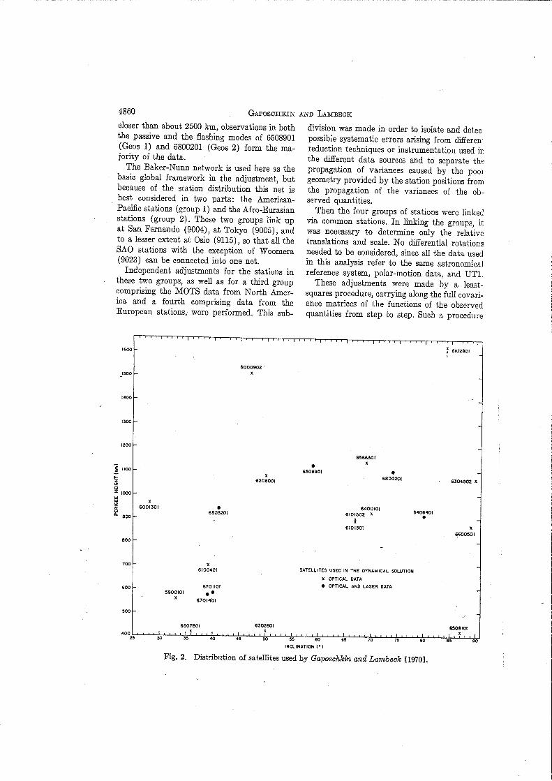
Table 2 details the selection of satellites usedin the final solution, ordered by inclination.Figure 2 indicates the distribution of satellites,many of which were not used in the 1966 solu-tion. The selection of data and unknownsevolved through the analysis. The number ofsatellites used ranged from 21 to 25, and thenumber of arcs in the largest solution was 244.Arcs were added and rejected on the basis ofcontribution to the normal equations, numberof observations for a particular station, im-provement of distribution for a resonant har-monic, and quality of the orbital fit.

Gpounrnrc Sor,urro¡r

The geometric method for determining sta-tion positions from observations of satellitesdoes not'require any knowledge of the orbit,since the object is observed simultaneously fromtwo or more stations and the reiative posi-tions of these stations are computed bv athree-dimensional triangulation pìo.u.r.'Thugeometric solution does not give any information

4859

on the position of the earth's center of mass,nor does it give a scale determination if onlydirection observations are used. The solutionis further characterized by highìy accuratedirections between stations, but also by anunfavorable error propagâtion in station coordi-nates. When combined with the dynamic solu-tion, the geometric solution contributes signifi-cantly to the solution for station coordinatesand provides a valuable means of assessing tltereliability of these results.

A total of 38 stations was involved in thissolution, and 20 of these were âlso used in thedyna.mic solution. Observations from 1ô SAOand 4 United States Air Force (USAF) Baker-Nunn cameras, from 13 National Aeronauticsand Space Admi¡istration (NASA) IVIOTScameras, and from 7 European stations wereutilized. Approximately 50,000 individual direc-tion observations were used in the analysis, anumber comparable to that used in the dy-namic solution. The distribution of the dataâ,mong lhe stations is given by Gaposchkin andLarnbeck [1970, Table 6]. Most of the observa-tions have been made to high-altitude satellitesnot used in the dynamic solution. These satel-iites inciude 610280i (Midas 4), 6303004,6605601 (Pageos), and 6805501. For stations

EeRrrt's Gnevrry Frpr,o ¿No Sr¿uo¡¡ CoonorN¿rns

TABLE 2. Summary of Dynamical Data

Name o¡ Other f¡cliuation,Designation deg

Semimajor PerigeeAxis, Height,

Ecce¡t¡icity km kmNew Select Læe¡

Days/Arc S¿tellite Files DatsNumberof .A.¡cs

600f301 Couier 18 60 yl

5900101 Yanguard 2 59 cl6100401 61 ô16701401 DrD6701101 DlC6503201 Erplorer 27 BE-C6000902 60 ú26206001 Änna 18 62 Fpl6302601 GeophysicalResearch650890f Exp.lorer 29 Geos I6101501 T¡amit 4.A. 6l ol6101502 Injun I 67 oZ6506301 Seco¡ õ6400r016406401 Explorer 22 BE-B6508101 Ogo 26600501 Osc¿¡ 076304902 5BN-26102801 Midæ 4 61 ¿ðl6800201 Explorer 36 Geoe 26õ0780r ov1 2

28

3939404L

õ05059o t

o t

69708087899098

r06144

0 .0160 . 1650 . 1190.053o .0520.0260 .0110.0070 .062o.0730.0080.0080.079o.0020 .0120 .0750 .0230.0050 .0 r3.0 .0310.182

7465 9658300 5577960 7007337 5697336 5797311 9417971 15727508 70777237 4248074 772L7318 8857316 8968159 7737730t 9217362 gtz7344 420v4r7 8687473 1070

10005 35037709 1101830ô 416

XXX

XX

XXX

X

x

XXX

XXXXXX

XX

6 3 0

a 1 ^

6 1 44 1 44 3 07 3 0

72 306 1 4

21 308 3 04 3 02 3 03 3 02 3 02 1 4r 3 05 3 03 5 00 1 42 1 4

4860 Geposc¡*rN ¿No L¿l¡npcr

close¡ than about 2500 lm., observations in boththe passive and the flashing modes of 650g901(Geos 1) and 6800201 (Geos 2) form the ma-jority of the data.

The Baker-Nunn network is used here as thebasic global framework in the adjustment, butbecause of the station dist¡ibution this net isbest considered in two paris: the American-Paciûc stations (group 1) and the Afro-Eurasianstations (group 2). These two groups link upat San Fernando (9004), at Tokyo (9005), andto a lesser ertent at Oslo (9115), so that all theSAO stations with the exception of

'W'oomera

(9023) can be connected irrto one net.Independent adjustments for the stations in

these two groups, as well as for a third groupcomprisilg the MOTS data from North Amer-ica and a fourth comprising data from theEuropean stations, were performed. This sub-

division was made in order to isolate and detecrpossible systematic errors arising from clifferenrreduction techniques or i¡strumentation used inthe djfferent data sources and to separate thepropagation .of variances caused by the poorgeometry provided by the station positions fronthe propagation of the variances of the ob_served quantities.

Then the four groups of stations were linkeclvia common stations, la linkì¡g the groups, itwâs necessary to determine only the reiativetranslations and scale. No di-fferential rotationsneeded to be considered, since all the data useclin this analysis refer to the same astronomicalreference system, polar-motion data, and. UT1.

These adjustments were made by a least-squares procedure, carryiag along the full covari-ance matrices of the functions of the observedquantities from step to step. Such a procedure

E

I

À

t x c L Ñ Â t t o N t . I

Fig. 2. Distribution of satellites used by Gaposchlcí,n and, Larnbeck lLg.¿01.

e400tol6tolSoz x 6406{0l

T .6 r 0 r 5 0 t x

6600501

SÂfELLITES USEO IN THE OYT¡ÄMICAL SOLUTTON

x oPncÂL 0ÁTA

. OPTICÀL ÁÈO LASER OAfA

\ .

\

\

\\

, - \

N

E t o

{

N <

b+

N >b

Ôl

is equivalent to adjusting ail the data in asingle step lTimstrø, 1956; Baarda, 19671, buiit has the advantage of isolating possible syste-matic errors in the data. If statisticai testingof the results indicated the presence of sucherrors, the adjustments were further split upin an attempt to locate the faulty data. Thestatistical testing procedures used followed theideas of Bøørda [i968].

Throughout the adjustment, it has been as-sumed that observations t¿ken at different timeinstants or from different stations are uncorre-lated. Systematic timing errors may prevailover a long period, so that the first assurmptionis difficult to justify. The second assumption,however, appears generally acceptable, sinceerror in time kept at distant stations is almostahvays uncorrelated. An anaiysis of the resultsof the adjustment of the various steps will

4861

indicate whetl.rer or not these assumptions arevalid.

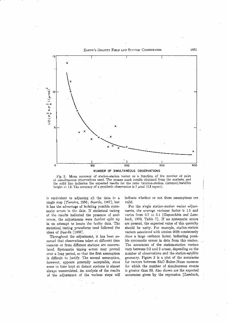
For the single station-station vector adjust-ments, the ,averâge variance factor is 1.5 andvaries from 0.7 to 3.1 lGøposchkin ørd Løm-beck, 1970, Table 71 . If no systematic errorsare present, the expected value of this quantityshould be unity. For example, station-stationvectors associated with' station 9028 consistentlyshow a large variance factor, i:rdicating possi-ble systematic errors in data from this station.Thé accuracies of the station-station vectorsvary between 0.2 and 2 arcsec, depending on thenumber of observations and the station-satellitegeometry. Figure 3 is a plot of the accuraciesfor vectors between SAO Baker-Nunn camerasfor which the mrmber of simultaneous eventsis greater than 30. Also shown are the expectedaccuracies given by the expression lLambeclc,

Eenr¡r's Gnlvrrr Frnr,o ¿Np Sr¿tro¡¡ CoonptN¿tps

NUMBER OF SIMULTANEOUS OESERVATIONS

Fig. 3. Mean accure,cy of staüion-station vector as a funcfion of the number of pairsol simultaneous observations used. The crosses mark results obtained from the analysis, andthe solid line indicates the expected resuits for the ratio (station-station disiance)/satelliteheight : 12. The accuracy of a synthetic observation is 7 prad (1.5 alcsec).

4862

1969ölG¡posc¡rxrw ¿No Lervrsucr

rvhere ou is the accuracy of a synthetic obser-vation (1.5 arcsec), and L/h is the average

. ratio of length of station-station vector to satel-i i te height (=1.2); øo is the accuracy in thevertical component, and o, is the accuracv inthe azimuth component of the station-staìionvector, and generally the correlation betweenthese components is small.

The variances of unit weight for the adjust_ment in the second phase of the four groups ofstations are the following:

group I o] : L.39 (Baker-Nunn, Americas,Pacific, Atlantic).

group 2 oz2 : L.59 (Baker-Nunn, Afro-Eurasian).

group 3 øsz : 0.93 (European Optical).group 4 a¿2 : 1.99 (North American MOTS).

'Appìication of the variance ratio tests to the

results leads to the general conclusion that, withthe exception of the data in group B, the nullhypothesis (i.e., there a¡e no model errors) is tobe rejected. However, a ¡eevaluation of the orie-inal data gave no indication where the orob-lems may occur, and the results have, of neces-sity, been accepted.

Finally, the adjustment linking the fourgroups of data gives a variance of unit weiEhtequal to 1.4 with 16 degrees of freedom and/0.*,,,,, : 1.71. This suggests that the observa-tions and methods of reduction used in the fourgroups are compatible.

To investigate further the unsatisfactory con-clusions that have to be dr¿wn from tho inde-pendent group adjustments, the directions be-tween stations were computed from the linkedadjustment results and were compared with theindependent group station-station vectors (seeGaposchlcin ønd, Lømbeck lI9T0, Figure 4lfor some exarnples). Both these vectors repre-sent estimates of the same quantity, and theycan be expected to lie within the accuracy esti-mates given for them. Comparisons for all thestation-station vectors show that this is thecâse âbout 60% of. the time.

Denoting the mean accuracy of a station-station vector derived from phase 1 by ø1 and

that derived from phase B by ø., and denotinrthe angular distance between the two estimate.of the vector by 8, we would expect that o¡the average

õ ' z < ( r / 2 ) ( 6 , ' + o , " )

These quantities are given by Gaposchkin antlLambeclc [1970, Table Z], and their values,averaged over the vectors used, indicate thatthis condition is not satisfied unless the varianceestimates are multiplied by a factor

Ie, : ,* ô2

,,, ò@7 + o":)These results yietd a value of Æ' = 2.8, andthe covariance matrix for the final seometricsolution is muliiptied by ihis number. The finaldirections between stations are given by Ga-poschldn and Lambeclc [1970, Table 8].

Ixronu¿rro¡q rRoryr Dnnp-Spacu pnosrs

The DSN has used data from its trackinE ofdeep-space probes to obtain_among other pa-rameters, the relative longitudes and the dis_tances to the earth's axis of rotation of theirantennas lVegos and Traslc, Ig6Z; Troslc ond,Vegos; Ig68l. As the JPL sites can be rel¿tedto nearby Baker-Nunn sites, by use of ground_survey information, a vajuable and completelvindependent control of the results is póssible.Comparison with the JPL data is pariicuhrlvimportant for the two instanceÉ where the eeo-met¡ic solution is either very poor (SoutirAfrica) or nonexistent (Australia). The twosets of data also complement each other, sincethe JPL solution gives a very strong scale andrelative longitude deterrnination but no latitudeinformation, whereas ihe SAO solution accu-rateiy determines the orientation with respectto the astronomical reference system.

The JPL and SAO results were compared bv7ø's [1966] and. Vegos and, Traslc flgtiZi usingdata from the Ranger missions. However, morãrefined JPL solutions have recently becomeavailable using data from the Mariner 4 and 5missions. The solution used in the present anal-ysis is that of. Mottinger [1969], caled LS 25.Table 3 gives his determination for the stationlocations. Mottinger estimates the standarddeviations of the computed quantities to be¿bout 3 meters. In this solution, the poiar-

l";l :',' lt/to'os(¿/å) - o.oalllon') " lt/lo.z+(L/h) - o.15l.]

Eenru'g Gn¡vrrr Frnr,o ¿Np Stetrow Coono¡N¿t¡s

TABLE 3. Locations of the JPL Antennas*

4863

Station tr, deg r", km X, km l, km

^ 4 1 ,

474t

47514767

243.194'Ð59136 .887507148 .98130127 .685432

355 .751007

õ212.0i,3-o5450. 19865205 .3ã045742.94174862 .6078

-2350.4397-3978.7174-4460.9809

5085.44254849.2429

-46ã1 .98193724.845+2682.40972668 .2678

- 360.2752

* Determined by Mottinger 11969l-

motion data from BIH and UTl derived fromUSNO data are used. Thus, a difference in longi-tude between the JPL and the SAO solutioncân be eKpected. A longitude difference canalso arise from possible discrepancies in theright-ascension definitions of the planetary

ephemeris used by JPL and of the star catalogused at SAO.

The geodetic coordinates of the JPL and asso-ciated Baker-Nunn stations are given by

Gaposchlû,n ønd Lømbeclc 11970, Table 101 . Inthree cases, 9002-4751 (South Africa), 9003-4741 (Australia), and 91134712 (Uniied

States), the survey distance between the sta-tions is small and any datum tilts or distor-tions should not, cause probiems when the geo-

detic survey information is used to relate the

two earth-centered systems. However, for the

other two JPL-SAO station groups, 90034742and 9004-4761, this may not be true, and cor-

rected s'urvey differences h¿ve been computedon the basis of the datum adjustments of the

European and Australian datums lLambøch,7970, 197ral.

Sunr¡cP-GneurY Derl

Surface-gravity data provide a means of com-

paring the satellite solution with an erternal

standard and of improving the over-all gravity-

freld solution. The satellite solutions are most

suited for determining the lower-order har-

monics, while the surface-gravity data are ex-

pected to contribute most to the higher-order

ierms. The dynamic satellite solution described

above gives a complete representation to degree

and order 12, with the exception of the (11,7),

(12,6), and (12, 9) harmonics; and for higher

degrees only those coefficients with ordèrs 1, 2,

3 and 12, 13, 14 have been determined from the

present data. The surface gravity, on the other

hand. does not reflect such a partiaiity to cer-

tain coefficients, and all terms of the same

degree can be determined with about equal

reliability.The gravity anomalies Ag can be related to

the harmonic coefficients bY

.(C¿- cos rr¿À * S¿-sin ni.X)P¡-(sinþ)

where Cr,o and C{,0 are referred to a specified

reference ellipsoid, in this case / = t/298'258,

corresponding lo Kozai's [1969] determination

for ,/,. Thus, if Ag is known all over the earth,

the harmonic coefficients can be estimatecl' This

approach was used by Köhnlein [1967b] and is

aLà us.d here. (The flattening / is a derived

quantity, depending upon ø€ among other things'

Using ø" : 6.378155, the value adopted for this

analysis is / - L/298.257. A better value (see

next section or Dambeclc ll97la)), a" =

6.378140, gives / : I/298'258. The formulas

for / are taken from Cooå [1959].)No serious attempt has been made to deter-

mine estimates of the zonal harmonics from

the surface-gravity data because of their poor

dìstribution, particularly at the southern lati-

tudes.Data prepared, by Køuta [1966o] were used

in this analysis. His basic data consisted of

1o X 1o mean free-air anomalies computed

essentially by the techniques describedby Uotila

119601 . These anomalies were combined to form

mean values for areas of 60 x 60 :L 30 n'mi'

(nauticaÌ miles) in order to obtain a set as

nearly statistically uniform as possible' To

obtain estimates for 300-n'mi. squares, Kaula

next estimated 60-n.mi. area anomâlies for the

unsurveyed areas applying linear regression

methods lKaula, 1966c1 to the 60-n.mi. means

within the 300-n.mi. area. Finally, he computed

L s : t å å 1 2 - r r ( f ) 'l - 2 m - O

48&t G¿poscrrrrN ¡No L¡rvrnpcx

the 300-n.mi. means â,s the arithmetic mean of rejected anomaly represents a short-waveiengthaJl the observed and extrapolated 60-n.mi. variation that is not reflected in the satellitemeans within the area. The results were 935 solution.mean anomalies for 300-n.mi. squares covering In the final solution, 38 anomali.)*.r. t.-56.5/¿ of the globe and are given by Gøposchlcin jected. Of these, ûve rüere squares with ø ) 10and Larnbeclc 11970, Table 121. and one was a square with ¿ ) 20.

For the remaining 43.5Vo of the globe, threeaiternative assumptions ìtrere mâ,de in the pres-ent analysis:

1. No assumptions were made about theseareas and oniy ùhe observed anomalies wereused.

2. The model anomalies generated by Kaulafrom a ìinear regression analysis of his 935observed squares lKaulø,1966d1 were used,

3. The anomalies were set to zero and a ls,rsevariance was used.

Kaula used for the variance of each 300-n.mi.squaÌe

' 6or' : gr'/(n¿ | l)

where g,r" : 274 mgaf is the mean value ofthe square of the gravity anomaly, and ø is thenumber of observed 60-nmi. areas cóntained inthe 300-n.mi. square.

Elowever, the several assumptions made incomputing the gravity anomaly by linear regres-sion may make this variance too smaÌI. Themost important assumption made is the onerestricting the regression analysis to pointswithi¡'the 300-n.mi. square and ignoring pos-sible correlations of gravity with topography.Consequently, in the present analysis the abovevariance estimates have been multipJied by afactor of 4. In the analyses of earlier iterationsof the combination solution, this factor wasfound to give a set of potential coefficients thatimproved both the satelüte orbits and the sur-face-gravity comparison. TVith this variance, a300-n.mi. square with a surveyed 60-nmi. areareceives a standard deviation of 23 mgal, whilea completely surveyed 300-n.mi. area (twenty-five 60-n.mi. squares) receives a standard devia-tion of 6.5 mgal.

Some screening of the surface-gravity datawas done by comparing the gravity anomaliesfrom the combination solution in any one itera-tion with the surface-gravity data and rejectingau anomaly using a, three-sigma criterion. Thisdoes not necessariiy imply an error in thesurface-graviùy data, but it could mean that the

More recent surface-gravity compilations havebeen published by Tolwoni and Le Pichon

[i969] and Le Pichon ond Tal.wani [1969] forthe Atlantic and Indian oceans. These new datahave been used for comparisons with the newsatellite combination solutions given here.

A comparison of results obtained usiag thedi,fferent assumptions about the surface gravityin the r:¡surveyed areas i¡dicates no differencebetween the anomaly set derived froni regres-sion analysis and the set of zero anomalies.This may have been expected, since gr' for thepredicted anomalies is only 121 mgai', verymuch less than either the gr" - 274 mgal'z forthe observed squares or the variances associatedwith the predicted values (30 mgal)'.

Ilowever, these t.¡¡o tests did show a differ-ence in results from the one that ignored theunsurveyed areas altogether. This difference oc-curred in those extensive areas in southernlatitudes where there were no su-rface data andwhere the station distribution wa"s unfavorable.The effect of usiag the model a¡om¿iies was toreduce by about 5 meters the heights of themajor geoid features in these areas. fn the otherareas, the differences in geoid heighis dicl notexceed 2 meters.

Colrp¿nrsoNs ¡No ColrnrNATroN SoLUTToN

Data from the. various sources can now becombined to determine a consistent set of geo-detic parameters of the earth. All four methodsdiscussed in the precedilg sections are incon-plete in ono way or another, and the inade-quacìes in the mathematical models used willlead to u¡realistic accuracy estimates. Conse-quently, the data from the different sourcesserve two purposes: one of comparison, toobtain realistic accuracy estimates and to re-solve any biases in the rezults; and one of com-bination, to obtain the .most complete and re-liable set of geodetic parameters.

Combinøtion solutinn. In combining the tvosatellite solutions, it must be remembered th¿tthe geometric solution is essentially unscaled andits origin is arbitrarily determined, so that, in

the transformation li:ùing it to the dynamicsoiution, three translation and one scale param-eters must be introduced. A rotation term , isalso introduced to determine whether a syste-matic longitude discrepancy exists between thesetwo solutions. Such a term could conceivablyarisé from correlations that exist in the dvnamic

E¿Rr¡r's Gn¿vrry Fr¡¡,o ¿¡rp Sr¡rroN Coonurw¿r¡s 4865

solution ¡mong longitude, time, and right ascen-sion of the node.

The JPL solution of. Mottinger [1969] iscombi¡ed with the satellite solution by introduc-ing a second. Iongitude ¡otation anã a second.scale. parameter. The need for the fomer hasbeen discussed above, and the latter was intro-

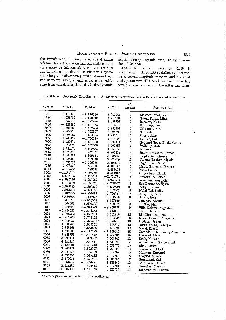
TABLE 4. Geocentric Coordinates of the Stations Determined in the Final Combination Solution

Station X, Mm I', Mmv ,

Z, Mm meters Station Name

102110347042703670ts770397040704570507075t u l o78r578167818790180158019900190029003900490059006900790089009901090119012' 90219023902590289029903190509065906690749077908090919113911491159177

1.118029- .521702

.M75r5- .828496- .1912862.3082392.46i,067

-r.2404791.130674

.6926281.3841744.5783704.6543375.426325

- r . , 1 ó ! ) / o /

4.5783284.579466

5.056125-3 .983776

5.105588-3 .946693

1.0182031.9427753.3768932.257829

.9762912.280589

- 5.466053- 1 .936782-3.977766-3 .910437

4.9037505.18&611 .6938031 .4897533 .9234114.3313103. 1839013.9074273 .9201784.595157

-2.45007L- 1 .264838

3.121280-6.007402

-4.876316-4.242049-5.177924-5.657458-4.967280-4.873597-5.534924-4.760229- 4 . 831368-4.347059-5.905685

.4579571 .959i34

- .229330- 5 . 166996

.457966

.586599- 5 . 166996

2.7L65773.743087

-.55õ2283.3662995.47L703

- 5.8040814.403576

-5.816919- 5 . 601398-4.9L4573-2.404282-5.077704

8.725L023.3763613.965201

- 3 . 653856-4.112328-4.467478

.299882

.Ðo/ÐrrL.42lM8I .602397

-.1347382.039425

-4.624421-3.466884

.592643- r . 111859

3.9429844.718731ó , ooo/ u/2.8168123.9832623 .3945801 .9855104.0489953 .9941114.6004831 .9665334.4037343 .8843663.3346Q83.4070424.4031794.3864083.401042

-2.775784-3.276566

3 .7696673.6988323.109623

- 1 .7969333. 1362501.3271602.880240

-3 .3554262.24217L3 .331916

-3.3030353.7292L7

.963872- .654325

-4.5566494.2873045.0029454.6330935.3227724.7638905 .0127083 .9126503 .6350355.1854675.572701

. 1.825730

1

F7

777

1010I,7

q

1055

1 D

5R

576

10I,7

uFl

5IÈl

o10Í2t215L4L2

Fl

1010Ià.f

t2t715

Blossom Point. Md.^ r ñ r i - .

Lirano .Ë orks. .Lvlrnn,Rosman, N. b.Edinburg Tex.Columbia, Mo.BermudaPuerto RicoDenver, Col.Goddard Space Flight CenterSudbury, Ont.JamaicaIlaute Provence, FranceStephanion, GreeceColomb-Bechar, AlgeriaOrgan Pass, N. M.IIaute Piovence, FranceNice, FranceOrgan Pass, N. M.Pretoria, S. AJricaWoomera, AustraliaSan Fernando, SpainTokvo. Japan¡Vaini hal. tn¿iaArequipa, PeruShiraz, IranCuraçao, A,ntillesJupiter, Fla.Villa Dolores, .A,rgentinaMaui, EawaüMt. Hopkìns, Ariz.Island Lagoon, ArætraliaDodaira, JapanAddis Ababa, EthiopiaNatal, BrazilComodoro Rivadavia, ArgentinaIlarvard, Mass.Delft, IlollandZimme¡wald, SwitzerlandRiga, LatviaUzghorod, USSRMalvern, EnglandDioysos, GreeceRosamund, Cal.Cold l¿ke, CanadaIlarestua, NorwayJohnston fsl., Paciûc

* Formal precision estimates of the coordinates.

4866

duced to absorb possible biases in either solu-tion that have the characteristic of a scale error.fn theory, this scale factor should be zero, sinceboth SAO and JPL have used the same valuefor GM, but 'pseudo' scale errors could be in-troduced. For example, a systematic error inthe refraction corrections to Baker-Nunn obser-vations could have an effect simiiar to a scaleertor.

In combining the JPL solution with the otherdata, the normalized covariance matrix suppliedby Mottinger was used. This matrix lyas scaledby his accuracy estimates for the components- of the station positions and preserves the strongcorrelation that exists between the lonEitudesof the soiution.

The results from the surface-gravity analysiscan be directly related to the combined solu-tion, since both refer to the same referenceellipsoid and GM. The zonal harmonics derivedby Kozai have not been i¡cluded in this com-bination, since his solution is quite independentof the satellite analysis of the tesseral har-úonics, and the surface-gravity data, becauseof their poor distribution, do not contain anysigniflcant zonal information.

The final combination solution contains atotal of 424 unknowns, 117 statipn coordinates,296 harmonic coeffcients, and 11 sca.ie, rotâtion,and translation parameters. In a solution ofthis kind, several iterations were made (as de-scribed above), ând several alternative weight-ing schemes were considered. These weightfactors are used to scale the covariance matricesderived fo¡ the individual solutions and in thecombination. As was already indicated, the co-variance mat¡ix of the geometric solution hasbeen multiplied by 2.8, and the covariancematrix of the surface-grayity results by 4.0,The covariance matrix of the dynamical solu-tion has been multiplied by 4.5 for the reasonsdescribed in the next section, whereas, for theJPL results, the accuracy estimates of Mot-tinger have been adopted without any furthermodification. This weighting scheme gives thebest agreement in the tests described in thenext section. The final results for station coordi-nates are presented in Table 4, and for har-monic coefficients in Table 5.

The power spectrum

G¡,poscrrxrx lNo Lerrsncr /TABLE 5. Fully Normalized Coefficients of thrSpherical Harmonic Expansion of the GeopotentiaiObtained in the Final Iteration of the Combination

Solution(C¿¡ arc the cosine terrns of degree I'and order z¿.

and S¡- are the sine terms.)

S¡-

2òùó

44À

5

6o6ô6o

77

7

77n7

8I888888IIIoIIooI

101010101 0101 01010101 1

2 2.4129E-061 1.9698E-062 8.92048473 6.86308-071 -5.2989E-072 3.30248-073 L89438-074 -7.96928-08I -5.38168-082 6.12868-073 -4 .30838-074 -2.66938{75 1.2593E-071 -9.8984E-082 5.48258-083 2.7873E-084 -4.0342F-r05 -2.11438-076 8.86938-08t 2.4L42E,472 2.8306E'473 2.0285E'474 -1.97278475 . -8.7024E'-106 -2.58478477 1.5916E-071 3.1254E-082 4.8r6rE-083 -5.74J48 084 -r.53788475 -5.67338{86 -5.39038{87 3.4390E-088 -7.73648-081 1.38238{72 6.67418-093 -9 .6463F-084 5.7125F485 -6.1435E{96 2.4186E-087 -5.0450F-O88 2.3359E{7I -8.24908-081 1.725tF-072 -3.1225E483 -2.33468484 -4.8185E-085 -8.00048-086 -3.2486E{87 5.4S61E{88 7.3957E{8I -6.8563F-09

10 7.2377î,071 4.3900E-09

-1.3641E462.60158-07

-6.3468E{71 .43048-06

-4.87658{77.06338{7

-7.5467F-073 .39288-07

-9.7905E48-3.5087E-07-8 .6663E-08

8 .30108-08-5 .9910E"O7

3.7652848-ó.Ðr/Õ11-u/

4.4626E-08-4.0388E{7-5.2264F-07-7.4756E-08

1 .15678-071.5645E-07

-2.34¿8847- 1 . 1390E-07

9.8461E-08i.0209E47

-6.7710E-082 .5696E-088.41408-081.80868{87 .5264E-086.16368-082.5930î-078 .9168E-086.76078-08

-1.6100F-08-8. i733E{8- I . 1817E-07

1.1183E-073.35518-092.2028847

-r.2700Fl75.72398{89.23268-08

-1.01678{7-i.0450E-07-1.41378-07-4.32488-08-r.4279847-2.01534E7

3.2003F.{8-7.9706E-08

6.2498F.O9-2.58858-08

2.9751E-08I

Ð (c,-2 / . t \C¡ : \ I . /nt )

' + s,^t)

EÅRr¡r's Gnav¡ry Frur,o eNn Sr¡trow CooRorx¿rns 4867

TABLE 5 (contùrud) TABLE 5 (contintted.\

Sl-8¿-C¿- Cu

1 11 11 11 l

1 1111 11 11 11 112L272L21 ,

12L21 9

12L212121 2

t ó

l ù

131313l Ð

T ó

13t ù

131313l41 À

L4t+741 ç1 A

T +

L4t4L4l 4 t

1 A

I J

l 5l .ð

I Ð

15I Ð

1515I A

15

2a

^

o,1

8o

101 1

I23A

678I

10I I

t2123A

É678o

101 1T2131,ö4

6,|

8I

1011T2131 À

12Õ4i)

617

8I

10

I Ð

1ô16161 616I O

1 6_tol o

161 6l o

I O

I O

16L O

17I I

t718181 ð

1 9191920202 l2 l,,

1 1t2f ð

15

2ó

K

6,7

8o

101 11 2t 2

1 Ã

-tÐ

I O

1213L4t2f ù

I412a ù

L4t 0

t413t4t4

4.8900E-08- ô . 3247E-08-3.01938-08

3.2523F-083 .7517E-084.57268"486.45468-081 .17508-07

-1 .1736E-071 .1785E-07

-4.5955F-082.74818-085.83868-08

-4 .3649E-082 .33758-08

-2.3868E-081.45078-08

-5.7854E-09-3.22328-08-1.8590E-08-4.49218-08- 1 .94078-08-5.60428{8-4.7456E48

2.3833E-08-1.99808-08

9.6637848-8.3417E-08-5.2217F'08-4.1759E-08-2.5623E,48

I .65898-08-3.3749848-1.32298-09-7.0288E-08-2.3090E-08

3.2120E-081.9042E{87.8017E-09

-2.5958E481.9140F,{81 .1061E-08

-3.0273F-084.9539E-085.3732E482.7833E-081.2481zu85 .15548-08

-5.2082E-08-3.5971F-09-4.4833E{8

8.3016E491.3916E-083.16848{87 .0020E-081 .18568{7

-9.76578{82.2064E-08

-2.0648E48

-9.1994H8-1.3r09E-07

5.4317F-08L.3215E 076.9005E49

-1.38628-07-1.6993E-08-9.94518-09-1.8900E-08-4.0688E-08-3. i0008-08

7.59868-085.47848-08

-2.22628-084.2637E'48

-6.6770E-109.97848-083.3752E-084.2858E-084.83828-09

-4.82068{8-5.7771848

2 .6288E-081.7367E{8

-2:89308-085.7030848

-4.7760E-085 .9782E-08

-3.2562E'49-2.0231E48

7.0767847- I .0528E-08

5.8541E488.2192E-087.4643E'484.9664E-08

-4.52898-081 .1919E49

-3.7527E,48-2.33448-08-5.8721848.8.41328{9

-6.08388{89.2345F"O8

-4.3168E-08;8.10378-08-5.7314F-08

4.5453848-1.28408-08

4.0142E-08-1.60568-08-5.7218E-09

6.6644E-081.82508-09

-r.r872F.474.2690848

-3.5710E482.66328{85.37248-10

-3.25858-081.05248-08

-3.7348E-081.2193E-081.4515F-09

-2.37898-082.1327E,48

-4.7358E-08-1 .1591F-08-4.4201F-08-5.8439E-08

1.0591E-07-8.4738E-08

9.00018-09-2.9849E-08

6.8502F-092.28348-083 .54758-08

-7.35908-09- 3 . 5485E-08-2.95228-08

8.3097E-083 .2749E-08

-1.6058E-081.1662E-084 .69038-09

-2.7M6E486.71158-083.3201848

- 3 . 9779E-095.83748{81 .11308-083 .6928E-095.2067E-08

-8.0549E-09

9.40528486.87268{94 .02498-09

-2 .6786E-08-1.4802E48

7 .6413E-083.0669E-083.26108-084 .30018-083.22308-08

-4.2809E-088.10088-09

-2.4677F'49-1.0628E-07-5.2467E,-10-7.07658-08- 3 . 4087E-08

2.0683E-08-2.2626E.08

8.4126E-i08.6217E-093 .5424E-094.2920F.102.72868{88.4724E,-09

- 3 .5547E-08-4.83768-08-8.26238-09-6.3'128E-08-2 .3817E-08

3.33208-08-1.6183848- 1 .6288E-08

3.0801E-102.6440848

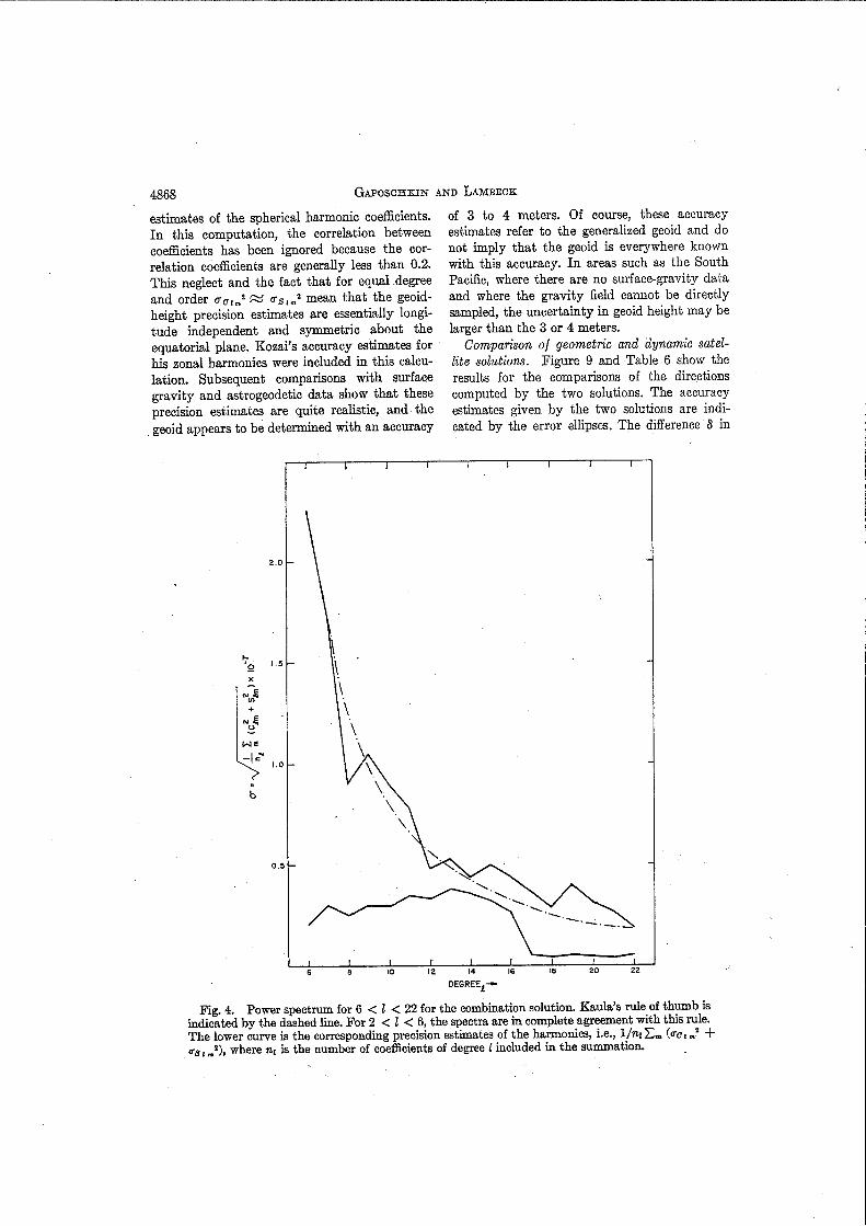
of the combination solution is given in Figure 4for I ) 6, where n¿ is the number of coefficientsof degree I included in the summation. They showa, remarkable adherence to the rule of thumba¡: tQ-s/lz.

Figure 5 gives the geoid corresponding to thenew' combination solution and a flattening ofI/298.258, Figure 6 shows the geoid couespond-ing to the hydrostatic flattening of 7/299.67,and Figure 7 is a plot of the free-air gravityanomalies corresponding to the combinâtionsoiution.

Table 4 contains the accuracy estimates of the'station coordinates. These estimates are the

formal statistics from the combination solution.but, as the subsequent compariÈons show, theyappear to be realistic.

Figure 8 illustrates the precision estimates ofthe geoid heights as computed from the precision

4868 G¡¡osc¡*rx ¿No L¿ìrsscr

estimates of the spherical harmonic coefrcients.In this computation, the correlation betweencoefficients has been ignored because the cor-relation coefficients are generally less than 0'2.This neglect and the fact that for equal degreeand order 6s¡^2 x, ds¡-2 mean that the geoid'

height precision estimates are essenti¿lly longi-

tude independent and symmetric about the

equatorial plane. Kozai's acculacy estimates forhis zonal harmonics were included in this calcu-lation. Subsequent comparisons with surfacegravity and astrogeodetic data show that theseprecision estimates are quite realistic, and the

geoid appears to be determined with an accuracy

of 3 to 4 meters. Of course, these acculacyestimates refer to the generalized geoitl and donot imply thaü the geoid is everywhere knownwith this accuracy. In areas such as tbe SouthPacific, where there are no surface-graviiy dataand where the gravity field cannot be direcilysampled, the uncertainty in geoid heiglrt may belarger than the 3 or 4 meters.

Compøríson ol geometri'c and dgno;rnic satel-lite solutions. Figure I and Table 6 show therezults for the comparisons of the directionscomputed by the two solutions. The accuracyestimates given by the two solutions are indi-cated by the error ellipses. The difference I in

, o

x

N i

+N ì

t 4

oEGREET+

Fig. 4. Power spectrum ior 6 < t < 22 for the combination solution. K¿ula's rule of thumb is

i"¿i.ä.¿ by tle dashed line. For 2 < t < 6, the spectra are in complete.agreement with tbis rule.

The lower curve is the corresponding precision estimates of the harmonics, i.e., L/n¡f^ (as ¡ *? *

øs ¡ _r), where z¡ is the number of coèfficients of degree I included in the summation.

trlaRru's GRavrry Fr¡¡,o ¿xp Sr¿rro¡r Coonolt¡¿'tus

Fig. 5. Geoid heights in meters of the new combination solution corresponding to areference ellipsoid of flaùtening Í - 7/298258. (Contour interval is 10 meters, and shadedareas are regions of negative geoid heighü.)

the positions derived from the individual solu-tions is a good i¡dication of the ¿ccuracies thatcan be expected for the combination-solutioncoordinates, although it must be pointed outthat in Figure 9 the difference between the twosolutions results from uncerta.inties in the co-ordinãtes of both stations and that at each

station a, numbbr of such comparisons ca:rusually be made. Thus, the accuracy of thestation positions relative to the origin of thecoordinate system should be better than theseûgures indicate.

The accuracy estimates oc of the geometricsolution directions are obtained by the method

+90.

+80.

+60'

+40.

+2O"

o.

-?e

-40.

-60.

-80.

-90.-l8O' -160" -l4O' -120" -lOO' -80" '0"

+ZO" +4Oo +60. +gO. itOO. +tZO" +t40. +t6O" +tg6.

Fig. 6. Geoid heights, in meüers of the new combination solution corresponrling to a¡eference ellipsoid sf fl¿lþning | - L/255.67. (Contour int¿rval is 10 meters, and shadedar€as are regions of negative geoid height.)

-l8O' -160" -l4O' -120" -lOO9 -8Oo O. +20. +4O" +600 +eO" +tOO. +t20" +t40" +t6O" +tgg"

G¡poscgr¡r.I ¡Np Leltnncr

Fig. 7. Free-air gravity anomalies with respect to the best fitting ellipsoid' I - l/298258

from" the adopted ãolutión (lO-mgal contours; darker shaded areas åre regions of negativeanomalies).

described earlier. The dynamic solution, how-ever, gives accúracy estimates for the coordi-nates, and consequently for the station-stationvectors a¡, thaí are. overop.timistic: This isusually evident from figures such as Figure 9,where 8" is often considerably greater thaneither o¡',or on'. Making an analysis similar tothat used i:r the geometric solution Jor estab-lishing the accuracy indicates that the covari-ance matúx of the dynamic solution should bemultiplied by a factor of ËJ - 4.5. Whenharmonic coefficients derived from differentiterations of the dynamic satellite solution arecompared, it also appeârs that the formalvaria¡ces must be multiplied. by a factor ofabout 5 in order to obtain realistic accuracyestimates.

Figure 9 also indicates the directions of thestation-station vector derived from the combi-nation solution compared with the geometlicand dynamic results. In view of the above, thesecomparisons indicate that for the funda,mentalBaker-Nunn stations (those numbered 9001 to9012) the combination-solution coordinatesshould be reliable to better than 10 meters.For the new Baker-Nunn staùions (9021, 9028,9029, 9031, and 9091), from which there arefewer observations, the comparisons indicatethat the combination-solution coordinates should

be reliable to better than 15 meters. These estimates are in agreement with the formal statistic.given in Table 4. The longitude di.fference between the trvo satellite solutions obtained fronthe combination solution is -0.2 t 0'5 ¡tracrand is not significant,.. Compørisan uith søteLlite orbi'ts. Each soiu

! 9 0

t¡J

t--t-j

+ a ^

t 6 0

0 l .o 2 .o 3 .o 4 .øø,. (m)

Fig. 8. Precision estimates of geoid heightsdetermined from the harmonic coefrcient pre-cision estimates.

H E I G H T

l O m/ \^, /\ - r '

\ o.urr"

9029 - 90315257 tm \(,

- )r'

-Fig. g. Comparisons for station+tation vectors computed from (triangle) the geometric

solution, (sQuare) the dynamic solútion, and (diamond) the combination*solution.-The twoerror ellipses centered at the squaie refer to the formal statistics of úhe dynamic soluüion(the inner ellipse) and after the covaúance matúx has been multiplied Uy the f.actor k"(outer ellipse).

4871

sibly 5 meters), and unmodeled periodic per-turbations.

Comparison of søtellite and deep-spone-probesolutior¿s. In order to compare the satellite andJPL soiutions, a combination solution usinsonly the satellite and surface-gra.üty informa-tion has been made. Table 7 gives the resultsfor those Baker-Nunn stations that are relateclto ihe JPL antennas. From the ground-surveyinformation given by Gaposchkin ond Lambeclc[1970, Table 10], the coordinates for the JpLsites in ihe SAO system can be computed, andthe differences in longitude AÀ¡ and in distance

Elnrs's Gn¿v¡ry Frnr¡ ¿No Srarro¡r Coon¡r¡¡¿rrs

tion resulted in improved orbitai residuals; forthe final solution, the orbital residuals for éatel-lites such as Geos 1 or Geos 2 are less than10 meters. These orbits are computed from acombination of laser and Baker-Nunn data fo¡30 days. The rms residuals for the optical dataare 2 arcsec. The laser data have an accuracyof 1 to 2 meters. The rms is 7 meters in allcases, and no residuals exceed 10 meters. Theseare orbits with significant amounts of laser datafrom 2 or 3 stations. The 7-meter orbital errorscan arise from stabion-coordinate errors (prob-ably about 5 meters), geopotential errors (pos-

H E I G H I

Jt:,l O ñ

/'

/ / - - - .' ( . )\ r '\ / '

A Z I M U T H

,/t A

9007 - 90r I| 826 hn

487.2 G¿posc¡rrr¡¡ ¿wo Lentsncrto the rotation axis Ar, are given in Table g.This tabie aiso gives the ac-curac5, .rti_itu.from the statistics provided n1, tlå tw;;Ì"_iions and the ground survey. The differences inlongitude ìmmediatell reiect the .y.t._rtì,rongl[ucte dlfterences between the trvo solutions:the JPL longitudes are to the east of t¡. SÁOlongitudes. From the over_all combination solu_

. tion, these transformation parameters ,r, *ll.Ofor and yield (aÀ) = _8.2 =t O.S ¡rraã- anaar/r - (+0.¡ * 0.5) 10-. the scale of theSAO system as defined by the station .*.d,nates being larger than that of the JpL.V.i.*

The residuais (AÀ) - AÀ¿ and (Ar¡ _ 6r,are in ali cases iess than 10 meters and supportthe accuracy estimates given in tubju i'io,stations 9002, 9008, g004, and g1t3. Table Sgìves the adjusted coordinates of the Jplìta_tions in ihe SAO reference sysrem.

The longitude difference cannot be attributedto the difference in the UT1 time .y.t.*. ur"áþI ú. two agencies, since at the iime .f-rfr.Mariner 5 observations, UT1 (JpL) _ UTC =89.0 msec and UTI(SAO) _ UTC _ lõr.+msec, so that the expected longitude difference

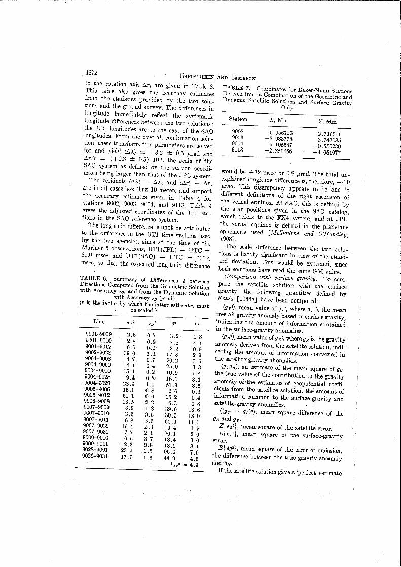
TSBTF 6. Summary of Differences ô betweenDirecúions Computed-from the Geomãi.; $I";ii";wrth ¡{ccuracy o6, â,nd from the Dynamic S;i;ü;;- wiih Accuracy

"o çprad¡(È is the factor by *hich tieÍaìiåii'"timutes mustbe scaied.)

II.BLT: Coo^rdinates for Baker-Nunn Srarionsue¡rved from a Combination of th. G;;";ri";;îDynamic Satellite Soluti,O,ltT ""d

Surface Graviry

Station X, Mm It, Mm

9002900390049113

5.0õ6126-3 .983778

õ.105587-2 .350466

2.7L65r13.743085

- 0 . 555230-4.651977

Line ac2 k2o 'oD2

wou.ld be *12 msec or 0.g ¡.rrad. The total un_explained longitude di_fference is, therefore, _4.0p¡ad. This discrepancy âppears to be due todrterent defi¡itions of the riglit ascension ofthe vernal eq¡.rinox. At SAO, tU, i. auÀo.J Uïthe. star

-positions given in ihe SAO catalos,u/n¡cn refers to the FK4 system, ancl at ,Ipi,the vernal equinox is definãd in the planetaryephemeris used lMelbotìrne únd O;Hd;ctl;a,ie68l .

The scale difference between the two solu_tions js hardly significant in view of t¡. ,troO_ard deviatjon. This would be expected, sìnceboth solutions have used the same

^Cif¿ ,ä"..

Cornparíson with surføce grauitg. fo .o*_pare the satellite solution with the surfacegavjtf, the following quantities defined byKaula llg66al have been computed:

(g7r), mean value of grr, wheìegz is the meanfree-air. gravìty anomaly ba.ud oo .u.fu.. ;;r;rrr,rndrcatrng the amount of information containedin úhe.surface-gravity anomalies.

(gg2), mcan value of gsr, where gs is the gravityanomaly derjved from the satellite solut;oã, indi_cating the amount of information contai¡ea lothe satellite.gravity anomalies.

\grgt), an estimate of the mean square of g¿,the true value of the contribution to ìhe gr*rriöanomaly of,the estímates of geopotential-coeff_cients from the.satellite solutionj tn.

"-ou:ri of

information cortrmotr to the surfac*g.ruitiu"ãsatellite-grav,ity anomalies.

9001-90099001-90109001-90129002-90289004-90089004-90099004-90109004-90289004-90299005-9006eoqs-gO129006-90089007-90099007-90109007-90119007-90299007-90319009-90109009-90119028-90919029-9031

2 . 6 0 . 72 . 8 0 . 96 .5 0 , . 2

3 9 . 0 1 . 34 . 7 0 . 7

74.r 0 .41 5 . 1 0 . 29 . 4 0 . 8 .

28 .9 1 .01 6 . 1 0 . 86 1 . 1 0 . 61 3 . 5 2 . 23 . 9 1 . 82 . 6 0 . 56 . 8 3 . 6

1 6 . 4 2 . 3t 7 . 7 2 . t6 . 5 3 . 72 . 3 0 . 8

2 3 . 9 . 1 . 51 n -L t . t I . o

3 . 2 1 . 87 . 8 4 . r3 . 2 0 . 9

57 .8 2 .920.2 7 .525 .0 3 .31 0 . 9 L . 41 6 . 0 3 . 15 1 . 9 3 . 52 . 6 o . B

r5 .2 0 .46 . 3 0 . 8

3 9 . 6 1 3 . 63 0 . 2 1 8 . 96 0 . 9 t r . 71 4 . 4 1 . 520 .L 2 .0r 8 . 4 3 . 61 3 . 0 8 . 19 6 . 0 7 , 64 4 . 9 4 . 6

& " o s : 4 . 9

((s, - gg)z), mean square difference of thegs and g,1.

E_lrtr!; mean square of the satellite error.Í;lerzt, mean bquare of the surface-gravity

etror.

.,81..!!, l ,mean squarè of the er¡or of omissicjn,the difrerence between the true gravity

"no*"fyd,nd ga.' If thesatellite solution gave a ,perfect, estimete

E¿nmr's Gn¿vrrv Fr¡r,¡ ¡xo Sr¡rroN Coon¡rN¿tps 4873

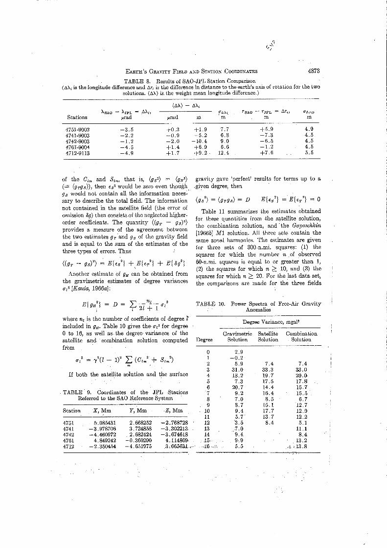
TABLE 8. Results of SAO-JPL Station Comparison(aÀ¡ is the longitude difference and Ar, is the difference i¡ distancê to the earth's axis of rotation for the two

solutions. (ax) is the weight mean longitude difference')

(ax) - ^Àr

Stationst r s , r o - À ¡ p r , : { t r ; t

prad ¡rfadljlim

fS¡O - T¡p¡, : AT,, úArt ,

m m

475L-90024741-90034742-9003476I-900447r2-9tr3

- 3 . 5- 2 . 2

- 4 . - o- 4 . 9

t Ð . v- 7 . 3- 6 . 5

f / . o

4 . 9+ - Ð4 . 54 . 55 . 5

+ 0 . 3 + 1 . 9 7 . 7- 0 . 9 - 5 . 2 6 . 8- 2 . 0 - 1 0 . 4 9 . 0+ 1 . 4 + 6 . 9 6 . 6+ t .7 +9 .2 - 12 .4

of the Cn and S¿-, that is, (g"') : (g"\(= (Stg")), then es2 would be zero even thoughgs would not contain ail the information neces-sary to describe the total fietd. The informâtionnot contai¡ed in the saùellite fielcl (the error ofomission ôg) then consists of the neglected hiþher-order coefficients. The quantity ((5, - Sù')provides å measure of the agreement betweenthe two estimâtes gr'and gs of the gravity fieldand is equal to the sum of the estimates of thethree types of errors. Thus i

( (s , - s" ) ' ) : E{r r ' ] t l ,E ler ' l * E lõs" j

Another estimate o1 g¡¡ can be obtained fromthe gravimetric estimates of degree varianceso¿2 fKøula, 1966ø] :

øts f t : D : Ðn?¡ , :where rc¿ is the number of coefficients of degree linciuded in g¡¡. Table 10 gives the ø¿2 for degree0 to 16, as well as the degree v¿riances of thesatellite and combination solution computedfrom

o , ' : 7 ' ( l - Ð ' t ( C , ^ ' * S , * " )

If both the sateìlite solution and the surface

TABLE 9. Coordinates of the JPL SiationsReferred to the SA,O Reference System

Station X, Mm I., Mm Z, Mm

gravity gave 'perfect' results for terms up to agiven degree, then

( ø " 1 : k r s " ) : n ¿ ' { é " ' } : E l e r 2 l : 0

Table 11 summarizes the estimates obtainedfor these quantities from dhe satellite solution,the combination solution, and the Gaposchlcin

[1966ö] M1 solution. ÀlI three sets contain thesame zonal harmonics. The estimates are givenfor three sels of 300-n.mi. squares: (1) thesquares for which the number n of observed60-n.mi. squares is equal to or greater than 1,(2) the squares for which z ) 10, and (3) thesquares for which n ) 20. For the last data set,the comparisons are mâde for the three fields

TABLE 10. Power Spectra of Free-Ajr GravityAnomalies

Degree Variance, mgalz

DegreeGravimetric

SolutionSatellite CombinationSolution . Solution

+ I Ð L

47474742476L47L2

5.085451 2.668252-3.978706 3.724858-4.460972 2.682424

4.849242 -0.360290-2.3504:rr4 -4.651975

-2.768728-3.302213,-3.674618

4.114869,ó . O O Ð O ó 1 . , ' ì

012óÀ.56,7

8I

. 1 0I I1 2l3t4

, ,15 ' ,, , , 1 6 , , t :

2 . 9-0 .2

5 . 93 1 . 018.2

t . ¿

20.79 . 27 . 08 . 79 . 4' 3 . 5

7 . 09 . 49 . 9a . 5

a À

3 3 . 3r9.717 .514.416 .48 . 5

15 . 117 .713.78 . 4

33 .020 .017 .81 È a

l D . j )

D . /'12.7

72.912.2

1 1 . 18 . 4

13.2, i i 1 3 . 8

4874

TABLE 11.. Geposcr{KlN ¿rrro L.lrrspcx

Comparison of Søtellite ,"d Co-?#jil¡ Sot"tio* with Surface.Gravity Measurements

Solution (9, - gs) ') Qrss) ks') D kr ' ) E le¿21 E le7z l E íôS ' l

Combi¡r¿tion solutionSatellite solutionMl solution

Combination solutionSatellite solutionMl solution

Combination solutionS 8 , z ¡ ¿ ( 8( 10 ,22 1 10( 1 l , r n l 1 1

! 1 2 , m 1 1 2! L 4 , m 1 1 4( 1 6 , r ¿ 1 1 6

Satellite solution( 8 , z ¿ 3 8( 10,22 ( 10! L l , m ! L l! 1 2 , m ! t 2! L 4 , m 1 L 4

Total ûeld

Ml solution1 1 8 , m 3 8Total"ûeld

n ) 7, N : 936, 300q,.mi. squares206 146 225 163 274272 110 218 143 274242 90 148 108 274

n ) 70, N : 369, 300m.m,i. squares135 195 230 163 297250 127 2t2 L43 297222 r02 131 108 297

n ) 20, N : 136, 300-n.mi. squ(ffes

70

10858

358529

15212311611387пt

L02120126129146163

165 90r32 119135 126134 Lzg109 15675 184

727272

191919

oo9279

83151176

ot1 1 6r34138166186

98110126128IÐU

161

85101

253 2253 -3253 8253 I253 10253

253 L2zi)B I253 ll253 17253 33253 43

253 0253 7

1111t l1 11 11 1

L79L45151163L l ó

177

86109115111LT7118

102120126t29146143

11 15611 13311 12711 13111 12511 t24

1 l1 1

t02108

\ 168 85168 93

t57148

x5. AREA MEANS- coMBINATtON SOLUT¡ON

LONG¡TUDE.

Fig. 10a. North Atlautic. 4

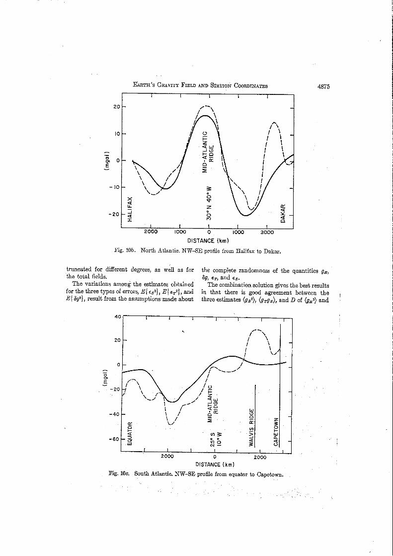
Fig. 10. Comparisons of continuous gravity proûlespiled by Talwani and Le Pichon (broken lines) withtion solution (solid lines).

- +32.5'.

from shipboard measurements com'proûles computed from the combina-

-20

trrurcated for diferent degrees, as wéI as forthe toüal fields.

The variations amonpj the estimates obtainedfor the three types of errors, E{rrrl, E{eyll, andE | 6grl , resulú from the assumptions made about

4875

the complete randomness of the quantities g¡.,ð9, e7, and es.

The combination solution gives the best resultsin that there is good agreement between thethree estimates (gsr), (grg"), and D of (g"z) and

E¿nrrr's Gn¿v¡rx F¡¡r,o ¿No Sr¿rroñ Coonor¡r¿rss

20

t ^

ct! v

2000 tooo 2000DISTANCE (km)

Fig. 10b. North -A.tlantie. NWÆE proflle from llalifax to Dakar.

4 0

oÈ

o

- 4 0

- o u

2000 o 2OOODISTANCE (km)

Fig. 10c. South Atlantic. NW-SE proÊle from equator to Capetown.

Fz.< r J

ô

=oolr

z.oolo

\, \

/ ìII,

X

lrJ

-

\\

I

//

I

II!

tIIIII

I¡l I

P Iocl

IØ l; lJ I

Ét

\\

z=oFl¡l.L

C)

,/í-__

/ . / r ¡f =/ 2

u ' - jUã 9

t eô -=

ø jo o| r ) oô t -

tt-r'

l -t\\

o

lo¡¡¡

5o x So AVERAGESCOMBINATION SOLUTION

,'/

Z ^ \

U

=

\

c

-20

- 4 0

- o u

60c goc

LONGITUDE

Fig. 10d. fndian Ocea¡. d = 0..

the E{esz} and ((gu - gr),) are small. Theuegative value Tor Elrurl when Z : 10 is causedby the combi¡ation solqtion containing thegravity anomalies agaiast which the tests aremade. The estimates of the errors of omission

are still quite large when compared with theestimates of e¡2 and e12, indicating that thesurface-gravily data have additional i¡Jorma-tion that has not been extracted. in this solution.

These tests, however, are not entirely valid

l o

ÞoE

80" lOO"LONGITUDE

Fig. 10ø. I¡dian Ocea¡. ç = -26..

i lt lt lt l

t l' o lz lo lz l< l

.z o lz l- l

a lo lz lo l- l

6 lz lr lr l

ItI

(n=t¡lt-U)g)

t¡l(9

c9t-zJF

_- - 5Ox 50 AVERAGES_ COMBINATION SOLUTION

l¡JJF-z

I¡Jl¡¡frlÀ

Øt-

=I

r\-.-

ì..-__r'- t/__-

t ?oc

E¿nrs's Gn¿y¡rr Fnr,o ¿rro Sr¡.rro¡r Coon¡rN¿rus 4877TABI;E 12. Summary of Comparisons between Su¡fae+.Gravity Measurements g7 by Talwani and Iæ

Pichon and Gravity Anomalies gs Computed from the Combination Solution for Selected Profiles

Profile(@s - sr)'),

mgal2

- 2

Å&i, 6cB2: <(gs - 9.7) ' ) - asr2,mgâr"

ó : 32.5" North AtlanticNW-SE North AtlanticNW-SE South Atlanticó : 0o Indian Oceanó : -25" Indian Ocean

8468

22280

166

2525252525

5943

t97Ða

1 À À

for the combination solution, since the gE, ôg,ea, and €s a,rê Do longer independent. A betterestimate of ,E{ es,} can be obtained from lhe os,øs of the combiaation solution as indicated byLatnbeclc [1971ö]. For the total freld Eleszl : 34mgalz, giving ElAgz¡ : 30 mgal2. AIso, theestimate oL EleT,l is likely to be too small, sof,hat Elðgz) is even further reduced, and irreality there does not seem to be very muchadditional i¡formation in the surface-gravitydata used. i

The results obtained from the satellite solu-tjon alone are not in such,,good agreement withthe surface-gravity data as is the combinationsolution. For a gravity field complete to 8, 8,lhe Ml and the new satellite solution give almost

(oo "')

= 99 mgal2 = 10 m2

equivalent comparisons. For both, the E{ esr}are small and there is good agreement among(grgul, (ggz], and D, indicatiag that the twosolutions are equivalent and that they containmost of the information in a tcorrect' 8, 8 field.At 10, 10, the new satellite solution showsa marked improvement in the comparison((g, - gs)r), and this field also appears tÒ beas good as can be expected. But beyond aboutthe 11th order, the comparisons deteriorateand the E{.ur} increase.

Further tests with surface-gravity data weremade by use of the recent compiiations by ?al-wani and, LePi.chon 119691 for the AtlanticOcea¡ and for the fndian Oeean lLe Pi,chon andTalwtn|1969l. Figure 10 shows free-air grav-

- t - - t t t t t t t z l - -

\ \ \ \ \

\ \

260.LATITUOE

F ig . Uø . ç :35 ' .

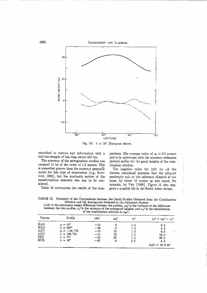
FiS. 11. Comparisons between geoid proûles obtained from the combination golution(solid lines) and profiles obtained from asürogeodetic measure-ua1g f,¡qnsformed into theglobal reference system (dashed lines). The difierence between the üwo proûles, after thesystematic part has been subtrå.€ted, is shown by the dot-da"sh lines.

t-

oU

o

U

ity-anomaly profiles computed from 5o X 5oarea mear$ from these compilations and fromthe combi¡ation solution. With The exceptionof the first, these profiles are taken along theships' tracks where contínuous gravity measure-ments we¡e obtained. The first, profile, alonglatitude 32.5' in the North Atlantic, is midwaybetw-een two parallel ship cruises. All profilesare teferenced to the international gravity for-muia. The âccuracy of the 5o X 5o area meansis assumed to be 5 mgal.

Table 12 gives ((gg - go)") for each of theseprofiles, and from these numbers the accuracyof the gravity anomalies computed from thecombination solution can be. computed. Theaverage yalue is 10 mgal, .or about 3.5 metersin geoid height. This average accuracy estim¿tr.is in good agreement wiih the previous esti-mates.

Compørison wi,th astrogeod,eti,c d.atø. Geoidheights obtained from astrogeodetic leveling areavailable for several major datums. These data,Iike the zurfaee-gravity dala, could be used asa further input in the combination solution.Elowever, the coverage extends only to areaswhere reliable surface-gravity.data are alsoavailable, and the contribution of the additionalinformationrto the global solution is not very

G¿roscsrrm ¿wn L¿lrspcr

LATITUOE

Fig. 11b. À - 260'. North American d¿tum.

- ?o

significant. fnstead, the astrogeodetic data havebeen used for comparison, thus providiag anindependent estimate of the accuracy of theglobal solution.

To compare astrogeodetic geoid proûies with

- l o

EØF - 2 0

(9l¡J-g -30

l¡l(9

- 4 0

E 2 ãÌ-9U

o( 9 O

- t o

LAT I TUOE

Fig. l1a I=136.25 ' .

j

4879

tsIU¿ ooo

0- l o

l l 6 "

the giobal solution,' it is necessary that theformer refer to an ellipsoid, with its origin atthe earth's mass center and of the same dimen-sions and parallel to the'ellipsoid of referenceused for the global solution. The transforma-tion elements are given for severaL major datumsby Lømbeclc l7971al. When these transforma-tions cont¿in rotation elements, at ieast part ofthe systematic errors in the astrogeodetic heightsis absorbed. In the case of the Indian datum,only one station is available for establishing thereiationship between the datum and the globalsolution. Thus only the three translation êle-ments could be determi¡ed, and a systematictilt can be expected.

The following proflles were compared:

1. The geoid section along the 34th parallelin North America given by Rice 11962l.

2. A section along the meridian of 260o from65"N to 18oN, selected from X¡s sempilationby Fischer et ol. 11967l for the North Ameri-can datum (NAD).

3. Two profrles across Australia, óne alongthe latitude circie of -30o and the other alongthe meridian of 138o, given by Fischer and,Slutshs [1969].

4. A proûle along the meridian of 75othrough Indta lSuruey of Ind,i,ø,79571.

. l zo" l z4" t?a" t32 . t36 . t40" t44" l+e .LATITUOE

Fig. 11d. ç - -28.75'. Austr¿lian Geodetic datum.

5. A profile along the meridian of 16"through central Europe lFischer, 19671.

Figure Ll gives the results. All profiles referto a reference ellipsoid with ø'= 6378L55 metersa¡nd 1,/l = 298.25. The astrogeodetic profiles are

l O m

oU

a - -////

30. to"LATITUDE

tr'ig. 11e. À = 75o. India¡r datum.

- 120

E¿nrg's Gn¿v¡rr Fr¡r,o ¿wn Sr¿r¡ox CoonorNATDs

,/

-\\- \ s * _ _ _ - - _ _

,/ ,// .--f'"-------rr. t t t / ' '

-1--'.'-< /'/i

./'- . - ' ' ' / '

./a"

E'F

1

UJI

õU

G¿posc¡lrr¡¡ ¿¡ro Le¡¡sncr

\ - / - \\ \ \ -?¿',^==.------_<í- \------\ - . - . - /

\\ \ . \

- \

LATITUOE-

Fie. lU. ì, = 16', European datum.

smoothed to remove any information with ahalf-wavelength of less than about 200 lm'.

The accuracy of the astrogeodetic profiles wasâssumed 'to be of the order of 1.5 meters. Thisis somewhat greater than the accuracy generaüjtstated for this type of observation le.g., Bom-ford., L9621, but the stochastic nature of thetransformation elements also has to be con-sidered.

.Table 13 summarizes the resr:lts of the com-

parisons. The average value of os is 3.2 metersand is i¡ agreement with the acuJtàcy estimatesderived earlier for the geoid heighis of the com-bination solution.

The negative vaiue for (Ai.) for all thedatums considered ildicates that the adoptedsemimajor axis of the reference ellipsoid is toolarge, by about 15 meters

", *", noted, for

s¡ample, by Vei,s [1968]. Figure 11 also sug-gests a possible tilt in the South Asian datum.

TABUE 13. Summary of the Comparisons between the Geoid Profiles Obtained from the CombinationSolution a1d the Astrogeoids Referred to the Geocentric System

((Al¿) is the systematic height difference between the proûles, ø6¡2 is the oriaoc" of the differencebetween the two proflles, co! is the variance of the astrogeoiá héightß, and asz is the contribution

, of the combi¡s,tion solution to ø¡¡2.)

Datum Profrle (A¡¿) c.i¡z dov øs2: o6hz - oo l

NADNÄDAGDAGDINDEUR

- 1 5- 1 6-12-L2-36-42

1 . 5r . o

l . a

1 . 5

d : 3 5 otr : 260öö : - 28 . ' 75I : 136."25À : 7 5 'À : 1 6 o

86

10t2306

o . ô4 . 58 . 5

10 .528.5

f t . a)

(os') : 10.5 mt

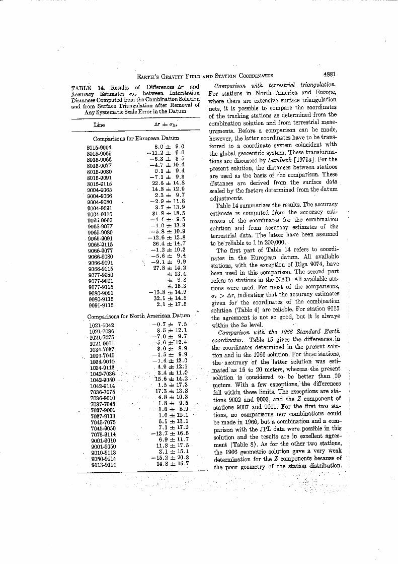
TABI;E L4. Results of Difierences Ar and

Accuraey Estimates ø6' b9twe99 InterstationDistances Computed from the Combination Solutionand from Surface Triangulation after Removal of

Any Systematic Scale Error in the Datum

Eents's Gnev¡rv Fmr¡ exo Sretro¡¡ Coonorx¿rss 4881

Compørison witlr terrestrial trì'angulati'on'

For stations in North America and Europe,

where there are extensive surface triangulationnets, it is possible to compare the coordi¡ates

of the tracking stations as determined from the

combination solution and from terrestrial meas-

urements. Before a compadson can be made,

however, the Iatter coordinates have to be trans-

ferred to a coordinate system coincident with

the gtobal geocentric system. These transforma-

tions are discussed by Lom,beclc 1L971'ø1. For the

present solution, the distances between stations

ãre used as the basis of the colaparison' These

distances are derived from the surface data

scaled by the factors determined from the datum

adjustments.Table 14 summaïizes the resuits. The accuracy

estimate is computed fiom the accuracy esti-

mates of the coordinates for the combination

solution and. from accuracy estimates of the

terrestrial data. The latter have been assumed

to be reiiable to 1 in 200,000.The first part of Table 14 refers to coordi-

nates in the European datum. Ail available

stations, with the exception of Riga 9074, have

been used in this comparison. The second pari

refers to stations in the NAD' All available sta-

tions were used. For most of the comparisons,

o, ) ùr, indicating that the accuracy estimates

given for' the coordi¡ates of the combina-tion

*lotioo (Table 4) are reüable. For station 9115

the agreement is not so good, but it is always

within the 3o level.Compartson wí'th the 1966 Stondørd' Earth

coord,i,nates. Table 15 gives the difrerences in

the coordinates determined in the present solu-

tion and in the 1966 solution. For these stations,

the accuracy of the latter solution was esti'

mated as 15 to 20 meters, wherea's the presènt

solùtion is considered to be better than 10

meters. Tfith a few exceptions,-the differences

fall within these lìmits. The exceptions are sta-

tions 9002 and 9003, and the Z component of

stations 9007 a¡d 9011. For the first two sta'

tions, no comparisons nor combi¡ations could

be made in 1966, but a combination and a com-

parison with the JPL data were possible in this

solution and the results are in excellent agree-

ment (Table 8). As for the other two statio.ns,

the 1966 geometric solution gave a, very weak

determination for the Z components bæause of

the poor geometry of the station distribution'

tine Ar + .6L t

Compãrisons for EuroPean Datum

801F90048015-90658015-90668015-90778015-90808015-90918015-9115900490659004-906690049080900+90919004-91159065-90669065-90779065-90809065-90919065-9115906G90779066-90809066-90919066-91159077-90809077-90919077-91159080-90919080-91159091-9115

8 . 0 + 9 . 0- 1 1 . 2 + 9 . 6- 6 . 3 + 3 . 5-4.7 * L0 -4

0 .1 : t 9 .4- 7 . 1 L 9 . 322.6 + 14.814 .8 + 12 .92 . 3 + 9 . 7

- 2 . 9 + 1 1 . 83 . 7 + 1 3 . 9

3 1 . 8 + 1 8 . 5-4 .4 + . 9 .5- 1 . 0 + 1 3 . 9- 5 . 8 + 1 0 . 9

-12 .6 * 13 .836.4 + 14.7

- 1 . 2 + 1 0 . 3- 5 . 6 + 9 . 4

. , - 9 . 1 + 9 . 9' 27.8 + L4.2

+ 13 .4+ 9 . 8+ 15 .3

- 1 5 . 8 + 1 4 . 932.L +.14.52 .L + L7 .5

CorÍparisons for North American Datum

L02t-L0421021-7036102L:70751021-90011ße7037L034-704510349010103,L9113L042-7036104%s050t042-grl+703ï707570e&90107037:10457037-90017037-9113704 075704F90507075-9LL49001-90109001-90509010-91139050-91149113-9114

-0 .7 + 7 .53 . 5 + 1 2 . 1

-7 .0 +. 9.7-5 .6 {12 .4

3 . 0 + 8 . 9- 1 . 5 + 9 . 9: 1 . 4 + 1 3 . 0

4.9 + Lz. t3 .4 + 11 .0'15.6 + 14.2 .1 .5 + 17 .3

17 .3_+ 13 .84 .8 + 10 .31 . 8 + 9 . 5

. 1 . 6 + 8 . 91 . 6 + 1 2 . 16 . 1 + 1 3 . 17 . t * , L7 .2

-13 .7 ' : t 16 .56 . 9 + 1 1 . 7

1 1 . 8 : t 1 7 . 53 . 1 + 1 5 . 1

- !5 .2 + .20 .314:8 +15.7

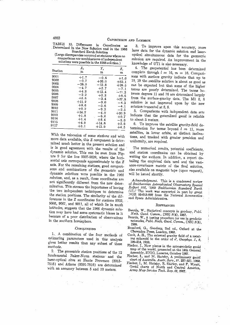
4882 G¿poscgr¡¡r ¡,rqo Le¡¿¡pcr

solutions were possible i.ttãróiri ."1äì"îî

X, Y,ùtaflon m

IABtq 15.' Di_ffe¡ences in Coordinates asIJerermmed rn the New Solution and i¿ the lg66Standard Earth Solution

(Large discrepancies occur¡ed atsiàäons wlere nocor_nparisons nor combinations of inaepenãenf-

- 3. To improve upon this accuracy, morelaser data for the dynamic solution ,oá lr""r_optical simultaneous data for tn" g."*ri¡.solution are required. An improvem"it io tiruhowledge of UTl is also necessary.

4. The geopotential has been determinedcomplete through I ,-, 16, rn = 16. Comoari_yns ø!h surface gravity indicate that up to10, 10 the satellite solution is about as sooi ascan be expected but that some of the hisherterms are poorly determined. The terms be-tween degrees 11 and 16 are determined. largelyf¡om. the surface-gravity data. The Ml g", gsolution is not improved upon by the íewsolution tn:¡cated at 8, 8.

5. Comparisoas with independent data. setsindicate that the generaüzed geoid is reliableto about 3 meters.

6. To improve the satellite gravity_fieid de_termination for terms beyond J ,=. 11; moresatellites, i¡ lower orbits, at distinct inclina_tions, and tracked with greater precision anduniformity, are required.

The numerical results, potential coeffcients.and station coordinates can be obtained bvwriting the authors. In ad.dition, a report de_tailing the empirical data used. and tle vari_ance-covariance matrlx of the final solution.also available on magnetic tape (upon request),will be issued shortly.

-Aclannwled4ment. This is a condensed reviewof. Smithsonian Astrophysícal Obseruatori A"i¿"1H_eþort 315, ,1969 Smithsonian Standøid

'Earth

!!2i T\. work was zupporied in part ¡y s""iNGR 094154û2 from tlie Naiional ¡.";o"Tti;;

.and Space Administration.

R¡reno¡rcnsBaarda, W., Statistical eoncepts in geodesy, pzö1.^Neth. Geod,. Cotnm, INSI'Z(4), i%1.--'

- -""'

.Éaãr.d.a., JY" { le¡iing procedure for use in seodeticneüworks, PubI. Neth. Geod,. Comtn., t¡VSl ãiãj,1968.

Bomford,, G., Geodesy, 2nd ed., Oxford at the_ urarendon t ress, J,ond.on, 1962.Cook, A- I[.,.The extemal $avity ûeld of a rotat_

ing spheroid to the ordei of "",

O"oeigr.- t.lz,199-214, 1959.

z,m

90019002900390049005900690079008900990i0901 I9012911491 159117

- u . t- 2 6 . 0- 4 . 7

+4.3- 2 . 2-1-Ð.o

-t11 '

+ 8 . 6r o t

+ 1 4 Lt r . ðJ-l Á--L¿ O

+ 3 . 1

- 0 . 6+26.0- 1 3 . 8

- 1 - ó . 1

+ 1 3 . 4+ 3 . 3- ù . î- 9 . 0- 3 . 6-9 .2- 4 . 0- 6 . 8-LR ¿

+14 .6+ 1 3 . 9

+ 1 . 0+32.r+26.5- 7 . r- t r , ó

+ 8 , 6+27.8- 4 . 2- 4 . 7- 2 . 5

+30.9+ 0 . 7- 8 . 0t o . o-t- 4r. Ð

With the relocation of some stations and withmore data available, this Z component is deter_mi¡ed much better i¡ the present sotutioo ao¿is in good agreement with the results ;f ã.

,dynamic solution. This ean be seen from tris_ure 9 for the line 900Z_9029, whe¡e the hoñ_zontal axis corresponds approximately to the Zaxis. tr'or the remaining súations, gooã compari_sons and combinations of the gìometric anddynamic solutions were possiblu io tn. tgOOsolution, and, as a result, these coordinates arenot significantly different from the new deter_mination. This stresses the importance of havingthe two independent techaiques to determinãthe station positions. The similarity of the dif_ferences in lhe Z coordi¡ates for siations g002.9003, 9007, and 9011, ajl of which lie in soutúlatitudes, suggests that the 1g66 dyna,mi" .oiu_tion may have had some systematiã biases in itbecause of a poor d.istribution of observationìin the southern hemisphere.

Cowc¡,us¡oxs

1. A eombination of the four methods ofestimating parametem used in this anaiysisgives better ¡esults than any subset of thesemethods.

2. The geocentric station positions of the 12fundamental Baker-Nunn stations . and thelaser-optical sites at Ilaute proveo.e fSOil_7815) and Athens (9091-2g16) are deter¡ainedrvith an accuracy between 5 and 10 meters.

Fiseher, f,.New pieces in the astrogeodetic geoidpap of the world, presented aú thã 14th Ge;;;;l

_.Assembly, IqGG, Lucerne, October 1962. ..t'lscher, I., and M. Slutsky, A preliminarv eeoid_.ch.ari o_f Australia, Austr. &uru.-, p1, ZsZ_iãf ,-fi$dFiqche¡,I.,- M. Slutsky, R. Shirte¿ lr"J p. lirräii.

Geotd charis of No¡th and Central emerica,Armg Map Service Tech. Rep.69, Lg6T.

E¡nrs's Gn¿v¡rs F¡¡r,o ¿Np Sr¿rrow CoonorN¿rns 4883

Gaposchkin, E. ùI., Orbiü determinafion, in Geo-dntib Parameters for a 1966 Srnithsonian Iustitutinn Standnrd, Eo¡th, Smithson. Astroph,ys.Obs. Spec. Rep. 200, voi. 1, edited by C. A.Lundquisú and G. Veis, pp.77-183, 19664.

Gaposchkin, E. M., Tesseral harmonic coefrcientsand station coordi¡ates from the dy'namicmethod, in Geodetic Paro,meters for a 1966Smiths onian Ins titutinn S ¿andn¡d E ar th, Smith-son. Astroplvgs. Obs. Spec. Rep. 200, vol. 2, ed-ited by C. A. Lundquist and G. Veis, pp. 10É-258, 1966b.

Gaposchkin, E. M., A dyn¿mical solution for thetesseral harmonics of the geopotential and sta-tion coordinates using Baker-Nunn data, SpaceRes.,7,683-693, i967.

Gaposchkin, E. M., Satellite orbit analysis ,atSAO, Spøce -Êes., 8, 76-80, 1968.

Gaposchkin, E. M., and K. Lambeck, 1969 Smith-sonian Standard Earih (II), Smithson. Astro-pÌtys. Obs. Spec. Rep. 315, 93 pp., 1970-

Ileiskanen, W. 4., ¿nd I[. Moriù2, PhvsicalGeod,esy,

'W. I[. Freeman, San Francisco, 1967.

Kaula, W. M., Tests and combination of satellitedeterminations of the gravity fields with gravim-eLry, J. Geopltgs. Res.,71,530.3-53L4, t966q.

Kaula, W. M., Theory oÍ Søtell:íte Gëodesg,Blaisdell Publ., Waltham, Massachusetts, 1966b.

Kaula, 'W-.

M., Global harmonic a¡rd statistica,lanalysis of gravimetry, in Qrauí,tE Anotnalies:Unswueyed, Areas, edited by E'. Orlin, pp. 58-67, AGU, Washington, D.C., 1966c.

Kaula, 'W.

M., Orbital perturbations from ter-restrial gravity dala, F'inal Report, ComtrantAF (601)-41',t1,79ff,d.

Köhnlein, W. J., Corrections to station coordi-nates and to nonzonal harmonics from Baker-Nunn observafíons, Space Research, 7, 69ç _701, t967a.

Köhnlein, W. J., The earth's gravitational field asde¡ived from a combination of satellite datawith graviùy anomalies, Sn;í,thson. AstrophEs.Obs. 9pec. R ep. 26 /¡, 57-:72, 7967 b.

Kozai, Y., Revised vaJues for coefrcients ofzonal spherical harmonics in the geopotential,Smithson. Astropltys. Obs. Spec. Rep. 295,77 pp.,1969.

T,ambeck, K., On the reduction and accuracy ofBaker-Nu¡n obsôrvations, in Reductian of Satel-Lite Photogrøphic Plntes,edtted by J. Kovalevskl¡and G. Yeis, C ospar Trøru., No, 7, L969ø.

Lambeck, K., Position determination from simul-taneous obsewations of artificial sateilites:An optimization of parsmeters, BuIL Géod,., ro.92, 1969ô.

Lambeck, K., The Australian geodetic datum andglobal satellite solutions, preprint, 1970.

Lambeck, K., The relation of some geodeticdatums to a global geocentric reference sys-Ínm, BulI. Gé,od,., no.99,37-53, L97tø,

Lambeck, K., Comparison of zurface gravity datawith satel-lite datø, BulI. Géod'., ín press, 1971b.

Lehr, C. G., Geodetic and geophysical applica-tions of laser satellite ranging, IEEE Trons.Geos. Elec., GE:|,261-267, L969.

Le Pichon, X., and M. Ta^lwani, Regional gravityanomalies in the Indian Qcean, Deep Sea Res,16.263-274. L969.

T,undquist, C. A. (Ed.), Geodetic satellite resultsduring 1967, Sm'iLÌ*on. AstrophEs. Obs. Spec.Rep. 26/¡,344 pp., 1967.

Lundquisú, C. À., a¡d G. Yeis (E'ds.), GeodeticPøro,meters for a 1966 Sr¿íthsoniam InstitutinnStandard, Eartlt,, Smi,thson. Astrophgs. Obs.Spec. Rep.200,3 vols, 1966.

Melbourne, Vt. G., and D. A. O'Ilandley, A con-sistent ephemeris of the major planets in thesolar system, Space Progra.ms Bummary 17-61,vol. 3, pp. 4-18, Jet Propuision Laboratory,Pasadena, California, 1968.

Mottinger, N., Status of D.S.F. Iocation solutionfor deep space probe missions, Spate Programs&umma;rg 5/-60, vol. 2, pp, 77-N, Jet Propul-sion Laboratory, Pasadena, California, 1969.

Rice, D. ,4,., A geoidal section in the United States,Bull. G éo d,., no. 65, 243-25I, 7962.

Survey of India, Geod,. Rep. tor 1957 , 7957.Talwani, M., and X. Le Pichon, Gravity field in

the Atla¡tic Ocean, in The Earth's Cra,st and,Uppn Mant\e, edited by P. J. E¿ri, AGU, Wash-ington, D.C.. 1969.

Tienstra, J. M., TheorA oÍ the Ad,i¡tstment ofNormøI|y Distributed Obseruations, N. V. Uiüge-verij Argus, Amsterdam, 1956.

Trask, D. W., a¡d C. J. Yegos, fntercontinentallongitude differences of tracking stations as de-termined from radio tracking dala, in Cont't-nmtal Drift, Secu\a¡ Motion of the Pole, and,Rotation of the Earth, edited by

'W. Markowitz

and B. Guinoü, D. Reidel, Dordrecht, Ilolland,1968.

Uotila, U. Ä., fnvestigations on the gravity fieldand shape of the earih, Publ. Inst. Geod. Photog.Cørtog., Ohio State Awíu., 10,92 pp., 1960.

Vegos, C. J., and D. W'. Trask, T¡acking stationlocations as determined by radio tracking data,Space Progrtnts Sutnmøry 37-!8, vol. 3, JelPropuision Laboratory, Pasadena, California,1967.

Yeis, G., Relation with DSIF stations, in Geo-d,etic Parameters lor a 1966 &tnithsoruía,n Institution Standard E o,rtll, S'mi'thßon. Astroplrys.Obs. Spec. Rep.200, vol. 3, edited by C. A. Lund-quisb and G. Veis, pp. 115-125, 1966.

Veis, G., Geodetic interpretation of the results,Space Res.,7 , 776-777, 1967a.

Yeis, G., Results from geometric methods, SpøceRes-, 7, 778-782, 79ô7b.

Veis, G., The determinaüion of the radius of theearth and other geodetic parameters as derivedfrom optical satellite data, Bull. Géod,., ro. 89,253-27ã, L%8.

W'hipple, F. L., On the satellite geodesy programaü the Smiùhsonian Asürophysical Observatory,Space Res, 7, 67 ffi83, 1967.

(Received June 17, 1f/0;revised Ïebruary 18, 1971.)