Earthquake and Landslide Hazards and Risk Assessment in...
49
Page 1 07/02/01 Earthquake Hazard and Risk Assessment and Water-Induced Landslide Hazard in Benton County, Oregon Final Report Zhenming Wang Gregory B. Graham Ian P. Madin Oregon Department of Geology and Mineral Industries 800 NE Oregon Street, #28 Portland, OR 97202 June 2001
Transcript of Earthquake and Landslide Hazards and Risk Assessment in...
Page 1 07/02/01
Earthquake Hazard and Risk Assessment
and
Water-Induced Landslide Hazard
in Benton County, Oregon
Final Report
Zhenming WangGregory B. Graham
Ian P. Madin
Oregon Department of Geology and Mineral Industries800 NE Oregon Street, #28
Portland, OR 97202
June 2001
Page 2 07/02/01
INTRODUCTION Earthquakes and landslides pose great risks to Oregonians. Over the last 15 years,
scientists have learned that Oregon has experienced many damaging earthquakes in thepast (Atwater, 1987; Heaton and Hartzell, 1987; Weaver and Shedlock, 1989). GreatCascadia subduction earthquakes have occurred many times in the past, most recently onJanuary 26, 1700 (Clague and others, 2000). In addition, shallow crustal earthquakes likethe 1993 Scotts Mills earthquake (M 5.6) (Madin and others, 1993) and the 1993 KlamathFalls earthquakes (M 5.9 and 6.0) (Wiley and others, 1993), which caused more than $30million and $10 million damage, respectively, threaten communities in Oregon. Manyparts of Oregon are also highly susceptible to landslide hazard (Beaulieu, 1976),especially in the western part of the state where conducive geological conditions on steepslopes are coupled with abundant precipitation (Burns, 1998a). In February 1996, astorm event caused $10 million in damage in the Portland metropolitan area alone,approximately 40 percent of which was associated with landslides (Burns, 1998b).
Earthquake Hazard and Risk AssessmentAlthough earthquakes cannot be prevented or predicted, the earthquake hazards
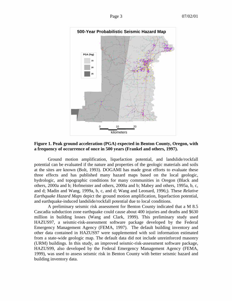
can be assessed on the basis of geologic, geophysical, geotechnical, hydrologic, andtopographic information. The probabilistic seismic hazard maps developed by GeomatrixConsultants, Inc. (1995) and the U.S. Geological Survey (Frankel and others, 1997)assess general ground shaking hazard on bedrock sites in Oregon. The OregonDepartment of Geology and Mineral Industries (DOGAMI) publication GMS-100 depictsprobabilistic ground shaking hazard in Oregon, including Benton County, at 500-, 1,000-,and 5,000-year return periods (Madin and Mabey, 1996). These maps provide a generalseismic hazard level for the State of Oregon. The ground motion design level in the Stateof Oregon 1998 edition of the Structural Specialty Code (Oregon Building CodesDivision, 1998) is based on these probabilistic seismic hazard assessments. Figure 1shows the peak ground acceleration on bedrock sites at a 500-year return interval inBenton County (Frankel and others, 1997). In addition, ground shaking from a greatCascadia subduction earthquake would be of long period and long duration (Clague andothers, 2000).
It is well documented that earthquake hazards are also affected by local geologic,hydrologic, and topographic conditions. Three phenomena generally will be induced byground shaking during a strong earthquake: (1) amplification of ground shaking by a “soft”soil column; (2) liquefaction of water-saturated sand, silt, or gravel, creating areas of“quicksand;” and (3) landslides, including rock falls and rock slides, triggered byshaking, even on relatively gentle slopes. The following are specific examples of theimpact of local conditions on earthquake hazard: (1) Amplified ground motion by near-surface soft soils resulted in great damage in Mexico City during the 1985 Mexicoearthquake (Seed and others, 1988). (2) Severe damage in the Marina district of SanFrancisco was also caused by amplified ground motion and by liquefaction during the1989 Loma Prieta earthquake (Holzer, 1994). (3) A large rock slide on the east side ofU.S. Highway 97 about 2.9 km south of Modoc Point, which hit a southbound vehicleand killed the driver, was induced by the September 1993 Klamath Falls earthquake(Keefer and Schuster, 1993).
Page 3 07/02/01
0
kilometers10 20
PGA (%g)
25
20
15
500-Year Probabilistic Seismic Hazard MapWILSON
STATE
GAME
MANAGEMENT
AREA
FOREST
REFUGE
R3
WILLIAM L. FINLEY
NATIONAL
WILDLIFE
FORESTS
PAUL
DUNN
STATE
RESEARCH
MCDONALD-DUNN
SIUSLAW
FOREST
NATIONAL
R1
FOREST
SIUSLAW
NATIONAL
Figure 1. Peak ground acceleration (PGA) expected in Benton County, Oregon, witha frequency of occurrence of once in 500 years (Frankel and others, 1997).
Ground motion amplification, liquefaction potential, and landslide/rockfallpotential can be evaluated if the nature and properties of the geologic materials and soilsat the sites are known (Bolt, 1993). DOGAMI has made great efforts to evaluate thesethree effects and has published many hazard maps based on the local geologic,hydrologic, and topographic conditions for many communities in Oregon (Black andothers, 2000a and b; Hofmeister and others, 2000a and b; Mabey and others, 1995a, b, c,and d; Madin and Wang, 1999a, b, c, and d; Wang and Leonard, 1996;). These RelativeEarthquake Hazard Maps depict the ground motion amplification, liquefaction potential,and earthquake-induced landslide/rockfall potential due to local conditions.
A preliminary seismic risk assessment for Benton County indicated that a M 8.5Cascadia subduction zone earthquake could cause about 400 injuries and deaths and $630million in building losses (Wang and Clark, 1999). This preliminary study usedHAZUS97, a seismic-risk-assessment software package developed by the FederalEmergency Management Agency (FEMA, 1997). The default building inventory andother data contained in HAZUS97 were supplemented with soil information estimatedfrom a state-wide geologic map. The default data did not include unreinforced masonry(URM) buildings. In this study, an improved seismic-risk-assessment software package,HAZUS99, also developed by the Federal Emergency Management Agency (FEMA,1999), was used to assess seismic risk in Benton County with better seismic hazard andbuilding inventory data.
Page 4 07/02/01
Water-Induced Landslide HazardThe term landslide denotes “the movement of a mass of rock, debris, or earth
down a slope” (National Research Council, 1996). It includes such phenomena as rockfalls, debris flows, earth slides, and others (National Research Council, 1996). Commonlandslide triggers include intense rainfall, rapid snowmelt, water-level changes, volcaniceruptions, and strong ground shaking during earthquakes (National Research Council,1996). Landslides triggered by water-related factors are complicated and can be classifiedin terms of state of activity (e.g., active vs. inactive landslides), distribution of activity(e.g., retrogressive vs. progressive landslides), and style of activity (e.g., complex orsingle landslides) (National Research Council, 1996). Types of landslides are largelydifferentiated by material properties, shear plane geometry, and triggering mechanisms.As a result, the analyses used to model or characterize different types of landslides varyand depend on site-specific conditions. Generally, landslide occurrence is determined bylocal topographic, hydrologic, and geologic conditions.
“An ideal landslide hazard map should provide information concerning the spatialand temporal probabilities of all anticipated landslide types within the mapped area, andalso include information about their types, magnitudes, velocities, and sizes” (NationalResearch Council, 1996). Landslide hazard mapping requires (1) a detailed inventory ofslope processes, (2) the study of those processes in relation to their environmental setting,(3) the analysis of conditioning and triggering factors, and (4) a representation of thespatial distribution of these factors (National Research Council, 1996). The level of detailin a landslide hazard map is dependent upon scale that can be national (less than 1:1million), regional (1:50,000 to 1:500,000), medium (1:25,000 to 1:50,000), or large(1:5,000 to 1:15,000). DOGAMI has published many landslide hazard maps at regionaland medium scales such as Environmental Geology of the Coastal Region of Tillamookand Clatsop Counties, Oregon (Schlicker and others, 1972), Environmental Geology ofInland Tillamook and Clatsop Counties, Oregon (Beaulieu, 1973), and landslidesusceptibility maps for the western portion of the Salem Hills, Marion County, and theeastern portion of the Eola Hills, Polk County (Harvey and Peterson, 1998 and 2000).
In the present study for Benton County, a GIS-based landslide hazard mappingtechnique was used to delineate landslide susceptibility triggered by the water-relatedfactors at regional scales (1:50,000 to 1:500,000) on the basis of (1) a landslide inventoryand (2) infinite slope modeling. In order to differentiate from earthquake-inducedlandslides, landslide hazard delineated in this project is called Water-Induced LandslideHazard.
The information from the water-induced landslide hazard mapping, and theseismic hazard and risk assessment will help local governments, land use planners, andemergency managers to prioritize areas for hazard mitigation and risk reduction. Thispreliminary report provides the results from relative seismic hazard mapping, buildinginventory investigation, seismic risk analysis, and landslide hazard mapping for BentonCounty.
Page 5 07/02/01
RELATIVE SEISMIC HAZARD MAPPINGThe first step in a relative earthquake hazard evaluation is the development of a
geologic model for the study area. The types of relative hazards present in a particulararea vary with the spatial distribution of geologic materials and other factors such astopography and hydrologic conditions. For ground motion amplification and liquefactionhazard analysis, the physical characteristics, spatial distribution, and thickness of theunconsolidated sediments overlying bedrock are of primary concern. For analysis ofearthquake-induced landslide hazard, slope may well be the most important factor, butbedrock geology (for slopes �25�) and the physical properties of the soils overlyingbedrock (for slopes 5��25�) are both significant in any dynamic slope-stability analysis.
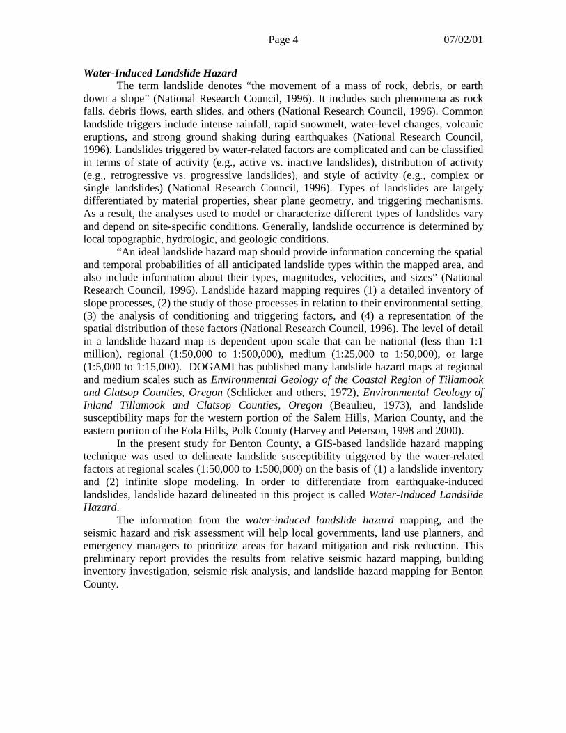
Surface and subsurface geologic, geophysical, geotechnical, and water well datawere used to generate a three-dimensional geologic model with the help of the GISsoftware MapInfo� and Vertical Mapper�. Bedrock and surficial geologic mapping inBenton County is based on Allison (1953), Vokes and others (1954), Baldwin (1955),Bela (1979), Walker and Duncan (1989), Walker and MacLeod (1991), and O’Connorand others (2000). The western part of Benton County lies within the Coast Range andassociated foothills, and comprises a thick sequence of Tertiary volcanic, sedimentary,and volcaniclastic rocks complicated by sills and dikes of basalt and gabbro (Figure 2).East of the Coast Range foothills lies the central Willamette Valley that has been infilledwith unconsolidated Quaternary sediments. The sediments comprise channel andfloodplain alluvium (Holocene), fine-grained Missoula Flood deposits (Pleistocene),fluvial sand and gravel deposits that predate the Missoula Floods of 12.7�15 ka, andolder fine-grained Pleistocene alluvium (Figure 2).
LEGEND
Pleistocene TerraceDeposits
Pleistocene MissoulaFlood Deposits
Holocene or PleistoceneLandslide deposits
Holocene Alluvium
Undifferentiated EoceneSedimentary andVolcaniclastic Rocks
Fault
Eocene SiletzRiver Volcanics
Oligocene Mafic Intrusives
ALBANY
Granger
VILLAGE
ADAIR
WILSON
STATE
GAME
MANAGEMENT
AREA
EstateCounty
FOREST
Lewisburg
Buchanan
Booneville
CreekDry
Greenberry
Shrock
Rickard
Bruce
Barclay
Jct.Bellfountain
REFUGE
MONROE
AlpineJct.
R3
Fern
WILLIAM L. FINLEY
NATIONAL
WILDLIFE
Bellfountain
Alpine
Glenbrook
Dawson
FORESTS
CORVALLIS
PAUL
DUNN
STATE
RESEARCH
MCDONALD-DUNN
Kopplein
Kings Valley
Hoskins
PHILOMATH
Wren
Russell
Alder
Har ris
Blodgett
SIUSLAW
Summit
FOREST
NATIONAL
R1
Alsea
FOREST
SIUSLAW
NATIONAL
20
kilometers
100
Figure 2. Generalized geologic map of Benton County.
Page 6 07/02/01
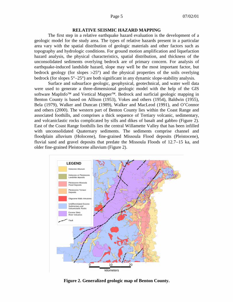
Characterization of the distribution and thickness of soil units in the centralWillamette Valley was accomplished using geologic maps, surface SH-wave refractiondata, geotechnical subsurface investigations, and water-well data. Geotechnicalinvestigations mainly conducted in the Corvallis area by the Oregon Department ofTransportation (ODOT) and various private consulting firms were also utilized in thisstudy. Water-well data were obtained from the Oregon Department of Water Resources(ODWR). Data from wells located by ODWR staff comprise the main basis for thegeologic model, but these data were augmented with ODWR data from wells located onlyto the quarter-quarter section (Figure 3). SH-wave refraction techniques (Wang andothers, 1998; Wang and others, 2000) were used to determine subsurface geologicmaterials and determine average shear-wave velocity for mapped stratigraphic units. SH-wave data were collected at 11 sites and largely focused around the Corvallis-Philomathurban areas (Figure 3). SH-wave data were processed on a personal computer using thecommercial software package SIP by Rimrock Geophysics, Inc. (version 4.1, 1995). Toprocess the data, refractions for each layer were identified, and then first-arrival timeswere picked and used to generate a shear-wave velocity model for the profile surveyed(see Table A-1 in Appendix A for a detailed shear-wave velocity profile at each site).
Figure 3. Location map of geotechnical boreholes, water well, and shear-wave sitesused for the Benton County geologic model.
Page 7 07/02/01
Ground shaking amplificationSoils and poorly consolidated sedimentary rocks overlying bedrock near the
surface can modify bedrock ground shaking caused by an earthquake. The physicalproperties, spatial distribution, and thickness of geologic materials above bedrock caninfluence the strength of shaking by increasing or decreasing it and/or by changing thefrequency of shaking. The method used to evaluate these modifications was developed bythe Federal Emergency Management Agency (FEMA) (Building Seismic Safety Council,1994). This method was adopted in the 1997 version of the Uniform Building Code(International Conference of Building Officials [ICBO], 1997) and will henceforth bereferred to as the UBC-97 methodology. This 1997 version of the Uniform Building Codewas adopted by the State of Oregon in October 1998 and became the State of Oregon1998 edition Structural Specialty Code.
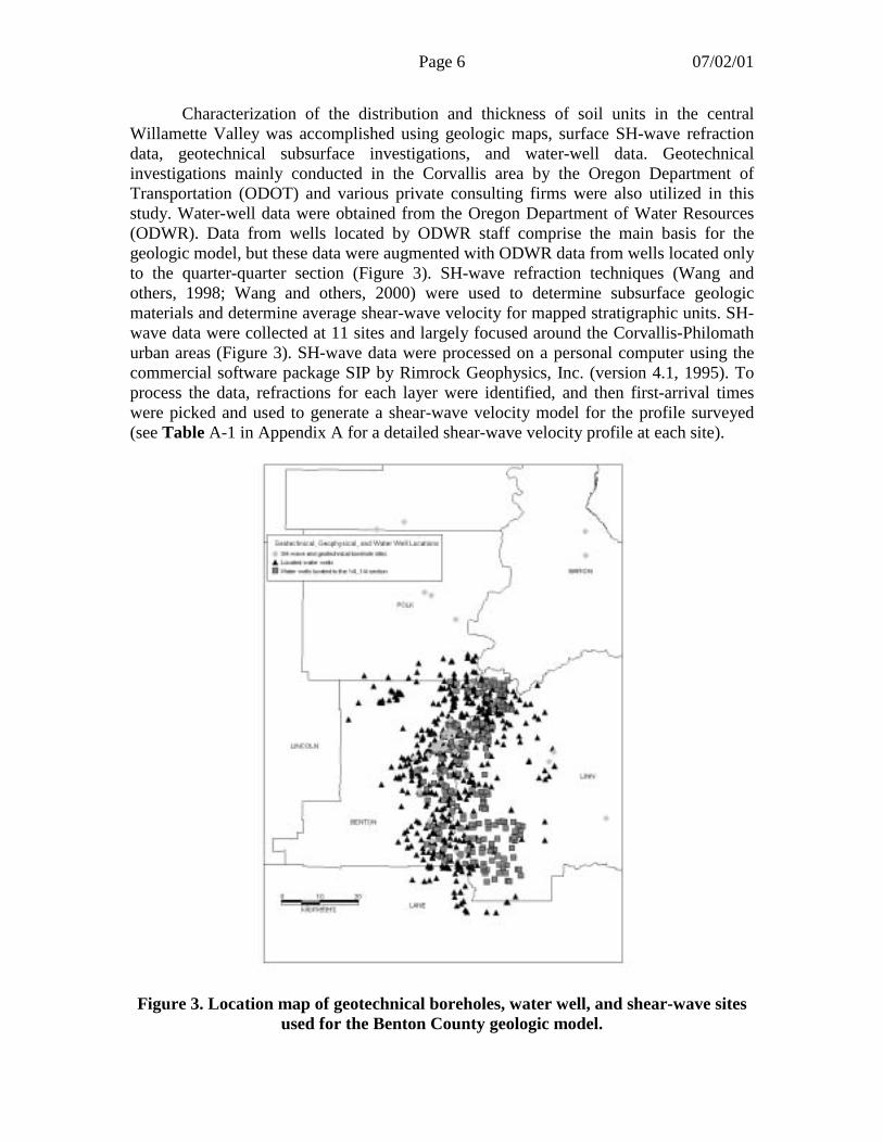
The UBC-97 methodology defines six soil categories that are based on averageshear-wave velocity, Standard Penetration Test (SPT) value, or undrained shear strengthin the upper 100 ft (30 m) of the soil column (Table 3). The six soil categories are HardRock (A), Rock (B), Very Dense Soil and Soft Rock (C), Stiff Soil (D), Soft Soil (E), andSpecial Soils (F). Category F soils are very soft soils that require site-specific evaluation.The ground motion amplification ranges from none (Hard Rock/A), to high (Soft Soil/Eand F).
Table 1. UBC-97 Soil Profile Types (ICBO, 1997).
Utilizing the UBC-97 methodology, a ground motion amplification map forBenton County was generated (Map 1). The Quaternary stratigraphy of the centralWillamette Valley in Benton County was differentiated into four main stratigraphic units:(1) Holocene channel and floodplain alluvium; (2) Pleistocene fine-grained flood depositsassociated with the Missoula Floods of 15�12.7 ka; (3) Pleistocene sand and graveldeposits that predate the Missoula Flood deposits; and (4) Pleistocene fine-grainedalluvium that predates all of those soils. These geologic units and their average shear-wave velocity and liquefaction susceptibility are listed in Table 2. Because SH-wavetesting provided data for bedrock from only two sites, data from ten nearby sites reportedin Wang and Madin (1999c, d) with bedrock units comparable to those exposed inBenton County were also used to determine the average shear-wave velocity for bedrock.
Average Soil Properties for Top 30 m (100 feet)
Soil Type Soil Name Shear-waveVelocity,Vs (m/s)
Standard PenetrationTest, N (blows/foot)
UndrainedShear Strength
su (kPa)SA Hard Rock >1,500SB Rock 760 to 1,500 - -
SC
Very DenseSoil and Soft
Rock360 to 760 >50 >100
SD Stiff Soil 180 to 360 15 to 50 50 to 100SE Soft Soil <180 <15 <50SF Soil Requiring Site-specific Evaluation
Page 8 07/02/01
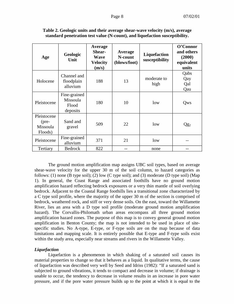
Table 2. Geologic units and their average shear-wave velocity (m/s), averagestandard penetration test value (N-count), and liquefaction susceptibility.
Age GeologicUnit
AverageShear-Wave
Velocity(m/s)
AverageN-count
(blows/foot)
Liquefactionsusceptibility
O’Connorand others
(2000)equivalent
units
HoloceneChannel andfloodplainalluvium
188 13 moderate tohigh
QabsQayQalQau
Pleistocene
Fine-grainedMissoula
Flooddeposits
180 10 low Qws
Pleistocene(pre-
MissoulaFloods)
Sand andgravel 509 22 low Qg2
Pleistocene Fine-grainedalluvium 371 21 low --
Tertiary Bedrock 822 -- none --
The ground motion amplification map assigns UBC soil types, based on averageshear-wave velocity for the upper 30 m of the soil column, to hazard categories asfollows: (1) none (B type soil); (2) low (C type soil); and (3) moderate (D type soil) (Map1). In general, the Coast Range and associated foothills have no ground motionamplification hazard reflecting bedrock exposures or a very thin mantle of soil overlyingbedrock. Adjacent to the Coastal Range foothills lies a transitional zone characterized bya C type soil profile, where the majority of the upper 30 m of the section is comprised ofbedrock, weathered rock, and stiff or very dense soils. On the east, toward the WillametteRiver, lies an area with a D type soil profile (moderate ground motion amplificationhazard). The Corvallis-Philomath urban areas encompass all three ground motionamplification hazard zones. The purpose of this map is to convey general ground motionamplification in Benton County; the map is not intended to be used in place of site-specific studies. No A-type, E-type, or F-type soils are on the map because of datalimitations and mapping scale. It is entirely possible that E-type and F-type soils existwithin the study area, especially near streams and rivers in the Willamette Valley.
LiquefactionLiquefaction is a phenomenon in which shaking of a saturated soil causes its
material properties to change so that it behaves as a liquid. In qualitative terms, the causeof liquefaction was described very well by Seed and Idriss (1982): “If a saturated sand issubjected to ground vibrations, it tends to compact and decrease in volume; if drainage isunable to occur, the tendency to decrease in volume results in an increase in pore waterpressure, and if the pore water pressure builds up to the point at which it is equal to the

Page 9 07/02/01
overburden pressure, the effective stress becomes zero, the sand loses its strengthcompletely, and it develops a liquefied state.”
Soils that liquefy tend to be young, loose, granular soils that are saturated withwater (National Research Council, 1985). Unsaturated soils will not liquefy, but they maysettle. If an earthquake induces liquefaction, several things can happen: (1) the liquefiedlayer and everything lying on top of it may move downslope; (2) the liquefied layer mayoscillate with displacements large enough to rupture pipelines, move bridge abutments, orrupture building foundations; and (3) light objects, such as underground storage tanks, canfloat toward the surface, and heavy objects, such as buildings, can sink. Typicaldisplacements can range from centimeters to meters. Thus, if the soil at a site liquefies,the total damage resulting from an earthquake can be dramatically increased from thatcaused by shaking alone.
Liquefaction hazard potential was first evaluated on the basis of age andengineering properties of the geologic unit and hydrologic conditions. Youd and Perkins(1978) found that the liquefaction potential for different sediments is related to age anddepositional environment. Table 3 summarizes the liquefaction potential for severalcontinental deposits (Youd and Perkins, 1978).
A further evaluation was performed for those geologic units with moderate tohigh liquefaction susceptibility and was based on the age and depositional environmentsin terms of ground shaking strength, SPT or shear-wave velocity, and the depth to watertable (Seed and Idriss, 1971; Andrus and Stokoe, 1996). Andrus and Stokoe (1996) foundthat soils with a shear-wave velocity of less than 200 m/s have liquefaction potential.Hence, Holocene alluvium (Vs = 188 m/s) is considered to be the unit susceptible toliquefaction (Table 2).
Table 3. Estimated Susceptibility of Continental Deposits to Liquefaction (modifiedfrom Youd and Perkins, 1978).
Likelihood that Cohesionless Sediments, When Saturated,Would Be Susceptible to Liquefaction (by Age of Deposit)
Type of deposit <500 yr Holocene Pleistocene Pre-Pleistocene
River channel Very high High Low Very lowFlood Plain High Moderate Low Very lowAlluvial fan andPlain
Moderate Low Low Very low
Lacustrine andplaya
High Moderate Low Very low
Colluvium High Moderate Low Very lowTalus Low Low Very low Very lowTuff Low Low Very low Very lowResidual soils Low Low Very low Very low
Liquefaction hazard assignments for each geologic unit based on age, depositionalenvironment, and average shear-wave velocity are listed in Table 2. The liquefactionpotential hazard map for Benton County is illustrated on Map 2. As depicted on the map,areas with moderate to high liquefaction susceptibility, comprised of Holocene alluvium,are concentrated along the Willamette River, Coast Range tributaries, and major stream
Page 10 07/02/01
valleys within the Coast Range. Pleistocene terrace and Missoula Flood deposits wereassigned a low liquefaction susceptibility hazard.
Earthquake-induced landslideThe earthquake-induced landslide hazard map is based on state-of-practice
analysis for slope stability; empirical correlations of slope stability with engineeringproperties of materials; and the characterization of local topography, engineeringgeology, and hydrology with GIS tools.
Because failure mechanisms tend to vary with slope steepness, each grid cell wasassigned to one of three slope categories, and different analytical techniques were appliedto each category. Slopes between 0º and 10º were assigned a very low slope instabilityhazard because it was found that the slopes in this range have very low susceptibility forearthquake-induced failure (Jibson and others, 1998; McCrink and Real, 1996). Steepslopes (>25º), which most commonly fail by rock falls, rock slides, and debris slides(Keefer, 1984), are analyzed by means of an empirical relationship that relates slopestability to degree of weathering, strength of cementation, spacing and openness of rockfractures, and hydrologic conditions (Keefer, 1984, 1993). Moderate slopes (10º�25º)produce larger numbers of rotational slumps and translational block slides in soil (Keefer,1984). Slopes between 10º and 25º were analyzed by means of a slope stability analysisbased on slope inclination, engineering properties of soil units, and hydrologicconditions.
Existing LandslidesMotion of existing landslides is highly variable, ranging from active movement to
stable. Although most earthquake-induced landslides occur in materials not previouslyinvolved in sliding (Keefer, 1984), it requires site-specific studies to understand thenature of any existing landslide. Therefore it was assumed that the slip planes of mappedlandslides are at reduced shear strength of unknown value and that the slide masses areinherently unstable under earthquake loading. Existing landslides are conservativelyassigned to the high hazard category, and no analytical techniques were applied. Themapping of existing landslides is described in detail in the Water-induced LandslideHazard section.
Steep Slopes (>25º)Slopes >25º are particularly vulnerable to bedrock failures. Keefer (1984, 1993)
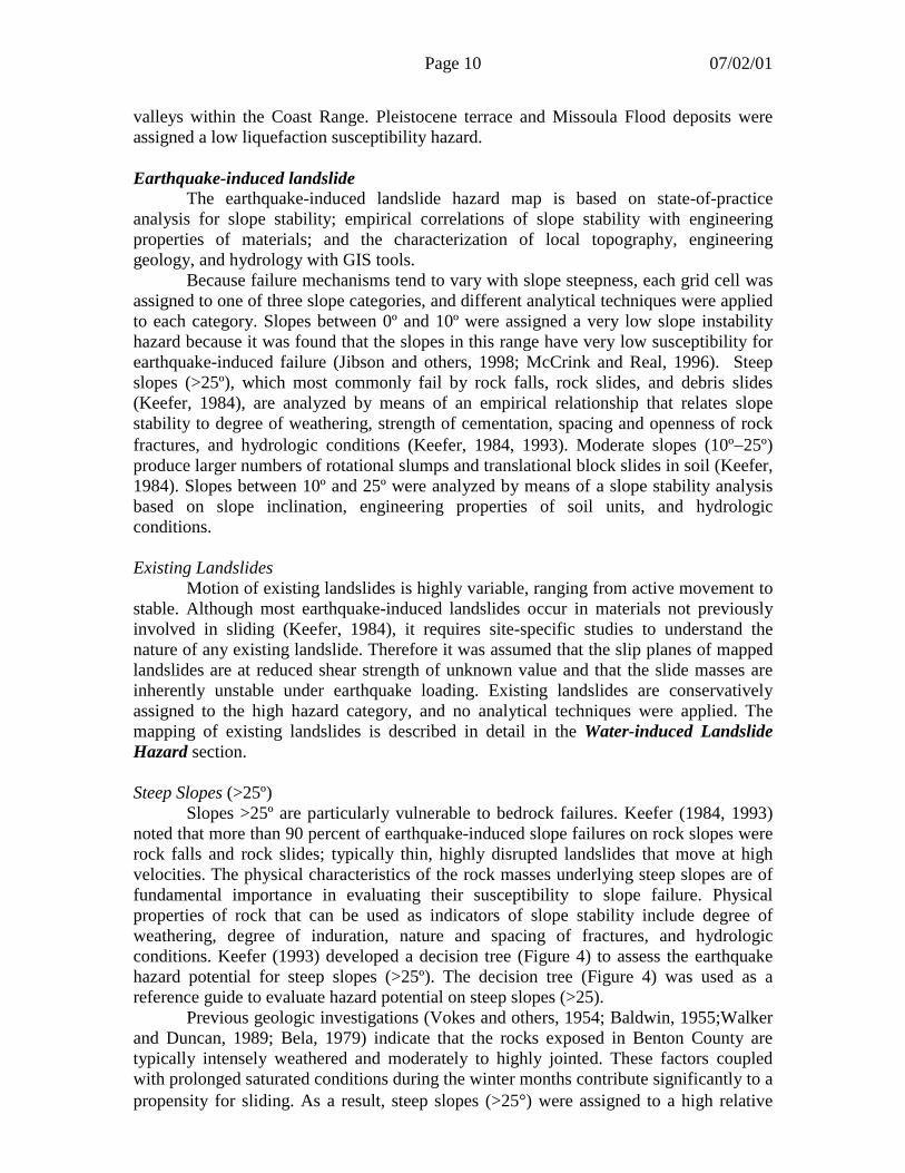
noted that more than 90 percent of earthquake-induced slope failures on rock slopes wererock falls and rock slides; typically thin, highly disrupted landslides that move at highvelocities. The physical characteristics of the rock masses underlying steep slopes are offundamental importance in evaluating their susceptibility to slope failure. Physicalproperties of rock that can be used as indicators of slope stability include degree ofweathering, degree of induration, nature and spacing of fractures, and hydrologicconditions. Keefer (1993) developed a decision tree (Figure 4) to assess the earthquakehazard potential for steep slopes (>25º). The decision tree (Figure 4) was used as areference guide to evaluate hazard potential on steep slopes (>25).
Previous geologic investigations (Vokes and others, 1954; Baldwin, 1955;Walkerand Duncan, 1989; Bela, 1979) indicate that the rocks exposed in Benton County aretypically intensely weathered and moderately to highly jointed. These factors coupledwith prolonged saturated conditions during the winter months contribute significantly to apropensity for sliding. As a result, steep slopes (>25�) were assigned to a high relative

Page 11 07/02/01
hazard category. The potential ramifications associated with long-duration groundshaking from a Cascadia subduction earthquake (Clague and others, 2000) were alsotaken into consideration in the hazard assignment for steep slopes.
Steeperthan 25�
Low
?
Intenselyweathered?
Poorl yindurated ?EXTREMELY
HIGH
VERYHIGH
Fissures open ?
Fis sures closed spaced
?
HIGH
Wet ?HIGH
Fissures closed spaced ?
MODERATE
LOW
ADJUSTMENTSExcept for slope units ra ted LOW,increase s usceptibi lity rat ing byone grade i f l ocal topographi c rel ief is greate r than 2000m (6,600ft .), decrease suscept ibili tyrat ing by one grade if M�6.5 and slope unit is vege ta ted.
OTHER TYPE OF SLOPES SUS CEPTIBILITYEngineered slopes wi th reiforced reta ini ngwal ls or re ta ining st ruc tures well anchored
Pre-exist ing landslide depos its (inc ludingthose on slope gent le r t han 25�)
LOW
HIGH
Figure 4. Decision tree for evaluation of earthquake-induced rock slopehazard (Keefer, 1993).
Moderate Slopes (10º to 25º)
The stability analysis for moderate slopes is based on the dynamic slope stabilityanalysis of Newmark (1965) as verified and extended to regional-scale work by Wilsonand Keefer (1983, 1985), Wieczorek and others (1985), Jibson (1993, 1996), and Jibsonand Keefer (1993). The procedure to assign hazard categories takes several steps. First,using infinite slope analysis, the static factor of safety is calculated for each grid element.This factor of safety is then used to calculate the critical acceleration, which is theacceleration required to overcome friction and initiate sliding in the soil mass. Thecritical acceleration is then used in conjunction with earthquake input parameters tocalculate the total displacement that is expected to occur during the design earthquake.This procedure has been used in Oregon by Black and others (2000a, b), Hofmeister andothers (2000a, b), Wang and Wang (2000), and Wang and others (2001).
The factor of safety (FS) calculation for a static infinite slope model is discussedin detail in the next section entitled Water-induced Landslide Hazard. The criticalacceleration (ac) in terms of g can be obtained through an equation developed byNewmark (1965):
ac= (FS-1) sin �
where FS is the static factor of safety and � is the thrust angle.Newmark displacement (DN) is a function of critical acceleration and Arias
Intensity according to the following empirical regression equation (Jibson, 1993):
log DN = 1.460 log Ia - 6.642ac + 1.546
Page 12 07/02/01
where Ia is the Arias Intensity in meters per second. The Arias Intensity (Ia) canbe estimated by a relationship developed by Wilson and Keefer (1985):
log Ia = M – 2 log R – 4.1
where M is the moment magnitude of a design earthquake and R is the earthquakesource-to-site distance in kilometers. A M 8.5 subduction zone earthquake approximately20 km offshore was used for slope stability analysis in this project. This is approximatelyequivalent to an Arias Intensity (Ia) of 3.9 m/s.
Finally, the total displacement was used to assign that element of slope to anearthquake-induced slope instability hazard category. Hazard categories used for thisproject were:
Low Displacement <10 cm (3.9 in.)Moderate Displacement 10 -100 cm (3.9-39 in.)High Displacement > 100 cm (39 in.)
The results from the analyses for the three slope categories and the mappedlandslide layer were combined to construct the earthquake-induced landslide hazardpotential map for Benton County (Map 3).
WATER-INDUCED LANDSLIDE HAZARDCommon landslide triggers include intense rainfall, rapid snowmelt, water-level
changes, volcanic eruptions, and strong ground shaking during earthquakes (NationalResearch Council, 1996). In this study, we evaluated landslides that are triggered bywater-related factors and delineate landslide susceptibility for Benton County at aregional scale (1:50,000 to 1:500,000) based on a landslide inventory and infinite slopemodeling. This water-related landslide hazard differs from the earthquake-inducedlandslide hazard mainly in the type of failure and the triggering mechanism.
Landslide InventoryThe first part of the slope stability analysis performed as part of this investigation
involved identifying existing landslides through aerial photo interpretation, availablelandslide data, and limited field investigations in the Corvallis area.
Benton CountyLandslides mapped from previous investigations were digitized and utilized in
this study. Bela (1979) mapped landslide deposits as part of an assessment of geologichazards for eastern Benton County. Landslide deposits mapped by Bela (1979) at a scaleof 1:24,000 in the Lewisburg, Corvallis, Greenberry, and Monroe 7.5' quadrangles weretransferred by inspection from paper copies into MapInfo using 7.5' Digital RasterGraphic (DRG) topographic base maps. Additional landslide deposits, outside the above-mentioned 7.5' quadrangles, were mapped by Bela (1979) at a scale of 1:62,500. Theseslide deposits were also transferred by inspection to 7.5' DRG topographic base maps.However, it must be noted that the transfer of these landslide deposits was complicatedby base maps at different horizontal scales (1:24,000 vs. 1:62,500) as well as variouscontour intervals.
Page 13 07/02/01
Additional landslide deposits were compiled from the Salem 1� by 2� geologicquadrangle mapped by Walker and Duncan (1989); a digitized soil survey of the Alseaarea by Corliss (1973); and a digitized database of slope failures compiled by Hofmeister(2000). In an effort to identify additional large, deep-seated landslides, aerial photocoverages for Benton County from 1948 (1:20,000), 1970 (1:20,000), and 1994(1:24,000) were inspected using a stereo scopic viewers. Large areas interpreted to reflectslide deposits based on topographic/geomorphic expression were transferred directly intoMapInfo with the use of Digital Raster Graphic (DRG) base maps. No efforts were madeto field-check any of the potential landslide deposits mapped during this portion of theinvestigation.
Corvallis-Philomath Urban AreasA more detailed slide map for within and surrounding the Corvallis-Philomath
urban growth boundary was also compiled (Figure 5). Landslides were compiled fromgeologic mapping by Bela (1979), a digital soil map of the MacDonald-Dunn ResearchForest, and exhaustive photogeologic mapping from aerial photos. Forest cover in thearea makes it very difficult to see subtle landforms associated with landslides. In order to“see through” the trees, a time-series of photographs was examined, in hopes of catchingmost of the area without tree cover due to periodic logging or clearing for agriculture ordevelopment. Photo coverages of the area from 1936, 1944, 1948, 1956, 1963, 1970,1978, 1990, and 1998 were examined in stereo, and any areas of slide topography weretransferred by inspection to MapInfo, with Digital Orthophoto images as a base maps.
Very limited field checking was done for most of the larger slides within theurban area. The field checking was limited to driving through the affected areas, becausemost of the larger slides are on private property, and there was not sufficient time toobtain permission to field-check offroad areas. The larger slides that are on the map arethose for which plausible evidence of sliding was observed in the field check.
A total of 110 possible slides was mapped in the Corvallis-Philomath study area(Figure 5). The slides range in size from a fraction of an acre to over 50 acres, and mostare outside the Corvallis and Philomath Urban Growth Boundaries. Figure 5 is a slopemap of the study area derived from the 10-m Digital Elevation Model (DEM) resampledto 50 m. Clearly, mostof the steep slopes are in the hills surrounding the urban growthboundaries. Most of the smaller slides are likely to be debris flows or soil flows,involving rapid failure of saturated soil or colluvium. Most of the larger slides are likelyto be deeper seated rotational slumps or translational block slides, involving themovement of soil, colluvium, and underlying bedrock. One particularly notable slidecomplex occurs at Vineyard Mountain, at the north end of the study area. Bela (1979)shows some large slide areas here, and numerous small shallow slides were reported andinvestigated in conjunction with development of the area. This geotechnical studyconcluded that the abundant small slides in the area were occurring in thin deposits ofsoil and colluvium. Inspection of the historic air photos in this study suggests that thesesmall slides were occurring on a much larger, deep-seated bedrock slide mass.

Page 14 07/02/01
Figure 5. Slope map of the Corvallis-Philomath Urban Growth Boundaries andsurrounding area with mapped landslide deposits.
LimitationsThere are several significant limitations to both the countywide landslide
inventory and the more detailed inventory of the Corvallis-Philomath urban area . First,for many slides, extensive field checking should be done to confirm the presence of aslide. Second, many parts of the area were forested during the entire span covered by thephoto time series. It was not possible, within the scope of this project, to map the areaswhere forest cover may significantly obscure the features. Hence, many areas without
Page 15 07/02/01
mapped slides may indeed have slides that were not visible given the methods of thisreport. There was also no effort made to distinguish between the types of slides mapped.This is important, because in the case of debris flows, the hazard is likely to be in therunout zone, with lesser hazard in the area from which the slide originates. In the case ofdeep-seated slides, there may be less risk of rapid, life-threatening motion but a high riskof slow movement with incremental damage to structures.
Model AnalysisThe factor of safety (FS) for an infinite slope in material having both frictional
and cohesive strength is given by:
��
���
sintancos'�
�cFS
where c soil cohesion�’ effective normal stress� slope angle� soil friction angle� total normal stress
To implement the slope stability analysis, we used the GIS programs MapInfo andVertical Mapper. A Digital Elevation Model (DEM) for Benton County with a 10-m gridspacing was acquired from the U.S. Geological Survey (USGS). Vertical Mapper wasused to calculate slope angle for each grid cell from the USGS DEM. Digitized soil mapsand relational soil property databases for the Benton County area (Knezevich, 1975),Alsea area (Corliss, 1973), Lane County (Patching, 1987), and Linn County (Langridge,1987) were obtained from the National Resource Conservation Service (NRCS) through aSSURGO data download.
The factor of safety calculation specifically requires slope angle, depth to thefailure plane, thickness of soil mass, unit weights for each soil layer, porosity for eachsoil layer, depth to the ground water table, and material strength properties (cohesion andinternal friction angle) along the basal failure plane. Slope angle was calculated usingVertical Mapper with the 10-m DEM and the output values were stored at the same 10-mgrid spacing as the DEM. The remainder of the input parameters were grouped accordingto soil polygon boundaries, using engineering properties contained in the NRCSrelational soil databases. In particular, the relational soil databases contain information onUnified Soil Classification System (USCS) designation, bulk density, plasticity index,clay content, average thickness for each soil layer, and depth to bedrock for each soil unitif encountered in the depth of the soil survey. The data within the NRCS databases andthe following assumptions were used for the calculation of the total and effective stressesfor each soil unit (Black and others, 2000a and b; Hofmeister and others, 2000).
Depth to failure plane: The depth to failure plane was assumed to occur at the soil-bedrock interface if listed in the soils database. Depth tobedrock was listed in the NRCS database as a range, thelowest value of which was used in the stability analysis. Ifbedrock was not encountered during the depth of survey,the failure plane was assumed to be at a depth of 2.44 m(8 ft).
Page 16 07/02/01
Thickness of soil units: Where bedrock was not encountered in the depth of thesurvey, the properties of the lowest reported soil layer wereassumed to extend to the depth of the failure plane.
Density: Soil densities were reported as a range of “moist bulkdensity.” Given that the samples were collected duringsummer field work (U.S. Department of Agriculture, 1996)when the soils were thoroughly dried, it was assumed thatthe dry bulk density for factor-of-safety calculations wasthe average of the reported “moist bulk density” range.
Porosity: Porosity values were assigned according to the dominantUSCS soil type for each layer listed in the NRCS database.Values are listed in Table 4 and were largely inferred fromcharts listing typical soil index properties in NavalFacilities Engineering Command (NFEC) (1986).
Unit weight: Unit weights were calculated assuming 100% saturation.
Depth to water table: If the depth was not reported, the water table was assumedto be at the surface consistent with other assumptions ofsaturated conditions.
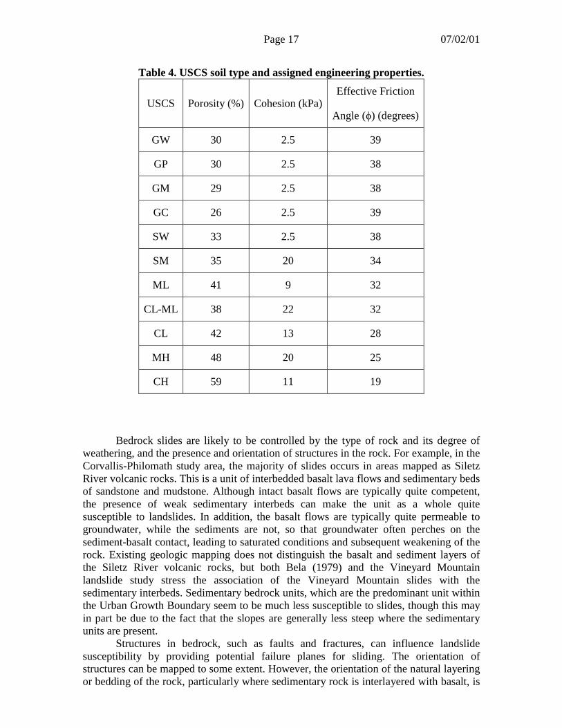
Soil strength properties were assigned according to the dominant USCS soil listedin the lowest layer of each map unit recorded in the NRCS databases. In the absence oflaboratory data for specific soils and due to the highly variable nature of geologicmaterials, the cohesion values used for SM, ML, CL-ML, CL, MH, and CH soils aretypical saturated values reported by Driscoll (1979) (Table 4). GW, GP, GM, GC, andSW soils were assigned a lower cohesion value of 2.5 kPa to account for apparentcohesion inferred from modeling trials, part of which may also reflect root strength.Friction angles were assigned on the basis of USCS classification according to typicalstrength properties listed in Driscoll (1979) and USDA (1981) (Table 4).
The input parameters for the factor-of-safety calculation were grouped accordingto soil polygon boundaries. Hence, each soil polygon has a unique identifier, a map unitsymbol in this case, as well as values for total and effective stress, cohesion, and frictionangle (Appendix A). The slope grid, with a 10-m spacing, was then updated with the totaland effective stress, cohesion, and friction angle assigned to the soil polygon that theslope point falls within. As a result, all parameters necessary for the factor-of-safetycalculation were stored in one database. The static factor of safety for each grid cell couldthen be calculated using standard MapInfo database capabilities.
Factors which control the distribution of slidesThe nature of the material making up a slope is an important factor. The thickness
and engineering properties of soil, colluvium, and weathered rock; shear strength andstructure of the bedrock; and hydrologic conditions are also very important. In general itis very difficult and time consuming to map the thickness of soil and colluvium, but thethickness is typically greater in the bottoms of drainages than on open slopes or ridges.This is reflected in the relatively common association of slides with minor drainages.
Page 17 07/02/01
Table 4. USCS soil type and assigned engineering properties.
USCS Porosity (%) Cohesion (kPa)Effective Friction
Angle (�) (degrees)
GW 30 2.5 39
GP 30 2.5 38
GM 29 2.5 38
GC 26 2.5 39
SW 33 2.5 38
SM 35 20 34
ML 41 9 32
CL-ML 38 22 32
CL 42 13 28
MH 48 20 25
CH 59 11 19
Bedrock slides are likely to be controlled by the type of rock and its degree of
weathering, and the presence and orientation of structures in the rock. For example, in theCorvallis-Philomath study area, the majority of slides occurs in areas mapped as SiletzRiver volcanic rocks. This is a unit of interbedded basalt lava flows and sedimentary bedsof sandstone and mudstone. Although intact basalt flows are typically quite competent,the presence of weak sedimentary interbeds can make the unit as a whole quitesusceptible to landslides. In addition, the basalt flows are typically quite permeable togroundwater, while the sediments are not, so that groundwater often perches on thesediment-basalt contact, leading to saturated conditions and subsequent weakening of therock. Existing geologic mapping does not distinguish the basalt and sediment layers ofthe Siletz River volcanic rocks, but both Bela (1979) and the Vineyard Mountainlandslide study stress the association of the Vineyard Mountain slides with thesedimentary interbeds. Sedimentary bedrock units, which are the predominant unit withinthe Urban Growth Boundary seem to be much less susceptible to slides, though this mayin part be due to the fact that the slopes are generally less steep where the sedimentaryunits are present.
Structures in bedrock, such as faults and fractures, can influence landslidesusceptibility by providing potential failure planes for sliding. The orientation ofstructures can be mapped to some extent. However, the orientation of the natural layeringor bedding of the rock, particularly where sedimentary rock is interlayered with basalt, is
Page 18 07/02/01
more important. If the layers are tilted parallel to the slope (as is the case, e.g., atVineyard Mountain), they are much more prone to slide. This situation is called a dipslope, and it may be possible to map areas that are likely to have this condition withexisting geologic data and GIS techniques.
Bela (1979) noted the importance of another bedrock condition that results inlandslide occurrence. Dikes and sills of basalt and gabbro, both relatively strong rock, arecommonly found injected into mudstone and sandstone units (Eocene Tyee Formation) inthe area. Slides commonly occur along the boundaries between these two rock types. Thehigher peaks within Benton County such as Marys Peak, Grass Mountain, and FlatMountain are cored by the above-mentioned Oligocene intrusives. These peaks arecommonly flanked by large, deep-seated landslide deposits most likely reflecting apropensity for sliding along the boundaries of intrusive bodies.
Landslide hazard assignmentThe activity of existing landslides is extremely variable, ranging from active
movement to stability. Site-specific investigations are required to characterize the natureof any existing landslide. The shear planes of mapped landslides are assumed to be at areduced shear strength of unknown value. Consequently, existing landslides areconservatively assigned to a high hazard rating, and no analytical techniques were usedfor this portion of the slope stability analysis.
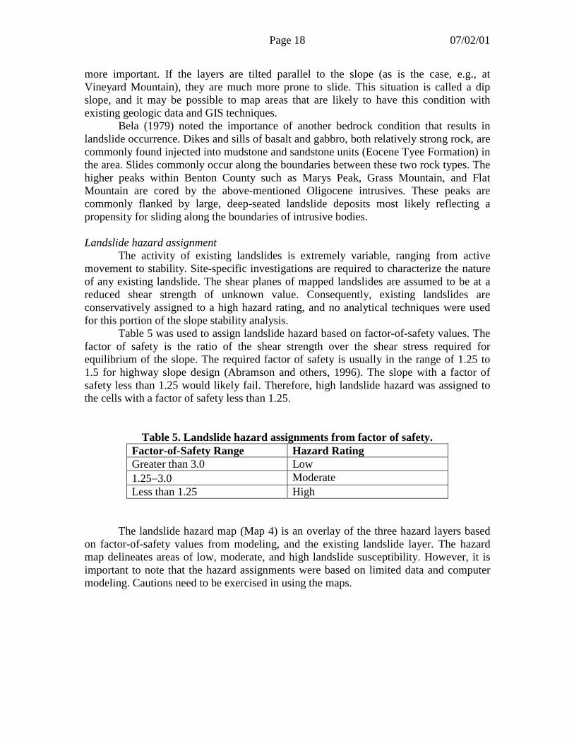
Table 5 was used to assign landslide hazard based on factor-of-safety values. Thefactor of safety is the ratio of the shear strength over the shear stress required forequilibrium of the slope. The required factor of safety is usually in the range of 1.25 to1.5 for highway slope design (Abramson and others, 1996). The slope with a factor ofsafety less than 1.25 would likely fail. Therefore, high landslide hazard was assigned tothe cells with a factor of safety less than 1.25.
Table 5. Landslide hazard assignments from factor of safety.Factor-of-Safety Range Hazard RatingGreater than 3.0 Low1.25�3.0 ModerateLess than 1.25 High
The landslide hazard map (Map 4) is an overlay of the three hazard layers basedon factor-of-safety values from modeling, and the existing landslide layer. The hazardmap delineates areas of low, moderate, and high landslide susceptibility. However, it isimportant to note that the hazard assignments were based on limited data and computermodeling. Cautions need to be exercised in using the maps.
Page 19 07/02/01
SEISMIC RISK ASSESSMENTSound earthquake risk reduction plans should imcorporate detailed risk
assessment based on the best available data. DOGAMI completed a seismic riskassessment for the State of Oregon (Wang and Clark, 1999), utilizing the earthquake riskassessment software HAZUS97 from the Federal Emergency Management Agency(NIBS, 1997), and statewide hazard information (Wang and Clark, 1999). Preliminaryseismic risk information for Benton County was included in the statewide risk assessment(Wang and Clark, 1999). The information used in these rough regional studies used thedefault building data in HAZUS97 and statewide seismic hazard data.
In this study, seismic risk assessment for Benton County was performed with theseismic hazard maps developed in this project and HAZUS99 software by FEMA (NIBS,1999). We augmented the building inventory provided in HAZAUS99 for the county byextrapolating available building data from the city of Corvallis and Benton County andtargeted field surveys (Rad and Hasenberg, 2000).
Building Inventory The default building inventory of HAZUS99 was derived from a nationwide database
analysis (NIBS 1999). However, this default inventory might not reflect the actualcharacteristics of building stock in Benton County. With support from DOGAMI, adetailed building survey was conducted in downtown Corvallis by Portland StateUniversity (PSU) (Rad and Hasenberg, 2000). The building inventory contained inHAZUS99 was augmented with survey data and available building information fromvarious sources (Rad and Hasenberg, 2000). Rad and Hasenberg (2000) concluded that:
(1) Total single-family residential building area from the project data was 22%larger than the HAZUS default data. This is largely due to the fact that certaintracts are growing rapidly and the survey data were much more up to date thanthe HAZUS default data.
(2) Building quantities for the Oregon State University campus were greatlyunderestimated in the HAZUS default data.
(3) The total commercial building areas are within 4% between the project dataand HAZUS default data. However, the breakdowns into specific categoriesare very different. The project data show nearly twice as much retailcommercial areas and about half as much office space as the HAZUS defaultdata.
(4) Industrial buildings were underestimated by the HAZUS default data, largelydue to expansion of the Hewlett Packard Company, Inc., campus.
The HAZUS99 default data (FEMA, 1999) categorized the buildings in BentonCounty into the “low code” seismic code category with data in both the “to code” and“inferior to code” divisions. For the mapping schemes developed in this study, buildingsbuilt prior to 1975 were put in the “low code – inferior” category and buildings built in1975 and later were put in the “moderate code – to code” category. Oregon has been inseismic zone 2 or greater since 1975.
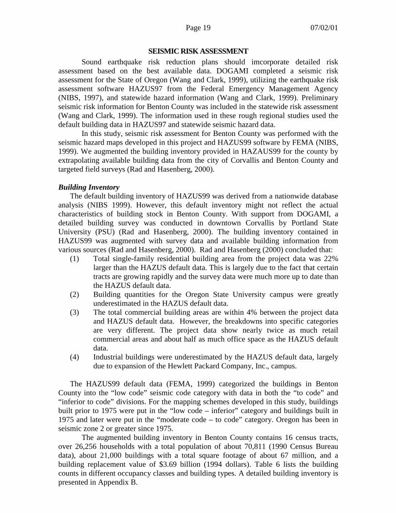
The augmented building inventory in Benton County contains 16 census tracts,over 26,256 households with a total population of about 70,811 (1990 Census Bureaudata), about 21,000 buildings with a total square footage of about 67 million, and abuilding replacement value of $3.69 billion (1994 dollars). Table 6 lists the buildingcounts in different occupancy classes and building types. A detailed building inventory ispresented in Appendix B.
Page 20 07/02/01
Table 6. Building counts in different occupancy classes and building type in BentonCounty.
Occupancy Classes Building TypeClass Count Type Count
Residential 19,096 Wood 17,050Commercial 772 Steel 457
Industrial 134 Concrete 291Agriculture 653 Precast Concrete 266
Religion 73 Reinforced Masonry 389Government 67 Unreinforced Masonry 290Education 198 Mobile Homes 2,249
Total 20,993 Total 20,992
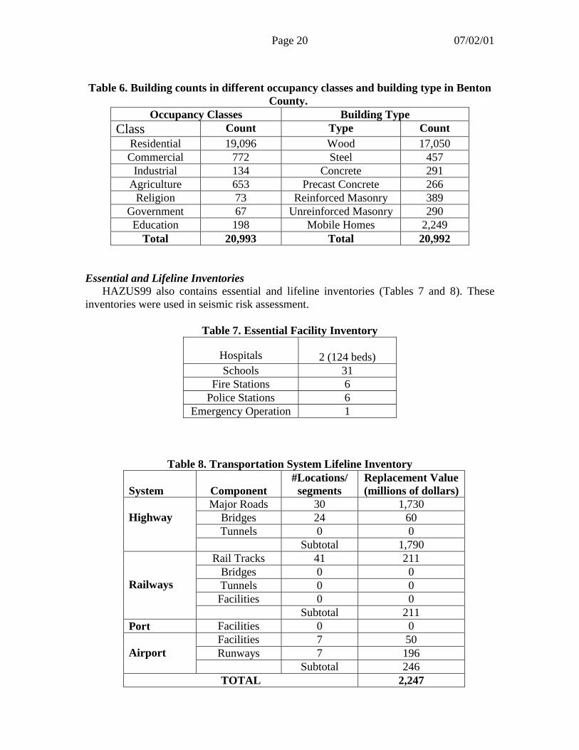
Essential and Lifeline InventoriesHAZUS99 also contains essential and lifeline inventories (Tables 7 and 8). These
inventories were used in seismic risk assessment.
Table 7. Essential Facility Inventory
Hospitals 2 (124 beds)Schools 31
Fire Stations 6Police Stations 6
Emergency Operation 1
Table 8. Transportation System Lifeline Inventory
System Component#Locations/
segmentsReplacement Value(millions of dollars)
Major Roads 30 1,730Bridges 24 60Tunnels 0 0
Highway
Subtotal 1,790Rail Tracks 41 211
Bridges 0 0Tunnels 0 0Facilities 0 0
Railways
Subtotal 211Port Facilities 0 0
Facilities 7 50Runways 7 196Airport
Subtotal 246TOTAL 2,247
Page 21 07/02/01
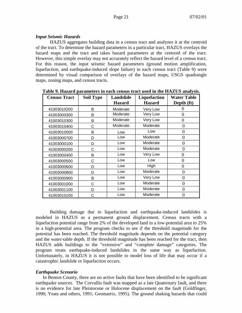
Input Seismic Hazards HAZUS aggregates building data in a census tract and analyzes it at the centroid
of the tract. To determine the hazard parameters in a particular tract, HAZUS overlays thehazard maps and the tract and takes hazard parameters at the centroid of the tract.However, this simple overlay may not accurately reflect the hazard level of a census tract.For this reason, the input seismic hazard parameters (ground motion amplification,liquefaction, and earthquake-induced slope failure) in each census tract (Table 9) weredetermined by visual comparison of overlays of the hazard maps, USGS quadranglemaps, zoning maps, and census tracts.
Table 9. Hazard parameters in each census tract used in the HAZUS analysis.Census Tract Soil Type Landslide
HazardLiquefaction
HazardWater Table
Depth (ft)41003010200 B Moderate Very Low 0 41003000300 B Moderate Very Low 0 41003010300 B Moderate Very Low 0 41003010400 C Moderate Moderate 041003010500 B Low Low 041003000700 D Low Moderate 041003000100 D Low Moderate 041003000200 C Low Moderate 041003000400 B Low Very Low 0 41003000500 C Low Low 0 41003000600 D Low High 0 41003000800 D Low Moderate 041003000900 B Low Very Low 041003001000 C Low Moderate 041003001100 D Low Moderate 041003010100 C Low Moderate 0
Building damage due to liquefaction and earthquake-induced landslides ismodeled in HAZUS as a permanent ground displacement. Census tracts with aliquefaction potential range from 2% of the developed land in a low-potential area to 25%in a high-potential area. The program checks to see if the threshold magnitude for thepotential has been reached. The threshold magnitude depends on the potential categoryand the water-table depth. If the threshold magnitude has been reached for the tract, thenHAZUS adds buildings to the “extensive” and “complete damage” categories. Theprogram treats earthquake-induced landslides in the same way as liquefaction.Unfortunately, in HAZUS it is not possible to model loss of life that may occur if acatastrophic landslide or liquefaction occurs.
Earthquake ScenarioIn Benton County, there are no active faults that have been identified to be significant
earthquake sources. The Corvallis fault was mapped as a late Quaternary fault, and thereis no evidence for late Pleistocene or Holocene displacement on the fault (Goldfinger,1990; Yeats and others, 1991; Geomatrix, 1995). The ground shaking hazards that could
Page 22 07/02/01
significantly affect the county are from sources outside the county, especially from theCascadia subduction zone. Although the probability of activity on the Corvallis fault isnot clear, perhaps very low, a scenario of M 6.5 with focal depth of 10 km along the faultwas modeled in this study. Another earthquake scenario is the probabilistic groundshaking hazard with a 500-year return period of Frankel and others (1997) (Figure 1).This scenario represents a ground shaking level similar to a M 8.5�9.0 Cascadiasubduction earthquake 20 km off the Oregon coast (Wang and others, 2001).
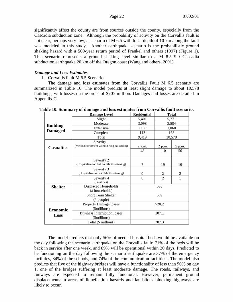
Damage and Loss Estimates1. Corvallis fault M 6.5 Scenario
The damage and loss estimates from the Corvallis Fault M 6.5 scenario aresummarized in Table 10. The model predicts at least slight damage to about 10,578buildings, with losses on the order of $707 million. Damages and losses are detailed inAppendix C.
Table 10. Summary of damage and loss estimates from Corvallis fault scenario.Damage Level Residential Total
Slight 5,401 5,771Moderate 3,098 3,584Extensive 807 1,060Complete 113 163
BuildingDamaged
Total 9,419 10,578
2 a.m. 2 p.m. 5 p.m.Severity 1
(Medical treatment without hospitalization)
48 110 56
Severity 2(Hospitalization but not life threatening) 7 19 10
Severity 3(Hospitalization and life threatening) 0 2 2
Casualties
Severity 4(Fatalities)
0 2 1
Displaced Households(# households)
695Shelter
Short Term Shelter(# people)
659
Property Damage losses($millions)
520.2
Business Interruption losses($millions)
187.1Economic
LossTotal ($ millions) 707.3
The model predicts that only 56% of needed hospital beds would be available onthe day following the scenario earthquake on the Corvallis fault; 71% of the beds will beback in service after one week, and 89% will be operational within 30 days. Predicted tobe functioning on the day following the scenario earthquake are 37% of the emergencyfacilities, 34% of the schools, and 74% of the communication facilities . The model alsopredicts that five of the highway bridges will have a functionality of less than 90% on day1, one of the bridges suffering at least moderate damage. The roads, railways, andrunways are expected to remain fully functional. However, permanent grounddisplacements in areas of liquefaction hazards and landslides blocking highways arelikely to occur.
Page 23 07/02/01
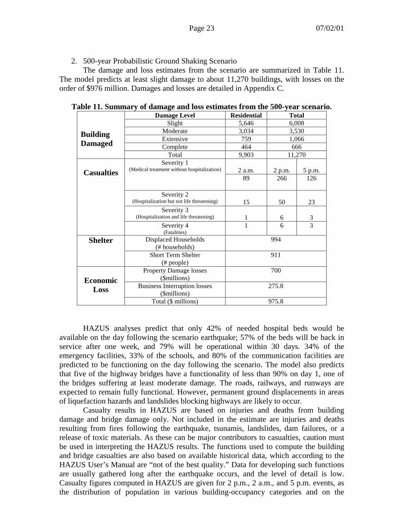
2. 500-year Probabilistic Ground Shaking ScenarioThe damage and loss estimates from the scenario are summarized in Table 11.
The model predicts at least slight damage to about 11,270 buildings, with losses on theorder of $976 million. Damages and losses are detailed in Appendix C.
Table 11. Summary of damage and loss estimates from the 500-year scenario.Damage Level Residential Total
Slight 5,646 6,008Moderate 3,034 3,530Extensive 759 1,066Complete 464 666
BuildingDamaged
Total 9,903 11,270
2 a.m. 2 p.m. 5 p.m.Severity 1
(Medical treatment without hospitalization)
89 266 126
Severity 2(Hospitalization but not life threatening) 15 50 23
Severity 3(Hospitalization and life threatening) 1 6 3
Casualties
Severity 4(Fatalities)
1 6 3
Displaced Households(# households)
994Shelter
Short Term Shelter(# people)
911
Property Damage losses($millions)
700
Business Interruption losses($millions)
275.8Economic
LossTotal ($ millions) 975.8
HAZUS analyses predict that only 42% of needed hospital beds would beavailable on the day following the scenario earthquake; 57% of the beds will be back inservice after one week, and 79% will be operational within 30 days. 34% of theemergency facilities, 33% of the schools, and 80% of the communication facilities arepredicted to be functioning on the day following the scenario. The model also predictsthat five of the highway bridges have a functionality of less than 90% on day 1, one ofthe bridges suffering at least moderate damage. The roads, railways, and runways areexpected to remain fully functional. However, permanent ground displacements in areasof liquefaction hazards and landslides blocking highways are likely to occur.
Casualty results in HAZUS are based on injuries and deaths from buildingdamage and bridge damage only. Not included in the estimate are injuries and deathsresulting from fires following the earthquake, tsunamis, landslides, dam failures, or arelease of toxic materials. As these can be major contributors to casualties, caution mustbe used in interpreting the HAZUS results. The functions used to compute the buildingand bridge casualties are also based on available historical data, which according to theHAZUS User’s Manual are “not of the best quality.” Data for developing such functionsare usually gathered long after the earthquake occurs, and the level of detail is low.Casualty figures computed in HAZUS are given for 2 p.m., 2 a.m., and 5 p.m. events, asthe distribution of population in various building-occupancy categories and on the
Page 24 07/02/01
highways depends on the time of day. Population exposure is computed, and then thecasualty functions are engaged based on percentage of buildings in each of the damagestates.
CONCLUSIONSGreat Cascadia subduction zone earthquakes have occurred many times in the
past along the Pacific Northwest coast, the most recent one on January 26, 1700 (Clagueand others, 2000). Future subduction zone earthquakes pose great seismic hazards andrisk to Benton County. Strong ground shaking from the subduction zone earthquakes willlikely last three minutes or more and be dominated by long-period ground motions(Clague and others, 2000). This long-period and long-duration ground shaking will causewidespread ground failures. The ground shaking hazard from the Cascadia subductionearthquakes and other sources has been assessed and is available in such publications asDOGAMI map GMS-100 (Madin and Mabey, 1996) and the probabilistic hazard maps ofthe United States Geological Survey (USGS) (Frankel and others, 1997). These mapsprovide a general seismic hazard level from all seismic sources. The ground motiondesign level in the State of Oregon 1998 Structural Specialty Code (Oregon BuildingCodes Division, 1998) is based on these probabilistic seismic hazard assessments.
However, the earthquake hazard is also affected by local surface and subsurfacegeologic, hydrologic, and topographic conditions, which allow the differentiation ofrelative earthquake hazards. We assessed these relative hazards in Benton Countyutilizing the best available geological, geotechnical, and water-well data, as well aslimited field investigations. The maps show that the areas with high ground amplificationand liquefaction hazards are concentrated along the Willamette River, while the areaswith high earthquake-induced landslide hazard are spread out over the western part of thecounty in the Coast Range.
Oregon is prone to landslide hazards (Beaulieu, 1976), especially in the westernpart of the state, where steep slopes and conducive geological conditions are combinedwith abundant precipitation (Burns, 1998a). In Benton County, we delineated landslidehazard using a combination of landslide inventory and computer modeling based on thebest available topographic, geologic, and soil data. The results show that Benton Countyhas a low landslide hazard in the eastern part, low to moderate landslide hazard in thenorthwestern part, and moderate to high landslide hazard in the southwestern part of thecounty.
A detailed building survey was conducted for 90 percent of the commercialbuildings in downtown Corvallis. The survey data, along with the available data from theCity of Corvallis, Benton County, and other sources, were analyzed to augment thebuilding inventory provided in HAZUS99. The analysis shows:
(1) Total single-family residential building area from the project data was 22%larger than the HAZUS default data. This is largely due to the fact that certaintracts are growing rapidly, and the survey data are much more up to date thanthe HAZUS default data.
(2) Building quantities for the Oregon State University campus were greatlyunderestimated in the HAZUS default data.
(3) The projected data and HAZUS default data have the same total area forcommercial buildings, although the breakdowns into specific categories arevery different. The projected data show nearly twice as much retail
Page 25 07/02/01
commercial areas and about half as much office space as the HAZUS defaultdata.
(4) Industrial buildings were underestimated by the HAZUS default data, largelydue to the fact that the Hewlett Packard Company, Inc., campus wasunderestimated.
The relative seismic hazard maps, augmented building inventory, and otherinventories provided in HAZUS99 were used to assess seismic risks in the county for twoscenarios: (1) a M 6.5 earthquake on the Corvallis fault and (2) a probabilistic groundmotion with 500-year recurrence interval (Frankel and others, 1997), which is similar tothe ground shaking level generated by a M 8.5�9.0 Cascadia subduction zone earthquake20 km offshore. The results indicate that the damage and losses from the scenarios wouldbe devastating. A M 6.5 earthquake on the Corvallis fault at a depth of 10 km wouldcause at least slight damage to 10,578 buildings, about one hundred injuries and deaths,and approximately $707 million in losses. The 500-year probabilistic ground-shakingscenario would likely cause at least slight damage to 11,270 buildings, more than onehundred injuries and deaths, and approximately $976 million in losses.
DISCUSSIONHazard Maps
The Relative Earthquake Hazard Maps, including ground motion amplification,liquefaction, and earthquake-induced landslide hazards, and the Water-induced LandslideHazard Map for Benton County were developed based on local geologic, topographic,and hydrologic conditions. The local geologic conditions, including thickness andengineering properties of geologic materials, were derived from existing geological,geotechnical, topographic, and water-well data and limited field investigations. Thesedata we used to construct three-dimensional geologic models, using the GIS softwareMapInfo� and Vertical Mapper�. According to the scope of this project, most of thefield investigations were concentrated in the Corvallis area (Corvallis-Philomath urbanarea). Consequently, a better geologic model and landslide inventory for that area wasobtained. Nevertheless, the maps are all at a regional scale, not suitable for site-specificevaluations.
We derived the ground motion amplification hazard from a three-dimensionalgeologic model, using GIS software to assign hazard values on the basis of the UBC-97methodology. Liquefaction hazard was derived in a similar manner, by use of the age anddepositional environment of the geologic units and a simplified state-of-practiceengineering analysis. Earthquake-induced and water-induced landslide hazards wereanalyzed with infinite-slope modeling and with the assumption of the worst hydrologicconditions: 100% saturation or 0 m groundwater table.
The relative earthquake hazard maps and water-induced landslide hazard mapdelineate those areas most likely to experience damage during a strong earthquake orheavy rainfall. This information can be used to develop a variety of hazard mitigationstrategies such as the following:
Emergency response and hazard mitigationOne of the key uses of these maps is to develop emergency response plans. The
areas indicated as having a higher hazard would be the areas where the greatest and mostabundant damage will tend to occur. Planning for disaster response will be enhanced by
Page 26 07/02/01
the use of these maps to identify which resources and transportation routes are likely tobe damaged.
Land use planning The location of future urban expansion or intensified development should also
consider earthquake and landslide hazards. Requirements placed on development couldbe based on the hazard zone in which the development is located. For example, the typeof site-specific hazard investigation that is required for a particular location could bebased on the maps.
LifelinesLifelines include road and access systems such as railroads, airports, and runways,
bridges, and over- and underpasses, as well as utilities and distribution systems. Therelative earthquake and landslide hazard maps are especially useful for estimation andmitigation of expected-damage to lifelines. Lifelines are usually distributed widely andoften require regional as opposed to site-specific hazard assessments. The hazard mapspresented here allow quantitative estimates of the hazard throughout a lifeline system.This information can be used for assessing vulnerability as well as deciding on prioritiesand approaches for mitigation.
EngineeringThe hazard zones shown on the Hazard Maps should not serve as a substitute for
site-specific evaluations based on subsurface information gathered at a site. Thecalculated values of the individual map may, however, be used to good purpose in theabsence of such site-specific information, for instance, at the feasibility-study orpreliminary-design stage. In most cases, the quantitative values calculated for these mapswould be superior to a qualitative estimate based solely on lithology or non-site-specificinformation.
It is very important to recognize the limitations of these hazard maps, which inno way include information with regard to the probability of damage to occur. Rather,they show that when strong ground shaking or heavy rainfall occurs, the damage is morelikely to occur, or be more severe, in the higher hazard areas. However, the higher hazardareas should not necessarily be viewed as unsafe. These limitations result from the natureof regional mapping, data limitations, and computer modeling.
Risk AssessmentHAZUS99 was developed by FEMA and the National Institute of Building
Sciences (NIBS) as a tool for developing reliable earthquake damage and loss estimatesthat are essential to decision-making at the local, regional, state, and national levels ofgovernment. HAZUS99 contains a huge default database, ranging from building stockand lifeline facilities to fragility functions and was developed from available datanationwide. Some default data may not reflect the reality in Benton County. In this study,some effort was made to improve building data by extrapolating the sample buildingsurvey and available information from the City of Corvallis, Benton County, and othersources.
The risk assessment performed in this study can provide the basis for developingmitigation policy, for developing and testing emergency preparedness and response plans,and for planning for postdisaster relief and recovery. However, caution must be exercisedin using the risk information due to the uncertainty and data quality inherent in the
Page 27 07/02/01
HAZUS99 program and associated databases, for example, the uncertainty of earthquakeactivity on Corvallis fault.
ACKNOWLEDGMENTSThis project was supported by a professional services agreement with Benton County
and from resources of the Oregon Department of Geology and Mineral Industries. Countyfunds were derived from the Project Impact program of the Federal EmergencyManagement Agency. Jon Hofmeister of DOGAMI contributed greatly to this project bysharing practical insight on GIS data conversion and manipulation and in-depth review ofthe report. Stephen Dickenson and his students at Oregon State University providedgeotechnical data and shared their soil amplification map in Corvallis area. CarolHasenberg of Portland State University provided many review comments on seismic riskassessment.
REFERENCESAbramson, L.W., T.S. Lee, S. Sharma, and G.M. Boyce, 1996, Stability and Stabilization
Methods, John Wiley & Sons, Inc, New York.Allison, I.S., 1953, Geology of the Albany Quadrangle, Oregon: Oregon Department of
Geology and Mineral Industries Bulletin 37, 18 p.Andrus, R.D., and Stokoe, K.H., 1997, Liquefaction resistance based on shear wave
velocity: Report to the NCEER Workshop on Evaluation of Liquefaction Resistance (9/18/97 version), Jan. 4-5, Salt Lake City, Utah.
Atwater, B.F., 1987, Evidence for great Holocene earthquakes along the outer coast of Washington state: Science, v. 236, p. 942-944.
Atwater, B.F., and Hemphill-Haley, E., 1997, Recurrence intervals for great earthquakes of the past 3,500 years at northeastern Willapa Bay, Washington: U.S. GeologicalSurvey Professional Paper 1576, 108 p.
Baldwin, E.M., 1955, Geology of the Marys Peak and Alsea Quadrangles, Oregon: U.S. Geological Survey Oil and Gas Investigations Map OM-162, scale: 1:62500.
Beaulieu, J.D., 1973, Environmental geology of inland Tillamook and Clatsop Counties,Oregon: Oregon Department of Geology and Mineral Industries Bulletin 79, 65p., map scale 1:62,500.
Beaulieu, J.D., 1976, Geologic Hazards in Oregon, Ore Bin, v. 38, no. 5, p 67-86.Bela, J.L., 1979, Geologic Hazards of eastern Benton County, Oregon: Oregon
Department of Geology and Mineral Industries Bulletin 98, 122 p.Black, G.L., Wang, Z., Wiley, T.J., Wang, Y., and Keefer, D.K., 2000a, Relative
earthquake hazards of the Eugene-Springfield metropolitan area, Lane County,Oregon: Oregon Department of Geology and Mineral Industries Interpretive MapSeries IMS-14, 1:24,000.
Black, G.L., Wang, Z., and Priest, G.R., 2000b, Relative earthquake hazard map of the Klamath Falls metropolitan area, Klamath County, Oregon: Oregon Department of Geology and Mineral Industries Interpretive Map Series IMS-19, 1:24,000.
Bolt, B.A., 1993, Earthquakes: New York, W.H. Free man and Co., 331 p.Building Seismic Safety Council, 1994, NEHERP recommended provisions for seismic
regulations for new buildings, 1994 edition, Part 1: Provisions: FederalEmergency Management Agency Publication FEMA 222A / May 1995, 290 p.
Burns, S. F., 1998a, Landslide Hazards in Oregon, Environmental, Groundwater and
Page 28 07/02/01
Engineering Geology, ed. By S. Burns, Star Publishing Company, Belmont, CA,p303-315.
Burns, S. F., 1998b, Landslides in the Portland Area resulting from the Storm of February, 1996, Environmental, Groundwater and, Engineering Geology, ed. By S. Burns, Star Publishing Company, Belmont, CA, p353-365.
Clague, J.J., Atwater, B.F., Wang, K., Wang, Y., and Wong, I., 2000, Program Summary and Abstracts, Penrose Conference 2000: Oregon Department of Geology and Mineral Industries Special Paper 33.
Corliss, J.F., 1973, Soil survey of Alsea area, Oregon: U.S. Department of Agriculture, Soil Conservation Service, 82 p.
Driscoll, D.D., 1979, Retaining wall design guide: Portland, Oregon, U.S. Department ofAgriculture, Forest Service, Pacific Northwest Region.
Frankel, A., Mueller, C., Barnhard, T., Perkins, D., Leyendecker, E. V., Dickman, N.,Hanson, S., and Hopper, M., 1997, National 1996 Seismic Hazard Maps: U.S.Geological Survey, Open-File Report 97-131.
Geomatrix Consultants, Inc., 1995, Seismic design mapping, State of Oregon: Final report to Oregon Department of Transportation, Project no. 2442, var. pag.
Goldfinger, C., 1990, Evolution of the Corvallis Fault and Implications for the Oregon Coast Range, MS Thesis, Oregon State University, Corvallis, Oregon, 118p.
Harvey, A.F. and G.L. Peterson, 1998, Water-Induced Landslide Hazards: Western Portion of the Salem Hills, Marion County, Oregon, Oregon Department ofGeology and Mineral Industries Interpretive Map Series IMS-6.
Harvey, A.F. and G.L. Peterson, 2000, Water-Induced Landslide Hazards: Eastern Portion of the Eola Hills, Polk County, Oregon, Oregon Department of Geologyand Mineral Industries Interpretive Map Series IMS-5.
Heaton, T.H., and Hartzell, S.H., 1987, Earthquake hazards on the Cascadia subductionzone: Science, v. 236, p. 162–168.
Hofmeister, R.J., 2000, Slope failures in Oregon: GIS inventory for three 1996/97 storm events: Oregon Department of Geology and Mineral Industries Special Paper 34, 20 p.
Hofmeister, R.J., Wang Y., Keefer D.K., 2000a, Earthquake-Induced Slope Instability: Relative Hazard Map Western Portion of the Salem Hills, Marion County,Oregon, Oregon Department of Geology and Mineral Industries Interpretive MapSeries IMS-17.
Hofmeister, R.J., and Wang Y., 2000, Earthquake-Induced Slope Instability: Relative Hazard Map Western Portion of the Salem Hills, Marion County, Oregon, OregonDepartment of Geology and Mineral Industries Interpretive Map Series IMS-18.
Hofmeister R.J., Wang, Y., and Keefer, D.K., 2000b, Earthquake-induced slope instability: methodology of relative hazard mapping, western portion of the SalemHills, Marion County, Oregon: Oregon Department of Geology and MineralIndustries Special Paper 30, 73 p.
Holzer, T.H., 1994, Loma Prieta damage largely attributed to enhanced ground shaking:EOS, v. 75, no. 26, p. 299-301 [reprinted in Oregon Geology, v. 56, no. 5 (Sept. 1994, p. 111-113].
International Conference of Building Officials, 1997, 1997 Uniform building code, v. 2, Structural design provisions: International Conference of Building Officials, 492 p.
Jibson, R.W., 1993, Predicting earthquake-induced landslide deposits using Newmark’s sliding block analysis: Washington, D.C., National Research Council
Page 29 07/02/01
Transportation Research Record 1411, p. 9-17. Jibson, R.W., 1996, Use of landslides for paleoseismic analysis: Engineering Geology,
v. 43, p. 291-323.Jibson, R.W., Harp, E.L., and Michael, J.A., 1998, A method for producing digital
probabilistic seismic landslide hazard maps: an example from the Los Angeles, California, area: U.S. Geological Survey Open-file Report 98-113.
Jibson, R.W., and Keefer, D.K., 1993, Analysis of the seismic origin of landslides: Examples from the New Madrid seismic zone: Geological Society of AmericaBulletin, v. 105, p. 521-536.
Keefer, D.K., 1984, Landslides caused by earthquakes: Geological Society of AmericaBulletin, v. 95, p. 406-421.
Keefer, D.K., 1993, The susceptibility of rock slopes to earth-quake induced failure: Association of Engineering Geologists Bulletin, v. 30, p. 353-361.
Keefer, D.K., and Schuster, R.L., 1993, A method for predicting slope instability forearthquake hazard maps, preliminary report: Association of Engineering Geologists Special Publication 10, p. 39-52.
Knezevich, C.A., 1975, Soil survey of Benton County area, Oregon: U.S. Department of Agriculture, Soil Conservation Service, 119 p.
Langridge, R.W., 1987, Soil survey of the Linn County area, Oregon: U.S. Department of Agriculture, Soil Conservation Service, 344 p.
Mabey, M.A., Madin, I.P., and Meier, D.B., 1995a, Relative earthquake hazard map of the Beaverton quadrangle, Washington County, Oregon: Oregon Department ofGeology and Mineral Industries Geologic Map Series GMS-90.
Mabey, M.A., Madin, I.P., and Meier, D.B., 1995b, Relative earthquake hazard map of the Lake Oswego quadrangle, Clackamas, Multnomah, and Washington Counties,
Oregon: Oregon Department of Geology and Mineral Industries Geologic Map Series GMS-91.
Mabey, M.A., Madin, I.P., and Meier, D.B., 1995c, Relative earthquake hazard map of the Gladstone quadrangle, Clackamas and Multnomah Counties, Oregon: Oregon Department of Geology and Mineral Industries Geologic Map Series GMS-92.
Mabey, M.A., Madin, I.P., Meier, D.B., and Palmer, S.P., 1995d, Relative earthquake hazard map of the Mount Tabor quadrangle, Multnomah County, Oregon: OregonDepartment of Geology and Min eral Industries Geological Map Series GMS–89.
Madin, I.P., Priest, G.R., Mabey, M.A., Malone, S., Yelin, T.S., Meier, D., 1993, March23, 1993, Scotts Mills earthquake-western Oregon’s wake-up call: OregonGeology, v. 55, no. 3, p. 51-57.
Madin, I.P., and Mabey, M.A., 1996, Earthquake hazard maps for Oregon: Oregon Department of Geology and Mineral Industries Geologic Map Series GMS-100.
Madin, I.P., and Wang, Z., 1999a, Relative earthquake hazard maps for selected urban areas in western Oregon: Astoria-Warrentown, Brookings, Coquille, Florence-Dunes City, Lincoln City, Newport, Reedsport-Winchester Bay, Seaside-Gearhart-Cannon Beach, Tillamook: Oregon Department of Geology and MineralIndustries Interpretive Map Series IMS-10.
Madin, I.P., and Wang, Z., 1999b, Relative earthquake hazard maps for selected urban areas in western Oregon: Ashland, Cottage Grove, Grants Pass, Roseburg, Sutherlin-Oakland: Oregon Department of Geology and Mineral IndustriesInterpretive Map Series IMS-9.
Madin, I.P., and Wang, Z., 1999c, Relative earthquake hazard maps for selected urban
Page 30 07/02/01
areas in western Oregon: Canby-Barlow-Aurora, Lebanon, Silverton-Mount Angel, Stayton-Sublimity-Aumsville, Sweet Home, Woodburn-Hubbard: Oregon Department of Geology and Mineral Industries Interpretive Map Series IMS-8.
Madin, I.P., and Wang, Z., 1999d, Relative earthquake hazard maps for selected urban areas in western Oregon: Dallas, Hood River, McMinnville-Dayton-LaFayette, Monmouth-Independence, Newberg-Dundee, Sandy, Sheridan-Willamina,St. Helens-Columbia City-Scappoose: Oregon Department of Geology and Mineral Industries Interpretive Map Series IMS-7.
McCrink, T.P., and Real, C.R., 1996, Evaluation of the Newmark method for mapping earthquake-induced landslide hazards in the Laurel 7.5’ quadrangle, Santa Cruz County, California: Final Technical Report, California Department Conservation,Division of Mines and Geology.
National Institute of Building Sciences (NIBS), 1997, HAZUS, earthquake loss estimation methodology, prepared for the Federal Emergency ManagementAgency (FEMA): NIBS Documents 5200 (user's manual) and 5201-5203(technical manual, 3 vols.). var. pag.
National Institute of Building Sciences (NIBS), 1999, HAZUS, FEMA's tool for estimating potential losses from natural disasters: Available on CD-ROM disksfrom National Institute of Building Sciences 1090 Vermont Avenue, NW, Suite700 Washington, DC, 20005-4905, phone (202) 289-7800, fax (202) 289-1092, e-mail [email protected]. Internet http://www .fema.gov/HAZUS/
National Research Council, Commission on Engineering and Technical Systems, Committee on Earthquake Engineering, 1985, Liquefaction of soils duringEarthquakes: Washington, D.C., National Academy Press, 240 p.
National Research Council, Transportation Research Board, 1996, Landslides Investigation and Mitigation, Special Report 247, ed. By K. Turner and R.L.Schuster, p673.
Naval Facilities Engineering Command (NFEC), 1986, Soil mechanics: Naval FacilitiesEngineering Command Design Manual 7.01, 348 p.
Newmark, N.M., 1965, Effects of earthquakes on dams and embankments: Geotechnique, v. 15, p. 139-159.
O’Connor, J.E., Sarna-Wojcicki, A.M., Wozniak, K.C., Polette, D.J., and Fleck, R.J., 2000, Origin, extent, and thickness of Quaternary geologic units in the Willamette Valley, Oregon: U.S. Geological Survey Professional Paper 1620, 52 p.
Patching, W.R., 1987, Soil survey of Lane County area, Oregon: U.S. Department ofAgriculture, Soil Conservation Service, 369 p.
Rad, F.N. Rad, C.S. Hasenberg, 2000, Building Inventory Analysis for Benton County,Oregon, Department of Civil Engineering, Portland State University, 23p.
Schlicker, H.G., Deacon, R.J., Beaulieu, J.D., and Olcott, G.W., 1972, Environmentalgeology of the coastal region of Tillamook and Clatsop Counties, Oregon: OregonDepartment of Geology and Mineral Industries Bulletin 74, 164 p.
Seed, H.B., and Idriss, I.M., 1971, Simplified Procedure for Evaluation Soil Liquefaction Potential, Journal of the Soil Mechanics and Foundation Division, ASCE, Vol. 97,SM9, p1249-1273.
Seed, H.B., and Idriss, I.M., 1982, Ground motions and soil liquefaction during earthquakes: Earthquake Engineering Institute Monograph Series, 134 p.
Seed, H.B., Romo, M.P., Sun, J.I., Jaime, A., and Lysmer, J., 1988, The Mexicoearthquake of September 19,1985-relationship between soil conditions and
Page 31 07/02/01
earthquake ground motions: Earthquake Spectra, v. 4, p. 687-729.U.S. Department of Agriculture (USDA), 1981, Transportation engineering handbook,
Region 1, supplement 11: Missoula, Montana, U.S. Department of Agriculture,Forest Service, Northern Region.
U.S. Department of Agriculture (USDA), 1996, Soil survey laboratory manual: USDA Natural Resources Conservation Service Soil Survey Investigations Report 42,version 3.0, 693 p.
U.S. Department of Agriculture (USDA), 1994, Slope stability reference guide fornational forests in the United States, volume I: Washington, D.C., USDA Forest Service Engineering Staff Report EM-7170-13.
Vokes, H.E., Myers, D.A., and Hoover, L., 1954, Geology of the west-central border area
of the Willamette Valley, Oregon: U.S. Geological Survey Oil and GasInvestigations Map OM-150, scale: 1:62500.
Walker, G.W., and Duncan, R.A., 1989, Geologic map of the Salem 1� by 2� quadrangle,western Oregon: U.S. Geological Survey Miscellaneous Investigations Series Map I-1893, scale 1:250000.
Walker, G.W., and MacLeod, N.S., 1991, Geologic map of Oregon: U.S. Geological Survey, scale 1:500000.
Wang, Y. and Leonard, W.J., 1996, Relative earthquake hazard maps of the Salem East and Salem West quadrangles, Marion and Polk Counties, Oregon: Oregon Department of Geology and Mineral Industries Geologic Map Series GMS-105.
Wang, Y. and J.L. Clark, 1999, Earthquake Damage in Oregon: Preliminary Estimates of Future Earthquake Losses, Special Paper 29, Oregon Department of Geology andMineral Industries, p59.
Wang, Z., Madin, I.P., and Street, R.L., 1998, Shear-wave velocity and soil classifications for communities in Oregon: Proceedings of the 8th International IAEG Congress, Vancouver, British Columbia, Canada, September 21-25, 1998, p. 149-154.
Wang, Z., R. L. Street, E. W. Woolery, and I. P. Madin, 2000, SH-WaveRefraction/Reflection and Site Characterization, Use of Geophysical Methods inConstruction (Getechnical Special Publication No. 108), Proceedings of Sectionsof GEO-Denver 2000, ed. By S. Nazarian and J. Diehl, ASCE, Reston, Virginia,p. 126-140.
Wang, Z., and Wang, Y., 2000, Earthquake hazard maps and seismic risk assessment for Klamath County, Oregon: Oregon Department of Geology and Mineral Industries Interpretive Map Series IMS-20, 28 p.
Wang, Z., C.S. Hasenberg, G.B. Graham, and F.N. Rad, 2001, Seismic Hazard and Risk Assessments in Tillamook County, Oregon, Oregon Department of Geology andMineral Industries (in press).
Weaver, C.S., and Shedlock, K.M., 1989, Potential subduction, probable intraplate, and known crustal earthquake source areas in the Cascadia subduction zone, in Hays,W.W., ed., 3rd Annual Workshop on “Earthquake Hazards in the Puget Sound,Portland Area,” Proceedings: U.S. Geological Survey Open-File Report 89–465,p. 11–26.
Weiczorek, G.F., Wilson, R.C., and Harp, E.L., 1985, Map showing slope stability during
earthquakes in San Mateo County, California: U.S. Geological Survey Miscellaneous Investigations Series Map I-1257-E, scale 1:62,500.
Page 32 07/02/01
Wiley, T.J., Sherrod, D.R., Keefer, D.K., Qamar, A., Schuster, R.L., Dewey, J.W.,Mabey, M.A., Black, G.L., and Wells, R.E., 1993, Klamath Falls Earthquake,September 20, 1993-Including the strongest quake ever measured in Oregon,Oregon Geology, v. 55, p. 127-134.
Yeats, R.S., Graven, E.P., Werner, K.S., Goldfinger, C., and Popowski, T.S, 1991, Tectonics of the Willamette Valley, Oregon, in Rogers, A.M., Walsh, T.J.,Kockelman, W.J., and Priest, G.R., eds., Assessing earthquake hazards and reducing risk in the Pacific Northwest, volume 1: U.S. Geological Survey Professional Paper 1560, p. 183-222.
Yelin, T.S., Tarr, A.C., Michael, J.A., and Weaver, C.S., 1994, Washington and Oregon Earthquake history hazards: U.S. Geological Survey Open File Report 94-226-B,11 p.
Youd, T.L. and D.M. Perkins, 1978, Mapping Liquefaction-Induced Ground Failure Potential, Journal of the Geotechnical Engineering Division, ASCE, Vol. 104, No.GT4, p433-446.

Page 33 07/02/01
Appendix A. SH-wave Velocity Data

Page 34 07/02/01
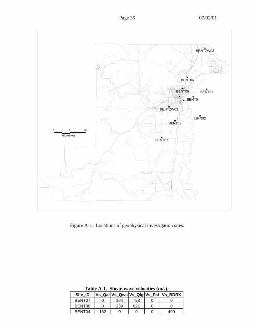
Page 35 07/02/01
0 5
kilometers
10
BENT07
BENT08
BENT04
BENT06
BENT05 BENT01
LINN02
BENTZW02
BENTZW03
Figure A-1. Locations of geophysical investigation sites.
Table A-1. Shear-wave velocities (m/s). Site_ID Vs_Qal Vs_Qws Vs_Qlg Vs_Pal Vs_BDRXBENT07 0 164 723 0 0BENT08 0 239 621 0 0BENT04 162 0 0 0 490
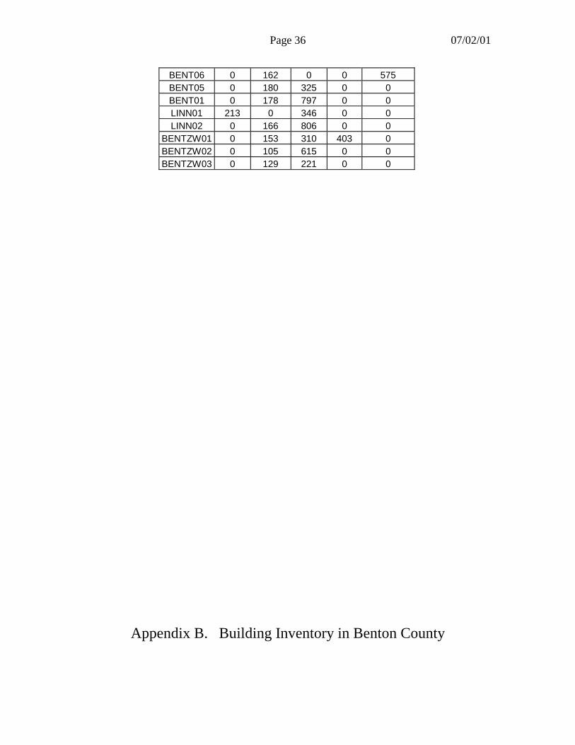
Page 36 07/02/01
BENT06 0 162 0 0 575BENT05 0 180 325 0 0BENT01 0 178 797 0 0LINN01 213 0 346 0 0LINN02 0 166 806 0 0
BENTZW01 0 153 310 403 0BENTZW02 0 105 615 0 0BENTZW03 0 129 221 0 0
Appendix B. Building Inventory in Benton County

Page 37 07/02/01
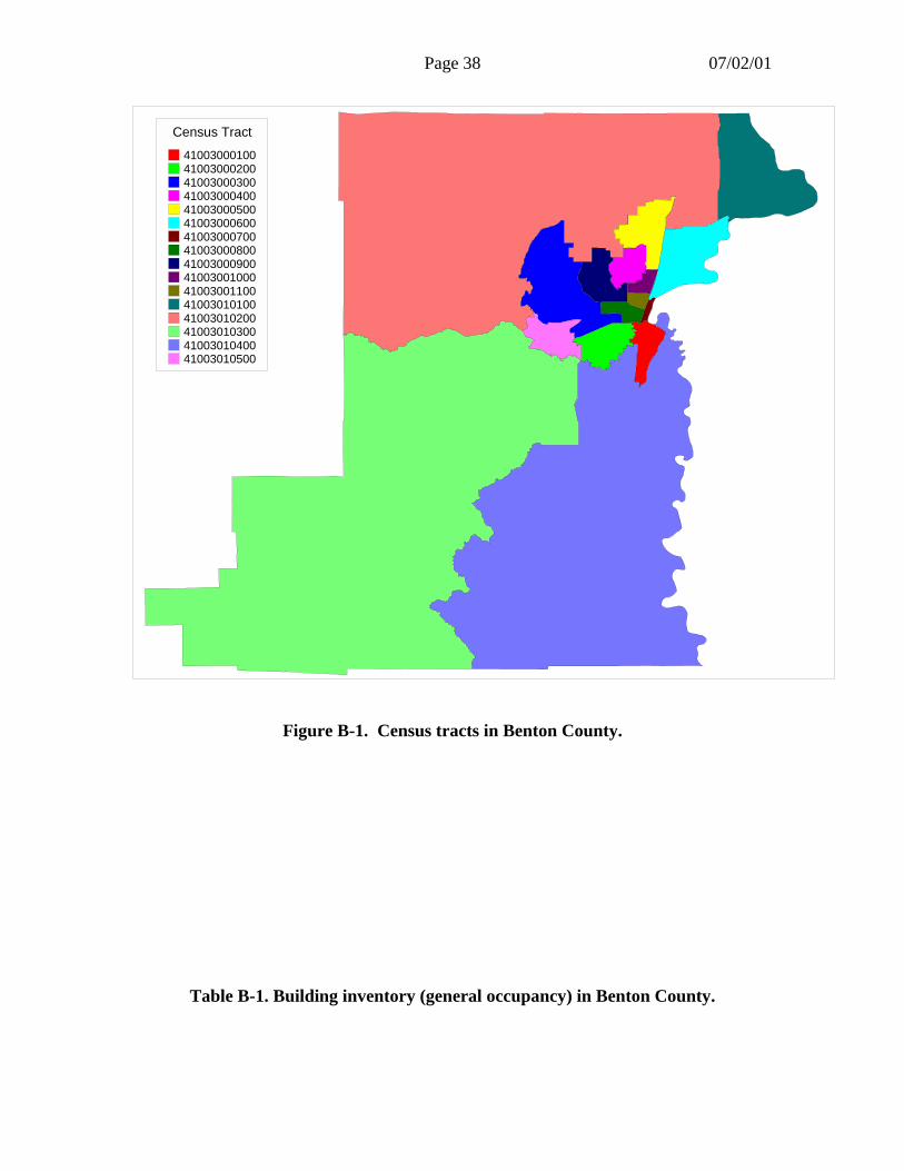
Page 38 07/02/01
Census Tract
41003000100410030002004100300030041003000400410030005004100300060041003000700410030008004100300090041003001000410030011004100301010041003010200410030103004100301040041003010500
Figure B-1. Census tracts in Benton County.
Table B-1. Building inventory (general occupancy) in Benton County.
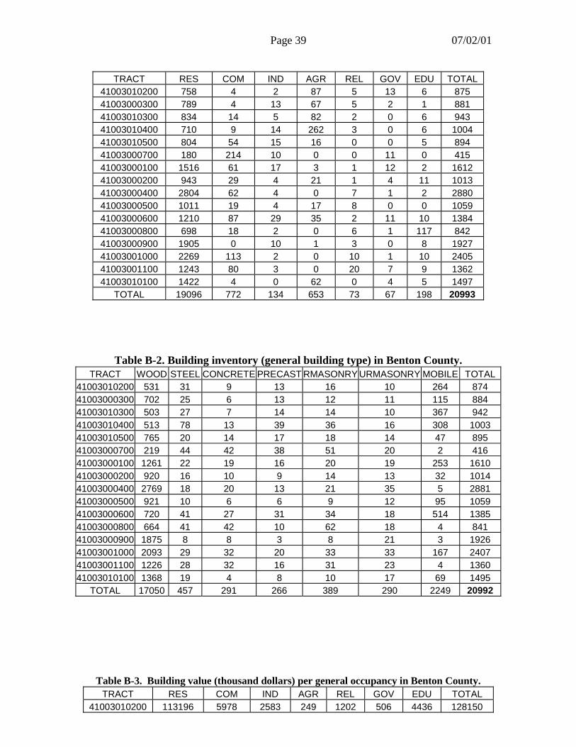
Page 39 07/02/01
Table B-2. Building inventory (general building type) in Benton County.TRACT WOOD STEEL CONCRETE PRECAST RMASONRY URMASONRY MOBILE TOTAL
41003010200 531 31 9 13 16 10 264 87441003000300 702 25 6 13 12 11 115 88441003010300 503 27 7 14 14 10 367 94241003010400 513 78 13 39 36 16 308 100341003010500 765 20 14 17 18 14 47 89541003000700 219 44 42 38 51 20 2 41641003000100 1261 22 19 16 20 19 253 161041003000200 920 16 10 9 14 13 32 101441003000400 2769 18 20 13 21 35 5 288141003000500 921 10 6 6 9 12 95 105941003000600 720 41 27 31 34 18 514 138541003000800 664 41 42 10 62 18 4 84141003000900 1875 8 8 3 8 21 3 192641003001000 2093 29 32 20 33 33 167 240741003001100 1226 28 32 16 31 23 4 136041003010100 1368 19 4 8 10 17 69 1495
TOTAL 17050 457 291 266 389 290 2249 20992
Table B-3. Building value (thousand dollars) per general occupancy in Benton County.TRACT RES COM IND AGR REL GOV EDU TOTAL
41003010200 113196 5978 2583 249 1202 506 4436 128150
TRACT RES COM IND AGR REL GOV EDU TOTAL41003010200 758 4 2 87 5 13 6 87541003000300 789 4 13 67 5 2 1 88141003010300 834 14 5 82 2 0 6 94341003010400 710 9 14 262 3 0 6 100441003010500 804 54 15 16 0 0 5 89441003000700 180 214 10 0 0 11 0 41541003000100 1516 61 17 3 1 12 2 161241003000200 943 29 4 21 1 4 11 101341003000400 2804 62 4 0 7 1 2 288041003000500 1011 19 4 17 8 0 0 105941003000600 1210 87 29 35 2 11 10 138441003000800 698 18 2 0 6 1 117 84241003000900 1905 0 10 1 3 0 8 192741003001000 2269 113 2 0 10 1 10 240541003001100 1243 80 3 0 20 7 9 136241003010100 1422 4 0 62 0 4 5 1497
TOTAL 19096 772 134 653 73 67 198 20993
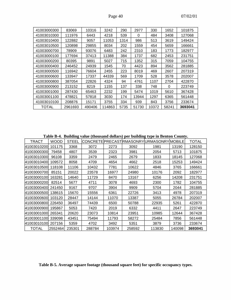
Page 40 07/02/01
41003000300 83069 10316 3242 290 2977 330 1652 10187541003010300 111976 6443 4218 539 0 484 3408 12706841003010400 122882 9057 11053 1314 986 513 3619 14942441003010500 120898 29855 8034 202 1559 454 5659 16666141003000700 78909 93076 6483 242 2310 183 1773 18297741003000100 177694 37413 11388 384 1737 682 2453 23175141003000200 80395 9891 5027 715 1352 315 7059 10475541003000400 246452 24939 1545 70 4423 894 3562 28188541003000500 116942 76604 2455 223 8019 469 2607 20731941003000600 133947 17337 44339 569 1709 528 3578 20200741003000800 387054 22826 4324 94 4761 1107 2704 42287041003000900 213152 8219 1155 137 338 748 0 22374941003001000 287430 65463 2232 199 5474 1019 5610 36742841003001100 478821 57818 3030 174 13944 1297 6365 56144841003010100 208876 15171 3755 334 939 843 3756 233674
TOTAL 2961693 490406 114863 5735 51730 10372 58241 3693041
Table B-4. Building value (thousand dollars) per building type in Benton County.TRACT WOOD STEEL CONCRETE PRECAST RMASONRY URMASONRY MOBILE TOTAL
41003010200 101175 3368 3072 2273 3092 1981 13190 12815041003000300 79458 4807 3539 2323 3981 2054 5713 10187541003010300 96108 3359 2479 2465 2679 1833 18145 12706841003010400 109572 8058 4709 4654 4662 2518 15253 14942441003010500 118108 11106 10432 7781 10622 4846 3765 16666141003000700 85151 20022 23578 16977 24980 10176 2092 18297741003000100 163281 14640 11729 8470 13167 6256 14208 23175141003000200 82514 5677 4711 3078 4693 2300 1782 10475541003000400 241450 9167 9707 3904 9909 5704 2044 28188541003000500 138615 15670 15556 6361 22726 3413 4978 20731941003000600 103120 28447 14144 11070 13387 5055 26784 20200741003000800 226450 36497 74439 6500 50788 22935 5261 42287041003000900 195867 5053 7420 2019 6332 4411 2647 22374941003001000 265341 20620 23073 10814 23951 10985 12644 36742841003001100 339098 43451 75494 11793 58272 25484 7856 56144841003010100 207156 5359 4702 3492 5351 3879 3736 233674
TOTAL 2552464 235301 288784 103974 258592 113830 140098 3693041
Table B-5. Average square footage (thousand square feet) for specific occupancy types.
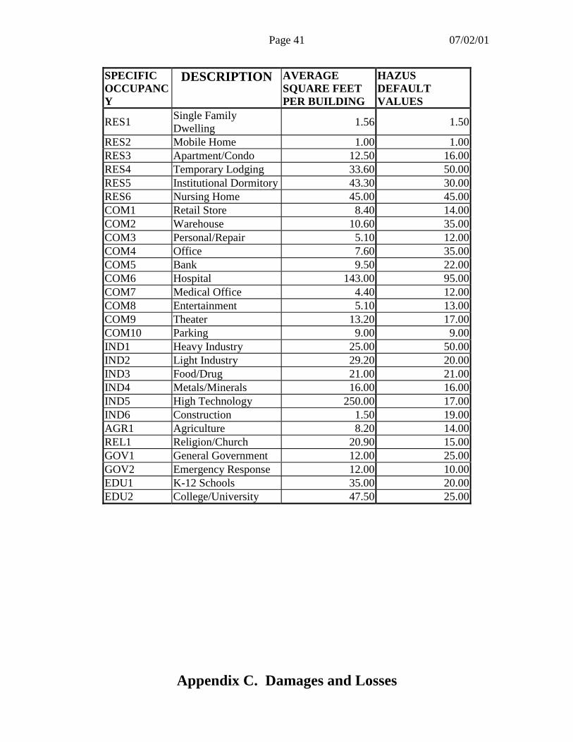
Page 41 07/02/01
SPECIFICOCCUPANCY
DESCRIPTION AVERAGESQUARE FEETPER BUILDING
HAZUSDEFAULTVALUES
RES1 Single FamilyDwelling 1.56 1.50
RES2 Mobile Home 1.00 1.00RES3 Apartment/Condo 12.50 16.00RES4 Temporary Lodging 33.60 50.00RES5 Institutional Dormitory 43.30 30.00RES6 Nursing Home 45.00 45.00COM1 Retail Store 8.40 14.00COM2 Warehouse 10.60 35.00COM3 Personal/Repair 5.10 12.00COM4 Office 7.60 35.00COM5 Bank 9.50 22.00COM6 Hospital 143.00 95.00COM7 Medical Office 4.40 12.00COM8 Entertainment 5.10 13.00COM9 Theater 13.20 17.00COM10 Parking 9.00 9.00IND1 Heavy Industry 25.00 50.00IND2 Light Industry 29.20 20.00IND3 Food/Drug 21.00 21.00IND4 Metals/Minerals 16.00 16.00IND5 High Technology 250.00 17.00IND6 Construction 1.50 19.00AGR1 Agriculture 8.20 14.00REL1 Religion/Church 20.90 15.00GOV1 General Government 12.00 25.00GOV2 Emergency Response 12.00 10.00EDU1 K-12 Schools 35.00 20.00EDU2 College/University 47.50 25.00
Appendix C. Damages and Losses

Page 42 07/02/01
C-1. Damages and Losses From the M 6.5 Corvallis Fault Scenario
Table C-1-1. Expected building damage by general occupancy.TRACT OCCU NONE SLIGHTMODERATE EXTENSIVCOMPLETE41003010200RES 442 179 113 22 3
COM 3 0 0 0 0IND 1 1 0 0 0AGR 53 17 14 3 0REL 3 1 1 0 0GOV 9 3 1 0 0EDU 3 1 1 0 0TOTAL 514 202 130 25 3
41003000300RES 508 186 82 15 1COM 3 0 0 0 0IND 8 3 2 0 0AGR 40 14 11 3 0REL 3 1 1 0 0GOV 2 0 0 0 0EDU 1 0 0 0 0TOTAL 565 204 96 18 1
41003010300RES 468 210 137 21 0COM 9 1 1 0 0IND 4 1 1 0 0AGR 50 17 12 3 0REL 1 0 0 0 0GOV 0 0 0 0 0EDU 4 1 1 0 0TOTAL 536 230 152 24 0
41003010400RES 273 197 176 59 7COM 3 1 2 1 0IND 4 3 4 3 0AGR 101 61 65 30 5REL 1 1 1 0 0GOV 0 0 0 0 0EDU 2 1 1 1 0TOTAL 384 264 249 94 12
41003010500RES 537 186 70 13 1COM 34 8 8 3 0IND 8 3 3 1 0AGR 9 3 2 1 0REL 0 0 0 0 0GOV 0 0 0 0 0EDU 3 1 1 0 0TOTAL 591 201 84 18 1
41003000700RES 66 61 40 9 0COM 45 41 71 46 15
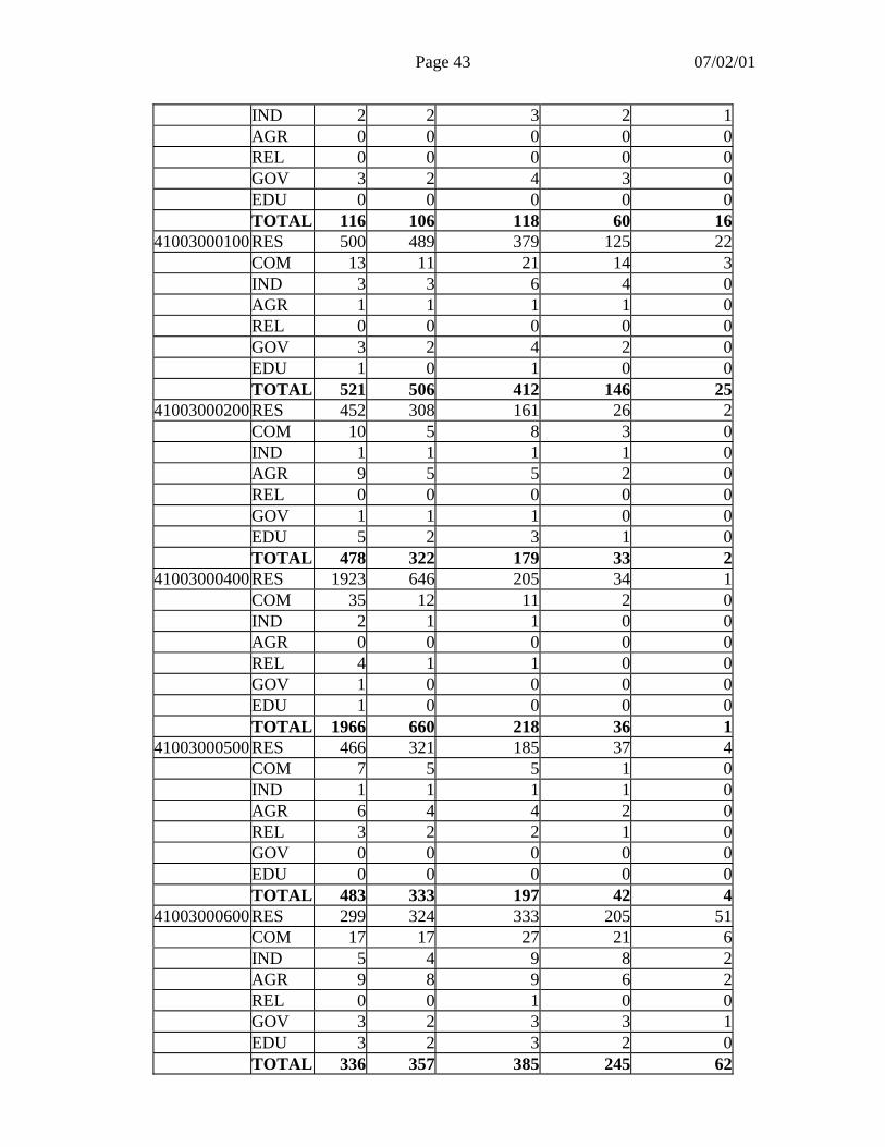
Page 43 07/02/01
IND 2 2 3 2 1AGR 0 0 0 0 0REL 0 0 0 0 0GOV 3 2 4 3 0EDU 0 0 0 0 0TOTAL 116 106 118 60 16
41003000100RES 500 489 379 125 22COM 13 11 21 14 3IND 3 3 6 4 0AGR 1 1 1 1 0REL 0 0 0 0 0GOV 3 2 4 2 0EDU 1 0 1 0 0TOTAL 521 506 412 146 25
41003000200RES 452 308 161 26 2COM 10 5 8 3 0IND 1 1 1 1 0AGR 9 5 5 2 0REL 0 0 0 0 0GOV 1 1 1 0 0EDU 5 2 3 1 0TOTAL 478 322 179 33 2
41003000400RES 1923 646 205 34 1COM 35 12 11 2 0IND 2 1 1 0 0AGR 0 0 0 0 0REL 4 1 1 0 0GOV 1 0 0 0 0EDU 1 0 0 0 0TOTAL 1966 660 218 36 1
41003000500RES 466 321 185 37 4COM 7 5 5 1 0IND 1 1 1 1 0AGR 6 4 4 2 0REL 3 2 2 1 0GOV 0 0 0 0 0EDU 0 0 0 0 0TOTAL 483 333 197 42 4
41003000600RES 299 324 333 205 51COM 17 17 27 21 6IND 5 4 9 8 2AGR 9 8 9 6 2REL 0 0 1 0 0GOV 3 2 3 3 1EDU 3 2 3 2 0TOTAL 336 357 385 245 62
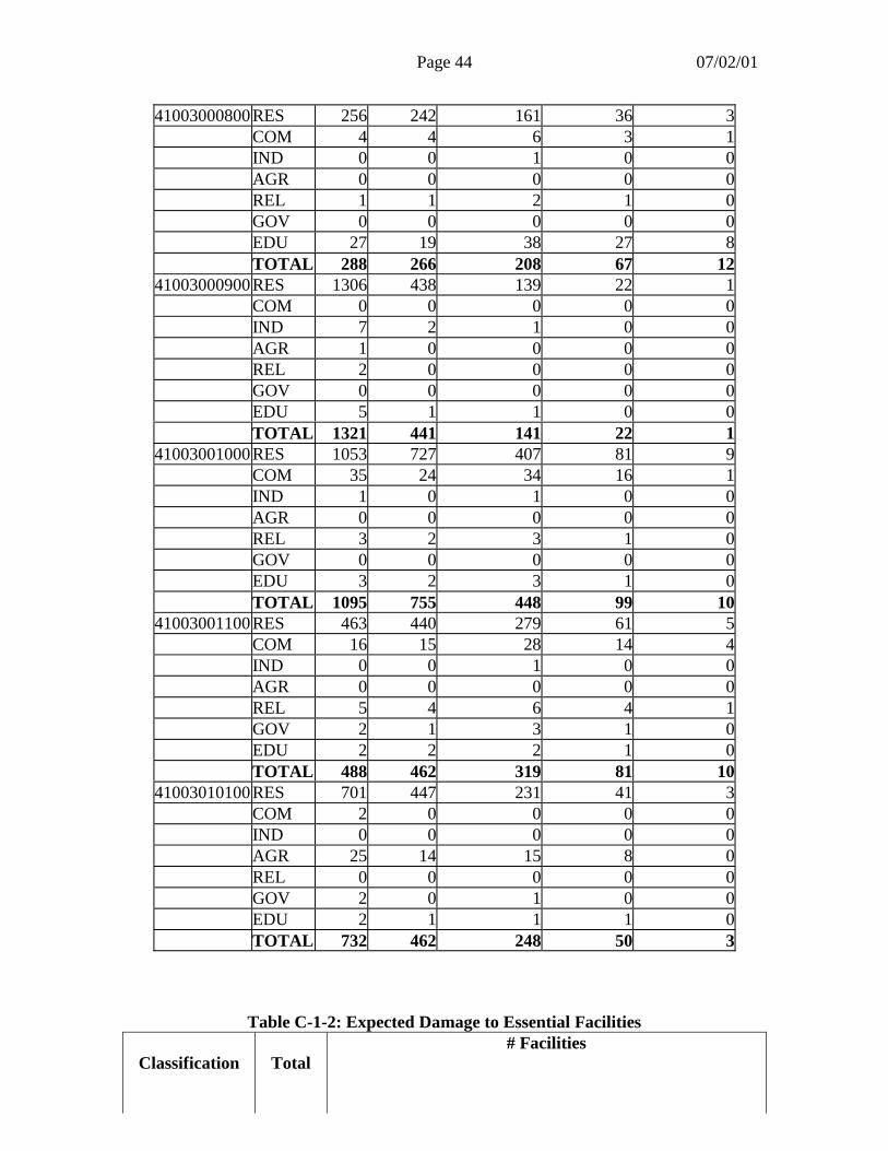
Page 44 07/02/01
41003000800RES 256 242 161 36 3COM 4 4 6 3 1IND 0 0 1 0 0AGR 0 0 0 0 0REL 1 1 2 1 0GOV 0 0 0 0 0EDU 27 19 38 27 8TOTAL 288 266 208 67 12
41003000900RES 1306 438 139 22 1COM 0 0 0 0 0IND 7 2 1 0 0AGR 1 0 0 0 0REL 2 0 0 0 0GOV 0 0 0 0 0EDU 5 1 1 0 0TOTAL 1321 441 141 22 1
41003001000RES 1053 727 407 81 9COM 35 24 34 16 1IND 1 0 1 0 0AGR 0 0 0 0 0REL 3 2 3 1 0GOV 0 0 0 0 0EDU 3 2 3 1 0TOTAL 1095 755 448 99 10
41003001100RES 463 440 279 61 5COM 16 15 28 14 4IND 0 0 1 0 0AGR 0 0 0 0 0REL 5 4 6 4 1GOV 2 1 3 1 0EDU 2 2 2 1 0TOTAL 488 462 319 81 10
41003010100RES 701 447 231 41 3COM 2 0 0 0 0IND 0 0 0 0 0AGR 25 14 15 8 0REL 0 0 0 0 0GOV 2 0 1 0 0EDU 2 1 1 1 0TOTAL 732 462 248 50 3
Table C-1-2: Expected Damage to Essential Facilities
Classification Total# Facilities
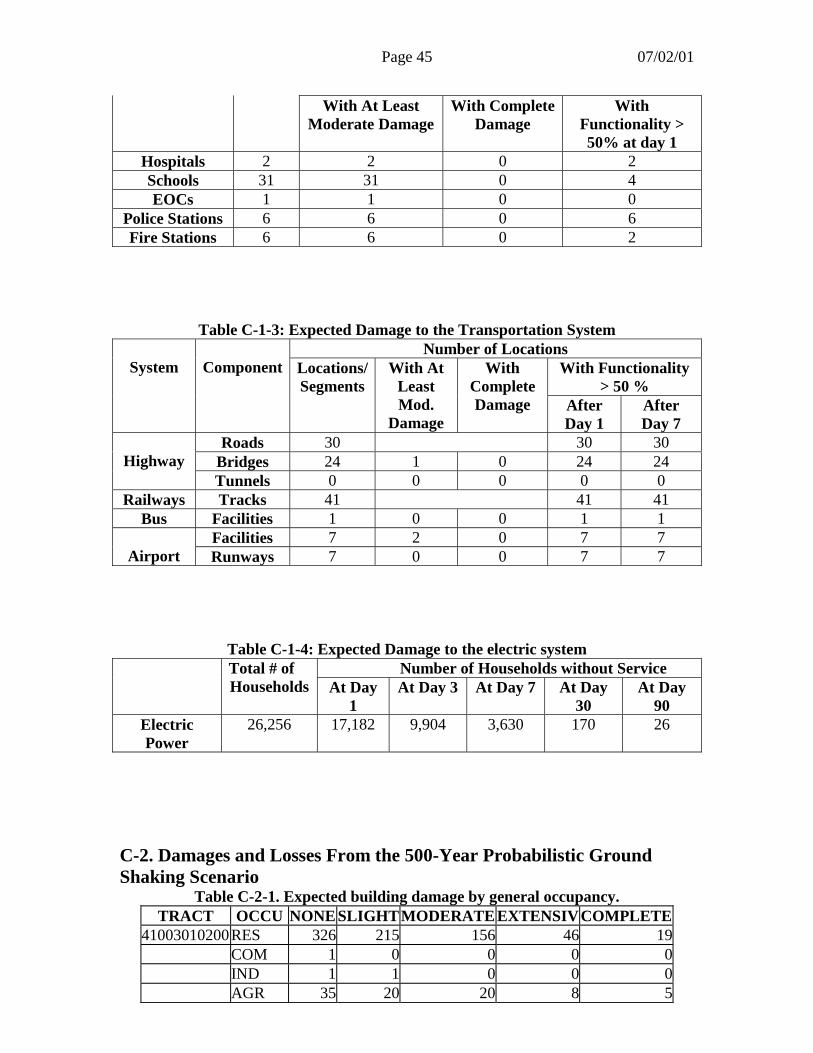
Page 45 07/02/01
With At LeastModerate Damage
With CompleteDamage
WithFunctionality >50% at day 1
Hospitals 2 2 0 2Schools 31 31 0 4EOCs 1 1 0 0
Police Stations 6 6 0 6Fire Stations 6 6 0 2
Table C-1-3: Expected Damage to the Transportation SystemNumber of Locations
With Functionality> 50 %
System Component Locations/Segments
With AtLeastMod.
Damage
WithCompleteDamage After
Day 1AfterDay 7
Roads 30 30 30Bridges 24 1 0 24 24HighwayTunnels 0 0 0 0 0
Railways Tracks 41 41 41Bus Facilities 1 0 0 1 1
Facilities 7 2 0 7 7Airport Runways 7 0 0 7 7
Table C-1-4: Expected Damage to the electric systemNumber of Households without ServiceTotal # of
Households At Day1
At Day 3 At Day 7 At Day30
At Day90
ElectricPower
26,256 17,182 9,904 3,630 170 26
C-2. Damages and Losses From the 500-Year Probabilistic GroundShaking Scenario
Table C-2-1. Expected building damage by general occupancy.TRACT OCCU NONE SLIGHTMODERATE EXTENSIVCOMPLETE
41003010200RES 326 215 156 46 19COM 1 0 0 0 0IND 1 1 0 0 0AGR 35 20 20 8 5
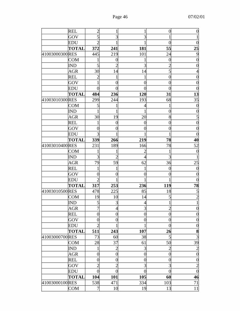
Page 46 07/02/01
REL 2 1 1 0 0GOV 5 3 3 1 1EDU 2 1 1 0 0TOTAL 372 241 181 55 25
41003000300RES 445 219 101 24 9COM 1 0 1 0 0IND 5 2 3 2 0AGR 30 14 14 5 4REL 2 1 1 0 0GOV 1 0 0 0 0EDU 0 0 0 0 0TOTAL 484 236 120 31 13
41003010300RES 299 244 193 68 35COM 5 1 4 1 0IND 1 1 1 0 0AGR 30 19 20 8 5REL 1 0 0 0 0GOV 0 0 0 0 0EDU 3 1 1 1 0TOTAL 339 266 219 78 40
41003010400RES 231 189 166 78 52COM 1 1 2 1 0IND 3 2 4 3 1AGR 79 59 62 36 25REL 1 1 1 0 0GOV 0 0 0 0 0EDU 2 1 1 1 0TOTAL 317 253 236 119 78
41003010500RES 478 225 85 18 5COM 19 10 14 5 2IND 5 3 4 1 1AGR 7 4 3 2 0REL 0 0 0 0 0GOV 0 0 0 0 0EDU 2 1 1 0 0TOTAL 511 243 107 26 8
41003000700RES 73 60 38 5 3COM 28 37 61 50 39IND 1 2 3 2 2AGR 0 0 0 0 0REL 0 0 0 0 0GOV 2 2 3 3 2EDU 0 0 0 0 0TOTAL 104 101 105 60 46
41003000100RES 538 471 334 103 71COM 7 10 19 13 11
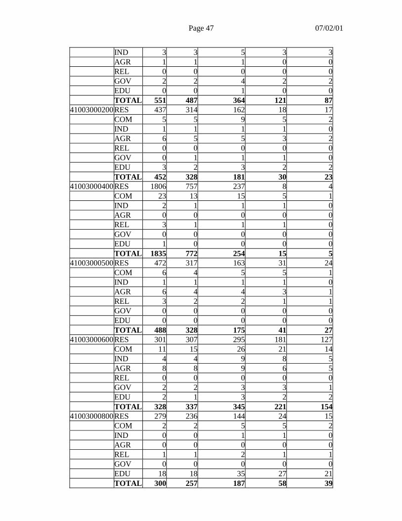
Page 47 07/02/01
IND 3 3 5 3 3AGR 1 1 1 0 0REL 0 0 0 0 0GOV 2 2 4 2 2EDU 0 0 1 0 0TOTAL 551 487 364 121 87
41003000200RES 437 314 162 18 17COM 5 5 9 5 2IND 1 1 1 1 0AGR 6 5 5 3 2REL 0 0 0 0 0GOV 0 1 1 1 0EDU 3 2 3 2 2TOTAL 452 328 181 30 23
41003000400RES 1806 757 237 8 4COM 23 13 15 5 1IND 2 1 1 1 0AGR 0 0 0 0 0REL 3 1 1 1 0GOV 0 0 0 0 0EDU 1 0 0 0 0TOTAL 1835 772 254 15 5
41003000500RES 472 317 163 31 24COM 6 4 5 5 1IND 1 1 1 1 0AGR 6 4 4 3 1REL 3 2 2 1 1GOV 0 0 0 0 0EDU 0 0 0 0 0TOTAL 488 328 175 41 27
41003000600RES 301 307 295 181 127COM 11 15 26 21 14IND 4 4 9 8 5AGR 8 8 9 6 5REL 0 0 0 0 0GOV 2 2 3 3 1EDU 2 1 3 2 2TOTAL 328 337 345 221 154
41003000800RES 279 236 144 24 15COM 2 2 5 5 2IND 0 0 1 1 0AGR 0 0 0 0 0REL 1 1 2 1 1GOV 0 0 0 0 0EDU 18 18 35 27 21TOTAL 300 257 187 58 39
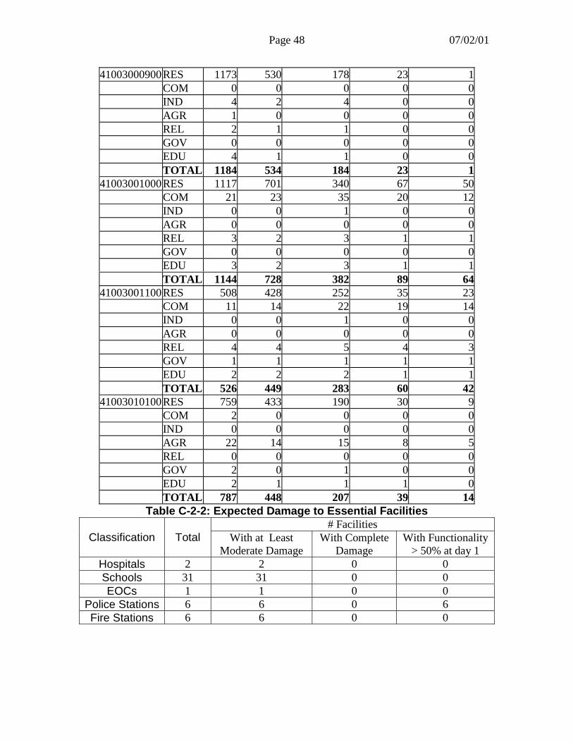
Page 48 07/02/01
41003000900RES 1173 530 178 23 1COM 0 0 0 0 0IND 4 2 4 0 0AGR 1 0 0 0 0REL 2 1 1 0 0GOV 0 0 0 0 0EDU 4 1 1 0 0TOTAL 1184 534 184 23 1
41003001000RES 1117 701 340 67 50COM 21 23 35 20 12IND 0 0 1 0 0AGR 0 0 0 0 0REL 3 2 3 1 1GOV 0 0 0 0 0EDU 3 2 3 1 1TOTAL 1144 728 382 89 64
41003001100RES 508 428 252 35 23COM 11 14 22 19 14IND 0 0 1 0 0AGR 0 0 0 0 0REL 4 4 5 4 3GOV 1 1 1 1 1EDU 2 2 2 1 1TOTAL 526 449 283 60 42
41003010100RES 759 433 190 30 9COM 2 0 0 0 0IND 0 0 0 0 0AGR 22 14 15 8 5REL 0 0 0 0 0GOV 2 0 1 0 0EDU 2 1 1 1 0TOTAL 787 448 207 39 14
Table C-2-2: Expected Damage to Essential Facilities# Facilities
Classification Total With at LeastModerate Damage
With CompleteDamage
With Functionality> 50% at day 1
Hospitals 2 2 0 0Schools 31 31 0 0EOCs 1 1 0 0
Police Stations 6 6 0 6Fire Stations 6 6 0 0
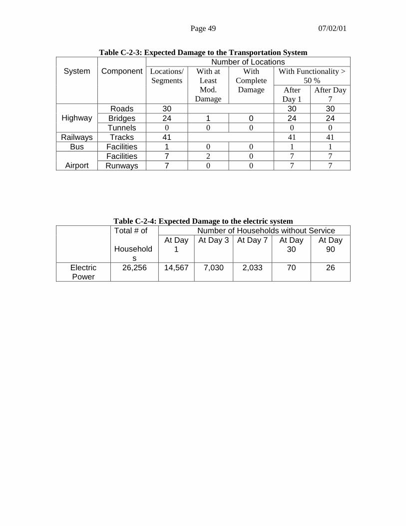
Page 49 07/02/01
Table C-2-3: Expected Damage to the Transportation SystemNumber of Locations
With Functionality >50 %
System Component Locations/Segments
With atLeastMod.
Damage
WithCompleteDamage After
Day 1After Day
7Roads 30 30 30Bridges 24 1 0 24 24HighwayTunnels 0 0 0 0 0
Railways Tracks 41 41 41Bus Facilities 1 0 0 1 1
Facilities 7 2 0 7 7Airport Runways 7 0 0 7 7
Table C-2-4: Expected Damage to the electric systemNumber of Households without ServiceTotal # of
Households
At Day1
At Day 3 At Day 7 At Day30
At Day90
ElectricPower
26,256 14,567 7,030 2,033 70 26
![IDENTIFICATION OF GEO-HAZARDS FOR THE REHABILITATION …nceg.uop.edu.pk/workshop-17to31mar-05/Slides/day17/background... · Nalbant et al [6] have postulated that movement on the](https://static.fdocuments.in/doc/165x107/5fc479ceeb89234188634b31/identification-of-geo-hazards-for-the-rehabilitation-nceguopedupkworkshop-17to31mar-05slidesday17background.jpg)