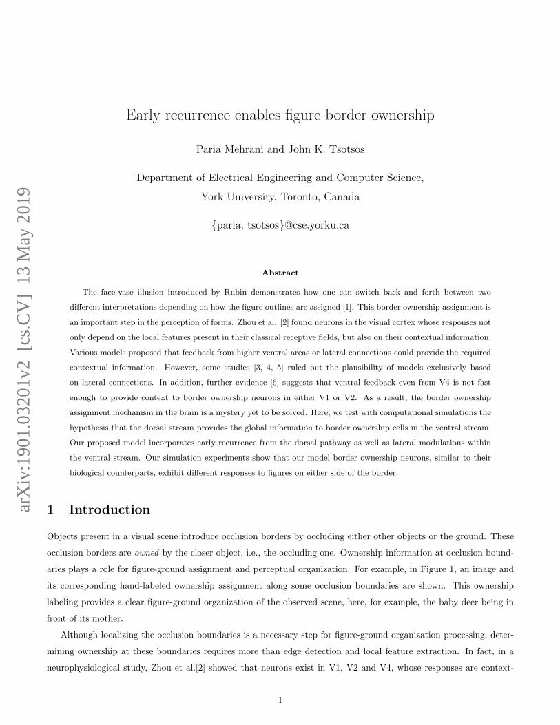
Early recurrence enables figure border ownership

Paria Mehrani and John K. Tsotsos

Department of Electrical Engineering and Computer Science,

York University, Toronto, Canada

{paria, tsotsos}@cse.yorku.ca

Abstract

The face-vase illusion introduced by Rubin demonstrates how one can switch back and forth between two

different interpretations depending on how the figure outlines are assigned [1]. This border ownership assignment is

an important step in the perception of forms. Zhou et al. [2] found neurons in the visual cortex whose responses not

only depend on the local features present in their classical receptive fields, but also on their contextual information.

Various models proposed that feedback from higher ventral areas or lateral connections could provide the required

contextual information. However, some studies [3, 4, 5] ruled out the plausibility of models exclusively based

on lateral connections. In addition, further evidence [6] suggests that ventral feedback even from V4 is not fast

enough to provide context to border ownership neurons in either V1 or V2. As a result, the border ownership

assignment mechanism in the brain is a mystery yet to be solved. Here, we test with computational simulations the

hypothesis that the dorsal stream provides the global information to border ownership cells in the ventral stream.

Our proposed model incorporates early recurrence from the dorsal pathway as well as lateral modulations within

the ventral stream. Our simulation experiments show that our model border ownership neurons, similar to their

biological counterparts, exhibit different responses to figures on either side of the border.

1 Introduction

Objects present in a visual scene introduce occlusion borders by occluding either other objects or the ground. These

occlusion borders are owned by the closer object, i.e., the occluding one. Ownership information at occlusion bound-

aries plays a role for figure-ground assignment and perceptual organization. For example, in Figure 1, an image and

its corresponding hand-labeled ownership assignment along some occlusion boundaries are shown. This ownership

labeling provides a clear figure-ground organization of the observed scene, here, for example, the baby deer being in

front of its mother.

Although localizing the occlusion boundaries is a necessary step for figure-ground organization processing, deter-

mining ownership at these boundaries requires more than edge detection and local feature extraction. In fact, in a

neurophysiological study, Zhou et al.[2] showed that neurons exist in V1, V2 and V4, whose responses are context-

1

arX

iv:1

901.

0320

1v2

[cs

.CV

] 1

3 M

ay 2

019

(a) (b)

Figure 1: (a) An example of an image from the Berkeley dataset for ownership assignment at occlusion boundariesin natural images [7, 8], (b) the corresponding human-labeled ownership assignment along some of the occlusionboundaries. In (b), white represents the side that owns the border, i.e., side of the occluding object, and black is forthe occluded region.

dependent even with identical local features in their classical receptive fields across displays. As an example, consider

the responses of a neuron from this study shown in Figure 2(a). In this figure, the little black ellipse in the middle of

each display represents the classical receptive field of the neuron, and a close look reveals the same local features in

pairs of stimuli A and B in each column. However, the context between the pairs differs in the sense that in displays of

row A, the figure is on the left side of the border, while it resides in the opposite side for all displays in row B. The bars

at the bottom of each column show the corresponding responses. For the neuron shown in this figure, the responses

are stronger to stimuli in row A with the figure on the left and weaker to stimuli in row B with the figure on the right,

for all pairs of displays presented. In other words, this neuron shows a preference to stimuli with the right side of the

figure within its receptive field and a much weaker response to those with the left side of the figure in its receptive

field. Zhou et al.[2] called this type of selectivity the side-of-figure preference and found that the context-dependent

responses of these neurons encoded ownership information at occlusion boundaries and called them border ownership

cells.

In their work, Zhou et al.[2] identified four types of border ownership neurons. Type 1 neurons showed side-of-figure

preferences, while their responses were independent of the contrast polarity on either side of the border. Responses

of one such neuron are shown in Figure 2(a). Type 2 neurons exhibited no side-of-figure preferences, but selectivity

to the local contrast polarity, while type 3 cells were selective to both side-of-figure and contrast polarity in their

receptive fields. Figure 2(b) demonstrates responses of a type 3 cell, where there are no responses to displays in

even-numbered columns with local features not matching the selectivity of this neuron. The responses to stimuli in

odd columns, however, show the preference for the figure to be on the left side of the border. Finally, neurons of type

0 demonstrated no obvious selectivity to either contrast polarity or side-of-figure features. Zhou et al.[2] also found

border ownership neurons maintain the difference of responses to figures of various sizes and changes in position of

the border within their receptive fields. When presented with solid and outlined squares, border ownership responses

were consistent across stimuli. As shown in the stimuli set for the type 3 neuron in Figure 2(b), the difference of

responses was maintained for simple as well as more complicated stimuli, such as a C-shaped figure or overlapping

2

(a) (b)

Figure 2: Responses of type 1 (a) and type 3 (b) neurons. A black ellipse shows the classical receptive field of therecorded neuron in each display. The local features within the classical receptive field of each neuron are identical ineach column of displays. The responses for both neurons, however, show a preference to stimuli with the figure on theleft, while the type 3 neuron also exhibits selectivity to contrast polarity at the border (compare responses to displaysin columns 1 and 2 of (b)). Although the large figures in (a) (columns 3-6) are not complete, according to the Gestaltprinciple of closure, these figures are to be perceived as square figures rather than holes with the rest of the image asthe figure. Plots adapted from [2].

squares. Interestingly, the average of responses to preferred and non-preferred stimuli (row A versus row B in Figure

2(a), for example) over all cells showed divergence from the beginning of stimulus onset, and the difference of responses

achieved half-peak point at about 70 ms.

Addressing the question of interactions between attentional modulation and border ownership assignment, Qiu et

al.[9] observed that attention is not required for border ownership assignment and that border ownership was assigned

for any figure in the display, both attended and ignored. However, they found that attentional enhancements were

stronger for the figure on the preferred side of the border. In an interesting work, Zhang and von der Heydt [4]

investigated the structure of the surround that provides contextual information to border ownership neurons. Their

stimuli set contained displays of fragmented Cornsweet squares1 such as those in Figure 3. While one edge was centered

on the classical receptive field, some of the rest of the fragments were occluded, and the effect of the presence or absence

of each fragment was studied. They found all fragments have a modulatory effect on the response of the neuron in

a uniform fashion, with positive and negative modulations from fragments of squares on preferred and non-preferred

sides respectively. Furthermore, they obtained weaker border ownership signals for scrambled fragmented figures such

as those presented in panel C of Figure 3.

Perhaps a prominent aspect of the study by Zhang et al.[4] is the evaluation of the plausibility of a feedforward

model with two “hot-spots”2 providing context to border ownership cells, similar to the one suggested by Sakai and

Nishimura [11]. They found that the population data does not confirm the assumption of such models. They examined

1The contours of Cornsweet figures are step edges with exponential decays on either side such that the inside of the figure has the sameintensity as the background [10]. Cornsweet stimuli allow for seamless occlusion of contour fragments.

2In their proposal, Sakai and Nishimura [11] suggested employing modulatory signals from a facilitatory region and a suppressive regionlocated asymmetrically on either side of an occlusion boundary for border ownership assignment. Zhang et al.[4] called this proposal thetwo hot-spots (facilitatory and suppressive) hypothesis.

3

Figure 3: Displays of fragmented Cornsweet figures fortesting the effect of surround providing contextual in-formation for border ownership assignments (adaptedfrom [4]). The white dashed ellipse shows the recep-tive field of the recorded neuron. Squares on eitherside of the receptive field with both contrast polaritieswere tested. Each square is divided into eight fragments,including center and corner fragments of equal length.The center fragment on one side of the figure is placed onthe receptive field. In each display, some of the remain-ing seven fragments are occluded, as some examples areshown in panel A. In a control study, the fragment cen-tered on the receptive field is occluded, with some of theother fragments present (panel B). They also recordedthe responses where the seven fragments of the squareare scrambled (panel C).

the plausibility of models with only lateral connections3, such as that of Zhaoping’s [12]. They discovered that lateral

connections could not be the only source of contextual information for border ownership assignment and a model with

both types of connections, feedback and lateral, could explain the data. Earlier, Craft et al.[3] had put forth a similar

suggestion by providing a detailed discussion on the time course of border ownership cells from the study by Zhou et

al.[2] and speed of conduction for lateral connections. This suggestion was also confirmed in a later neurophysiological

study by Sugihara et al. [5], who tested border ownership neurons with displays of small and large figures. Sugihara

et al.[5] found the latencies of border ownership cells increase for larger figures, yet are much faster to be affected by

only lateral signal propagation. They argued that the latencies of border ownership neurons in their experiments did

not rule out the possibility of a combination of feedback and lateral modulations.

Investigating the border ownership responses to occlusion boundaries in natural images, Williford and von der

Heydt [13], similar to previous studies, found that the selectivity of border ownership neurons originates from the

image context rather than the contour configuration in the classical receptive fields. Strikingly, despite the complexity

of natural images compared to the synthetic stimuli employed in previous work, the side-of-figure preference in these

neurons started to emerge at about 70 ms, a similar time course observed with synthetic displays. Following this

observation and considering the time course of IT cells reported by Brincat and Conner [14], Williford and von der

Heydt concluded that modulations from IT are not biologically plausible for border ownership assignment. In similar

research, Hesse and Tsao [15] recorded border ownership neurons in V2 and V3. Their stimuli consisted of synthetic

figures, intact natural faces as well as faces with illusory contours. In agreement with previous discoveries, these

neurons showed side-of-figure preferences at around 65 ms, with increased latencies in case of stimuli with illusory

contours.

Computational modeling of border ownership assignment was addressed in both computer vision and computational

neuroscience communities. We will review both in Section 2. We also explore two feedback possibilities for border

ownership assignment in Section 2 and argue why one is not biologically plausible by analyzing the latencies reported in

3In Zhang’s work [4], the term ”lateral connections” stands for interareal interactions between neurons with receptive fields in neighboringregions of the visual field. In computational models such as convolutional neural networks (CNNs), lateral connections are implementedusing inter- and intra-feature-map interactions of neurons within a single layer with neighboring receptive fields. A depiction of suchconnections can be found in Figure 5.

4

previous neurophysiological studies. In Section 3 our model architecture is described, as well as a detailed description of

each layer in the hierarchy. Through simulation results in Section 4, we demonstrate that our model border ownership

neurons successfully mimic the behavior of the biological ones. Then, in sections 5, we conclude the work with some

final remarks.

2 Previous work

The development of a computational model capable of determining border ownership at occlusion boundaries has been

addressed by both computer vision scientists and computational neuroscientists, but often with different objectives.

In computer vision, the goal is to have as accurate a border ownership label at occlusion boundaries as possible, by

means of computational algorithms with no constraints on biological-plausibility. The performance in such models

is usually measured against a manually-labeled dataset. In contrast, the latter approaches aim at designing models

that meet a set of known biological constraints while the simulated neurons have behavior similar to that of biological

ones, hoping to suggest a mechanism for the emergence of the observed signal in the brain. Often, the performance of

these models is judged on how well the simulated neurons replicate the behavior of their biological counterparts on a

similar set of stimuli. Sometimes, the plausibility of these models is examined with further neurophysiological studies.

In this section, we provide a review of both approaches.

2.1 Computer vision models

In computer vision, little attention has been devoted to this fundamental problem. Often, methods rely on motion and

depth information for boundary assignments [16, 17]. Inferring figure-ground organization in 2D static images was

either addressed by limiting the input to line drawings [18, 19], or by extracting local features for natural images and

applying machine learning techniques [20, 21, 22]. Usually, approaches in the latter category formulate the problem

in a conditional random field (CRF) framework to incorporate context into their model. A number of these models,

such as [20], employ shape-related features like convexity-concavity of the contour segment or local geometric class

like sky, ground, or vertical. Recently, a CNN-based model, called DOC, for figure-ground organization in a single

2D image was introduced [23]. Their network consists of two streams, one detecting edges and the other specifying

border ownership, solving a joint labeling problem. They also introduced a semi-automatic method to provide figure-

ground labeling for 20k images from the PASCAL dataset and showed superior performance over both PASCAL and

figure-ground BSD [24] dataset.

Except for methods based on low-level cues, which are not among state-of-the-art, computer vision approaches

generally attempt to solve the figure-ground organization problem by providing higher levels of features such as object

class. For example, Hoiem et al. [20] first classified each superpixel in the image as one of vertical, sky, or ground, which

provided strong priors over the object classes. In other words, these methods solve an object classification problem

prior to addressing figure-ground organization. Even in the case of the deep model dubbed as DOC, although the

network is trained on edge and occlusion boundary labels, there is no mechanism to ensure no implicit representation

of object classes is learned. Given an object class, these models mainly leverage learned statistics of how likely an

5

object is to be figure or ground. For example, the most likely event for the occlusion boundaries between any object

and sky is to be owned by the object.

To conclude, instead of solving the border ownership assignment before object recognition, these methods solve

the latter first and infer border ownership based on learned statistics. This approach is indeed a detour to addressing

the border ownership assignment problem and is in contrast to the findings about border ownership assignment. In

particular, the short latencies of border ownership cells suggest that ownership assignment happens well before any

shape processing in the ventral stream [2, 6] as we will discuss in detail in Section 2.3.

2.2 Biologically-inspired models

In the years following the border ownership study by Zhou et al.[2], there were a number of endeavors to suggest a

mechanism for border ownership assignment in the brain. For example, Zhaoping [12] proposed a model of neurons in

V1 and V2. Contextual information is provided by means of lateral connections in V2 and imposing Gestalt grouping

principles such as continuity and convexity as well as T-junction priors. Sakai and Nishimura [11] employed a vast pool

of suppression and facilitation surround neurons for this purpose. In subsequent work, Sakai et al. [25], studied the

responses of border ownership cells in this model to the complexity of shapes and found a decrease in responses with

an increase in the complexity of shapes. Later, the plausibility of these models was ruled out by the neurophysiological

findings of Zhang and von der Heydt [4]. In the same year as Zhang and von der Heydt’s work, Super et al.[26] suggest

another feedforward model based on surround suppression. An odd notion in their model is that feature maps for the

figure and background are fed as input to their two-stream network: in a sense, they provide the “answer” in advance.

The majority of computational models rely on feedback from higher layers. For example, Jehee et al.[27] introduced

a recurrent network with five areas V1, V2, V4, TEO and TE for contour extraction and border ownership computation.

Similarly, border ownership assignment in models of Layton et al.[28] and Tschechne and Neumann [29] is based on

feedback from V4 and IT. Sugihara et al.[5] as well as Williford and von der Heydt [13], however, found that the time

course of border ownership neurons does not support feedback from areas IT and beyond.

Feedback from V4 in some of the biologically-inspired models in based on responses of grouping neurons. The

earliest model, introduced by Craft et al.[3], assigns border ownership using feedback from contour grouping cells in

V4 and relies on convexity and proximity priors. Russell et al. [30] incorporated this model in a larger network and

demonstrated improvements in saliency detection. Another extension of Craft’s model [3] was introduced by Layton

and colleagues [31] with an additional layer of neurons, named R cells, with larger receptive fields than the grouping

cells in V4. Then, border ownership is a result of feedback modulations from both grouping and R neurons, as well as

imposed priors like convexity and closure. Despite the fact that no neurophysiological evidence against these models

has been found, these approaches are too dependent on shape priors such as convexity and proximity. Moreover,

they rely on feedback from grouping cells in V4 to provide the required contextual information. Nonetheless, as we

discuss in detail in the next section, the time course of V4 neuron responses does not support the suggestion of border

ownership modulations by feedback from these cells.

As a summary, the existing biologically-inspired models based on lateral connections or ventral feedback, though

replicating the behavior of biological border ownership cells, cannot provide a timely signal carrying contextual in-

6

Cell TypeTuning Component

Linear Nonlinear

Linear ∼ 65 ms ∼ 75 msMixed linear/nonlinear ∼ 63 ms ∼ 90 msAverage ∼ 65 ms ∼ 85 ms

Table 1: Time course of linear and nonlinear response components for predominantly linear and mixed linear/nonlinearcells in V4, as well as the average of all neurons (from Yau et al.[6], their Figure 5C, based on the time point of half-maximal signal strength).

formation to border ownership neurons. As a result, the border ownership encoding process in the brain remains

unclear.

2.3 Exploring feedback possibilities

Border ownership neurons reach half-peak strength for the difference of responses at about 69 ms and 68 ms in V1 and

V2 respectively, and the divergence of responses to preferred and non-preferred stimuli was observed from the beginning

of stimulus onset [2]. In this section, we examine two possibilities for providing the contextual information required

for the exhibition of this divergence: first, ventral feedback from visual area V4, and second, dorsal modulations from

MT. Neurons in both V4 and MT have receptive fields larger than those of V1 and V2 and could provide the required

contextual information to border ownership cells.

A number of studies showed that neurons in V4 exhibit selectivity to curvature [32, 33, 34]. Yau et al.[6] examined

the dynamics of curvature processing in V4 using a stimulus set of contour fragments, each with two orientation

components forming various angles of curvature. Each contour fragment was presented at 8 orientations. Their contour

tuning model consisted of linear and nonlinear terms; the linear term of the tuning accounts for the selectivity of each

neuron to its orientation components, while the nonlinear responses represent shape (convexity/concavity) selectivity.

In this study, they categorized cells as predominantly linear, predominantly nonlinear, and mixed linear/nonlinear

neurons. A summary of the time course for each of the linear/nonlinear components of the tunings are shown in Table

1. Apparent from this table is that neither linear nor mixed linear/nonlinear neurons in V4 are fast enough to provide

contextual information to border ownership cells in either V1 or V2, and this is the case for both linear and nonlinear

components of responses. In other words, a feedback signal from V4 could not be the carrier of contextual information

for the border ownership signal when it reaches its half-maximal point, let alone from the beginning of stimulus onset.

The V4 cells, however, might be part of the mechanism that enhances the difference of responses to reach its peak or

when there are ambiguities in the scene. In light of the time course of neurons in V4, models based on feedback from

V4 described above are not biologically plausible, not only because even linear responses in V4 are not fast enough,

but also due to the fact that these models rely on shape priors such as convexity, which emerge at a much later time

in V4, after 75 ms.

Another possibility for contextual modulation of border ownership neurons is MT in the dorsal pathway. A study

on V4 and MT neurons by Maunsell [35] showed much shorter latencies in MT compared to V4, reaching half-maximal

response strength at about 39 ms (their Figure 2.4, at half-maximal signal strength). MT cells not only have shorter

latencies but also have large receptive fields, comparable to those of V4, which makes them perfect candidates to

7

provide context to border ownership neurons. In fact, MT is one of the three regions that Bullier [36] called the

“fast brain” with cells that are “activated sufficiently early to influence neurons in areas V1 and V2”. It is worth

emphasizing that the early divergence in the difference of responses in border ownership neurons could be attributed to

the short latencies in MT cells. As a matter of fact, Hupe et al. [37] showed that inactivating MT would affect neurons

in areas V1, V2, and V3 to the extent that some neurons in these areas were silenced entirely in the absence of signals

from MT. This effect was pronounced in the case of figure-ground stimuli, suggesting signals from MT contribute

to figure-ground segregation. In another study, Hupe et al. [38] found that signals from MT significantly affected

responses of V1 neurons early on in the time course of responses and they concluded that these feedback connections

are employed very early for the purpose of visual processing. Inspired by these observations, in the following section,

we introduce a model of border ownership computation based on dorsal recurrent and ventral lateral modulations.

3 Our Model

In this work, we introduce a biologically plausible model for border ownership. Specifically, we introduce a model

meeting known biological properties of the relevant brain regions, while suggesting a mechanistic computation of

border ownership in the brain. Furthermore, a computer vision scientist can view our computational model as a

convolutional neural network (CNN) with certain constraints. The architecture of this network is depicted in Figure

4, while Figure 5 represents an example of lateral connections in the output layer of this architecture. In the current

work, horizontal and vertical orientations are implemented, with the goal of adding more variety of orientations to the

model in future. Each layer of neurons is modeled at four spatial scales.

The goal of our work is to model border ownership neurons of types 1 and 3, classified by Zhou et al.[2]. That is,

neurons selective to side-of-figure and not contrast polarity (type 1) and those selective to both features (type 3). To

this end, simple and complex cells in the ventral stream selective to contrast polarity and bars, from here on referred

to as border- and edge-selective neurons respectively, encode local features as well as orientation within their classical

receptive fields. These cells are responsible for signaling the existence of a border/edge to border ownership (BOS)

cells. In our model, for each complex cell, border- and edge-selective alike, two border ownership neurons with the

same orientation and local feature selectivity but opposite side-of-figure preferences are defined. For example, for a

complex cell selective to edges at orientation θ, we will have two border ownership neurons Bθ+π2

and Bθ−π2 , one

preferring the figure to reside on the right side of the edge and the other on the left side (see Figure 6). As a result,

the final number of BOS cells for each visual field location is 2×N ×S×C, where N is the number of orientations, S

is the number of local feature selectivities in the model, and C represents the number of scales. In our current model,

we have S = 4 for edge- and border-selective neurons each at two opposite contrast polarities, for example, borders

between dark-light and light-dark regions, N = 2 for horizontal and vertical orientations, and C = 4.

MT cells, carrying contextual information due to their large receptive fields, modulate border ownership neurons.

Each border ownership cell, edge- or border-selective alike, receives the dorsal modulation from the MT cells on its

preferred side. These MT cells notify the border ownership cell of the existence of prominent features on that side.

For example, consider the BOS cell in Figure 7 with figure preference on the right side, indicated by the red arrow.

8

stimulus(input)

Feedforward signalModulatory signal

VentralSimpleCells

VentralComplex

Cells

DorsalSimpleCells

MTCells

BorderOwnership

Cells

Output

Dorsal Stream

Ventral Stream

Figure 4: Border ownership network architecture. Eachscale, in both ventral and dorsal streams, defines an inde-pendent path from that of other scales. Border ownershipneurons, in the ventral stream, receive a feedforward signalfrom complex cells, and a modulatory signal, showed withblue arrows, from MT neurons. In this network, scale selec-tion is performed in the last layer, where border ownershipneurons with the same selectivity across scales are com-bined. Finally, relaxation labeling, implementing ventrallateral connections, is performed on the neurons in the out-put layer to provide local context. Ventral lateral modula-tions happen between spatially neighboring neurons withina map as well as those across maps of similar local featureselectivities. An example of such ventral lateral connectionsis depicted in Figure 5.

Figure 5: An example of the lateral connections for asingle neuron, depicted as a big red circle, in the out-put layer of our model. The connections in this exam-ple are between neurons selective to dark bars on lightregions at all orientations and ownership directions.The selectivity of each set of neurons is depicted insquares next to the set, with the red arrow indicat-ing the ownership direction selectivity. Through it-erations of relaxation labeling, these neurons interactwith the big red neuron in excitatory or inhibitorymanners and provide the local neighborhood consen-sus to this neuron. For a similar pictorial exampleof relaxation labeling for edge detection, we refer thereader to [39], their Figure 10.2.

9

Figure 6: An example of anocclusion boundary orientedat θ degrees with two direc-tions for two border owner-ship neurons each selectiveto figure on one side of theborder.

BOS cell receptive fieldSide preference

Modulating surround on the left side of a vertical border

Modulating surround on the right side of a vertical borderModulatory Connection

Figure 7: Two pools of border ownership cells for each visual field location encodethe ownership at the border. A red arrow indicates the side preference of each BOScell. Each border ownership cell receives a modulatory signal from MT cells on itspreferred side. For example, the BOS cell with side preference to the right receivesa modulatory signal from MT neurons with receptive fields in the pink surroundarea. These MT neurons notify the border ownership cell of prominent features onthat side. The dorsal modulatory signal is computed as a Gaussian weighted sumof MT responses, which is indicated using a gradient filling in each surround area.

This neuron receives signals from the on- and off-center MT cells on the right side of the border, the surround area

shown in pink. Most of the MT cells in the pink surround region are strongly activated due to the figure on that side

and send a strong modulatory signal to the border ownership cell. In contrast, the modulation signal the BOS cell

with the opposite ownership direction preference receives from the surround indicated in green is close to zero due to

absence of conspicuous features.

The size of the surround determines the number of MT cells modulating each BOS cell. Moreover, the weight of

the modulatory signal from each MT cell is computed as a Gaussian function of the distance between the receptive

field centers of the MT and BOS cells. In other words, the closer an MT cell to a border ownership neuron, the

stronger its modulatory effect on that neuron. In Figure 7, the weighting is reflected by a gradient filling in each

surround region. Finally, after dorsal modulations, in the last layer of the network, scale selection over neurons with

similar selectivities is performed.

Once an initial preference of border ownership is established, neighboring BOS neurons modulate each other by

employing relaxation labeling [39]. In particular, these lateral connections are another source for providing contextual

information, this time, in the form of local context, and enforce collinearity for border ownership. In Figure 5, the

structure of lateral connections for relaxation labeling is presented. Each BOS neuron has a network of connections to

other BOS cells at spatially neighboring visual field locations. In such a network of connections, when a BOS neuron

has a strong response in one direction while its immediate neighbors believe otherwise, the confidence of its response

is decreased and corrected over relaxation labeling iterations.

This type of computation providing local context employs lateral connections between BOS neurons, but cannot be

the only source of contextual information for border ownership assignments [4]. Nevertheless, an increase in latencies

for larger figures observed by Sugihara et al.[5] could be described by a time-limited lateral modulation. As a summary,

10

the final BOS activations are obtained from a combination of feedforward signals as well as dorsal and ventral lateral

modulations. In what follows, we describe each cell type employed in our model in detail.

Ventral simple and complex cells. Following Rodrıguez-Sanchez and Tsotsos [40], we implemented ventral

simple cells with edge selectivity using difference of Gaussians (DoG). For parameter values of DoGs, we refer the

interested readers to [40]. Border-selective simple cells in the ventral stream were implemented using Gabor filters,

g(x, y;λ, θ, ψ, σ, r) = exp

(−x′2 + r2y′2

2σ2

)cos

(2πx′

λ+ ψ

)(1)

with r = 0.5, λ = 0.2, ψ = ±π2 for two settings of contrast polarity, and σ = RF4 , where RF is short for receptive field

size. We measured 1◦ visual angle at 50 cm to be 32 pixels for stimuli size of 400 × 400 pixels, and set the ventral

simple cell receptive fields at four scales to [0.4◦, 0.6◦, 0.8◦, 1◦], following the observations of [41, 42]. Complex cells,

as in [40], were computed by a Gaussian-weighted sum of simple cells. Both types of cells are half-wave rectified. In

our implementation, all receptive fields are square-shaped, even though round shapes might be used in some of the

figures in this document in a figurative manner.

Dorsal simple cells and MT cells. The dorsal pathway is well-known to be selective to spatiotemporal features.

However, a number of neurophysiological studies [43, 44, 45, 46] provided evidence that the dorsal area MT also

responds to static stimuli. In our implementation, we skip the temporal aspect of dorsal responses as our input to the

network are static images. But such an extension is straightforward.

Angelucci et al.[41] found V1 cells receiving signal from Magnocellular (M) and Parvocellular (P) cells in the LGN

have different receptive field sizes. Neurons on the M-path have larger receptive fields and as a result, our dorsal simple

cells have receptive field sizes [0.9◦, 1.33◦, 1.76◦, 2.2◦]. In our implementation, we set the parameters of edge-selective

dorsal simple neurons as: σy = RF,WR = 2.5, AR = WR ∗ [10, 9, 8, 7], where WR is the width ratio and AR the

aspect ratio of the DoG kernel (See [40] for details). For the border-selective dorsal simple cells, the difference of two

Gaussians with σy = RF, σx =σyAR were employed. At each visual field location, the dorsal simple cell with maximum

activity feed to MT cells.

The receptive fields of MT neurons were determined based on the findings of Fiorani et al.[47], set to [2.5◦, 3.26◦,

4.02◦, 4.78◦]. Felleman and Kass [46] found that MT cells, with on and off excitatory regions, showed an increase

of responses to bars with the length up to the receptive field size. However, the effective bar width is 110 -th of the

receptive field size. In fact, for MT neurons with 4◦ receptive fields, the most effective bar width was about 0.25◦. In

other words, MT cells are selective to long narrow bars, with length matching the receptive field size. The receptive

field of an example model MT cell with such selectivities and an excitatory region in the middle is depicted in Figure

8(a). Such a receptive field profile is not unusual in the visual system as a similar one was suggested in cat simple

cells by Hubel [48] (their “SIMPLE CORTICAL CELLS” figure, subfigures a and b). We called these MT cells with

the on area in the middle as “on-center” MT neurons and implemented these cells using the Difference of Gaussians

formulation. We also implemented MT cells with an inhibitory region in the middle and two excitatory areas on the

sides, similar to Hubel’s subfigure f in his “SIMPLE CORTICAL CELLS” figure. An example of a model off-center

11

(a) on-center (b) off-center

Figure 8: Receptive fields of on-center andoff-center MT cells. The on-center MTneurons have an on area in the middle(red color) and two off regions on the sides(blue color). The kernel of off-center MTcells comprises of two excitatory (red color)Gaussians with same parameters centeredat the two sides of the kernel and one Gaus-sian with inhibitory effects (blue color) atthe center.

MT neuron receptive field is shown in Figure 8(b). Note that these neurons exhibit selectivity to long and narrow

bars on either side of the receptive field with strong activations when two bars are present on both excitatory areas.

We refer to these neurons as “off-center” MT cells, which were computed by the difference of three Gaussians, two

with same parameters centered at the two sides of the receptive field, and one centered in the middle. While the

activation of on-center MT cells signifies the existence of edges, off-center MT neurons indicate a pair of edges on

either side of their receptive fields. As a result, the sum of off-center MT neurons at all orientations will be large for

closed shapes, a key feature for border ownership assignment. For MT cells, we set σy = RF, AR = [33, 52, 80, 126.6],

and WR = [3.3, 5.2, 8, 12.6] for the four scales of receptive fields.

Various studies of the Magnocellular pathway (Shapley et al.[49], Kaplan and Shapley [50]), and MT recordings

of macaque (Sclar et al.[51]) and humans (Tootell et al. [52]), suggested that these neurons are highly sensitive to

contrast, whereas this sensitivity in V1 neurons is much lower. Tootell et al.[52] observed that reliable responses in MT

were obtained at low contrasts, and that the responses were saturated at high contrasts (higher than 1.6%). Figure

9(a), adapted from Tootell et al.[52], compares the responses of V1 and MT neurons to gratings of various contrast.

Following these observations, we employ the rectification function:

Φ =1− e−R/ρ

1 + 1/Γe−R/ρ, (2)

for dorsal neurons, where R indicates cell response. Figure 9(b) depicts this rectifier for Γ = 0.001, ρ = 0.02.

Border ownership cells. Border ownership neurons receive a feedforward signal from complex cells and a

modulatory signal from MT cells. The initial border ownership signal is determined by:

Bθ±π2 (x, y) = Cθ(x, y) · [∑d1,d2

w(d1, d2)(∑φ

MT ON(x, y, φ, d1) +∑φ

MT OFF(x, y, φ, d2))] (3)

where x, y specify the receptive field center. Complex cell responses, Cθ, are multiplicatively modulated by on-center

and off-center MT cells, represented as MT ON and MT OFF respectively, selective to orientation φ. The responses of

orientation-selective MT cells are summed to account for all the possible orientations, φ, of the figure contour segment

12

(a) (b)

Figure 9: MT cells show high sensitivity to contrast. (a) Comparison of MT and V1 contrast sensitivity in humans.Figure adapted from Tootell et al.[52]. (b) The rectification function Φ as a function of contrast, for parameter valuesΓ = 0.001, ρ = 0.02. This rectifier ensures high contrast sensitivity in the dorsal stream.

opposite to the occlusion boundary. In addition, d1, d2 parameters determine the center of receptive fields for the MT

cells with respect to that of the border ownership neuron, and w(·, ·) is a linear weighting function with a negative

slope, assigning larger weights for MT cells with receptive fields closer to the occlusion boundary. Note that each

modulation term obtained by expanding the outer summation in Equation 3 (∑d1,d2

) is indeed a manifestation of the

isotropic inhibition proposed by Shi et al.[53] since each term is a weighted multiplicative process with weights set to 1

for all orientations. The outer sum, here, integrates isotropic modulatory responses at multiple visual field locations.

Now the question is how large is the surround for BOS cells? In other words, what should be the extent of region

from which MT neurons provide context to the BOS cells (i.e., parameters d1 and d2 in Equation 3)? Studying the

extent of surround for V1 and V2 neurons, Shushruth et al. [54] discovered that the far surround could exceed 12.5

degrees, on average about 5.5 degrees for V1 and 9.2 degrees for V2. In a similar study, Angelucci and Bullier [55]

observed a similar extent of surround for neurons in V1. They tested the effect of feedback from both V2 and MT

and observed that surround size could get as big as 13 times the size of V1 receptive fields, and concluded that

MT neurons could provide these long-distance interactions. Accordingly, we set the extent of surround for border

ownership neurons provided by MT cells to a maximum of 9◦, 13 times the average model V1 receptive field size.

Relaxation Labeling

After computing the initial border ownership responses, a few iterations of relaxation labeling can provide local

context and ensure smoothness in responses [39]. In this step, the set of border ownership neurons with receptive fields

corresponding to a single visual field location comprise the set of labels associated with that location. The neighboring

relationship defined over the visual field locations determines the local region that provides context to border ownership

cells. Figure 5 illustrates the neighboring relationship in our implementation. An important component of relaxation

labeling is the compatibility function between the set of labels, which determines the influence of context on a label

at a visual field location and also affects the strength of this influence. In our implementation, a Gaussian function

13

has been employed for compatible labels to highly reward matching labels, with a sharp fall as the labels become

less similar. The penalty for incompatible labels, such as those with the same local feature selectivities but opposite

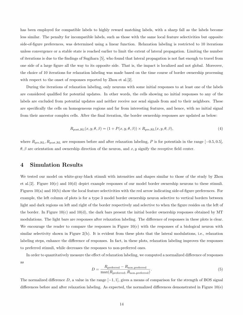
side-of-figure preferences, was determined using a linear function. Relaxation labeling is restricted to 10 iterations

unless convergence or a stable state is reached earlier to limit the extent of lateral propagation. Limiting the number

of iterations is due to the findings of Sugihara [5], who found that lateral propagation is not fast enough to travel from

one side of a large figure all the way to its opposite side. That is, the impact is localized and not global. Moreover,

the choice of 10 iterations for relaxation labeling was made based on the time course of border ownership processing

with respect to the onset of responses reported by Zhou et al.[2].

During the iterations of relaxation labeling, only neurons with some initial responses to at least one of the labels

are considered qualified for potential updates. In other words, the cells showing no initial responses to any of the

labels are excluded from potential updates and neither receive nor send signals from and to their neighbors. These

are specifically the cells on homogeneous regions and far from interesting features, and hence, with no initial signal

from their ancestor complex cells. After the final iteration, the border ownership responses are updated as below:

Rpost RL(x, y, θ, β) = (1 + P (x, y, θ, β))×Rpre RL(x, y, θ, β), (4)

where Rpre RL, Rpost RL are responses before and after relaxation labeling, P is for potentials in the range [−0.5, 0.5],

θ, β are orientation and ownership direction of the neuron, and x, y signify the receptive field center.

4 Simulation Results

We tested our model on white-gray-black stimuli with intensities and shapes similar to those of the study by Zhou

et al.[2]. Figure 10(c) and 10(d) depict example responses of our model border ownership neurons to these stimuli.

Figures 10(a) and 10(b) show the local feature selectivities with the red arrow indicating side-of-figure preferences. For

example, the left column of plots is for a type 3 model border ownership neuron selective to vertical borders between

light and dark regions on left and right of the border respectively and selective to when the figure resides on the left of

the border. In Figure 10(c) and 10(d), the dark bars present the initial border ownership responses obtained by MT

modulations. The light bars are responses after relaxation labeling. The difference of responses in these plots is clear.

We encourage the reader to compare the responses in Figure 10(c) with the responses of a biological neuron with

similar selectivity shown in Figure 2(b). It is evident from these plots that the lateral modulations, i.e., relaxation

labeling steps, enhance the difference of responses. In fact, in these plots, relaxation labeling improves the responses

to preferred stimuli, while decreases the responses to non-preferred ones.

In order to quantitatively measure the effect of relaxation labeling, we computed a normalized difference of responses

as

D =Rpreferred −Rnon preferred

max(Rpreferred, Rnon preferred). (5)

The normalized difference D, a value in the range [−1, 1], gives a means of comparison for the strength of BOS signal

differences before and after relaxation labeling. As expected, the normalized differences demonstrated in Figure 10(e)

14

(a) (b)

(c) (d)

(e) (f)

(g) (h)

Figure 10: Example of model border ownership responses to stimuli used in the neurophysiological experiments byZhou et al.[2]. (a) and (b) represent the selectivity of neurons for which responses are shown in columns of this figure.The red arrows show the border ownership direction selectivity. In (c) and (d), dark bars indicate the initial borderownership responses obtained by MT modulations, and the light bars show the responses after relaxation labeling.Compare the responses in (c) with the responses of a biological neurons shown in Figure 2(b). In (e) and (f), thenormalized differences, i.e., the relative amount of difference in responses to preferred and non-preferred stimuli aredepicted. In (g) and (h), the percentage of improvement after relaxation labeling is shown.

and 10(f), are larger after relaxation labeling compared to MT-modulated responses. To measure the amount of

enhancement by lateral modulations, improvement percentage for before vs. after relaxation labeling was computed.

As can be seen in Figure 10(g) and 10(h), more than 100% improvement over the initial difference of responses is

observed. This pattern of improvement was also seen in our other model border ownership neurons, which are not

included here for brevity. The interested reader can find those responses in Appendix A.

15

(a)

(b) (c)

Figure 11: Position invariance in border ownership responses. (a) Selectivity of a model border ownership cell whichposition invariance in its responses are shown in (b). (c) Position invariance in biological border ownership neuronresponses (adapted from [2]). In (b) and (c), the side of figure is aligned to the orientation selectivity of the neuron.

Zhou et al.[2] found position invariance in responses when they moved the figure perpendicular to the border.

Similarly, we tested the position invariance property in our model neurons. Figure 11 depicts the responses of a model

neuron to changes in position. One example from the neurophysiological experiment [2] is included in this figure for

comparison. The responses of our model border ownership cells to changes in position are comparable to those of

the biological neurons, with a peak of responses when the border is located at the center of the receptive field, and

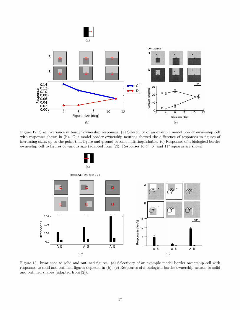
a decrease in responses when it moves away from the center. In terms of sensitivity to figure size, the difference of

responses was observed in the neurophysiological experiments up to a figure size that the figure and ground were

indistinguishable. Our model neurons exhibited a similar behavior to square figures of various sizes, as shown in

Figure 12. Likewise, our model neurons demonstrated the difference of responses to both solid and outlined figures,

as depicted in Figure 13.

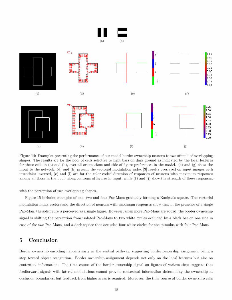
The length and direction of the vector obtained from the vectorial modulation index (VMI) introduced by Craft et

al.[3] describes the strength and side-of-figure direction of the border ownership signal utilizing a vector. For a couple

of examples of overlapping shapes, the performance of our model border ownership cells is demonstrated in Figure

14. These examples include the responses of the pool of border ownership neurons, selective to all the implemented

orientations and side-of-figure preferences with local feature selectivities shown in 14(a) and 14(b). The first column

in each row shows the input to the network, and the second column is VMI vectors overlayed on the input with

inverted intensities. The third and fourth columns in this figure are for the direction and signal strength of the border

ownership cell with maximum response among the neurons in the pool. These examples show that even though we

imposed no priors over shape or T-junctions and no feedback from V4, the border ownership signals are in agreement

16

(a)

(b) (c)

Figure 12: Size invariance in border ownership responses. (a) Selectivity of an example model border ownership cellwith responses shown in (b). Our model border ownership neurons showed the difference of responses to figures ofincreasing sizes, up to the point that figure and ground become indistinguishable. (c) Responses of a biological borderownership cell to figures of various size (adapted from [2]). Responses to 4◦, 6◦ and 11◦ squares are shown.

(a)

(b) (c)

Figure 13: Invariance to solid and outlined figures. (a) Selectivity of an example model border ownership cell withresponses to solid and outlined figures depicted in (b). (c) Responses of a biological border ownership neuron to solidand outlined shapes (adapted from [2]).

17

(a) (b)

(c) (d) (e) (f)

(g) (h) (i) (j)

Figure 14: Examples presenting the performance of our model border ownership neurons to two stimuli of overlappingshapes. The results are for the pool of cells selective to light bars on dark ground as indicated by the local featuresfor these cells in (a) and (b), over all orientations and side-of-figure preferences in the model. (c) and (g) show theinput to the network, (d) and (h) present the vectorial modulation index [3] results overlayed on input images withintensities inverted, (e) and (i) are for the color-coded direction of responses of neurons with maximum responsesamong all those in the pool, along contours of figures in input, while (f) and (j) show the strength of these responses.

with the perception of two overlapping shapes.

Figure 15 includes examples of one, two and four Pac-Mans gradually forming a Kanizsa’s square. The vectorial

modulation index vectors and the direction of neurons with maximum responses show that in the presence of a single

Pac-Man, the sole figure is perceived as a single figure. However, when more Pac-Mans are added, the border ownership

signal is shifting the perception from isolated Pac-Mans to two white circles occluded by a black bar on one side in

case of the two Pac-Mans, and a dark square that occluded four white circles for the stimulus with four Pac-Mans.

5 Conclusion

Border ownership encoding happens early in the ventral pathway, suggesting border ownership assignment being a

step toward object recognition. Border ownership assignment depends not only on the local features but also on

contextual information. The time course of the border ownership signal on figures of various sizes suggests that

feedforward signals with lateral modulations cannot provide contextual information determining the ownership at

occlusion boundaries, but feedback from higher areas is required. Moreover, the time course of border ownership cells

18

(a) (b) (c) (d)

(e) (f) (g) (h)

(i) (j) (k) (l)

(m) (n) (o) (p)

Figure 15: Examples presenting the performance of our model border ownership neurons to one, two and four Pac-Mans present in the stimuli. The results are for the pool of cells selective to borders between light and dark regionsat horizontal and vertical orientations and all BOS direction selectivities shown in (a), (b), (c), and (d). Figures (e),(i), and (m) show the input to the network. The vectorial modulation index results overlayed on input images withintensities inverted are presented in (f), (j), and (n). In (g), (k), and (o), the direction of responses of neurons withmaximum responses among all those in the pool, along contours of figures in input, are depicted. The directions inthese figures are color-coded. Finally, (h), (l), and (p) present the strength of these responses. In the example of asingle Pac-Man, the direction of BOS responses with maximum response shown in (g) clearly shows that the borderownership direction for the the two edge components of the concavity are correctly assigned except for the very cornerof the concavity. In other words, the border ownership cells see an isolated figure in stimuli. However, the directionof this assignment gradually changes when two and later four Pac-Mans are present in the display, as depicted in (k)and (o).

and those of IT neurons indicate that feedback from IT is not fast enough to provide context for BOS cells. Likewise,

here, we described neurophysiological evidence suggesting that V4 is not fast enough in terms of both linear and

19

nonlinear processing components to send a timely feedback signal to border ownership cells.

Inspired by these observations, we introduced a hierarchical model that not only replicates the behavior of biological

BOS cells but, in contrast to previous models, is also biologically plausible and could describe the mechanism the brain

employs for border ownership assignment. This was achieved through early recurrence from the dorsal stream, which

could very well describe the observed difference of responses in biological border ownership cells from the beginning

of stimulus onset. Aside from fast latencies in the dorsal stream, neurons in this pathway are highly sensitive to

spatiotemporal variations at coarser scales compared to those of the ventral stream and are less sensitive to contrast.

As a result, the signal from the dorsal stream becomes more robust to noise and low contrasts at occlusion boundaries.

These two characteristics of MT cells and their short latencies make them perfect candidates for providing contextual

information to border ownership cells. Previously, early recurrence from the dorsal stream showed improvements in

low-level feature representations [56] and edge detection [53]. In a similar attempt, we demonstrated the role of early

recurrence from the dorsal stream in providing global information essential for even higher levels of abstraction, i.e.,

border ownership assignment.

Another novel aspect of our model is combining global and local context. Although the global information provided

by MT cells results in a border ownership assignment, it does not warrant that the border ownership directions are

consistent among neighboring visual field locations. The relaxation labeling step in our algorithm implementing lateral

connections among border ownership cells ensures consistent labeling in local regions. Our results clearly demonstrate

an enhancement in the border ownership signal after a few iterations of relaxation labeling. The improvement in

response differences to preferred and non-preferred stimuli was more than 100% after relaxation labeling. Additionally,

this step could describe the gradual increase in the difference of responses as the iterations of relaxation labeling

provide local support with a lag to border ownership neurons, due to the time required for the signal to travel in a

local neighborhood.

In our simulation results, we demonstrated that our model neurons of types 1 and 3 show side-of-figure preferences

similar to those of biological cells, and are invariant to position, size and solid/outlined figures. Furthermore, when

presented with overlapping shapes, our model BOS cells assign borders to the occluding figure along the occlusion

boundaries. Interestingly, in the experiment with Pac-Mann figures, the borders are assigned to the Pac-Man in case

of a single figure, and then to an illusory occluding shape with the gradual addition of more Pac-Mans to form the

Kanizsa’s square.

The current model is limited to horizontal and vertical orientations and one step to further improve this model is

to implement a variety of orientations. Zhou et al.[2] reported border ownership cells selective to color borders and

designed their stimuli to match the selectivity of those neurons. Another future attempt is to add color borders to

our model. Moreover, we would like to test the performance of our model to more complex stimuli such as randomly

generated overlapping polygonal scenes and real images. A natural extension to our model would be learning the

set of free parameters in our network, such as kernel parameters in each layer and the extent of surround for border

ownership neurons.

As a final remark, although neurophysiological evidence regarding latencies as well as our experimental results

support the hypothesis of dorsal and lateral modulations for border ownership assignment, it will be insightful to

20

examine this hypothesis on biological cells. One possible experiment is to remove any feedback from the dorsal

stream to these neurons. By removing the dorsal effect, the border ownership assignment would have to be based on

feedforward and lateral connections, a hypothesis that has already been ruled out [4, 5]. As a result, we expect the

border ownership neurons to have no explicit representation of the ownership assignment at occlusion boundaries.

6 Acknowledgments

This research was supported by several sources for which the authors are grateful: Air Force Office of Scientific Re-

search (FA9550-14-1-0393), the Canada Research Chairs Program, and the Natural Sciences and Engineering Research

Council of Canada.

References

[1] E. Rubin, Synsoplevede figurer: studier i psykologisk analyse. Første del.-1915.-xii, 228 pp., ill., tabl. Gyldendal,

1915.

[2] H. Zhou, H. S. Friedman, and R. von der Heydt, “Coding of border ownership in monkey visual cortex,” Journal

of Neuroscience, vol. 20, no. 17, pp. 6594–6611, 2000.

[3] E. Craft, H. Schutze, E. Niebur, and R. von der Heydt, “A neural model of figure–ground organization,” Journal

of Neurophysiology, vol. 97, no. 6, pp. 4310–4326, 2007.

[4] N. R. Zhang and R. von der Heydt, “Analysis of the context integration mechanisms underlying figure–ground

organization in the visual cortex,” Journal of Neuroscience, vol. 30, no. 19, pp. 6482–6496, 2010.

[5] T. Sugihara, F. T. Qiu, and R. von der Heydt, “The speed of context integration in the visual cortex,” Journal

of Neurophysiology, vol. 106, no. 1, pp. 374–385, 2011.

[6] J. M. Yau, A. Pasupathy, S. L. Brincat, and C. E. Connor, “Curvature processing dynamics in macaque area v4,”

Cerebral Cortex, 2012.

[7] C. C. Fowlkes, D. R. Martin, and J. Malik, “Local figure–ground cues are valid for natural images,” Journal of

Vision, vol. 7, no. 8, pp. 2–2, 2007.

[8] X. Ren, C. C. Fowlkes, and J. Malik, “Figure/ground assignment in natural images,” in European Conference on

Computer Vision, pp. 614–627, Springer, 2006.

[9] F. T. Qiu, T. Sugihara, and R. Von Der Heydt, “Figure-ground mechanisms provide structure for selective

attention,” Nature neuroscience, vol. 10, no. 11, p. 1492, 2007.

[10] T. N. Cornsweet, Visual perception. Academic Press, 1970.

[11] K. Sakai and H. Nishimura, “Surrounding suppression and facilitation in the determination of border ownership,”

Journal of Cognitive Neuroscience, vol. 18, no. 4, pp. 562–579, 2006.

21

[12] L. Zhaoping, “Border ownership from intracortical interactions in visual area {V2},” Neuron, vol. 47, no. 1,

pp. 143 – 153, 2005.

[13] J. R. Williford and R. von der Heydt, “Figure-ground organization in visual cortex for natural scenes,” eneuro,

vol. 3, no. 6, pp. ENEURO–0127, 2016.

[14] S. L. Brincat and C. E. Connor, “Dynamic shape synthesis in posterior inferotemporal cortex,” Neuron, vol. 49,

no. 1, pp. 17 – 24, 2006.

[15] J. K. Hesse and D. Y. Tsao, “Consistency of border-ownership cells across artificial stimuli, natural stimuli, and

stimuli with ambiguous contours,” Journal of Neuroscience, vol. 36, no. 44, pp. 11338–11349, 2016.

[16] H. Fu, C. Wang, D. Tao, and M. J. Black, “Occlusion boundary detection via deep exploration of context,” in

Proceedings of the IEEE Conference on Computer Vision and Pattern Recognition, pp. 241–250, 2016.

[17] P. Sundberg, T. Brox, M. Maire, P. Arbelaez, and J. Malik, “Occlusion boundary detection and figure/ground

assignment from optical flow,” in Computer Vision and Pattern Recognition (CVPR), 2011 IEEE Conference on,

pp. 2233–2240, IEEE, 2011.

[18] M. Nitzberg and D. Mumford, “The 2.1-d sketch,” in [1990] Proceedings Third International Conference on

Computer Vision, pp. 138–144, Dec 1990.

[19] L. G. Roberts, Machine perception of three-dimensional solids. PhD thesis, Massachusetts Institute of Technology,

1963.

[20] D. Hoiem, A. A. Efros, and M. Hebert, “Recovering occlusion boundaries from an image,” International Journal

of Computer Vision, vol. 91, no. 3, pp. 328–346, 2011.

[21] X. Ren, C. C. Fowlkes, and J. Malik, “Figure/ground assignment in natural images,” in Proceedings of the 9th

European conference on Computer Vision-Volume Part II, pp. 614–627, Springer-Verlag, 2006.

[22] C. C. Fowlkes, D. R. Martin, and J. Malik, “Local figure–ground cues are valid for natural images,” Journal of

Vision, vol. 7, no. 8, pp. 2–2, 2007.

[23] P. Wang and A. Yuille, DOC: Deep OCclusion Estimation from a Single Image, pp. 545–561. Cham: Springer

International Publishing, 2016.

[24] D. Martin, C. Fowlkes, D. Tal, and J. Malik, “A database of human segmented natural images and its application

to evaluating segmentation algorithms and measuring ecological statistics,” in Proc. 8th Int’l Conf. Computer

Vision, vol. 2, pp. 416–423, July 2001.

[25] K. Sakai, H. Nishimura, R. Shimizu, and K. Kondo, “Consistent and robust determination of border ownership

based on asymmetric surrounding contrast,” Neural Networks, vol. 33, pp. 257–274, 2012.

[26] H. Super, A. Romeo, and M. Keil, “Feed-forward segmentation of figure-ground and assignment of border-

ownership,” PLOS ONE, vol. 5, pp. 1–14, 05 2010.

22

[27] J. F. Jehee, V. A. Lamme, and P. R. Roelfsema, “Boundary assignment in a recurrent network architecture,”

Vision Research, vol. 47, no. 9, pp. 1153 – 1165, 2007.

[28] O. W. Layton, E. Mingolla, and A. Yazdanbakhsh, “Neural dynamics of feedforward and feedback processing in

figure-ground segregation,” Frontiers in Psychology, vol. 5, p. 972, 2014.

[29] S. Tschechne and H. Neumann, “Hierarchical representation of shapes in visual cortex—from localized features

to figural shape segregation,” Frontiers in Computational Neuroscience, vol. 8, p. 93, 2014.

[30] A. F. Russell, S. Mihalas, R. von der Heydt, E. Niebur, and R. Etienne-Cummings, “A model of proto-object

based saliency,” Vision Research, vol. 94, pp. 1 – 15, 2014.

[31] O. W. Layton, E. Mingolla, and A. Yazdanbakhsh, “Dynamic coding of border-ownership in visual cortex,”

Journal of Vision, vol. 12, no. 13, p. 8, 2012.

[32] A. Pasupathy and C. E. Connor, “Responses to contour features in macaque area v4,” J. Neurophysiol, pp. 2490–

2502, 1999.

[33] A. Pasupathy and C. E. Connor, “Population coding of shape in area v4,” Nature neuroscience, vol. 5, no. 12,

pp. 1332–1338, 2002.

[34] A. Pasupathy and C. E. Connor, “Shape representation in area v4: position-specific tuning for boundary confor-

mation,” Journal of neurophysiology, vol. 86, no. 5, pp. 2505–2519, 2001.

[35] J. H. Maunsell, “Physiological evidence for two visual subsystems,” in Matters of intelligence, pp. 59–87, Springer,

1987.

[36] J. Bullier, “Integrated model of visual processing,” Brain Research Reviews, vol. 36, no. 2, pp. 96–107, 2001.

[37] J. Hupe, A. James, B. Payne, S. Lomber, P. Girard, and J. Bullier, “Cortical feedback improves discrimination

between figure and background by v1, v2 and v3 neurons,” Nature, vol. 394, no. 6695, pp. 784–787, 1998.

[38] J.-M. Hupe, A. C. James, P. Girard, S. G. Lomber, B. R. Payne, and J. Bullier, “Feedback connections act on

the early part of the responses in monkey visual cortex,” Journal of neurophysiology, vol. 85, no. 1, pp. 134–145,

2001.

[39] S. W. Zucker, “Relaxation labeling: 25 years and still iterating,” in Foundations of Image Understanding, pp. 289–

321, Springer, 2001.

[40] A. J. Rodrıguez-Sanchez and J. K. Tsotsos, “The roles of endstopped and curvature tuned computations in a

hierarchical representation of 2d shape,” PLoS ONE, vol. 7, pp. 1–13, 08 2012.

[41] A. Angelucci, J. B. Levitt, and J. S. Lund, “Anatomical origins of the classical receptive field and modulatory

surround field of single neurons in macaque visual cortical area v1,” in Progress in brain research, vol. 136,

pp. 373–388, Elsevier, 2002.

23

[42] R. Gattass, A. P. Sousa, and M. G. Rosa, “Visual topography of v1 in the cebus monkey,” Journal of Comparative

Neurology, vol. 259, no. 4, pp. 529–548, 1987.

[43] T. D. Albright, “Direction and orientation selectivity of neurons in visual area mt of the macaque,” Journal of

neurophysiology, vol. 52, no. 6, pp. 1106–1130, 1984.

[44] S. Raiguel, D.-K. Xiao, V. Marcar, and G. Orban, “Response latency of macaque area mt/v5 neurons and its

relationship to stimulus parameters,” Journal of Neurophysiology, vol. 82, no. 4, pp. 1944–1956, 1999.

[45] H. Kolster, R. Peeters, and G. A. Orban, “The retinotopic organization of the human middle temporal area mt/v5

and its cortical neighbors,” Journal of Neuroscience, vol. 30, no. 29, pp. 9801–9820, 2010.

[46] D. J. Felleman and J. H. Kaas, “Receptive-field properties of neurons in middle temporal visual area (mt) of owl

monkeys,” Journal of Neurophysiology, vol. 52, no. 3, pp. 488–513, 1984.

[47] M. Fiorani Jr, R. Gattass, M. G. Rosa, and A. P. Sousa, “Visual area mt in the cebus monkey: location, visuotopic

organization, and variability,” Journal of Comparative Neurology, vol. 287, no. 1, pp. 98–118, 1989.

[48] D. H. Hubel, “The visual cortex of the brain,” Scientific American, vol. 209, no. 5, pp. 54–63, 1963.

[49] R. Shapley, E. Kaplan, and R. Soodak, “Spatial summation and contrast sensitivity of x and y cells in the lateral

geniculate nucleus of the macaque,” Nature, vol. 292, no. 5823, p. 543, 1981.

[50] E. Kaplan and R. M. Shapley, “The primate retina contains two types of ganglion cells, with high and low contrast

sensitivity,” Proceedings of the National Academy of Sciences, vol. 83, no. 8, pp. 2755–2757, 1986.

[51] G. Sclar, J. H. Maunsell, and P. Lennie, “Coding of image contrast in central visual pathways of the macaque

monkey,” Vision research, vol. 30, no. 1, pp. 1–10, 1990.

[52] R. B. Tootell, J. B. Reppas, K. K. Kwong, R. Malach, R. T. Born, T. J. Brady, B. R. Rosen, and J. W. Belliveau,

“Functional analysis of human mt and related visual cortical areas using magnetic resonance imaging,” Journal

of Neuroscience, vol. 15, no. 4, pp. 3215–3230, 1995.

[53] X. Shi, B. Wang, and J. K. Tsotsos, “Early recurrence improves edge detection.,” in BMVC, 2013.

[54] S. Shushruth, J. M. Ichida, J. B. Levitt, and A. Angelucci, “Comparison of spatial summation properties of

neurons in macaque v1 and v2,” Journal of neurophysiology, vol. 102, no. 4, pp. 2069–2083, 2009.

[55] A. Angelucci and J. Bullier, “Reaching beyond the classical receptive field of v1 neurons: horizontal or feedback

axons?,” Journal of Physiology-Paris, vol. 97, no. 2, pp. 141–154, 2003.

[56] X. Shi, N. D. Bruce, and J. K. Tsotsos, “Biologically motivated local contextual modulation improves low-level

visual feature representations,” in International Conference Image Analysis and Recognition, pp. 79–88, Springer,

2012.

24

Appendix A

Here, we provide the responses of our model neurons to stimuli employed in the neurophysiological study by Zhou et

al.[2], similar to those shown in Figure 10.

(a) (b)

(c) (d)

(e) (f)

(g) (h)

Figure 16: Example of model border ownership responses to stimuli used in the neurophysiological experiments byZhou et al.[2]. (a) and (b) represent the selectivity of neurons for which responses are shown in columns of this figure.The red arrows show the border ownership direction selectivity. In (c) and (d), dark bars indicate the initial borderownership responses obtained by MT modulations, and the light bars show the responses after relaxation labeling. In(e) and (f), the normalized differences, i.e., the relative amount of difference in responses to preferred and non-preferredstimuli are depicted. In (g) and (h), the percentage of improvement after relaxation labeling is shown.

25

(a) (b)

(c) (d)

(e) (f)

(g) (h)

Figure 17: Example of model border ownership responses to stimuli used in the neurophysiological experiments byZhou et al.[2]. (a) and (b) represent the selectivity of neurons for which responses are shown in columns of this figure.The red arrows show the border ownership direction selectivity. In (c) and (d), dark bars indicate the initial borderownership responses obtained by MT modulations, and the light bars show the responses after relaxation labeling. In(e) and (f), the normalized differences, i.e., the relative amount of difference in responses to preferred and non-preferredstimuli are depicted. In (g) and (h), the percentage of improvement after relaxation labeling is shown.

26

(a) (b)

(c) (d)

(e) (f)

(g) (h)

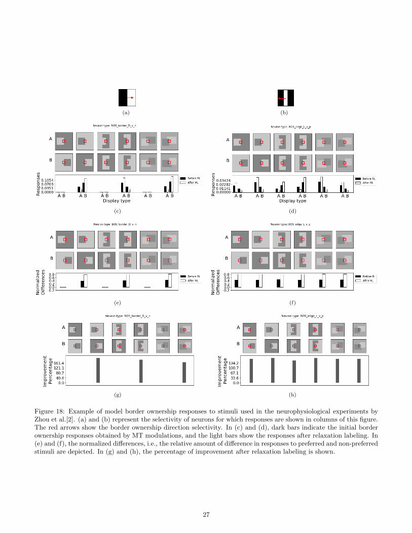
Figure 18: Example of model border ownership responses to stimuli used in the neurophysiological experiments byZhou et al.[2]. (a) and (b) represent the selectivity of neurons for which responses are shown in columns of this figure.The red arrows show the border ownership direction selectivity. In (c) and (d), dark bars indicate the initial borderownership responses obtained by MT modulations, and the light bars show the responses after relaxation labeling. In(e) and (f), the normalized differences, i.e., the relative amount of difference in responses to preferred and non-preferredstimuli are depicted. In (g) and (h), the percentage of improvement after relaxation labeling is shown.

27

(a) (b)

(c) (d)

(e) (f)

(g) (h)

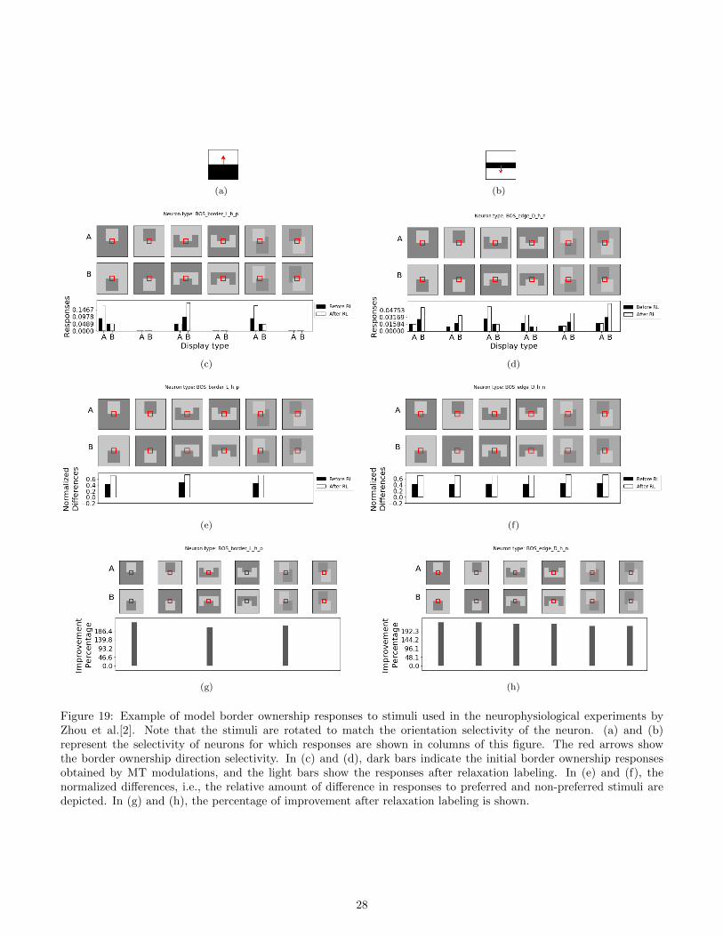
Figure 19: Example of model border ownership responses to stimuli used in the neurophysiological experiments byZhou et al.[2]. Note that the stimuli are rotated to match the orientation selectivity of the neuron. (a) and (b)represent the selectivity of neurons for which responses are shown in columns of this figure. The red arrows showthe border ownership direction selectivity. In (c) and (d), dark bars indicate the initial border ownership responsesobtained by MT modulations, and the light bars show the responses after relaxation labeling. In (e) and (f), thenormalized differences, i.e., the relative amount of difference in responses to preferred and non-preferred stimuli aredepicted. In (g) and (h), the percentage of improvement after relaxation labeling is shown.

28

(a) (b)

(c) (d)

(e) (f)

(g) (h)

Figure 20: Example of model border ownership responses to stimuli used in the neurophysiological experiments byZhou et al.[2]. Note that the stimuli are rotated to match the orientation selectivity of the neuron. (a) and (b)represent the selectivity of neurons for which responses are shown in columns of this figure. The red arrows showthe border ownership direction selectivity. In (c) and (d), dark bars indicate the initial border ownership responsesobtained by MT modulations, and the light bars show the responses after relaxation labeling. In (e) and (f), thenormalized differences, i.e., the relative amount of difference in responses to preferred and non-preferred stimuli aredepicted. In (g) and (h), the percentage of improvement after relaxation labeling is shown.

29

(a) (b)

(c) (d)

(e) (f)

(g) (h)

Figure 21: Example of model border ownership responses to stimuli used in the neurophysiological experiments byZhou et al.[2]. Note that the stimuli are rotated to match the orientation selectivity of the neuron. (a) and (b)represent the selectivity of neurons for which responses are shown in columns of this figure. The red arrows showthe border ownership direction selectivity. In (c) and (d), dark bars indicate the initial border ownership responsesobtained by MT modulations, and the light bars show the responses after relaxation labeling. In (e) and (f), thenormalized differences, i.e., the relative amount of difference in responses to preferred and non-preferred stimuli aredepicted. In (g) and (h), the percentage of improvement after relaxation labeling is shown.

30

(a) (b)

(c) (d)

(e) (f)

(g) (h)

Figure 22: Example of model border ownership responses to stimuli used in the neurophysiological experiments byZhou et al.[2]. Note that the stimuli are rotated to match the orientation selectivity of the neuron. (a) and (b)represent the selectivity of neurons for which responses are shown in columns of this figure. The red arrows showthe border ownership direction selectivity. In (c) and (d), dark bars indicate the initial border ownership responsesobtained by MT modulations, and the light bars show the responses after relaxation labeling. In (e) and (f), thenormalized differences, i.e., the relative amount of difference in responses to preferred and non-preferred stimuli aredepicted. In (g) and (h), the percentage of improvement after relaxation labeling is shown.

31