Early estimations of dimensions for prestressed concrete ...
91
Early estimations of dimensions for prestressed concrete bridges Optimization by Set-based Parametric Design of Cross-Section and Prestressing Force in a Preliminary Stage Master’s thesis in Master Programme Structural Engineering & Building technology DANIEL ASPEGREN ERIK MÖÖRK Department of Architecture and Civil Engineering Division of Structural Engineering Concrete Structures CHALMERS UNIVERSITY OF TECHNOLOGY Gothenburg, Sweden 2021 www.chalmers.se
Transcript of Early estimations of dimensions for prestressed concrete ...

Early estimations of dimensions for prestressed concrete bridges Optimization by Set-based Parametric Design of Cross-Section and Prestressing Force in a Preliminary Stage
Master’s thesis in Master Programme Structural Engineering & Building technology
DANIEL ASPEGREN ERIK MÖÖRK
Department of Architecture and Civil Engineering Division of Structural Engineering Concrete Structures
CHALMERS UNIVERSITY OF TECHNOLOGY Gothenburg, Sweden 2021
www.chalmers.se

MASTER’S THESIS ACEX30
Early Estimations of Dimensions for Prestressed Concrete
Bridges
Optimization by Set-Based Parametric Design of Cross-Section and Prestressing Force
in a Preliminary Stage
Master’s Thesis in the Master’s Programme Structural Engineering and Building
Technology
DANIEL ASPEGREN
ERIK MÖÖRK
Department of Architecture and Civil Engineering
Division of Structural Engineering
Concrete structures
CHALMERS UNIVERSITY OF TECHNOLOGY
Gothenburg, Sweden 2021

Early Estimations of Dimensions for Prestressed Concrete Bridges
Optimization by Set-Based Parametric Design of Cross-Section and Prestressing Force in
a Preliminary Stage
Master’s Thesis in the Master’s Programme Structural Engineering and Building
Technology
DANIEL ASPEGREN
ERIK MÖÖRK
© DANIEL ASPEGREN, ERIK MÖÖRK 2021
Examensarbete ACEX30
Institutionen för Arkitektur och Samhällsbyggnadsteknik
Chalmers tekniska högskola, 2021
Department of Architecture and Civil Engineering
Division of Structural Engineering
Concrete Structures
Chalmers University of Technology
SE-412 96 Göteborg
Sweden
Telephone: + 46 (0)31-772 1000
Cover: Picture of FE model in BRIGADE/Plus of studied two-span continuous
prestressed concrete bridge, showing the sectional moment distribution.
Department of Architecture and Civil Engineering
Gothenburg, Sweden, 2021

I
Early Estimations of Dimensions for Prestressed Concrete Bridges
Optimization by Set-Based Parametric Design of Cross-Section and Prestressing Force
in a Preliminary Stage
Master’s Thesis in the Master’s Programme Structural Engineering and Building
Technology
DANIEL ASPEGREN
ERIK MÖÖRK
Department of Architecture and Civil Engineering
Division of Structural Engineering
Concrete Structures
Chalmers University of Technology
ABSTRACT
When designing concrete bridges, estimations of the dimensions and reinforcement
content are made to estimate the cost of the bridge in an early phase. When the final
bridge is designed, the estimated dimensions based on experience and simplification is
often used and checked against the national regulations. If the dimensions comply with
the regulations, the estimated design is used as the final design and there is not often
time to reduce and optimize the dimensions to make the bridge more material efficient.
This master thesis presents an optimization method for the early estimations of the
design for continuous prestressed concrete bridges. This method is based on set-based
parametric design and the optimization is performed with a python script where this
method is implemented. The optimization is focusing on the relationship between beam
height, number of prestressed tendons and the parabolic tendon layout with the aim to
minimize the global warming potential (GWP) and cost for the superstructure. The
script with the optimization method has been created to enable an effective approach to
reach an optimized solution in the preliminary design phase, which will result in a more
material efficient final bridge design.
To reach the lowest GWP and cost, a slender cross-section with a large number of
prestressed tendons is desirable. Depending on the case-specific conditions, the tendon
layout is preferable designed in different ways. For shorter bridges, a tendon layout that
is minimizing the secondary moment is preferable to obtain a slender cross-section,
while for longer bridges the self-weight is increased and therefore a tendon layout that
results in a larger secondary moment is the most favourable.
The method was used to create designs which was compared with two existing bridges
designed by Inhouse Tech Göteborg AB. The designs showed an improvement, for both
cost and GWP compared to the existing bridges. Above all, there are opportunities for
a more optimized and material-efficient design if the tendon layout is adapted to the
case specific conditions.
Key words: Prestressed concrete bridge, Preliminary design, Set-based parametric
design, BRIGADE/Plus, Tendon layout, Optimization

II
Uppskattning av dimensioner för förspända broar i tidiga skeden
Optimering av tvärsnitt och förspänningskraft genom Set-Based Parametric Design i
preliminärdimensioneringsfasen
Examensarbete inom masterprogrammet Structural Engineering and Building
Technology
DANIEL ASPEGREN
ERIK MÖÖRK
Institutionen för arkitektur och samhällsbyggnadsteknik
Avdelningen för konstruktionsteknik
Betongbyggnad
Chalmers tekniska högskola
SAMMANFATTNING
Vid utformning av förspända betongbroar görs en tidig uppskattning av dimensionerna
och armeringsinnehållet för att uppskatta kostnaden för bron. Vid utformningen av den
slutliga bron används ofta de dimensioner som uppskattats i tidigt skede, baserat på
erfarenhet och antaganden mot de nationella bestämmelserna. Om brodesignen
uppfyller reglerna används denna utformning för den slutgiltiga bron och det finns ofta
inte tid att minska och optimera materialanvändningen i bron.
Detta examensarbete presenterar en optimeringsmetod för de tidiga uppskattningarna
av utformningen hos kontinuerliga förspända betongbroar. Denna metod baseras på set-
based parametric design och optimeringen utförs med hjälp av en python-kod där denna
optimeringsmetod är implementerad. Optimeringen fokuserar på förhållandet mellan
balkhöjd, antal förspända kablar samt den paraboliska kabelföringen i syfte att
minimera den globala uppvärmningspotentialen (GWP) och kostnad för
överbyggnaden. Python-koden har skapats för att möjliggöra ett effektivt och
användarvänligt tillvägagångssätt för att nå en optimerad lösning i
preliminärdimensioneringen och resulterar därför i en mer materialeffektiv slutlig
brodesign.
För lägsta miljöpåverkan och kostnad, är ett lågt tvärsnitt med ett stort antal förspända
kablar önskvärt. Beroende på de specifika förhållandena för varje bro är det fördelaktigt
att utforma kabelföringen på olika sätt. För kortare broar är en kabelföring som
minimerar tvångsmomentet mest optimalt för att få ett minimerat tvärsnitt, men för
längre broar ökar egenvikten och därför är en kabelföring som resulterar i ett större
tvångsmoment det mest gynnsamma.
Metoden användes för att ta fram utformningar som jämfördes med två befintliga broar
konstruerade av Inhouse Tech Göteborg AB. Utformningarna visar en förbättring
avseende både kostnad och GWP jämfört med de befintliga broarna. Framför allt finns
det möjligheter till en mer optimerad och materialeffektiv lösning om kabelföringen
anpassas till de projektspecifika förutsättningarna.
Nyckelord: Förspända betongbro, Preliminärdimensionering, Kabelföring, Optimering

CHALMERS Architecture and Civil Engineering, Master’s Thesis ACEX30 III
Contents
ABSTRACT I
SAMMANFATTNING II
CONTENTS III
PREFACE V
LIST OF FIGURES VI
LIST OF TABLES VIII
NOTATIONS IX
1 INTRODUCTION 1
1.1 Background 1
1.2 Aim and Objectives 1
1.3 Limitations 2
1.4 Methodology 2
2 DESIGN OF PRESTRESSED CONCRETE BRIDGES 3
2.1 Continuous post-tensioned bridge 3 2.1.1 The aim of prestressing 3
2.1.2 Post-tensioning 3 2.1.3 Tendon layout 4
2.1.4 Long term effects 6
2.2 Loads 7
2.2.1 Traffic loads 7 2.2.2 Load combinations 9
2.3 Preliminary design 11
2.3.1 Prestressing and reinforcement steel 11 2.3.2 Ultimate limit state 12
2.3.3 Service limit state 13 2.3.4 Accidental limit state – Rupture of prestressing steel 14
2.4 FE modelling of concrete structures 14
2.5 Cost and global warming potential for the materials 15
3 PARAMETRIC DESIGN 17
3.1 Parametric modelling 17
3.2 Parametric optimization 17
4 PARAMETRIC MODELLING FOR PRESTRESSED BRIDGE 20
4.1 Tendon Layout 20

CHALMERS Architecture and Civil Engineering, Master’s Thesis ACEX30 IV
4.2 FINITE ELEMENT MODEL 22
4.2.1 Geometry and element types 23 4.2.2 Tie connections 26
4.2.3 Boundary conditions 27 4.2.4 Mesh size – Convergence study 28 4.2.5 FE-model verification 30
4.3 FINITE ELEMENT MODEL LOADS 31 4.3.1 Permanent loads 31
4.3.2 Variable loads 32 4.3.3 Load groups and combinations 35
5 OPTIMIZATION WITH SET-BASED PARAMETRIC DESIGN 36
5.1 Optimization of beam height 36
5.2 Optimization of the tendon layout 36
5.3 Optimization for number of tendons 36
5.4 Evaluation method and design checks 38
5.5 Entire optimization 40
6 RESULTS 41
6.1 Relation between beam height and number of tendons 43
6.2 Minimum beam height for different span lengths 45
6.3 Effect of chosen beam width and maximum number of tendons 46
6.4 Comparison to existing bridges 49
6.4.1 Bridge 100-411-1 49 6.4.2 Bridge 100-412-1 52
7 DISCUSSION 55
7.1 General Results 55
7.2 Comparison to two existing bridges 56
7.3 Simplifications 58
8 CONCLUSION 59
8.1 Further investigations 60
9 REFERENCES 61
APPENDICES 63

CHALMERS Architecture and Civil Engineering, Master’s Thesis ACEX30 V
Preface
This Master’s Thesis has been carried out at the division of Structural Engineering at
Chalmers University of Technology as the final work in the master’s program Structural
Engineering and Building Technology. The thesis has been performed in collaboration
with Inhouse Tech Göteborg AB.
We would like to thank our supervisors Oscar Yman and Max Fredriksson from Inhouse
Tech Göteborg AB for their support and input during the work of this thesis, and for
their enthusiasm and quick response despite the special conditions of the covid
pandemic. Thanks also to Isak Svensson at Inhouse Tech Göteborg AB for your python
guidance and to Göran Hannrup at PEAB for your quick and effective expertise in
labour and material cost of concrete bridges.
We would also like to thank our examinator and supervisor, Mario Plos at Chalmers
University of Technology for his input on FE modelling and feedback on the project.
Göteborg, June 2021
Daniel Aspegren
Erik Möörk

CHALMERS Architecture and Civil Engineering, Master’s Thesis ACEX30 VI
List of Figures
Figure 2.1 - Principal design of the studied bridge. ....................................................... 3
Figure 2.2 - Effect of anchorage slip on the prestressing force. Based on Engström
(2011b). .......................................................................................................................... 4
Figure 2.3 - Common tendon profile with eccentricity e(x). ......................................... 5
Figure 2.4 - Principle for how the secondary moment's Ms is generated. Based on Dolan
and Hamilton (2019) ...................................................................................................... 5
Figure 2.5 - Placement of load fields. Based on SIS, 2003a. ......................................... 8
Figure 2.6 - Load placement in LM1 according to Eurocode 1. Based on SIS, 2003a. 9
Figure 2.7 - Stress-strain diagrams for ULS design adapted from Eurocode 2 (SIS,
2005a). ......................................................................................................................... 12
Figure 2.8 – Strain relationship for prestressed concrete section. ............................... 13
Figure 3.1 - Simplified flow chart of the design process for a normal reinforced concrete
bridge and a prestressed concrete bridge. .................................................................... 18
Figure 4.1 - Coordinates for input to generate tendon layout in the FE model. .......... 20
Figure 4.2 - Secondary moment for an 8m wide bridge with 36m spans with different
eccentricities in the span. Distance presented for the different eccentricities is the
distance from the bottom of the beam to the centre of the tendon. .............................. 21
Figure 4.3 - Case study of how the moment capacity follows the sectional moment for
different values of L0. .................................................................................................. 22
Figure 4.4 - Shape of the bridge from the FE model, including the bridge deck. ....... 23
Figure 4.5 - Shape of the bridge from the FE model, excluding the bridge deck to show
the different beams and the tendon. ............................................................................. 24
Figure 4.6 - Illustration of the wingwall design ........................................................... 26
Figure 4.7 - Tie connection between bridge deck and beam. Picture from
BRIGADE/Plus. ........................................................................................................... 26
Figure 4.8 - Tie connection between edge beam and bridge deck. Picture from
BRIGADE/Plus. ........................................................................................................... 27
Figure 4.9 - Placement of boundary conditions. Image from BRIGADE/Plus. .......... 27
Figure 4.10 - Illustration of the support behaviours. Translational degrees of freedom.
Bridge seen from above ............................................................................................... 28
Figure 4.11 - Moment diagram for different element sizes. ........................................ 29
Figure 4.12 - Support moment error for a different number of elements in the main
beam ............................................................................................................................. 29
Figure 4.13 - Model used in hand calculations. ........................................................... 30
Figure 4.14 - Bending moment in the main beam for different load models, including
LM1 (SIS, 2003a) and national vehicle models (Trafikverket, 2019a). Due to symmetry
only half of the bridge is displayed. ............................................................................. 33

CHALMERS Architecture and Civil Engineering, Master’s Thesis ACEX30 VII
Figure 4.15 - Maximum and minimum moment for different settings on the increment.
...................................................................................................................................... 35
Figure 5.1 – Illustration of the optimization approach to obtain a minimum number of
tendons ......................................................................................................................... 38
Figure 5.2 – Flow chart of the SBPD-method design for the optimization process. ... 40
Figure 6.1 - Approved combinations of beam height and number of tendons for the two
bridges .......................................................................................................................... 44
Figure 6.2 - Cost for different beam heights with the corresponding number of tendons.
...................................................................................................................................... 44
Figure 6.3 - GWP for different beam heights with the corresponding number of tendons.
...................................................................................................................................... 45
Figure 6.4 - Minimum beam height for different span lengths for the two bridges. ... 45
Figure 6.5 - Minimum beam height for different span lengths for the different input data
for the bridge design. ................................................................................................... 47
Figure 6.6 - Cost comparison of different input data for the bridge design. ................ 48
Figure 6.7 - Comparison of GWP for different input data for the bridge design. ....... 48
Figure 6.8 - Number of tendons needed for different beam heights compared with
existing bridge. ............................................................................................................. 50
Figure 6.9 - Cost for different beam heights with the corresponding number of tendons
compared with the existing bridge. .............................................................................. 50
Figure 6.10 - GWP for different beam heights with the corresponding number of
tendons compared with the existing bridge. ................................................................ 51
Figure 6.11 - Number of tendons needed for different beam heights compared with
existing bridge. ............................................................................................................. 53
Figure 6.12 - Cost for different beam heights with the corresponding number of tendons
compared with the existing bridge. .............................................................................. 53
Figure 6.13 - GWP for different beam heights with the corresponding number of
tendons compared with the existing bridge. ................................................................ 54

CHALMERS Architecture and Civil Engineering, Master’s Thesis ACEX30 VIII
List of Tables
Table 2.1 - Number of load fields and their widths depending on total width w (SIS,
2003a). ........................................................................................................................... 8
Table 2.2 - Cost of material and work for prestressing steel ....................................... 16
Table 2.3 - Cost and C02 - equivalents for the optimized materials. ........................... 16
Table 4.1 – Verification results of FE-Model. ............................................................. 30
Table 6.1 - Fixed input in entire Chapter 6. ................................................................. 42
Table 6.2 – Bridge used for relation between beam height and the number of tendons.
...................................................................................................................................... 43
Table 6.3 - Minimum beam height for different span lengths with the corresponding
number of tendons, L0 and espan parameters. ................................................................ 46
Table 6.4 – Differences of the input for the bridges compared in Section 6.3. ........... 46
Table 6.5 – Information about the two compared bridges. .......................................... 49
Table 6.6 - Result comparison of ULS and SLS checks between the optimized and the
existing bridge. ............................................................................................................. 51
Table 6.7 – Information about the two compared bridges. .......................................... 52
Table 6.8 - Result comparison of ULS and SLS checks between the optimized and the
existing bridge. ............................................................................................................. 54
Table 6.9 – Summarization of the reduction for the cost and GWP compared to the
existing bridge designs. ................................................................................................ 54
CHALMERS Architecture and Civil Engineering, Master’s Thesis ACEX30 IX
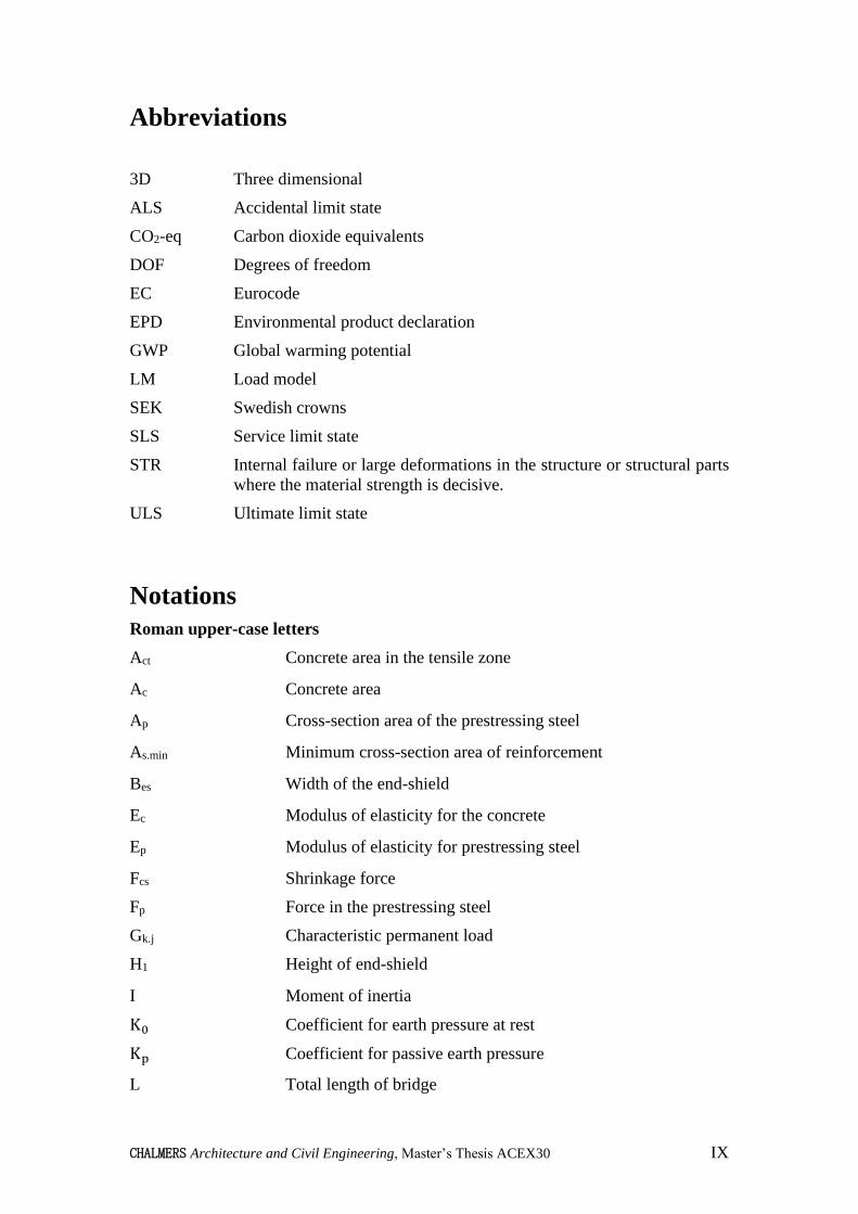
Abbreviations
3D Three dimensional
ALS Accidental limit state
CO2-eq Carbon dioxide equivalents
DOF Degrees of freedom
EC Eurocode
EPD Environmental product declaration
GWP Global warming potential
LM Load model
SEK Swedish crowns
SLS Service limit state
STR Internal failure or large deformations in the structure or structural parts
where the material strength is decisive.
ULS Ultimate limit state
Notations
Roman upper-case letters
Act Concrete area in the tensile zone
Ac Concrete area
Ap Cross-section area of the prestressing steel
As.min Minimum cross-section area of reinforcement
Bes Width of the end-shield
Ec Modulus of elasticity for the concrete
Ep Modulus of elasticity for prestressing steel
Fcs Shrinkage force
Fp Force in the prestressing steel
Gk.j Characteristic permanent load
H1 Height of end-shield
I Moment of inertia
K0 Coefficient for earth pressure at rest
Kp Coefficient for passive earth pressure
L Total length of bridge

CHALMERS Architecture and Civil Engineering, Master’s Thesis ACEX30 X
L0 Distance from the support to where the tendon is at the same
level as the centre of gravity of the cross-section
LCG Distance from the bottom of the beam to the centre of gravity
Lww Length of wingwalls
MEd Design moment
Mp Primary moment
MRd Moment capacity
Ms Secondary moment
P Prestressing force
Tshrinkage Temperature change to represent the shrinkage
Qk Characteristic point load
Qk.1 Main characteristic variable load
Qk.i Characteristic variable load
R Reaction force
Roman lower-case letters
bw Width of beam web
ccduct Centre to centre distance between tendon ducts
dp Distance from top of the beam to the centre of the prestressing
steel
e Eccentricity of the tendon from the centre of gravity
espan Maximum eccentricity of the tendon in the span
fcd Design compressive strength of concrete
fck Characteristic compressive strength of concrete
fctm Mean tensile strength of concrete
fct.eff Tensile strength of concrete when cracking occurs. Set to fctm or
lower (fctm(t)) if cracking occurs before 28 days after cast.
fp.0,1k Characteristic 0,1% strain limit for prestressing steel
fpd Design tensile capacity of prestressing steel
fpk Characteristic tensile capacity of prestressing steel
k Coefficient that compensates the impact of uneven residual
stresses in the cross-section before cracking and change of
internal level arm
kc Coefficient that considers stress distribution in the cross-section
before cracking
l Theoretical span length

CHALMERS Architecture and Civil Engineering, Master’s Thesis ACEX30 XI
n1 Number of load fields
ntendon Number of tendons
ntendon.max Maximum number of tendons
qearth.increased Increased earth pressure due to movement against earth
qearth.rest Earth pressure at rest depending on depth (z)
qk Characteristic distributed load
qself-weight Distributed load only including the self-weight
qsurcharge Surcharge load
tf Thickness of flange
w Total carriageway width
x Coordinate along the bridge
z Depth from zero-pressure level
Greek letters
αQi Adaption factor for concentrated loads
αqi Adaption factor for distributed loads
αspan Factor to decrease the eccentricity of the tendon in the span (espan)
αc Thermal expansion coefficient for concrete
γs Safety partial factor for steel
γG.j Safety partial factor for permanent loads
γQ Safety partial factor for variable loads
γp Safety partial factor for prestressing force
γ Density of the earth
δ Horizontal movement of the bridge
δmax Maximum horizontal movement
∆εp Strain in the tendons due to load effect
εcs Shrinkage strain of concrete
εp0i Initial strain of the prestressing steel
εp Total strain in tendon
εp0 Strain in the tendons due to prestressing
εcu Strain in concrete
𝜉j Reduction factor
ρmin Factor to decide minimum normal reinforcement
φ(∞, t0) Final creep coefficient [-]

CHALMERS Architecture and Civil Engineering, Master’s Thesis ACEX30 XII
σs Absolut value of the stress in the reinforcement after cracking.
Not larger than the yield stress, fyk
σp.max Maximum stress in the prestressing steel
σp.m0 Stress directly after the release of the tensioning the maximum
σcc Concrete compressive stress
σcp Concrete stress at the level of prestressing steel
σct Concrete tensile stress
χ∞ Relaxation factor after long time
Ψ0 Load combination factor
Ψ1 Load combination factor
Ψ2 Load combination factor

CHALMERS Architecture and Civil Engineering, Master’s Thesis ACEX30 1
1 Introduction
1.1 Background
In bridge design, early estimations of the dimensions and reinforcement amount are
made to estimate the cost of the bridge. The estimation is generally based upon
experience and simplified calculations. While most of the specific design regarding the
bridge is made during the detailed design phase, the dimensions are usually not
changed. Instead, the detailed design is using the dimensions from the early estimations.
This means that the amount of material for the bridge is largely decided based upon
estimations and experience instead of calculations. It is therefore a risk that a lot of
unnecessary material is used.
From a sustainable as well as an economic perspective, it is important to optimize the
structures to maximize material efficiency. In 2017, the construction industry accounted
for 19% of the Swedish greenhouse gas emissions (Boverket, 2021). Global warming
is a major concern around the world, and the Swedish construction industry has
developed a joint goal to achieve net-zero emissions in 2045 (Naturvårdsverket, 2020).
To contribute to this goal, structures should be designed with a method based on
optimization rather than experience and estimations.
1.2 Aim and Objectives
This master’s thesis aims to make the early estimations of the dimensions more accurate
than if they are based on experience and estimations only. This will result in a reduced
amount of material needed for the bridge, which is desirable from both an
environmental and an economical perspective.
The goal is to create a tool in the shape of a python script that can be used together with
the design software BRIGADE/Plus version 6.2-20 (Scanscot Technology, 2021) to
make early estimations that are more accurate for two-span prestressed concrete
bridges. The tool will be able to handle different input data, such as bridge width and
span lengths, and present a design solution that will be optimized from an economical
or environmental point of view. This will make the design more effective without being
more time-consuming than the design based on experience.
The main objectives for this thesis are:
• Identify parameters in the design with a large influence on the result.
• Develop an optimization method for the studied bridge type using set-based
parametric design.
• Design the cross-section and prestressing steel of the bridge with respect to
bending in the longitudinal direction.
• Create an optimized combination between beam height and amount of
prestressing steel concerning cost and global warming potential (GWP).
• Perform comparisons with existing bridges to evaluate the potential of the
optimization method.

CHALMERS Architecture and Civil Engineering, Master’s Thesis ACEX30 2
1.3 Limitations
• The normal reinforcement steel is not optimized or designed.
• Optimization of material will not be included; standard concrete and
prestressing steel are used.
• The design will be based on the European Standard, Eurocode (EC), and the
Swedish regulations.
1.4 Methodology
The first phase of the project was a literature study regarding both parametric design
and the theory of prestressed bridges. From this, the most important parameters for the
design were identified and the standardized method when designing this type of bridge
was studied. To get a better understanding of python scripting, an introductory course
was studied.
The next step was to create a Python script that builds a finite element (FE) model.
Python is a programming language that is used in this thesis to control the design
software BRIGADE/Plus, to do post-processing of the results from the FE analysis and
to summarize the results. BRIGADE/Plus is an FE program developed by Scanscot
(2021) for bridge design that uses ABAQUS as FE-solver. The script builds the FE
model in the design software based on parametric design to enable optimization of the
bridge and to enable the possibility to change span length, width, and other dimensions
of the bridge. The entire geometry of the bridge including wingwalls, end-shields, and
the prestressing steel is included in the model.
To verify that the model works as intended and that the assumptions and simplifications
are accurate, a comparison has been made with simplified hand calculations of a
specific load case. A convergence study of the mesh size has also been performed.
The tendon layout was designed based on the results from the literature study and an
investigation of how different parameters for the layout are affecting the structural
behaviour. The layout of the tendons is determined by a few parameters and the
combination of these parameters gives different layouts for the tendon.
The parametric optimization is focusing on finding the most efficient combination
between beam height and number of prestressing cables. Different tendon layouts are
used for each height to find an optimized solution. The method implemented in the
optimization to find this solution is based on set-based parametric design. The script
does an FE analysis and performs the required design checks according to EC for all
load combinations. The approved solutions have been evaluated and compared with
respect to their cost and GWP to achieve the most optimal solution.
The method was used to create designs for different bridges which were evaluated
through a comparison to existing bridges. This is to analyse the potential of this
optimization method and to study if the current design method can be improved such
that more material efficient bridge designs can be found.

CHALMERS Architecture and Civil Engineering, Master’s Thesis ACEX30 3
2 Design of prestressed concrete bridges
In the following chapter, the theory and design process for continuous prestressed beam
bridges is described. The behaviour, which loads that are acting on the bridge, and the
preliminary design process in current engineering practice are the focus.
2.1 Continuous post-tensioned bridge
The bridge studied in this thesis is a prestressed continuous bridge with two spans. This
is also the type of bridge that is treated in this chapter. Figure 2.1 illustrates the principal
bridge, with connected structural parts. A detailed explanation of the modelled bridge
is given in Chapter 4.
2.1.1 The aim of prestressing
When a concrete beam is subjected to bending, cracks appear at the tension side when
the stress exceeds the tension capacity of the concrete. By applying the prestressing,
the structure is exposed to a compressive normal force which leads to a delay of the
cracking in the concrete. As long as the cross-section remains uncracked, the flexural
rigidity is larger than for a cracked section, and the deflection is therefore decreased
compared to a normal reinforced concrete structure.
When estimating the size of the beam for a certain span length, l, recommendations on
the span to beam depth, h, ratios are often used. This ratio can be almost twice as large
when using prestressed concrete beams compared to normally reinforced beams
according to (Engström, 2011b). The span to depth ratio for simply supported beams
are about (𝑙/ℎ)𝑚𝑎𝑥 ≈ 20 for normal reinforced concrete beams and almost (𝑙/ℎ)𝑚𝑎𝑥 ≈ 40 for prestressed concrete beams.
2.1.2 Post-tensioning
There are two different methods for prestressing of concrete, pre-tensioning, and post-
tensioning where the prestressing steel is tensioned before and after casting of the
concrete, respectively. In this thesis, cast in-situ concrete bridges are studied. For such
bridges, post-tensioning systems are used and therefore only this method is treated here.
Figure 2.1 - Principal design of the studied bridge.

CHALMERS Architecture and Civil Engineering, Master’s Thesis ACEX30 4
When using post-tensioning in bridge constructions, ducts for the prestressing steel are
placed in the formwork. When the concrete has been cast and reached an adequate
strength, the steel is tensioned to achieve the prestressing effect (Engström, 2011b). In
practice, the tensioning is done by attaching an anchorage of the prestressing steel on
one end and a hydraulic jack on the opposite end of the concrete beam. The hydraulic
jack then tensions the steel to the desired tendon force.
When the steel at the hydraulic jack is released and anchored a phenomenon called
anchorage slip often occurs. The anchorage slip results in a drop in the tendon force,
but due to frictional forces along the tendon in the opposite direction of the tendon
force, the decrease in tendon force only occurs over a length xas closest to the edge
(Engström, 2011b). This action is illustrated in Figure 2.2.
2.1.3 Tendon layout
The most used tendon profile for continuous beams has a parabolic shape and is placed
to counteract the bending moment due to vertical loads. The profile of the prestressing
tendon is described with its eccentricity e(x) to the centreline of the beam, where x is
the coordinate along the beam. The common tendon profile for the type of continuous
beam investigated in this thesis together with its eccentricity e(x) is illustrated in Figure
2.3. The shape of the tendon profile is designed so that it follows the moment diagram
along the beam (Engström, 2011a). The resulting moment from the prestressing force,
𝑃(𝑥), multiplied with 𝑒(𝑥) is called the primary moment, Mp.
Figure 2.2 - Effect of anchorage slip on the prestressing force. Based on Engström (2011b).

CHALMERS Architecture and Civil Engineering, Master’s Thesis ACEX30 5
If the response of the tendon force with the corresponding profile in Figure 2.3 is
studied, the prestressing force wants to bend the beam upwards, giving it a negative
curvature. To prevent the beam from lifting at the mid support, a downward reaction
force, R, is generated here. Consequently, to obtain vertical equilibrium in this stage,
upward forces have to act on the two end supports (Dolan & Hamilton, 2019). These
three reaction forces will create a linear moment distribution, and this moment is called
secondary moments, Ms, illustrated in Figure 2.4.
Figure 2.3 - Common tendon profile with eccentricity e(x).
Figure 2.4 - Principle for how the secondary moment's Ms is generated. Based on
Dolan and Hamilton (2019)

CHALMERS Architecture and Civil Engineering, Master’s Thesis ACEX30 6
The effect of the secondary moment creates a complex design situation, since 𝑃(𝑥) ∗𝑒(𝑥) often is designed to counteract the sectional moment from the external load effect,
𝑀𝐸𝑑.𝑞(𝑥). The complexity comes from that the final sectional moment, 𝑀𝐸𝑑(𝑥), is
including 𝑀𝐸𝑑.𝑞(𝑥) but also an addition from the secondary moment Ms which is
unknown until both the tendon force P and the eccentricity e is decided.
2.1.4 Long term effects
When analysing the response of the structure it is needed to analyse both the short- and
the long-term response. The short-term response can for example be the analysis of the
structure when the prestress is applied.
An analysis of the long-term response includes the time-dependent effects on the
structure that develops over long time, such as creep, shrinkage, and relaxation. The
creep of concrete can be taken into account by using an effective modulus of
elasticity, 𝐸𝑐.𝑒𝑓 , which is a fictitious parameter that is used in the calculations
(Engström, 2011b). The relaxation of prestressing steel can be handled in the same way
with the effective modulus of elasticity for the steel, 𝐸𝑝 . These parameters are
calculated with equation (2.1) and (2.2).
𝐸𝑐.𝑒𝑓 =𝐸𝑐
1+𝜑(∞,𝑡0) (2.1)
𝜑(∞, 𝑡0) final creep coefficient [-]
𝐸𝑐 modulus of elasticity for the concrete [Pa]
𝐸𝑝.𝑒𝑓 = 𝐸𝑝 ∗ (1 − 𝜒∞) (2.2)
𝐸𝑝 Modulus of elasticity for prestressing steel
𝜒∞ Relaxation factor after long time
The shrinkage of concrete needs to be handled separately. The shrinkage causes an
internal restraint similarly to the prestressing, but the effect has the opposite sign. Since
the shrinkage causes a shortening of the structure, the strain of the prestressing steel is
reduced which leads to a reduction of the prestressing force. To handle this in the
calculations, a shrinkage force, Fcs, is subtracted from the effective prestressing force,
P0i (Engström, 2011b). This gives the new internal restraint force:
𝑃0𝑖 − 𝐹𝑐𝑠 = 𝐸𝑝 ∗ (휀𝑝0𝑖 − 휀𝑐𝑠) ∗ 𝐴𝑝 (2.3)
휀𝑝0𝑖 Initial strain of the prestressing steel
휀𝑐𝑠 Shrinkage strain of the concrete
𝐴𝑝 Cross-section area of the prestressing steel

CHALMERS Architecture and Civil Engineering, Master’s Thesis ACEX30 7
2.2 Loads
A road bridge constructed in Sweden is required to be designed according to the
European Standard, Eurocode (EC) and the regulations from the Swedish Transport
Administration (Trafikverket, 2019b). Since only the superstructure will be handled
here, only the loads that influence the superstructure will be presented.
Permanent loads:
• Self-weight - The weight of the main beam, edge beams, railing, bridge deck
with 100 mm pavement, end-shield, and wingwalls.
• Earth pressure - There is an earth pressure acting in the horizontal direction on
the end-shields which are connected to the main beam. The effect on the main
beam is that the earth pressure causes a normal force and a moment.
• Support settlement – A displacement of the supports due to settlement needs to
be considered. The displacement can be on one or more supports, whichever
gives the least favourable effect.
• Shrinkage – Due to the shrinkage of concrete, the prestressing force is
reduced.
Variable loads:
• Traffic load – Vertical load representing the vehicles driving on the bridge.
Further explained in chapter 2.2.1.
• Acceleration/Breaking load – Horizontal load occur when the vehicles on the
bridge are breaking or accelerating. The load is placed on the pavement surface
(SIS, 2003a).
• Surcharge load – When vehicles are placed on the ground next to the surface,
the earth pressure increases on the end-frames which increases the moment and
normal force as described above.
• Temperature effects – When the temperature increases or decreases it creates
restraint forces in the structure which need to be included. The elongation of the
structure due to increased temperature creates an increased earth pressure on the
end-shields.
• Wind load – Horizontal load acting perpendicular to the bridge. The wind load
is acing both on the structure itself and the vehicles on the bridge.
2.2.1 Traffic loads
The Swedish Transport Agency together with the Swedish Transport Administration
(Trafikverket) set the regulations for bridge structures in Sweden. There are four load
models (LM) in Eurocode 1 (SIS, 2003a) and one National Vehicle model
(Trafikverket, 2019a). The LMs have different purposes, LM1 and LM2 are the two
most standardized models that should be used, while the client decides if LM3 should
be applied, while LM4 shall not be applied (Trafikverket, 2019b). In this thesis, LM1
and the National Vehicle model will be integrated into the design, LM2 can only be
decisive for span lengths between 3 and 7 meters (Trafikverket, 2019b) and will not be
included here. LM3 will not be included.
In Eurocode 1 (SIS, 2003a) different traffic load models are described. The models are
designed to represent all real traffic load situations that could act on the bridge. When
implementing the different load models the bridge is divided into load fields with a

CHALMERS Architecture and Civil Engineering, Master’s Thesis ACEX30 8
width of w1. Depending on the total carriageway width, w, one should design the bridge
with a different number of load fields, Table 2.1 and Figure 2.5 describes this Eurocode
method.
Table 2.1 - Number of load fields and their widths depending on total width w (SIS, 2003a).
Total carriageway
width
Number of load
fields
Width w1 of each
load field
Width of the
remaining area
w < 5.4 m n1 = 1 3 m 𝑤 − 3 𝑚
5.4 m < w < 6 m n1 = 2 𝑤
2 0
6 m < w n1 = 𝑖𝑛𝑡(𝑤
3) 3 m 𝑤 − 3 𝑚 × 𝑛1
The load fields must be placed and numbered such that it results in the most
conservative load effect for each check or calculation.
2.2.1.1 Load model 1
Load Model 1 has two different sub-systems; one group of axle loads and a uniformly
distributed load. Only one group of axle load needs to be applied in each load field and
the uniform load should be placed such that the most unfavourable effect is obtained
(SIS, 2003a). The detailed load placement in LM1 is shown in Figure 2.6
Figure 2.5 - Placement of load fields. Based on SIS, 2003a.

CHALMERS Architecture and Civil Engineering, Master’s Thesis ACEX30 9
2.2.1.2 National Vehicle model
In the National Vehicle model several different load cases A-O, stated by the Swedish
Transport Administration (Trafikverket, 2019a), should be tested separately and be
placed with the most unfavourable placement. The Vehicle can be placed in a maximum
of two load fields, with a loading factor of 1.0 and 0.8, respectively. If more than two
load fields are present on the bridge the other fields are subjected to a uniform load of
0 or 5 kN/m.
2.2.2 Load combinations
In Eurocode (SIS, 2002a) the load combinations for both Service Limit State (SLS) and
Ultimate Limit State (ULS) is described. For ULS four different stages require
verification, in this thesis only one of these four stages is relevant:
• STR: Internal failure or large deformations in the structure or structural parts
where the material strength is decisive.
The load combination for STR is presented in Equation (2.4) and (2.5) and the most
unfavourable load effect of the two should be used in the design. In Equation (2.4) the
Figure 2.6 - Load placement in LM1 according to Eurocode 1. Based on SIS, 2003a.

CHALMERS Architecture and Civil Engineering, Master’s Thesis ACEX30 10
permanent loads are considered most unfavourable while in Equation (2.5) the variable
loads are considered more unfavourable.
∑ γG.j G𝑘.j"+"
𝑗≥1
γ𝑝𝑃"+"γQ.1Ψ0.1Q𝑘.1"+" ∑ γ𝑄.i Ψ0.iQ𝑘.i
𝑖>1
(2.4)
∑ 𝜉j γG.j G𝑘.j"+"
𝑗≥1
γ𝑝𝑃"+"γQ.1Q𝑘.1"+" ∑ γ𝑄.i Ψ0.iQ𝑘.i
𝑖>1
(2.5)
For the SLS calculations, three different load combinations are used, all stated in
Equation 2.6 to 2.8.
Characteristic load combination normally, used for irreversible limit states.
∑ G𝑘.j"+"
𝑗≥1
Pk"+"Q𝑘.1"+" ∑ Ψ0.iQ𝑘.i
𝑖>1
(2.6)
Frequent load combination, normally used for reversible limit states.
∑ G𝑘.j"+"
𝑗≥1
P"+"Ψ1.1Q𝑘.1"+" ∑ Ψ2.iQ𝑘.i
𝑖>1
(2.7)
Quasi-permanent load combination, normally used for long term effect and effects
regarding the appearance of the load-carrying structure.
∑ G𝑘.j"+"
𝑗≥1
P"+" ∑ Ψ2.iQ𝑘.i
𝑖>1
(2.8)
"+" Means “To be combined with”
∑ Means “The combined effect of”
Gk.j Characteristic permanent load
γG.j Safety partial factor for permanent loads
γQ Safety partial factor for variable loads
γ𝑝 Safety partial factor for prestressing force
Ψ0 Load combination factor
Ψ1 Load combination factor
Ψ2 Load combination factor
Qk.1 Main characteristic variable load.
Qk.i Characteristic variable load.
P Prestressing force
𝜉j Reduction factor

CHALMERS Architecture and Civil Engineering, Master’s Thesis ACEX30 11
2.3 Preliminary design
In the preliminary design phase, the goal is to define a cross-section, a layout for the
prestressing tendon and a prestressing force. These three parameters are chosen such
that the bridge design fulfils the criteria in ULS and SLS (SIS, 2005a). The checks that
need to be performed are presented in Section 2.3.2 and 2.3.3.
2.3.1 Prestressing and reinforcement steel
In Eurocode 2 (SIS, 2005a) the minimum reinforcement is prescribed, see Equation
(2.9). The Swedish regulations (Trafikverket, 2019b) have additional requirements for
the minimum reinforcement, described in Equation (2.10). For the cross-section of the
beam studied in this thesis (T-beam), the minimum reinforcement is only used to
increase the positive moment capacity at the sections over and next to the mid support,
which often are critical sections for the design.
𝐴𝑠,𝑚𝑖𝑛.𝐸𝐶𝜎𝑠 = 𝑘𝑐𝑘𝑓𝑐𝑡.𝑒𝑓𝑓𝐴𝑐𝑡 (2.9)
𝐴𝑠,𝑚𝑖𝑛.𝐸𝐶 Minimum cross-section area of reinforcement according to Eurocode.
𝜎𝑠 Absolut value of the stress in the reinforcement after cracking. Not
larger than the yield stress, fyk
𝑘𝑐 Coefficient that considers stress distribution in the cross-section before
cracking.
𝑘 Coefficient that compensates the impact of uneven residual stresses in
the cross-section before cracking and change of internal level arm.
𝑓𝑐𝑡.𝑒𝑓𝑓 fctm or lower (fctm(t)) if cracking occurs before 28 days after cast.
𝑓𝑐𝑡𝑚 Mean tensile strength of concrete.
𝐴𝑐𝑡 Concrete area in the tensile zone.
The Swedish addition to EC is that the amount of cross-sectional area of the
reinforcement should be at least:
𝐴𝑠,𝑚𝑖𝑛 = 𝑚𝑖𝑛(4.0𝑐𝑚2
𝑚, 4.0 ∗
𝑓𝑐𝑡𝑚
3
𝑐𝑚2
𝑚, 𝜌𝑚𝑖𝑛 ∗ 𝐴𝑐 , 𝐴𝑠,𝑚𝑖𝑛.𝐸𝐶) (2.10)
𝐴𝑠,𝑚𝑖𝑛 Minimum cross-section area of reinforcement
𝐴𝑐 Concrete cross-sectional area.
𝜌𝑚𝑖𝑛 0.08 if bw / h > 5, otherwise 0.05

CHALMERS Architecture and Civil Engineering, Master’s Thesis ACEX30 12
Eurocode 2 (SIS, 2005a) limits the maximum tendon force by introducing the maximum
allowable stress at the active side during tensioning according to Equation 2.11.
𝜎𝑝.𝑚𝑎𝑥 = min 0.8 𝑓𝑝𝑘
0.9 𝑓𝑝0,1𝑘 (2.11)
𝑓𝑝𝑘 Characteristic tensile capacity
𝑓𝑝0,1𝑘 Characteristic 0,1% strain limit
Directly after the release of the tensioning the maximum allowable stress is reduced
and stated in Equation 2.12.
𝜎𝑝.𝑚0 = min0.75 𝑓𝑝𝑘
0.85 𝑓𝑝0,1𝑘 (2.12)
2.3.2 Ultimate limit state
Calculations of the capacity in ULS is rather similar to a normal reinforced concrete
section. The behaviour of the prestressing steel can be treated with two different stress-
strain relationships according to Eurocode 2 (SIS, 2005a). One where there is no limit
for the strain, but the maximum stress is set according to Equation 2.13.
𝑓𝑝𝑑 =𝑓𝑝0,1𝑘
𝛾𝑠 (2.13)
For the other stress-strain diagram there is a limit for the strain, εpud, but the stress is
allowed to increase over 𝑓𝑝𝑑 according to Figure 2.7.
Figure 2.7 - Stress-strain diagrams for ULS design adapted from Eurocode 2 (SIS, 2005a).

CHALMERS Architecture and Civil Engineering, Master’s Thesis ACEX30 13
Another difference from normal reinforced concrete is that there is an initial strain in
the steel from the prestressing, 휀𝑝0. Together with the strain from the load effect, ∆휀𝑝,
the total strain of the prestressing steel, 휀𝑝, can be calculated.
휀𝑝 = 휀𝑝0 + ∆휀𝑝 (2.14)
The moment capacity for the section is calculated according to Equation 15 with the
strain relationship presented in Figure 2.8
𝑀𝑅𝑑 = 𝐹𝑃 ∗ 𝑧 (2.15)
𝑀𝑅𝑑 Moment capacity
𝐹𝑃 Prestressing force
z Internal level arm
εp0 Strain in the tendons due to prestressing
∆εp Strain in the tendons due to load effect
εp Total strain in tendon
εcu Strain in concrete
2.3.3 Service limit state
According to Eurocode 2 (SIS, 2005a), the following stress limitations need to be
fulfilled.
For structures in exposure class XD, XF, or XS the maximum concrete compression
stress under characteristic loading is limited due to micro-cracks, which can appear for
concrete under high stress. The limit is set to:
|𝜎𝑐𝑐| ≤ 0.6 ∗ 𝑓𝑐𝑘
Figure 2.8 – Strain relationship for prestressed concrete section.

CHALMERS Architecture and Civil Engineering, Master’s Thesis ACEX30 14
To assume linear creep, the concrete compression stress under quasi-permanent load
needs to be limited to:
|𝜎𝑐𝑐| ≤ 0.45 ∗ 𝑓𝑐𝑘
To avoid cracking, which can be critical in prestressed concrete structures, a check that
the concrete is in compression within ± 100𝑚𝑚 from the tendon duct is performed.
This limit holds for structures in exposure class XD1 and XD3, which the different parts
of the superstructure can be assumed to be in. The concrete stress is calculated under
frequent load combination.
𝜎𝑐𝑝 ≤ 0
It is also needed to perform a crack width control. The maximum crack width is
depending on the exposure class and can be found in Table 7.1N in Eurocode 2 (SIS,
2005a). If the whole concrete structure is in compression under quasi-permanent
loading, no crack width control needs to be performed.
There is also a requirement from the Swedish Transport Administration (Trafikverket)
on the total deformation. Maximum deflection in both longitudinal and transverse
direction is set to l/400 under frequent load combination, where l is the theoretical span
length (Trafikverket, 2019b).
2.3.4 Accidental limit state – Rupture of prestressing steel
In the Accidental limit state (ALS) the load-bearing capacity should be checked with a
reduced amount of prestressing steel. According to Krav Brobyggande (Trafikverket,
2019b), the amount should be set to one prestressing cable that is missing. The reduced
amount of prestressing steel should then fulfil the following requirements (SIS, 2005b):
SLS – Frequent: 𝜎𝑐𝑡 ≤ 𝑓𝑐𝑡𝑚
ULS 𝑀𝐸𝑑 ≤ 𝑀𝑅𝑑
with the material coefficients 𝛾𝑠𝑡𝑒𝑒𝑙 = 1.0 𝑎𝑛𝑑 𝛾𝑐𝑜𝑛𝑐𝑟𝑒𝑡𝑒 = 1.2
The ALS check is not included in this preliminary design phase but needs to be included
in the final design of the bridge.
2.4 FE modelling of concrete structures
Prestressed concrete bridges have a non-linear behaviour after cracking of the concrete
(Rombach, 2004). When designing this bridge type, the FE-analysis is conducted for
the structural analysis, with the focus on determining the sectional forces and stresses
in the structure. In the standardized structural design, the structural analysis is
conducted through a linear analysis which is a simplification that needs verification
(Rombach, 2004). A non-linear FE-analysis, reflecting the real non-linear material
response, is too time-consuming in engineering practice. Therefore, the simplification
in the linear analysis is assumed to be accurate enough and is approved in Eurocode 2

CHALMERS Architecture and Civil Engineering, Master’s Thesis ACEX30 15
to be used for both ULS and SLS calculations (SIS, 2005a). In linear analysis, it is
possible to superimpose the load effects from the loads (Pacoste et al., 2012).
A beam with a T-shaped cross-section could be modelled in different ways. Either it
could be modelled with shell elements representing the bridge deck and the girder web,
respectively. This would give a high degree of accuracy, but also requires more
computational power. (Rombach, 2004). The use of shell elements is also depending
on that the web and flange are slender enough, otherwise they need to be modelled as
solid elements according to Rombach. The cross-sectional shape typically used for the
type of bridge studied here is not considered slender and therefore, shell elements are
not used.
Another way of modelling is to use shell elements for the bridge deck, and beam
elements for the main bridge girder, with the beam elements connected to the shell
elements at the mid-surface of the bridge deck. In this case, the dimensions have to be
modified such that the total bending stiffness of the model is the same as for the real
structure (Rombach, 2004). The simplest way of modelling is to only use a beam
element with a T-section for the analysis, which gives the sectional forces for the beam
directly. This could preferably be used in an early phase in the design process where
short computational time is important, and the accuracy of using beam elements only
is high enough.
When modelling the supports, the translations and rotations are often set to be fixed or
to be free. This is a commonly used simplification from the reality where there is a
stiffness in the connection between the supporting structure and the superstructure. To
model the connections in a more realistic way, the use of translational and rotational
springs can be used (Pacoste et al., 2012).
2.5 Cost and global warming potential for the materials
In this study, the optimization criteria are either the investment cost of the concrete and
prestressed steel or the global warming potential of the two materials. The cost is
evaluated in Swedish crowns (SEK) as a comparison for the change in investment cost.
The total cost of the bridge is not calculated, the cost criteria are only used for
comparison of the different bridge designs. The GWP is evaluated in CO2 – equivalents,
which is a measurement of how large the impact is on global warming. It’s a way of
making the greenhouse gases comparable to each other by multiplying them with a
factor that represents how large the impact is on global warming (Naturvårdsverket,
n.d.). All greenhouse gases that are emitted in the production of the material is then
summed into a value of CO2 – equivalents per cubic meter material.
The material cost and GWP of the materials may differ depending on the production
and the material class. The values chosen for this comparison is from commonly used
material for a road bridge in Sweden. The CO2 – equivalents for concrete are from an
Environmental Product Declaration (EPD) made for a recipe that is supposed to
represent a standard concrete for bridges in Sweden (Svensk Betong, 2017). This value
is also used in the Swedish Transport Administration’s tool Klimatkalkyl (Trafikverket,
2020), which is used to calculate the GWP of bridges. The value for prestressing steel
is also taken from the tool Klimatkalkyl (Trafikverket, 2020) and is multiplied with the

CHALMERS Architecture and Civil Engineering, Master’s Thesis ACEX30 16
density for steel, 7800 kg/m3. Values for both concrete and prestressing steel can be
found in Table 2.3.
For the economic comparison, the cost of concrete and prestressing steel will be
calculated separately and summarized for each bridge design. The cost of concrete will
only include the material used in the superstructure. This is due to the change in
dimensions of the cross-section will only have a small influence on the cost of the work
needed for the casting and formwork. The cost of concrete in class C35/45 which is
normally used for this type of bridge is set to 1800 SEK/m3 (Yavari et al., 2016).
For the prestressing steel, the cost of work will be included since it directly corresponds
to the number of tendons that are used in the bridge. The calculation of the cost will
include both a fixed and a variable cost. The fixed part is for each tendon which
represents the cost of each anchor and the work that is needed for one anchor. The
variable part is the material cost and the amount of work needed per meter cable. The
time of work needed is then multiplied with a representable cost for one construction
worker. All the values in Table 2.2 are representable for standard bridge construction
in Sweden and are given by Göran Hannrup (personal communication, 19 April 2021),
Work Manager at PEAB in Gothenburg.
Table 2.2 - Cost of material and work for prestressing steel
Material cost Work time Work cost (500 SEK/h)
Anchor 5000 SEK 3h 1500 SEK
Cable / Duct 450 SEK/m 0.15 h/m 75 SEK/m
The final values which are used for the evaluation in this thesis of the designs are
presented in Table 2.3.
Table 2.3 - Cost and C02 - equivalents for the optimized materials.
GWP [CO2-eq/m3] Cost [SEK/m3]
Concrete C35/45 388 1800
Prestressing steel 8580 *
*Calculated according to Table 2.2

CHALMERS Architecture and Civil Engineering, Master’s Thesis ACEX30 17
3 Parametric design
Parametric design is a type of design process that utilizes a few parameters to determine
the structural form, its members and their geometry, and to iterate changes of the
parameters to obtain alternative structures.
3.1 Parametric modelling
Parametric modelling is a new technique in civil engineering practice, originally used
by architects for computer models of complex three-dimensional (3D) structures (Fu,
2018). By using parametric modelling, it is not necessary to remodel since it is
sufficient to change some parameters and obtain a new 3D design. The implementation
of parametric modelling on software is often made through programming code in the
shape of a script, where different dimensions and variables are dependent on the
parameters.
Structural engineers have over the years developed and adopted this method and taken
advantage of it. When a parameter (e.g., beam height) is modified, the model will
automatically change (Fu, 2018), including tendon layout, cross-section, etc.
3.2 Parametric optimization
Parametric optimization is performed to obtain the most optimal value of specific
parameters such that the solution is either maximized or minimized concerning chosen
evaluation criteria. Optimization of complex structures, defined through parametric
modelling, as the prestressed bridge in this thesis, becomes complicated since the
design problem does not have a closed-form solution (Gosavi, 2015).
In Figure 3.1 the complexity of the design process for a prestressed bridge is illustrated
by a flow chart and compared with the design process of a normal reinforced concrete
bridge. This design process results in a more complex optimization where the section
forces are dependent on the geometry of the structure and the tendon layout.

CHALMERS Architecture and Civil Engineering, Master’s Thesis ACEX30 18
Without the closed-form solution, an iterative process is needed to reach the most
optimal design. However, an iteration process leads to an increase in computational
time and power.
The optimization method implemented in this thesis is using set-based parametric
design (SBPD) (Rempling et al., 2019). In today's design process, the normal design
method is called Point-based design (PBD). With this method, one design is chosen in
the early stage of the preliminary design, often based on experience and previous
designs. This design is modified throughout the design process until the design meets
the requirements (Ström et al., 2016). With this PBD method, it is not ensured that an
optimal design concerning material efficiency has been reached although it fulfils the
requirements.
Because of the lack of efficiency for the PBD method, engineers have developed the
method Set-based design (SBD). The difference between PBD and SBD is that in SBD
several alternative solutions, a set of solutions, are involved in the process from the
beginning to include a wider range of solutions. These wide differences in solutions are
under the process narrowed down after evaluation and discussion between the different
stakeholders and design instances (Rempling et al., 2019). The SBD was first developed
in the car industry, and the sets have a wide range of robust designs choices, i.e., if it
would be related to bridge construction it can be used in an early design stage where
the type of bridge, material choice, etc. would be design choices to be determined
during the SBD process.
The SBD has been developed to Set-based parametric design (SBPD) when the SBD
was included in software engineering. SBPD is a merge of both parametric modelling
and the SBD method. A normal area of use for the SBPD is three-dimensional design
(3D-Design) (Rempling et al., 2019). The SBPD compared to SBD can be implemented
in a deeper level of detailing since, for example, specific geometry parameters can be
chosen as parameters to investigate while the SBD main focus has been to establish an
efficient production and design process between different stakeholders.
Figure 3.1 - Simplified flow chart of the design process for a normal reinforced concrete bridge
and a prestressed concrete bridge.

CHALMERS Architecture and Civil Engineering, Master’s Thesis ACEX30 19
Neither the SBD nor the SBPD has been implemented to a large extent in the structural
engineering industry. Although Rempling et al. (2019) investigate the possibility to
implement the SBPD in the early design phase of a bridge, where both bridge type and
specific geometry properties are investigated and compared to achieve an optimal
bridge design.
This thesis is implementing SPBD in the preliminary design process by optimizing a
selection of parameters for a specific bridge type. The method requires sets for each
parameter, both the parameters and their sets are explained more in Chapter 5, where
the implementation of SBPD is explained in more detail for this thesis.

CHALMERS Architecture and Civil Engineering, Master’s Thesis ACEX30 20
4 Parametric modelling for prestressed bridge
In this chapter, the FE model which is used for the optimization in Chapter 5, is
described. The focus is on how it is modelled to represent the behaviour of the bridge,
what geometrical assumptions have been used, and the loads that are included with a
description of how they are applied in the FE model.
4.1 Tendon Layout
For the tendon layout, the built-in spline tool in BRIGADE/Plus (Scanscot Technology,
2021) is used. The spline tool creates a parabolic shape from coordinates chosen by the
user (Scanscot Technology, 2015). The coordinates to be determined are chosen to the
6 points illustrated in Figure 4.1. The tendon layout is determined through testing of
different values for these points, from the literature study and discussion with
experienced structural engineers. Two important parameters have been used for the
placement of the tendon. These two parameters, which are the distance between point
two and point five, L0, and the eccentricity e(x) at the lowest point in the span, espan, are
both illustrated in Figure 4.1.
Point 1
The first points eccentricity is determined to the minimum of 550mm from the top of
the beam or 25% of the distance between the centre of gravity and the top of the beam.
This is to avoid large tensile stresses in the bottom of the beam. 550mm is a normal
minimum distance to have enough spacing for anchorage and hydraulic jacks at both
ends.
Point 2
Outside the end support, it is desirable to minimize the inclination of the tendon.
Therefore, a second point is added over the support where the eccentricity is set to the
minimum of 600mm from the top of the beam and 20% of the distance between the
centre of gravity and the top of the beam.
Point 3
The purpose of point three is to lower the cable a bit before the maximum eccentricity
in the span. The placement in the longitudinal direction is chosen to 35% of L0 from the
support and set with the eccentricity 85% of the maximum eccentricity espan.
Figure 4.1 - Coordinates for input to generate tendon layout in the FE model.

CHALMERS Architecture and Civil Engineering, Master’s Thesis ACEX30 21
Point 4
The lowest point of the cable is located at 60% of L0 from the end support. The
maximum eccentricity in the span region, espan, is found at this point. It has an impact
on the secondary moment, where an increased espan creates a larger secondary moment.
With evaluation from different design configuration tested, espan has different effects
for different geometries and designs. To adapt the optimization for every bridge design,
the parameter espan is chosen as a new parameter to include in the SBPD. The set for
this parameter is chosen to contain a minimum of 3 values, to keep the computational
time as low as possible but at the same time be adaptable for the different span lengths.
The minimum concrete cover for prestressed steel is 80 mm with an additional 10mm
added in the design to compensate for deviations (SIS, 2005a). To ensure enough space
for additional normal reinforcement in the final design phase, the concrete cover for
this thesis is set to 150 mm. With the standard dimension of the duct of around 100 mm,
the lowest point of the midline for the duct is 200mm from the bottom of the cross-
section. The parameter espan is varied with a factor, span, which is a percentage of the
distance between the centre of gravity and the bottom of the cross-section, LCG. The
eccentricity of the cable is calculated according to Equation 4.1. The set for espan is
decided to vary in the range depending on the factor span set to a value between 0%
and 20%. Figure 4.2 demonstrates the effect espan has on the secondary moment where
the size and shape for the secondary moment for the different espan.
𝑒𝑠𝑝𝑎𝑛 = 𝐿𝐶𝐺 − (200 𝑚𝑚 + 𝛼𝑠𝑝𝑎𝑛 ∗ 𝐿𝐶𝐺) (4.1)
Point 5
Where the cable crosses the centre of gravity, point 5, is set by the earlier mentioned
variable L0.
As a starting point, the tendon layout is designed such that it follows the shape of the
moment diagram for the bridge. In the investigation which can be seen in Figure 4.3,
different factors multiplied with the span length were chosen as value for L0 for a bridge
Figure 4.2 - Secondary moment for an 8m wide bridge with 36m spans with different
eccentricities in the span. Distance presented for the different eccentricities is the distance from
the bottom of the beam to the centre of the tendon.
-5000
0
5000
10000
15000
20000
0 10 20 30 40 50 60 70 80Seco
nd
ary
mo
men
t [k
Nm
]
x [m]
Secondary moment for different span eccentricities
200mm 288mm 376mm

CHALMERS Architecture and Civil Engineering, Master’s Thesis ACEX30 22
with 32m span lengths, which is representative for this type of bridge. From the figure,
the value of L0 should be fixed to 85% of the span length for the curve of the capacity
to follow the curve of the load effect in the best way.
This point also influences the secondary moment similarly to the factor espan, a larger
value on L0 creates a larger secondary moment. Since it is favourable to decrease the
secondary moment for some bridges, the value of L0 is chosen to be included as an
optimization parameter. In the set of L0 values between 75% and 85% can preferably
be included in the optimization to find the best solution.
Point 6
The final point will be located at the maximum allowable eccentricity over the mid
support, i.e., 200mm from the top edge of the cross-section. This parameter is not
changed since the mid support often is a critical section where maximum capacity is
needed and a high tendon over the mid support is decreasing the secondary moment,
which is desirable.
4.2 FINITE ELEMENT MODEL
This section describes the resulting FE model with geometry simplifications,
assumptions, and other important steps in the modelling process. The shape of the
structural parts and the geometrical relations are set in consultation with an experienced
engineer to represent a common bridge of this type. The structural model consists of
one main beam and two cross beams at the end supports. The remaining parts are
modelled to simulate the load effect on the structural model, in terms of load positions
and inclusion of self-weight, which is described in more detail for each part under
Section 4.2.1.
Figure 4.3 - Case study of how the moment capacity follows the sectional moment for different
values of L0.

CHALMERS Architecture and Civil Engineering, Master’s Thesis ACEX30 23
4.2.1 Geometry and element types
The base model has a fixed geometry shape which can be seen in Figure 4.4 and 4.5.
Depending on the case-specific input, the dimensions, lengths, and other properties can
vary but the main shape of the bridge will remain the same.
Figure 4.4 - Shape of the bridge from the FE model, including the bridge deck.
Bridge deck
Wingwalls
End-shield

CHALMERS Architecture and Civil Engineering, Master’s Thesis ACEX30 24
4.2.1.1 Main beam
The main beam is the load-carrying part where the sectional forces and stresses will be
checked in the post-processing. The beam is modelled with beam elements to obtain
good results regarding bending as described in Section 2.4 and still maintain an efficient
FE model. The cross-section treated in this thesis is a T-section with constant
dimensions along the beam. BRIGADE/Plus and the construction industry has different
sign conventions for the sectional moment. To counteract this and achieve post-
processing results for the structural engineering industry, the cross-section is modelled
as a flipped I-section without a top flange and the bottom flange representing the top
flange in a T-section. The cross-section is orientated as the correct T-section and the
sectional moments will follow the structural engineering sign convention.
The width of the top flange is modelled 100 mm shorter on each side compared with
the bridge deck, according to Krav Brobyggande (Trafikverket, 2019b). Both the
thickness of the top flange and the web width is specified in the input data to the python
script controlling the model, although in this thesis the top flange thickness is set to be
0.3 m and the web width is set to half of the bridge deck as a standard value. However,
Figure 4.5 - Shape of the bridge from the FE model, excluding the bridge deck to show the
different beams and the tendon.
Main beam
Cross beam
Edge beam
Tendon

CHALMERS Architecture and Civil Engineering, Master’s Thesis ACEX30 25
these values can be modified to adapt to the specific bridge studied. The material for
the main beam is set to a standard concrete class, with the corresponding properties.
4.2.1.2 Bridge deck
The bridge deck’s main purpose is to act as a loading area for the traffic loads with the
correct eccentricity from the middle of the bridge. Shell elements are used for the bridge
deck to obtain the loading area. Since it is the main beam that is to be designed, the
other structural parts must not affect the load effect on the beam. Therefore, a fictitious
material for the bridge deck is defined.
The material is defined with almost zero stiffness in the longitudinal direction while it
is very stiff in the transverse direction. The traffic loads are therefore carried straight
into the middle of the deck where a tie connection, which is described in Section 4.2.2,
transfers the load to the beam. Since the bridge deck is included as the top flange in the
cross section of the beam, the density for the shell element is set to 0.
4.2.1.3 Edge beam
The edge beams are modelled with beam elements and a rectangular cross-section, only
to include their self-weight in the FE analysis. The material is a fictitious material with
almost zero stiffness in every direction to minimize the contribution to the stiffness of
the structure, but it has the same density as concrete.
4.2.1.4 Cross beam
At each end support, a cross beam is modelled with the same length as the bridge width.
The cross beam enables more accurate support conditions for the main beam and
increases the possibilities to include an analysis of the substructure in the future. The
same concrete is used for the cross beam as for the main beam.
4.2.1.5 Tendon
The prestressing tendon is modelled with a wire element which has the layout as
presented in Section 4.1. The cross-sectional area for the element is set to the combined
area of all cables in the bridge for the studied case. The material for the prestressing
steel is set to a standard prestressing steel with the density of 7800 kg/m3 and tensile
strength fpuk of 1860 MPa, the material properties can be changed if other steel qualities
are used.
4.2.1.6 Wingwalls and end-shields
The wingwalls are lined up in the longitudinal direction of the bridge, where the length
of the wingwall, Lww, and height of the end of the wingwall, H2, needs to be set. The
height of the wingwall closest to the bridge, H1, can be obtained by assuming a 1:2
slope of the inclined side. The height of the end-shields is set to have the same height
as the wingwall, H1. The geometry can be seen in Figure 4.6. In this thesis Lww is set to
5.8 m and H2 is set to 1.1 m.

CHALMERS Architecture and Civil Engineering, Master’s Thesis ACEX30 26
Both the end shield and the wingwall are shell elements to enable a loading surface for
the earth pressure. The material is set to a standard concrete class.
4.2.2 Tie connections
Since the bridge deck is created as a shell element to carry the loads into the beam, a
tie between these two parts is created. This is done by attaching the midline of the bridge
deck to the main beam, by using the same element sizes on both parts the connection
will interact vertically as shown in Figure 4.7. The tie is acting as a stiff connection
which enables the moment and the sectional forces to be transferred from the bridge
deck to the beam, which is the load-carrying structural element.
Figure 4.7 - Tie connection between bridge deck and beam. Picture from BRIGADE/Plus.
Figure 4.6 - Illustration of the wingwall design

CHALMERS Architecture and Civil Engineering, Master’s Thesis ACEX30 27
In the same way, the edge beams have been tied to the respective edged of the bridge
deck to transfer the self-weight with its eccentricity, Figure 4.8 shows this connection
in the FE-model.
4.2.3 Boundary conditions
Figure 4.9 demonstrates the positions for the boundary conditions, located at the edges
of the cross beams and the mid support. The mid support is constructed as a fixed
bearing for the displacement degrees of freedom (DOF) and free for the rotation DOF.
To strengthen the opportunities for future development and use of this optimization tool
the DOFs in the transverse and longitudinal direction of the mid support is modelled as
spring support to enable the modelling of a substructure in the future. For this model,
the spring supports have been assigned a high spring stiffness since the substructure’s
behaviour is unknown.
The end supports are movable bearings to avoid internal forces and restraints. To
prevent a rigid body movement, two of the four edge supports are locked in the
transverse direction, as illustrated in Figure 4.10.
Figure 4.8 - Tie connection between edge beam and bridge deck. Picture from BRIGADE/Plus.
Figure 4.9 - Placement of boundary conditions. Image from BRIGADE/Plus.

CHALMERS Architecture and Civil Engineering, Master’s Thesis ACEX30 28
4.2.4 Mesh size – Convergence study
To ensure a mesh size that has sufficient accuracy and minimal computational time a
convergence study has been done. The study is based on the base model with two 32m
spans and 1.3 m between the end supports and the end-shields. Since the length of the
bridge is dependent on the case specific conditions, the mesh sizes are constructed as a
function of the total bridge length, which is 66.6m for the current model. The mesh
sizes used are:
𝐿
10,
𝐿
20,
𝐿
50 ,
𝐿
100,
𝐿
200 𝑎𝑛𝑑
𝐿
400
The evaluated result is the bending moment with only the self-weight active. From
Figure 4.11 the point of evaluation has been chosen to 𝑥 = 33.3 𝑚, i.e., directly over
the mid support.
Figure 4.10 - Illustration of the support behaviours. Translational degrees of freedom. Bridge
seen from above

CHALMERS Architecture and Civil Engineering, Master’s Thesis ACEX30 29
Figure 4.12 demonstrates the result of the convergence study. The study is conducted
by analysing the error between the current mesh size and the converged solution. The
converged solution is set to 𝐿
400, which for the current model corresponds to a mesh size
of 166.5 mm.
The convergence study shows that an element size of 𝐿
100 gives a result that has an error
of 4.0 % for the support moment and 0.1 % for the field moment. This is considered
acceptable for the analysis when also considering computational time, which increases
with the number of elements.
Figure 4.11 - Moment diagram for different element sizes.
Figure 4.12 - Support moment error for a different number of elements in the main
beam
-5,00E+07
-4,00E+07
-3,00E+07
-2,00E+07
-1,00E+07
0,00E+00
1,00E+07
2,00E+07
3,00E+07
0 10 20 30 40 50 60 70
Sect
ion
al m
om
ent
[Nm
]
x-coordinate along the beam
L/10
L/20
L/50
L/100
L/200
L/400
0,0%
5,0%
10,0%
15,0%
20,0%
25,0%
30,0%
35,0%
40,0%
45,0%
50,0%
0 50 100 150 200 250 300 350 400 450
Err
or
Number of elements in the main beam

CHALMERS Architecture and Civil Engineering, Master’s Thesis ACEX30 30
4.2.5 FE-model verification
In addition to the convergence verification of the model, a verification that the FE-
model works and represents the reality correctly is made. The moment in the midspan
and at the mid support are chosen to be compared for verification. Figure 4.11 shows
that the chosen mesh size is not of such importance in the mid-span, but differs more
over the support. The converged mesh size, L/400, is chosen for the verification of the
model to obtain the most accurate comparison at the two sections.
The studied bridge is symmetric, where Figure 4.13 shows the geometry of the bridge
and the simplified model used for hand calculations. The cantilevers with
corresponding wingwalls and end-shields are included but simplified for the hand
calculation by adding a point load on the end of each cantilever, which represents the
self-weight of these parts.
The hand calculations are presented in Appendix A and in Table 4.1 the comparison
with the FE model results is shown.
Table 4.1 – Verification results of FE-Model.
The comparison together with the mesh study in Section 4.2.4 provides enough
conviction that the model has good accuracy and reliability.
Maximum moment at Hand Calculations FE-Model Difference
Span 18 980 kNm 19 060 kNm 0.383%
Mid support 34 040 kNm 33 910 kNm -0.408%
Figure 4.13 - Model used in hand calculations.

CHALMERS Architecture and Civil Engineering, Master’s Thesis ACEX30 31
4.3 FINITE ELEMENT MODEL LOADS
This section describes how the loads are implemented in the FE model and which
simplifications are made. The horizontal loads will not be included in the model since
the analysis focus on the superstructure the horizontal loads mainly influence the
substructure.
4.3.1 Permanent loads
In this section, the permanent loads included in the FE model is described.
4.3.1.1 Self-weight
The self-weight is applied as a gravity load to the whole model according to the density
of the material that has been specified. The gravity constant is set to 10 m/s2 to
correspond to the material values in Eurocode 1 (SIS, 2002b). Since the bridge deck is
already included in the cross-section of the beam, a surface load representing the self-
weight of the 100 mm thick paving is added onto the bridge deck. The density of the
paving is set to 2400 kg/m3 according to Eurocode 1 (SIS, 2002b) and the same gravity
constant of 10 m/s2 is used.
4.3.1.2 Earth pressure
Earth pressure is applied as a hydrostatic surface load on the end-shields and the zero-
pressure height is set to be at the top of the end-shield. The earth pressure at rest is
calculated according to Equation (4.2). The density of the earth and the coefficient for
earth pressure at rest is regulated by the Swedish Transport Administration
(Trafikverket, 2019a).
𝑞𝑒𝑎𝑟𝑡ℎ.𝑟𝑒𝑠𝑡(𝑧) = 𝐾0 ∗ 𝛾 (4.2)
𝑞𝑒𝑎𝑟𝑡ℎ.𝑟𝑒𝑠𝑡 Earth pressure at rest depending on depth (z)
z Depth from zero-pressure level
𝐾0 Coefficient for earth pressure at rest
𝛾 Density of the earth
4.3.1.3 Support displacement
The vertical support displacement should be based on the case specific condition
(Trafikverket, 2019b). For this study the value is set to 20 mm on each of the three
supports and is placed in three different load cases to allow for the least favourable
combination. No horizontal support displacement is considered since the effect on the
superstructure is neglectable and no analysis of the substructure is made.
4.3.1.4 Shrinkage
The shrinkage is applied as a decreased temperature for the entire bridge which
corresponds to the calculated shortening of the bridge due to shrinkage. This
corresponding temperature, 𝑇𝑠ℎ𝑟𝑖𝑛𝑘𝑎𝑔𝑒, is calculated with Equation (4.3). The shrinkage
strain, 휀𝑐𝑠 , is calculated according to Eurocode 2 (SIS, 2005a).

CHALMERS Architecture and Civil Engineering, Master’s Thesis ACEX30 32
𝑇𝑠ℎ𝑟𝑖𝑛𝑘𝑎𝑔𝑒 =𝜀𝑐𝑠
𝛼𝑐 (4.3)
휀𝑐𝑠 Shrinkage strain
𝛼𝑐 Thermal expansion coefficient for concrete
4.3.2 Variable loads
In the following section, the variable loads and how they are applied to the model is
presented. The braking force has been excluded from the analysis since the load effect
on the superstructure is assumed to be neglectable.
4.3.2.1 Temperature
Elongation of the bridge due to a uniformly increased temperature gives an increased
earth pressure on the end-shields. This increased earth pressure, 𝑞𝑒𝑎𝑟𝑡ℎ.𝑖𝑛𝑐𝑟𝑒𝑎𝑠𝑒𝑑 , is
calculated with Equation (4.4) and placed as a hydrostatic surface load on the end-
shields, similar to the permanent earth pressure.
𝑞𝑒𝑎𝑟𝑡ℎ.𝑖𝑛𝑐𝑟𝑒𝑎𝑠𝑒 = 𝛿 ∗ 200 ∗ (𝐾𝑝 − 𝐾0) ∗ 𝛾 (4.4)
𝑞𝑒𝑎𝑟𝑡ℎ.𝑖𝑛𝑐𝑟𝑒𝑎𝑠𝑒𝑑 Increased earth pressure due to movement against earth
𝛿 horizontal movement of the bridge on each side. Maximum
H1/200 [m]
H1 Height of end-shield
𝐾𝑝 Coefficient for passive earth pressure
𝐾0 Coefficient for earth pressure at rest
𝛾 Density of the earth
For the load case with uneven temperature distribution, the recommended values in
Eurocode 1 (SIS, 2003b) is a temperature difference of 15 degrees when the upper side
is warmer than the lower side and a difference of 8 degrees when the lower side is
warmer. These values can be reduced depending on the paving on the bridge. For the
studied case with 100mm paving, the reduction factor is 0.7 for the case with warmer
temperature on the top and 1.0 for the other case. This results in that the temperature is
set to +5.25 degrees on the top and -5.25 degrees on the bottom for one load case and -
4 degrees on the top and +4 degrees on the bottom for the other case.
4.3.2.2 Surcharge load
When a vehicle is placed outside of the bridge deck, an extra earth pressure is obtained
onto the end-shields, this load is called surcharge load. When the superstructure of the
bridge is designed, only double-sided surcharge load needs to be considered
(Trafikverket, 2019a). Since the substructure is not analysed, the case with one-sided
surcharge load is excluded from the analysis.
According to the Swedish regulations (Trafikverket, 2019a), a 6 m wide strip is set to
have a higher load compared to the remaining width of the bridge. The 6-meter-wide
area of the higher load will be summarized together with the remaining area with the

CHALMERS Architecture and Civil Engineering, Master’s Thesis ACEX30 33
lower load to give an average, evenly distributed, surface load (𝑞𝑠𝑢𝑟𝑐ℎ𝑎𝑟𝑔𝑒) on the end-
shields. This load is calculated according to Equation (4.5).
𝑞𝑠𝑢𝑟𝑐ℎ𝑎𝑟𝑔𝑒 = 𝐾0 ∗6𝑚∗20
𝑘𝑁
𝑚2 + (𝐵𝑒−6𝑚)∗10 𝑘𝑁
𝑚2
𝐵𝑒𝑠 (4.5)
𝐾0 Coefficient for earth pressure at rest
Bes Width of the end-shield
4.3.2.3 Traffic loads
To reduce the computational time, the amount of vehicle models in the analysis is
reduced. To decide which vehicles to include, the load effect on a bridge is analysed
for all vehicle models to see which has the largest impact. The studied bridge has the
dimensions of 32 m long spans and a carriageway width of 11 m, which is a good
representation for the type of bridge studied in this thesis. A plot of the summarized
results is presented in Figure 4.14 and the results can be studied in detail in Appendix
B. The load effect studied is the sectional moment since the optimization only considers
bending in the longitudinal direction. In the figure, the traffic load models chosen to be
included in the analysis is presented with different colours while the rest of the vehicle
models is presented in black.
Figure 4.14 - Bending moment in the main beam for different load models, including LM1 (SIS,
2003a) and national vehicle models (Trafikverket, 2019a). Due to symmetry only half of the
bridge is displayed.
-10000
-8000
-6000
-4000
-2000
0
2000
4000
6000
8000
10000
12000
0 5 10 15 20 25 30
Mo
men
t [k
Nm
]
x [m]
Vehicle i, Max Vehicle i, Min Vehicle k, Max Vehicle k,Min
Vehicle l, Max Vehicle l, Min LM1, Max LM1, Min

CHALMERS Architecture and Civil Engineering, Master’s Thesis ACEX30 34
From this study, it can be seen that the highest support moment appears for
Classification vehicle k and slightly lower for Classification vehicle l. For the span
moments, it is Classification model i and l that has the largest load effects. Load model
1 (LM1) is also chosen to be included, which results in that the following four vehicle
models are used for the analysis:
• Classification vehicle i
• Classification vehicle k
• Classification vehicle l
• Load Model 1
The number of load fields and the width of each field for the traffic loads are depending
on the total carriageway width according to the description in Section 2.2.1. The
placement in the transverse direction is not varied since it only affects the torsion and
rotation, while the bending in the longitudinal direction is not affected by this
placement. The crosswise placement of the load fields is set according to Section 2.2.1,
Figure 2.6.
The placement of the traffic loads along the bridge is to set to give the least favourable
effect. To achieve the most accurate results, the number of placements needs to be large,
but many placements require more computational time. To achieve a result that is
accurate enough with the least computational time needed, a convergence study is made
for the model.
In BRIGADE/Plus (Scanscot Technology, 2021) the size of each step along the bridge
where the traffic load can be placed is set to 0.1 m for this model. The number of actual
placements that are studied is then controlled by the increment size. It describes how
many placements are skipped when the traffic moves forward over the bridge. For
example, when the increment is set to 10, the load placement will be at every 1 m with
the current step size of 0.1 m.
To reduce the computational time as much as possible, a study has been made to find
the largest possible number for the increment that still gives a result that is accurate
enough. In Figure 4.14 it can be seen that the setting for the increment has almost no
effect on the moment in the longitudinal direction, which is the sectional force that is
analysed in this thesis. The increment is therefore set to 80. A larger value on the first
increment has a neglectable effect on the computational time and is therefore not taken
into consideration.

CHALMERS Architecture and Civil Engineering, Master’s Thesis ACEX30 35
Figure 4.15 - Maximum and minimum moment for different settings on the increment.
4.3.3 Load groups and combinations
For the load combinations described in Section 2.2.2 the module load combinations in
BRIGADE/Plus has been used. The module creates load groups that place the loads
into categories and load cases that later are used in the different load combinations. The
needed load combinations for both ULS and SLS described in Section 2.3.2 and 2.3.3
is used.
Envelopes are created by the module for both the load groups and combinations. An
envelope contains the maximum and minimum value for the selected output. E.g., the
envelope for a specific load combination evaluates the favourable and unfavourable
effect of each load and then the maximum and minimum section force can be obtained
for post-processing.
-1,00E+08
-8,00E+07
-6,00E+07
-4,00E+07
-2,00E+07
0,00E+00
2,00E+07
4,00E+07
6,00E+07
0 10 20 30 40 50 60 70
Mo
men
t [N
m]
Distance along bridge [m]
Incr. 5, Min Incr. 10, Min Incr. 20, Min Incr. 40, Min Incr. 80, Min

CHALMERS Architecture and Civil Engineering, Master’s Thesis ACEX30 36
5 Optimization with set-based parametric design
The optimization is performed with the Set-based parametric design (SBPD). The
parameters to be included in the optimization are chosen to the beam height, h, the
number of tendons, ntendon and the two parameters regarding the tendon layout, espan and
L0. The SPBD is performed in the python script where an FE model is constructed for
each combination of the parameters and a linear FE analysis of each model is done in
BRIGADE/Plus (Scanscot Technology, 2021). The results are checked in both ULS
and SLS to evaluate if the combination of parameters gives a bridge design that fulfils
the requirements.
As described in Section 3.2, the parameters need initial sets, respectively. The set for h
will be decided by the user, in the form of choosing a maximum, minimum and number
of heights to be tested inside the interval. The maximum number of tendons, ntendon.max,
is decided due to the chosen beam width and how many tendons can be fitted into the
beam in one single layer throughout the beam. At the ends, the sizes of anchorage and
hydraulic jacks have not been considered and therefore a solution with two tendon
groups that are separating into two layers at anchorage might be needed, this is not
taken into consideration in this thesis. The set for the number of tendons is set from 0
to ntendon.max. The sets for the tendon layout parameters, espan and L0, are also decided by
the user. The computational time is the main factor determining the number of values
in each set. Section 4.1 described the ranges for these two parameters used in this thesis.
5.1 Optimization of beam height
The evaluation of the solutions is conducted of cost or GWP and the optimal relation
between concrete and prestressing steel in terms of these evaluations is unknown.
Therefore, all the beam heights in the set are tested since the number of tendons needed
can differ between the heights. The evaluation method is described more in Section 5.3.
5.2 Optimization of the tendon layout
The tendon layout optimization is focusing on the effect of the secondary moment and
if it is favourable or not. Since both parameters have an impact on the size of this
moment the entire sets for espan and L0 are combined to find the best solution for the
bridge, although the sets can be modified before the optimization.
5.3 Optimization for number of tendons
For each beam height, the number of tendons is optimized such that the minimum
number that still fulfils the design checks in ULS and SLS is found. An FE analysis is
done for all combinations of beam height and number of tendons, which is
computationally heavy and time-consuming. To reduce the number of combinations for
the FE analysis, the number of tendons needed to be analysed is chosen with an
approach based on evaluating the result of the previous number of tendons.

CHALMERS Architecture and Civil Engineering, Master’s Thesis ACEX30 37
The approach used is including limits on ntendon referred to as lower and upper limit,
where the specific number of tendons that is to be analysed is set to the mean value of
the two limits. As Chapter 5 described, the set for ntendon is ranging between 0 and
ntendon.max. The upper limit ntendon.max is set when choosing the centre-to-centre distance,
ccduct, between the ducts. This distance together with the concrete cover will determine
how many tendons is possible to fit in one layer over the web width.
Every height is first analysed and evaluated with the maximum number of tendons
possible, ntendon.max. If the evaluation of the results says that more tendons are needed to
fulfil all the requirements, no more analyses are performed for the current beam height.
If the evaluation results in that the design fulfils the requirements or that the failure is
due to too many tendons are used, the number of tendons checked is then set to be the
upper limit. If a solution is not fulfilling the criteria due to lack of prestressing force,
the current number of tendons will set to be the lower limit. With this approach, the
number of analyses needed to reach the minimum value of ntendon is decreased and a lot
of computational time is saved.
Figure 5.1 illustrates the main idea and function of this optimization approach, the
design checks and how the evaluation works for each check is described in more detail
under Section 5.3 and under Section 5.4 a more detailed flow chart of the entire SBPD
optimization is presented.

CHALMERS Architecture and Civil Engineering, Master’s Thesis ACEX30 38
5.4 Evaluation method and design checks
As explained in Section 5.2, the optimization method is evaluating the previous results
to choose the next number of tendons to analyse. The design checks that are done with
the results from the FE analysis, also explained in more detail under Section 2.3.2 and
2.3.3, are as follows:
• SLS – Characteristic: |𝜎𝑐𝑐| ≤ 0.6 ∗ 𝑓𝑐𝑘
• SLS – Frequent: 𝜎𝑐𝑝.±150𝑚𝑚 ≤ 0
• SLS – Frequent only traffic load: 𝛿𝑚𝑎𝑥 ≤𝐿
400
Figure 5.1 – Illustration of the optimization approach to obtain a minimum number of tendons

CHALMERS Architecture and Civil Engineering, Master’s Thesis ACEX30 39
• SLS – Quasi-permanent: 𝜎𝑐𝑐 ≤ 0
• ULS: 𝑀𝐸𝑑 ≤ 𝑀𝑅
To assume linear creep, the concrete stress under quasi-permanent loading needs to be
limited to |𝜎𝑐𝑐| ≤ 0.45 ∗ 𝑓𝑐𝑘 . Together with experienced structural engineers, the
decision has been made not to include this check in the evaluation. This check is
generally fulfilled when the bridge has fulfilled the check |𝜎𝑐𝑐| ≤ 0.6 ∗ 𝑓𝑐𝑘 under
characteristic loading.
If one check is not fulfilled, the evaluation of the results is to determine if it is due to
too many or too few tendons. An increased number of tendons is resulting in an
increased tendon force, together with the layout this is favouring all the design checks
except in two special cases:
SLS – Quasi-permanent
Over the mid support, the tendons are creating tensile stresses at the bottom due to an
increased secondary moment, which may cause problems fulfilling the SLS – Quasi-
permanent check. This check is only to determine if crack width calculation is required
or not. Since the normal reinforcement is not included or designed in this thesis the
crack width control cannot be performed. The SLS-Quasi check is therefore chosen to
not affect the approval or disapproval of a solution. The stresses under quasi-permanent
loading are extracted together with the other design checks for post-processing.
ULS
The tendons create, as described in Section 2.1.3, a secondary moment that increases
the positive sectional moment over the entire beam. At the mid support, the prestressing
steel is located at the top of the cross-section and therefore the positive moment capacity
is based mainly on the capacity for the concrete, i.e., the capacity is low. To reduce the
sectional moment for this design check, a reduced number of tendons is decreasing the
secondary moments and then also the total sectional moment. Therefore, the number of
tendons causing a too large positive moment over the mid support is set to the new
upper limit in the optimization approach and a lower number of tendons is tested.
If one of the remaining checks, including the sections outside the mid support for SLS
– Quasi-permanent or ULS, is not fulfilled the number of tendons is set to be the new
lower limit.
If one combination of beam height and number of tendons is fulfilling all the stated
design checks, the cost and GWP calculations are performed. Based on the values stated
in Section 2.5 the total cost and CO2–equivalents are calculated for the approved
solutions. The number of tendons is then set to be the upper limit and a new analysis is
made for a lower number of cables until the lowest number of cables that fulfils the
requirements is found.
The choice of the design solution is then determined by the structural engineer that is
using the optimization tool. When the number of tendons has been optimized for all
the chosen heights, a list with the solutions that are fulfilling the checks together with
their cost and GWP respectively is obtained. It is then up to the designer to determine
which factor to be the decisive one for the specific project.

CHALMERS Architecture and Civil Engineering, Master’s Thesis ACEX30 40
5.5 Entire optimization
Figure 5.2 – Flow chart of the SBPD-method design for the optimization
process.

CHALMERS Architecture and Civil Engineering, Master’s Thesis ACEX30 41
6 Results
The results are evaluated and presented with two different approaches. The first part
shows patterns and relations between different geometries and resulting dimensions
such as span lengths, beam height and number of tendons. The second part is a
comparison with two existing bridges.
The first part is treated in Sections 6.1 – 6.3. For these results, the mesh size is set to
L/50 to keep the computational time down. It is not possible within the time frame for
this thesis, to run all the different bridges with a mesh size of L/100 with the
computational power available. The chosen mesh size gave an error of approximate 9%
over the mid support, while the span error is 0.5 %. This error is considered acceptable
for this part since the focus is to study patterns and behaviours when varying different
beam heights, number of tendons and tendon layouts.
For the comparison with existing bridges, only two different bridges are evaluated.
Therefore, the mesh size is set to L/100, which is the desirable mesh size concerning
the errors described in Section 4.2.4.
Some input for the optimization is chosen to be the same for every bridge that is studied,
and these parameters are presented in Table 6.1. For each result presentation, an
additional table is presented with the case-specific input data chosen for each case.

CHALMERS Architecture and Civil Engineering, Master’s Thesis ACEX30 42
Table 6.1 - Fixed input in entire Chapter 6.
Bridge
Span lengths [m] **
Width [m] **
Cross Section
Thickness top flange, tf [m] 0,3
Web width, bw [m] Width/2 *
CCduct [m] 0,25
Wing walls and end-shields
Length of wing walls, Lww [m] 5,8
H2 [m] 1,1
Edge Beam
Width [m] 0,5
Height [m] 0,5
Materials
Concrete class C35/45
Prestressing steel, fpk [MPa] 1860
, Strand area [mm2] 150
, Number of strands per tendon [-] 15
Earth pressure
Kp [-] 5,83
K0 [-] 0,29
g-earth [kN/m3] 22
Temperature diff over cross section
∆T - Warm top surface [oC] 10,5
∆T - Cold top surface [oC] 8
Uniform temperature increase
High T [C] 65
Support yield
Deflection [m] -0,02
Surcharge
q6m [kPa] 20
qremaining.area [kPa] 10
** Chosen for each case.
* Except in Section 6.3.
As Figure 5.2 shows, the optimization contains three different sets to be combined to
find an optimized solution with respect to cost or GWP. For the first part (Section 6.1-
6.3) both espan and L0 have sets of three and two values respectively. L0 is chosen to 75
% and 85 % of the span length and espan is set to the values presented in Section 4.1.
The two extreme values have been chosen for L0 to see the effect this parameter has on
the bridge and to keep the computational time down. The set of espan is chosen to include

CHALMERS Architecture and Civil Engineering, Master’s Thesis ACEX30 43
three parameters, the two extreme values and the middle of the range, i.e., the factor
span is set to 0 %, 10 % and 20 %.
For the second part of the results, Section 6.4, the set L0 is increased with an additional
value of 80 % and the set of espan is increased with additional two values corresponding
to the value on span at 5 % and 15 %.
The final set of h is chosen by the user for each bridge optimization. Due to
computational time, the number of variables in the set of the beam height is limited and
therefore the most optimized result might be in between two different beam heights.
Although the behaviour and effect of different geometries can be seen, and the choice
of the set h used for each result is presented under the sections respectively. The beam
heights in the set which have no solution that fulfils the requirements are not presented
in the results.
6.1 Relation between beam height and number of tendons
To show the relationship between the minimum number of tendons needed with
different beam heights, two specified bridges with chosen geometries are evaluated.
The geometries for the bridges evaluated are presented in Table 6.2. The main purpose
of the two bridge designs is to include one wider with longer spans and one smaller
regarding both the width and the span length, to study if there are similarities or
differences in the results for the bridges.
Table 6.2 – Bridge used for relation between beam height and the number of tendons.
Bridge 1 Bridge 2
Span lengths [m] 30 34
Width [m] 8 11
Web width [m] 4 5.5
Max number of tendons 15 21
Figure 6.1 displays the combinations of beam height and the minimum number of
tendons that fulfil the design check for each beam height in the set h. In this Section,
Section 6.1, the set h will contain beam heights with an interval of 100 mm ranging
from 1.3 m to 2.2 m.
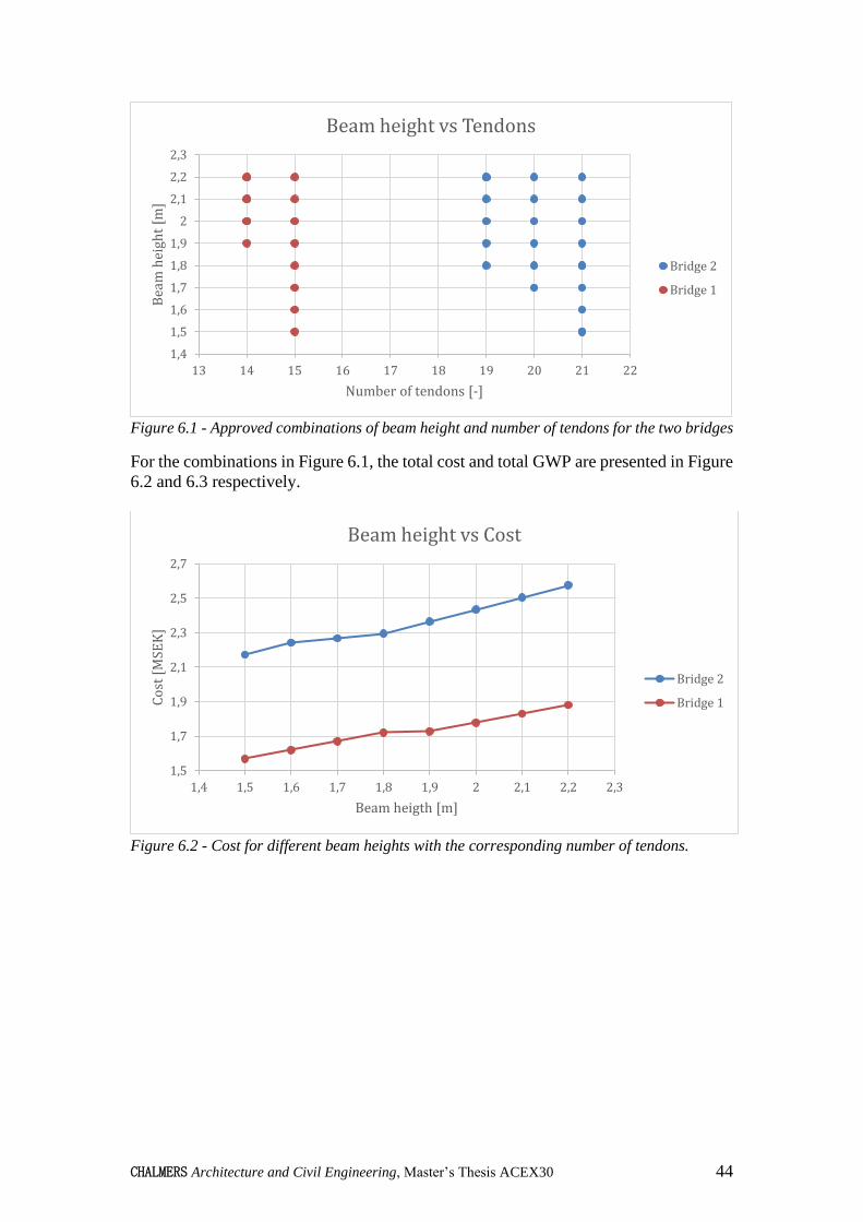
CHALMERS Architecture and Civil Engineering, Master’s Thesis ACEX30 44
Figure 6.1 - Approved combinations of beam height and number of tendons for the two bridges
For the combinations in Figure 6.1, the total cost and total GWP are presented in Figure
6.2 and 6.3 respectively.
Figure 6.2 - Cost for different beam heights with the corresponding number of tendons.
1,4
1,5
1,6
1,7
1,8
1,9
2
2,1
2,2
2,3
13 14 15 16 17 18 19 20 21 22
Bea
m h
eigh
t [m
]
Number of tendons [-]
Beam height vs Tendons
Bridge 2
Bridge 1
1,5
1,7
1,9
2,1
2,3
2,5
2,7
1,4 1,5 1,6 1,7 1,8 1,9 2 2,1 2,2 2,3
Co
st [
MSE
K]
Beam heigth [m]
Beam height vs Cost
Bridge 2
Bridge 1

CHALMERS Architecture and Civil Engineering, Master’s Thesis ACEX30 45
Figure 6.3 - GWP for different beam heights with the corresponding number of tendons.
6.2 Minimum beam height for different span lengths
To see the development of minimum beam height needed over different span lengths,
and the effect of the tendon layout parameters, the two bridges presented in Table 6.2
are evaluated by varying their span lengths in the range of 28 m – 38 m. The lowest
beam height for each span length that fulfils the design checks are presented in Figure
6.4. In Table 6.3 the same solutions are stated for both bridges with the corresponding
number of tendons together with the resulting combination of the two parameters L0
and espan.
Figure 6.4 - Minimum beam height for different span lengths for the two bridges.
200 000
250 000
300 000
350 000
400 000
450 000
1,4 1,5 1,6 1,7 1,8 1,9 2 2,1 2,2 2,3
GW
P [
CO
2-e
q]
Beam heigth [m]
Beam height vs GWP
Bridge 2
Bridge 1
1,3
1,4
1,5
1,6
1,7
1,8
1,9
2
2,1
2,2
2,3
26 28 30 32 34 36 38 40
Bea
m h
eigh
t [m
]
Span length [m]
Minimum beam height for different span lengths
Bridge 1
Bridge 2

CHALMERS Architecture and Civil Engineering, Master’s Thesis ACEX30 46
Table 6.3 - Minimum beam height for different span lengths with the corresponding number of
tendons, L0 and espan parameters.
Span
length
Beam
height
Number of
tendons L0 span*
Width 8m
28m 1.6m 13 0.75 * Lspan 20 %
30m 1.5m 15 0.75 * Lspan 20 %
32m 1.7m 14 0.85 * Lspan 20 %
34m 1.8m 15 0.85 * Lspan 10 %
36m 1.8m 15 0.85 * Lspan 0 %
38m >2.3m - - -
Width 11m
28m 1.5m 18 0.75 * Lspan 20 %
30m 1.4m 21 0.75 * Lspan 20 %
32m 1.4m 20 0.85 * Lspan 20 %
34m 1.5m 21 0.85 * Lspan 10 % / 20 %
36m 1.6m 21 0.85 * Lspan 0 %
38m 2.2m 21 0.85 * Lspan 0 %
* espan = LCG – (200mm + span * LCG)
6.3 Effect of chosen beam width and maximum number of
tendons
The width of the beam is chosen as input data and is set to half the width of the bridge
as a standard value. The web width sets the limit for the maximum number of tendons
and the results in Section 6.1 show that an increased number of tendons and a reduced
concrete cross-section is preferable. Therefore, a comparison of three different
combinations of web width and the maximum number of tendons is performed with the
standardized 8 m wide bridge from Section 6.1. The two new bridges will have the same
input except one will have a reduced ccduct distance to allow more tendons while the
last bridge will have the same number of tendons, i.e., 15, but the web width is
decreased by 0.5 m. The minimum concrete distance between the tendons is the
diameter of the duct (SIS, 2005a), so the minimum centre to centre distance is twice the
diameter which for this comparison is 190 mm. The input that differs between the
bridges are presented in Table 6.4 and the remaining input is the same as presented in
Table 6.1.
Table 6.4 – Differences of the input for the bridges compared in Section 6.3.
Bridge 1 Bridge 2 Bridge 3
Width [m] 8 8 8
Web width [m] 4 4 3.5
Max ccduct [m] 0.25 0.19 0.22
Max number of tendons 15 19 15

CHALMERS Architecture and Civil Engineering, Master’s Thesis ACEX30 47
The bridges are evaluated for different spans ranging from 28 m to 38 m where only
the lowest beam height that fulfils the criteria is presented. This is most likely the most
cost and environmentally efficient as described above. The set h is set to have an
interval of 100 mm ranging from 1.3 m to 2.3 m. Figure 6.5 shows the lowest beam
height needed and its corresponding number of tendons for different span lengths for
each of the bridges in Table 6.4.
Figure 6.5 - Minimum beam height for different span lengths for the different input data for the
bridge design.
In Figure 6.6 and Figure 6.7 the cost and GWP are presented for the bridges
respectively.
1
1,2
1,4
1,6
1,8
2
2,2
2,4
25 27 29 31 33 35 37 39
Bea
m h
eigh
t [m
]
Span length [m]
Beam height for different span lenghts
Bridge 1 Bridge 2 Bridge 3

CHALMERS Architecture and Civil Engineering, Master’s Thesis ACEX30 48
Figure 6.6 - Cost comparison of different input data for the bridge design.
Figure 6.7 - Comparison of GWP for different input data for the bridge design.
1,2
1,4
1,6
1,8
2
2,2
2,4
25 27 29 31 33 35 37 39
Co
st [
MSE
K]
Span length [m]
Cost of bridge for different span lenghts
Bridge 1 Bridge 2 Bridge 3
160 000
200 000
240 000
280 000
320 000
360 000
400 000
27 29 31 33 35 37 39
GW
P [
CO
2-e
q]
Span length [m]
GWP for different span lenghts
Bridge 1 Bridge 2 Bridge 3

CHALMERS Architecture and Civil Engineering, Master’s Thesis ACEX30 49
6.4 Comparison to existing bridges
To evaluate the potential of the optimization method implemented in the created python
tool, comparisons of the optimized solutions with two existing bridges designed by
Inhouse Tech Göteborg AB is performed.
6.4.1 Bridge 100-411-1
The first bridge to be compared has two equal spans of 32m each and a width of 11m.
Table 6.5 contains detailed information about both the existing bridge and the optimized
bridge.
Table 6.5 – Information about the two compared bridges.
Bridge Optimized Bridge 100-411-1
Span lengths [m] 32 32
Width [m] 11 11
Cross Section
Thickness top flange, tf [m] 0,30 0.29
Height, H [m] (1.3 - 2.0) 1.67
Web width, bw [m]
ccduct [m]
5.5
0.19
5.6
0.25
Wing walls and end-shields
Length of wing walls [m] 5.8 5.8
H2 [m] 1.1 1.1
Edge Beam
Width [m] 0.50 0.50
Height [m] 0.50 0.455
Materials
Concrete class C35/45 C35/45
Prestressing steel, fpk [MPa]
, Strand area [mm2]
, Number of strands per tendon [-]
1860
150
15
1860
150
15
Tendon layout
espan [mm] (e1, e2, e3 e4, e5)* 710
L0 [m]
Number of tendons
(24.0, 25.6, 27.2)
(0-27)
27.0
19
*Dependent on beam height.
Figure 6.8 displays the combinations of beam height and the minimum number of
tendons that fulfil the checks for each beam height in the set h. The set h contains beam
heights with an interval of 100 mm ranging from 1.3 m to 2.0 m for the optimized
bridge. The existing bridge is also displayed for comparison.
The lowest beam height that did work was 1.4 m with 22 tendons. Designs with 23-27
tendons were generated, but the beam height was not decreased for any of them. These
results are excluded from Figure 6.8-6.10 since more tendons for the same beam height
only uses more material and therefore will not be a better solution.

CHALMERS Architecture and Civil Engineering, Master’s Thesis ACEX30 50
Figure 6.8 - Number of tendons needed for different beam heights compared with existing
bridge.
For the combinations in Figure 6.8, the total cost and total GWP are presented in Figure
6.9 and 6.10 respectively for both bridges.
Figure 6.9 - Cost for different beam heights with the corresponding number of tendons
compared with the existing bridge.
1,3
1,4
1,5
1,6
1,7
1,8
1,9
2
2,1
17 18 19 20 21 22 23
Bea
m h
eigh
t [m
]
Number of tendons [-]
Beam height vs Number of tendons
2
2,05
2,1
2,15
2,2
2,25
2,3
2,35
2,4
2,45
1,3 1,4 1,5 1,6 1,7 1,8 1,9 2 2,1
Co
st [
MSE
K]
Beam height[m]
Beam height vs Cost
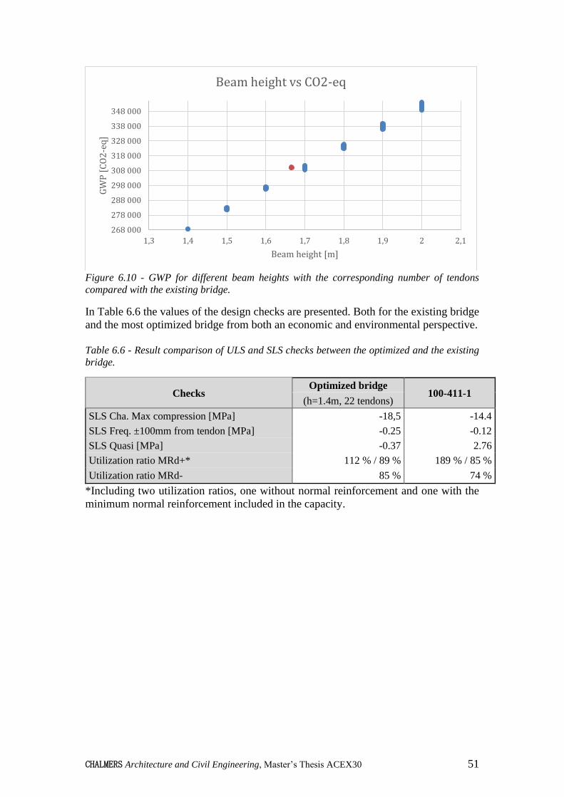
CHALMERS Architecture and Civil Engineering, Master’s Thesis ACEX30 51
Figure 6.10 - GWP for different beam heights with the corresponding number of tendons
compared with the existing bridge.
In Table 6.6 the values of the design checks are presented. Both for the existing bridge
and the most optimized bridge from both an economic and environmental perspective.
Table 6.6 - Result comparison of ULS and SLS checks between the optimized and the existing
bridge.
Checks Optimized bridge
100-411-1 (h=1.4m, 22 tendons)
SLS Cha. Max compression [MPa] -18,5 -14.4
SLS Freq. ±100mm from tendon [MPa] -0.25 -0.12
SLS Quasi [MPa] -0.37 2.76
Utilization ratio MRd+* 112 % / 89 % 189 % / 85 %
Utilization ratio MRd- 85 % 74 %
*Including two utilization ratios, one without normal reinforcement and one with the
minimum normal reinforcement included in the capacity.
268 000
278 000
288 000
298 000
308 000
318 000
328 000
338 000
348 000
1,3 1,4 1,5 1,6 1,7 1,8 1,9 2 2,1
GW
P [
CO
2-e
q]
Beam height [m]
Beam height vs CO2-eq

CHALMERS Architecture and Civil Engineering, Master’s Thesis ACEX30 52
6.4.2 Bridge 100-412-1
The second bridge to be compared has two equal spans of 36.8 m each and a width of
8 m. Table 6.7 contains detailed information about both the existing bridge and the
optimized bridge.
Table 6.7 – Information about the two compared bridges.
Bridge
Optimized
Bridge 1
Optimized
Bridge 2
100-412-1
Span lengths [m] 36.8 36.8 36.8
Width [m] 8 8 8
Cross Section
Thickness top flange, tf [m] 0.30 0.30 0.275
Height, H [m] (1.3 - 2.3) (1.3 - 2.3) 1.9
Web width, bw [m]
ccduct [m]
4
0.2
3.44
0.19
3.4
0.18
Wing walls and end-shields
Length of wing walls [m] 5.8 5.8 5.8
H2 [m] 1.1 1.1 1.1
Edge Beam
Width [m] 0.50 0.50 0.50
Height [m] 0.50 0.50 0.455
Materials
Concrete class C35/45 C35/45 C35/45
Prestressing steel, fpk [MPa]
, Strand area [mm2]
, Number of strands per
tendon [-]
1860
150
15
1860
150
15
1860
150
15
Tendon layout
espan [mm] (e1, e2, e3 e4, e5)* (e1, e2, e3 e4, e5)* 876
L0 [m]
Number of tendons
(27.6, 29.4, 31.3)
(0-19)
(27.6, 29.4, 31.3)
(0-17)
31.2
17
*Dependent on beam height.
Figure 6.11 displays the combinations of beam height and the minimum number of
tendons that fulfil the design checks for each beam height in the set h. The set h will
contain beam heights with an interval of 100mm ranging from 1.3m to 2.3m for the
optimized bridge. The existing bridge is also displayed for a comparison.

CHALMERS Architecture and Civil Engineering, Master’s Thesis ACEX30 53
Figure 6.11 - Number of tendons needed for different beam heights compared with existing
bridge.
For the combinations in Figure 6.11, the total cost and total GWP are presented in
Figure 6.12 and 6.13 respectively for both bridges.
Figure 6.12 - Cost for different beam heights with the corresponding number of tendons
compared with the existing bridge.
1,5
1,6
1,7
1,8
1,9
2
2,1
2,2
2,3
2,4
14 15 16 17 18 19 20
Bea
m h
eigh
t [m
]
Number of tendons [-]
Beam height vs Number of tendons
Width 4m
Width 3,44m
100-412-1
1,8
1,85
1,9
1,95
2
2,05
2,1
2,15
2,2
1,5 1,7 1,9 2,1 2,3 2,5
Co
st [
MSE
K]
Beam height [m]
Beam height vs Cost
Width 4m
Width 3,44m
100-412-1

CHALMERS Architecture and Civil Engineering, Master’s Thesis ACEX30 54
Figure 6.13 - GWP for different beam heights with the corresponding number of tendons
compared with the existing bridge.
In Table 6.8 the values of the design checks are presented. Both for the existing bridge
and the most optimized bridge from an economical perspective.
Table 6.8 - Result comparison of ULS and SLS checks between the optimized and the existing
bridge.
Checks Optimized bridge
100-412-1 (h=1.8m, 17 tendons)
SLS Cha. Max compression [MPa] -14.9 -15.65
SLS Freq. ±100mm from tendon [MPa] -0.48 -0.03
SLS Quasi [MPa] 1.44 2.89
Utilization ratio MRd+* 147 % / 97 % 79%
Utilization ratio MRd- 81 % 77 %
*Including two utilization ratios, one without normal reinforcement and one with the
minimum normal reinforcement included in the capacity.
Table 6.9 shows a summarize of the reduction concerning both cost and GWP for the
optimized solutions compared to the existing bridges 100-411-1 and 100-412-1.
Table 6.9 – Summarization of the reduction for the cost and GWP compared to the existing
bridge designs.
100-411-1 100-412-1
Reduction of cost 4.1 % 3.0 %
Reduction of CO2 - equivalent 13.4% 5.1%
220 000
230 000
240 000
250 000
260 000
270 000
280 000
1,5 1,7 1,9 2,1 2,3 2,5
GW
P [
CO
2-e
q]
Beam height [m]
Beam height vs CO2-eq
Width 4m
Width 3,44m
100-412-1

CHALMERS Architecture and Civil Engineering, Master’s Thesis ACEX30 55
7 Discussion
The part of the results which aims to simulate and show different patterns regarding the
relation between the design solutions and their cost and global warming potential is
discussed in Section 7.1. The comparison between the optimised design and the
previous design of two existing bridges is treated in the following Section 7.2. Some
simplifications have been made in the study and how these can affect the result is
explained in Section 7.3.
7.1 General Results
The result in Section 6.1 shows that the smallest beam heights with a large number of
tendons are the best solutions from both economic and environmental point of view.
However, figure 6.2 shows that there can be cases where this is not true, and that this
is the case for the narrower bridge geometry, denoted Bridge 1. Here, one tendon could
be taken away when increasing the beam height from 1.8 m to 1.9 m and these two
designs has an equal cost. The larger concrete cross-section could lead to that the
amount of normal reinforcement can be decreased. A larger cross-section generally also
requires less shear reinforcement and a decrease in construction hours on site. On the
other hand, the higher beam had larger GWP and was thus worse from an environmental
point of view. Consequently, the smaller beam height may be considered as a better
solution anyway.
A general pattern that was noticed is the importance of the tendon layout to balance the
positive and the negative effects from the prestressing in the design of the cross-section.
This is of special importance for the shorter spans, where the secondary moment creates
a positive moment over the mid support as described in Section 2.1.3, and the positive
moment capacity is rather small due to that the tendons are placed at the top of the
beam. This positive moment needs then to be counteracted with the negative moment
from the self-weight, but the load effect from the self-weight is rather small due to the
short spans. For the same reason, this is of less importance for spans of 34 m and longer,
where the negative moment from the self-weight is larger than the secondary moment.
For the longer spans, the maximum compression stress in the concrete at the top of the
cross-section can be decisive and limit how many tendons can be used.
To get the most optimal solution, especially for the short spans, the set of the parameters
L0 and espan, described in Section 4.1, that influences the tendon layout should be
modified. The sets should include more values with smaller intervals to find this
balance between the positive and negative effect of the prestressing. This takes a lot of
computational power and time, which is why a larger set was not used in this study.
The sets could also be modified depending on span lengths. From Table 6.3 it can be
seen that there is a correlation between span lengths and the variables for the tendon
layout. For the shorter spans, 28 m and 30 m, the most optimal solutions had L0 equal
to 75 % of the span length and a high position of the cable in the span (i.e., when αspan
is 20 %). For the medium-length spans, the value on L0 changes to 85 % but the cable
remains high in the span, and for the longer spans the position of the cable is changed
so that it has the lowest placements possible in the span. With this knowledge, the set
for L0 could be changed so that it, for example, contains more values closer to 75 % and

CHALMERS Architecture and Civil Engineering, Master’s Thesis ACEX30 56
skip 85 % if the spans that are studied is around 28-30 m. Since only these two values
on L0 have been used for the general results, the increase of L0 between 75 % and 85 %
might not be the most optimal values for the intermediate span lengths. For bridge 100-
411-1 with a span of 32 m, the most optimized solution has L0 at 80 % which makes it
reasonable to assume that the most optimal value for L0 has a linear pattern for the spans
between 28 and 38 m.
In Section 6.3 it can be seen that even more optimized bridges can be obtained by
increasing the number of tendons and by reducing the beam width. When the span
lengths are above 32 m both the increased maximum number of tendons and the
decreased width of the beam gives more optimal bridges than the original input. If the
economical aspect is of priority, the decreased beam width (Bridge 3) gives the most
optimal bridge. Figure 6.5 shows that the beam height is almost the same for Bridge 1
and 3, and since the number of tendons is the same for the two bridges, the only thing
that differs is the amount of concrete due to the different beam widths. For span lengths
above 32 m, it is rather clear that the concrete which adds self-weight to the structure
is not needed and can be taken away to reduce both the cost and GWP. However, for
Bridge 3 with spans of 28-30 m, the self-weight is needed to counteract the secondary
moment, and therefore the reduced web width only has negative effects and there are
no solutions found that fulfils the design requirements.
The increased number of tendons with the standard beam width (Bridge 2) gives the
best results concerning the GWP for the span lengths of 32 m and longer, which can be
seen in Figure 6.7. This is due to that the increased number of tendons allows for a
lower beam height. The decreased beam height results in that the amount of concrete
could be decreased even more than when the beam width is reduced (Bridge 3). The
increased number of tendons makes the solution more expensive than reducing the
beam width, but since the GWP is very much connected to the amount of concrete used,
this solution is to prefer.
As can be seen in Figure 6.4 and in Section 6.3, the optimal beam height increases for
28 m span length compared to 30 m span length. This is due to that the load effect from
the self-weight is rather small compared to the secondary moment from the prestressing
steel. This leads to that the number of tendons needs to be reduced to lower the effect
of the secondary moment and, consequently, the height of the beam then needs to be
increased to have enough capacity. This is a case where the tendon layout is of high
importance if a lower beam height is wanted. To obtain a lower beam height, the tendon
layout would need to be modified such that the secondary moment is reduced even more
than allowed with the sets chosen in this study. However, this would probably lead to
that more tendons are needed and therefore may not be the most optimal solution
anyway.
7.2 Comparison to two existing bridges
Bridge 100-411-1
For bridge 100-411-1, with two spans of 32 m, the comparison shows that there are
design solutions where the height of the beam could be decreased if more tendons are
added. The optimization shows three cheaper design solution and six design solutions
with lower GWP. The optimized bridge, presented in Table 6.6, has a decreased cost of

CHALMERS Architecture and Civil Engineering, Master’s Thesis ACEX30 57
4.1% compared to the existing bridge. The largest improvement is on the GWP, where
the optimized bridge has a 13.4% smaller GWP. This is achieved through decreased
beam height and smaller amount of concrete needed, which has a strong influence on
the GWP.
For the most optimal design solution, with a beam height of 1.4 m and 22 tendons, the
maximum compression stress under Quasi-permanent loading is 0.37 MPa. The
existing bridge has large tensile stress under Quasi-permanent loading (2.76 MPa)
which requires a crack width check to be performed. For the optimized bridge, no extra
crack width check needs to be performed since the entire beam cross-section is under
compression, which is desirable in the design. The design solution which has almost
the same beam height as the existing solution, but one more cable, has smaller tensile
stress than the existing bridge for the same load case (0.76 MPa). The maximum tension
stresses are in the bottom of the beam over the support, which is caused by the
secondary moment. So, the difference between the existing bridge and the optimized
designs is that the optimized solution has a tendon layout which decreases the secondary
moment more compared to the existing bridge.
It can also be seen in Figure 6.8 that, for the same number of tendons as in the existing
bridge, the optimal design solution has 230 mm higher cross-section. Furthermore, for
about the same cross-section height, the optimal design solution has one more cable.
This shows that the positive moment capacity above the mid support is not enough for
the existing bridge without non-prestressed reinforcement for crack control. However,
for the existing bridge, this reinforcement was designed to handle the torsional moment.
Consequently, it could be used also for crack control in SLS. This crediting could be
used for the design of the bridge in a later design phase where the information about
the torsional reinforcement was available. For the early estimation, which the script is
supposed to be used for, this information is not available; the capacity is only crediting
the minimum reinforcement, which is the only amount of reinforcement that is known
to be provided in the beam at this stage. This leads to that the script does not accept the
design which is similar to the existing bridge, since the positive moment capacity is not
enough, and is instead searching for a design that fulfils all criteria. For this case, an
experienced engineer could study the results for the designs which fulfil all criteria
except the positive moment capacity at the mid support and do an estimation if the
design check is likely to be fulfilled in a later stage when more information is available.
Bridge 100-412-1
For bridge 100-412-2, with two spans of 36.8 m, the optimized bridge with a beam
width of 3.4 m. Here, there are both a design solution which has the same beam height
as the existing bridge but fewer tendons, and a solution with the same number of
tendons but lower beam height. These two designs are cheaper solutions than the
existing bridge. There are also two design solutions that have less GWP, where one of
them is a bridge with a 4 m wide beam, 19 tendons and 1.6 m beam height. This gives
the smallest cross-section of all designs for this comparison, which then gives the
lowest GWP. The most optimal solution is reducing the cost by 2.3 % and the GWP
with 4.5 %, which is considered good, but it could be stated that the existing design is
close to optimal regarding both cost and GWP. This result was expected based on two
important patterns discussed under Section 7.1. These are (1) that the number of tendons
should be maximized (set ccduct to 190 mm) and (2) for span lengths around 34 m and
above the web width can be decreased from the initial 50 % of the total width

CHALMERS Architecture and Civil Engineering, Master’s Thesis ACEX30 58
assumption. In the design of the existing bridge, both these conditions are implemented
and therefore it is relatively close to the optimized solution.
The optimized design shows good values for the SLS-checks compared to the existing
solution, which can be seen in Table 6.8. The stress under Quasi-permanent loading is
lower than for the existing bridge, which favours the crack width check that remains to
be made. It also has more margin in the stress check for Frequent loading, where the
existing bridge is very close to the limit. For the ULS-checks, the utilization ratio for
the optimized design is higher and the positive sectional moment is close to the
capacity. It is still a design that works and is less demanding with respect to the crack
width check. Consequently, it can be seen as a better design solution than the existing
bridge since probably less non-prestressed reinforcement is needed to avoid too large
crack widths.
7.3 Simplifications
The optimization process for this study is only taking the prestressing steel and the
dimensions of the cross-section into account with respect to its capacity in bending.
This results in that the design which is determined to be cheapest or to have the smallest
GWP is also only considering these two parameters. A very slim solution may then
become the best solution according to this study, but it may also lead to the need for
more shear and non-prestressed reinforcement in the beam, something that will lead to
an increase of the cost and GWP.
Since no crack width control is included in the analysis, this is something that needs to
be designed for later in the design process. To avoid the need to perform this later, a
check to analyse if the whole beam is in compression under quasi-permanent loading
could have been added to the optimization loop. When this was included, several design
solutions did not fulfil this criterion and were therefore not considered to be acceptable
solutions. This resulted in that the final design solutions gave considerably higher cost
and GWP than the ones that did not include the crack check. Therefore, the decision
was taken not to include the crack width check in the optimization algorithm to allow
more slim solutions and accept that a crack width check must be done later in the design
process. This may then lead to increased amounts of non-prestressed reinforcement.
The stresses in the beam under quasi-permanent loading is although included in the
output from the optimization tool, together with the results from the analysis for post-
processing.
This could potentially result in that a solution that is accepted by the optimisation tool
is not possible to use, if the crack width criteria cannot be fulfilled. However, this is not
expected to be a common case since other checks are usually not fulfilled if the beam
shows this behaviour with large tensile stresses under quasi-permanent loading. This
include, for example, the check in SLS that the concrete is in compression 100 mm over
and under the cable, and the check of the positive moment capacity over the support in
ULS. Furthermore, the structural engineer that is using this optimization method could
easily implement an upper limit on the allowed tensile stress under quasi-permanent
loading. This upper limit could then be determined from experience to a value that give
good solutions with respect to the crack width check.

CHALMERS Architecture and Civil Engineering, Master’s Thesis ACEX30 59
8 Conclusion
In this master’s thesis, a tool was developed for optimization of two-span continuous
prestressed concrete beam bridges, suitable for early design stages. When comparing to
two newly designed existing bridges, the optimization tool designed more material-
efficient solutions, especially for one of the bridges where the GWP was reduced by 13
%. It was shown that a slim bridge design with a high number of tendons is preferable
compared to an increased beam height with fewer tendons when considering both
economy and GWP.
To obtain the most optimized design solutions using the tool, the distance between the
ducts should be minimized to allow the maximum number of tendons possible and
iterate different design solutions. The iterative process should be continued until the
lowest beam height with a corresponding number of tendons is reached. The web width
should be chosen to approximate 50 % of the bridge width for spans equal to or lower
than 32 m, while for longer spans it can be reduced. In this thesis, it has been reduced
to 43% of the total width which resulted in a good design from both an economic and
environmental point of view. However, a more slim cross-section leads to an increased
amount of shear and non-prestressed reinforcement, something that is not studied in
this thesis.
It is important to find a good balance between the positive effect of the longitudinal
compression from the tendons and the negative effect of the secondary moment they
are causing. This is of most importance for spans of 32 m or shorter, and therefore the
tendon layout is an important factor to handle for the optimization to work successfully.
For these shorter span lengths, it is important that the tendon layout leads to a small
secondary moment. Since the moment from the self-weight is smaller for shorter spans
the secondary moment has a larger effect on the bridge design. In the tool developed,
this was done by modifying the two sets for the parameters that affect the tendon layout,
L0 and espan, such that the lowest point of the tendon in the span has a higher position
and that the tendon intersects with the beam’s centre of gravity further away from the
mid support. With a good layout of the tendons, the number of tendons could be
increased, and the concrete cross-section decreased.
More optimal design solutions were found using the optimization tool, compared to the
experience-based design solutions used for the existing bridges studied. Consequently,
it can be concluded to be beneficial and relevant to use such a tool in the preliminary
design phase. The results show that the set-based parametric design (SBPD) method
can be used to find an optimized combination between a tendon layout, number of
tendons and beam height for each specific bridge design. More conclusions can be
drawn for each bridge geometry by using the optimization tool, but it is hard to
generalise these into simple design recommendations for early design stages. Instead,
the most optimal solution is changing from case to case. However, the optimization tool
with the implemented SBPD-method is generating a low-cost design that is
environmentally friendly with a slim cross-section together with a high number of
tendons.

CHALMERS Architecture and Civil Engineering, Master’s Thesis ACEX30 60
8.1 Further investigations
In this thesis, the model and analysis have been limited to only include the basic layout
of the structure, which is often enough for estimations in the early design phase. The
tool could be extended in several ways to include more parts of the bridge design.
The design of non-prestressed reinforcement could be included, which would give an
even more accurate optimization concerning economy and GWP due to that a slim
design often results in more non-prestressed reinforcement to reach enough shear and
torsion capacity. An increased amount of reinforcement would also lead to an additional
increase in cost due to more labour work on site.
When analysing different bridge designs, the effect of a changed tendon layout has been
found to have a large impact on the optimization results. Therefore, it could be of
interest to further investigate this to develop and implement a larger and more advanced
optimization of the tendon layout in the tool. This could be performed in two different
ways: If a new optimization study regarding the tendon layout results in a general
conclusions regarding optimal tendon design, these could easily be implemented in the
tool. However, as discussed in Chapter 7, the most optimal values of the two parameters
espan and L0 depends on the bridge geometry, and the most optimal values on the two
parameters can change. Therefore, a further investigation in the choice of these two sets
could lead to that more accurate values can be chosen for the sets, which would likely
result in an even more optimized bridge design.
As mentioned in the discussion, the SBPD method used in this optimisation tool shows
good results and could most likely be implemented in more design phases for other
bridge types, or other geometries with good results. A fairly large amount of re-coding
of the developed python-script would be necessary, however the structure and layout
of the tool could be used in the future for other optimization tools.

CHALMERS Architecture and Civil Engineering, Master’s Thesis ACEX30 61
9 References
Boverket. (2021). Utsläpp av växthusgaser från bygg- och fastighetssektorn.
Https://Www.Boverket.Se/Sv/Byggande/Hallbart-Byggande-Och-
Forvaltning/Miljoindikatorer---Aktuell-Status/Vaxthusgaser/.
Dolan, C. W., & Hamilton, H. R. (2019). Prestressed Concrete : Building, Design, and
Construction. Springer Nature Switzerland. https://doi.org/10.1007/978-3-319-
97882-6
Engström, B. (2011a). Design and analysis of deep beams, plates and other
discontinuity regions. 55.
Engström, B. (2011b). Design and analysis of prestressed concrete structures.
Fu, F. (2018). Design and Analysis of Tall and Complex Structures (Issue 2018).
Elsevier Science and Techonology. ProQuest Ebook Central,
https://ebookcentral.proquest.com/lib/chalmers/detail.action?docID=5257306.
Gosavi, A. (2015). Simulation-Based Optimization - Parametric Optimization
Techniques and Reinforcement Learning (2nd ed.). Springer Scince+Business
Media. https://doi.org/10.1002/9781119019770.ch13
Naturvårdsverket. (n.d.). Koldioxidekvivalenter. Retrieved March 12, 2021, from
https://www.naturvardsverket.se/Sa-mar-miljon/Statistik-A-O/Vaxthusgaser-
konsumtionsbaserade-utslapp-fran-exporterande-foretag/Koldioxidekvivalenter/
Naturvårdsverket. (2020). Bygg- och fastighetssektorns klimatpåverkan.
Https://Www.Naturvardsverket.Se/Sa-Mar-Miljon/Klimat-Och-Luft/Klimat/Tre-
Satt-Att-Berakna-Klimatpaverkande-Utslapp/Bygg--Och-Fastighetssektorns-
Klimatpaverkan/.
Pacoste, C., Plos, M., & Johansson, M. (2012). Recommendations for finite element
analysis for the design of reinforced concrete slabs. KTH.
Rempling, R., Mathern, A., Tarazona Ramos, D., & Luis Fernández, S. (2019).
Automatic structural design by a set-based parametric design method. Automation
in Construction, 108, 102936. https://doi.org/10.1016/j.autcon.2019.102936
Rombach, G. A. (2004). Finite element design of concrete structures.
Scanscot Technology. (2015). Brigade Plus -User’s manual. 6.2.
Scanscot Technology. (2021). BRIGADE/Plus 6.2-20.
SIS. (2002a). Eurokod - Grundläggande dimensioneringsregler för bärverk.
SIS. (2002b). Eurokod 1: Laster på bärverk - Del 1-1: Allmänna laster - Tunghet,
egentyngd, nyttig last för byggnader. 08(121687).
SIS. (2003a). Eurokod 1 : Laster på bärverk – Del 2 : Trafiklast på broar. Svenska
institutet för standarder. Stockholm.
SIS. (2003b). Eurokod 1 – Laster på bärverk – Del 1-5 : Allmänna laster –
Temperaturpåverkan.
SIS. (2005a). Eurokod 2: Dimensionering av betongkonstruktioner - Del 1-1: Allmänna
regler och regler för byggnader. In Euro code SS-EN-1191-2 (Issue 138227).

CHALMERS Architecture and Civil Engineering, Master’s Thesis ACEX30 62
SIS. (2005b). Eurokod 2: Dimensionering av betongkonstruktioner - Del 2: Broar. In
Euro code SS-EN-1191-2.
Ström, M., Raudberget, D., & Gustafsson, G. (2016). Instant Set-based Design, an Easy
Path to Set-based Design. Procedia CIRP, 50, 234–239.
https://doi.org/10.1016/j.procir.2016.04.194
Svensk Betong. (2017). Environmental product declaration - Betong för vägbro.
Trafikverket. (2019a). Bärighetsberäkning av broar - TDOK 2013:0267.
Trafikverket. (2019b). Krav Brobyggande. Trafikverket, 0–351.
http://trvdokument.trafikverket.se/Versioner.aspx?spid=289&dokumentId=TDO
K 2016%3A0204
Trafikverket. (2020). Klimatkalkyl (7.0).
Yavari, M. S., Pacoste, C., & Karoumi, R. (2016). Structural Optimization of Concrete
Slab Frame Bridges Considering Investment Cost. Journal of Civil Engineering
and Architecture, 10(9), 982–994. https://doi.org/10.17265/1934-
7359/2016.09.002

Appendix A
Hand calculations
EI N m2
:=
Geometry
l1 32m:=
l2 32m:=
l3 1.3m:=
h 2m:= Height if beam
b 7.8m:= Width of top flange in T-section
bw 4m:= Width of web
tf 0.55m:= Thickness of top flange
hw h tf- 1.45m=:= Height of web
Ac tf b hw bw+ 10.09m2
=:= Cross section area
xTP
bw
hw2
2 b tf hw
tf
2+
+
Ac1.15m=:= Distance from bottom to centre of gravity
Ibw hw
3
12bw hw
hw2
2+
b tf3
12+ b tf hw
tf
2+
2
+ 19.987m4
=:= Moment of intertia

Ec 34GPa:= Modulus of elasticity for concrete
EI Ec I 6.796 1011
m3kg
s2
=:=
tpaving 100mm:= Thickness of paving
tww 0.5m:= Thickness of wingwall
tendscreen 0.6m:= Thickness of endshield
hendscreen 4m:= Height of end-shield
Vendscreen tendscreen b hendscreen 18.72 m3
=:=
Vww hendscreen 1.1 m4.7m( )
2
2+
tww 7.723 m
3=:=
Loads
ρc 25kN
m3( )
:= Density of concrete
ρpaving 23kN
m3
:= Density of paving
qd Ac ρc tpaving b ρpaving+ 270.19kN
m=:= Evenly distributed self weight
Pww.es Vendscreen Vww+( ) ρc 661.063 kN=:= Point load at the end of the bridgedue to self weight of wingwall andend-shield
Condition: θ.B1 + θ.B2=0
θB1.qqd l1
3
24 EI:=Load :
θB2.qqd l2
3
24 EI:=

Support moment θB1.MMB- l1
3 EI:=
MB
θB2.MMB- l2
3 EI
MC- l2
6 EI+:=
MB
MC
qd l32
2Pww.es l3+ 1.088 10
3 kN m=:=
MB 1000kN m:=
MB rootqd l1
3
24 EI
qd l23
24 EI+
MB- l1
3 EI+
MB- l2
3 EI
MC- l2
6 EI2+
+ MB,
3.404 104
kN m=:=
MB 3.404 104
kN m=
RB2
qd l2
2
MB
l2+
MC
l2- 5.353 10
3 kN=:=
x0.2
RB2
qd19.811m=:=
M2.max
qd x0.22
2MB- 1.898 10
4 kN m=:=
MB
M2.max1.793=
Support moment comparison with BRIGADE Field moment comparison with BRIDGADE
M1.max.BRIGADE 1.906 104
kN m:=MB.BRIGADE 3.391 10
4 kN m:=
MB MB.BRIGADE-
MB0.383 %=
M2.max M1.max.BRIGADE-
M2.max0.408- %=

Appendix B
Project: 100-411-1Designer: JNtSystemberäkning, styv grundläggning
---------------------------------------------------------------------------BRIGADE/Standard version 4.3.23Project File Name: 100-411-1Model ID: 58327530Last save at: 2021-02-02 07:29:55Calculated with version: 4.3.23Last calc. started at: 2021-02-02 07:30:00Time: 2021-02-02 09:41:55---------------------------------------------------------------------------Result Set Name: Trafiklaster_Moment---------------------------------------------------------------------------Case 1: Classification vehicle a (no surface load), Max, Bending Moment Mh (kNm)Case 2: Classification vehicle a (no surface load), Min, Bending Moment Mh (kNm)Case 3: Classification vehicle b (no surface load), Max, Bending Moment Mh (kNm)Case 4: Classification vehicle b (no surface load), Min, Bending Moment Mh (kNm)Case 5: Classification vehicle c (no surface load), Max, Bending Moment Mh (kNm)Case 6: Classification vehicle c (no surface load), Min, Bending Moment Mh (kNm)Case 7: Classification vehicle d (no surface load), Max, Bending Moment Mh (kNm)Case 8: Classification vehicle d (no surface load), Min, Bending Moment Mh (kNm)Case 9: Classification vehicle e (no surface load), Max, Bending Moment Mh (kNm)Case 10: Classification vehicle e (no surface load), Min, Bending Moment Mh (kNm)Case 11: Classification vehicle f (no surface load), Max, Bending Moment Mh (kNm)Case 12: Classification vehicle f (no surface load), Min, Bending Moment Mh (kNm)Case 13: Classification vehicle g (no surface load), Max, Bending Moment Mh (kNm)Case 14: Classification vehicle g (no surface load), Min, Bending Moment Mh (kNm)Case 15: Classification vehicle h (no surface load), Max, Bending Moment Mh (kNm)Case 16: Classification vehicle h (no surface load), Min, Bending Moment Mh (kNm)Case 17: Classification vehicle i (no surface load), Max, Bending Moment Mh (kNm)Case 18: Classification vehicle i (no surface load), Min, Bending Moment Mh (kNm)Case 19: Classification vehicle j (no surface load), Max, Bending Moment Mh (kNm)Case 20: Classification vehicle j (no surface load), Min, Bending Moment Mh (kNm)Case 21: Classification vehicle k (no surface load), Max, Bending Moment Mh (kNm)Case 22: Classification vehicle k (no surface load), Min, Bending Moment Mh (kNm)Case 23: Classification vehicle l (no surface load), Max, Bending Moment Mh (kNm)Case 24: Classification vehicle l (no surface load), Min, Bending Moment Mh (kNm)Case 25: Classification vehicle m (no surface load), Max, Bending Moment Mh (kNm)Case 26: Classification vehicle m (no surface load), Min, Bending Moment Mh (kNm)Case 27: Classification vehicle n (no surface load), Max, Bending Moment Mh (kNm)Case 28: Classification vehicle n (no surface load), Min, Bending Moment Mh (kNm)Case 29: Traffic Load Model 1, TS, Max, Bending Moment Mh (kNm)Case 30: Traffic Load Model 1, TS, Min, Bending Moment Mh (kNm)
Appendix B
Page 1

Appendix B
Title Node Pos_ln Pos_tn Thickness Case1 Case2 Case3 Case42551 0 -0,07913 -1,244 -0,06938 -1,5212552 0,23 0,7507 -77,47 0,6953 -54,682553 0,45 1,606 -151,7 1,31 -104,72554 0,68 0,02804 -224,5 0,02417 -169,52555 0,9 0,4304 -297,2 0,3287 -253,72556 0,9 16,73 -297,1 12,35 -266,12557 1,21 0,1288 -397,3 0,152 -423,92558 1,53 0,04969 -497,5 0,0459 -582,52559 1,84 0,4918 -599,2 0,7209 -744,42560 2,15 1,252 -702,5 1,835 -909,72561 2,15 48,55 -700,6 50,5 -9082562 2,95 266,7 -716,4 397,7 -914,52563 3,75 474,6 -684,5 733,4 -875,22564 4,55 658,3 -650,5 1035 -835,22565 5,35 825,3 -614,3 1312 -792,72566 6,15 976,9 -576,7 1565 -748,72567 6,95 1110 -538,3 1793 -703,52568 7,75 1228 -499,2 1995 -657,62569 8,55 1334 -459,9 2176 -611,42570 9,35 1420 -420,8 2330 -565,42571 10,15 1491 -382,1 2462 -519,82572 10,95 1548 -343,9 2568 -474,92573 11,75 1601 -306,2 2658 -430,82574 12,55 1648 -269 2728 -416,32575 13,35 1681 -232,3 2780 -407,62576 14,15 1705 -195,8 2815 -399,22577 14,95 1719 -206,3 2839 -4252578 15,75 1718 -225,1 2849 -457,32579 16,55 1711 -243,9 2849 -489,72580 17,35 1694 -262,8 2831 -522,42581 18,15 1669 -283 2795 -556,42582 18,95 1645 -303,4 2745 -590,62583 19,75 1608 -323,8 2679 -6252584 20,55 1565 -344,5 2601 -6602585 21,35 1517 -365,5 2509 -695,42586 22,15 1460 -386,9 2416 -731,72587 22,95 1400 -408,8 2321 -768,82588 23,75 1334 -431,1 2208 -806,82589 24,55 1268 -453,9 2088 -845,62590 25,35 1203 -477 1963 -884,92591 26,15 1126 -500,2 1818 -924,42592 26,95 1053 -523,3 1676 -963,72593 27,75 976,3 -545,8 1531 -10022594 28,55 875,5 -558,5 1372 -10302595 29,35 772,1 -551,9 1186 -10382596 30,15 654,3 -526,7 981,9 -10262597 30,95 521,2 -484,3 759,6 -995,12598 31,75 365,5 -426,6 540,6 -948,22599 32,55 211,8 -355,8 311,7 -887,72600 33,35 167,5 -274,4 243,5 -817,12601 34,15 183,3 -184 266,4 -738,82602 34,15 183,1 -183,7 266,3 -738,62603 34,95 177,3 -279,1 243,9 -821,52604 35,75 211,2 -364,6 311,1 -896,2
Page 2

Appendix B
2605 36,55 364,2 -439,2 539,5 -960,62606 37,35 517,8 -500,2 756 -10112607 38,15 648,9 -545,5 975,5 -10442608 38,95 763,6 -572,6 1178 -10582609 39,75 862,5 -579,6 1359 -10512610 40,55 950,7 -564,5 1510 -10212611 41,35 1030 -544,7 1651 -984,92612 42,15 1101 -524,1 1793 -948,12613 42,95 1176 -503,4 1936 -9112614 43,75 1239 -482,7 2061 -874,22615 44,55 1299 -462,3 2175 -837,82616 45,35 1365 -442,4 2288 -802,32617 46,15 1427 -422,9 2386 -767,52618 46,95 1479 -404 2473 -733,72619 47,75 1527 -385,4 2559 -700,72620 48,55 1566 -367,3 2636 -668,32621 49,35 1597 -349,4 2697 -636,42622 50,15 1622 -331,6 2748 -604,82623 50,95 1644 -313,9 2779 -573,42624 51,75 1660 -296,4 2800 -542,12625 52,55 1668 -278,9 2802 -5112626 53,35 1662 -261,5 2785 -480,12627 54,15 1651 -244,3 2760 -449,42628 54,95 1624 -267,6 2723 -448,92629 55,75 1588 -304,6 2668 -458,22630 56,55 1545 -342,1 2601 -473,62631 57,35 1487 -380,1 2510 -518,62632 58,15 1425 -418,8 2397 -564,32633 58,95 1349 -458,1 2260 -610,92634 59,75 1260 -497,9 2104 -657,92635 60,55 1158 -537,9 1925 -705,22636 61,35 1035 -577,7 1718 -752,32637 62,15 899,8 -617,1 1489 -798,72638 62,95 748,7 -655,8 1235 -844,32639 63,75 580,3 -693,8 956,3 -888,92640 64,55 399 -730,7 657,3 -932,12641 65,35 201,3 -770,5 331,9 -979,52642 66,15 48,56 -808,3 47,98 -10272643 66,15 0,6337 -808 1,221 -10262644 66,46 0,2256 -681,1 0,4495 -8372645 66,78 0,04824 -556,3 0,07505 -6522646 67,09 0,05484 -433,3 0,07944 -470,22647 67,4 18,44 -309,8 13,47 -288,62648 67,4 0,2776 -310,6 0,2123 -275,32649 67,63 0,00643 -222,1 0,006781 -177,22650 67,85 0,4126 -132,4 0,3047 -97,152651 68,08 0,1979 -55,11 0,2777 -41,572652 68,3 9,053 -0,1056 8,344 -0,079
Page 3

Appendix B
Case5 Case6 Case7 Case8 Case9 Case10 Case11 Case12 Case13
-0,1981 -1,04 -0,1375 -1,145 -0,1514 -1,351 -0,2692 -0,9182 0,64970,6299 -62,93 0,6908 -70,14 0,6197 -47,38 0,5558 -54,12 0,6972
1,343 -122,4 1,473 -137 1,165 -89,93 1,183 -104,7 1,3120,02746 -180 0,03021 -202,3 0,02459 -145,4 0,02773 -153,3 0,04237
0,3708 -237,8 0,4079 -267,4 0,3007 -218,1 0,3365 -202 0,362914,04 -237,6 15,44 -267,4 10,96 -229,1 12,36 -201,9 12,36
0,1726 -331,3 0,1896 -357,1 0,1872 -377,3 0,2101 -281,2 0,41170,05216 -461,9 0,05737 -446,6 0,04554 -555 0,05136 -393 0,07721
0,818 -635,6 0,8984 -543,3 0,9576 -768,5 1,077 -544,4 2,3972,083 -828,2 2,286 -646,7 2,439 -998,9 2,742 -714,1 5,96341,34 -823,4 45,47 -677,3 45,48 -994,6 37,14 -736,2 34,81448,7 -833 489,1 -682,6 529,5 -996,8 582,9 -740,1 1092833,4 -796,5 912,1 -672,8 998,4 -954,2 1103 -730,2 21061181 -759,1 1294 -669,1 1426 -911,8 1579 -718,8 30101500 -719,2 1646 -663,2 1819 -866,8 2014 -705 38231791 -677,9 1966 -655,7 2175 -820 2410 -689,7 45552050 -635,5 2250 -647,1 2493 -772,1 2766 -673,2 51932281 -592,5 2501 -637,6 2774 -723,4 3082 -655,9 57392488 -553,5 2728 -627,4 3022 -677,8 3359 -640,6 61982665 -543,2 2920 -617,1 3234 -654,5 3599 -651,4 65742818 -533 3085 -606,8 3420 -631,5 3806 -662 68702946 -523,2 3223 -596,9 3579 -609 3980 -672,8 71233055 -513,8 3343 -587,6 3714 -587,2 4126 -684 73253140 -504,8 3434 -578,6 3823 -591,4 4245 -695,6 74623207 -496,3 3508 -570,2 3905 -601,1 4335 -707,7 75373255 -488,2 3559 -562,3 3965 -611,2 4401 -720,2 75533283 -517,7 3588 -593,5 4002 -651,1 4440 -764,1 75103291 -555,8 3602 -636,2 4010 -697,4 4455 -817,4 74123282 -594 3596 -679,1 4000 -743,9 4444 -870,9 72583254 -632,4 3566 -722,4 3965 -790,6 4411 -924,8 70543209 -672,2 3523 -767 3911 -838,9 4352 -980,2 69833152 -712,3 3457 -811,8 3846 -887,4 4269 -1036 70383080 -752,7 3374 -857,1 3759 -936,4 4168 -1092 70152997 -793,6 3278 -903 3657 -986 4050 -1149 69262899 -835,3 3168 -949,6 3537 -1036 3914 -1207 67682787 -877,8 3041 -997,3 3399 -1088 3758 -1266 65492663 -921,4 2899 -1046 3249 -1141 3588 -1327 62652528 -966 2752 -1096 3081 -1195 3402 -1389 59122380 -1012 2595 -1147 2900 -1250 3197 -1453 54952227 -1058 2421 -1199 2719 -1306 2973 -1517 50102071 -1104 2240 -1251 2521 -1363 2736 -1582 44551902 -1150 2044 -1303 2315 -1419 2495 -1647 38491723 -1195 1837 -1354 2093 -1474 2239 -1709 31791526 -1230 1613 -1393 1844 -1517 1958 -1761 26111301 -1244 1373 -1412 1576 -1540 1651 -1791 21721071 -1237 1111 -1410 1302 -1541 1320 -1799 1717
824,6 -1212 830,3 -1389 1005 -1523 984,4 -1787 1262563,9 -1169 536,4 -1350 693,7 -1487 635,1 -1757 807319,7 -1113 354 -1297 388,4 -1437 384,2 -1712 346,3278,5 -1047 307,7 -1235 296,8 -1378 299 -1659 338,8304,3 -976,7 335,9 -1175 319,1 -1313 317,7 -1606 361,4304,2 -976,5 335,8 -1175 319 -1313 317,6 -1605 361,3278,9 -1052 308,2 -1240 297,1 -1382 299,6 -1663 328,5327,5 -1122 362,7 -1306 394,3 -1446 387,9 -1721 358,3
Page 4

Appendix B
562,9 -1182 535,8 -1362 693,3 -1500 634,6 -1769 813,1821,7 -1227 827,7 -1404 1003 -1539 982 -1803 12811066 -1256 1106 -1429 1297 -1560 1315 -1818 17521291 -1264 1364 -1432 1569 -1560 1644 -1811 22231511 -1251 1602 -1414 1831 -1538 1949 -1782 26721703 -1214 1818 -1372 2069 -1492 2220 -1728 32041880 -1172 2022 -1324 2290 -1440 2473 -1667 38632046 -1128 2215 -1275 2496 -1387 2711 -1606 44532201 -1084 2396 -1225 2693 -1333 2948 -1543 49752353 -1040 2566 -1176 2872 -1279 3168 -1481 54402495 -997,1 2720 -1127 3046 -1226 3370 -1420 58472630 -954,9 2869 -1080 3215 -1174 3557 -1360 61962752 -913,7 3007 -1033 3367 -1124 3724 -1302 64772861 -873,6 3132 -987,8 3499 -1075 3876 -1245 66952960 -834,4 3244 -943,6 3620 -1027 4013 -1190 68453041 -796 3339 -900,3 3719 -979,6 4127 -1135 69293105 -758,2 3414 -857,6 3798 -933,2 4225 -1082 69433163 -720,7 3475 -815,3 3865 -887,3 4304 -1028 68913203 -683,4 3519 -773,2 3915 -841,6 4362 -975,6 70873234 -646,3 3542 -731,4 3951 -796,2 4394 -923,1 72933238 -609,5 3548 -689,8 3959 -751 4402 -870,9 74443227 -572,8 3535 -648,5 3945 -706,1 4387 -819,1 75363201 -536,4 3499 -607,5 3913 -661,5 4346 -767,6 75783150 -535,3 3451 -607,3 3849 -644,3 4276 -748,9 75553080 -544,4 3374 -616,1 3763 -635,3 4183 -737,4 74712994 -553,8 3278 -625,4 3657 -632,1 4063 -726,5 73282884 -563,9 3158 -635,3 3520 -654,8 3916 -716,1 71202751 -574,4 3017 -645,8 3356 -678,3 3739 -706,1 68442595 -585,4 2849 -656,8 3164 -702,4 3530 -696,5 65172414 -596,6 2653 -667,9 2949 -726,8 3286 -686,8 61242209 -636,6 2430 -678,8 2703 -773,7 3007 -703,3 56461975 -680,7 2174 -689,2 2418 -823,7 2690 -721,8 50881712 -724,2 1887 -698,9 2097 -873,1 2332 -739,6 44521422 -767 1567 -707,6 1740 -921,5 1935 -756,4 37221101 -808,8 1214 -715,4 1346 -968,7 1499 -772,3 2902
757 -849,4 835,5 -722,2 921,9 -1015 1026 -787,1 2004382,5 -893,6 422,8 -739,6 463,1 -1065 516,2 -804,7 102041,11 -938,3 45,36 -783,4 43,05 -1117 36,77 -851,9 11,511,471 -937,2 1,677 -755,6 1,829 -1116 2,137 -828,4 5,566
0,5448 -723,6 0,6232 -628,3 0,6808 -863,8 0,7981 -636,8 2,1690,08821 -528,4 0,09905 -509,2 0,1039 -628,4 0,1194 -463,8 0,24720,09666 -373,6 0,111 -396,7 0,1139 -426,6 0,1339 -328 0,3529
15,32 -257,6 16,88 -283,8 11,91 -255,5 13,45 -226,4 13,450,242 -258,4 0,2671 -284,5 0,1966 -243,7 0,2222 -227 0,2497
0,008342 -184,8 0,009646 -203,5 0,008516 -156,9 0,01016 -162,4 0,027460,3438 -110,4 0,3784 -121,3 0,2701 -86 0,302 -97,06 0,3030,1677 -46,02 0,1815 -50,49 0,2483 -36,92 0,1472 -40,44 0,2777
7,571 -0,08959 8,293 -0,09904 7,386 -0,07137 6,654 -0,08039 8,358
Page 5

Appendix B
Case14 Case15 Case16 Case17 Case18 Case19 Case20 Case21 Case22
-1,54 0,7842 -1,734 0,5802 -1,158 0,6678 -1,54 0,7842 -1,734-63,16 0,7896 -79,14 0,6925 -78,59 0,6978 -63,29 0,7896 -79,14-126,4 1,579 -158,8 1,478 -157,5 1,312 -126,4 1,581 -158,8-203,5 0,04355 -238,9 0,04294 -236,7 0,05122 -204,2 0,05578 -238,9-301,5 0,439 -344,8 0,4384 -315,7 0,3641 -302,6 0,4401 -344,8-313,9 15,38 -358,9 15,45 -315,6 12,36 -314,9 15,42 -358,9-490,8 0,3866 -561,1 0,4173 -439,1 0,4648 -492,3 0,4742 -561,1-668,9 0,07417 -764,7 0,07387 -604,8 0,08181 -670,7 0,08314 -764,7-857,3 2,214 -975,9 2,499 -821,2 2,402 -857,9 2,226 -975,9-1056 5,597 -1194 6,301 -1061 5,966 -1056 5,633 -1194-1092 47,76 -1230 35,6 -1071 31,6 -1090 47,76 -1230
-899 1054 -944,8 1089 -825,1 1086 -1065 1073 -1103-933,6 2037 -978,4 2097 -864,7 2082 -1092 2072 -1194-991,4 2928 -1012 3019 -921,4 2969 -1122 2980 -1288-1048 3756 -1043 3856 -975,8 3765 -1181 3823 -1381-1103 4506 -1071 4629 -1028 4482 -1277 4587 -1471-1156 5171 -1098 5338 -1079 5104 -1370 5264 -1559-1207 5753 -1124 6032 -1128 5633 -1461 5860 -1644-1257 6259 -1148 6656 -1175 6074 -1550 6378 -1727-1305 6692 -1176 7187 -1221 6453 -1637 6827 -1808-1353 7061 -1213 7637 -1311 6786 -1724 7208 -1889-1402 7362 -1296 8026 -1439 7046 -1810 7522 -1970-1451 7644 -1411 8351 -1568 7242 -1897 7777 -2051-1542 7874 -1527 8613 -1697 7370 -1985 7997 -2134-1660 8046 -1644 8804 -1827 7439 -2075 8161 -2218-1779 8164 -1761 8942 -1957 7449 -2165 8273 -2303-1898 8222 -1879 9023 -2089 7400 -2256 8325 -2389-2018 8224 -1998 9042 -2221 7296 -2348 8321 -2477-2140 8174 -2118 9047 -2355 7142 -2443 8274 -2566-2263 8078 -2239 9012 -2490 6951 -2538 8267 -2656-2386 8024 -2360 8915 -2625 6834 -2634 8206 -2747-2510 7915 -2482 8756 -2761 6893 -2730 8090 -2839-2635 7746 -2606 8538 -2899 6880 -2828 7920 -2932-2762 7528 -2731 8270 -3038 6798 -2928 7701 -3027-2891 7261 -2859 7948 -3181 6648 -3030 7431 -3124-3024 6941 -2990 7576 -3327 6438 -3136 7114 -3225-3160 6578 -3124 7155 -3476 6164 -3245 6753 -3329-3300 6159 -3262 6685 -3630 5828 -3357 6341 -3436-3442 5699 -3403 6173 -3787 5434 -3471 5887 -3547-3587 5194 -3546 5602 -3946 4972 -3588 5384 -3658-3732 4637 -3689 4978 -4105 4444 -3705 4835 -3771-3877 4041 -3832 4299 -4264 3853 -3821 4241 -3882-4019 3395 -3971 3576 -4420 3194 -3938 3599 -3992-4154 2705 -4105 2801 -4569 2474 -4184 2918 -4235-4279 1984 -4228 1981 -4707 1680 -4490 2195 -4629-4392 1572 -4340 1514 -4832 831,6 -4804 1435 -5071-4493 1231 -4439 1040 -4943 272,4 -5121 654,6 -5554-4652 883,9 -4527 568,5 -5041 298,3 -5439 292 -6063-5198 531,8 -4609 341,8 -5134 322,9 -5769 327,2 -6603-5779 411,8 -4695 380,5 -5231 347 -6115 361,8 -7189-6391 444,1 -4990 411,3 -5655 379,7 -6478 395,8 -7814-6388 443,9 -4988 411,1 -5653 379,5 -6476 395,7 -7811-5774 403,6 -4703 374,8 -5240 356,3 -6100 369,2 -7188-5193 492,1 -4619 330,1 -5145 332,6 -5757 342 -6605
Page 6

Appendix B
-4648 842,4 -4538 680,1 -5054 308,2 -5432 314,3 -6069-4502 1193 -4451 1092 -4957 282,5 -5114 597,4 -5564-4403 1607 -4353 1506 -4847 921,8 -4797 1370 -5087-4291 2006 -4243 1923 -4723 1779 -4483 2112 -4652-4167 2652 -4120 2739 -4586 2567 -4177 2831 -4268-4033 3340 -3987 3515 -4438 3274 -3931 3513 -4018-3892 3981 -3848 4246 -4284 3914 -3820 4153 -3901-3749 4573 -3707 4925 -4126 4488 -3712 4747 -3783-3605 5125 -3564 5549 -3968 5006 -3603 5296 -3665-3461 5635 -3422 6125 -3810 5464 -3494 5799 -3547-3320 6094 -3283 6644 -3654 5853 -3387 6251 -3430-3182 6511 -3146 7111 -3502 6182 -3282 6662 -3317-3047 6881 -3012 7525 -3353 6450 -3181 7026 -3207-2915 7204 -2883 7887 -3209 6656 -3083 7343 -3100-2787 7479 -2756 8197 -3068 6795 -2989 7612 -2997-2662 7706 -2631 8455 -2929 6869 -2897 7832 -2896-2538 7881 -2509 8660 -2793 6875 -2807 8002 -2797-2415 8007 -2388 8826 -2658 6810 -2718 8121 -2699-2293 8073 -2267 8968 -2524 6981 -2629 8181 -2602-2172 8127 -2147 9060 -2391 7181 -2542 8230 -2506-2052 8189 -2028 9089 -2258 7324 -2456 8287 -2410-1932 8197 -1910 9055 -2126 7415 -2370 8289 -2316-1813 8154 -1793 8963 -1996 7456 -2286 8238 -2223-1695 8051 -1676 8808 -1866 7431 -2202 8127 -2131-1617 7890 -1560 8599 -1736 7348 -2120 7961 -2040-1573 7674 -1444 8340 -1608 7208 -2039 7741 -1949-1531 7396 -1378 8036 -1490 7002 -1959 7465 -1860-1489 7087 -1362 7659 -1453 6745 -1881 7145 -1772-1447 6711 -1346 7203 -1415 6431 -1802 6763 -1684-1406 6266 -1331 6663 -1378 6041 -1722 6313 -1595-1363 5756 -1315 6036 -1339 5587 -1641 5798 -1504-1318 5165 -1297 5332 -1299 5045 -1558 5200 -1411-1272 4492 -1278 4608 -1257 4415 -1473 4527 -1316-1224 3734 -1257 3827 -1213 3694 -1384 3781 -1218-1173 2897 -1234 2981 -1167 2882 -1294 2949 -1119-1122 1999 -1209 2052 -1120 1988 -1202 2037 -1018-1073 1013 -1189 1038 -1076 1011 -1113 1031 -918,9-1051 57,19 -1216 35,63 -1089 12,22 -1061 49,09 -1216-1043 5,238 -1186 5,866 -1057 5,42 -1045 5,357 -1186
-842,7 2,007 -958,9 2,252 -804,4 2,112 -842,8 2,01 -959-652 0,2425 -742,2 0,2534 -582,2 0,2461 -652 0,2489 -742,1
-470,3 0,3243 -535,3 0,3553 -411,7 0,3956 -470,4 0,409 -535,4-289 16,88 -328,8 16,88 -284 13,54 -289,2 16,89 -329
-275,3 0,3006 -313,3 0,2981 -284,6 0,2487 -275,3 0,3012 -313,3-177,2 0,02543 -203,5 0,02665 -203,5 0,03417 -177,2 0,03624 -203,5-97,16 0,3779 -121,3 0,3796 -121,6 0,3037 -97,16 0,3795 -121,3-41,57 0,3167 -50,49 0,1854 -50,66 0,278 -41,57 0,3139 -50,49
-0,09183 9,508 -0,1093 8,335 -0,1073 8,368 -0,09835 9,52 -0,1184
Page 7
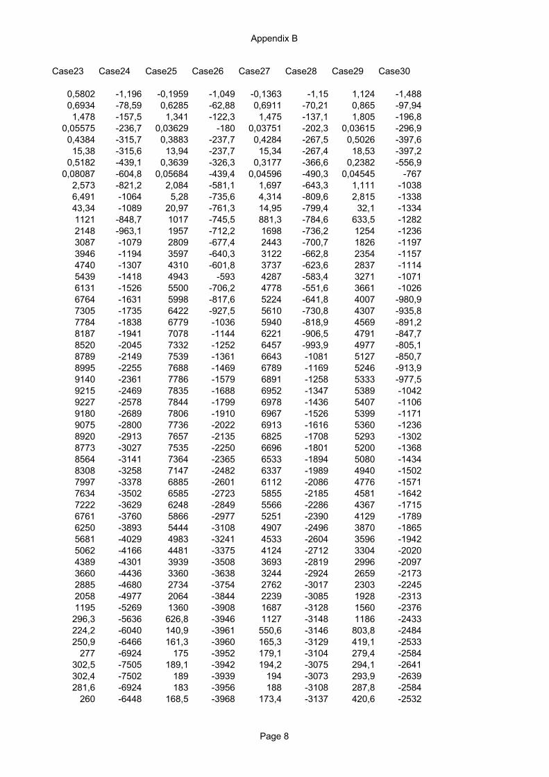
Appendix B
Case23 Case24 Case25 Case26 Case27 Case28 Case29 Case30
0,5802 -1,196 -0,1959 -1,049 -0,1363 -1,15 1,124 -1,4880,6934 -78,59 0,6285 -62,88 0,6911 -70,21 0,865 -97,94
1,478 -157,5 1,341 -122,3 1,475 -137,1 1,805 -196,80,05575 -236,7 0,03629 -180 0,03751 -202,3 0,03615 -296,9
0,4384 -315,7 0,3883 -237,7 0,4284 -267,5 0,5026 -397,615,38 -315,6 13,94 -237,7 15,34 -267,4 18,53 -397,2
0,5182 -439,1 0,3639 -326,3 0,3177 -366,6 0,2382 -556,90,08087 -604,8 0,05684 -439,4 0,04596 -490,3 0,04545 -767
2,573 -821,2 2,084 -581,1 1,697 -643,3 1,111 -10386,491 -1064 5,28 -735,6 4,314 -809,6 2,815 -133843,34 -1089 20,97 -761,3 14,95 -799,4 32,1 -13341121 -848,7 1017 -745,5 881,3 -784,6 633,5 -12822148 -963,1 1957 -712,2 1698 -736,2 1254 -12363087 -1079 2809 -677,4 2443 -700,7 1826 -11973946 -1194 3597 -640,3 3122 -662,8 2354 -11574740 -1307 4310 -601,8 3737 -623,6 2837 -11145439 -1418 4943 -593 4287 -583,4 3271 -10716131 -1526 5500 -706,2 4778 -551,6 3661 -10266764 -1631 5998 -817,6 5224 -641,8 4007 -980,97305 -1735 6422 -927,5 5610 -730,8 4307 -935,87784 -1838 6779 -1036 5940 -818,9 4569 -891,28187 -1941 7078 -1144 6221 -906,5 4791 -847,78520 -2045 7332 -1252 6457 -993,9 4977 -805,18789 -2149 7539 -1361 6643 -1081 5127 -850,78995 -2255 7688 -1469 6789 -1169 5246 -913,99140 -2361 7786 -1579 6891 -1258 5333 -977,59215 -2469 7835 -1688 6952 -1347 5389 -10429227 -2578 7844 -1799 6978 -1436 5407 -11069180 -2689 7806 -1910 6967 -1526 5399 -11719075 -2800 7736 -2022 6913 -1616 5360 -12368920 -2913 7657 -2135 6825 -1708 5293 -13028773 -3027 7535 -2250 6696 -1801 5200 -13688564 -3141 7364 -2365 6533 -1894 5080 -14348308 -3258 7147 -2482 6337 -1989 4940 -15027997 -3378 6885 -2601 6112 -2086 4776 -15717634 -3502 6585 -2723 5855 -2185 4581 -16427222 -3629 6248 -2849 5566 -2286 4367 -17156761 -3760 5866 -2977 5251 -2390 4129 -17896250 -3893 5444 -3108 4907 -2496 3870 -18655681 -4029 4983 -3241 4533 -2604 3596 -19425062 -4166 4481 -3375 4124 -2712 3304 -20204389 -4301 3939 -3508 3693 -2819 2996 -20973660 -4436 3360 -3638 3244 -2924 2659 -21732885 -4680 2734 -3754 2762 -3017 2303 -22452058 -4977 2064 -3844 2239 -3085 1928 -23131195 -5269 1360 -3908 1687 -3128 1560 -2376
296,3 -5636 626,8 -3946 1127 -3148 1186 -2433224,2 -6040 140,9 -3961 550,6 -3146 803,8 -2484250,9 -6466 161,3 -3960 165,3 -3129 419,1 -2533
277 -6924 175 -3952 179,1 -3104 279,4 -2584302,5 -7505 189,1 -3942 194,2 -3075 294,1 -2641302,4 -7502 189 -3939 194 -3073 293,9 -2639281,6 -6924 183 -3956 188 -3108 287,8 -2584
260 -6448 168,5 -3968 173,4 -3137 420,6 -2532
Page 8

Appendix B
237,8 -6037 146,9 -3974 551,2 -3158 805,9 -2483319,8 -5670 625,9 -3962 1126 -3163 1188 -24321218 -5306 1357 -3927 1684 -3147 1562 -23762072 -4996 2058 -3864 2235 -3105 1930 -23132886 -4710 2726 -3774 2752 -3037 2305 -22453657 -4463 3341 -3656 3227 -2943 2660 -21724383 -4324 3921 -3529 3675 -2840 2998 -20975058 -4184 4460 -3398 4100 -2735 3304 -20205676 -4043 4957 -3267 4508 -2629 3598 -19426247 -3903 5417 -3136 4880 -2524 3873 -18656762 -3765 5835 -3008 5221 -2421 4129 -17897230 -3630 6213 -2882 5537 -2319 4370 -17147648 -3499 6553 -2759 5821 -2220 4583 -16418012 -3371 6850 -2639 6076 -2124 4775 -15718325 -3248 7107 -2523 6302 -2030 4941 -15028580 -3127 7322 -2408 6495 -1937 5082 -14348778 -3008 7489 -2295 6655 -1846 5197 -13678921 -2890 7612 -2184 6779 -1756 5292 -13019049 -2774 7690 -2072 6866 -1667 5356 -12369137 -2658 7753 -1962 6913 -1578 5403 -11709162 -2543 7791 -1852 6925 -1489 5407 -11069123 -2429 7778 -1743 6898 -1401 5384 -10419027 -2316 7732 -1635 6833 -1314 5337 -977,28868 -2204 7629 -1527 6731 -1227 5246 -913,68655 -2094 7476 -1420 6582 -1141 5126 -850,38381 -1984 7271 -1314 6392 -1055 4978 -788,28074 -1875 7012 -1207 6155 -969,4 4791 -824,77694 -1767 6710 -1101 5872 -883,8 4566 -867,27234 -1659 6353 -994,4 5537 -797,7 4305 -910,56691 -1549 5922 -886,6 5149 -710,9 4004 -954,56082 -1438 5426 -777,4 4703 -622,8 3659 -998,45399 -1325 4865 -666,4 4210 -625,6 3270 -10424687 -1209 4230 -648,2 3657 -666,9 2835 -10843916 -1091 3517 -688,1 3042 -707,5 2352 -11253048 -970,5 2727 -727,1 2360 -747,2 1822 -11652101 -849,4 1878 -765,2 1619 -785,8 1251 -12031070 -798,9 948,6 -806,3 813,5 -841,6 631 -1246
40,42 -1089 18,62 -875,1 11,93 -908,7 32,4 -12945,968 -1057 4,691 -845,6 3,72 -915,4 2,836 -12862,256 -804,5 1,781 -669,7 1,403 -728 1,084 -997,4
0,2615 -582,2 0,2258 -505,8 0,1942 -553 0,1492 -730,10,4467 -411,7 0,2765 -369 0,2305 -405,6 0,1977 -518,9
16,81 -284,1 15,27 -257,8 16,88 -283,9 20,72 -360,30,2997 -284,6 0,2618 -258,4 0,2883 -284,5 0,3395 -360,9
0,03789 -203,5 0,01837 -184,8 0,01647 -203,5 0,01633 -260,90,3789 -121,6 0,3432 -110,3 0,3782 -121,5 0,4605 -160,60,2085 -50,66 0,1667 -45,96 0,1839 -50,59 0,2491 -70,85
8,334 -0,1158 7,556 -0,09375 8,316 -0,1017 10,19 -0,1179
Page 9

Project: 100-411-1
Designer: JNt
Systemberäkning, styv grundläggning
Last calc. started at: 2021-02-02 07:30:00
Calculated with version: 4.3.23
Last save at: 2021-02-02 07:29:55
Model ID: 58327530
Project File Name: 100-411-1BRIGADE/Standard version 4.3.23
Date: 2021-02-02
Time: 09:34:08
Page: 1 of 2
Result Set Name: Trafiklaster
Case 1: Classification vehicle a (no surface load), Max
Bending Moment Mh (kNm)
Case 2: Classification vehicle a (no surface load), Min
Bending Moment Mh (kNm)
Case 3: Classification vehicle b (no surface load), Max
Bending Moment Mh (kNm)
Case 4: Classification vehicle b (no surface load), Min
Bending Moment Mh (kNm)
Case 5: Classification vehicle c (no surface load), Max
Bending Moment Mh (kNm)
Case 6: Classification vehicle c (no surface load), Min
Bending Moment Mh (kNm)
Case 7: Classification vehicle d (no surface load), Max
Bending Moment Mh (kNm)
Case 8: Classification vehicle d (no surface load), Min
Bending Moment Mh (kNm)
Case 9: Classification vehicle e (no surface load), Max
Bending Moment Mh (kNm)
Case 10: Classification vehicle e (no surface load), Min
Bending Moment Mh (kNm)
Case 11: Classification vehicle f (no surface load), Max
Bending Moment Mh (kNm)
Case 12: Classification vehicle f (no surface load), Min
Bending Moment Mh (kNm)
Case 13: Classification vehicle g (no surface load), Max
Bending Moment Mh (kNm)
Case 14: Classification vehicle g (no surface load), Min
Bending Moment Mh (kNm)
Case 15: Classification vehicle h (no surface load), Max
Bending Moment Mh (kNm)
Case 16: Classification vehicle h (no surface load), Min
Bending Moment Mh (kNm)
-1.00e+04
-8.75e+03
-7.50e+03
-6.25e+03
-5.00e+03
-3.75e+03
-2.50e+03
-1.25e+03
0.00e+00
1.25e+03
2.50e+03
3.75e+03
5.00e+03
6.25e+03
7.50e+03
8.75e+03
1.00e+04
1
2
3
4
5
6
7
8
9
10
11
12
13
14
15
16
17
18
19
20
21
22
23
24
25
26
27
28
29
30

CHALMERS Architecture and Civil Engineering, Master’s Thesis ACEX30 64
DEPARTMENT OF ARCHITECTURE AND CIVIL ENGINEERING DIVISION OF STRUCTURAL ENGINEERING
CONCRETE STRUCTURES
CHALMERS UNIVERSITY OF TECHNOLOGY
Gothenburg, Sweden 2021
www.chalmers.se
daniaspe
Markera
CHALMERS Architecture and Civil Engineering, Master’s Thesis ACEX30 64
daniaspe
Markera
rchitecture and Civil Engineering, Master’s Thesis ACEX30 6
daniaspe
Markera
CHALMERS Architecture and Civil Engineering, Master’s Thesis ACEX30 64
daniaspe
Rektangel