International Journal of Computer Assisted Radiology and Surgeryhttps://doi.org/10.1007/s11548-019-01914-4

ORIG INAL ART ICLE

Early esophageal adenocarcinoma detection using deep learningmethods

Noha Ghatwary1,2 ·Massoud Zolgharni1 · Xujiong Ye1

Received: 11 January 2018 / Accepted: 7 January 2019© The Author(s) 2019

AbstractPurpose This study aims to adapt and evaluate the performance of different state-of-the-art deep learning object detectionmethods to automatically identify esophageal adenocarcinoma (EAC) regions from high-definition white light endoscopy(HD-WLE) images.Method Several state-of-the-art object detection methods using Convolutional Neural Networks (CNNs) were adapted toautomatically detect abnormal regions in the esophagus HD-WLE images, utilizing VGG’16 as the backbone architecture forfeature extraction. Those methods are Regional-based Convolutional Neural Network (R-CNN), Fast R-CNN, Faster R-CNNand Single-Shot Multibox Detector (SSD). For the evaluation of the different methods, 100 images from 39 patients that havebeen manually annotated by five experienced clinicians as ground truth have been tested.Results Experimental results illustrate that the SSD and Faster R-CNN networks show promising results, and the SSDoutperforms other methods achieving a sensitivity of 0.96, specificity of 0.92 and F-measure of 0.94. Additionally, theAverage Recall Rate of the Faster R-CNN in locating the EAC region accurately is 0.83.Conclusion In this paper, recent deep learning object detection methods are adapted to detect esophageal abnormalitiesautomatically. The evaluation of the methods proved its ability to locate abnormal regions in the esophagus from endoscopicimages. The automatic detection is a crucial step that may help early detection and treatment of EAC and also can improveautomatic tumor segmentation to monitor its growth and treatment outcome.

Keywords Deep learning · Esophageal adenocarcinoma detection · Barrett’s esophagus · HD-WLE

Introduction

Amajor health problem that has been emerging is esophagealadenocarcinoma (EAC) which is considered the early stageof esophageal cancer. Studies show that esophageal cancerpatients hold a 5-year survival rate of only 18.8% [1]. The pri-mary premalignant cause of reaching esophagealmalignancyis Barrett’s esophagus (BE) [2,3], where the development ofhealthy cells in the esophagus lining into columnar mucosa

B Noha Ghatwarynghatwary@lincoln.ac.uk; noha.ghatwary@aast.edu

Massoud Zolgharnimzolgharni@lincoln.ac.uk

Xujiong Yexye@lincoln.ac.uk

1 University of Lincoln, Lincoln, UK

2 Arab Academy for Science and Technology, Alexandria,Egypt

through metaplastic change leads to EAC [4]. The earlydetection and treatment of EAC may help in increasing thesurvival chance of the patient [5].

The process of detection is done through endoscopicexamination, high-definition white light endoscopy (HD-WLE) is the primary tool used [6], and the cell deformationstages are confirmed by taking biopsy samples from thesurface of the esophagus lining [7]. The appearance andproperties of the BE or EAC have challenges in the detec-tion process as it can be located randomly throughout theesophagus tube [8]. Also, the accurate detection requiresa physician with significant experience and they are oftenoverlooked during endoscopy surveillance [9]. In addition tothat, patients are required to have regular follow-ups throughendoscopy examination to control the development of abnor-malities into later stages. With the increase in the numberof patients, computer-aided detection (CAD) systems havegrabbed attention more frequently. There exists an amountof research available in the literature for automatic detec-

123

International Journal of Computer Assisted Radiology and Surgery

tion, segmentation and classification that employs severalendoscopies such as white light endoscopy (WLE), nar-row band imaging (NBI), volumetric laser endomicroscopy(VLE), confocal laser endomicroscopy (CLE) and chro-moendoscopy; these methods are summarized and discussedin [10,11]. In the next section, an overview of the pre-vious studies on EAC detection from HD-WLE will bediscussed.

Recently, deep learning (DL) has been tremendouslyuseful in a wide range of different applications, such as com-puter vision, natural language processing, medical imaginganalysis and much more [12]. Deep learning, specifically,Convolutional Neural Networks (CNNs), has become a con-ventional technique in medical image analysis (detection,classification, segmentation, etc.) [13]. In this work, we takeadvantage of recent development in object detectionmethodsthat utilize CNNs to locate EAC abnormalities in esophagusendoscopic images by employing the state-of-the-art CNNmethods and evaluating them on our dataset. To the best ofour knowledge, no work has been addressed before to com-prehensively assess the performance of different CNN-baseddetection methods for detecting tumors in esophageal endo-scopic images.

The rest of the paper is organized as follows: the sec-ond section represents the related work of EAC detectionfrom HD-WLE images. In the third section the materials andmethods are discussed, where a brief description of state-of-the-art deep learning object detection methods is presented,and the dataset used is described, while the experimentalresults are demonstrated in the fourth section. Finally, theevaluated results are discussed in the fifth section and con-cluded in the sixth section.

Related work

Different studies have been conducted in the literature thatfocused on the detection of BE and EAC using severalendoscopic tools. These methods are discussed in [10,11].In this section, we will only discuss previous methodsthat address the detection of EAC abnormalities using thesame HD-WLE images dataset that we used in our evalua-tion.

An evaluation of different texture features extracted fromHD-WLE Barrett’s esophagus images was proposed by Ses-tio et al. [14] and Sommen [15]. This study extracted thefollowing features: texture spectrum, histogram of orientedgradients (HOG), local binary pattern (LBP), Gray LevelCo-occurrence Matrix (GLCM), fourier feature, dominantneighbor structure (DNS) and gabor features to comparebetween them on the effect of EAC detection. As a pre-processing phase, the irrelevant textures tiles have beendiscarded before applying the classifier. Additionally, the

principal component analysis (PCA) was used for reduc-ing the features dimension, and they were classified usingthe support vector machine (SVM). After testing differentcombinations, this comparison concluded that the mergebetween gabor and color features achieved the best resultscompared to other combination of extracted features achiev-ing an overall accuracy of 96.48%. Based on the con-clusion in [14,15], Sommen et al. [9] proposed a CADsystem to detect and annotate EAC regions in HD-WLE.Using a Leave-One-Patient-Out Cross-Validation (LOPO-CV) approach the experiments had an 85.7% accuracycompared to the annotation of the specialist with a recallof 0.95 and precision of 0.75 using the SVM classifier onthe extracted gabor and color features. More tests wereconducted in [16] with the same model on a more sub-stantial dataset that resulted in a sensitivity of 0.86 and aspecificity of 0.87 when using SVM and 0.90 and 0.75 forthe precision when classified using the Random forest in[17].

Souza Jr. et al. [18] proposed an investigation of the fea-sibility of the SVM to classify lesions in Barrett’s esophagusbased on Speed-Up Robust Features (SURF) descriptors.Two experiments were carried out by extracting the SURFfeatures from the full image and another from the EACground truth regions annotated by experts. The results basedon full images analysis showed a sensitivity of 0.77 and speci-ficity of 0.82, while the abnormal region-based approachhas a sensitivity of 0.89 and specificity of 0.95. Theseresults were analyzed based on the LOPO-CV approach andSVM classifier. Later on, Souza Jr. et al. [19] proposed anOptimum-Path Forest (OPF) classifier to identify BE andadenocarcinoma HD-WLE images. Features were extractedfrom the images using the Scale-Invariant Feature Transform(SIFT) and the SURF to design a bag of visual words (BoW)to be an input for the OPF and SVM classifiers. Resultsshowed that the OPF outperformed the SVM with sensitiv-ity of 73.2% (SURF)–73.5% (SIFT), specificity of 78.2%(SURF)–80.6% (SIFT) and accuracy of 73.8% (SURF)–73.2% (SIFT).

Mendel et al. [20] studied the analysis of BE using CNNto classify patches in an HD-WLE image into cancerous andnon-cancerous. Regarding the experiments, the image wasfirst divided into non-overlapping 224 × 224 patches andsampled as cancerous and non-cancerous based on a certainthreshold t. Each patch has an output probability that wascompared to the value t to decide whether it is a cancer-ous region or not. The deep residual network (ResNet) [21]was used as the deep learning method for feature extractionand classification from each patch. After testing the perfor-mance of classification at seven different values for thresholdt, the best performance was achieved at t = 0.8 resulting ina sensitivity of 0.94, specificity of 0.88 and F-measure of0.91.

123

International Journal of Computer Assisted Radiology and Surgery

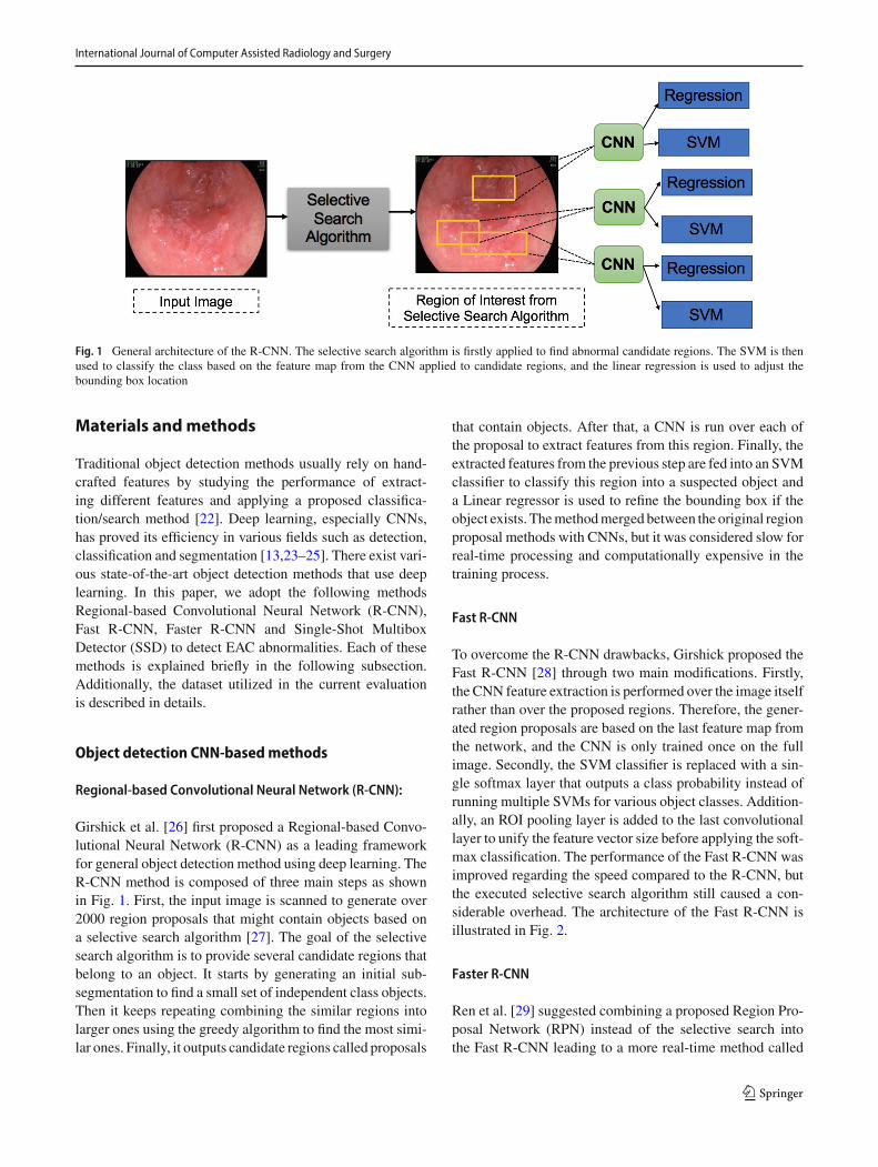
Fig. 1 General architecture of the R-CNN. The selective search algorithm is firstly applied to find abnormal candidate regions. The SVM is thenused to classify the class based on the feature map from the CNN applied to candidate regions, and the linear regression is used to adjust thebounding box location

Materials andmethods

Traditional object detection methods usually rely on hand-crafted features by studying the performance of extract-ing different features and applying a proposed classifica-tion/search method [22]. Deep learning, especially CNNs,has proved its efficiency in various fields such as detection,classification and segmentation [13,23–25]. There exist vari-ous state-of-the-art object detection methods that use deeplearning. In this paper, we adopt the following methodsRegional-based Convolutional Neural Network (R-CNN),Fast R-CNN, Faster R-CNN and Single-Shot MultiboxDetector (SSD) to detect EAC abnormalities. Each of thesemethods is explained briefly in the following subsection.Additionally, the dataset utilized in the current evaluationis described in details.

Object detection CNN-basedmethods

Regional-based Convolutional Neural Network (R-CNN):

Girshick et al. [26] first proposed a Regional-based Convo-lutional Neural Network (R-CNN) as a leading frameworkfor general object detection method using deep learning. TheR-CNN method is composed of three main steps as shownin Fig. 1. First, the input image is scanned to generate over2000 region proposals that might contain objects based ona selective search algorithm [27]. The goal of the selectivesearch algorithm is to provide several candidate regions thatbelong to an object. It starts by generating an initial sub-segmentation to find a small set of independent class objects.Then it keeps repeating combining the similar regions intolarger ones using the greedy algorithm to find the most simi-lar ones. Finally, it outputs candidate regions called proposals

that contain objects. After that, a CNN is run over each ofthe proposal to extract features from this region. Finally, theextracted features from the previous step are fed into an SVMclassifier to classify this region into a suspected object anda Linear regressor is used to refine the bounding box if theobject exists. Themethodmerged between the original regionproposal methods with CNNs, but it was considered slow forreal-time processing and computationally expensive in thetraining process.

Fast R-CNN

To overcome the R-CNN drawbacks, Girshick proposed theFast R-CNN [28] through two main modifications. Firstly,the CNN feature extraction is performed over the image itselfrather than over the proposed regions. Therefore, the gener-ated region proposals are based on the last feature map fromthe network, and the CNN is only trained once on the fullimage. Secondly, the SVM classifier is replaced with a sin-gle softmax layer that outputs a class probability instead ofrunning multiple SVMs for various object classes. Addition-ally, an ROI pooling layer is added to the last convolutionallayer to unify the feature vector size before applying the soft-max classification. The performance of the Fast R-CNN wasimproved regarding the speed compared to the R-CNN, butthe executed selective search algorithm still caused a con-siderable overhead. The architecture of the Fast R-CNN isillustrated in Fig. 2.

Faster R-CNN

Ren et al. [29] suggested combining a proposed Region Pro-posal Network (RPN) instead of the selective search intothe Fast R-CNN leading to a more real-time method called

123

International Journal of Computer Assisted Radiology and Surgery

Fig. 2 General architecture of the Fast R-CNN. The CNN is applied to the input image to extract the feature map, and the selective search algorithmis performed to find abnormal candidate regions. The ROI is applied after that to unify the feature vector size for classification using Softmaxclassifier

Fig. 3 An example of different anchor boxes with different sizes and ratios for a specific location in the RPN stage

Faster R-CNN. The proposed RPN generates region propos-als for each location using the last feature map producedfrom the CNN based on anchor boxes. The anchor boxes aredetections boxes that have different sizes and ratios that arecompared to the ground truth during the training process. Foreach location in the feature map, there are K different anchorboxes centered around it as shown in Fig. 3. The total numberof anchor boxes per image is (K × W × H) where the Wand H are the sizes of the last feature map. During training,each generated anchor box is compared to the ground truthobject location. Boxes that overlap the ground truth with anIntersection over Union (IoU) based on a certain thresholdare considered as an object (no class specified). The IoU iscalculated as follows:

IoU = Agt ∩ Ap

Agt ∪ Ap(1)

where Agt is the area of the ground truth bounding box whileAp is the predicted bounding box from the regression layer.The selected anchor boxes are passed on as region proposalsfrom RPN stage with a classification score for each box andfour coordinates that represent the location of this object.

Some region proposals highly overlap each other; there-fore, non-maximum suppression (NMS) is used to prune theredundant regions leading to a reduced number of region pro-posals. Later on, the selected region proposals are fed intothe next phase as in Fast R-CNN. The ROI pooling dividesthe input feature map from candidate anchor boxes into afixed number of almost equal regions. Maxpooling is appliedto these regions; consequently, the output from the phase isalways fixed size regardless of the input size. One of themainbenefits of the Faster R-CNN is that the convolutional layerbetween two networks (RPN and Fast R-CNN) is shared asshown in Fig. 4 rather than learning two separate networks.

Single-Shot Multibox Detector (SSD)

Liu et al. [30] presented a Single-Shot Multibox Detector(SSD). SSD is considered a faster deep learning object detec-tion method compared to previously discussed methods asit generates the predicting bounding box and classifies theobject within it in a single operation while processing theimage. During the training process, the SSD takes the imageand the ground truth as inputs. Following that, the image is

123

International Journal of Computer Assisted Radiology and Surgery

Fig. 4 General architecture of the Faster R-CNN. The CNN is applied to the input image to extract the feature map that is later used by both theRPN and the ROI pooling layers (Feature map is shared between both). The RPN outputs the classification score and bounding box location of thecandidate region proposals that are passed on to the next stage. The ROI layer unifies the feature vector size of the candidate region proposal thatis classified using softmax

Fig. 5 General architecture of the SSD [30]. The SSD is a single unified network for both testing and inference

passed through a series of convolutional layers that are com-bined throughout the network as shown in Fig. 5. The SSDgenerates a list of bounding boxes for each location using pri-ors (i.e., same as anchors in Faster R-CNN) and then adjustsit to be close to the ground truth location as much as possi-ble. Although the number of generated boxes from SSD isconsidered a huge number compared to the other methods,it does not guarantee to have an object inside it. An NMSis applied to minimize the number of boxes by grouping thehighly overlapping regions and choosing the box with thehighest confidence.

Additionally, negative samples are kept with a ratio of3:1 compared to positive samples in order to apply hard-negativemining. The hard-negativemining helps the networkto better learn the incorrect detection leading to more accu-rate results. The backbone CNN network used in the FasterR-CNN and the SSD is the VGG’16 [31] after discardingthe fully connected layer and using its feature map. Oneof the main reasons for using the VGG’16 is that it hasa very high performance toward image classification prob-lems.

In this paper, we evaluate the performance of the describeddeep learning object detection methods using the VGG’16 asthe backbone network to identify the EAC abnormalities inthe HD-WLE images automatically.

Dataset

Adataset composed of 100HD-WLE images of lower esoph-agus provided by the Endoscopic Vision Challenge MICCAI2015 [32] and [9] is used in the evaluation. The 100 imageswere divided into 50 images with non-cancerous regions(Fig. 6a) and another 50 with EAC (Fig. 6b). The imageswere gathered from 39 patients, among those patients, 22patients diagnosed with esophageal adenocarcinoma and 17patients with non-cancerous Barrett’s. Different numbers ofimages were captured from each patient resulting in a variednumber from one to eight images per patient. Lesions foundin the abnormal images have been annotated by five lead-ing experts in the field to obtain golden standards as shownin Fig. 6c. Due to the differences in manual segmentationfrom one expert to another, we used the largest intersection

123

International Journal of Computer Assisted Radiology and Surgery

(a) Non-Cancer Patient (b) Cancerous Patient (c) Annotation by experts

Fig. 6 Examples of the HD-WLE images from the provided dataset showing a non-cancerous Barrett’s patient, b EAC patient and c annotationfrom five different experts

area between the annotations from all the experts during thetraining and testing phase.

Experiments

In this section, we first give details about the implementationsetup for the CNN methods. Then, the measures used in theevaluation process are described. Finally, we evaluate theperformance of the detection methods on our dataset.

Experimental setup

Due to the limited publicly available dataset, we performedan addition data augmentation to the training data by flippingalong the axial plane and rotation in different angleswith 90◦,180◦ and 270◦.

For implementation, we adopt the Keras library [33]based on Python to train and test the different deep learn-ing object detection models on a single Nvidia 1080Ti GPU.The VGG’16 was employed as the backbone CNN networkfor the four discussed models, which has been trained fromscratch on the dataset after augmentation. Each model wastrained for 5000 iterationswith the learning rate set to 0.0001.Additionally, the images were used with its original size(1600 × 1200) for the following networks R-CNN, Fast R-CNN and Faster R-CNN, while in the SSD, the images wererescaled to 300 × 300.

During the training process, the anchor boxes sizes andratios for the RPN stage in the Faster R-CNN were set tothe default setting as proposed in [29], where there exist K= 9 anchors at each location with three scales (1282, 2562

and 5122 pixels) and three aspect ratios (1:1, 1:2 and 2:1).Furthermore, the anchor boxes are comparedwith the groundtruth to generate the RPN proposals, and the region with anIoU (Eq. 1) greater than 0.7 is considered as a proposal. Onthe other hand, the SSD uses multiple feature maps to predictthe target location and calculate a confidence score. In theevaluation, the features are extracted at convolutional layers

4 and 7. Also, the NMS was set to 0.7 for bounding boxselection.

Evaluationmeasures

To assess the performance of the CNNobject detectionmeth-ods in detecting the tumor regions, we employ the AverageRecall Rate (ARR) and Average Precision Rate (APR) [34],tomeasure the accuracy of the detected bounding box in com-parison to the ground truth region in the cancerous images.Also, sensitivity (SE), specificity (SP) and the F-measure(FM) are measured over all the test images (non-cancerousand cancerous) as follows:

ARR = 1

N

N∑

I=1

BgI ∩ Bp

I

BrmgI

(2)

APR = 1

N

N∑

I=1

BgI ∩ Bp

I

BpI

(3)

SE = TP

TP + FN(4)

SP = TN

TN + FP(5)

FM = 2 · TP2 · TP + FP + FN

(6)

where N is the total number of images, the Bg is the groundtruth bounding box area of the tumor region while Bp is thearea of predicted bounding box proposed by the detectionmethod. Taking into consideration the (x, y) coordinates asthe location of the upper left corner of both boxes to computethe intersection, all measures have been assessed in referenceto the cancerous patients, True Positive (TP) the number ofcancerous images that had correct prediction, True Negative(TN) the number of non-cancerous images that had correctprediction, False Negative (FN) number of cancerous imagesthat had no prediction and False Positive (FP) number of non-cancerous images that had regions predicted as cancerous.

123

International Journal of Computer Assisted Radiology and Surgery

Results

The four deep learning object detection approaches discussedin “Object detection CNN based methods” section have beencarried on the available dataset after augmentation. The fivemeasures defined in Eqs. 2–6 were used to evaluate detectionperformances. First, the ARR and APR were used to evalu-ate the bounding box accuracy. A higher APR demonstratesthat a more significant region is overlapping between the pre-dicted region and the ground truth, and a higher ARR showsthat the tumor region generated by the detection methodexcludes more non-cancerous areas. Moreover, the sensitiv-ity, specificity and F-measure rates were measured, wherethe number of the missed region in a cancerous patient (nodetection) and any false prediction in normal patient imagesaffected the results. Additionally, if the IoU value betweenthe generated bounding box and the ground truth is less than0.5, then the produced bounding box is considered to be afalse prediction (non-cancerous). Furthermore, the time forthe detection processes for each method was measured inseconds during the testing phase.

The experiments have been carried out using three typesof validation. Experiment 1: from the 39 patients, 60%were used for training [21 patients (12 cancerous, 9 non-cancerous Barrett’s)], 20% for validation [9 patients (5cancerous, 4 non-cancerous Barrett’s)] and 20% for test-ing [9 patients (5 cancerous, 4 non-cancerous Barrett’s)].The experiments were carried twice to verify the resultsusing more cases by changing the patients dataset betweenthe validation and testing sets in the second experiment.Therefore, the results presented in Table 1 are based on atotal of 18 patients (10 cancerous and 8 non-cancerous Bar-rett’s) that are entirely different from the dataset used fortraining the model. Experiment 2: The dataset was eval-uated based on 5-fold-cross-validation (5-fold-CV), wherethe dataset is divided into 5-fold randomly. (Each fold willhold 7–8 patients.) The results of the second experimentare shown in Table 2. Experiment 3: Leave-One-Patient-Outcross-validation (LOPO-CV) is applied to compare the fourdetection methods. Table 3 demonstrates the results fromLOPO-CV experiment in addition to a comparison with twoof state-of-the-art (Mendel et al. [20] and Sommen et al.[16]) methods that use the same dataset. The results of thethree experiments will be discussed further in the followingsection.

Furthermore, the bounding box results from each methodhave been provided on some sample images shown in Fig. 7and compared to the ground truth bounding box. The figureshows different samples of the true and false positives detec-tion. An example from one non-cancerous image that hadfalse prediction by the R-CNN and Fast R-CNN method isshown in Fig. 7c, and another one by the R-CNN is shown inFig. 7l. Moreover, Fig. 7j illustrates the detection of Faster

Table 1 Average Recall Rate (ARR), Average Precision Rate (APR),sensitivity (SE) and specificity (SP) and F-measure (FM) for the state-of-the-art object detection deep learning methods on the EAC datasetbased on 60% training and 40% testing

Method APR ARR SE SP FM Time (s)

R-CNN 0.43 0.41 0.47 0.41 0.44 13.38–37.81

Fast R-CNN 0.66 0.37 0.53 0.57 0.55 0.65–2.1

Faster R-CNN 0.50 0.78 0.72 0.83 0.83 0.3–0.45

SSD 0.69 0.81 0.93 0.93 0.93 0.1–0.2

Bold values represent the highest values

Table 2 Average Recall Rate (ARR), Average Precision Rate (APR),sensitivity (SE) and specificity (SP) and F-measure (FM) for the state-of-the-art object detection deep learning methods on the EAC datasetbased on 5-fold-CV

Method APR ARR SE SP FM

R-CNN 0.48 0.41 0.50 0.40 0.48

Fast R-CNN 0.62 0.43 0.64 0.64 0.64

Faster R-CNN 0.68 0.83 0.78 0.80 0.79

SSD 0.70 0.79 0.90 0.88 0.88

Bold values represent the highest values

Table 3 Average Recall Rate (ARR), Average Precision Rate (APR),sensitivity (SE), specificity (SP) and F-measure (FM) for the state-of-the-art object detection deep learningmethods on the EACdataset basedon LOPO-CV

Method SE SP FM

R-CNN 0.60 0.56 0.59

Fast R-CNN 0.64 0.60 0.63

Faster R-CNN 0.88 0.86 0.87

SSD 0.96 0.92 0.94

Mendel et al. [20] 0.94 0.88 0.91

Sommen et al. [16] 0.86 0.87 0.87

Bold values represent the highest values

R-CNN and SSD only as the other two methods failed tofind an EAC region. The rest of the figures demonstrate theperformance of the four models in detecting the abnormalregions in minor and complex tumors.

Discussion

CAD has been acting as an essential tool in clinical practiceand research by providing a second opinion to the clinician.With the evolving of the use of deep learning methods inimplementing CADmethods in various fields, there has beena tremendous improvement in accuracy. Multiple CAD sys-tems have been proposed in the literature that mainly reliedon handcrafted features to detect EAC abnormalities in endo-scopic images. Only one method used the deep learning to

123

International Journal of Computer Assisted Radiology and Surgery

(a) Cancerous groundtruth (b) Cancerous groundtruth (c) Normal groundtruth

(d) Cancerous Prediction (e) Cancerous Prediction (f)False prediction

(g) Cancerous groundtruth (h) Cancerous groundtruth (i) Normal groundtruth

(j) Cancerous Prediction (k) Cancerous Prediction (l) False prediction

Fig. 7 Bounding box ground truth based on experts annotation and the output from the R-CNN, Fast R-CNN, Faster R-CNN and SSD when using5-fold-CV from different patients showing correct prediction in d, e, j and k with different scores and a false prediction on a non-cancerous patientin f and l

classify the patches inside image into cancerous and non-cancerous [20].

The APR and ARR are used to measure the performanceof the detection methods by evaluating the output bound-ing box in cancerous images only. They both measure theoverlapping region between the predicted bounding box andground truth. As shown in Table 1, the APR results for theFast R-CNN and the SSD achieved 0.66 and 0.69, respec-tively. Additionally, the APR results from Table 2 show thatthe Faster R-CNN achieved 0.68, while the SSD achieved

0.70. From both tables, the SSD proved the ability to detect agreater abnormal region that overlappedwith the ground truthgenerated by experts compared to the other three CNNmeth-ods. Moreover, the ARR from these two tables, the FasterR-CNN and SSD outperform the Fast R-CNN and R-CNNwith results of 0.78 and 0.81 from Table 1 and 0.83 and 0.79from Table 2. The results indicate that the SSD and FasterR-CNNwere able to detect fewer false positive regions (non-cancerous areas) inside the generated bounding box for theabnormal area.

123

International Journal of Computer Assisted Radiology and Surgery

Additionally, the sensitivity, specificity and F-measureare measured for the three experimental validation methods.Results in Table 1 are based only on 18 patients (10 cancer-ous and 8 non-cancerous Barrett’s) as described previouslyin “Results” section. The SSD outperforms among the com-pared methods with a result of 0.93 for the three measures.The high sensitivity of the SSD result from this table indi-cates that it had a good performance in detectingEAC regionsfrom the cancerous images and less false bounding boxes inthe non-cancerous Barrett’s images. The Faster R-CNN fol-lowed by with results of 0.72 for the sensitivity and 0.83 forboth the specificity and F-measure.

From Table 2 based on 5-fold-CV. The SSD surpasses theother three methods with a sensitivity of 0.90, both speci-ficity and F-measure of 0.88. The results demonstrate thatthe SSD had a high performance in generating boundingboxes that located in abnormal regions throughout the testingdataset and less false ones. For the Faster R-CNN as shownin Table 2, the results of the sensitivity were 0.78 and 0.80for the specificity and 0.79 for the F-measure demonstratingan acceptable performance.

As a further study, a comparison of the results with otherstate-of-the-art models provided by Mendel et al. [20] andSommen et al. [16] is illustrated in Table 3. For a fair eval-uation, we employ the same validation method LOPO-CV.Firstly, the sensitivity was evaluated, and the SSD achievedthe highest performance among the four deep learning meth-ods and surpassed the results of [20] by 2% and [16] by 10%.Also, the Faster R-CNN outperformed against [16] by 2%.Additionally, the specificity of the SSD achieved 92% indi-cating the improvement of less false positives regions, whilethe Faster R-CNN achieved 0.86 that is considered compa-rable with results of [20] and [16].

As observed in Tables 2 and 3, the R-CNN and the Fast R-CNN have the lowest performance. The reason behind thisis that both methods rely on selective search algorithm togenerate a region of interest. As explained in the earlier sec-tion, selective search algorithm uses the greedy algorithmto search for a location for object localization. The greedyalgorithm has limitations in finding the optimal solution.Additionally, the grouping process is done based on the colorspace difference and similarity metrics, while for our dataset,it is difficult to differentiate between non-cancerous Barrett’sregions and EAC solely based on color as they both have adarker color than normal regions which might lead to morefalse positives.On the other hand, the use of anchor boxes andpriors in the Faster R-CNN and the SSD helps improve theperformance of generating more candidate regions of inter-est. Furthermore, the results of Table 3, in general, are moreimproved than that in Table 2 as the LOPO-CV allows moredataset to be trained than the 5-fold-CV.

The differences in sensitivity and specificity between thefour object detection methods were statistically evaluated

Table 4 The p-value calculate using the paired t-test to measure thedifference of sensitivity and specificity results between the four deeplearning methods

Method Sensitivity Specificity

R-CNN Fast R-CNN R-CNN Fast R-CNN

Faster R-CNN 0.0049 0.1279 0.0001 0.0443

SSD 0.0012 0.0882 0.0001 0.0036

using the paired t-test at a confidence level of 95%. Theresults of the two-tailed p value of the two best performers(SSD and Faster R-CNN), when compared with the othertwo methods, are illustrated in Table 4. As shown, the dif-ference between the sensitivity and specificity of the SSDand Faster R-CNN was found to be significantly differentwhen they were compared to the R-CNN and Fast R-CNNusing the t-test. Additionally, the t-test was also employed todetermine whether there are any statistical differences in thesensitivity and specificity, obtained using the two validationmethods (i.e., 5-fold-CV and LOPO-CV). The p value of thesensitivity and specificity for each deep learning object detec-tion method was as follows R-CNN (0.0235,0.0068), FastR-CNN (0.3222, 0.1594), Faster R-CNN (0.0238 ,0.0832)and SSD (0.0832, 0.1594). Our analysis based on these pvalues suggests that the two validations for the R-CNN andFaster R-CNN show a significant difference. On the otherhand, the difference in results for the SSD and the fast R-CNN is not statistically significant.

Moreover, the detection time during testing was measuredin seconds for each method as shown in Table 1. The timestarted with a range of 13.38–37.81 s when using the R-CNNand then decreased while using a more updated method. TheR-CNN requires a significant amount of time as it generatesaround 2000 region proposal for each location and then usedto extract features from them using CNN. This leads to arepetition of almost 2000 times to extract features from oneimage. The detection time drops to 0.65–2.1 s when usingthe Fast R-CNN, as the selective search is applied to theextracted features after applying the CNN to the input image.The Faster R-CNN was faster after sharing the weights andfeature map between the RPN and ROI pooling layer result-ing in a range of 0.3–0.5 s to generate detection boundingboxes. The SSD surpassed against the other methods in pre-dicting region in most of the cancerous images with only0.1–0.2 s. The reason for this is that the SSD can localizethe object and classify it in a single forward pass network.We believe that with a more powerful hardware (i.e., NvidiaTitan, Nvidia Tesla V100), the detection speed would be fur-ther increased.

In addition to providing the quantitative evaluation, wealso randomly choose some qualitative results of the deeplearning object detection methods for different cases as

123

International Journal of Computer Assisted Radiology and Surgery

Table 5 Average error presented by each model in capturing non-cancerous regions inside the produced bounding boxes in the EACimages

R-CNN Fast R-CNN Faster R-CNN SSD

Average error 0.388 0.328 0.211 0.197

shown in Fig. 7. For example, Fig. 7e demonstrates that thedifferentmethods can detect somedifficult instances inwhichthe abnormality is located in a small region and is visuallysimilar to other areas inside the same image. Also, in Fig. 7d,k the abnormal areas are present in most of the images. TheSSD and Faster R-CNN show the ability to detect most ofthe EAC area compared to the ground truth. Furthermore,Fig. 7f, l lists some false positive regions detected by theR-CNN and Fast R-CNN. The non-cancerous Barrett’s fromnormal patients have a difference in color in some areas asshown in Fig. 7c, i which makes the detection challenging.The accuracy of this bounding box is discussed earlier usingthe ARR and APR values compared to the ground truth andillustrated in Fig. 7.

The esophagus has a special internal structure that makesit challenging to differentiate between normal and abnor-mal regions. Also, the abnormalities inside the esophagus areparticularly challenging due to its different sizes, locationsand shapes. There exist variations in the size and the loca-tion in the generated bounding boxes from the four models,where eachboxmight includenon-cancerous regions. Table 5calculates the average error presented by each model in cap-turing non-cancerous regions inside the bounding box. Asshown, the R-CNN and Fast R-CNN presented higher errorpercentage compared to the other two models. This indicatesthe bounding box generated by these two methods includeda high ratio of non-cancerous regions. On the other hand,the Faster R-CNN and SSD provided a lower error rate forcontaining non-cancerous areas; therefore, they were able toprovide better bounding boxes localized around the cancer-ous regions.

Conclusion

In this paper, we adapted the state-of-the-art deep learn-ing object detection methods to automatically identify theEAC abnormalities from HD-WLE images. Throughout theevaluation experiments, the SSD has proved to be the lead-ing performance regarding the different evaluationmeasures,with an outstanding result of 0.90 for the sensitivity, 0.88 forthe specificity and 0.88 for the F-measure when evaluatedbased on 5-fold-CV.

Also, the average precision and recall rates are of 0.70and 0.79 for the SSD and 0.68 and 0.83 for the Faster R-

CNN in locating abnormal regions compared to the expert’sannotation. The current study is a step forward to use deeplearning object detection methods to find abnormalities inesophageal endoscopy still image. We mainly focused ondetection by using the bounding boxes to allocate abnormalregions. Additionally, experiments based on LOPO-CV havebeen carried out and compared with other state-of-the-artmethods. The SSD and Faster R-CNN were able to surpassamong the results.

Moreover, figures have been presented to illustrate thegenerated bounding box by each method. There are someerrors introduced by the bounding boxes by the differentmodels that need to be improved. The CNN network usedfor feature extraction can be modified/replaced with adjust-ments in network parameters to improve the final detectionperformance.

Further work will be held to improve the performance ofautomatic EAC detection using the most efficient methodsin current evaluation ( i.e., SSD and Faster R-CNN) and willinclude more patients data to assess the proposed modifiedmethods further.

Compliance with ethical standards

Conflict of interest All the authors declare that they have no conflict ofinterest.

Ethical approval This article does not contain any studies with humanparticipants or animals performed by any of the authors.

Informed consent Informed consent was obtained from all individualparticipants included in the study.

Open Access This article is distributed under the terms of the CreativeCommons Attribution 4.0 International License (http://creativecommons.org/licenses/by/4.0/), which permits unrestricted use, distribution,and reproduction in any medium, provided you give appropriate creditto the original author(s) and the source, provide a link to the CreativeCommons license, and indicate if changes were made.

References

1. https://seer.cancer.gov/statfacts/html/esoph.html2. Rajendra S, Sharma P (2017) Barrett esophagus and intramucosal

esophageal adenocarcinoma. Hematol Oncol Clin 31(3):409–4263. Qi X, Sivak MV, Isenberg G, Willis J, Rollins AM (2006)

Computer-aided diagnosis of dysplasia in Barrett’s esophagususing endoscopic optical coherence tomography. J Biomed Opt11(4):044010

4. Old OJ, Lloyd GR, Nallala J, Isabelle M, Almond LM, Shep-herd NA, Kendall CA, Shore AC, Barr H, Stone N (2017) Rapidinfrared mapping for highly accurate automated histology in Bar-rett’s oesophagus. Analyst 142(8):1227–1234

5. Jiang Y, Gong Y, Rubenstein JH, Wang TD, Seibel EJ (2017)Toward real-time quantification of fluorescence molecular probes

123

International Journal of Computer Assisted Radiology and Surgery

using target/background ratio for guiding biopsy and endoscopictherapy of esophageal neoplasia. J Med Imaging 4(2):024502

6. Behrens A, Pech O, Graupe F, May A, Lorenz D, Ell C (2011) Bar-rett’s adenocarcinoma of the esophagus: better outcomes throughnew methods of diagnosis and treatment. Deutsch rzteblatt Int.108(18):313

7. Trovato C, Sonzogni A, Ravizza D, Fiori G, Tamayo D, DeRoberto G, de Leone A, De Lisi S, Crosta C (2013) Confocal laserendomicroscopy for in vivo diagnosis of Barrett’s oesophagus andassociated neoplasia: a pilot study conducted in a single Italiancentre. Dig Liver Dis 45(5):396–402

8. Ghatwary N, Ahmed A, Ye X, Jalab H (2017) Automatic gradeclassification of Barretts esophagus through feature enhancement.In Medical imaging 2017: computer-aided diagnosis, vol 10134.International Society for Optics and Photonics, p 1013433

9. Van Der Sommen F, Zinger S, Schoon EJ (2014) Supportive auto-matic annotation of early esophageal cancer using local gabor andcolor features. Neurocomputing 144:92–106

10. Ghatwary N, Ahmed A, Ye X (2017) Automated detection of Bar-rett’s esophagus using endoscopic images: a survey. In: Annualconference on medical image understanding and analysis, pp 897–908

11. de Souza LA, Palm C, Mendel R, Hook C, Ebigbo A, Probst A,Messmann H, Weber S, Papa JP (2018) A survey on Barrett’sesophagus analysis using machine learning. Comput Biol Med96:203–213

12. Juefei-Xu F, Boddeti VN, Savvides M, Juefei-Xu F, Boddeti VN,SavvidesM (2017) Local binary convolutional neural networks. In:2017 IEEE conference on computer vision and pattern recognition(CVPR), vol 1

13. Litjens G, Kooi T, Bejnordi BE, Setio AAA, Ciompi F, GhafoorianM, van der Laak JA, vanGinnekenB, SnchezCI (2017)A survey ondeep learning in medical image analysis. Med Image Anal 42:60–88

14. Setio AA, Van Der Sommen F, Zinger S, Schoon EJ, de With PeterHN (2013) Evaluation and comparison of textural feature represen-tation for the detection of early stage cancer in endoscopy. VISAPP1:238–243

15. Van Der Sommen F, Zinger S, Schoon EJ (2013) Computer-aideddetection of early cancer in the esophagus using HD endoscopyimages. In: Medical imaging 2013: computer-aided diagnosis, vol8670. International Society for Optics and Photonics, p 86700V

16. van der Sommen F, Zinger S, Curvers WL, Bisschops R, PechO, Weusten BL, Bergman JJ, Schoon EJ (2016) Computer-aided detection of early neoplastic lesions in Barrett’s esophagus.Endoscopy 48(07):617–624

17. Janse MH, van der Sommen F, Zinger S, Schoon EJ (2016) Earlyesophageal cancer detection using RF classifiers. In: Medicalimaging 2016: computer-aided diagnosis, vol 9785. InternationalSociety for Optics and Photonics, p 97851D

18. Souza L, Hook C, Papa JP, Palm C (2017) Barrett’s esophagusanalysis using SURF features. Bildverarb Med 2017:141–146

19. De Souza LA, Afonso LCS, Palm C, Papa JP (2017) Barrett’sesophagus identification using optimum-path forest. In: 2017 30thSIBGRAPI conference on graphics, patterns and images (SIB-GRAPI), pp 308–331

20. Mendel R, Ebigbo A, Probst A, Messmann H, Palm C (2017) Bar-rett’s esophagus analysis using convolutional neural networks. In:Bildverarbeitung fur die Medizin 2017. Springer, Berlin, pp 80–85

21. He K, Zhang X, Ren S, Sun J (2016) Deep residual learning forimage recognition. In: Proceedings of the IEEE conference on com-puter vision and pattern recognition, pp 770–778

22. Li W, Breier M, Merhof D (2016) Recycle deep features for betterobject detection. arXiv preprint arXiv:1607.05066

23. Shen H, Manivannan S, Annunziata R, Wang R, Zhang J (2016)Combination of CNN and hand-crafted feature for ischemic StrokeLesion segmentation. Ischemic stroke lesion segmentation, p 1

24. Antipov G, Berrani SA, Ruchaud N, Dugelay JL (2015) Learnedvs. hand-crafted features for pedestrian gender recognition. In: Pro-ceedings of the 23rdACM international conference onMultimedia,pp 1263–1266

25. Mnih V, Kavukcuoglu K, Silver D, Graves A, Antonoglou I, Wier-stra D, Riedmiller M (2013) Playing atari with deep reinforcementlearning. arXiv preprint arXiv:1312.5602

26. Girshick R, Donahue J, Darrell T, Malik J (2014) Rich feature hier-archies for accurate object detection and semantic segmentation.In: Proceedings of the IEEE conference on computer vision andpattern recognition, pp 580–587

27. Uijlings JR, Van De Sande KE, Gevers T, Smeulders AW(2013) Selective search for object recognition. Int J Comput Vis104(2):154–171

28. Girshick R (2015) Fast r-cnn. arXiv preprint arXiv:1504.0808329. Ren S,HeK,GirshickR, Sun J (2017) Faster R-CNN: towards real-

time object detection with region proposal networks. IEEE TransPattern Anal Mach Intell 39(6):1137–1149

30. LiuW, Anguelov D, Erhan D, Szegedy C, Reed S, Fu CY, Berg AC(2016) Ssd: single shot multibox detector. In: European conferenceon computer vision, pp 21–37

31. Simonyan K, Zisserman A (2014) Very deep convolutionalnetworks for large-scale image recognition. arXiv preprintarXiv:1409.1556

32. https://endovissub-barrett.grand-challenge.org33. Chollet F (2015) Keras. https://keras.io/34. XianM, Zhang Y, Cheng HD (2015) Fully automatic segmentation

of breast ultrasound images based on breast characteristics in spaceand frequency domains. Pattern Recognit 48(2):485–497

Publisher’s Note Springer Nature remains neutral with regard to juris-dictional claims in published maps and institutional affiliations.

123