eAppendix: Simulation Details and R Code On the...

eAppendix: Simulation Details and R Code

On the Assumption of Bivariate Normality in Selection Models:

A Copula Approach Applied to Estimating HIV Prevalence

Mark E. McGovern∗ Till Barnighausen† Giampiero Marra‡ Rosalba Radice§

Abstract

This eAppendix describes our simulation study for evaluating the performance of copula based se-

lection models for binary outcomes in further detail. We outline the procedure for generating the

simulated data, and present the results. We construct latent variables for consent to test for HIV

and HIV status, which incorporate four different dependence structures (bivariate normal (equiva-

lent to the Gaussian copula), Student-t copula, bivariate normal cubed, and Clayton 270 copula).

For each of these four dependence structures, we consider two cases, one with a weak association

between interviewer identity and consent, and one with a stronger association between interviewer

identity and consent, giving 8 simulation scenarios in total. We also provide the relevant R code for

replicating the simulation study.

Contents

1 Details of the Simulation Study 2

2 Simulation R Code 9

2.1 File 1: 1 simulation.R . . . . . . . . . . . . . . . . . . . . . . . . . . . . . . . . . . . . . . . . . . . . . . . . 9

2.2 File 2: 2 iteration.R . . . . . . . . . . . . . . . . . . . . . . . . . . . . . . . . . . . . . . . . . . . . . . . . . 15

2.3 File 3: 3 best fit.R . . . . . . . . . . . . . . . . . . . . . . . . . . . . . . . . . . . . . . . . . . . . . . . . . . 20

2.4 File 4: 4 parameters.R . . . . . . . . . . . . . . . . . . . . . . . . . . . . . . . . . . . . . . . . . . . . . . . . 21

2.5 File 5: 5 results.R . . . . . . . . . . . . . . . . . . . . . . . . . . . . . . . . . . . . . . . . . . . . . . . . . . 23

2.6 File 6: 6 tables.R . . . . . . . . . . . . . . . . . . . . . . . . . . . . . . . . . . . . . . . . . . . . . . . . . . . 24

2.7 File 7: 7 normal errors.R . . . . . . . . . . . . . . . . . . . . . . . . . . . . . . . . . . . . . . . . . . . . . . 27

2.8 File 8: 8 student errors.R . . . . . . . . . . . . . . . . . . . . . . . . . . . . . . . . . . . . . . . . . . . . . . 28

2.9 File 9: 9 normal cubed.R . . . . . . . . . . . . . . . . . . . . . . . . . . . . . . . . . . . . . . . . . . . . . . 29

2.10 File 10: 10 clayton errors.R . . . . . . . . . . . . . . . . . . . . . . . . . . . . . . . . . . . . . . . . . . . . . 30

3 Code for Figure 2 (Drawing from Copulae) 31

∗Corresponding Author. Harvard Center for Population and Development Studies; and Department of Global Healthand Population, Harvard School of Public Health. Address: 9 Bow Street, Cambridge, MA 02138, USA. Email: [email protected].†Department of Global Health and Population, Harvard School of Public Health; and Wellcome Trust Africa Centre for

Health and Population Studies, University of KwaZulu-Natal.‡Department of Statistical Science, University College London.§Department of Economics, Mathematics and Statistics, Birkbeck, University of London.

1

mailto:[email protected]

mailto:[email protected]

1 Details of the Simulation Study

Outline

We simulate an HIV survey with missing data in which the assumption of missing at random does nothold. We follow the approach implemented in Clark and Houle (2012) by generating a dataset basedon a real HIV survey, in this case the 2007 Zambia Demographic and Health Survey (DHS) for men.1

Therefore, our simulations closely match the overall observed consent rates and HIV prevalence in theactual data used in the empirical part of this paper (HIV prevalence of 12% and a consent rate of 79%),although unlike Clark and Houle (2012) we do not attempt to match covariate specific HIV prevalencerates. For each individual in the simulated dataset, we construct latent variables for consent and HIVstatus based on two observed covariates (age and urban or rural place of residence). We use place ofresidence as our second covariate rather than sex, as all our empirical models are stratified by sex andthus could not be included as a covariate. The distributions of the two observed covariates are drawn tomatch those in the data, see table e1 for a description of these characteristics.

Following our empirical model outlined in equations e1-e4 and described in further detail in the maintext, observed consent and HIV status are based on latent variables for consent and HIV status forindividual i with interviewer j,2–4 which are determined by the observed covariates Xij , intervieweridentity Zj , and corresponding error terms uij and εij in both equations:

Consent∗ij = XTijβ + ZT

j α+ uij , i = 1...n, j = 1...J (e1)

Consentij = 1 if Consent∗ij > 0, Consentij = 0 otherwise, (e2)

HIV ∗ij = XT

ijγ + εij , (e3)

HIVij = 1 if HIV∗ij > 0, HIVij = 0 otherwise. (e4)

Table e1: Summary Statistics for Simulated Data

Age Category N % Urban/Rural Place of Residence N %

15-19 1,367 21 Urban 2,820 4320-24 1,074 17 Rural 3,680 5725-29 1,044 16 Total 6,500 10030-34 904 1435-39 711 1140-44 486 745-49 418 650-54 271 455-59 225 3Total 6,500 100

2

T denotes the transpose function. Individuals are matched to one of 30 interviewers (Zj), whose persua-siveness (λj) is drawn from a standard normal distribution: λ ∼ N(0, 1). Interviewer persuasiveness isincluded in the latent consent equation (Consent∗ij), but excluded from the latent HIV equation (HIV ∗

ij).In real data this must be assumed as it is not generally possible to test this condition without additionalexternal information, but here we impose that the selection variable is valid (i.e. the exclusion restrictionholds). We construct the latent consent equation using persuasiveness, but we estimate the selectionmodels using interviewer identity as the selection variable, because this is the information we observe inpractice in the data. Both the latent consent and latent HIV status equations (shown in equations e5 ande6) are constructed from their corresponding linear predictors which are given by the linear combinationsof the covariates (age category and place of residence) and the regression parameter vectors (β, γ) esti-mated by fitting a bivariate sample selection model on the 2007 Zambia DHS for men. These parametervalues are summarized in table e2. The corresponding error terms, uij and εij , the joint distributionof which we vary according to the scenario of interest (bivariate normality or the alternatives), are alsoadded to the linear predictors.

Consent∗ij = λjδ + β1 +

8∑k=2

βkI[AgeGroupkij ] + β9I[Ruralij ] + uij , (e5)

HIV ∗ij = γ1 +

8∑k=2

γkI[AgeGroupkij ] + γ9I[Ruralij ] + εij (e6)

I[•] is the indicator variable, taking the value one if the individual is a member of age group k and0 otherwise (for example). First we draw the jointly distributed error terms; then we calculate thelinear predictors and hence the latent variables; finally, we generate the main binary outcomes of interest(consent and HIV status) which take the value 1 if the latent variable is > 0, and 0 if the latent variableis ≤ 0.

In the simulated data we observe HIV status for everyone; however, in practice we only observe the HIVstatus of those who consent to test:

HIVij observed only if Consentij = 1, missing otherwise. (e7)

Therefore, for our comparison of the performance of the analytic models, we censor the HIV outcomefor individuals with consent=0. The structure of the error terms (specifically the joint distribution ofuij and εij), will determine the direction and extent of selection bias. This allows us to compare thetrue HIV prevalence (which we know) to that which would actually be observed in practice when thereis missing data for HIV status because of refusal to test (or other mechanisms for missing data). Wecompare the result obtained from the selection and imputation models to the known true value. Byvarying the structure of the error terms, we can evaluate the extent to which the standard selectionmodel is sensitive to the assumption of bivariate normality, and whether the copula approach can beused to correct for any potential bias and inefficiency.

The regression parameters used to generate the latent consent and HIV status variables in the simulateddata are those which are observed in the bivariate model for consent and HIV status in the actualZambian data, and do not vary across simulation scenarios. The two parameters which do vary are thosewhich determine the structure of the error terms, and the strength of the association between intervieweridentity and consent (δ).

3

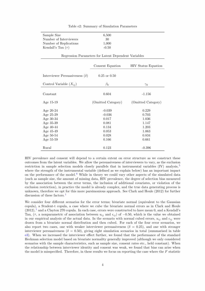
Table e2: Summary of Simulation Parameters

Sample Size 6,500Number of Interviewers 30Number of Replications 1,000Kendall’s Tau (τ) -0.50

Regression Parameters for Latent Dependent Variables

Consent Equation HIV Status Equation

Interviewer Persuasiveness (δ) 0.25 or 0.50

Control Variable (Xij) βk γk

Constant 0.604 -1.156

Age 15-19 (Omitted Category) (Omitted Category)

Age 20-24 -0.039 0.229Age 25-29 -0.036 0.703Age 30-34 0.017 1.036Age 35-39 0.081 1.147Age 40-44 0.134 1.203Age 45-49 0.053 1.063Age 50-54 0.028 0.834Age 55-59 0.166 0.661

Rural 0.123 -0.396

HIV prevalence and consent will depend to a certain extent on error structure as we construct theseoutcomes from the latent variables. We allow the persuasiveness of interviewers to vary, as the exclusionrestriction in sample selection models closely parallels that in instrumental variables (IV) analysis,5

where the strength of the instrumental variable (defined as we explain below) has an important impacton the performance of the model.6 While in theory we could vary other aspects of the simulated data(such as sample size, the amount of missing data, HIV prevalence, the degree of selection bias measuredby the association between the error terms, the inclusion of additional covariates, or violation of theexclusion restriction), in practice the model is already complex, and the true data generating process isunknown, therefore we opt for this more parsimonious approach. See Clark and Houle (2012) for furtherdiscussion of these factors.1

We consider four different scenarios for the error terms; bivariate normal (equivalent to the Gaussiancopula), a Student-t copula, a case where we cube the bivariate normal errors as in Clark and Houle(2012),1 and a Clayton 270 copula. In each case, errors were constructed to have mean 0, and a Kendall’sTau, (τ , a nonparametric of association between uij and εij) of −0.50, which is the value we obtainedin our empirical analysis of the actual data. In the scenario with normal cubed errors, uij and εij weredrawn from a bivariate normal distribution and then cubed. For each of the four error scenarios, wealso report two cases, one with weaker interviewer persuasiveness (δ = 0.25), and one with strongerinterviewer persuasiveness (δ = 0.50), giving eight simulation scenarios in total (summarised in tablee3). When we increased the interviewer effect further, we found that the performance of the standardHeckman selection model based on bivariate normality generally improved (although we only consideredscenarios with the sample characteristics, such as sample size, consent rates etc., held constant). Whenthe relationship between interviewer identity and consent was weak, we found that bias can arise whenthe model is misspecified. Therefore, in these results we focus on reporting the case where the F statistic

4

was close to 10 (with is a value commonly used a rule of thumb for having a weak instrument in IVanalysis).6

Table e3: Summary of the Eight Simulation Scenarios

Error Term Structure (uij , εij) Strength of Interviewer Persuasiveness (δ)

Scenario 1 Scenario 2

Gaussian Copula (Bivariate Normal) Weak (δ = 0.25) Stronger (δ = 0.50)

Student-t Copula Weak (δ = 0.25) Stronger (δ = 0.50)

Bivariate Normal Cubed Weak (δ = 0.25) Stronger (δ = 0.50)

Clayton 270 Copula Weak (δ = 0.25) Stronger (δ = 0.50)

For each of the eight simulation scenarios, we compare the mean proportional error, calculated as

mean(HIVModel −HIVTrue)

HIVTrue, for each of the following models: Gaussian (Cg), which is equivalent to the

standard bivariate normal probit model; Frank (Cf ); 90 and 270 degrees rotated Clayton (Cc90 ,Cc270); 90and 270 degrees rotated Joe (CJ90 ,CJ270); 90 and 270 degrees rotated Gumbel (CG90 ,CG270); Student-t(Ct), and an imputation-based estimate using the MICE package.7 We also considered more compleximputation approaches and found similar results. We also consider the root mean square error (RMSE),calculated as

√mean(HIVModel −HIVTrue)2, and calculate the partial F statistic for interviewer iden-

tity in the consent equation, which we obtain by implementing a linear probability model for consent onthe covariates (age category and place of residence) and interviewer identity, and running a joint test ofstatistical significance on the interviewer identity parameters. All analyses were conducted in R, version3.1,8 using the SemiParBIVProbit package.9 The following section gives the relevant R code. See themain text for a graphical representation of these copulae and further details on the implementation ofthese models. We also use the following other R packages in the analysis and to generate this document:aod,10 CDVine,11 copula,12 doParallel,13 doRNG,14 foreach,15 and knitr.16

Results

We summarize our findings in table e4, which compares the results from the standard Heckman-typeselection model (using the assumption of bivariate normality), the imputation model, and the preferredcopula model. For the scenarios with normal errors and normal cubed errors, the preferred copula modelis the copula with the best fit, as determined by the AIC (Akaike Information Criterion). For the otherscenarios (Student-t copula, Clayton 270 copula), the preferred copula for comparison is the underlyingtrue model. In the first two error scenarios (normal errors and Student-t errors) the standard Heckmanselection model performs well, however bias emerges in the next two error scenarios (normal cubed errorsand Clayton 270 errors). For example, when the normal errors are cubed and the F statistic is around3.5 we find that the mean bias of the standard Heckman model is -14%. In contrast, our copula modelgives a mean bias of -6% in this scenario, and the associated RMSE is also lower at 0.029 compared to0.042 for the standard bivariate normal model. The sampling distribution of the two estimators in thiscase, along with the imputation model, is shown in figure 2 in the main text. In addition, the meanbias for the bivariate normal model in the case with Clayton 270 errors and an F statistic of 6.8 is 12%compared to -2.7% for the copula model. Likewise the RMSE is also larger for the normal model in thiscase (0.039 compared to 0 029). It is important to note that the imputation model performs poorly inall cases (bias of 40% to 50%).

While some minimal bias may remain in some cases in the copula models, this simulation analysisdemonstrates that they are still preferable to the default normal model in the cases we examined. For

5

example, a mean bias of -6% for the copula model in the scenario with normal cubed errors correspondsto a mean HIV prevalence estimate of 19.6%, compared to true mean prevalence of 20.8%, mean observedHIV prevalence of 11.7%, mean imputed HIV prevalence of 11.9%, and a mean bivariate normal selectionmodel HIV prevalence estimate of 17.9%. The bias of the copula model is thus less than half that ofthe standard Heckman model. In addition, the copula model is more efficient. However, there areimportant directions for future research. As in Clark and Houle (2012),1 we find some scenarios can stillresult in convergence failures. Here, we exclude them from the analysis. Work is ongoing to improvethe implementation of these models. We only considered a limited number of scenarios, and factorssuch as sample size and amount of missing data could have an impact on the relative performance ofcopula models. Similarly, alternative specifications with additional covariates and potential interactionscould also affect results, but this is difficult to assess given our limited knowledge about the true datagenerating process. In practice, violation of the exclusion restriction (which would occur if intervieweridentity was associated with HIV status) is likely to impact on the model performance,17 however weonly considered cases where this assumption was valid by construction. Finally, we choose the preferredcopula model on the basis of conventional information criteria. However, the literature on copula modelselection for censored data is underdeveloped, and the implementation of more appropriate goodness offit tests could substantially improve the performance of copula models in future applications.

6

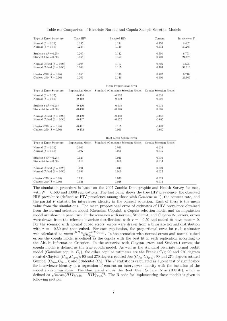
Table e4: Comparison of Bivariate Normal and Copula Sample Selection Models

Type of Error Structure True HIV Selected HIV Consent Interviewer F

Normal (δ = 0.25) 0.235 0.134 0.750 8.407Normal (δ = 0.50) 0.235 0.139 0.733 30.200

Student-t (δ = 0.25) 0.265 0.142 0.701 6.751Student-t (δ = 0.50) 0.265 0.152 0.700 24.978

Normal Cubed (δ = 0.25) 0.208 0.117 0.805 3.525Normal Cubed (δ = 0.50) 0.208 0.115 0.763 32.213

Clayton-270 (δ = 0.25) 0.265 0.136 0.702 6.716Clayton-270 (δ = 0.50) 0.265 0.146 0.700 24.905

Mean Proportional Error

Type of Error Structure Imputation Model Standard (Gaussian) Selection Model Copula Selection Model

Normal (δ = 0.25) -0.434 -0.002 0.010Normal (δ = 0.50) -0.412 -0.002 0.001

Student-t (δ = 0.25) -0.470 -0.018 0.015Student-t (δ = 0.50) -0.430 -0.026 0.006

Normal Cubed (δ = 0.25) -0.439 -0.138 -0.060Normal Cubed (δ = 0.50) -0.447 -0.052 -0.085

Clayton-270 (δ = 0.25) -0.491 0.115 -0.027Clayton-270 (δ = 0.50) -0.452 0.091 -0.007

Root Mean Square Error

Type of Error Structure Imputation Model Standard (Gaussian) Selection Model Copula Selection Model

Normal (δ = 0.25) 0.102 0.021 0.024Normal (δ = 0.50) 0.097 0.011 0.015

Student-t (δ = 0.25) 0.125 0.031 0.030Student-t (δ = 0.50) 0.114 0.016 0.014

Normal Cubed (δ = 0.25) 0.091 0.042 0.029Normal Cubed (δ = 0.50) 0.093 0.019 0.022

Clayton-270 (δ = 0.25) 0.130 0.039 0.029Clayton-270 (δ = 0.50) 0.121 0.028 0.013

The simulation procedure is based on the 2007 Zambia Demographic and Health Survey for men,with N = 6, 500 and 1,000 replications. The first panel shows the true HIV prevalence, the observedHIV prevalence (defined as HIV prevalence among those with Consent = 1), the consent rate, andthe partial F statistic for interviewer identity in the consent equation. Each of these is the meanvalue from the simulations. The mean proportional error of estimates of HIV prevalence obtainedfrom the normal selection model (Gaussian Copula), a Copula selection model and an imputationmodel are shown in panel two. In the scenarios with normal, Student-t, and Clayton 270 errors, errorswere drawn from the relevant bivariate distributions with τ = −0.50 and scaled to have mean= 0.For the scenario with normal cubed errors, errors were drawn from a bivariate normal distributionwith τ = −0.50 and then cubed. For each replication, the proportional error for each estimator

was calculated as mean (HIVModel−HIVTrue)HIVTrue

. In the scenarios with normal errors and normal cubederrors the copula model is defined as the copula with the best fit in each replication according tothe Akaike Information Criterion. In the scenarios with Clayton errors and Student-t errors, thecopula model is defined as the true copula model. As well as the standard bivariate normal probitmodel (Gaussian copula, Cg), the other copulae estimates are the Frank (Cf ); 90 and 270 degreesrotated Clayton (Cc90 ,Cc270); 90 and 270 degrees rotated Joe (CJ90 ,CJ270); 90 and 270 degrees rotatedGumbel (CG90

,CG270); and Student-t (Ct). The F statistic is calculated as a joint test of significance

for interviewer identity in a regression of consent on interviewer identity with the inclusion of themodel control variables. The third panel shows the Root Mean Square Error (RMSE), which isdefined as

√mean(HIVModel −HIVTrue)2. The R code for implementing these models is given in

following section.

7

eAppendix References

[1] S.J. Clark and B. Houle. Evaluation of heckman selection model method for correcting estimatesof HIV prevalence from sample surveys via realistic simulation. Center for Statistics and the SocialSciences Working Paper No. 120, University of Washington, 2012.

[2] Jeffrey A Dubin and Douglas Rivers. Selection bias in linear regression, logit and probit models.Sociological Methods & Research, 18(2-3):360–390, 1989. ISSN 0049-1241.

[3] James J Heckman. Sample selection bias as a specification error. Econometrica: Journal of theeconometric society, pages 153–161, 1979. ISSN 0012-9682.

[4] Wynand PMM Van de Ven and Bernard Van Praag. The demand for deductibles in private healthinsurance: A probit model with sample selection. Journal of econometrics, 17(2):229–252, 1981.ISSN 0304-4076.

[5] Edward Vytlacil. Independence, monotonicity, and latent index models: An equivalence result.Econometrica, 70(1):331–341, 2002.

[6] James H Stock, Jonathan H Wright, and Motohiro Yogo. A survey of weak instruments and weakidentification in generalized method of moments. Journal of Business & Economic Statistics, 20(4),2002.

[7] Stef Buuren and Karin Groothuis-Oudshoorn. MICE: Multivariate imputation by chained equationsin r. Journal of statistical software, 45(3), 2011. ISSN 1548-7660.

[8] R Development Core Team. R: A Language and Environment for Statistical Computing. R Foun-dation for Statistical Computing, Vienna, Austria, 2014. URL http://www.R-project.org. ISBN3-900051-07-0.

[9] Giampiero Marra and Rosalba Radice. SemiParBIVProbit: Semiparametric bivariate probit mod-elling. R package version 3.2-12, 2014.

[10] Matthieu Lesnoff and Renaud Lancelot. Aod: analysis of overdispersed data. R package version, 1,2012.

[11] Eike Christian Brechmann and Ulf Schepsmeier. Modeling dependence with c-and d-vine copulas:The r-package cdvine. Journal of Statistical Software, 52(3):1–27, 2013.

[12] Jun Yan. Enjoy the joy of copulas: with a package copula. Journal of Statistical Software, 21(4):1–21, 2007.

[13] Revolution Analytics and Steve Weston. doparallel: Foreach parallel adaptor for the parallel package.R package version, 1(8), 2014.

[14] Renaud Gaujoux. dorng: Generic reproducible parallel backend for foreach loops. R package version,1(6), 2014.

[15] Revolution Analytics. foreach: Foreach looping construct for r. R package version, 1, 2013.

[16] Yihui Xie. knitr: A general-purpose package for dynamic report generation in r. R package version,1(7), 2013.

[17] David Madden. Sample selection versus two-part models revisited: the case of female smoking anddrinking. Journal of Health Economics, 27(2):300–307, 2008. ISSN 0167-6296.

8

http://www.R-project.org

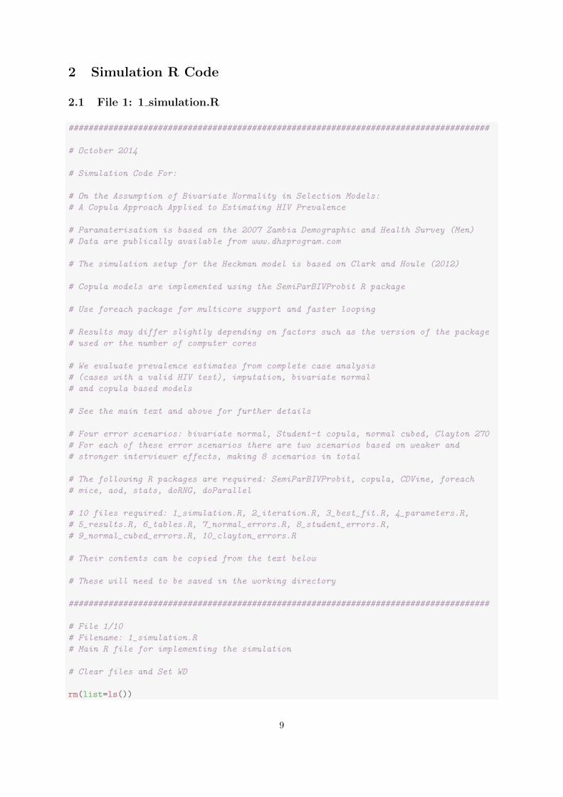
2 Simulation R Code

2.1 File 1: 1 simulation.R

#####################################################################################

# October 2014

# Simulation Code For:

# On the Assumption of Bivariate Normality in Selection Models:

# A Copula Approach Applied to Estimating HIV Prevalence

# Paramaterisation is based on the 2007 Zambia Demographic and Health Survey (Men)

# Data are publically available from www.dhsprogram.com

# The simulation setup for the Heckman model is based on Clark and Houle (2012)

# Copula models are implemented using the SemiParBIVProbit R package

# Use foreach package for multicore support and faster looping

# Results may differ slightly depending on factors such as the version of the package

# used or the number of computer cores

# We evaluate prevalence estimates from complete case analysis

# (cases with a valid HIV test), imputation, bivariate normal

# and copula based models

# See the main text and above for further details

# Four error scenarios: bivariate normal, Student-t copula, normal cubed, Clayton 270

# For each of these error scenarios there are two scenarios based on weaker and

# stronger interviewer effects, making 8 scenarios in total

# The following R packages are required: SemiParBIVProbit, copula, CDVine, foreach

# mice, aod, stats, doRNG, doParallel

# 10 files required: 1_simulation.R, 2_iteration.R, 3_best_fit.R, 4_parameters.R,

# 5_results.R, 6_tables.R, 7_normal_errors.R, 8_student_errors.R,

# 9_normal_cubed_errors.R, 10_clayton_errors.R

# Their contents can be copied from the text below

# These will need to be saved in the working directory

#####################################################################################

# File 1/10

# Filename: 1_simulation.R

# Main R file for implementing the simulation

# Clear files and Set WD

rm(list=ls())

9

# Load librarys

library(SemiParBIVProbit)

library(copula)

library(CDVine)

library(foreach)

library(mice)

library(aod)

require(stats)

library(doRNG)

library(doParallel)

setwd("C:/Users/User/Desktop/R")

# Optionally set number of processors for multicore support

cl=makeCluster(6)

registerDoParallel(cl)

# Measure run time

ptm <- proc.time()

# Load parameters for model

source("4_parameters.R")

### Scenario_1 with normal errors and weaker interviewer effects ###

# Interviewer effect

# Weaker interviewer effect with 0.25

theta10<- 0.25

# Scenario number

scenario=1

# Run simulation

source("2_iteration.R")

# Obtain best fit copula

source("3_best_fit.R")

# Generate results table

source("5_results.R")

results_1=results

# Remove results

try(rm(results))

# Optionally save results for scenario 1

save(results_1, file="normal_1.Rdata")

### Scenario_2 with normal errors and stronger interviewer effects ###


# Stronger interviewer effect with 0.5

theta10<- 0.5

10

# Scenario number

scenario=2

# Run simulation






results_2=results

# Remove results

try(rm(results))


save(results_2, file="normal_2.Rdata")

### Scenario_3 with Student-t errors and weaker interviewer effects ###



theta10<- 0.25

# Scenario number

scenario=3

# Run simulation






results_3=results

# Remove results

try(rm(results))


save(results_3, file="student_1.Rdata")

### Scenario_4 with Student-t errors and stronger interviewer effects ###



theta10<- 0.5

# Scenario number

scenario=4

11

# Run simulation






results_4=results

# Remove results

try(rm(results))


save(results_4, file="student_2.Rdata")

### Scenario_5 with normal cubed errors and weaker interviewer effects ###



theta10<- 0.25

# Scenario number

scenario=5

# Run simulation






results_5=results

# Remove results

try(rm(results))


save(results_5, file="normal_cubed_1.Rdata")

### Scenario_6 with normal cubed errors and stronger interviewer effects ###



theta10<- 0.5

# Scenario number

scenario=6

# Run simulation


12





results_6=results

# Remove results

try(rm(results))


save(results_6, file="normal_cubed_2.Rdata")

### Scenario_7 with Clayton 270 errors and weaker interviewer effects ###



theta10<- 0.25

# Scenario number

scenario=7

# Run simulation






results_7=results

# Remove results

try(rm(results))


save(results_7, file="clayton_1.Rdata")

### Scenario_8 with Clayton 270 errors and stronger interviewer effects ###



theta10<- 0.5

# Scenario number

scenario=8

# Run simulation




13



results_8=results

# Remove results

try(rm(results))


save(results_8, file="clayton_2.Rdata")

results_all=as.data.frame(rbind(results_1,results_2,results_3,results_4,results_5,

results_6,results_7,results_8))

proc.time() - ptm

# Summary tables

source("6_tables.R")

14

2.2 File 2: 2 iteration.R

# File 2/10

# Filename: 2_iteration.R

# R file for implementing the simulation iterations

# Iterate over replications

# Set seed for reproducibility with doRNG package

results<-foreach(i=1:reps, .combine='rbind', .options.RNG=123, .packages=c("copula",

"CDVine", "mice", "aod", "mvtnorm", "SemiParBIVProbit")) %dorng% {

# Empty results matrix

results0 <- rep(NA,43)

results0[43] <-scenario

### 1. First generate age and urban/rural structure ###

#####################################################

# Generate random uniform variable to bulid age structure

data<-data.frame(ID=1:N,u=runif(N)*100)

# Categorical age variable matching age bins in the Zambia data

data$agecat<-ifelse(data$u<=21.68,0, ifelse(data$u<=38.14, 2, ifelse(data$u<=53.37,

3, ifelse(data$u<=67.78, 4, ifelse(data$u<=79.07, 5, ifelse(data$u<=86.33,6,

ifelse(data$u<=92.44, 7, ifelse(data$u<=96.87, 8, ifelse(data$u<=100, 9)))))))))

data$agecat<-factor(data$agecat, labels=c("15-19","20-24","25-29","30-34","35-39",

"40-44","45-49","50-54","55-59"))

# Create urban/rural variable to be 57% rural

data$rural<-rbinom(N, 1, prob=.57)

# Create interviewer ID with 30 interviewers to match Zambia data

data$interviewID<-floor(runif(N, 1, numbergroups))

# Create effectiveness for interviewers drawn from a normal with mean=0, sd=1

effectdata<-data.frame(interviewID=1:numbergroups, effect=rnorm(numbergroups,

mean=0, sd=1))

data2<-merge(data, effectdata, by="interviewID")

### 2. Create error terms for selection and HIV equations ###

#############################################################

if (scenario==1) source("7_normal_errors.R")

if (scenario==2) source("7_normal_errors.R")

if (scenario==3) source("8_student_errors.R")

if (scenario==4) source("8_student_errors.R")

if (scenario==5) source("9_normal_cubed_errors.R")

if (scenario==6) source("9_normal_cubed_errors.R")

if (scenario==7) source("10_clayton_errors.R")

if (scenario==8) source("10_clayton_errors.R")

data3<-cbind(data2, errors)

### 3. Latent selection variable based on characteristics + parameter values ###

15

################################################################################

# Selection equation: s^* = w + theta1*(rural) + theta2-9*age_cat +

# theta10*(interviewer effectiveness) + u_select

# Latent selection variable s_k is linear prediction

data3$s_k<- w +

theta1*data3$rural +

theta2*as.numeric(data3$agecat=="20-24") +








theta10*data3$effect + data3$u_select

# Probability of selection is then pnorm(s_k)

# Binary variable indicating selection s=1 if s_k>0

data3$s<-as.numeric(data3$s_k>0)

results0[1]=mean(data3$s)

# Regression of selection on covariates

reg1=lm(s~as.factor(agecat)+rural+as.factor(interviewID), data=data3)

# Wald and F tests of interviewer coefficients

vR <- rep(0,38)

chi2=wald.test(b=coef(reg1)-vR, Sigma = vcov(reg1), Terms=c(11,12,13,14,15,16,17,18,

19,20,21,22,23,24,25,26,27,28,29,30,31,32,33,34,35,36,37,38))$result$chi2[1]

df=wald.test(b=coef(reg1)-vR, Sigma = vcov(reg1), Terms=c(11,12,13,14,15,16,17,18,

19,20,21,22,23,24,25,26,27,28,29,30,31,32,33,34,35,36,37,38))$result$chi2[2]

f=chi2/df

results0[2]=f

### 4. Latent hiv variable based on characteristics + parameter values ###

##########################################################################

# HIV equation: hiv^* = lambda + delta1*(rural) + delta2-9*age_cat

# + delta10*(interviewer effectiveness) + u_hiv

# Latent hiv variable hiv_k is linear prediction

data3$hiv_k<-lambda +

delta1*data3$rural +

delta2*as.numeric(data3$agecat=="20-24") +





16




data3$u_hiv

# Probability of HIV+ is then pnorm(hiv_k)

# Binary variable indicating selection hiv=1 if hiv_k>0

data3$hiv<-as.numeric(data3$hiv_k>0)

results0[3]=mean(data3$hiv)

### 5. New HIV variable hiv_s reflecting selection ###

######################################################

data3$hiv_s=data3$hiv

data3$hiv_s[data3$s==0]=NA

results0[4]=mean(data3$hiv_s, na.rm=T)

### 6. Imputate HIV Status Based on Age and Rural ###

######################################################

data4=subset(data3, select=c(rural,agecat,hiv_s))

mi=mice(data4, m=1)

fit=with(mi, mean(hiv_s))

results0[5] <- mean(sapply(1, function(x) complete(mi,x)$hiv_s))

### 7. Implementation of Selection Model ###

############################################

data3$interviewID=as.factor(data3$interviewID)

try(normal<-SemiParBIVProbit(list(s~rural+agecat+interviewID, hiv_s~rural+agecat),

data=data3, BivD="N", Model="BSS"))

try(frank<-SemiParBIVProbit(list(s~rural+agecat+interviewID, hiv_s~rural+agecat),

data=data3, BivD="F", Model="BSS"))

try(t3<-SemiParBIVProbit(list(s~rural+agecat+interviewID, hiv_s~rural+agecat),

data=data3, BivD="T", nu=3, Model="BSS"))

try(c90<-SemiParBIVProbit(list(s~rural+agecat+interviewID, hiv_s~rural+agecat),

data=data3, BivD="C90", Model="BSS"))

try(c270<-SemiParBIVProbit(list(s~rural+agecat+interviewID, hiv_s~rural+agecat),

data=data3, BivD="C270", Model="BSS"))

try(j90<-SemiParBIVProbit(list(s~rural+agecat+interviewID, hiv_s~rural+agecat),

data=data3, BivD="J90" , Model="BSS"))

try(j270<-SemiParBIVProbit(list(s~rural+agecat+interviewID, hiv_s~rural+agecat),

data=data3, BivD="J270", Model="BSS"))

17

try(g90<-SemiParBIVProbit(list(s~rural+agecat+interviewID, hiv_s~rural+agecat),

data=data3, BivD="G90" , Model="BSS"))

try(g270<-SemiParBIVProbit(list(s~rural+agecat+interviewID, hiv_s~rural+agecat),

data=data3, BivD="G270", Model="BSS"))

### 8. Calculate HIV Prevalence ###

###################################

# Normal

results0[6] <-try(summary(normal)$rho)

results0[7] <-try(tableRes_0(normal)[1])

results0[8] <-try(tableRes_0(normal)[4])

results0[9] <-try(BIC(normal))

results0[10] <-try(est.prev(normal)$res[2])

# Frank

results0[11] <-try(tableRes_0(frank)[1])

results0[12] <-try(tableRes_0(frank)[4])

results0[13] <-try(BIC(frank))

results0[14] <-try(est.prev(frank)$res[2])

# T3

results0[15] <-try(tableRes_0(t3)[1])

results0[16] <-try(tableRes_0(t3)[4])

results0[17] <-try(BIC(t3))

results0[18] <-try(est.prev(t3)$res[2])

# c90

results0[19] <-try(tableRes_0(c90)[1])


results0[21] <-try(BIC(c90))

results0[22] <-try(est.prev(c90)$res[2])

# C270



results0[25] <-try(BIC(c270))

results0[26] <-try(est.prev(c270)$res[2])

# J90

results0[27] <-try(tableRes_0(j90)[1])


results0[29] <-try(BIC(j90))

results0[30] <-try(est.prev(j90)$res[2])

# J270



results0[33] <-try(BIC(j270))

results0[34] <-try(est.prev(j270)$res[2])

# G90

results0[35] <-try(tableRes_0(g90)[1])

18


results0[37] <-try(BIC(g90))

results0[38] <-try(est.prev(g90)$res[2])

# G270



results0[41] <-try(BIC(g270))

results0[42] <-try(est.prev(g270)$res[2])

# Remove objects to prevent use after non-convergence

rm(data, data2, data3, data4, effectdata, errors, chi2, df, f,reg1, fit, mi)

try(rm(normal))

try(rm(frank))

try(rm(t3))

try(rm(c90))

try(rm(c270))

try(rm(j90))

try(rm(j270))

try(rm(g90))

try(rm(g270))

results0=as.numeric(as.character(results0))

return(results0)

}

row.names(results)=NULL

results <- data.frame(results)

names(results)=c("Consent Rate", "Interviewer F Test", "True HIV Prevalence",

"Selected HIV Prevalence", "Imputed HIV Prevalence", "Normal RHO", "Normal Tau",

"Normal AIC", "Normal BIC", "Normal Model HIV Prevalence", "F Tau", "F AIC",

"F BIC", "F Model HIV Prevalence", "T Tau", "T AIC", "T BIC",

"T Model HIV Prevalence","C90 Tau", "C90 AIC", "C90 BIC", "C90 Model HIV Prevalence",

"C270 Tau", "C270 AIC", "C270 BIC", "C270 Model HIV Prevalence", "J90 Tau",

"J90 AIC", "J90 BIC", "J90 Model HIV Prevalence","J270 Tau", "J270 AIC",

"J270 BIC", "J270 Model HIV Prevalence","G90 Tau", "G90 AIC", "G90 BIC",

"G90 Model HIV Prevalence", "G270 Tau", "G270 AIC", "G270 BIC",

"G270 Model HIV Prevalence", "Simulation Type")

19

2.3 File 3: 3 best fit.R

# File 3/10

# Filename: 3_best_fit.R

# R file for extracting the copula model with the best fit according to the AIC

# Obtain Best Fit Copula

names(results)=c("consent","int_f", "hiv", "hiv_s","hiv_imp", "rho", "tau", "aic_n",

"bic_n", "hiv_n", "tau_f", "aic_f", "bic_f", "hiv_f","tau_t", "aic_t", "bic_t",

"hiv_t", "tau_c90", "aic_c90", "bic_c90", "hiv_c90","tau_c270", "aic_c270",

"bic_c270", "hiv_c270", "tau_j90", "aic_j90", "bic_j90", "hiv_j90","tau_j270",

"aic_j270", "bic_j270", "hiv_j270", "tau_g90", "aic_g90", "bic_g90", "hiv_g90",

"tau_g270", "aic_g270", "bic_g270", "hiv_g270", "sim_type")

results.mini<-results[,c("aic_n","aic_f","aic_t", "aic_c90", "aic_c270", "aic_j90",

"aic_j270", "aic_g90", "aic_g270")]

# Correct for Missing Values

results.mini[[1]][is.na(results.mini[[1]])]=999

# Best Fit is model with lowest AIC

results.mini$col.min<-apply(results.mini, 1, which.min)

results.hiv<-results[,c("hiv_n", "hiv_f", "hiv_t", "hiv_c90", "hiv_c270", "hiv_j90",

"hiv_j270", "hiv_g90", "hiv_g270")]

results.hiv<-cbind(results.hiv, results.mini$col.min)

names(results.hiv)[10]="min"

for(i in 1:reps) {results.hiv$best[i]<-results.hiv[i,results.hiv$min[i]]

}

results<-cbind(results, results.hiv$best)

results[[44]][results[[44]]==999]=NA

names(results)=c("consent","int_f", "hiv", "hiv_s","hiv_imp", "rho", "tau", "aic_n",

"bic_n", "hiv_n", "tau_f", "aic_f", "bic_f", "hiv_f","tau_t",

"aic_t", "bic_t", "hiv_t", "tau_c90", "aic_c90", "bic_c90", "hiv_c90",

"tau_c270", "aic_c270", "bic_c270", "hiv_c270", "tau_j90", "aic_j90",

"bic_j90", "hiv_j90","tau_j270", "aic_j270", "bic_j270", "hiv_j270",

"tau_g90", "aic_g90", "bic_g90", "hiv_g90","tau_g270", "aic_g270",

"bic_g270", "hiv_g270", "sim_type", "hiv_best")

20

2.4 File 4: 4 parameters.R

# File 4/10

# Filename: 4_parameters.R

# R file for loading simulation parameter values

# Number of replications

reps=1000

# Set up dataset N

N<-6500

# Create interviewer ID with 30 interviewers

numbergroups<-30

# Regression parameters were obtained from a bivariate probit model for

# Zambia DHS 2007 (Men)

# Parameters for Consent Equation

# Constant

w<-.604

# Rural effect

theta1<- .123

# Parameters for age category effects

theta2<- -.025

theta3<- -.023

theta4<- .031

theta5<- .101

theta6<- .148

theta7<- .047

theta8<- .035

theta9<- .154

# Set Parameters for HIV Equation

# Constant

lambda<- -1.156

# Rural Effect

delta1<- -.396

# Parameters for age category effects

delta2<- .229

delta3<- .703

delta4<-1.036

delta5<-1.147

delta6<-1.203

delta7<-1.063

delta8<- .834

delta9<- .661

### Summary Table Function

21

tableRes_0 <- function(object1){

summ <- summary(object1)

round(cbind(summ$KeT,summ$CIkt[1],summ$CIkt[2],

AIC(object1) ),2)

}

22

2.5 File 5: 5 results.R

# File 5/10

# Filename: 5_results.R

# R file for extracting results

# Calcualte mean proportional error and root mean square error

# Error

results$hiv_n1_e=(results$hiv_n-results$hiv)

results$hiv_imp1_e=(results$hiv_imp-results$hiv)

results$hiv_best1_e=(results$hiv_best-results$hiv)

results$hiv_c2701_e=(results$hiv_c270-results$hiv)

results$hiv_t1_e=(results$hiv_t-results$hiv)

# Proportional Error

results$hiv_n1=(results$hiv_n-results$hiv)/results$hiv

results$hiv_imp1=(results$hiv_imp-results$hiv)/results$hiv

results$hiv_best1=(results$hiv_best-results$hiv)/results$hiv

results$hiv_c2701=(results$hiv_c270-results$hiv)/results$hiv

results$hiv_t1=(results$hiv_t-results$hiv)/results$hiv

# RMSE

# Root Mean Square Error

results$hiv_n1_rmse=sqrt(mean(results$hiv_n1_e^2, na.rm=T))

results$hiv_imp1_rmse=sqrt(mean(results$hiv_imp1_e^2, na.rm=T))

results$hiv_best1_rmse=sqrt(mean(results$hiv_best1_e^2, na.rm=T))

results$hiv_c2701_rmse=sqrt(mean(results$hiv_c2701_e^2, na.rm=T))

results$hiv_t1_rmse=sqrt(mean(results$hiv_t1_e^2, na.rm=T))

23

2.6 File 6: 6 tables.R

# File 6/10

# Filename: 6_tables.R

# R file for preparing tables

# Results tables

# New variable for copula model


results_all$hiv_copula1=NA

results_all$hiv_copula1[results_all$sim_type %in% 1]=

results_all$hiv_best1[results_all$sim_type %in% 1]




results_all$hiv_t1[results_all$sim_type %in% 3]


results_all$hiv_t1[results_all$sim_type %in% 4]






results_all$hiv_c2701[results_all$sim_type %in% 7]


results_all$hiv_c2701[results_all$sim_type %in% 8]


results_all$hiv_copula_rmse=NA

results_all$hiv_copula_rmse[results_all$sim_type %in% 1]=

results_all$hiv_best1_rmse[results_all$sim_type %in% 1]




results_all$hiv_t1_rmse[results_all$sim_type %in% 3]


results_all$hiv_t1_rmse[results_all$sim_type %in% 4]



24




results_all$hiv_c2701_rmse[results_all$sim_type %in% 7]


results_all$hiv_c2701_rmse[results_all$sim_type %in% 8]

# Table 1 Summary Statistics

table1=cbind(aggregate(results_all$hiv,by=list(results_all$sim_type),

FUN=mean, na.rm=TRUE),

aggregate(results_all$hiv_s,by=list(results_all$sim_type),


aggregate(results_all$consent,by=list(results_all$sim_type),


aggregate(results_all$int_f,by=list(results_all$sim_type),

FUN=mean, na.rm=TRUE))

table1=round(table1[c(2,4,6,8)],3)

names(table1)=c("True HIV Prevalence (%)", "Observed HIV Prevalence (%)",

"Consent (%)", "Interviewer F")

rownames(table1)=c("Normal: Weaker Interviewer Effects",

"Normal: Stronger Interviewer Effects",

"Student-t: Weaker Interviewer Effects", "Student-t: Stronger Interviewer Effects",

"Normal Cubed: Weaker Interviewer Effects",

"Normal Cubed: Stronger Interviewer Effects", "Clayton-270: Weaker Interviewer Effects",

"Clayton-270: Stronger Interviewer Effects")

# Table 2 Mean Proportional Error

table2=cbind(aggregate(results_all$hiv_imp1,by=list(results_all$sim_type),


aggregate(results_all$hiv_n1,by=list(results_all$sim_type),


aggregate(results_all$hiv_copula1,by=list(results_all$sim_type),


table2=round(table2[c(2,4,6)],3)

names(table2)=c("Imputation Model", "Standard (Gaussian) Selection Model",

"Copula Selection Model")



"Student-t: Weaker Interviewer Effects",

"Student-t: Stronger Interviewer Effects",


"Normal Cubed: Stronger Interviewer Effects",

"Clayton-270: Weaker Interviewer Effects",


25

# Table 3 Root Mean Square Error

table3=cbind(aggregate(results_all$hiv_imp1_rmse,by=list(results_all$sim_type),


aggregate(results_all$hiv_n1_rmse,by=list(results_all$sim_type),


aggregate(results_all$hiv_copula_rmse,by=list(results_all$sim_type),


table3=round(table3[c(2,4,6)],3)

names(table3)=c("Imputation Model", "Standard (Gaussian) Selection Model",

"Copula Selection Model")



"Student-t: Weaker Interviewer Effects",

"Student-t: Stronger Interviewer Effects",


"Normal Cubed: Stronger Interviewer Effects",

"Clayton-270: Weaker Interviewer Effects",


26

2.7 File 7: 7 normal errors.R

# File 7/10

# Filename: 7_normal_cubed_errors.R

# R file for drawing bivariate normal cubed errors

# Matrix for Error Terms

rho=-0.75

mu1=c(0,0)

Sigma<-matrix(data=c(1, rho, rho, 1), nrow=2, ncol=2)



### Normal Errors

errors<-as.data.frame(mvrnorm(N, mu=mu1, Sigma))

names(errors)<-c("u_select", "u_hiv")

27

2.8 File 8: 8 student errors.R

# File 8/10

# Filename: 8_student_errors.R

# R file for drawing errors from Student-t



### Student-t Errors

clay.cop.6 = tCopula(0.75, dim=2, df=4)

tau(clay.cop.6)

errors=as.data.frame(rCopula(N, clay.cop.6))


errors$u_select=errors$u_select-mean(errors$u_select)

errors$u_select=errors$u_select/sd(errors$u_select)

errors$u_hiv=errors$u_hiv-mean(errors$u_hiv)

errors$u_hiv=errors$u_hiv/sd(errors$u_hiv)

errors$u_hiv=-errors$u_hiv

28

2.9 File 9: 9 normal cubed.R

# File 9/10

# Filename: 9_normal_cubed.R

# R file for drawing errors from normal cubed

# Matrix for Error Terms

rho=-0.75

mu1=c(0,0)

Sigma<-matrix(data=c(1, rho, rho, 1), nrow=2, ncol=2)



### Normal Cubed Errors

errors<-as.data.frame(mvrnorm(N, mu=mu1, Sigma))


# Replace Errors with Errors Squared

errors$u_select=(errors$u_select^3)

errors$u_hiv=(errors$u_hiv^3)

29

2.10 File 10: 10 clayton errors.R

# File 10/10

# Filename: 10_clayton_errors.R

# R file for drawing errors from Clayton 270



# Clayton Errors

clay.cop.6 = archmCopula(family="clayton", dim=2, param=4)

tau(clay.cop.6)

errors=as.data.frame(rCopula(N, clay.cop.6))


errors$u_select=errors$u_select-mean(errors$u_select)

errors$u_select=errors$u_select/sd(errors$u_select)

errors$u_hiv=errors$u_hiv-mean(errors$u_hiv)

errors$u_hiv=errors$u_hiv/sd(errors$u_hiv)

errors$u_select=-errors$u_select

30

3 Code for Figure 2 (Drawing from Copulae)

# Copula plots for Figure 2 in the main text

library(VineCopula)

mar=c(3,3,3,7)

par(mfrow = c(2, 2),mar=c(3.1,4.1,3.1,5.1),cex.main = 1.7, cex.lab = 1, cex.axis = 1)

nf <- layout(matrix(c(1,1,2,2,3,3,4,4,5,5,6,6,0,7,7,0), 4, 4, byrow=TRUE),

respect=FALSE)

dat = BiCopSim(N = 1000, family = 5, par =BiCopTau2Par(family = 5,

tau = -0.5))

BiCopMetaContour(u1 = dat[, 1], u2 = dat[, 2], bw = 1, size = 100, levels = c(0.01,

0.05, 0.1, 0.15, 0.2), family = 5, par = BiCopTau2Par(family = 5,

tau = -0.5), margins="norm",

main = "Frank")


tau = -0.5), par2=3)



tau = -0.5), par2=3,margins="norm", main = "Student-t")

dat = BiCopSim(N = 1000, family = 23, par = BiCopTau2Par(family = 23,

tau = -0.5))



tau = -0.5), margins="norm", main = "Clayton 90 degrees")


tau = -0.5))




main = "Clayton 270 degrees")


tau = -0.5))




main = "Gumbel 90 degrees")


tau = -0.5))




main = "Gumbel 270 degrees")

dat = BiCopSim(N = 1000, family = 1, par =BiCopTau2Par(family = 1, tau = -0.5))


0.05, 0.1, 0.15, 0.2), family = 1, par = BiCopTau2Par(family = 1, tau = -0.5),

margins="norm", main = "Gaussian")

31

eAppendix: Simulation Details and R Code On the...

Documents

Transcript of eAppendix: Simulation Details and R Code On the...