ea m9r spe~ 57.4- 7A 1 0.457, In the interest of early and ... · ea m9r spe~ 57.4- 7A 1 0.457, In...
44
ea m9r 7A spe~ 57.4- 1 0.457, In the interest of early and wide :1 - /3 7 semination of Earth Resources Survey Program information and without liability for any use made thereot." (E74-10457) GROUND PATTERN ANALYSIS IN N74-21982 THE GREAT PLAINS Semiannual Progress Report, 1 Aug. 1973 - 31 Jan. 1974 (Kansas Univ. Center for Research, Inc.) Unclas 44 p HC $5.25 CSCL 08E G3/13 00457 THE UNIVERSITY OF KANSAS CENTER FOR RESEARCH, INC. 1 2385 Irving Hill Rd.- Campus West Lawrence, Kansas 66044 https://ntrs.nasa.gov/search.jsp?R=19740013869 2018-07-06T09:45:45+00:00Z
Transcript of ea m9r spe~ 57.4- 7A 1 0.457, In the interest of early and ... · ea m9r spe~ 57.4- 7A 1 0.457, In...

ea m9r 7A spe~ 57.4- 1 0.457,In the interest of early and wide :1 - /3 7semination of Earth Resources SurveyProgram information and without liabilityfor any use made thereot."
(E74-10457) GROUND PATTERN ANALYSIS IN N74-21982THE GREAT PLAINS Semiannual ProgressReport, 1 Aug. 1973 - 31 Jan. 1974(Kansas Univ. Center for Research, Inc.) Unclas44 p HC $5.25 CSCL 08E G3/13 00457
THE UNIVERSITY OF KANSAS CENTER FOR RESEARCH, INC.1 2385 Irving Hill Rd.- Campus West Lawrence, Kansas 66044
https://ntrs.nasa.gov/search.jsp?R=19740013869 2018-07-06T09:45:45+00:00Z

KANSAS ENVIRONMENTAL ANDRESOURCE STUDY: A GREAT PLAINS
MODEL
JAN UARY 1974
Type II Progress Report for thePeriod August 1, 1973 through January 31, 1974
Prepared for:
National Aeronautics and Space AdministrationGoddard Spaceflight CenterGreenbelt, Maryland 20771
Contract No. NAS 5-21822
2385 Irving Hill Rd.-CampusWest Lawrence, Kansas 66044

KANSAS ENVIRONMENTAL AND RESOURCE STUDY
A GREAT PLAINS MODEL
Ground Pattern Analysis in the Great Plains
F. T. Ulaby, Principal Investigator (Acting)University of Kansas Center for Research, Inc.Remote Sensing Laboratoryc/o Space Technology CenterNichols Hall2291 Irving Hill Drive-Campus WestLawrence, Kansas 66045
January 1974Type II Progress Report for the Period August 1,1973 through January 31, 1974Report No. 2266-9
Prepared for:
NATIONAL AERONAUTICS AND SPACE ADMINISTRATION
GODDARD SPACEFLIGHT CENTER
GREENBELT, MARYLAND 20771
Contract No. NAS 5-21822, Task 6
17T

Semi-Annual ERTS-A UserInvestigation Report
Type II Progress Reportfor the Period August 1, 1973 through January 31, 1974
NASA Contract NAS 5-21822
Title of Investigation: Ground Pattern Analysis in the Great Plains
ERTS-A Proposal No.: 60-8
Task Number: 6
Co-principle Investigators: John C. Davis and Fawwaz T. Ulaby
NASA-GSFC PI ID No.: UN 657
Report Prepared by: , , , '__
,James. L. McNaughton Dwight D. Egbert James R. McCauleyResearch Engineer Sr. Research Engineer Sr. Research Geologi.
Report Approved by: LA- S ',
Fawwaz T. UlabyCo-principle Investigator

TECHNICAL REPOrT STANDARD TITLE PAGE
1. Report No. 2. Government Accession No. i. kecplent's Catalog No.
2266-94. Tifl. .nd Aivbtp ottore
Kansas Environmental and Resource Study: A Great January1974Plains Model-Ground Pattern Analysis in the Great 6. Peforming Organization Code
Plains7. Au'or(s)ame s L. McNaughton, Dwight D. Egbert, 8. Performng Organzation Report No.
__JamesRL._McCnauey,,_and_ FowwazT U l aby 2266-99. Performing Organization Noae and Address 10. Work Unit No.
University of Kansas Center for Research, Inc.c/o Space Technology Center 11. Contract or Gront No.2291 Irving Hill Dr.-Campus West NAS 5-21822Lawrence, Kansas 66045 13. Type of Report and Period Covered
12. Sponsoring Agency Name and Address lype II Report for the PeriodNational Aeronautics and Space Administration August 1, 1973-January 31Goddard Space Flight Center 1974Greenbelt, Maryland 20771 14. Sponsoring Agency Code
G. R. Stonesifer, Code 43015. Supplementary Notes
None16. Abstract
The purpose of this investigation is to locate large-scale ground patternsand anomalous patterns in Kansas using ERTS-A imagery and optical data pro-cessing techniques. This report describes the spatial frequency and orienta-tional curves that were obtained for various sample areas in Kansas using ERTS-Aimagery as the input to an optical data processing system. Manual interpretatiorof the orientational curves was described in a previous report. Appropriate dataprocessing schemes were used to derive numerical parameters from these curves.These parameters are used in pattern recognition schemes to locate large-scaleground patterns and anomalous patterns in Kansas. The results reported hereindicate that spatial frequency analysis of ERTS imagery can be used to accurate-ly discriminate between large-scale ground patterns in Kansas.
L Key Words (S. lected by Author(s)) 18. Distribution StatementOptical data processingDiffraction pattern samplingSpatial frequency analysis
Large-scale geologic ground patternidentification
19. Security Cloassif. (of this report) 20. Security Classif. (of this page) 21. No. of Pages 22. Price*
Unclassified Unclassified

PREFACE
The objectives of this investigation are:
A. Mapping the surficial geology of selected sites in Kansas from
multispectral imagery, and identification of anomalous patterns;
B. Search for large-scale ground patterns by spatial frequency analysis.
An optical processing system is used in this investigation to produce ground
pattern spatial frequency and orientation information using ERTS-A imagery as input.
Interpretation of the information is done with respect to known geologic features and
other cultural and vegetation features. Appropriate data processing schemes are used
to derive numerical descriptors of these features and these descriptors, in turn,are
used in pattern recognition schemes. This investigation will then provide a mapping
technique of large-scale geologic ground patterns as well as other large-scale groundpatterns in Kansas.
The manual interpretation of the spatial frequency and orientational informationderived from the ERTS-A imagery has been completed and reported previously. Thequantitative analysis of this information is described in this report. The results des-cribed here show that spatial frequency analysis can be used to accurately discrim-inate between large-scale ground patterns.
ooIII

TABLE OF CONTENTS
Page
PREFACE iii
LIST OF FIGURES v
1.0 INTRODUCTION . . . . . . . . . . . . . . .
2.0 WORK SUMMARY . . . . . . . . . . . . . . . . . . . ...
2.1 ERTS Image Spatial Frequency Analysis . . . . . . . . 32.2 Physiographic Pattern Descriptors (Parameters) . . . . . 102.3 Classification Results and Analysis . . . . . . . . . . 20
3.0 PROGRAM FOR NEXT REPORTING PERIOD . . . . . . . . . . . 22
4.0 CONCLUSIONS .. . . . . . . . . . . . . . . . . . . . 23
5.0 RECOMMENDATIONS . . . . .......... . . . . . . 24
APPENDIX A-Geology and Physiography of Kansas . . . . . . . . . . . 25
APPENDIX B-Optical Processing System Description . . . . . . . . . . . 32
REFERENCES ................... ......... 35
iv

LIST OF FIGURES
Page
Figure 1. Physiographic Regions of Kansas (Adapted from Schoewe, 1949)with Sample Site Locations 4
Figure 2. Block Diagram of Optical Processing and Pattern RecognitionSystem 7
Figure 3. Detail of Portion of Figure 2 Enclosed in Dashed Lines 8
Figure 4. Spatial Frequency and Orientational Curves from Two SampleAreas 9
Figure 5. Modified Spatial Frequency Curve from Area A-4 11
Figure 6. Modified Spatial Frequency Curve from Area A-5 12
Figure 7. Parameter Plot Using the Parameter (R) SLOPE 2 15
Figure 8. Parameter Plot Using the Parameter (R) SLOPE 2 for the Snow-covered Sample Areas 16
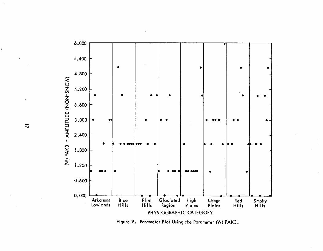
Figure 9. Parameter Plot Using the Parameter (W) PAK3 17
Figure 10. Parameter Plot Using the Parameter (R) DAVI 18
Figure 11. Parameter Plot Using the Snow-covered Sample Areas 19
Figure 12. Classification of Sample Areas in Terms of a Decision Made onthe Value of the Parameter SLOPE 2 for Each Sample Area 21
V

SECTION 1.0
INTRODUCTION
The spatial frequency analysis in this investigation involves the determination
of spatial frequency and orientational information from large-scale ground patterns
using ERTS-A imagery as the input to an optical data processing system. Previous
Type II progress reports on this investigation have described the geology and phys-
iography of Kansas, optical data processing theory, the data obtained from the op-
tical data processing of ERTS images, and the manual interpretation of these data
with respect to the geology and physiography of Kansas.
This report will concentrate on the quantitative analysis of the data obtained
from the optical data processing system. Specifically, this report will describe the
physiographic and geologic patterns that exist in Kansas, it will review the spatial
frequency and orientational information derived from ERTS-A images using the optical
data processing system, it will cover the derivation of physiographic descriptors or
parameters from these data, and it will describe the accuracy of these parameters
in predicting large-scale ground patterns and the existence of anomalous patterns
in Kansas.
To obtain more significant information from the spatial frequency analysis an
experimental design was established and has been essentially completed. The sample
areas for the experiment were methodically chosen from regions within the state whichexhibit specific geologic/physiographic characteristics. The procedure used in thisexperiment is outlined below.
A. Determine the number and extent of various geologic/physiographic
regions in Kansas from known geologic/physiographic information.
B. Select an adequate number of sample areas within each region.
C. Investigate the effect of snow cover on the ability of ERTS-A imagery
to display physiographic information. (To study this effect, equivalent
sample areas are chosen from imagery without snow cover and again
from imagery with snow cover).
D. Obtain spatial frequency characteristics from the selected sample areas.
I

E. Determine features of spatial frequency data which will allow
determination and classification of physiographic regions from
ERTS-A imagery.
F. Investigate ability of spatial frequency data to provide reliable
physiographic classification using different classification algorithms.
Following this procedure,eight regions of Kansas were chosen as most represent-
ative of certain distinctive physiographic or geologic provinces. Ten sample areas
were chosen from each of these regions. Each sample area is circular with a diameter
of approximately 23 miles. Spatial frequency data were taken twice for each of these
sample areas-once using an image when the area was snow-covered and once using
an image from the area when it was not snow-covered.
Spatial frequency and orientational curves for approximately 150 sample areas
were obtained using the optical data processing system. Appropriate data processing
schemes are used to derive numerical parameters from these curves, and these para-
meters are used as descriptors of the sample areas. These parameters may be used
then to categorize the sample areas in terms of different physiographic or geologic
provinces. The preliminary findings of the categorization experiment will be present-
ed here and the final conclusions will be presented in a later report.
2

SECTION 2.1
ERTS IMAGE SPATIAL FREQUENCY ANALYSIS
The following section is a review of the work reported in the previous Type II
ERTS-A Progress Report. This section will cover the geologic/physiographic categories
in Kansas, the spatial frequency analysis of sample areas that were chosen in each
of these categories, and the optical data processing system that was used in the spatial
frequency analysis of these sample areas. This section will also include several ex-
amples of the spatial frequency and orientational curves obtained from the optical
processor and our interpretation and analysis of them. For a full discussion of these
items refer to the Type II Progress Report for the Period February 1973-July 1973,
NASA Contract NAS5-21822.
SAMPLE SITE LOCATION
Areas of similar geologic make-up in Kansas correlate very well with the
eight physiographic regions in Figure 1. By definition, each region contains similar
landforms caused by similar geomorphic processes. In addition, each region can be
considered a geologic region since it contains outcrops of the same dominant lithology
and the same geologic age. In many cases, these regions also possess the same general
land-use. Thus the selection of sample sites for spatial frequency analysis of geologic
ground patterns was based on these eight physiographic-geologic regions.
Ten sample sites were selected for each of the eight regions and two analyses
were performed for each site, one with snow-cover and one without. The actual
dates of acquisition of the images used in this study was contingent upon cloud cover
and of course the presence of snow. As many as possible of the non-snow analyses
were performed on images recorded during the summer and early fall of 1972. The
snow-covered images were acquired during the following winter. For a few sample
sites cloud free images with snow cover were not available, thus the sample set is
not entirely complete.
3

102 1010 H-1 1000 , 990 980 970 960 95o
H_4 I I II I2 * G-3H-2 *8-4 G-1 G-20 :T 3S H-5 B-5 GLACIATED
H-3 8-1 S-1 G-4 G-5* G-6H-6 8-2 *
-- 3 G-7 REGIONS-6 F-3 * G-8B-6 * * G-9- 8-7 F-1HIGH PLAINS - S-2 F * F-7 G-10
H-7 8-8 S-7 S-3 F-2e F-4 - 399H-7 OS-9 0-10 0-2B-9 8-10 OS-F -8 0-2
* o- ~ SMOKY HILLS F-8H-8 -10 S-5 F-5
S-8 * * 0-45-4 F-9 O-3
BLUE HILLS RKANSAS A-1 F-6oH-9 VALLEY LOWLANDSF-10
A-4 A FLINT HILLS OSAGE PLAINS -38o• A-6*A-7 A-5 A-8
A-20 0-7HIGH PLAINS A-3
SR-l* R-40 A-9 -5H-10 R-7 *
,R-10 O-8R-20 R-5, REDHILLS A-10 0-6* 0-9
1 I "R-8
R-6 *R-9 O-10
0 100 Miles
Figure 1. Physiographic Regions of Kansas (Adopted from Schoewe, 1949) with Sample Site Locations.

The size of the area analyzed at each site is approximately 23 statute milesin diameter and the spacing of the sites was controlled by the size of the geologicregion. Smaller regions such as the Glaciated Region were almost completely sampled;in larger regions, the sampling was more scattered. Also some sample sites crossover into neighboring states but remain in the same geologic region.
For all sample sites except one, MSS 5 images were used in the analysis. Thisband was judged to contain the most information pertinent to the investigation. Thelone exception is a sample site in northwest Kansas where all four MSS bands wereavailable for analysis. This site contains an area of well-developed parallel drain-age and all four bands were analyzed to determine the relative merits of each band.
Sample site center points are plotted in Figure 1 and each site has an alpha-numeric identifier. The letter refers to the geologic region in which the sample siteoccurs and the numbers identify the ten sample sites in that region. A snow-coveredsample is assigned a number that is ten more than its non-snow counter part. Thus-in the case of "0-6" for instance, "0" refers to the Osage Plains region, "6" refersto the sixth sample site; "0-16" refers to the same sample site that occurs on a snow-covered image. The curves that result from the analysis of these samples are giventhe same designations. The sample site in the High Plains region which is analyzedon all four MSS bands is designated "M" in Figure 1.
Detailed analysis of each sample site was performed and the results of thisanalysis were presented in the previous Type II reporton this investigation. For adiscussion of the physiography and geology of Kansas see Appendix A.
FREQUENCY DECOMPOSITION OF SAMPLE AREAS
Each sample area on the ERTS image is composed of ground patterns of charac-teristic spatial frequencies and orientations. The spatial frequencies here refer tovariations of density on the image as a function of distance. Hence, if we decom-pose the image sample area into its component frequencies and plot their intensity;and if we plot the "strength" of preferred orientations in the image versus angle,we have described the sample areaby a set of numbers. The purpose of the quanti-tative phase of this investigation is to determine how accurately this may be done.
5

The optical data processing system used in this investigation accomplishes
this decomposition of the sample area into a set of numbers which describe the spatial
spectrum of the sample area and indicates the "preferred" orientations of the large-
scale ground patterns. (For a more detailed discussion of the theory involved in
optical data processing of images see the previous Type II Progress Report on thisinvestigation.)
Each of the sample areas on the ERTS images is used as the input to an opticaldata processing system. The complete system was described in the previous Type IIreport and Appendix B contains a short description of the system. A block diagramof the optical data processing system along with the pattern recognition portion ofthe system is shown in Figure 2. Figure 3 expands on the part of Figure 2 enclosedin dashed lines.
Using this optical processor, spatial frequency and orientational curves arederived for each sample area. Examples of these curves for a few sample areas arepresented in Figure 4. The interpretation below the curves refers to the orientationalcurve. The spatialfrequency curve in each case is the staircase-type curve thatfalls off in amplitude at higher frequencies. The curve that fluctuates significantlyin amplitude is the orientational curve.
The manual interpretation of the orientational curves indicated that this analysisproduced a valid characterization of the orientation of stream patterns and otherfeatures.
6

DIFFRACTION DIFFRACTIONERTS OPTICAL PATTERNPATTERN
IMAGE SYSTEM PATTERN SAMPLING(FOURIER UNIT
TRANSFORM) (DPSU)
----------------------------------------------------
ORIENTATIONPATTERN
PHYSIOGRAPHIC CLASSIFICATION FEATURE ORIENTATION& SPATIALDESCRIPTOR -o-CATEGORY ALGORITHM S.FREQUENCY FREQUENCY
(PARAMETERS) . DATA INFORMATION
FEATURE_EN HANCEMENrT._ --- -_s_
Figure 2. Block diagram of optical processing and pattern recognition slstem.

PATTERNORIENTATION
& SPATIALFREQUENCY
INFORMATION
SPATIAL FREQ. (RING) ORIENTATION (WEDGE) DATA
DIVIDE BY MULTIPLY BYCORRESPONDING CORRESPONDINGRING AREA/ SENSITIVITYSENSITIVITY CALIBRATION
FACTOR
NORMALI ZE NORMALI ZEWITH RESPECT WITH RESPECTTO RING #1 TO LARGEST
VALUE WEDGE DATUM
TAKE RATIO(RING CURVEDIVIDED
BY AVERAGECURVE )
CALCULATEFEATURE
PARAMETERSFROM CURVE
Figure 3. Detail of portion of Fig. 2 enclosedin dashed lines.
8

A- 4 NO SNOW A - 14 SNOW1.0 >- 1.0
S0.9 0.9-
Z0.8 z.8
S0.7 0.7.N N
0.6 - 0.6
0.5- 0.5O 0Z 0.4 Z 0.4-
I II. I I l I I I
0.0 .23 .64 1.3 2.0 3.0 4.1 S. F. (lines/mi.) 0.0 .23 .64 1.3 2.0 3.0 4.125 75 125 175 ORIENT. (deg.) 25 75 125 175
A-4. Long E-W wheat fields dominate the scene resulting in a high peakat 1750. Peak at 1500 is possibly due to NE trending sandhill beltalong the Arkansas River that lacks fields.
A-14. Snow cover is light and fields still dominate the scene producing acurve similar to A-4. A peak in the spatial frequency curve is theresult of 2-3 mile wide belt of rangeland in the southern part of thearea.
1 .0 A - 5 NO SNOW .0 A - 15 SNOW
20.9 0.9
S0o8 - 0.8
r 0.7 r 0.7N N
O0.5 - 0.5O OZ 0.4 Z 0.4
0.0 .23 .64 1.3 2.0 3.0 4.1 S. F. (lines/mi.) 0.0 .23 .64 1.3 2.0 3.0 4.125 75 125 175 ORIENT. (deg.) 25 75 125 175
A-5. Long E-W fields again prevail producing a curve with a high peakat 1800. A spatial frequency peak is due to a 2 mile wide stretchof uncultivated lowlands in the northern part of the area.
A-15. Snow cover appears to accentuate field, pasture, and range patternscreating a peak at 900 in addition to the one at 1800. The peak at1100 appears to be due to N-trending drainage that is more apparenton this image.
Figure 4. Spatial frequency and orientational curvesfrom two sample areas.
9

SECTION 2.2
PHYSIOGRAPHIC PATTERN DESCRIPTORS (PARAMETERS)
This section will describe how the spatial frequency curves were modified and
how parameters which describe the features in these modified curves, as well as the
orientational curves, are derived.
The spatial frequency curves described in the last section were modified to en-
hance their ability to display features of interest. An average spatial frequency curve
was calculated for the 80 non-snow sample areas. The point by point ratio between
this curve and each individual spatial frequency curve was determined and these
values were plotted. Two of these modified curves are shown in Figures 5 and 6.
These figures show that the relative amplitudes of the various spatial frequency com-ponents are greatly emphasized. We will show in the next section that these modi-
fied spatial frequency curves characterize the sample areas very well.
FEATURE PARAMETERS
To reduce the amount of information present in the spatial frequency and orien-tational curves, various data processing schemes were developed to extract parameters
from them. These parameters describe the geologic or physiographic features givingrise to fluctuations in the curves. To determine how well these parameters characterizeeach sample area, they may be used to categorize the sample areas by using the para-meters as input to pattern classification algorithms.
For the purposes of this phase of the investigation, the range of spatial frequencieswas divided into two bands. Band 1 contains spatial frequencies between 0.0 and 1.5 lines/mile, and band 2 contains spatial frequencies between 1.7 and 4.5 lines/mile. Thisdivision essentially separates information due to high frequency fluctuations such asoccur in stream patterns in rough terrain, and low frequency information such as occurdue to field patterns. This division of frequencies appears to correspond to a naturalbreak at approximately 1.5 lines/mile.
10

SCALE FACTOR ON Y IS 1.00! 02 SCALE FACTOR ON Y IS 1.00E 00
1.375
I I I I I I I I II I I I I I I I II I I I II I I I I I I I I
1.2 ---------------- -----.-- .....----- - -- - -- - -- - -- - -------- --.... - ..... -- ----I I I I I
T I I I II I I I I I ISI I I I I
1.2te ---------.--------- - -- --- --- - --- ----- ---- ----- ---- ---- ----- ---- ---- ----- ---- ----T / I \ I I I
I/1 \i / \ I I I I..1..28 .......-.------- ! - - - ---- ~/~.~.. -I I I I I I
I I I I I I I I I
I I I I I I I
{ I II I I II I IS I I T I I I
I I - ----- - - I I I- - - - - - - - - - - -
SI I I-- -- --- ------ ----------------------------------------- - - -- ---------------
T -T --....---- -- -.-------
HI II I I I I iI I I I AI I I
I I I I I II I I I
0.08 -------- ------ . -------- "------------- .............1 T I I
I I I I I II I I I I I I III I I I I I I II I I I I I I I I
,*? -------.-- - ---.-----------------.......--......... ......... I - - ---.........-----..........
I I I I I I I II I I I I I I I
I I I I I I I I I
I I I I I I I I I
0.633 -- ------- - - - - - -- --------------------------. --. -
SI I I I I I I IT I I I I I I I I
I I I I I I I I II I I I I I I I I
0.0 .23 .64 1.3 2.0 3.0 4.1 S.F. (lines/mile)
Figure 5 . Modified spatial frequency curve from area A-4.

SC.LF FtCT~ ON Y IS i.0gc 02 SCALE FACTOR ON Y IS 1.0JE 01
I II I I I I II I I I I I I I II I I I I I I I I
I I II I I I
I T I I I I I II I I I I I T I. I I I I I II I I I I
.- - ---------- - - - - - - -.
II I I I I I III
.14s --------- --- -- -- ---. - . . - . ----- --------
I I ! I I II% I I I
H I I IT
T
VT II I I I ISI I I I II I i
I I I I I I01 . ---
---------. .........-----.... .....
TI I
I-I I I I I I I I
: iI I I I I
H *10. . - *. ..-- - -- .---------.-- --------. ......... ......... ...
8- - -. l- - -.- -
I I I I I I I
I I I I I I I I I
-o - --- -- --- -- -- --- -- -- --- -- -- -- ---------.- -... -..... ..................---- ......... -
I I I I I I I I I
I I I I I I I I I
0.0 .23 .64 1.3 2.0 3.0 4.1 S.F.(lines/mile)
Figure 6. Modified spatial frequency curve from area A-5.

Similarly, the range of orientational data was divided into four sectors-each
corresponding to 40 degrees (see Appendix B figure 2B). Sector 1 provides data on
pattern orientations that produce distributions between 25 and 65 degrees clockwise
from true north, sector 2: 65-105 degrees, sector 3: 105-145 degrees, and sector
4: 145-185 degrees.
Parameters are extracted from the spatial frequency and orientational curvesin each range.
The following parameters were calculated from the spatial frequency and orien-
tational curves for each of the bands or sectors listed above.
Orientation parameters:
DAV Average value of the curve in the 400 sector
RMSD Root Mean Square Deviation of curve from overall average in each sector
AREA A. Area of curve above overall average in sector
B. Area of curve below overall average in sector
PEAK Number of peaks or "spikes" in curve in sector
PAKS Number of data points above average in sector
Spatial frequency parameters:(These parameters are derived from the modified spatial frequency curve)
DAV Average value of the curve in each frequency band
RMSD Root Mean Square Deviation of curve from overall average in each band
AREA A. Area of curve above overall average in band
B. Area of curve below overall average in band
DARA A. Area of curve above the value 1 .0 in band
B. Area of curve below the value 1.0 in band
DYNR DYNamic Range of curve in band
SLOPE 2 A regression line is calculated for the curve in band 2 . The slope ofthis line is obtained.
13

Each parameter for all 80 non-snow and 68 snow sample areas was plotted
versus their appropriate sample area category as obtained from Figure I. Five of
these parameter plots are shown in Figures 7-11 on the following pages. Three
separate parameters are listed and two of these parameters are repeated for the 68
snow sample areas.
The notation '(R)' or '(W)' preceding the parameter name denotes the param-
eter as a spatial frequency (Ring) or Orientational (Wedge) parameter respectively.
14

1.000
0.820
0.640
0t 0.460
Z
O
Z 0.280 *00
0 00 0I 0 00 0 0 0
0 -0.26001
-0.440 -
-0.620
-0.800Arkansas Blue Flint Glaciated High Osage Red SmokyLowlands Hills Hills Region Plains Plains Hills Hills
PHYSIOGRAPHIC CATEGORY
Figure 7. Parameter Plot Using the Parameter (R) SLOPE2.

2.500
2.170
1.840 -
1.150 -
zw 1.180
0.850
0.520
0
_J 0.190
0 00 0 0
-0. 140 -* e * eI , -
-0.470
-0.800Arkansas Blue Flint Glaciated High Osage Red SmokyLowlands Hills Hills Region Plains Plains Hills Hills
PHYSIOGRAPHIC CATEGORY
Figure 8. Parameter Plot Using the Parameter (R)SLOPE2 for the Snow-covered Sample Areas.
6.000
5.400
4.800
0Z 4.200
0Z 3.600
S 2.400I
1.800
1.200
0.600
0.000 - 0 0 0 0 0Arkansas Blue Flint Glaciated High Osage Red SmokyLowlands Hills Hills Region Plains Plains Hills Hills
PHYSIOGRAPHIC CATEGORY
Figure 9. Parameter Plot Using the Parameter (W) PAK3.

3.300
2.970
2.640
0Z 2.310
O
R 1.650 -
< 0. 99
,'-, *
0.660
0.330 - * -
0.000
Arkansas Blue Flint Glaciated High Osage Red SmokyLowlands Hills Hills Region Plains Plains Hills Hills
PHYSIOGRAPHIC CATEGORYFigure 10. Parameter Plot Using the Parameter (R) DAV 1.Figure 10. Parameter Plot Using the Parameter (R) DAV1.

3.500
3.150
2.800
0 2.450Z
i 2.100 0
S1.750<I
1.400 -
S 1.050
0.700 - *-
0.350 - • * * *
0.000Arkansas Blue Flint Glaciated High Osage Red SmokyLowlands Hills Hills Region Plains Plains Hills. Hills
PHYSIOGRAPHIC CATEGORY
Figure 11. Parameter Plot Using the Snow-covered Sample Areas.

SECTION 2.3
CLASSIFICATION RESULTS AND ANALYSIS
Decision boundaries may be inserted into the parameter plots shown in thelast section based on the distribution of the amplitudes of the'parameter. If thereis a clear relationship between the amplitude of the parameter and the physiographiccharacteristics of the sample area, then this decision boundary will discriminatebetween 2 large-scale physiographic ground patterns.
This was done for the parameter labelled SLOPE2 and the results of this schemeare shown in Figure 7. As mentioned previously, SLOPE2 is merely the slope of theregression line for the modified spatial frequency curve for the frequencies in band 2.As can be seen from the plot showing the parameter SLOPE 2(Figure 7),a decision boundarymay be inserted at approximately zero slope which effectively separates the variouscategories. Sample areas from categories of relatively high spatial frequency content(Flint Hills, Red Hills, Smoky Hills) yield a positive slope, whereas sample areasfrom the other categories yield a negative value of this parameter.
This identification experiment resulted in an accuracy of 92.5% with only6 incorrect identifications based on the original categorization of the sample areas.Sample sites represented by a square were identified as belonging to the categorycomprising the Flint Hills, Red Hills, and Smoky Hills; sample sites represented bya triangle were identified as belonging to the category comprising the ArkansasValley Lowlands, High Plains, Osage Plains, Blue Hillsand the Glaciated Region.
20

1020 1010 H-1 100 990 98° 970 960 95°
- -- -- H-4 -H-2 B-4 G- G-2
M T-5 -5 GLACIATED
H-3 B-I -2 - G-4 G- G
S3-6 F-3 -8-7 F-1 ;F 0 -
B-8 S- * S-3 F-2 F-4 - 39
7 T H FG O-S -2
S5-4 1F-9 O-
H-9 F-1000 Miles
VALLEY LOWLANDSA-4 T A-6 FLINT HILLS OSAGE PLAINS -38o
V A -7 A -2A - 5 A -
HIGH PLAINS I
A-
for each sample area.R-2; R-5r EIILLS A-10 O- -9 o Z
4-IR-8R 3 * R-9
O-10V
0 100 Miles
Figure 12. Classification of sample areas in terms of a decision made on the value of the Parameter SLOPE 2for each sample area.

SECTION 3.0
PROGRAM FOR NEXT REPORTING PERIOD
During the next reporting period this investigation will be concluded. A final
report will be issued which will include a summary of the work done on this project,
plus the results and the analysis of these results. Conclusions, based on the manual
interpretation of the spatial frequency information obtained from the optical pro-
cessing system, and based on the quantitative analysis of this information, will be
presented.
Work will continue during the next reporting period on the pattern recognition
experiment that is presently being conducted. This experiment is based on the quan-
titative information mentioned above. Using various pattern recognition algorithms,
we hope to accurately classify large-scale ground patterns and anomalous patterns
that exist in Kansas.
An experiment is also planned to determine the bands of spatial frequenciesthat contain the most information with respect to specific ground features. Additional
data from optical processing of the ERTS image sample areas will be taken using
a reduced spatial frequency scale. Using these additional data, we hope to be ableto specify which frequency bands are most significant in terms of the large-scale
ground patterns in Kansas.
22

SECTION 4.0
CONCLUSIONS
The evidence presented in this report establishes that optical data processingof ERTS-A images can be used very successfully in identifying large-scale physio-graphic patterns in Kansas. It was shown that large scale physiographic patternswere identified easily based orrthe quantitative analysis of the information derivedfrom the optical processing of the ERTS-A images.
It appears that the band of frequencies between 1.7 and 4.5 lines/mile contain
most of the information on the physiographic character of large-scale ground patterns inKansas. Further experiments will be conducted along these lines as stated in section3.0.
Major conclusions based on this investigation will be presented in the TypeIII final report due in May, 1974.
23

SECTION 5.0
RECOMMENDATIONS
The recommendation presented here is repeated from the previous Type II reporton this investigation.
We have only one recommendation concerning the NASA operation of the ERTS-A
system. This recommendation concerns the quality of reproduction of the ERTS images
we receive. Our standing order is for 70 mm negative images of MSS band 5. As
a general rule these negatives are so dense as to make reproduction in our photo-
graphic laboratory very difficult.
Because of the nature of the optical data processing system which is the coreof this investigation we require positive images of a high gamma. Thus, the normal70 mm positive images provided by NASA to ERTS users are unsatisfactory for ourstudy. This is no great probbm since we have an in house photographic laboratorycapable of such reproduction from suitable negatives. However, the 70 mm negativeswe receive from NASA Goddard are generally extremely dense.
In addition to the difficulty encountered in the reproduction of these densenegatives, it seemsthat a good portion of the dynamic range of the negative must beon the shoulder of the film's H & D curve. If this is true then the effective gammaof the negative is reduced and our attempt to produce high gamma positives is madeeven more difficult.
We would appreciate any effort on the part of NASA Goddard to improve therecording level of the 70 mm duplicate negatives.
24

APPEN DIX A
GEOLOGY AND PHYSIOGRAPHY OF KANSAS
Kansas lies within the Stable Interior, a large geologic province of North
America occupying most of the region between the Appalachians and the Rocky
Mountains. This area has suffered little in the way of intense tectcnic activity
since early Cambrian sediments were first deposited approximately 600 million years
ago. The area which is now Kansas was the site of shallow seas during a good
portion of this period. The result has been the formation and preservation of
sedimentary formations (sandstones, shales, and limestones) which cover the much
older pre-Cambrian basement rocks. The total thickness of these sedimentary rocks
is nowhere more than 9500'. This sedimentary cover is thin when compared tosedimentary thicknesses in other parts of the country where sedimentary basins may
be 20,000' to 30,000' deep.
The sedimentary formations in Kansas are relatively thin and exhibit a slight
but persistent westward dip at the surface. The present day streams and rivers of the
state flow in a generally eastward direction from the piedmont of the Rocky Mountcins
to the Missouri and Mississippi Rivers. This reflects the uplift and eastward tilling
of much of the state which occurred with the formation of the Rocky Mountains.
Thus the surface elevation of the state increases from the eastern border to the
western boundary ranging from less than 800' to more than 4,000'. In traveling
in a westward direction across the state, one not only gains elevation but crosses
the outcrops of progressively younger sedimentary rocks. Because of the westward
dip of the rock units and the subsequent erosion, they are arranged in a stairstep
fashion with each upward step representing a younger sedimentary unit.
The lithologic makeup of a rock unit, its structural attitude cnd the
weathering forces operating upon it determine the landforns that will form in the
area of its outcrop. Because of the westward dip of sedimentary rocks in Kansas,and their layer-cake arrangement, much of the surface of the state is characterized
by a series of eastward facing escarpments or cuestas. These features occur where
a relatively resistant unit (such as a limestone) crops out. Such a unit tends to
produce a landform having a steep eastern face and gentle western slope. This
gentle back slope often extends across the outcrop of an overlying, less resistant unit
25

(such as a shale) to the base of the escarpment formed by the next resistant unit.
These escarpments are dissected by the erosive effects of the many eastward flowing
streams and as a result have an irregular appearance on a map or aerial photo. But
on a larger scale they maintain a general north-south orientation which is at right
angles to the prevailing dip direction of the exposed rock units.
Lithologic differences are responsible for the various physiographic regions
generally recognized in Kansas which are shown in Figure I. In the eastern part of
the state are the Osage Plains which are made up of a series of eastward-facing
escarpments formed by outcropsof Pennsylvanian limestones and shales. The Flint
Hills are actually a large escarpment formed by outcrops of a series of chert-bearing
Permian limestones that are very resistant to erosion. The Dakota sandstone outcrops
(Cretaceous) form the Smoky Hills upland in the North Central part of the state.
Likewise, the Blue Hills are formed by outcrops of Upper Cretaceous limestones and
chalks.
Beyond the Blue Hills lie the High Plains which are formed by the accumulation
of sediments derived from the erosion of'the Rocky Mountains to the west. Numerous
aggrading streams swept eastward during the Tertiary carrying and depositing sand
and gravel and forming a vast outwash plain, that is today the present land surface.
Even younger deposits occur in the various prairies and lowlacnds associated with the
Arkansas River. Some of these areas are covered with wind blown sand in the form
of dunes, both stabilized and active. In the south-central part of the state are the
Red Hills or Cimarron breaks marking the border of the High Plains in the vicinity
of the Cimarron River, which together with its tributaries eroded into the red Permian
siltstones and shales which underlie the High Plains in that area. The extreme
northeast corner of the state was occupied by the Kansan glacier during the
Pliestocene. As a result, the landscape was resculptured to some extent and the area
was covered to varying depths by glacial deposits.
STRUCTURAL GEOLOGY
The structure of Kansas is subtle for the most part, seldom being dramatically
expressed on the surface. This should be kept in mind when considering remote
sensors as tools in mapping the geology or structure of Kansas.
26

Although faulting and folding are not intense or widespread in Kansas, joints
are. According to Billings (1942), "Joints may be defined as divisional planes
or surfaces that divide rocks and along which there has been no visible movement
parallel to the plane or surface". As Merriam (1963, p. 254) states, "Little work has
been done on jointing in Kansas, although the joints are extensively developed".
Ward (K.G.S. Bulletin 191, pt. 2) in 1968 did a study of joint patterns in the
Southern Flint Hills and he concluded, among other things, that the joint patterns
measured showed a close correlation to regional tilting and may have been produced
at the time of the tilting. He also states that, "The present drainage patterns appear
to be closely related to and may be determined by the joint pattern", (Ward 1968,
p. 21). He adds, like Merriam before him that "more work concerning midcontinent
joint systems is justified" (Ward 1968, p. 21).
Stream patterns have long been known by geologists to reflect the underlying
structures, faulting, folding and jointing. Such deformation tends to rupture
competent formations creating planes of weakness along which weathering activities
are accelerated and through which streams have a tendency to flow, taking advantage
of the destructive work already done for them. Thus, by studying topographic patirerns
in an area, insight can be gained concerning the geologic structure.
Many studies have been performed by geologist using aerial photographs
as an aid in structural analysis. Kelley (1960) mapped regional fracture systems
for a large area of the Colorado Plateau using aerial photography. Boyer and
McOwen (1964) working in Texas established a relationship between fracture
patterns observed on the ground and linear features on aerial photographs. L!kewise,in the Appalachian Plateau, Lattmcn (1958) established a correlation between
bed rock joint systems and linear features on aerial photographs. These studies
and many others like them involve the visual detection, measurements, and
evaluation of linear features or lineaments. Such studies are limited by the
interpreter's ability to detect lineaments and may be handicapped by a biased
evaluation of their significant. Spatial frequency analysis may provide a means
of detecting and measuring linear features on imagery which would not ordinary be
detected by visual means. In addition, such analysis would not be guided by any
preordained knowledge of the geologic structure, and the results would be unbiased.
The small scale of the imagery used in this study negates the detection of actual
fractures or joints on the ground. However, the layer linear features associated
with stream traces and topographic alignments can be detected and will provide
most of the information concerning geologic structure.
27

LAND USE
Land-use in Kansas is predominately devoted to agriculture. However, thetype of agriculture practiced varies across the state, due to climate, soil, landform,and availability of water. Agricultural land-use can be correlated fairly well withthe physiographic regions of Figure 1. The area east of the Flint Hills, namely theOsage Plains and the Glaciated Region, is characterized by mixed farming of thecorn belt type, with generally small fields and pastures and a variety of crops grown -
including corn, soybeans, milo, etc. Hay is an important crop in some areas of thesouthern part of this area and stock farming is a common practice. To the west liesthe Flint Hills region with its areas of bluestem prairie. It is predominately aranching area specializing in finishing out transient cattle brought in from westernand southwestern ranges. The Blue Hills and Smoky Hills are also large cattle grazingregions, especially in the rougher areas where cultivation is impractical. In thissome regard the Red Hills region of the south-central part of the state is also animportant ranching area. Much of the arable area in the western two-thirds of thestate is devoted to the raising of wheat, with the most extensive wheat growingareas in the level and fertile lowlands associated with the Arkansas River. Muchwheat is also grown on the level uplands of the High Plains and in favorable areasin the Smoky Hills and Blue Hills. However, dry farming is in common practicein the western part of Kansas, where rainfall is deficient. Dry farming involvespractices designed to catch and conserve the available moisture. Toward this end,dry forming often involves the following of fields for one or two years in orderto build up a reserve of soil moisture. Thus in any given year in the western partof the state, a sizable portion of the cultivated land will be free of planted crops.Much of the High Plains is also devoted to the grazing of cattle especially the rougherlands along streams. The southern High Plains of Kansas is an important grain
sorghum growing area.
Irrigation is important in parts of western Kansas. The largest and mostextensive area of irrigation is centered around Garden City, reaching from ScottCity southward into Meade Count), and westward along the Arkansas River. Thisarea is underlain by a sedimentary basin containing thick deposits of the TertiaryOgallala formation. This formation is largely sand and gravels derived from theRocky Mountain in Tertiary time. Its porous and permeable nature make it an excellentaquifer (water yielding formation) and it feeds the many irrigation wells in this
28

area. Several crops are grown here including corn, wheat, soybeans, alfalfa, andsugar beets. Other irrigated areas in the High Plains regions also rely on the groundwater stored in the Ogallala. The more recent deposits of alluvial material inthe valley of the Arkansas River are also important aquifers. The tell-tale signsof irrigation on areal photos are the circular fields produced by pivitol sprinklersystems. The circular fields are quite large (1/2 mile in diameter) and.are discernibleon ERTS imagery as well.
The Arkansas River valley also contains areas of sand hills. In most of theseareas, the sand hills or dunes are stabilized and covered by natural vegetation.Some areas are active however with dunes in formation and smaller areas of winderosion called blowouts. Because of the rolling topography of these sand hilltracts, many are uncultivated and used as grazing areas.
On an area basis, non-agricultural land use is, of course, secondary inKansas. The remaining land area is largely tied up in cities and towns, reservoirsand their surrounding management areas, military installations, wildlife refugesand mining areas. These land uses are largely self-explanatory. However, landuse related to mining activity requires further elaboration.
Among the minerals and rocks mined in the state are lead, zinc, coalgypsum, salt, volcanic ash, limestone, sand, gravel, and clay. In addition, thestate is an important oil and gas producer. Of these activities; salt, lead, andzinc mining is performed under ground. Most of the other products are mined byquarrying operations that are generally small in areal extent. The exception isthe procurement of coal which is done by strip mining. Large areas in southeastKansas bear the effects of strip mining in the form of long parallel mounds of dirtand rock which represent the overburden removed to reach the underlying coalseam. Lakes occupy many of these abandoned strip pits today and are used as arecreational resource in the area. The reclamation of strip mined land is animportant issue in Kansas where the practice is in use and being expanded to newareas.
GEOLOGIC PATTERNS ON ERTS IMAGERY
In satellite imagery of an area such as Kansas with low relief, subtlegeologic structure and extensive land-use, the geologic ground pattern that ismost apparent is that caused by stream patterns. Pattern and frequency of streams
29

are important indicators of the rock-type upon which they are developed. In
addition, they are strongly influenced by geologic structure. Spatial frequencyanalysis of ERTS imagery lends itself to the study of drainage patterns by detectingthose patterns which display a preferred orientation or spacing. Curves that resultfrom such analysis may contain "signatures" that are attributable to basic geologicparameters. In addition, insight may be gained concerning structural trends bydetectihg stream orientations that may be influenced by joints and other structures.Such insight would be useful since little knowledge is available concerning jointtrends in Kansas and their significance.
Use of spatial frequency analysis in the study of stream patterns should beguided by a knowledge of the manner in which stream patterns are expressed on ERTSimagery and how this expression varies from place to place in the state as a resultof changing rock-type, landuse, climate and natural vegetation.
In Kansas, stream courses are generally expressed on ERTS imagery in fourdifferent ways:
1. Riparian Vegetation
In the eastern half of the state are many stream valleys that support den:rand higher stands of vegetation than do the surrounding uplands. Cottonwoods,willows and other trees and shrubs which require large amounts of water thrive nearstreams that are perennial or contain water during much of the year. Such streamsare relatively easy to identify on ERTS-1 images with the MSS5 band giving the bestexpression. On this band, riparian vegetation generally appears much darker thansurrounding fields and grasslands. In the western half of the state the increaseddryness restricts this type of vegetation to only the major perennial streams suchas the Arkansas River and the lower Smoky Hill.
2. Pure Topographic Enhancement
Several areas in the state are largely uncultivated. For the most part,these are ranching areas that are covered with both natural and introduced grasses.Trees and shrubs are generally lacking even along streams in many of these areas.The absence of distractive patterns caused by fields and gross vegetation differencespermit the enhancement of topography by differentia I illumination of slopes ofvarying orientation. This expression can be found on images covering the KansasFlint Hills, as well as the Red Hills, Smoky Hills and dissected regions adjacentto larger streams in the High Plains.
30

Topographic Enhancement of drainage patterns has a much broader application
in the winter at times of deep snow cover. The snow has the effect of giving the
landscape more uniform reflecting properties by masking over areas of different
crop and vegetation type. As a result, slope orientation becomes more critical
in determining the amount of sunlight reflected to the ERTS-sensors. The lower
sun angle in the winter serves to further cnhance the topography. Thus an area
in which stream patterns are not normally discernible.may display them fully when
snow-covered.
3. Land-Use
Differing land-use between stream valleys and uplands can often accentate
stream patterns. This can come about in a number of ways. One involves bottom
land cultivation in an area of upland grazing and occurs in association with the
major streams in the Flint Hills and other hilly areas, where the level fertile flood
plains offer the most desirable farming areas.
Another method by which land-use reflects stream patterns occurs in the
western part of the state and is the opposite of the previously mentioned method.
It is best desplayed in the High Plains and dissected High Plains area where stream
valleys are often rough and Jack flood plains. In this case the level upland areas
offer the most ideal conditions for cultivation. The valleys which are usually too
rough or rocky for farming are used as pasture.
4. Direct Stream Expression
In some situations, the actual stream beds can be delineated on ERTS imagery.
This occurs in two ways. In the eastern portion of the state the larger streams
usually contain water throughout the year and can often be discerned on the MSS 6
and MSS 7 bands of ERTS imagery due to the low return of infrared energy from
water bodies. Thus the larger streams are often dark in comparison to the surrounding
countrysides.
In a different manner, actual stream beds in the western and south-central
part of the state are also expressed on ERTS imagery. In this situation, it is the dry
stream beds which give a distinctive appearance. These dry streams are choked with
sand, which highly reflects energy in the visible region and produces a bright
appearance on MSS 4 and MSS 5 images which contrast well with the less bright
appearance of surrounding fields and vegetation.
31

APPENDIX B
OPTICAL PROCESSING SYSTEM DESCRIPTION
In this section we will present a description of the optical processing system
used for spatial frequency analysis of the ERTS images. The optical processor has
three main elements: a laser, optics, and a Recognition Systems, Inc., Diffraction
Pattern Sampling Unit (DPSU). The system configuration is shown in Figure 1B. An
ERTS-A 70 mm positive transparency is used as the input for this system. The optical
processing system can be regarded as a two step system. First, an area of the ERTS
transparency (sample area) is illuminated by the incident laser beam. This beam is
focused by the lens (dashed lines, Figure 1B) so that the point source produced by
the spatial filter is imaged at a distance z + f in front of the lens. The resulting
light intensity distribution at this point is the optical Fourier transform or amplitude
frequency spectrum of the portion of the ERTS image illuminated by the beam. Second,
the intensity distribution (frequency spectrum) of the ERTS image is sampled by the
DPSU.
The DPSU consists of a 64 element photodiode array (shown in Figure 2B) used
to detect the light intensity incident upon each element, and electronics which
amplify and digitize the output from each diode in the array. The diode array is
composed of 32 wedge-shaped photodiodes and 32 annular ring photodiodes. The
intensity distribution across each photodiode is recorded. The data from the opticalprocessor are then used in a computer program and are calibrated, printed,and
plotted.
The spatial frequency in the transform plane is related to other system param-eters by:
s = r/dX
where s = spatial frequency in transform plane
r = distance in transform plane measured from optical axis
d = distance from image transparency to detector
X = wavelength of laser radiation = 6328 Angstroms
32

The spatial frequency obtained from this calculation is converted to ground spatial
frequency using image to ground scale. The resulting curves which are plotted by
the computer program are then I c(f) 2 or intensity vs. frequency and Ic()l 2
or intensity vs. angle. These are plotted in terms of ground spatial frequency in
cycles per mile and direction in compass degrees from north.
33

transform plane (dctctor) input plane (ERTS image)
transform lenslight beam spatial filterC laser
- 3z f f
d do-
digital display 1 - 1 1
amplifier / 64 channel switching unit f do z + f
Figure lB. System configuration
Figure 2B. Detector geometry
34

REFERENCES
Billings, M. P., (1942), Structural Geology, Prenctice-Hall, Inc., EnglewoodCliffs, New Jersey
Boyer, R. E. and J. E. McQueen, (1964), "Comparison of Mapped Rock Fracturesand Airphoto Linear Features," Photogrammetric Engineering, vol. 30,pp. 630-635.
Kelley, V. C. and J. N. Clinton, (1960), "Fracture Systems and Tectonic Elementsof the Colorado Plateau,' University of New Mexico Publication in Geology,no. 6, 104 pp.
Lattman, L. H. and R. P. Nickelson, (1958), "Photogeologic Fracture Trace Mappingin Appalacian Plateau," Am. Assoc. Petroleum GeologistsBull., vol. 42,pp. 2238-2244.
Merriam, D. F., (1963), "The Geologic History of Kansas," Kansas GeologicalSurvey Bulletin 162.
Schoewe, W. H., (1949), "The Geography of Kansas, Pt. 2, Physical Geography,"Kansas Acad. Sci. Trans., vol. 52, no. 3, pp. 261-333.
Ward, J. R., (1968), "A Study of the Joint Patterns in Gently Dipping SedimentaryRocks of South-Central Kansas," Kansas Geological Survey Bulletin 191,part 2.
35

CRINC LABORATORIES
Chemical Engineering Low Temperature Laboratory
Remote Sensing Laboratory
Flight Research Laboratory
Chemical Engineering Heat Transfer Laboratory
Nuclear Engineering Laboratory
Environmental Health Engineering Laboratory
Information Processing Laboratory
Water Resources Institute
Technology Transfer Laboratory
13o