E303: Communication Systems · 2019-11-04 · standard. Related standards: CCITT m-law, ITU-T. GSM...
52
E303: Communication Systems Professor A. Manikas Chair of Communications and Array Processing Imperial College London An Overview of Fundamentals: Principles of PCM Prof. A. Manikas (Imperial College) E303: Principles of PCM v.19 1 / 52
Transcript of E303: Communication Systems · 2019-11-04 · standard. Related standards: CCITT m-law, ITU-T. GSM...

E303: Communication Systems
Professor A. ManikasChair of Communications and Array Processing
Imperial College London
An Overview of Fundamentals: Principles of PCM
Prof. A. Manikas (Imperial College) E303: Principles of PCM v.19 1 / 52

Table of Contents1 Glossary 32 Introduction 43 PCM: Bandwidth & Bandwidth Expansion Factor 84 The Quantisation Process (output point-A2) 10
Uniform Quantisers 16Comments on Uniform Quantiser 18Non-Uniform Quantisers 21max(SNR) Non-Uniform Quantisers 23Companders (non-Uniform Quantisers) 26Compression Rules (A and mu)The 6dB Law
Differential Quantisers 34Type-1Type-2 (mse Diff Quant)Examples
5 Noise Effects in a Binary PCM 44Threshold Effects in a Binary PCM 45Threshold Point 46Comments on Threshold Effects 47
6 CCITT Standards: Differential PCM (DPCM) 487 Problems of DPCM 498 Appendix-1: Alex Reeves - the "Father of PCM" 50Prof. A. Manikas (Imperial College) E303: Principles of PCM v.19 2 / 52

Glossary
GlossaryCCITT = Comite Consultatif Internationale de Telegraphie et TelephonieThis is an international committee based in Geneva, Switzerland, thatrecommends telecommunications standards, including the audiocompression/decompression standards (codecs) and the famous V. standardsfor modem speed and compression (V.34 and so on). Although thisorganization changed its name to ITU-T (International TelecommunicationsUnion-Telecommunication), the old French name lives on.Related standards: CCITT A-law, CCITT µ-law, codec, ITU-T, V. standardsCCITT A-law = This is a CCITT-ratified audio encoding and compressiontechnique supported by Windows and Web phones. Among otherimplementations, A-law was originally intended as a phone-communicationsstandard.Related standards: CCITT µ-law, ITU-T.GSM = Groupe Speciale Mobile (Global System for Mobile Communications)This set of standards is widely used in Europe for cellular communications.The audio encoding subset of the GSM standard is best known to computerusers because its data compression and decompression techniques are alsobeing used for Web-phone communication and encoding WAV and AIFF files.Related standards: AIFF, codec, WAV
Prof. A. Manikas (Imperial College) E303: Principles of PCM v.19 3 / 52

Introduction
Introduction
Prof. A. Manikas (Imperial College) E303: Principles of PCM v.19 4 / 52

Introduction
PCM = sampled quantised values of an analogue signal aretransmitted via a sequence of codewords.
i.e. after sampling & quantisation, a Source Encoder is used to mapthe quantised levels (i.e. o/p of quantiser) to codewords of γ bits
i.e. quantised level 7→ codeword of γ bits
and, then a digital modulator is used to transmit the bits, i.e. PCMsystem
There are three popular PCM source encoders (or, in other words,quantisation-levels Encoders).
I Binary Coded Decimal (BCD) source encoderI Folded BCD source encoderI Gray Code (GC) source encoder
Prof. A. Manikas (Imperial College) E303: Principles of PCM v.19 5 / 52

Introduction
g(input) 7→ gq(output)
gq : occurs at a rate Fssamplessec
(N.B: Fs ≥ 2 · Fg )
Q = quantiser’s levels;
γ = log2(Q)bitslevel
N.B.:
codeword rate (point B)
↑γ−bit codewords
sec
= quant. levels rate
↑levelssec
= sampling rate
↑samplessec
= Fs = 2Fg (1)
Prof. A. Manikas (Imperial College) E303: Principles of PCM v.19 6 / 52

Introduction
bit rate: rb = γ↑bitslevel
Fs↑
levelssec
e.g. for Q = 16 levels then rb = 4↑γ
Fs
bitssec
(e.g. transmitted sequ. =
γ=4↓︷︸︸︷
10101100︸︷︷︸↑
γ=4
γ=4↓︷︸︸︷
1101 . . .)
versions of PCM:I Differential PCM (DPCM),PCM with differential Quant.I Delta Modulation (DM): PCM with diff. quants having 2 levelsi.e. +∆ or − ∆
↑are encoded usinga single binary digit
I Note: DM∈DPCMI Others
Prof. A. Manikas (Imperial College) E303: Principles of PCM v.19 7 / 52

PCM: Bandwidth & Bandwidth Expansion Factor
PCM: Bandwidth & Bandwidth Expansion Factorwe transmit several bits for each quantiser’s o/p level⇒ BPCM > Fg
where{BPCM denotes the channel bandwidthFg represents the message bandwidth
Definition (PCM Bandwidth)baseband bandwidth:
BPCM ≥ channel symbol rate2 Hz (2)
bandpass bandwidth:
BPCM ≥ channel symbol rate2 × 2 Hz (3)
Note that, by default, the Lower bound of the ‘baseband’bandwidthis assumed and used in this course
Prof. A. Manikas (Imperial College) E303: Principles of PCM v.19 8 / 52

PCM: Bandwidth & Bandwidth Expansion Factor
Definition (Bandwidth Expansion Factor β)
β , channel bandwidthmessage bandwidth
(4)
N.B. for Binary PCMChannel Bandwidth:
BPCM =channel symbol rate
2
=bit rate2
=γFs2= γ
↑log2 Q
FgHz
⇒ BPCM = γFg (5)
Bandwidth Expansion Factor:
BPCM = γFg ⇒BPCMFg
= γ⇒ β = γ (6)
Prof. A. Manikas (Imperial College) E303: Principles of PCM v.19 9 / 52

The Quantisation Process (output point-A2)
The Quantisation Process (output point-A2)
at point A2 :a signal discrete in amplitude and discrete in time.
The blocks up to the point A2, combined, can be considered as adiscrete information source where a discrete message at its output is a“level” selected from the output levels of the quantiser.
Prof. A. Manikas (Imperial College) E303: Principles of PCM v.19 10 / 52

The Quantisation Process (output point-A2)
DefinitionThe following mapping is called quantising
analogue samples 7→ finite set of levels
where the symbol 7→ denotes a “map”
N.B.: ADC
Prof. A. Manikas (Imperial College) E303: Principles of PCM v.19 11 / 52

The Quantisation Process (output point-A2)
quantiser parameters:
Q : number of levelsbi : input levels of the quantiser, with i = 0, 1, . . . ,Q
(b0 = lowest level): known as quantiser’s end-pointsmi : outputs levels of the quantiser
(sampled values after quantisation)with i = 1, . . . ,Q; known as output-levels
rule: connects the input of the quantiser to mi
RULE:
the sampled values g(kTs ) of an analogue signal g(t) areconverted to one of Q allowable output-levels m1,m2, . . . ,mQaccording to the rule:
g(kTs ) 7→ mi (or equivalently gq(kTs ) = mi )iff bi−1 ≤ g(kTs ) ≤ bi with b0 = −∞, bQ = +∞
Prof. A. Manikas (Imperial College) E303: Principles of PCM v.19 12 / 52

The Quantisation Process (output point-A2)
quantisation noise at each sample instance:
nq(kTs ) = gq(kTs )− gs (kTs ) (7)
If the power of the quantisation noise is small, i.e. Pnq = E{n2q(kTs )
}= small,
then the quantised signal (i.e. signal at the output of the quantiser)is a good approximation of the original signal.quality of approximation may be improved by the careful choice ofbi’s and mi’s and such as a measure of performance is optimised.e.g. measure of performance: Signal to quantisation Noise power Ratio (SNRq)
SNRq =signal power
quant. noise power =PgPnq
Prof. A. Manikas (Imperial College) E303: Principles of PCM v.19 13 / 52

The Quantisation Process (output point-A2)
N.B.: Types of Quantisation
quantisers :
uniformnon-uniform
differential ={
uniform, or non-uniform
plus a differential circuit
Transfer Function:uniform quantiser non-uniform quantiser
for signals with CF = small for signals with CF = large
Prof. A. Manikas (Imperial College) E303: Principles of PCM v.19 14 / 52

The Quantisation Process (output point-A2)
The following figure illustrates the main characteristics of different types ofquantisers
Prof. A. Manikas (Imperial College) E303: Principles of PCM v.19 15 / 52

The Quantisation Process (output point-A2) Uniform Quantisers
Uniform QuantisersN.B.:
Uniform quantisers are appropriate for uncorrelated samples
let us change our notation: gq(kTs ) to gq and g(kTs ) to gthe range of the continuous random variable g is divided into Qintervals of equal length ∆
(value of g) 7→ (midpoint of the quantising interval in which the value of g falls)
or equivalently mi =bi−1 + bi
2for i = 1, 2, . . . ,Q (8)
Prof. A. Manikas (Imperial College) E303: Principles of PCM v.19 16 / 52

The Quantisation Process (output point-A2) Uniform Quantisers
step size ∆:
∆ =bQ − b0Q
(9)
rule:
rule: gq = mi iff bi−1 < g ≤ bi where{bi = b0 + i · ∆mi =
bi−1+bi2
for i = 1, 2, . . . ,Q(10)
Prof. A. Manikas (Imperial College) E303: Principles of PCM v.19 17 / 52

The Quantisation Process (output point-A2) Comments on Uniform Quantiser
Comments on Uniform Quantiser
Since, in general, Q = large ⇒ Pgq ' Pg ≡ E{g2}
Furthermore, large Q implies that Fidelity of quantiser = ↑
gq ' g
Q = 8− 16 are just suffi cient for good intelligibility of speech;
(but quantising noise can be easily heard at the background)voice telephony: minimum 128 levels; (i.e. SNRq ' 42dB)
N.B.: 128 levels ⇒ 7-bits to represent each level⇒ transmission bandwidth = ↑
Prof. A. Manikas (Imperial College) E303: Principles of PCM v.19 18 / 52

The Quantisation Process (output point-A2) Comments on Uniform Quantiser
if
{quantiser = UNIFORM
pdf of the input signal = UNIFORMthen
SNRq = Q2 = 22γ (11)
Quantisation Noise Power Pnq :
quantisation Noise Power: Pnq =∆2
12(12)
rms value of Quant. Noise:
rms value of Quant. Noise = fixed =∆√126= f {g} (13)
∴ if g(t) = small for extended period of time
⇒ SNRq < the design value
↑this phenomenon is obvious
if the signal waveform has a large CREST FACTOR
(14)
Prof. A. Manikas (Imperial College) E303: Principles of PCM v.19 19 / 52

The Quantisation Process (output point-A2) Comments on Uniform Quantiser
SNRq as a function of the Crest Factor
Remember:
CREST FACTOR ≡ peakrms
(15)
By using variable spacing︸ ︷︷ ︸↑
small spacing near 0 andlarge spacing at the extremes
⇒ CREST FACTOR effects = ↓
I =⇒this leads to NON-UNIFORM quantisersProf. A. Manikas (Imperial College) E303: Principles of PCM v.19 20 / 52

The Quantisation Process (output point-A2) Non-Uniform Quantisers
Non-Uniform QuantisersN.B.:
Non-Uniform quantisers are (like unif. quants) appropriate for uncorrelatedsamples
step size = variable = ∆i
if pdfi/p 6= uniformthen non-uniform quants yield higher SNRq than uniform quants
rms value of nq is not constant but depends on the sampled value g(kTs ) ofg(t)
Prof. A. Manikas (Imperial College) E303: Principles of PCM v.19 21 / 52

The Quantisation Process (output point-A2) Non-Uniform Quantisers
rule: gq = mi iff bi−1 < g ≤ bi
where b0 = −∞, bQ = +∞ ∆i = bi − bi−1 = variable
example:
Prof. A. Manikas (Imperial College) E303: Principles of PCM v.19 22 / 52

The Quantisation Process (output point-A2) max(SNR) Non-Uniform Quantisers
max(SNR) Non-Uniform Quantisers
bi , mi are chosen to maximize SNRq as follows:I since Q = large ⇒ Pgq ' Pg ≡ E
{g2}⇒ SNRq = max if Pnq = min
where
Pnq =Q
∑i=1
∫ bibi−1
(g −mi )2 · pdfg · dg (16)
I Therefore:
minmi ,bi
Pnq (17)
(17) ⇐⇒
dPnqdbj
= 0dPnqdmj
= 0(18)
⇒{(bj −mj )2·pdfg (bj )− (bj −mj+1)2·pdfg (bj ) = 0 for j = 1, 2, . . . ,Q − 1−2 ·
∫ bjbj−1(g −mj )·pdfg (g) · dg = 0 for j = 1, 2, . . . ,Q
(19)
In the second branch of Equation-19 the parameter mj can be seen asthe statistical mean of the j th quantiser interval
Prof. A. Manikas (Imperial College) E303: Principles of PCM v.19 23 / 52

The Quantisation Process (output point-A2) max(SNR) Non-Uniform Quantisers
Note:
the above set of equations (i.e. (19)) cannot be solved in closedform for a general pdf. Therefore for a specific pdf an appropriatemethod is given below in a step-form:
METHOD:
1. choose a m12. calculate bi’s, mi’s3. check if mQ is the mean of the interval [bQ−1, bQ = ∞]
if yes → STOPelse → choose a new m1 and then goto step-2
Prof. A. Manikas (Imperial College) E303: Principles of PCM v.19 24 / 52

The Quantisation Process (output point-A2) max(SNR) Non-Uniform Quantisers
A SPECIAL CASEmax(SNR) Non-Uniform Quantiser of a Gaussian Input Signal
if the input signal has a Gaussian amplitude pdf, that is pdfq= N(0, σg ) then it can be proved that:
Pnq = 2.2σ2gQ−1.96
↑not easy to derive
(12)
In this case the Signal-to-quantisation Noise Ratio becomes:
SNRq =PgqPnq
=σ2g
2.2σ2gQ−1.96= 0.45Q1.96 (13)
Prof. A. Manikas (Imperial College) E303: Principles of PCM v.19 25 / 52

The Quantisation Process (output point-A2) Companders (non-Uniform Quantisers)
Companders (non-Uniform Quantisers)Their performance independent of CF
Non-unif. Quant =SAMPLE
COMPRESSION+
UNIFORM
quantisER+
SAMPLE
EXPANDER
Compressor + Expander ≡ Compander
gf7→ gc i .e. gc =f{g} :
↑means
”such that"
pdfgc = uniformf−17→ g
Prof. A. Manikas (Imperial College) E303: Principles of PCM v.19 26 / 52

The Quantisation Process (output point-A2) Companders (non-Uniform Quantisers)
Popular companders: use log compression
Prof. A. Manikas (Imperial College) E303: Principles of PCM v.19 27 / 52

The Quantisation Process (output point-A2) Companders (non-Uniform Quantisers)
Two compression rules (A-law and µ-law) which are used in PSTNand provide a SNRq independent of signal statistics are givenbelow:
µ-law (USA) A-law (Europe)
In practice{A ' 87.6µ ' 100
Prof. A. Manikas (Imperial College) E303: Principles of PCM v.19 28 / 52

The Quantisation Process (output point-A2) Companders (non-Uniform Quantisers)
Compression-Rules (PCM systems)
Definitions (The µ and A laws)
µ-law A-law
gc =ln(1+µ·| g
gmax |)ln(1+µ)
gmax gc =
A·| g
gmax |1+ln(A) · gmax 0 ≤
∥∥∥ ggmax
∥∥∥ < 1A
1+ln(A·| ggmax |)
1+ln(A) gmax 1A ≤
∥∥∥ ggmax
∥∥∥ < 1where
gc = compressor’s output signal
(i.e. input to uniform quantiser)
g = compressor’s input signal
gmax = maximum value of the signal g
Prof. A. Manikas (Imperial College) E303: Principles of PCM v.19 29 / 52

The Quantisation Process (output point-A2) Companders (non-Uniform Quantisers)
6dB Lawuniform quantisera:
SNRq = 4.77+ 6γ− 20 log(CF) dB (20)
µ-law:SNRq = 4.77+ 6γ− 20 log(ln(1+ µ)) dB (21)
A-law:SNRq = 4.77+ 6γ− 20 log(1+ lnA) dB (22)
aRemember: CF = peakrms
Prof. A. Manikas (Imperial College) E303: Principles of PCM v.19 30 / 52

The Quantisation Process (output point-A2) Companders (non-Uniform Quantisers)
Figure illustrating the main characteristics of quantisers
Prof. A. Manikas (Imperial College) E303: Principles of PCM v.19 31 / 52

The Quantisation Process (output point-A2) Companders (non-Uniform Quantisers)
COMMENTS
uniform & non-uniform quantisers:
use them when samples are uncorrelated with each other (i.e. thesequence is quantised independently of the values of the precedingsamples)
practical situation:
the sequence {g(kTs )} consists of samples which are correlated witheach other. In such a case use differential quantiser.
Prof. A. Manikas (Imperial College) E303: Principles of PCM v.19 32 / 52

The Quantisation Process (output point-A2) Companders (non-Uniform Quantisers)
ExamplesPSTN
Fs = 8kHz, Q = 28 (A = 87.6 or µ = 100), γ = 8 bits/level
i.e. bit rate: rb = Fs × γ = 8k × 8 = 64 kbits/sec
Mobile-GSM
Fs = 8kHz, Q = 213 uniform ⇒ γ = 13 bits/level,
i.e. bit rate: rb = Fs × γ = 8k × 13 = 104 kbits/sec
which, with a differential circuit, is reduced to rb = 13 kbits/sec
Prof. A. Manikas (Imperial College) E303: Principles of PCM v.19 33 / 52

The Quantisation Process (output point-A2) Differential Quantisers
Differential QuantisersN.B.:
Differential quantisers are appropriate for correlated samplesnamely they take into account the sample to sample correlation in thequantisation process;
Definition (Type-1 Diff Quant.)
Transmitter (Tx) Receiver (Rx)
input currentmessagesample
The weights w are estimated based on autocorr. function of the inputThe Tx & Rx predictors should be identical.
I Therefore, the Tx transmits also its weights to the Rx (i.e. weights w aretransmitted together with the data)
Prof. A. Manikas (Imperial College) E303: Principles of PCM v.19 34 / 52

The Quantisation Process (output point-A2) Differential Quantisers
In practice, the variable being quantised is not g(kTs ) but thevariable d(kTs )
where d(kTs ) = g(kTs )− g(kTs ) (14)
i.e.
Because d(kTs ) has small variations, to achieve a certain level ofperformance, fewer bits are required. This implies that DPCM canachieve PCM performance levels with lower bit rates.6dB law:
SNRq = 4.77+ 6γ− a in dBwhere −10dB < a < 7.77dB
(15)
Prof. A. Manikas (Imperial College) E303: Principles of PCM v.19 35 / 52

The Quantisation Process (output point-A2) Differential Quantisers
Definition (Type-2: mse Diff. Quant)the largest error reduction occurs when the differential quantiser operates on the differences
between g(kTs ) and the minimum mean square error (min-mse) estimator g(kTs ) ofg(kTs )N.B.: mse = a better quantiser but it needs more hardware
Prof. A. Manikas (Imperial College) E303: Principles of PCM v.19 36 / 52

The Quantisation Process (output point-A2) Differential Quantisers
i.e.g(kTs ) = wT g
where{g = [g((k − 1)Ts ), g((k − 2)Ts ), . . . , g((k − L)Ts )]T
w = [w1,w2, . . . ,wL]T
rule:
{choose w to minimize E
{(g(kTs )− g(kTs ))2
}. . . for the Tx
choose w to minimize E{(dq(kTs ) + g(kTs ))2
}. . . for the Rx
Prof. A. Manikas (Imperial College) E303: Principles of PCM v.19 37 / 52

The Quantisation Process (output point-A2) Differential Quantisers
Differential Quantisers: ExamplesExample (Power of d(kTs))
Consider:
At point B: The power of d(kTs ) can be found as follows:
σ2d = E{d2}
= E{g2(kTs )
}︸ ︷︷ ︸=σ2g
+ E{g2((k − 1)Ts )
}︸ ︷︷ ︸=σ2g
− 2E {g(kTs )g((k − 1)Ts )}︸ ︷︷ ︸2·Rgg (Ts )
⇓σ2d = 2 · σ2g − 2 · Rgg (Ts ) = 2 · σ2g · (1−
Rgg (Ts )σ2g
) (23)
Prof. A. Manikas (Imperial College) E303: Principles of PCM v.19 38 / 52

The Quantisation Process (output point-A2) Differential Quantisers
Example (diff. circuit: signals)
Prof. A. Manikas (Imperial College) E303: Principles of PCM v.19 39 / 52

The Quantisation Process (output point-A2) Differential Quantisers
disadvantages : unrecoverable degradation is introduced by thequantisation process.
I (Designer’s task is to keep this to a subjective acceptable level)
σ2g = Rgg (0)
Rgg (τ)σ2g
: is known as the normalized autocorrelation function
DPCM with the same No of bits/sample → generally gives betterresults than PCMwith the samenumber of bits.
Prof. A. Manikas (Imperial College) E303: Principles of PCM v.19 40 / 52

The Quantisation Process (output point-A2) Differential Quantisers
Example (mse DPCM)
assume a 4-level quantiser:I/P O/P
+5 ≤ input ≤ +255 +70 ≤ input ≤ +4 +1−4 ≤ input ≤ −1 −1−255 ≤ input ≤ −5 −7
Prof. A. Manikas (Imperial College) E303: Principles of PCM v.19 41 / 52
The Quantisation Process (output point-A2) Differential Quantisers
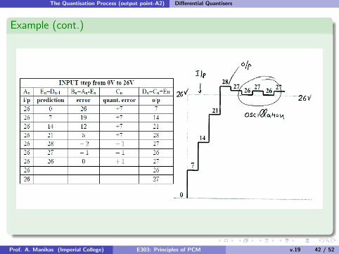
Example (cont.)
Prof. A. Manikas (Imperial College) E303: Principles of PCM v.19 42 / 52

The Quantisation Process (output point-A2) Differential Quantisers
Example (cont.)
From the last two figures we can see thatsmall variation to the i/p signal (25V ⇐⇒ 26V)
⇓large variations to o/p waveforms
Prof. A. Manikas (Imperial College) E303: Principles of PCM v.19 43 / 52

Noise Effects in a Binary PCM
Noise Effects in a Binary PCMIt can be proved that the Signal-to-Noise Ratio at the output of abinary PCM system, which employs a BCD encoder/decoder andoperates in the presence of noise, is given by the following expression
SNRout at point A of the CS-Block-Diagram on page-4
SNRout =E{g0(t)2
}E {n0(t)2}+ E {nq0(t)2}
=22γ
1+ 4 · pe · 22γ(24)
where
pe = f(type of digital modulator)
pe = T{√
(1− ρ) · EUE}
e.g. if the digital modulator is a PSK-mod. then
pe = T{√
2 · EUE}
Prof. A. Manikas (Imperial College) E303: Principles of PCM v.19 44 / 52

Noise Effects in a Binary PCM Threshold Effects in a Binary PCM
Threshold Effects in a Binary PCM
We have seen that: SNRout = 22γ
1+4·pe ·22γ
Let us examine the following two cases: SNRin = high andSNRin = low
i) SNR in = HIGH ii) SNR in = LOW
SNRin = high ⇒ pe = small SNRin = low ⇒ pe = large
⇒ 1+ 4 · pe · 22γ ' 1
⇒ SNRout = 22γ ⇒ 1+ 4 · pe · 22γ ' 4 · pe · 22γ
⇒ SNRout ' 6γ dB ⇒ SNRout ' 14·pe
Prof. A. Manikas (Imperial College) E303: Principles of PCM v.19 45 / 52

Noise Effects in a Binary PCM Threshold Point
Threshold PointDefinition (Threshold point)
Threshold point is arbitrarily defined as the SNRin at which the SNRout, i.e.
SNRout =22γ
1+ 4 · pe · 22γ
falls 1dB below the maximum SNRout(i.e. 1dB below the value 22γ).
Proof.By using the above definition it can be shown (. . . for you. . . ) that thethreshold point occurs when
pe = 116·22γ (25)
where γ is the number of bits per quant. level.
Prof. A. Manikas (Imperial College) E303: Principles of PCM v.19 46 / 52

Noise Effects in a Binary PCM Comments on Threshold Effects
Comments on Threshold Effects
Comments
The onset of threshold in PCM will result in a sudden ↑ in the output noise power.Psignal = ↑ ⇒ SNRin = ↑ ⇒ SNRout reaches 6γ dB and becomes independent of Psignal∴ above threshold: increasing signal power⇒ no further improvement in SNRoutThe limiting value of SNRout depends only on the number of bits γ perquantisation levels
Prof. A. Manikas (Imperial College) E303: Principles of PCM v.19 47 / 52

CCITT Standards: Differential PCM (DPCM)
CCITT Standards: Differential PCM (DPCM)
Definition (DPCM)
DPCM , PCM which employs a differential quantiser
i.e. DPCM reduces the correlation that often exists betweensuccessive PCM samples
The CCITT standards 32 kbitssec
DPCM The CCITT standards 64 kbitssec
DPCMspeech signal - Fg = 3.2kHz audio signal - Fg = 7kHzFs = 8 ksamplessec
Fs = 16 ksamplessec
Q = 16 levels (i.e. γ = 4 bitslevel) Q = 16 levels (i.e. γ = 4 bits
level)
Prof. A. Manikas (Imperial College) E303: Principles of PCM v.19 48 / 52

Problems of DPCM
Problems of DPCM:
1 slope overload noise:occurs when outer quantisation level is too small for large inputtransitions and has to be used repeatedly
2 “Oscillation” or granular noise:occurs when the smallest Q-level is not zero. Then, for constantinput, the coder output oscillates with amplitude equal to thesmallest Q-level.
3 “Edge Busyness” noise:occurs when repetitive edge waveform is contaminated by noise whichcauses it to be coded by different sequences of Q-levels.
Prof. A. Manikas (Imperial College) E303: Principles of PCM v.19 49 / 52

Appendix-1: Alex Reeves - the "Father of PCM"
↘↘↘↘↘↘↘↘↘↘↘↘↘↘↘↘↘↘↘↘↘↘↘↘↘↘↘↘
Prof. A. Manikas (Imperial College) E303: Principles of PCM v.19 50 / 52

Appendix-1: Alex Reeves - the "Father of PCM"
Appendix-1: Alex Reeves - the "Father of PCM"
DEEE: Introduction of the 1st ALex-Reeves Lecture in2006
"The Department of Electrical & Electronic Engineering hostsan annual lecture event directed to topics of wide interest andimportance to engineers and the community. The new lectureseries commemorates Alec Reeves, an alumnus of ImperialCollege London.Reeves is widely regarded as ’the father of the digital age’inthat he was the inventor of Pulse Code Modulation, one ofthe platforms which underpins today’s pervasive digitaltechnology, and also undertook important work on radar andradio navigation in wartime Britain. Read more about AlecReeves below.The 2006 Alec Reeves Lectures, will be given by DavidRobertson and Tony Sale. David, a well known communicatoron science and technology, will be talking about the life andwork of Reeves himself. Tony has long been associated withthe historical and technical aspects of the vital wartimecode-breaking activities, mainly undertaken at Bletchley Park,and will be talking about the events leading up to the re-buildof the Colossus computer.14.30 Alec Reeves: designer of the digital age - DavidRobertson - Room 408 "
The Reeves Lectures celebrate the life and work of an ImperialCollegegraduate who was one of the world’s greatest - butleast conventional - scientists and engineers. Born a year afterthe death of Queen Victoria, he devised the technology onwhich our ’information age’depends. A committed pacifist,he developed a navigation system that altered the course -and perhaps the outcome - of WWII. A prolific and practicalinventor, he routinely experimented with the paranormal.Alec Harley Reeves was born on 2nd March 1902 at Redhill,Surrey. He went to Reigate Grammar School and in 1918 wona Governors’Scholarship to the City and Guilds EngineeringCollege - later part of Imperial College. He received its ACGI(equivalent to a BSc) in 1921 and then came to Imperial todo postgraduate research. As well as important theoreticalwork on radio, he invented a cathode ray tube radio directionfinder.In 1923, Reeves joined the communications firm InternationalWestern Electric. Working initially at New Southgate, NorthLondon, with the distinguished French engineer MauriceDeloraine, he helped create the first high-frequency radiotelephone link across the Atlantic.When in 1925 IWE was taken over by International Telephoneand Telegraph, Reeves moved to its Paris laboratory where, in1937, he made his greatest contribution to engineeringhistory. Pulse Code Modulation made possible the digitaltransmission of speech and our modern multimedia age.Though PCM was not used commercially until the laterinvention of the transistor, Bell Labs applied it for thecomplex and cumbersome radio system on which Churchilland Roosevelt talked in total secrecy for much of WWII.
Prof. A. Manikas (Imperial College) E303: Principles of PCM v.19 51 / 52

Appendix-1: Alex Reeves - the "Father of PCM"
The Germans invaded France in 1940 and Alec Reeves escaped to Spain -reaching England on a coal boat without his possessions. Initially reluctantto do war work, he saw the moral necessity of defeating Hitler and joinedthe Royal Aircraft Establishment at Farnborough. Under the powerfulHead of Scientific Intelligence, R V Jones, he played a key role in the’battle of the beams’- helping detect and destroy the radio navigationsystems with which the Nazis inflicted deadly damage on cities likeLondon and Coventry.Britain’s counter-attack was initially hampered by poor navigation andReeves now joined the Telecommunications Research Establishment (TRE)to help our bombers find and hit their target. His solution was Oboe - themost accurate navigational device until the age of the satellite.After WWII, Reeves returned to ITT’s UK laboratory STL where hesought ways to increase the capacity and reliability of communicationssystems, helped develop early electronic switching systems and was apioneer of semiconductor devices - including the ’positive gap’germaniumdiode. He was also among the first to appreciate the potential of light as acarrier, inspiring the STL team under Charles Kao and George Hockhamthat invented optical fibres.Reeves spent his final years as a freelance ’boffi n’- spotting trends orproposing avenues of research for younger engineers to investigate. He wasalso a ’father figure’in communications and electronics - predictinguniversal mobile telephony, portable phone numbers, satellite navigationand the Internet. And he saw how communications could change lifestyles,noting that ’the transport of intelligence and information is ... much moresensible than the much slower and more expensive moving about of humanbodies’.Alec Reeves died of bowel cancer on 13 October 1971. He had receivedmost - if perhaps not all - of the honours he could have expected as amajor scientist and inventor: an OBE and a CBE; the top medal fromAmerica’s Franklin Institute; awards from professional bodies like the IEE;honorary degrees - and a stamp in recognition of PCM.
If Alec Reeves is less well known than contemporaries of similar staturesuch as Claude Shannon and Alan Turing, this may reflect hisunconventional methods. Many creative people believe ideas are ’outthere’, waiting to be grasped. Reeves took the phrase literally, sharingwith his father - the distinguished geographer Edward Reeves - a lifelonginterest in the paranormal. Like Thomas Edison, Oliver Lodge and JohnLogie Baird, he thought he could communicate with the dead. He evenclaimed his work was ’guided’by the great 19th century experimentalistMichael Faraday.
Alec Reeves: designer of the digital age, by David RobertsonAbstract: In 1937, a British electrical engineer solved a problem - and laidthe foundations for the modern world. The engineer was Alec Reeves whowas working at the Paris laboratories of the American multinational ITT.The ’problem’was how to reduce noise on long-distance radio telephonecircuits. Since Alexander Graham Bell had invented the telephone in 1876, speech and music were sent by what he called a ’voice shaped current’-one that varied continuously in line with the original sound. It worked wellbut had a key weakness. Radio and cable systems - especially long ones -needed amplifiers to boost the signal at intermediate points. But when youamplified the signal, you automatically boosted the snap crackle and pop.Reeves’answer was as simple as it was radical. Instead of sending an’analogue’or copy of the original sound, he proposed it be sampled atregular intervals. The values of the samples would be turned into numbersand these numbers transmitted as streams of unequivocal on-off pulses.His technique, was called Pulse Code Modulation. It eliminated unwantednoise and is the basis of all modern telecoms networks. But there is muchmore to Reeves’legacy, for without PCM we’d have no CDs, DVDs orCD-ROMS; no digital radio and television; no digital landline or mobiletelephony; no broadband networks; no email, e-commerce or World WideWeb.In World War 2, Reeves faced another challenge: how to ensure pilotscould find their targets, especially at night and in poor weather. Hisanswer? A ’blind bombing’system called Oboe so accurate that a bombdropped from 30,000 feet could land within 50 yards of its target.Later Reeves inspired the invention of that other key ingredient of our’information age’- optical fibres that transmit huge volumes of informationover tiny threads of glass. Alec Reeves is virtually unknown to the publicat large. One reason may be the way he got his ideas. He was passionatelyinvolved with spiritualism and believed he was inspired by daily ’dialogue’with great scientists from the past such as Michael Faraday.These and other aspects of the life of a rare and controversial genius willbe explored by David Robertson in ’Alec Reeves: Designer of the digitalage’
Prof. A. Manikas (Imperial College) E303: Principles of PCM v.19 52 / 52