Ethnicity Estimate 2021 White Paper

Jeffrey Adrion, Nathan Berkowitz, Keith Noto, Alisa Sedghifar, Barry Starr, DavidTurissini, Yong Wang, Aaron Wolf (in alphabetical order)

Summary:

The AncestryDNA® science team has developed a fast, sophisticated, and accurate method forestimating the historical origins of customers’ DNA going back several hundred to over 1,000years. Our newest approach improves upon our previous version in the number of possibleregions that a customer might be assigned (from 70 to 77) as well as an increase in accuracy toboth regions assigned and the percentage assigned to each region. We have added seven netnew regions as well as made improvements to the composition of our reference panel, resultingin more accurate estimates overall. Given the cutting-edge nature of this type of science, we willcontinue to refine our approach and improve estimates.

The basic idea behind ethnicity estimation involves comparing a customer’s DNA to the DNA ofpeople with long family histories in a particular region or group, what we call the referencepanel, and looking for segments of DNA that are most similar. If, for example, a section of acustomer’s DNA looks most similar to DNA in the reference panel from people from Norway, thatsection of the customer’s DNA is said to be from Norway, and so on. The end result is a portraitof a customer’s DNA made up of percentages of the 77 regions contained in the referencepanel.

That is a short version of how AncestryDNA determines a customer’s ethnicity estimate. Therest of the white paper will delve more deeply into

1. How the reference panel samples are chosen, their makeup, and how the panel is validated2. How the algorithm that determines a customer’s genetic ethnicity works and how it isvalidated

1. Introduction

Genetic ethnicity estimates that determine which populations in a reference panel are most

similar to someone’s DNA are a major component of the DNA Story provided by AncestryDNA.

As its name suggests, DNA Story provides customers with insights into their past by analyzing

their DNA.

AncestryDNA has employed a team of highly trained scientists with backgrounds in population

genetics, statistics, machine learning, and computational biology to develop a fast,

sophisticated, and accurate method for estimating genetic ethnicity for our customers. In this

document, we describe the approach we use to estimate customers’ genetic ethnicity. We will

discuss the development of the reference panel we compare each customer sample against, the

inference method we apply to estimate genetic ethnicity, and finally the extensive testing

regimen we employ to assess the quality of our estimates.

Glossary

Admixed — Having ancestry from multiple populations.Allele — A variant in the DNA sequence. For example, a SNP (defined below) could have two alleles: Aor C.Centimorgan (cM) — A unit of genetic length in the genome. Two genomic positions that are acentimorgan apart have a 1% chance during each meiosis (the cell division that creates egg cells orsperm) of experiencing a recombination event between them.Chromosome — A large, inherited piece of DNA. Humans typically have 23 pairs of chromosomes withone copy of each pair inherited from each parent.Genome — All of someone’s genetic information; the DNA on all chromosomesGenotype — A general term for observed genetic variation either for a single site or the whole genome.Haplotype — A stretch of DNA along a chromosomeHidden Markov model (HMM) — A statistical model for determining a series of hidden states based on aset of observationsLocus — A location in the genome. It could be a single site or a larger stretch of DNA.Microarray — a DNA microarray is a way to analyze hundreds of thousands of DNA markers all at once.Nucleotide — DNA is composed of strings of molecules called nucleotides (also called bases). There arefour different types and they are usually represented by their initials: A, C, G, T.Population — A group of people

Phasing — The assignment of DNA to contiguous segments corresponding to the DNA inherited fromMom or Dad. This is done with an algorithm.Recombination — Before chromosomes are passed down from parent to child, each pair ofchromosomes usually exchange long segments between one another and then are reattached in aprocess called recombination.Single nucleotide polymorphism (SNP) — A single position (nucleotide) in the genome where differentvariants (alleles) are seen in different people.

2. Reference Panel

2.1 Calculating an Ethnicity Estimate

Two chromosomes from the same geographic region or the same population will share more DNA with

one another than will two chromosomes from different regions or groups. So two pieces of DNA with a

historical connection to Portugal will have more DNA in common than will a piece of DNA from Korea and

a piece of DNA from Portugal. This is the basic premise behind the ethnicity estimate AncestryDNA

provides to its members.

To create the ethnicity estimate, we compare a customer’s DNA to a panel of DNA from people with

known origins (referred to as the reference panel) and look to see which parts of the customer’s DNA are

similar to those from people represented in groups in the reference panel. If, for example, a section of a

customer’s DNA is most similar to the reference panel samples from Senegal, then we identify that

section of the customer’s DNA as coming from Senegal.

The accuracy of our ethnicity estimate depends on the quality of our reference panel. Because of this,

AncestryDNA has invested a significant amount of effort in developing the best possible set of reference

samples.

Figure 2.1: Reference Panel Refinement Cycle. Schematic of the ethnicity estimation reference panel refinement cycle. In step 1

we select candidate reference samples from published data, the AncestryDNA customer list, and the AncestryDNA proprietary

reference collection. For AncestryDNA samples we rely on pedigree data to select those with deep ancestry from a single

population. In step 2 we filter out pieces of DNA between closely related samples from the candidate list. In step 3 we use principal

component analysis (PCA) to remove samples that show a disagreement in pedigree and genetic origin. We also use PCA to guide

the identification of population groups. In step 4 the panel is performance tested using numerous metrics and compared to the

previous release. The final result is a high-quality, well-tested reference panel. The entire procedure is cyclic, and AncestryDNA will

continue to make improvements to the panel with the goal of providing the most accurate ethnicity estimation possible with the data

available.

The rest of section 2 describes the steps taken to develop our current reference panel, including sample

selection, quality control, and testing. The ethnicity update that we describe here is not only an update of

the reference panel from our 2020 version but also increases the number of global regions from 70 to 77.

2.2 Who should be included in the reference panel?

Identifying the best candidates for the reference panel is key to providing the most accurate ethnicity

estimate possible from a customer’s DNA sample. Under perfect circumstances, we would construct our

reference panel using DNA samples from people who lived hundreds of years ago. Unfortunately, it is not

yet possible to reliably sample historical populations in this way. Instead, we must rely on DNA samples

collected from people alive today and focus on those who can trace their ancestry to a single geographic

location or population group.

When asked to trace familial origins, most people can only reliably go back one to five generations,

making it difficult to find individuals with knowledge about more distant ancestry. This is because as we go

back in time, historical records become sparse, and the number of ancestors we have to follow doubles

with each generation.

Fortunately, knowing where someone’s recent ancestors were born is often a sufficient proxy for much

deeper ancestry. In the recent past, it was much more difficult and thus less common for people to

migrate large distances. Because of this, the birthplace of a person’s recent ancestors often represents

the location of that person’s deeper ancestral DNA.

AncestryDNA Reference Panel Candidates

In developing the most recent AncestryDNA ethnicity reference panel, we began with a candidate set of

close to 125,000 samples. First, we examined over 1,000 samples from 52 worldwide populations from a

public project called the Human Genome Diversity Project (HGDP) (Cann et al. 2002; Cavalli-Sforza

2005), over 1,800 samples from 20 populations from the 1000 Genomes Project (McVean et al., 2012),

and over 900 samples from 91 populations from the Human Origins dataset (Lazaridis et al. Nature 2014).

Second, we examined samples from a proprietary AncestryDNA reference collection as well as

AncestryDNA samples from customers who had previously consented to research. Most of the candidates

were selected from the last two groups only after their family trees confirmed that they had a long family

history in a particular region or within a particular group. A small number of candidates were selected

without a deep family tree, but these passed the rigorous vetting process outlined below. Although it was

not possible to confirm family trees for HGDP, Human Origins, and 1000 Genomes Project samples,

these datasets were explicitly designed to sample a large set of distinct population groups representing a

global picture of human genetic variation.

Reference Panel Candidates from Admixed Populations

In some parts of the world many indigenous people also have ancestry from multiple continents. For

example, people of Amerindian descent in North and South America may have some ancestry from

Europe and Africa. When creating reference panel regions reflecting geographic regions for the Americas

and Oceania, we wanted to use only the parts of the genome with ancestry from the indigenous

populations. We did this by looking at our previous ethnicity assignments and choosing only the segments

of DNA (or windows) where both chromosomes had assignment to an ethnicity region corresponding to

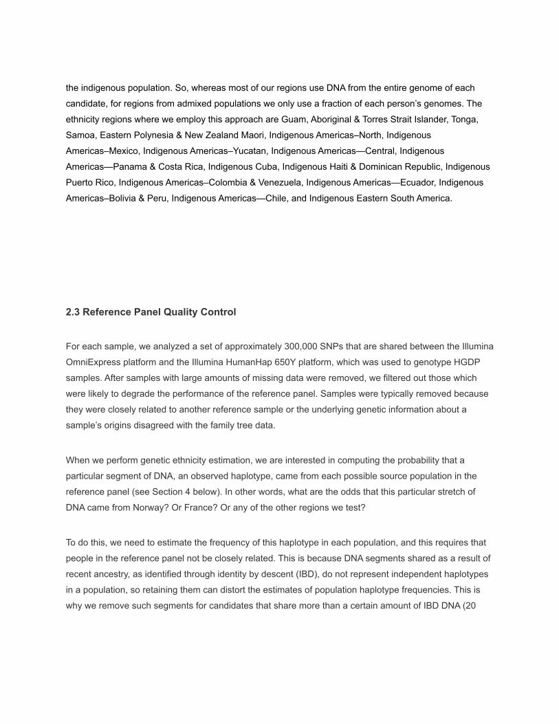
the indigenous population. So, whereas most of our regions use DNA from the entire genome of each

candidate, for regions from admixed populations we only use a fraction of each person’s genomes. The

ethnicity regions where we employ this approach are Guam, Aboriginal & Torres Strait Islander, Tonga,

Samoa, Eastern Polynesia & New Zealand Maori, Indigenous Americas–North, Indigenous

Americas–Mexico, Indigenous Americas–Yucatan, Indigenous Americas—Central, Indigenous

Americas—Panama & Costa Rica, Indigenous Cuba, Indigenous Haiti & Dominican Republic, Indigenous

Puerto Rico, Indigenous Americas–Colombia & Venezuela, Indigenous Americas—Ecuador, Indigenous

Americas–Bolivia & Peru, Indigenous Americas—Chile, and Indigenous Eastern South America.

2.3 Reference Panel Quality Control

For each sample, we analyzed a set of approximately 300,000 SNPs that are shared between the Illumina

OmniExpress platform and the Illumina HumanHap 650Y platform, which was used to genotype HGDP

samples. After samples with large amounts of missing data were removed, we filtered out those which

were likely to degrade the performance of the reference panel. Samples were typically removed because

they were closely related to another reference sample or the underlying genetic information about a

sample’s origins disagreed with the family tree data.

When we perform genetic ethnicity estimation, we are interested in computing the probability that a

particular segment of DNA, an observed haplotype, came from each possible source population in the

reference panel (see Section 4 below). In other words, what are the odds that this particular stretch of

DNA came from Norway? Or France? Or any of the other regions we test?

To do this, we need to estimate the frequency of this haplotype in each population, and this requires that

people in the reference panel not be closely related. This is because DNA segments shared as a result of

recent ancestry, as identified through identity by descent (IBD), do not represent independent haplotypes

in a population, so retaining them can distort the estimates of population haplotype frequencies. This is

why we remove such segments for candidates that share more than a certain amount of IBD DNA (20

cM). Details about our approach for detecting shared segments of IBD DNA can be found in our

AncestryDNA Matching white paper.

Next, we remove samples from the reference panel candidate set when the genetic data about ethnicity

disagrees with what that person has reported about their ethnicity–when underlying genetic information

disagrees with the pedigree data. We identify these outliers using two approaches: (1) we identify clear

outliers using our previous ethnicity estimate version, and (2) we use principal component analysis (PCA).

PCA is frequently used for exploratory data analysis in population genetics research (Jackson 2003).

When applied correctly to genotype data, PCA can capture the genetic variation separating distinct

populations (Patterson 2006).

We apply PCA to the samples that have made it through the previous screening processes and plot the

early stages of the analysis, the “first four principal components,” as a series of scatter plots. We color

each sample by their country of origin, determined by pedigree for Ancestry samples and by sample label

for public samples (see Figure 3.3).

Figure 2.2: PCA Analysis on European Panel Candidates. Scatter plot of the first two components from a principal component

analysis (PCA) of candidate European samples for the AncestryDNA reference panel. Visual inspection of PCA is useful for

numerous aspects of data QC. First, it can be used to identify individual outliers, such as the Italian samples (green squares) that

appear near the Portugal and Spain (yellow and blue triangles, respectively) cluster. It can also be useful for identifying poor sample

grouping. Finally, it can reveal regions where there is limited genetic separation and clusters overlap (e.g. the United Kingdom and

Ireland) and regions that can be further subdivided.

Each population tends to form a cluster of points (each point is a sample) in the scatter plot. This is

because points that are more genetically similar are closer in PCA space. Helpfully, these clusters of

points tend to match geography as well because most people are genetically more similar to others from

nearby. Furthermore, these plots quickly reveal outlier samples which are not near other samples from the

same population. For example, the green circles near purple squares and pink circles indicate samples

with family trees from Italy, but their DNA is more similar to people from Spain and Portugal. These are

examples where the specified population of origin disagrees with the genetic origin represented in PCA

space.

We visually inspect candidates for removal based on a scatterplot like the one in Figure 2.2. Because

different collections of samples reveal different amounts of population structure, PCA and outlier removal

are repeated for different subsets of data. We first remove outliers at the global level (all samples

together), then at the continental level (e.g., outliers in a PCA using only European samples), then at the

regional level (e.g., outliers in a PCA of all Scandinavian samples), and finally at the population level (e.g.,

outliers from a PCA of Norway).

2.4 Iterative Reference Panel Refinement

After removing PCA outliers, we divide our global reference panel into populations corresponding to

distinct genetic clusters in the PCA plots. Before using the reference set to estimate ethnicities of

AncestryDNA customers, we first determine its quality by measuring the performance of our ethnicity

estimation on the reference set itself. How well does our ethnicity estimation do on samples that by

definition are 100% of a single ethnicity?

To do this, we remove 5% of samples from the reference panel and estimate their ethnicity using the

remaining 95% of samples as the new reference panel. We repeat this process 20 times, each time

removing a different 5% of the panel and estimating their genetic ethnicities using the remaining 95%. We

then look at the average predicted ethnicity for samples from each region in the reference set using the

results of these cross-validation experiments. Figure 2.3 shows the results of this experiment as box

plots.

Figure 2.3: 20-fold cross-validation analysis of the Ethnicity 2021 reference panel. Here we plot the results of an experiment in

which 5% of samples are removed from the reference panel, and their ethnicity is estimated using the remaining (95%) panel

samples. Each boxplot represents the distribution of estimated ethnicity for all samples from a given region (75%, 50%, and 25%

percentiles of estimated ethnicity). For the majority of samples in each region, we predict on average 86.0%of the genetic ethnicity

to be from the correct region. And for the most part, the other 14.0% comes from nearby regions. However, there are exceptions. In

particular, our average prediction accuracy for samples for Indigenous Cuba and Burusho are not quite as high. There are many

factors affecting the accuracy of these numbers, most importantly the number of reference samples in the panel for each region and

the genetic distinctness of each region.

The purpose of this analysis is twofold. First, reference panel samples with extremely poor performance in

the cross-validation analysis are removed, as they may poorly represent their ethnic group of origin.

Second, the cross-validation experiments allow us to demonstrate our ability to accurately estimate the

ethnicities of our reference panel samples using our ethnicity estimation method (see section 3) and thus

help us redefine population boundaries. For example, we may merge two populations if performance in

the cross-validation experiment is poor in each group but is found to be better in a merged group.

After performing several rounds of reference panel refinement based on cross-validation experiments, we

settled on dividing our latest reference panel into 77 global regions. These regions are described in

further detail below.

2.5 Updated Reference Panel

The updated AncestryDNA ethnicity estimation reference panel contains 56,580 samples carefully

selected as described above to represent 77 global regions (Table 2.1), each with a unique genetic

profile. As a comparison, our previous panel of 44,703 samples represented 70 distinct global regions.

Region Number of samples

Aboriginal & Torres Strait Islander 53

Aegean Islands 366

Anatolia & the Caucasus 368

Arabian Peninsula 105

Baltics 245

Basque 98

Bengal 228

Benin & Togo 487

Burusho 23

Cameroon, Congo & Western Bantu Peoples 533

Central Asia–South 573

Cyprus 258

Dai 90

Eastern Bantu Peoples 167

Eastern Europe & Russia 1,454

Eastern Polynesia & New Zealand Maori 244

Egypt 252

England & Northwestern Europe 1,907

Ethiopia & Eritrea 98

European Jewish 447

Finland 401

France 3,099

Germanic Europe 3,261

Greece & Albania 482

Guam 133

Indigenous Americas–Bolivia & Peru 371

Indigenous Americas–Colombia & Venezuela 3,162

Indigenous Americas–Mexico 697

Indigenous Americas–North 2,000

Indigenous Americas–Yucatan 302

Indigenous Americas—Central 1,614

Indigenous Americas—Chile 467

Indigenous Americas—Ecuador 691

Indigenous Americas—Panama & Costa Rica 475

Indigenous Arctic 36

Indigenous Cuba 3,408

Indigenous Eastern South America 2,671

Indigenous Haiti & Dominican Republic 2,840

Indigenous Puerto Rico 4,773

Iran/Persia 774

Ireland 794

Ivory Coast & Ghana 272

Japan 150

Khoisan, Aka & Mbuti Peoples 38

Korea 280

Levant 225

Mali 458

Malta 104

Melanesia 91

Mongolia & Central Asia–North 237

Nigeria 569

Northern India 614

Northern Africa 287

Northern Asia 41

Northern China 340

Northern Italy 1,179

Northern Philippines 210

Norway 790

Portugal 893

Samoa 96

Sardinia 75

Scotland 1,797

Senegal 168

Somalia 41

Southeast Asia 287

Southern India 114

Southern Bantu Peoples 183

Southern China 479

Southern Italy 1,365

Southern Japanese Islands 63

Southern Philippines 272

Spain 917

Sweden & Denmark 1,053

The Balkans 1,325

Tonga 121

Vietnam 235

Wales 764

Total 56,580

Table 2.1: The Final AncestryDNA 2021 Ethnicity Reference Panel

We discuss more detailed tests of the performance of the 2021 ethnicity panel in Section 4. For details of

the method AncestryDNA uses for genetic ethnicity estimation, see Section 3.

3. AncestryDNA Ethnicity Estimation

3.1 Introduction

After establishing and validating the reference panel, the next step is to estimate a customer’s ethnicity bycomparing over 300,000 single nucleotide polymorphisms (SNPs) from their DNA to those of thereference panel. We assume that an individual’s DNA is a mixture of DNA from the 77 populationsrepresented in the reference panel. This is illustrated in Figure 3.1, where, because of recombination, acustomer inherits long stretches of DNA from his or her four grandparents who, in this example, comefrom four “single source” reference populations.

Because DNA is passed down from one generation to the next in long segments, it is likely that the DNAat two nearby loci in the genome were inherited from the same person and so the same population (formore details on DNA inheritance see our DNA Matching White Paperhttp://dna.ancestry.com/resource/whitePaper/AncestryDNA-Matching-White-Paper). This means we canget more accurate results by looking at multiple nearby SNPs together as a group, or haplotype, insteadof looking at each SNP in isolation. Our method takes advantage of this to greatly improve our estimates.

We estimate a customer's genetic ethnicity by assuming that each segment of their genome comes fromone of the 77 populations in the reference panel. We divide the customer’s genome into 1,001 windows.

We assume that each window is small enough that each of the two parental haplotypes present in thewindow came from exactly one population. We then combine information from all the windows to estimatewhat overall portion of the customer’s genome came from each of the populations in the reference panelusing a hidden Markov model (HMM).

As you can see in Figure 3.1, each window does not have to have a single ethnicity associated with it.Instead, it can have one from one parent and one from the other. For example, the first window has twodifferent ethnicities represented by the colors green and red. Any ethnicity estimator that uses thetechnology AncestryDNA does to read DNA has to account for the possibility of two separate ethnicities ineach window. In other words, it has to employ a model that looks at the DNA and can identify the DNA asa mix of red and green as opposed to just red or just green (or any of the other possible combinations).

Figure 3.1: Inheritance of DNA from different populations. On the left, we present a three-generation genetic family tree. For

each individual, we show two vertical bars representing the two copies of a single chromosome present in each individual. These

bars are colored to show the reference population from which they inherited their DNA. Each of the four grandparents (solid bars,

top row) has inherited 100% of their DNA from a single population that is different from the other three. The DNA is passed forward

to the parents and finally to the customer, who, through the process of recombination and assortment, ends up inheriting a shuffled

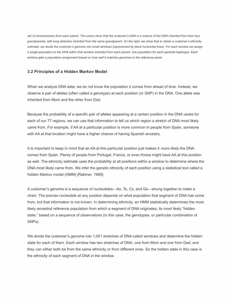
set of chromosomes from each parent. The colors show that the customer’s DNA is a mixture of the DNA inherited from their four

grandparents, with long stretches inherited from the same grandparent. On the right, we show that to obtain a customer’s ethnicity

estimate, we divide the customer’s genome into small windows (represented by black horizontal lines). For each window we assign

a single population to the DNA within that window inherited from each parent, one population for each parental haplotype. Each

window gets a population assignment based on how well it matches genomes in the reference panel.

3.2 Principles of a Hidden Markov Model

When we analyze DNA data, we do not know the population it comes from ahead of time. Instead, we

observe a pair of alleles (often called a genotype) at each position (or SNP) in the DNA. One allele was

inherited from Mom and the other from Dad.

Because the probability of a specific pair of alleles appearing at a certain position in the DNA varies for

each of our 77 regions, we can use that information to tell us which region a stretch of DNA most likely

came from. For example, if AA at a particular position is more common in people from Spain, someone

with AA at that location might have a higher chance of having Spanish ancestry.

It is important to keep in mind that an AA at this particular position just makes it more likely the DNA

comes from Spain. Plenty of people from Portugal, France, or even Korea might have AA at this position

as well. The ethnicity estimate uses the probability at all positions within a window to determine where the

DNA most likely came from. We infer the genetic ethnicity of each position using a statistical tool called a

hidden Markov model (HMM) [Rabiner, 1989].

A customer’s genome is a sequence of nucleotides—As, Ts, Cs, and Gs—strung together to make a

chain. The precise nucleotide at any position depends on what population that segment of DNA has come

from, but that information is not known. In determining ethnicity, an HMM statistically determines the most

likely ancestral reference population from which a segment of DNA originates, its most likely “hidden

state,” based on a sequence of observations (in this case, the genotypes, or particular combination of

SNPs).

We divide the customer’s genome into 1,001 stretches of DNA called windows and determine the hidden

state for each of them. Each window has two stretches of DNA, one from Mom and one from Dad, and

they can either both be from the same ethnicity or from different ones. So the hidden state in this case is

the ethnicity of each segment of DNA in the window.

In addition, with this release we updated our algorithm to be able to tell which ethnicities were inherited

from one parent and which ethnicities were inherited from the other parent. Our phasing algorithm (the

way we assign DNA as coming from each parent, described in AncestryDNA matching white paper) may

make some errors by accidentally assigning one parent’s DNA to the other parent and vice versa. Thus,

we also keep track of whether the HMM thinks we need to swap the DNA our phasing algorithm assigned

to each parent in each window.

HMMs have two components, called emission and transition probabilities. Emission probabilities tell us

how likely it is that a stretch of DNA came from each of the 77 populations based on the observed

sequence. The transition probability indicates how likely it is that there will be a change in the population

identification from one window to the next. In other words, if the DNA in the current window is from only

Norway, how likely is the DNA in the next window to also be from only Norway?

This is a sensible model for human DNA because human genomes are organized linearly along

chromosomes. Additionally, the nature of inheritance means that whole segments of the genome, and,

therefore, many consecutive nucleotides that Ancestry looks at along a chromosome, will have the same

DNA ancestry.

3.3 Inferring Ethnicity Estimates from a Genome-Wide HMM

At AncestryDNA, we use microarrays to obtain DNA data from customer samples. We look at over

700,000 individual locations on the DNA (SNPs) and determine the nucleotides at each position. For

example, we may see an A and a T at position 1, a G and a G at position 2, and so on. We use around

300,000 of these SNPs in the ethnicity estimate.

In working with data from arrays, it is important to remember that people have two copies of each of the

22 chromosomes that AncestryDNA reports data back on. One set of chromosomes comes from Mom

and the other from Dad. This means there are two results for each position AncestryDNA analyzes, and

those results must be interpreted to assign which DNA came from which set of chromosomes (this

process is called phasing). AncestryDNA must consider what possible combinations of ethnicities might

look like. For example, if one customer has a section of their DNA that came from Swedish ancestors

from Mom’s side of the family and Korean ancestors on Dad’s, the algorithm must be able to distinguish

this from a second customer with Swedish and Nigerian ancestors. In addition, because our phasing

algorithm sometimes misassigns which DNA came from one parent and which DNA came from the other

parent, we can use the fact that each parent has different ancestry to improve our assignments of which

DNA came from each, and we include that as part of the hidden state.

We create a genome-wide HMM (illustrated in Figure 3.2) where each possible ethnicity combination (or

hidden state) is represented by which population one parent’s DNA could be from and which population

the other parent’s DNA could be from in a window of the genome, and changes between windows that are

next to each other are unlikely to change the state. In other words, if in the preceding window the DNA

from one parent and the DNA from the other parent both came from Nigeria, then the next window is

more likely to be the same.

The state in a given window is a pair of populations, one assigned to one parent and one assigned to the

other, where each ethnicity in the pair can be different (e.g., red and green in window 1 of the third row of

Figure 3.2) or the same (e.g., green and green in window 1 of the top row of Figure 3.2). Each population

pair assignment has a probability of appearing (or the “observed genotypes”) in the window (emission

probability). In order to fix the errors from our phasing algorithm, we now also keep track whether or not

the model thinks that the DNA assigned to one parent and the other parent needs to be flipped.

We also account for the probability of changing population assignments between adjacent windows

(transition probability). Essentially this means that if you are, for example, Norway/Norway in one window,

there will need to be very strong evidence from the observed DNA data that the neighboring window has

a different population assignment. By applying these probabilities to the whole genome, we can obtain a

sequence of population assignments along a customer's genome.

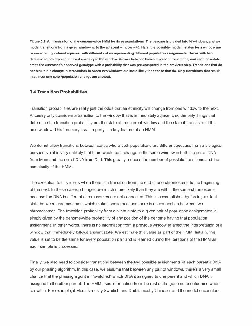
Figure 3.2: An illustration of the genome-wide HMM for three populations. The genome is divided into W windows, and we

model transitions from a given window w, to the adjacent window w+1. Here, the possible (hidden) states for a window are

represented by colored squares, with different colors representing different population assignments. Boxes with two

different colors represent mixed ancestry in the window. Arrows between boxes represent transitions, and each box/state

emits the customer’s observed genotype with a probability that was pre-computed in the previous step. Transitions that do

not result in a change in state/colors between two windows are more likely than those that do. Only transitions that result

in at most one color/population change are allowed.

3.4 Transition Probabilities

Transition probabilities are really just the odds that an ethnicity will change from one window to the next.

Ancestry only considers a transition to the window that is immediately adjacent, so the only things that

determine the transition probability are the state at the current window and the state it transits to at the

next window. This “memoryless” property is a key feature of an HMM.

We do not allow transitions between states where both populations are different because from a biological

perspective, it is very unlikely that there would be a change in the same window in both the set of DNA

from Mom and the set of DNA from Dad. This greatly reduces the number of possible transitions and the

complexity of the HMM.

The exception to this rule is when there is a transition from the end of one chromosome to the beginning

of the next. In these cases, changes are much more likely than they are within the same chromosome

because the DNA in different chromosomes are not connected. This is accomplished by forcing a silent

state between chromosomes, which makes sense because there is no connection between two

chromosomes. The transition probability from a silent state to a given pair of population assignments is

simply given by the genome-wide probability of any position of the genome having that population

assignment. In other words, there is no information from a previous window to affect the interpretation of a

window that immediately follows a silent state. We estimate this value as part of the HMM. Initially, this

value is set to be the same for every population pair and is learned during the iterations of the HMM as

each sample is processed.

Finally, we also need to consider transitions between the two possible assignments of each parent’s DNA

by our phasing algorithm. In this case, we assume that between any pair of windows, there’s a very small

chance that the phasing algorithm “switched” which DNA it assigned to one parent and which DNA it

assigned to the other parent. The HMM uses information from the rest of the genome to determine when

to switch. For example, if Mom is mostly Swedish and Dad is mostly Chinese, and the model encounters

a place where it thinks Mom’s DNA is Chinese and Dad’s DNA is Swedish, it will flip the assignment at

that point.

3.5 Emission Probabilities

Determining how likely the DNA in a window came from a population (the emission probability) is a

complicated process and is described in more detail in our scientific paper Ancestry Inference Using

Reference Labeled Clusters of Haplotypes.

Briefly, our approach includes the following steps:

I. Define the windows. DNA is inherited in long stretches of contiguous DNA within chromosomes

referred to as haplotypes. Working with these blocks of DNA can be more informative than

working with individual positions within the DNA. We do not know the exact haplotype

boundaries, which differ between people, but we can achieve a good approximation by dividing

the genome into 1,001 small windows. Each window covers one section of a single chromosome

and is small enough (e.g., 3-10 centimorgans) that both the maternal and paternal haplotype, the

DNA from Mom and the DNA from Dad, in a given window are likely to each come from a single,

though not necessarily the same, population.

II. Create the haplotype models. Next we need to compare a customer’s haplotype within a

window to those in our reference panel to assess how likely it is to have come from each

population. For example, how likely are both segments of DNA in a haplotype to come from

Norway vs. one from Norway and one from France, and so on through all of the possibilities. To

do this we first need to create a haplotype model. We do this by constructing a BEAGLE

[Browning, 2007] haplotype cluster model for each window using hundreds of thousands of

haplotypes (see Matching white paper for more on this). Since we start with unphased customer

genotype data, data in which maternal and paternal haplotypes are not distinguished, the model

accounts for all possible haplotypes given a set of genotypes, and each state in a haplotype

cluster model represents a cluster of similar haplotypes.

III. Annotate the reference panel. We want to identify the haplotype clusters in our model that are

associated with each population in the reference panel. Because we are confident in the

geographic origin of members of the reference panel, we are able to calculate the probability that

a haplotype from a given population is represented by a particular haplotype cluster. These

values are used to compute the emission probabilities in the genome-wide HMM that assigns

ethnicity.

IV. Compare the test sample to the reference panel to assign population labels using an HMM.To do this, we compute the likelihood that the pair of haplotypes present in each window of a test

sample come from the populations in the reference panel. For each window, both haplotypes may

come from the same population or from different populations, and the resulting emission

probabilities are calculated for all possible combinations.

HMMs are used in a number of existing approaches for estimating ancestral proportions [Maples 2013].

The key part of our method is step III, where we use rich haplotype models in each window, annotated

with population labels from the haplotypes in our reference panel, to assign a likelihood over all

population labels to the haplotypes in our test sample. It is worth noting that our method lends itself to

high-throughput ethnicity estimation, as steps (I) through (III) above–learning the haplotype models from a

large training set and then annotating them with the reference panel populations–need only be carried out

once.

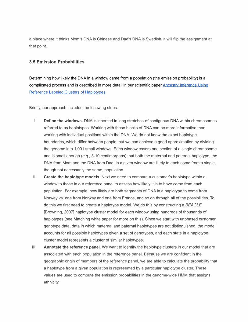
3.6 HMM Model

We use HMMs because they can effectively consider all possible ethnicity assignments to all windows in

the genome and do so efficiently. Ancestry runs our HMM on a customer’s DNA to find the most likely

sequence of ethnicities along the DNA. In more technical terms, the algorithm takes the “Viterbi” path, the

sequence of hidden states that returns the highest probability. The final ethnicity proportions the

customers receive are calculated by counting the proportion of the Viterbi path (weighted by

recombination distance) that are assigned to a particular population in the reference panel. For example,

a customer with the sequence Scotland/Scotland, Scotland/Scotland, Scotland/Scotland,

Ireland/Scotland, Ireland/Scotland (and an incredibly small genome!) would be 20% Ireland and 80%

Scotland, given the five windows have identical size.

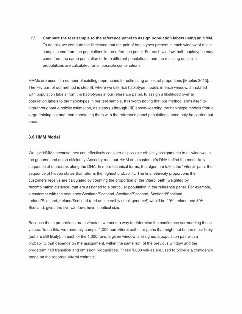
Because these proportions are estimates, we need a way to determine the confidence surrounding these

values. To do this, we randomly sample 1,000 non-Viterbi paths, or paths that might not be the most likely

(but are still likely). In each of the 1,000 runs, a given window is assigned a population pair with a

probability that depends on the assignment, within the same run, of the previous window and the

predetermined transition and emission probabilities. These 1,000 values are used to provide a confidence

range on the reported Viterbi estimate.

Figure 4.6: Illustration of the Viterbi path, represented by arrows, through the HMM that determines an ethnicity estimate.

`

Figure 4.7: Illustration of our stochastic path-sampling process.

4. Assessing Ethnicity Estimation Performance

After developing and optimizing both the estimation process and the reference panel, the finalstep is to determine how well they perform together at assigning ethnicity. Basically, we see howclose our process gets to the right answer through rigorous testing using a wide variety of testcases with known ethnicity.

4.1 Cross-Validation

We evaluate the performance of the ethnicity estimation process by running it on two differenttest cases where we know what the correct answer should be: single-origin individuals(including synthetic single-origin individuals) from the reference panel and synthetic individualswith mixed ethnicities. We gauge its effectiveness by seeing how close we get to the trueethnicity.

Reference panel groups: Our reference panel has two types of reference groups. In the first,people have a long family history in a single region with no influx of other individuals to thatregion. They represent a typical person from that region and by definition, have 100% of theregion they represent in their DNA. The second group is a little more complex. This grouprepresents indigenous peoples who also have ancestors from a different region. An examplewould be people from Mexico who may have Native American, European, and Africanancestors. We are able to include only the parts of their DNA that are Native American (orindigenous) to the reference panel.

Single-origin individuals: We use two different sets of single-origin individuals in our crossvalidation studies. The first are those for whom we utilize their entire genome as a reference fora particular region. By definition these individuals in our reference panel each have 100% of asingle ethnicity.

This approach does not work for the reference panel regions where we used the indigenousDNA of admixed individuals. For these reference panel regions, primarily from the Americas andOceania, we created synthetic single-origin individuals by piecing together genotype sequencesthat represented indigenous ancestry from multiple individuals. These synthetic single-originindividuals are then used to evaluate the accuracy of our method.

We evaluate our process by running 20-fold cross-validation experiments using thesesingle-origin individuals from our reference panel. For example, if we had 100 people in eachreference panel group, we would take 5 from each of the 77 groups and run the algorithm onthese 385 samples using the remaining 7,315 individuals as the reference group. Then adifferent 5 would be taken from each group and the process repeated 20 times so that everyindividual in the reference panel is tested.

Overall we observe that the updated process correctly assigns an average of 84.2% of thegenetic ethnicity to the correct region for single-origin individuals from our reference panel

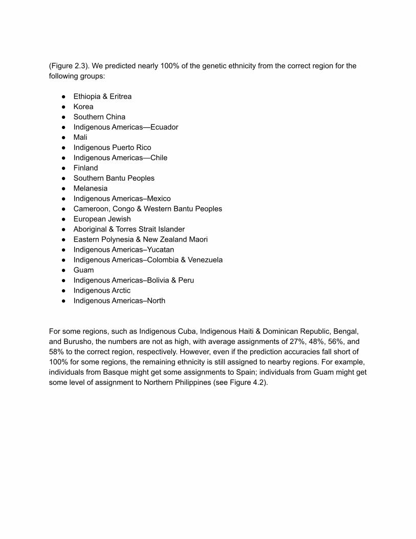
(Figure 2.3). We predicted nearly 100% of the genetic ethnicity from the correct region for thefollowing groups:

● Ethiopia & Eritrea● Korea● Southern China● Indigenous Americas—Ecuador● Mali● Indigenous Puerto Rico● Indigenous Americas—Chile● Finland● Southern Bantu Peoples● Melanesia● Indigenous Americas–Mexico● Cameroon, Congo & Western Bantu Peoples● European Jewish● Aboriginal & Torres Strait Islander● Eastern Polynesia & New Zealand Maori● Indigenous Americas–Yucatan● Indigenous Americas–Colombia & Venezuela● Guam● Indigenous Americas–Bolivia & Peru● Indigenous Arctic● Indigenous Americas–North

For some regions, such as Indigenous Cuba, Indigenous Haiti & Dominican Republic, Bengal,and Burusho, the numbers are not as high, with average assignments of 27%, 48%, 56%, and58% to the correct region, respectively. However, even if the prediction accuracies fall short of100% for some regions, the remaining ethnicity is still assigned to nearby regions. For example,individuals from Basque might get some assignments to Spain; individuals from Guam might getsome level of assignment to Northern Philippines (see Figure 4.2).

Figure 4.2: Average estimated ethnicities for single-origin individuals from each population. In this graph, each rowrepresents single-origin individuals from the population listed. Each column represents each of the possible 77 ethnicitiesthat the single-origin individual might be assigned to. The graph is set up such that the matching individual and his or herethnicity are aligned along the diagonal line. If the algorithm worked perfectly, there would be only red boxes along thediagonal—red represents 100% origin from that population. Any boxes that are not on the diagonal represent misassignedpopulations. This graph also shows that certain ethnicities can be confounded by other ethnicities. For example,individuals with 100% Germanic Europe ethnicity can be assigned to England & Northwestern Europe and Sweden &Denmark.

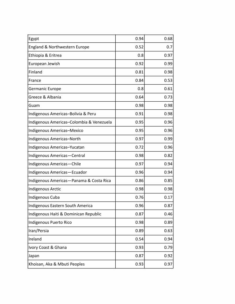
Synthetic individuals with mixed ethnicities: We also evaluated the accuracy of ethnicityestimates for “synthetic” individuals of mixed ethnicity origins. These test cases are simulationswe construct with known mixtures of ethnicities. Each synthetically admixed individual can haveas few as 2 or as many as 27 ethnicity regions, with various proportions. Since the true ethnicityproportions are known, we can calculate precision and recall for each ethnicity region. Precisionand recall are two important factors in evaluating our estimation process.

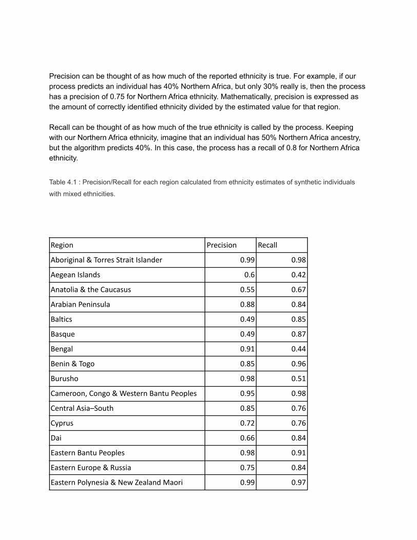
Precision can be thought of as how much of the reported ethnicity is true. For example, if ourprocess predicts an individual has 40% Northern Africa, but only 30% really is, then the processhas a precision of 0.75 for Northern Africa ethnicity. Mathematically, precision is expressed asthe amount of correctly identified ethnicity divided by the estimated value for that region.

Recall can be thought of as how much of the true ethnicity is called by the process. Keepingwith our Northern Africa ethnicity, imagine that an individual has 50% Northern Africa ancestry,but the algorithm predicts 40%. In this case, the process has a recall of 0.8 for Northern Africaethnicity.

Table 4.1 : Precision/Recall for each region calculated from ethnicity estimates of synthetic individuals

with mixed ethnicities.

Region Precision Recall

Aboriginal & Torres Strait Islander 0.99 0.98

Aegean Islands 0.6 0.42

Anatolia & the Caucasus 0.55 0.67

Arabian Peninsula 0.88 0.84

Baltics 0.49 0.85

Basque 0.49 0.87

Bengal 0.91 0.44

Benin & Togo 0.85 0.96

Burusho 0.98 0.51

Cameroon, Congo & Western Bantu Peoples 0.95 0.98

Central Asia–South 0.85 0.76

Cyprus 0.72 0.76

Dai 0.66 0.84

Eastern Bantu Peoples 0.98 0.91

Eastern Europe & Russia 0.75 0.84

Eastern Polynesia & New Zealand Maori 0.99 0.97

Egypt 0.94 0.68

England & Northwestern Europe 0.52 0.7

Ethiopia & Eritrea 0.8 0.97

European Jewish 0.92 0.99

Finland 0.81 0.98

France 0.84 0.53

Germanic Europe 0.8 0.61

Greece & Albania 0.64 0.73

Guam 0.98 0.98

Indigenous Americas–Bolivia & Peru 0.91 0.98

Indigenous Americas–Colombia & Venezuela 0.95 0.96

Indigenous Americas–Mexico 0.95 0.96

Indigenous Americas–North 0.97 0.99

Indigenous Americas–Yucatan 0.72 0.96

Indigenous Americas—Central 0.98 0.82

Indigenous Americas—Chile 0.97 0.94

Indigenous Americas—Ecuador 0.96 0.94

Indigenous Americas—Panama & Costa Rica 0.86 0.85

Indigenous Arctic 0.98 0.98

Indigenous Cuba 0.76 0.17

Indigenous Eastern South America 0.96 0.87

Indigenous Haiti & Dominican Republic 0.87 0.46

Indigenous Puerto Rico 0.98 0.89

Iran/Persia 0.89 0.63

Ireland 0.54 0.94

Ivory Coast & Ghana 0.93 0.79

Japan 0.87 0.92

Khoisan, Aka & Mbuti Peoples 0.93 0.97

Korea 0.82 0.93

Levant 0.64 0.77

Mali 0.94 0.97

Malta 0.94 0.91

Melanesia 0.98 0.99

Mongolia & Central Asia–North 0.98 0.81

Nigeria 0.95 0.92

Northern India 0.72 0.79

Northern Africa 0.94 0.92

Northern Asia 0.7 0.75

Northern China 0.91 0.84

Northern Italy 0.63 0.56

Northern Philippines 0.93 0.91

Norway 0.63 0.89

Portugal 0.91 0.68

Samoa 0.92 0.86

Sardinia 0.8 0.86

Scotland 0.63 0.83

Senegal 0.94 0.95

Somalia 0.92 0.88

Southeast Asia 0.98 0.7

Southern India 0.47 0.75

Southern Bantu Peoples 0.97 0.98

Southern China 0.88 0.92

Southern Italy 0.83 0.61

Southern Japanese Islands 0.88 0.93

Southern Philippines 0.93 0.94

Spain 0.8 0.63

Sweden & Denmark 0.58 0.8

The Balkans 0.83 0.66

Tonga 0.88 0.92

Vietnam 0.79 0.87

Wales 0.68 0.92

We found that most ethnicity regions have precision and recall that are both higher than 0.60,especially several regions that perform extremely well:

● Aboriginal & Torres Strait Islander● Melanesia● Indigenous Arctic● Indigenous Americas–North● Guam● Eastern Polynesia & New Zealand Maori● Southern Bantu Peoples● Cameroon, Congo & Western Bantu Peoples● Indigenous Americas–Colombia & Venezuela● European Jewish● Mali● Indigenous Americas–Mexico● Khoisan, Aka & Mbuti Peoples● Indigenous Americas—Chile● Senegal● Indigenous Americas–Bolivia & Peru● Indigenous Americas—Ecuador

Some regions, such as Indigenous Cuba and Aegean Islands have relatively lower recall, 0.17and 0.43 respectively, while some regions, such as Southern India, Basque, and Baltics haverelatively lower precision, 0.47, 0.49, and 0.49 respectively.

4.2 Region Assessment

We have 77 regions in our reference panel, but there are thousands of ethnicities in the world. We don’t

always have ethnicity information but can use people with deep roots from the same country or part of a

country to assess how our regions perform in different parts of the world and to help our customers

interpret their results. To find these individuals, we use customer-created family trees and look for

customers who have consented to research who have all of their ancestors from the same country.

Ideally, we’d use people with all of their grandparents from the same country, but due to low numbers for

some countries we sometimes use parents.

Customers who are not in the reference panel and have deep trees tracing back to a single country are

expected to have high assignments to the regions associated with that country, and this is what we

generally find. For example, Figure 4.3A shows the average ethnicity assignments for 200 customers with

all four grandparents born in Germany and Figure 4.3B shows a similar situation for 200 customers with

all four grandparents born in Korea. As you can see, while most of their assignment is to the Germanic

Europe region, other regions do appear in small but significant amounts. These analyses help ensure that

ethnicity estimates for people from a region agree with expectations.

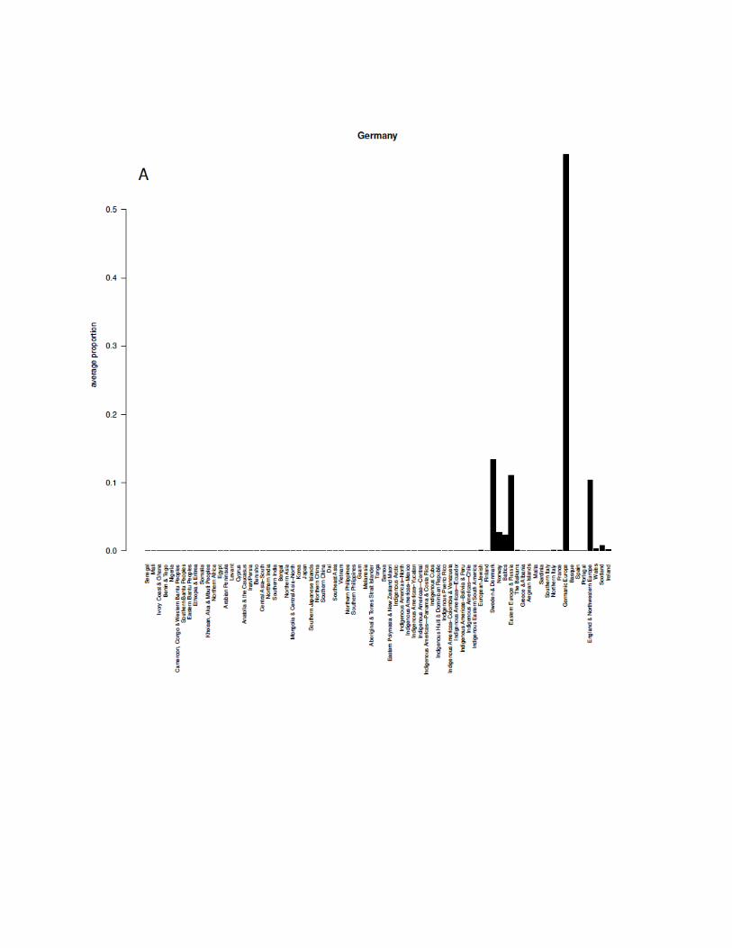
Figure 4.3 Average ethnicity assignments based on grandparental birth location. Average ethnicity assignments for customers

with all four grandparents born in the same country. (A) Germany, (B) South Korea

We also use the maps like the one shown in Figure 4.4 to ensure that ethnicity estimates make sense

geographically. The geographic distribution and amount of ethnicity estimates within a country can often

help make sense of otherwise surprising results. For example, as you can see in Figure 4.4, there is

assignment to the Scotland region in the Brittany region of France. This makes sense because of shared

Celtic ancestry in both Scotland and Brittany, where the Celtic language Breton is traditionally spoken.

Scotland estimates in England also likely reflect its history of Celtic ancestry in that area.

Figure 4.4 Map of average Scotland estimates. Average estimates between 5% and 25% (darker blue) in Wales, England, and

Ireland and between 25% and 50% (light blue) in Brittany likely reflect shared Celtic ancestry.

These analyses help us understand the genetic diversity of the regions and allow us to better

communicate these results to our customers (e.g., even if all of a customer’s ancestors are German, the

customer can expect to have some amount of genetic ethnicity from adjacent regions). These analyses

also aid us in prioritizing future developments for further ethnicity estimation updates.

4.3 Regional Polygon Construction

We divide the world into 77 regions in our reference panel. Each region represents a population with a

unique genetic profile reflecting their shared ancestry. Where possible, we use the known geographic

locations of our samples to guide how we create the regions. Figure 4.5 shows an example of the

information used to define region polygons.

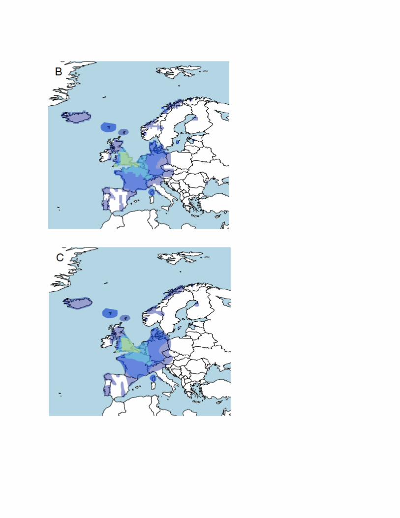
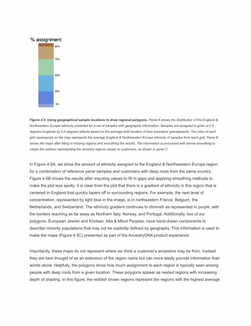
Figure 4.5: Using geographical sample locations to draw regional polygons. Panel A shows the distribution of the England &

Northwestern Europe ethnicity predicted for a set of samples with geographic information. Samples are assigned to grids of 0.5

degrees longitude by 0.5 degrees latitude based on the average birth location of their ancestors’ grandparents. The color of each

grid squarepoint on the map represents the average England & Northwestern Europe ethnicity of samples from each grid. Panel B

shows the maps after filling in missing regions and smoothing the results. The information is processed with kernel smoothing to

create the outlines representing the ancestry regions shown to customers, as shown in panel C.

In Figure 4.5A, we show the amount of ethnicity assigned to the England & Northwestern Europe region

for a combination of reference panel samples and customers with deep roots from the same country.

Figure 4.5B shows the results after imputing values to fill in gaps and applying smoothing methods to

make the plot less spotty. It is clear from the plot that there is a gradient of ethnicity in this region that is

centered in England that quickly tapers off in surrounding regions. For example, the next level of

concentration, represented by light blue in the image, is in northeastern France, Belgium, the

Netherlands, and Switzerland. The ethnicity gradient continues to diminish as represented in purple, with

the borders reaching as far away as Northern Italy, Norway, and Portugal. Additionally, two of our

polygons, European Jewish and Khoisan, Aka & Mbuti Peoples, have hand-drawn components to

describe minority populations that may not be explicitly defined by geography. This information is used to

make the maps (Figure 4.5C) presented as part of the AncestryDNA product experience.

Importantly, these maps do not represent where we think a customer’s ancestors may be from. Instead

they are best thought of as an extension of the region name but can more easily provide information than

words alone. Helpfully, the polygons show how much assignment to each region is typically seen among

people with deep roots from a given location. These polygons appear as nested regions with increasing

depth of shading. In this figure, the reddish brown regions represent the regions with the highest average

assignments. The blue/purple regions have lower average levels. Each set of polygons is accompanied

by a detailed account of the history of the region.

The map below shows polygons for all 77 ethnic groups mostly based on the polygons with 50% or more

assignment, constructed as described above.

4.4 Reporting uncertainty of estimated values

Ethnicity estimates are not an exact science. The percentage AncestryDNA reports to a customer is the

most likely percentage within a range of percentages. In this section, we discuss how we calculate this

range. It is important to keep in mind that here at AncestryDNA we continue to build upon our previous

work to offer ever more accurate results to our customers.

So, for example, we might report someone as 40% England & Northwestern Europe with a confidence

range of 30-60%. This means that they are most likely 40% England & Northwestern Europe but they

could be anywhere between 30% and 60% England & Northwestern Europe.

As discussed in section 3, we run a genome-wide Viterbi estimate on a customer’s DNA sample and

report that back as the customer’s most likely ethnicity estimate. From this we are able to get transition

probabilities that we can then use to generate new ethnicity estimates that while likely, are not the most

likely. The range is based on 1,000 of these sampled paths. For example, if a window has an 80% chance

of being from England & Northwestern Europe, then it has a 20% chance of being from some other

region. The confidence interval captures these sorts of lower chances across a customer’s DNA.

We devised a way, using the 1,000 sampled estimates, to estimate the confidence interval surrounding

the Viterbi estimate reported to the customer. Our objective when defining this approach was to maximize

the probability that the reported range contains the true ancestry proportion (recall), while also

maximizing precision by maintaining a fairly narrow range.

We take the mean and standard deviation of the 1,000 sampled estimates and use these to calculate a

confidence range surrounding the Viterbi estimate. When calculating this range, we take into account the

value of the Viterbi estimate and the population for which we are calculating the range.

We can test our process for calculating the range using synthetic admixed individuals like those used for

the cross-validation studies to determine how often it correctly gets the known ethnicity percentage within

the range. In other words, how often does the range overlap the known ethnicity. We find that the

algorithm performs very well for some populations and less well for others. Since we know the true

ethnicity, we can incorporate correction factors specific for each population to maximize the probability

that the true ethnicity falls within the range.

A large range often reflects the challenges we face because nearby regions have similar DNA. What this

means is that if a customer’s ethnicity estimate has many nearby regions, their ranges will most likely be

larger than if it contained more distant regions. For example, while we may be fairly certain that a

customer has 50% Korea and 50% Portugal ancestry (and therefore small ranges), we may be less sure

about a customer who gets 50% Spain and 50% Portugal. It is relatively easy to tell Korea from Portugal

but relatively hard to tell Portugal from Spain. This may be reflected in the larger ranges for the second

customer. But it is important to keep in mind that we are very confident of the European heritage of

customer two, we are just less certain about how much ancestry is derived from Portugal and how much

from Spain. It is worth noting that, in general, as we increase the precision of our regions (e.g., breaking

Ireland & Scotland into two separate regions), the ranges may become larger, and that this is due to the

fact that DNA from neighboring regions is still very similar.

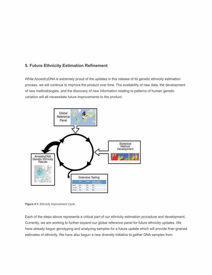
5. Future Ethnicity Estimation Refinement

While AncestryDNA is extremely proud of the updates in this release of its genetic ethnicity estimation

process, we will continue to improve the product over time. The availability of new data, the development

of new methodologies, and the discovery of new information relating to patterns of human genetic

variation will all necessitate future improvements to the product.

Figure 5.1: Ethnicity Improvement Cycle.

Each of the steps above represents a critical part of our ethnicity estimation procedure and development.

Currently, we are working to further expand our global reference panel for future ethnicity updates. We

have already begun genotyping and analyzing samples for a future update which will provide finer-grained

estimates of ethnicity. We have also begun a new diversity initiative to gather DNA samples from

underrepresented regions around the world in order to expand the number of regions we can report back

to customers.

Simultaneously, we are also working to improve our algorithms for ethnicity estimation. Future ethnicity

updates will include an improvement to our statistical methodology that will more fully leverage

information in genetic data to reveal even more information about population history. Along the way, we

always perform thorough testing, involving analyses like those described above. These tests inform the

focus of our improvements and help to refine our improvements as necessary.

Each new release of genetic ethnicity estimation will represent a step forward in our ability to give our

customers a complete description of their genetic ancestry and inform them about their ancient genetic

origins. We hope that, like the entire team at AncestryDNA, our customers will look forward to these future

developments.

6. References

● AncestryDNA DNA matching white paper.https://www.ancestry.com/corporate/sites/default/files/AncestryDNA-Matching-White-Paper.pdf

● Cann HM, de Toma C, Cazes L, Legrand MF, Morel V, Piouffre L, Bodmer J, Bodmer WF,Bonne-Tamir B, Cambon-Thomsen A, Chen Z, Chu J, Carcassi C, Contu L, Du R, Excoffier L,Ferrara GB, Friedlaender JS, Groot H, Gurwitz D, Jenkins T, Herrera RJ, Huang X, Kidd J,Kidd KK, Langaney A, Lin AA, Mehdi SQ, Parham P, Piazza A, Pistillo MP, Qian Y, Shu Q, XuJ, Zhu S, Weber JL, Greely HT, Feldman MW, Thomas G, Dausset J, Cavalli-Sforza LL. Ahuman genome diversity cell line panel. Science, 2002 Apr 12;296(5566):261-2.

● Cavalli-Sforza LL. The Human Genome Diversity Project: past, present and future. Nat RevGenet. 2005 Apr;6(4):333-40.

● D.H. Alexander, J. Novembre, and K. Lange. Fast model-based estimation of ancestry inunrelated individuals. Genome Research, 2009. 19:1655–1664.

● International HapMap Consortium. A haplotype map of the human genome. Nature. 2005 Oct437(7063): 1299–1320.

● International HapMap Consortium, K. A. Frazer, D. G. Ballinger, D. R. Cox, D. A. Hinds, L. L.Stuve, R. A. Gibbs, J. W. Belmont, A. Boudreau, P. Hardenbol, S. M. Leal, S. Pasternak, D. A.Wheeler, T. D. Willis, F. Yu, H. Yang, C. Zeng, Y. Gao, H. Hu, W. Hu, C. Li, W. Lin, S. Liu, H.Pan, X. Tang, J. Wang, W. Wang, J. Yu, B. Zhang, Q. Zhang, H. Zhao, et al. A secondgeneration human haplotype map of over 3.1 million SNPs. Nature, 2007 Oct449(7164):851–61.

● Jackson, J.E. A User’s Guide to Principal Components (John Wiley & Sons, New York, 2003).● K. Noto, Y. Wang, M. Barber, J. Granka, J. Byrnes, R. Curtis, N. Myres, C. Ball, and K.

Chahine. Underdog: A fully-supervised phasing algorithm that learns from hundreds of

thousands of samples and phases in minutes., 2014. Invited Talk at the American Society ofHuman Genetics (ASHG) annual meeting, San Diego, CA, October 2014.

● K. Noto, Y. Wang, M Barber, J. Byrnes, P. Carbonetto, R. Curtis, J. Granka, E. Han, A.Kermany, N. Myres, C. Ball, and K. Chahine. Polly: A novel approach for estimating local andglobal admixture proportion based on rich haplotype models. 2015. Invited Talk at theAmerican Society of Human Genetics (ASHG) annual meeting, Baltimore, MD, October 2015.

● Lazaridis, I et. al. Ancient human genomes suggest three ancestral populations forpresent-day Europeans. Nature, 513:409–413, 2014.

● Maples, Brian K., et al. "RFMix: a discriminative modeling approach for rapid and robustlocal-ancestry inference." The American Journal of Human Genetics 93.2 (2013): 278-288.

● Patterson N, Price AL, Reich D. Population Structure and Eigenanalysis. PLoS Genet 20062(12): e190.

● Pritchard JK, Stephens M, Donnelly P. Inference of population structure using multilocusgenotype data. Genetics. 2000 Jun;155(2):945-59.

● Purcell, S. PLINK v1.07. http://pngu.mgh.harvard.edu/purcell/plink/● Purcell S, Neale B, Todd-Brown K, Thomas L, Ferreira MA, Bender D, Maller J, Sklar P, de

Bakker PI, Daly MJ, Sham PC. PLINK: a tool set for whole-genome association andpopulation-based linkage analyses. Am J Hum Genet. 2007 Sep;81(3):559-75.

● Rabiner L. A tutorial on hidden Markov models and selected applications in speechrecognition.Proceedings of the IEEE, 77(2):257–286, 1989.

● S. R. Browning and B. L. Browning. Rapid and accurate haplotype phasing and missing-datainference for whole-genome association studies by use of localized haplotype clustering.American Journal of Human Genetics, 81:1084–1096, 2007.