
E. LPV System and Gain Scheduling E.1 Linear Parameter ... · PDF fileE.1 Linear Parameter...
33
E.1 Linear Parameter Varying(LPV) System E.3 Gain Scheduling E. LPV System and Gain Scheduling E.4 Design Example Reference: [DP05] G.E. Dullerud and F. Paganini, A Course in Robust Control Theory: A Convex Approach, Text in Applied Mathematics, Springer, 2005. [DP05, Sec. 11] E.2 Quadratic Stabilization Robust and Optimal Control, Spring 2015 Instructor: Prof. Masayuki Fujita (S5-303B)
Transcript of E. LPV System and Gain Scheduling E.1 Linear Parameter ... · PDF fileE.1 Linear Parameter...

E.1 Linear Parameter Varying(LPV) System
E.3 Gain Scheduling
E. LPV System and Gain Scheduling
E.4 Design Example
Reference:[DP05] G.E. Dullerud and F. Paganini,
A Course in Robust Control Theory: A Convex Approach,Text in Applied Mathematics, Springer, 2005.
[DP05, Sec. 11]
E.2 Quadratic Stabilization
Robust and Optimal Control, Spring 2015Instructor: Prof. Masayuki Fujita (S5-303B)

2
J. Shamma
A. Packard
LPV Systems and Gain ScheduleJ. Shamma and M. Athans, “Gain scheduling: Potential hazards and possible remedies,”IEEE Control Systems Magazine, 12-3, pp. 101-107, 1992
M. Athans
A. Packard, “Gain-scheduling via linear fractional transformations,” Systems and Control Letters, 22, pp. 79-92, 1994
3
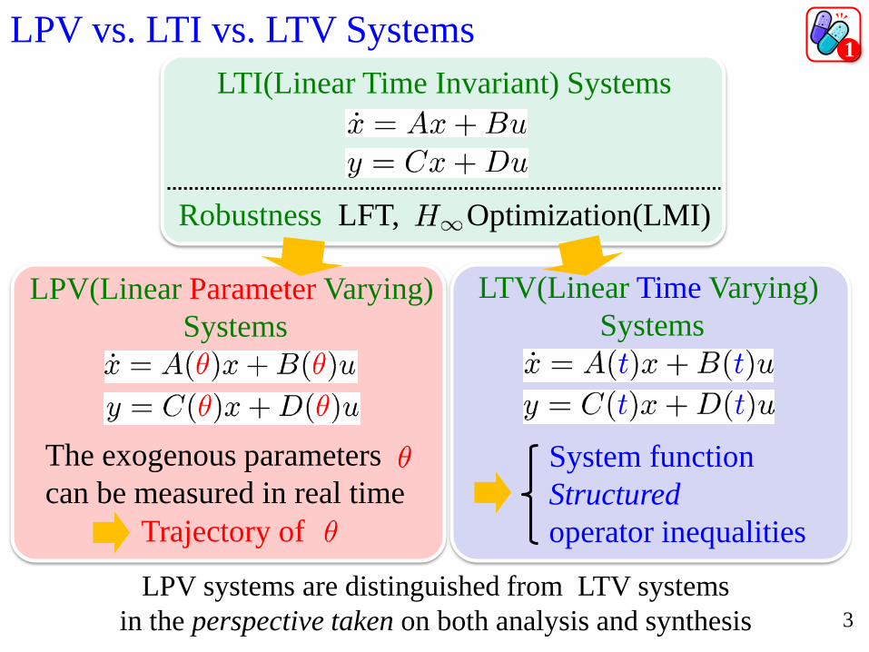
LPV vs. LTI vs. LTV SystemsLTI(Linear Time Invariant) Systems
LTV(Linear Time Varying) Systems
LPV(Linear Parameter Varying) Systems
LPV systems are distinguished from LTV systems in the perspective taken on both analysis and synthesis
Optimization(LMI)LFT,
The exogenous parameters can be measured in real time
Trajectory of
Robustness
System functionStructuredoperator inequalities
1

4
LPV System RepresentationStyle 1: Polytope Representation
: non-singular matrix
Mass-Spring-Damper System[Ex.]
,
, ,
,
psys
pols = psys([M1, … ,Mn])
(Descriptor Representation)
(Convexity)

5
Style 2: Affine parameter-dependent Representation
: real parameters: affine function
LPV System Representation psys
Mass-Spring-Damper System[Ex.]
affs = psys(pv,[s0,s1, … ,sn])
,
pols = aff2pol( affs )

6
LPV System via Jacobian LinearizationNonlinear Plant
: Parametric-dependent exogenous inputEquilibrium Family
: trim point
Scheduling variableLinearization
[Ex.] ,
: equilibrium point

7
LPV System via Jacobian Linearization[Ex.] Longitudinal dynamics of a missileNonlinear Plant
Output : normalized acceleration
: angle of attack,: pitch rate, : tail-fin deflection
Aerodynamic coefficients: Mach number
Equilibrium Family (parametrized by and )
, ,
Linearization
2

8
Quadratic StabilitySystem ,
or differential inclusion:
Polytope Uncertainty
Norm-bounded Uncertainty
The system is quadratically stable if and s.t.,
s.t.
[Ex.]s.t.s.t.
[Ex.]
s.t.
and
( is globally asymptotically stable, which is a hard condition)
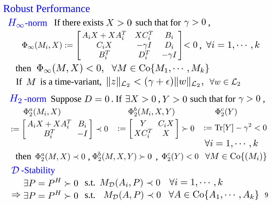
Suppose . If , such that for ,
If there exists such that for ,
9
Robust Performance
then
,
If is a time-variant,
-norm
-norm
-Stabilitythen , ,
s.t.s.t.

10
Quadratic Stabilization with State Feedback
State FeedbackClosed-loop System
Quadratic Stabilization Conditions.t.
and s.t.
Bilinear Matrix Inequality(BMI) (which does not have a feasible method to solve)
BMI to LMI: feasible

11
Polytope-based Gain Scheduling: Representation
LPV Plant
: affine functions of: physical parameters
LPV Controller
,
: measurable

12
where
, : the base of the null space spanned by ,
Minimize such that for
Convex Optimization Problem(LMI)
Polytope-based Gain Scheduling: -like SynthesisObjectives
The closed-loop system is stable for all admissible trajectoriesFind satisfying
3

13
LFT-based Gain Scheduling: Representation
,
: measurable
Closed Loop System
LPV Plant
LPV Controller
,
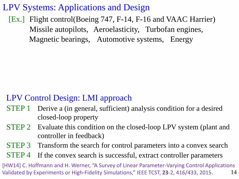
14[HW14] C. Hoffmann and H. Werner, “A Survey of Linear Parameter-Varying Control Applications Validated by Experiments or High-Fidelity Simulations,” IEEE TCST, 23-2, 416/433, 2015.
LPV Systems: Applications and DesignFlight control(Boeing 747, F-14, F-16 and VAAC Harrier)Missile autopilots, Aeroelasticity, Turbofan engines,Magnetic bearings, Automotive systems, Energy
[Ex.]
Derive a (in general, sufficient) analysis condition for a desired closed-loop property
STEP 1
Evaluate this condition on the closed-loop LPV system (plant and controller in feedback)
STEP 2
Transform the search for control parameters into a convex searchSTEP 3If the convex search is successful, extract controller parametersSTEP 4
LPV Control Design: LMI approach

15
Output argument
MATLAB Command
Input argument
hinfgs
[gopt, pdK, R, S] = hinfgs( pdP, r, gmin, tol, tolred )
option
R
gmin lower limit of gopttol , tolred required relative accuracy on gopt and threshold
S, symmetric matrices satisfying Riccati inequalities
pdKgopt
Polytopic Gain Scheduled controllerFeasible optimal closed-loop quadratic performance gain
pdPr
Parameter-dependent plantnumber of control inputs and outputs

16
Missile Model: Model Representation misldemObjective The missile dynamics are strongly dependent on
angle of attack , air speed and altitudeTheir parameters completely define the flight conditions(operating point) of the missile and they are assumed to be measured in real time.
Assumption The pitch, yaw and roll axes are decoupled.Linearized Dynamics of Pitch Channel
: angle of attack, : normalized vertical acceleration: pitch rate, : fin deflection of vertical stabilizer
Aerodynamical coefficients(depending on , and ): available (measurable) in real time
Gulf War(Patriot Missile)
Note: The command misldem does not exist in the newest version.
4

0
106
0.5 4 17
Missile Model: Parameter RepresentationAerodynamical coefficients
Oncoming Flow
Define 100 pairs of Specific Parameters for Verification/Analysis
pNum = 100 ; polyc = [ ] ;% Fixed polytopic coordinatespoly1 = [ 1, 0, 0, 0 ] ; poly2= [ 0, 1, 0, 0 ] ;poly3 = [ 0, 0, 1, 0.] ; poly4 = [ 0, 0, 0, 1 ] ;polyc = [ polyc; poly1; poly2; poly3; poly4 ] ;for j = 1 : 9
poly1 = [ 1-j*0.1, j*0.1, 0, 0 ] ; poly2= [ 0, 1-j*0.1, j*0.1, 0 ] ;poly3 = [ 0, 0, 1-j*0.1, j*0.1 ] ; poly4 = [ j*0.1, 0, 0, 1-j*0.1 ] ;poly5 = [ 1-j*0.1, 0, j*0.1, 0 ] ; poly6 = [ 0, 1-j*0.1, 0, j*0.1 ] ;polyc = [ polyc; poly1; poly2; poly3; poly4; poly5; poly6 ] ;
end% random polytopic coordinatesfor j = 1 : pNum-58
poly= rand(1,4) ; poly= poly/sum(poly) ; polyc = [ polyc; poly ] ;
end
MATLAB Command
,
%Specify the range of parameter valuesZmin=.5; Zmax=4; Mmin=0; Mmax=106; pv=pvec('box',[Zmin Zmax; Mmin Mmax]);
MATLAB Command
pvec

18
,
Missile Model: LPV System via Polytopic Approach
psinfo(pdP) % data of polytopic systempvinfo(pv) % data of parameters
MATLAB Command
Plant
%Specify parameter-dependent models0=ltisys([0 1;0 0],[0;1],[-1 0;0 1],[0;0]);s1=ltisys([-1 0;0 0],[0;0],zeros(2),[0;0],0);s2=ltisys([0 0;-1 0],[0;0],zeros(2),[0;0],0); pdPa=psys(pv,[s0 s1 s2]);pdP = aff2pol( pdPa ) ;
MATLAB Command
figureomega = logspace( -2, 2, 200 ) ;for j = 1 : pNum
Pdp = psinfo(pdP,'eval',polyc(j,:)) ;[adp,bdp,cdp,ddp] = ltiss(Pdp) ;sys = ss(adp,bdp,cdp,ddp) ;[vs] = sigma( sys, omega ) ;semilogx( omega, mag2db( vs ) ) ;hold on ; grid on ;
end
MATLAB Command
psys
ltisys, ltiss, pvinfo

19
Goal
Mixed Sensitivity Problem
Generalized Plant
Missile Model: Problem Specification
Specifications(Performance/Robustness)To control the vertical acceleration over this operation range
The stringent performance specifications
The bandwidth limitation imposed by unmodeled dynamicsfor the step response of the vertical acceleration Settling Time < 0.5 s
missileautopilot

20
Missile Model: Shaping Filters(Weight Functions)
np=2.0101; dp=[1.0000e+00 2.0101e-01];Wp=ltisys('tf',np,dp);nu=[9.6785e+00 2.9035e-02 0 0];du=[1.0000e+00 1.2064e+04 1.1360e+07 1.0661e+10];Wu=ltisys('tf',nu,du);
MATLAB CommandPerformance/Sensitivity Weight
Robustness/Input Weight
2 rad/s 1000 rad/s

21
Missile Model: Generalized Plant
missile
(Gaug)
(‘G’)
(‘r’) (‘K:e’)
(‘G:K’)
inputs = 'r' ;outputs = ‘wp;wu' ;Kin = 'K:e=r-G(1);G(2)' ;[Gaug,r]=sconnect(inputs,outputs,Kin,'G:K',...pdP,‘wp:e',Wp,‘wu:K',Wu);
MATLAB Command
figureomega = logspace( -2, 2, 200 ) ;for j = 1 : pNum
Pdg = psinfo(Gaug,'eval',polyc(j,:)) ;[adg,bdg,cdg,ddg] = ltiss(Pdg) ;sys = ss(adg,bdg,cdg,ddg) ;[vs] = sigma( sys, omega ) ;semilogx( omega, mag2db( vs ) ) ;hold on ; grid on ;
end
MATLAB Command
sconnect

22
Missile Model: Gain Scheduled Controller
(automatic calculation)
OK
% Minimization of gamma for the loop-shaping criterion[gopt,pdK]=hinfgs(Gaug,r,0,1e-2);gopt
MATLAB Command
hinfgs
MATLAB Command WindowSolver for linear objective minimization under LMI constraints
Iterations : Best objective value so far 11112 8035.93758913 5439.90165343 0.245759
*** new lower bound: 0.22753044 0.23669745 0.23514446 0.234688
*** new lower bound: 0.23183447 0.233905
*** new lower bound: 0.231683
Result: feasible solution of required accuracybest objective value: 0.233905guaranteed absolute accuracy: 2.22e-003f-radius saturation: 2.666% of R = 1.00e+008
Optimal quadratic RMS performance: 2.0544e-001
% Form the closed-loop systempCL=slft(Gaug,pdK);
MATLAB Command

23
figureomega = logspace( -4, 4, 300 ) ;for j = 1 : pNum
Pd = psinfo(pdK,'eval',polyc(j,:)) ;[adk,bdk,cdk,ddk] = ltiss(Pd) ;sys = ss(adk,bdk,cdk,ddk) ;[vs] = sigma( sys, omega ) ;semilogx( omega, mag2db( vs ) ) ;hold on ; grid on ;
end
MATLAB Command
Missile Model: LPV Controller
Controller
Elements of Controller

24
Missile Model: Frequency Response AnalysisLoop Transfer Function Closed-loop TF
pdPo = psinfo(pdP,'eval',polyc(j,:)) ;pdKo = psinfo(pdK,'eval',polyc(j,:)) ;Pd = smult(pdKo, pdPo ) ;
MATLAB Command
Pd = psinfo(pCL,'eval',polyc(j,:)) ;MATLAB Command

25
Missile Model: SensitivitySensitivity Complementary Sensitivity
pdPo = psinfo(pdP,'eval',polyc(j,:)) ;pdKo = psinfo(pdK,'eval',polyc(j,:)) ;Pd = smult(pdKo, pdPo ) ;pdS = sloop( eye(2), Pd ) ;
MATLAB CommandpdPo = psinfo(pdP,'eval',polyc(j,:)) ;pdKo = psinfo(pdK,'eval',polyc(j,:)) ;Pd = smult(pdKo, pdPo ) ;pdT = sloop( Pd, eye(2) ) ;
MATLAB Command

Vertical acceleration Control Input
Missile Model: Step Response for vertical acceleration
AZV=[]; U=[]; t=[0:.01:1]';for j=1:pNum
Pcl=psinfo(pCL0,'eval',polyc(j,:));[acl,bcl,ccl,dcl]=ltiss(Pcl);y=step(acl,bcl,ccl,dcl,1,t);AZV=[AZV,1-y(:,1)]; U=[U,y(:,2)/20];
endfigure; grid on; hold on; plot(t,AZV);figure; grid on; hold on; plot(t,U);
MATLAB Command
26
[pdG0,r]=sconnect('r','e=r-G(1);K','K:e;G(2)','G:K',pdP);pCL0=slft(pdG0,pdK);
MATLAB Command
splot

27
Missile Model: Assessment of LPV ControllerTransition on parameters
Vertical acceleration Control Input
pdsimul
Note: The command spiralt does not exist in the newest version.
spiralt
t0=[0:.001:.5];pt=spiralt(t0);figure; plot(pt(1,:),pt(2,:));
MATLAB Command[t,x,y]=pdsimul(pCL0,'spiralt',.5);figure; plot(t,1-y(:,1));figure; plot(t,y(:,2)/20);
MATLAB Command
28
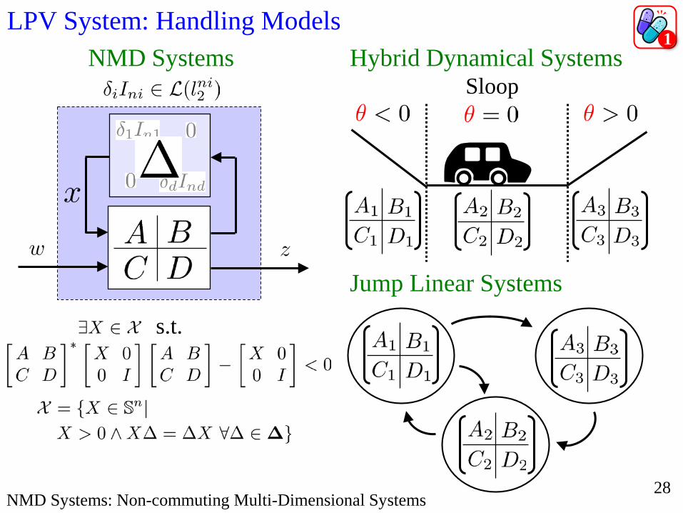
NMD Systems Hybrid Dynamical Systems
Jump Linear Systems
LPV System: Handling Models
NMD Systems: Non-commuting Multi-Dimensional Systems
Sloop
s.t.
1

29
LPV System via quasi-LPVStates divided into two partitions
Tune-varying Parameters
Quasi-LPV form
[Ex.] Longitudinal dynamics of a missile
2

30
LFT-based Gain Scheduling: Synthesis
Conservative Design
where
Minimize satisfying that there exist pairs of symmetric matrices
Find an internally stabilizing controller s.t.
in and in such that
3

31[AGB95] P. Apkarian, P. Gahinet and G. Becker, “Self-Scheduled Control of Linear Parameter-Varying Systems,” Automatica, Vol. 31, No. 9, pp. 1251-1261, 1995.
2DOF controller
Missile Model: Advanced Model and Controller
ActuatorFlexibility
GyroLPV system(pitch channel)
Frequency Response
4

32
P-system and connection commands
−
G3 = sadd(G1,G2) ; G3 = smult(G1,G2) ;
G3 = sdiag(G1,G2) ;
G3 = sloop(G1,G2) ;
[P, r] = sconnect( inputs, outputs, K_in, G1_in, g1, G2_in, g2, … ) ;
G3 = slft(G1,G2, udim, ydim) ;
r=[r(1),r(2)] number of control inputs ( ) and outputs ( ) respectively
P standard plant
ns number of statesni number of inputsno number of outputs
G = ltisys(A,B,C,D,E) ;G = ltisys(‘tf’,num,den) ; %SISO only[A,B,C,D,E] = ltiss(G) ;[num,den] = ltitf(G) ;[ns,ni,no] = sinfo(G) ;
5

33
Data StructureAffine-parameter Representation
LFT Representation
Interconnection
sys = ltisys(A,B,C,D,E) ; sys = ss(A,B,C,D) ;
sconnect sysic
P-system SYSTEM matrix
sys =
USS SYSTEM
Polytopic Representation
[Pnom,delta] = aff2lft(pdP) ;
aff2pol
pvec
Parameter box
-1 2
20
50
pv = pvec('box',[-1 2;20 50]);
Verticespv = pvec('pol',[v1,v2,v3,v4])
6
![Identifying Position-Dependent Mechanical Systems: A Modal ... · (LPV) control framework [15]–[18], which formalizes the gain-scheduling method by ensuring stability and performance](https://static.fdocuments.in/doc/165x107/5ee46af2ad6a402d666d8323/identifying-position-dependent-mechanical-systems-a-modal-lpv-control-framework.jpg)


