e+e- Linear Collider

E.Elsen

DESY Summer Student Programme, 2007

1

Plan of Lecture

• Today

• Introduction to Physics at the Terascale

• Accelerators requirements at the highest energy

• Linear Collider – general concepts

• Luminosity

• Tomorrow

• ILC – piece by piece

2

Physics Need for Terascale

• Standard Model is successfully describing essentially all observed features of particle physics

• Yet, it is known to be incomplete

• Electroweak symmetry breaking

• Origin of mass

• Larger symmetries

• …

3

High Energy Colliders

• Heisenberg

• the highest momenta are required to unravel the smallest features of nature

• best achieved with head-on collision of particles

!x!p ! !

4

Choice of Force

Force rel. strength reach [m] Particle

Gravitation 6×10-39 ∞ all

electrom. 1/137 ∞ charged

strong ~1 10-15–10-16 hadrons

weak 10-5 «10-16 hadrons & leptons

5

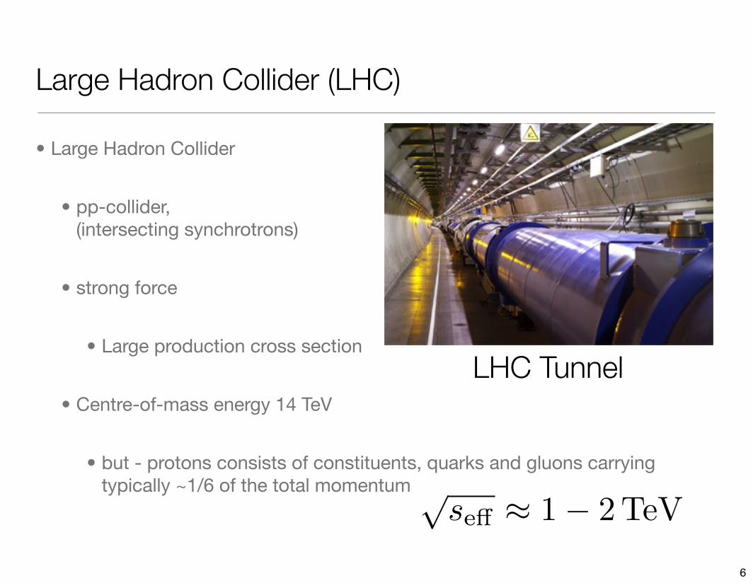
Large Hadron Collider (LHC)

• Large Hadron Collider

• pp-collider,(intersecting synchrotrons)

• strong force

• Large production cross section

• Centre-of-mass energy 14 TeV

• but - protons consists of constituents, quarks and gluons carrying typically ~1/6 of the total momentum

LHC Tunnel

!se! " 1# 2 TeV

6

LHC

• Fast path to highest energies

• economic since protons are heavy and loose little energy due to synchrotron radiation on their circular path

• LHC reuses the tunnel originally built for LEP @ CERN

• will turn on in mid 2008

• first "sighting" of the Terascale

7

Physics Menu of the LHC

• LHC is likely to be a discovery tool for

• Higgs

• Supersymmetric particles or whatever nature chooses to have in store

• extra dimensions

• black holes

• …

Will the LHC be able to discern the options?

much more to come in subsequent

lectures

8

e+e- Linear Collider

• Particle physics has a long history of complementary exploration with hadron and lepton machines, i.e. pp- or ee-colliders

• Features of e+e- colliders:

• point-like particles

• well defined cms energy

• full energy available in cms

• well defined quantum state

• electroweak interaction of beam particles

• requires tremendous luminosity

• many "background processes" vanish as 1/s.!s"

!GeV"

#(e

#e$%

W#W

$(&

))

!p

b" LEP

'e exchange

no ZWW vertex

Standard Model

Data

189 GeV Preliminary

0

10

20

160 170 180 190 200

Example: WW Threshold

9

Higgs Particle Search (Status EPS07)

• mH = 76+33-24 GeVmH < 144 GeV @ 95% CL

• Direct search @ LEPmH > 114 GeV (95% CL)

• Probability MH>114 GeV15%

• so if the Higgs is there and heavier than 114 GeVmH < 182 GeV @ 95% CL

10

Higgs Search @ Hadron Colliders

• a light Higgs particle is difficult to detect at hadron colliders

• several decay modes have to be combined

• sophisticated analyses are required

• Tevatron

• LHC

HIGGS PHYSICS

30 fb!1 for the entire Higgs mass range. Several production and decay channels can be used forthis purpose; see Fig. 2.1-4 (left). The spin–zero nature of the Higgs boson can be determinedand a preliminary probe of its CP nature can be performed. Furthermore, information onthe Higgs couplings to gauge bosons and fermions can be obtained with a higher luminosity;the estimated precision for coupling ratios are typically O(10)% with L = 100 fb!1 [65].Because of the small production rates and large backgrounds, the determination of the Higgsself–coupling is too di!cult and will require a significantly higher luminosity.

)2

(GeV/cH

m

)-1

dis

co

very

lu

min

osit

y (

fb!

5-

1

10

210

100 200 300 500 800

CMSjj"l#WW#qqH, H

""ll#ZZ#qqH, H

, NLO""ll#WW*/WW#H

4 leptons, NLO#ZZ*/ZZ#H

-$+$, %% #qqH, H

inclusive, NLO%%#H

bb#H, WH, HttCombined channels

ATLAS

LEP 2000

ATLAS

mA

(GeV)

tan&

1

2

3

4

5

6

789

10

20

30

40

50

50 100 150 200 250 300 350 400 450 500

0h

0H A

0 +-H

0h

0H A

0 +-H

0h

0H A

00

h H+-

0h H

+-

0h only

0 0Hh

ATLAS - 300 fbmaximal mixing

-1

LEP excluded

FIGURE 2.1-4. The required luminosity that is needed to achieve a 5! discovery signal at LHC usingvarious detection channels as a function of MH [13] (left) and the number of Higgs particles that can bedetected in the MSSM [tan", MA] parameter space [12] (right).

In the MSSM, all the Higgs bosons can be produced for masses below 1 TeV and largeenough tan " values if a large integrated luminosity, ! 300 fb!1, is collected; Fig. 2.1-4 (right).There is, however, a significant region of the parameter space where only the light SM–likeh boson will be found. In such a case the mass of the h boson may be the only characteristicinformation of the MSSM Higgs sector at the LHC. Nevertheless, there are some situationsin which MSSM Higgs searches at the LHC could be slightly more complicated. This is forinstance the case when Higgs decays into SUSY particles such as charginos and (invisible)neutralinos are kinematically accessible and significant. Furthermore, in the so–called intensecoupling regime where the three neutral Higgs particles are very close in mass and have strongcouplings to b–quarks, not all three states can be resolved experimentally [66].

The search of the Higgs particles can be more complicated in some extensions of theMSSM. For instance, if CP–violation occurs, the lighter neutral H1 boson can escape ob-servation in a small region of the parameter space with low MA and tan " values, whilethe heavier H,A and H± bosons can be accessed in smaller areas than in the usual MSSM[42]. In the NMSSM with a relatively light pseudoscalar A1 particle, the dominant decay ofthe lighter CP–even H1 boson could be H1 " A1A1 " 4b, a signature which is extremelydi!cult to detect at the LHC [47]. A possibility that should not be overlooked is that inseveral extensions of the Higgs sector, such as non–minimal SUSY, extra–dimensional modelsand the extension with a singlet scalar field, the Higgs boson might decay invisibly makingits detection at the LHC very challenging if possible at all. In addition, in some other SMextensions, the rates for the dominant gg " H production can be strongly suppressed.

II-16 ILC Reference Design Report

LHC p

rosp

ects

11

HIGGS PHYSICS

2.2.2 Higgs detection at the ILC

In Higgs–strahlung, the recoiling Z boson, which can be tagged through its clean !+!! decays[! = e or µ] but also through decays into quarks which have a much larger statistics, is mono–energetic and the Higgs mass can be derived from the energy of the Z boson since the initiale± beam energies are sharp when beamstrahlung is ignored; the e!ects of beamstrahlung mustthus be suppressed as strongly as possible. Therefore, it will be easy to separate the signalfrom the backgrounds, Fig. 2.2-8 (left). In the low mass range, MH <!140 GeV, the processleads to bb̄qq̄ and bb̄!! final states, with the b quarks being e"ciently tagged by micro–vertexdetectors. For MH >!140 GeV where the decay H " WW " dominates, the Higgs boson canbe reconstructed by looking at the !!+ 4–jet or 6–jet final states, and using the kinematicalconstraints on the fermion invariant masses which peak at MW and MH , the backgroundsare e"ciently suppressed. Also the !!qq̄!" and qq̄qq̄!" channels are easily accessible.

80 100 120 140 160 180 2000

50

100

150

200

250

300

350

400 X-+ -e+e

Missing mass(GeV)

No. of e

ve

nts

/1G

eV

=300GeVs-1

500 fb

µµ

0

0.5

1

1.5

2

2.5

3

3.5

118.5 119 119.5 120 120.5 121 121.5 122

230 GeV

350 GeV

MH GeV

fb/G

eV 230 GeV

350 GeV

FIGURE 2.2-8. Left: distribution of the µ+µ! recoil mass in e+e! " µ+µ!X ; the background fromZ pair production and the SM Higgs signals with various masses are shown [8]. Right: di!erential crosssection for e+e! " HZ " Hµ+µ! for two di!erent c.m. energies with MH = 120 GeV [78].

It has been shown in detailed simulations [7, 79] that only a few fb!1 data are needed toobtain a 5# signal for a Higgs boson with a mass MH <! 150 GeV at a 500 GeV collider, evenif it decays invisibly (as it could happen e.g. in the MSSM). In fact, for such small masses,it is better to move to lower energies where the Higgs–strahlung cross section is larger andthe reconstruction of the Z boson is better [78]; for MH ! 120 GeV, the optimum energy is#

s = 230 GeV as shown in Fig. 2.2-8 (right). Moving to higher energies, Higgs bosons withmasses up to MH ! 400 GeV can be discovered in the Higgs–strahlung process at an energyof 500 GeV and with a luminosity of 500 fb!1. For even larger masses, one needs to increasethe c.m. energy of the collider and, as a rule of thumb, Higgs masses up to ! 80%

#s can

be probed. This means that a 1 TeV collider can probe the entire Higgs mass range that istheoretically allowed in the SM, MH <! 700 GeV.

The WW fusion mechanism o!ers a complementary production channel. For low MH

where the decay H " bb̄ is dominant, flavor tagging plays an important role to suppress the

II-20 ILC Reference Design Report

e+e! ! ZH ! H!"#$ µ+µ!

Higgs Detection Prospects at the ILC

• a light Higgs is easily detected at the ILC

• its properties can be measured

The Higgs in the Standard Model

! !-

-+

+

(GeV)

10

10

1

-3

-2

10-1

SM

Hig

gs

Bran

ch

ing R

ati

o

bb

ggcc

""

MH

W W

100 110 120 130 140 150 160

FIGURE 2.2-12. The branching ratio for the SM Higgs boson with the expected sensitivity at ILC. Aluminosity of 500 fb!1 at a c.m. energy of 350 GeV are assumed; from Ref. [90].

For smaller Higgs masses, !H can be determined indirectly by exploiting the relationbetween the total and partial decay widths for some given final states. For instance, in thedecay H ! WW !, the width is given by !H = !(H ! WW !)/BR(H ! WW !) and one cancombine the direct measurement of BR(H ! WW !) and use the information on the HWWcoupling from !(e+e" ! H"") to determine the partial width !(H ! WW !). Alternatively,on can exploit the measurement of the HZZ coupling from !(e+e" ! HZ) for which themass reach is higher than in WW fusion, and assume SU(2) invariance to relate the twocouplings, gHWW /gHZZ = 1/ cos #W . The accuracy on the total decay width measurementfollows then from that of BR(H ! WW (!)) and gHWW . In the range 120 GeV <" MH <" 160GeV, an accuracy ranging from 4% to 13% can be achieved on !H if gHWW is measured in thefusion process; Tab. 2.2-2. This accuracy greatly improves for higher MH values by assumingSU(2) universality and if in addition one measures BR(H ! WW ) at higher energies.

TABLE 2.2-2Relative precision in the determination of the SM Higgs decay width with

!L = 500 fb!1 at

#s = 350

GeV [7]; the last line shows the improvement which can be obtained when using in addition measurementsat

#s " 1 TeV with

!L = 1 ab!1 [96].

Channel MH = 120 GeV MH = 140 GeV MH = 160 GeVgHWW from !(e+e" ! H"") 6.1% 4.5% 13.4 %gHWW from !(e+e" ! HZ) 5.6% 3.7% 3.6 %

BR(WW ) at#

s = 1 TeV 3.4% 3.6% 2.0 %

Note that the same technique would allow extraction of the total Higgs decay width usingthe $$ decays of the Higgs boson together with the cross section from $$ ! H ! bb̄ asmeasured at a photon collider. This is particularly true since the measurement of BR(H !$$) at

#s " 1 TeV is rather precise, allowing the total width to be determined with an

accuracy of " 5% with this method for MH = 120–140 GeV.

ILC Reference Design Report II-25

possibly invisible

12

Higgs Couplings

• Higgs couples proportional to mass

• determine couplings precisely at ILC

• 500 fb-1

• more for trilinear coupling and higher cms energy

The Higgs in the Standard Model

An important feature of ILC experiments is that absolute values of these coupling con-stants can be determined in a model–independent way. This is crucial in establishing themass generation mechanism for elementary particles and very useful to explore physics be-yond the SM. For instance, radion-Higgs mixing in warped extra dimensional models couldreduce the magnitude of the Higgs couplings to fermions and gauge bosons in a universal way[54, 55] and such e!ects can be probed only if absolute coupling measurements are possible.Another example is related to the electroweak baryogenesis scenario to explain the baryonnumber of the Universe: to be successful, the SM Higgs sector has to be extended to real-ize a strong first-order phase transition and the change of the Higgs potential can lead toobservable e!ects in the triple Higgs coupling measurement [108, 109].

1 10 100

Mass (GeV)

0.01

0.1

1

Co

up

ling

co

nst

an

t to

Hig

gs

bo

son

(!")

CouplingMass Relation

c #

b

W Z

Ht

FIGURE 2.2-16. The relation between the Higgs couplings and the particle masses as determined from thehigh–precision ILC measurements of Table 2.2-3. From Refs. [4, 7].

TABLE 2.2-3Precision of the Higgs couplings determination for various particles at the ILC for MH = 120 GeV with500 fb!1. For c, !, W, Z couplings

!s = 300 GeV is assumed, while

!s = 1 TeV (700 GeV) is taken for

the HHH (tt̄H) couplings and a higher luminosity is assumed. The accuracy for the determination of theHiggs mass, total decay width and CP–mixture are also shown. From Refs. [4, 7].

coupling "HHH gHWW gHZZ gHtt gHbb gHcc gH!!

accuracy ±0.12 ±0.012 ±0.012 ±0.030 ±0.022 ±0.037 ±0.033

observable MH "H CP–mixture

accuracy ±0.00033 ±0.061 ±0.038

ILC Reference Design Report II-29

13

COUPLINGS OF GAUGE BOSONS

0

0.02

0.04

0.06

0.08

0.1

0.12

0.14

0.16

0.18

0.2

20 1050100

200

1000 50

0

1000

0

1000

00

1000

000

Deep Inelastic Scattering

Hadron Collisions

e+e! Annihilation

Linear e+e! Collider

Q [ GeV]

"S(Q

2)

QCD "S(m

Z2)=0.119

FIGURE 3.3-6. The evolution of !s with 1/ lnQ from various measurements; the data points are frompresent ones and the stars denote simulated ILC measurements for

!s = 91, 500 and 800 GeV [128].

102 106 1010 1014

Q [GeV]

0

10

20

30

40

50

601- 1

2- 1

3- 1

LHC &

LC/GigaZ

1015 1016

Q [GeV]

24

25

FIGURE 3.3-7. Extrapolations of the gauge couplings as measured at ILC to the unification scale [129].

luminosity. Examples are (see also chapter 4 for QCD studies in the process e+e! " tt̄) [7]the total cross section, the photon structure function and the annihilation of virtual photonsas a test of BFKL dynamics.

II-48 ILC Reference Design Report

Example: Measurement of Strong Couplings

14

COUPLINGS OF GAUGE BOSONS

0

0.02

0.04

0.06

0.08

0.1

0.12

0.14

0.16

0.18

0.2

20 1050100

200

1000 50

0

1000

0

1000

00

1000

000

Deep Inelastic Scattering

Hadron Collisions

e+e! Annihilation

Linear e+e! Collider

Q [ GeV]

"S(Q

2)

QCD "S(m

Z2)=0.119

FIGURE 3.3-6. The evolution of !s with 1/ lnQ from various measurements; the data points are frompresent ones and the stars denote simulated ILC measurements for

!s = 91, 500 and 800 GeV [128].

102 106 1010 1014

Q [GeV]

0

10

20

30

40

50

601- 1

2- 1

3- 1

LHC &

LC/GigaZ

1015 1016

Q [GeV]

24

25

FIGURE 3.3-7. Extrapolations of the gauge couplings as measured at ILC to the unification scale [129].

luminosity. Examples are (see also chapter 4 for QCD studies in the process e+e! " tt̄) [7]the total cross section, the photon structure function and the annihilation of virtual photonsas a test of BFKL dynamics.

II-48 ILC Reference Design Report

Measurement of Gauge Couplings

Combination of LHC and LC results will constrain coupling extrapolation to high energies

15

The top quark mass and width

FIGURE 4.1-1. Left: sensitivity of the observables to the top mass in a c.m.energy scan around the tt̄threshold with the di!erent symbols denoting 200 MeV steps in top mass [136]. Right: dependence of thee+e! ! tt̄ cross section on the c.m.energy in various approximations for QCD corrections [138].

typically be " 0.1% and will cause comparably little smearing (though additional beam di-agnostics may be required to measure and monitor the beam spread), but beamstrahlungand ISR are very important. The luminosity spectrum will lead to a systematic shift in theextracted top mass which must be well understood; otherwise it could become the domi-nant systematic error. The proposed method is to analyze the acollinearity of (large angle)Bhabha scattering events, which is sensitive to a momentum mismatch between the beamsbut insensitive to the absolute energy scale [142]. For this, the envisioned high resolution ofthe forward tracker will be very important to achieve an uncertainty on the order of 50 MeV.

Including all these contributions, a linear collider operating at the tt̄ threshold will beable to measure mt with an accuracy of " 100 # 200 MeV. This can be compared with thecurrent accuracy of " 2 GeV at the TeVatron and possibly " 1 GeV at LHC [12].

[GeV]s

330 335 340 345 350 355 360

[GeV]s

330 335 340 345 350 355 360

[p

b]

!

0

0.2

0.4

0.6

0.8

1default

+beam spread

+beamstrahlung+ISR

x0 0.2 0.4 0.6 0.8 1

ev

en

ts

-610

-510

-410

-310

-210

-110

1

x0 0.2 0.4 0.6 0.8 1

ev

en

ts

-610

-510

-410

-310

-210

-110

1Beam spread

Beamstrahlung

ISR

FIGURE 4.1-2. Left: Smearing of the theoretical tt̄ cross section (‘default’) by beam e!ects and initial stateradiation. Right panel: Simulation of beam spread, beamstrahlung and ISR as distributions of x =

$s/$

s0

(where$

s0 is the nominal c.m. energy of the machine). From Ref. [143].

ILC Reference Design Report II-51

Top Mass Measurement

• Expected accuracy of top mass

• ILC: 100 - 200 MeV

• LHC: 1 - 2 GeV

Important ingredient in electroweak theory

16

Extra dimensional models

[212] of astrophysical data sets a lower limit of several hundred TeV in the case of two extradimensions. The limit is weaker for a larger number of extra dimensions and the constraintsare not strong for ! ! 4.

TABLE 6.2-1The sensitivity at the 95% CL in the mass scale MD (in TeV) for direct graviton production in the polarizedand unpolarized e+e! " "GKK process for various ! values assuming a 0.3% normalization error [7].

! 3 4 5 6

MD(Pe! = Pe+ = 0) 4.4 3.5 2.9 2.5

MD(Pe! = 0.8) 5.8 4.4 3.5 2.9

MD(Pe! = 0.8,Pe+ = 0.6) 6.9 5.1 4.0 3.3

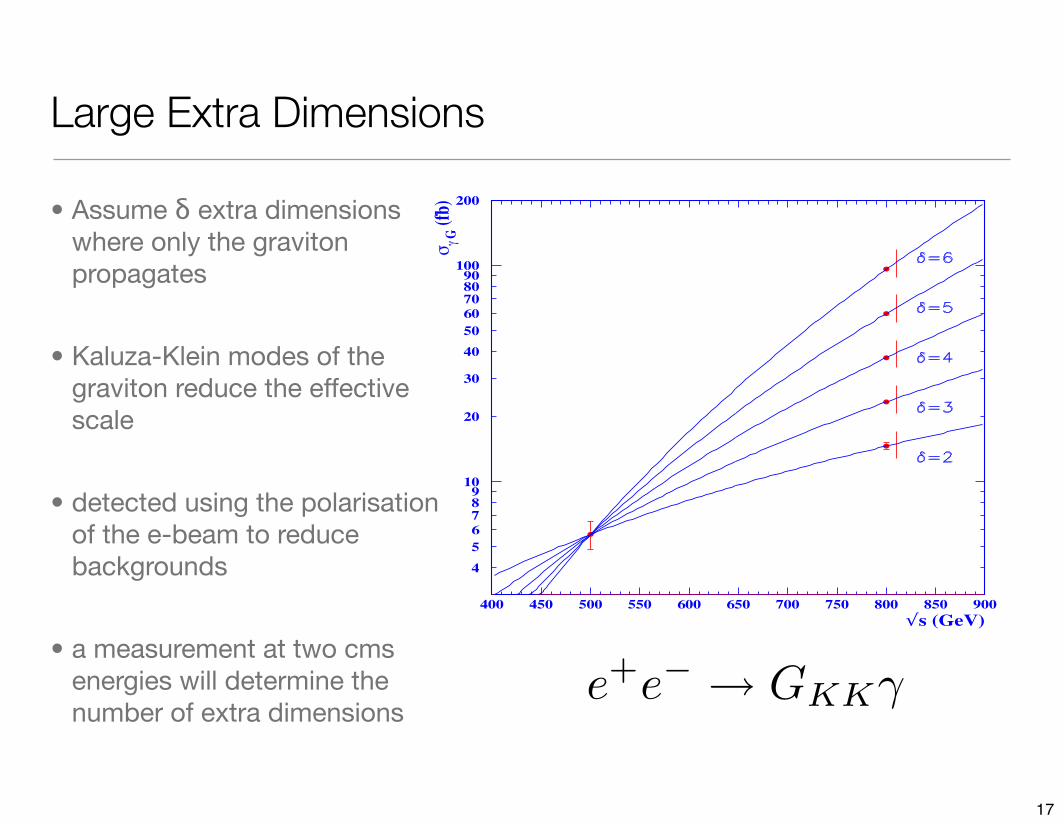
Once the missing energy signal is observed, the next step would be to confirm its gravita-tional nature and determine the number of extra dimensions. The ILC will play an essentialrole here. The number of extra dimensions can be determined from the energy dependenceof the production cross section. In the left–hand side of Fig. 6.2-1, it is shown that its mea-surement at two collider energies,

#s = 500 GeV and 800 GeV, can discriminate between

scenarios with di!erent numbers of extra dimensions. Additional information on the numberof extra dimensions can also be obtained from the missing mass distribution.

!s (GeV)

!"

G (

fb)

4

5

6

789

10

20

30

40

50

60

708090

100

200

400 450 500 550 600 650 700 750 800 850 900

FIGURE 6.2-1. Left: determination of the number of extra-dimensions at the ILC at two center of massenergies

#s = 500 and 800 GeV [213]. Right: the di!erential azimuthal asymmetry distribution for

e+e! " #+#! at 500 GeV ILC with 500 fb!1 data in the SM (histogram) and in the LED model with acut–o! of 1.5 TeV (data points); e± are assumed to be 80% and 60% polarized, respectively [214].

An alternative signal for the presence of extra dimensions is provided by KK–gravitonexchange in processes such as e+e! " f f̄ . The mass reach in this channel is similar to thatobtained in KK–graviton emission. Since many new physics models can generate deviations inthis reaction, it is important to discriminate the extra–dimensional model from other scenar-ios. s–channel KK–graviton exchange has the characteristic signature of spin–two particlein the angular distributions of the e+e! " f f̄ ,WW and HH production processes [215].Furthermore, if both electron and positron are transversely polarized, the azimuthal asym-metry distribution provides a powerful tool to identify the spin–two nature of the virtuallyexchanged particle [17, 214] as shown in the right–hand side of Fig. 6.2-1.

ILC Reference Design Report II-77

e+e! ! GKK!

Large Extra Dimensions

• Assume δ extra dimensions where only the graviton propagates

• Kaluza-Klein modes of the graviton reduce the effective scale

• detected using the polarisation of the e-beam to reduce backgrounds

• a measurement at two cms energies will determine the number of extra dimensions

17

International Linear Collider

• No longer circularwhere energy could repeatedly be transferred in the same structure

• Why still a ring?Damping rings are required to produce the low emittance beams

• complicated sourcesintensity issue

18

Radiation of a non-relativistic moving Charge

Ps =e2

6!"0m20c3

!

d#p

dt

"2

dPs

d!=

e2

16!2"0m20c3

!

d#p

dt

"2

sin2"

Power:

Hertz' Dipole:

Lamor

19

Radiation of a relativistic Charge

dt ! d! =1

"dt ! =

E

m0c2=

1!

1 ! "2where

!

dPµ

d!

"2

!

!

d"p

d!

"2

"

1

c2

!

dE

d!

"2

Ps =e2c

6!"0

1

(m0c2)2

!

"

d#p

d$

#2

!

1

c2

"

dE

d$

#2$

Replace:

Details J.D.Jackson

20

Radiation in Direction of Particle Motion

EdE

d!= c2p

dp

d!

Can be neglected w.r.t. accelerating gradient, only 10-13 of typical gradients.

Ps =e2c

6!"0(m0c2)2

!

dp

#d$

"2

Ps =e2c

6!"0(m0c2)2

!

dE

dx

"2dp

dt=

dE

dxWith

21

Transverse Acceleration

with

EdE

dt= 0

Ps =e2c

6!"0

1

(m0c2)2

E4

R2

dp

dt= p! = p

v

R

Ps =e2c

6!"0

1

(m0c2)2

!

dp

d#

"2

Ps =e2c!2

6"#0

1

(m0c2)2

!

dp

dt

"2

relativistic22

Energy loss per turn

!E =

!Psdt = Pstb = Ps

2!R

c

!E =e2

3!0(m0c2)4

E4

R

!E [keV] = 88.5E4

!

GeV4"

R [m]

23

Synchrotron Radiation – Angular dependence

P !

µ =

!

"

"

#

pt

px

py

pz

$

%

%

&

=

!

"

"

#

E!

s/c0

p!00

$

%

%

&

tan! =py

pz

=p!0

!"p!0

!

1

"

Single photon in y-direction

Pµ =

!

"

"

#

! 0 0 "!0 1 0 0

0 0 1 0

"! 0 0 !

$

%

%

&

!

"

"

#

E!

s/c0

p!00

$

%

%

&

=

!

"

"

#

!E!

s/c0

p!0!"E!

s/c

$

%

%

&

24

Radiation Pattern

Radiation Pattern Radiation Pattern

electron

accelerating force

radius

electron orbit

electron orbit

electron

accelerating force

radius

25

Time Structure

!t =2R"

c!!

2R sin "

c

=2R

c

!

"

!! " +

"3

3!!

"5

5!+ · · ·

"

"

2R

c

!

1

!"!

1

"+

1

6"3

"

"

4R

3c"3

!typ =2"

!t=

3"c#3

2R

Broad Frequency spectrum

observer

electron track

26

Spectral Density

! =

"

"c

! 1

0

Ss(!)d! =1

2

Definition of critical energy

E=5 GeV, R=12.2 m

X-rays and higher

critical energy

27

Examples of Energy Loss for Accelerators

Accelerator L [m] E [GeV] R [m] ΔE[MeV]

Doris 288 5.0 12.2 4.5

PETRA 2304 23.5 195 138

LEP I 27000 70 3000 708

LEP II 100 3000

28

Energy Loss per turn

0

100

200

300

400

500

600

700

800

0 50 100 150 200 250 300 350 400 450

Beam Energy [GeV]

∆E [

GeV

]

Extending LEP?

for R=3 km

29

Cost Scaling

•Linear cost: tunnel, magnets, infrastructure€lin ~ ρ

•RF cost€RF ~ E4 / ρ

•Optimum at€lin = €RF

Thus optimised cost (€lin + €RF ) scales as E2.

30

Solution: Linear Collider

• long linac constructed of many RF accelerating structures

• typical gradients 25 – 100 MV/m; ILC nominal gradient 31.5 MV/m

• cost scales as E

e+ e-

5-10 km

31

Solution: Linear Collider

• long linac constructed of many RF accelerating structures

• typical gradients 25 – 100 MV/m; ILC nominal gradient 31.5 MV/m

• cost scales as E

bang!e+ e-

5-10 km

31

Emittance in Linear Collider

• similarlyε = ε / γ

• angular divergence is reduced relativistically

l=l0*γ

boost

θ0 θ=θ0/γ

32

Luminosity

Collider luminosity is approximately given by

where:

L =

nbN2frep

AHD

L =nbN

2frep

4!"x"yHD

nb = bunches/train

N = particles per bunch

frep = repetition frequency

A = beam cross section at IP

HD = beam ! beam enhancement factor

for Gaussian beams

33

Luminosity: RF Power

With centre of mass energy

for Gaussian beam

L =(EcmnbNfrep)N

4!"x"yEcm

HD

L =!RFPRFN

4"#x#yEcm

HD

nbNfrepEcm = Pbeams

= !RFPRF

34

Luminosity: RF Power

Power Estimate

Need to include efficienciesRF⇒beam: range 20-60%

Wall plug ⇒ RF: range 28-40%

AC power >100 MW just to accelerate beams and achieve luminosity.

L =!RFPRFN

4"#x#yEcm

HD

Ecm = 500 GeVN = 1010

nb = 100frep = 100 (5) Hz

!

"

"

#

"

"

$

Pbeams = 8MW

Linac Technology!

35

Storage Ring vs LC

Repetition rateLEP: 44 kHzLC: few to 100 Hz

Compensate by beam cross section at IP

L =!RFPRFN

4"#x#yEcm

HD

Factor 400 lost!

LEP : !x!y ! 130 " 6µm2

LC : !x!y ! (200 # 500) " (3 # 5)nm2

Needed to obtain L = a few 1034

cm!2

s!1

Factor 106 gained!

36

Intense Beams at IP

L =1

4!("RFPRF)

!

N

#x#y

HD

"

Choice of linac technology- efficiency- available power

Beam-Beam effects- beamstrahlung- disruption

Strong focusing- optical aberrations- stability issues and tolerances

37

Luminosity Issue. Beam-beam Interaction

E y (M

V/c

m)

y/σy

• strong mutual focusing of beams (pinch) gives rise to luminosity enhancement HD

• As e± pass through intense field of opposing beam, they radiate hard photons [beamstrahlung] and loose energy

• Interaction of beamstrahlung photons with intense field causes copious e+e- pair production [background]

38

Beam Beam Interaction at IP

Beam beam characterized by Disruption parameter:

Dx,y =2reN!z

"!x,y(!x + !y)!

!z

fbeam

Enhancement factor (typically HD~2)

HDx,y= 1 + D1/4

x,y

!

D3x,y

1 + D3x,y

"#

$ln(%

Dx,y + 1) + 2 ln

&0.8!x,y

"z

'

( )* +

,

-

Hour glass effect

For storage rings fbeam~σz and Dx,y~1.In a LC, Dy~10-20 and hence fbeam<σz

39

Hour Glass Effect

β = “depth of focus”reasonable lower limit forβ is bunch length σz

40

RMS relative energy loss

Would like to make σx σy small to maximise luminosity.

BUT keep (σx + σy) large to reduce δSB.

Trick: use “flat beams” with

Now we set σx to fix δSB, and make σy as small as possible to achieve high luminosity.

For most LC designs, δSB ~ 3-10%

Beamstrahlung

!BS ! 0.86er3

e

2m0c2

!

Ecm

"z

"

N2

("x + "y)2

!BS !

!

Ecm

"z

"

N2

"2x

!x ! !y

41

Returning to our L scaling law, and ignoring HD

From flat-beam beamstrahlung

hence

Beamstrahlung

N

!x

!

!

!z"BS

ECM

L !!RFPRF

E3/2cm

""BS#z

#y

L !!RFPRF

ECM

!

N

"x

"

1

"y

42

So far:

L !!RFPRF

E3/2cm

""BS#z

#y

For high luminosity we need:

• high RF-beam conversion efficiency

• high RF power

• small vertical beam size

• large bunch length (to be reconsidered)

• and could allow for larger beamstrahlung if willing to live with consequences

43

Small vertical beam size

L !!RFPRF

E3/2cm

""BS#z

#y

!y =

!

"y#n,y

$

with εn,y normalised vertical emittance and βy the vertical β-function at the IP.

L !!RFPRF

E3/2cm

!

"BS#

$n,y

"

%z

&y!

!RFPRF

Ecm

!

"BS

$n,y

"

%z

&y

44

Optimised Scaling Law

L !!RFPRF

Ecm

!

"BS

#n,y

HD for $z " %y

• high RF-beam conversion efficiency

• high RF power

• small normalised vertical emittance

• strong focussing at IP (small βy and hence small σz!)

• and could allow for larger beamstrahlung if willing to live with consequences

45

Luminosity as a function of βy

46

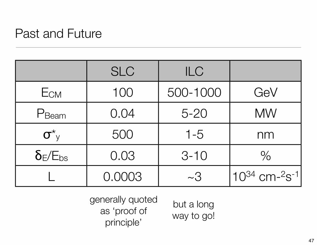
generally quoted as ‘proof of principle’

but a long way to go!

Past and Future

SLC ILC

ECM 100 500-1000 GeV

PBeam 0.04 5-20 MW

σ*y 500 1-5 nm

δE/Ebs 0.03 3-10 %

L 0.0003 ~3 1034 cm-2s-1

47

Components of the ILC

48

www.linearcollider.org

49